pset3 Solutions 2012 - Massachusetts Institute of...

E3-1 Estimate how many of the combined pools on the MIT campus of water are contained in a big fluffy cloud on a summer’s day. Report your answer in units of total MIT pool volumes.

To solve this problem, we need a solution in the units of (total water volume contained in a cloud) per (total volume ofMIT pools).

According to Scientific American (http://www.scientificamerican.com/article.cfm?id=why-do-clouds-float-when),there is about 1.0 gram of water per cubic meter in a cloud. This value is the water-density of a cloud, water per cubicmeter.

Accrding to an article published in the Journal of Climate and Applied Meteorology by B.A. Wielicki and R.M.Welch, “Cumulus Cloud Properties Derived Using Landsat Satelite Data” < http://journals.ametsoc.org/-doi/pdf/10.1175/1520-0450(1986)025%3C0261%3ACCPDUL%3E2.0.CO%3B2 >,a typical cumulus cloud is roughly several km tall (take 5 km), and a a few km on each side (let’s take 2 km for a bigone). Therefore, the total volume of a typical large cumulus cloud is 2 km × 2 km × 5 km. The mass of water containedin the cloud is this volume times the density, which is 10-3 kgëm3.

massh2o = H2000L2 H5000L 10-3

H* water mass in kg = volume of cloud in m3 times cloud water density, kgëm3 *L

20 000 000

The density of fresh (cloud) water is 1.0 gëcm3, so the volume of water in a cloud is:

volh2o = massh2o ë 1000 H* water volume,

m3 = water mass in kg divided by water density in kgëm3 *L

20 000

This is the (total water volume contained in a cloud). This is the numerator of the desired solution.

There are 3 pools at MIT: the alumni gym pool, the main, olympic-size Z-center pool, and a small Z-center pool. Fromexperience looking at these pools, the Alumni pool is about 40 m × 15 m × 2 m deep, the olympic pool is 50 m × 25 m× about 3 m deep (it has variable depth, so this includes the very deep diving end of the pool), and the small Z-centerpool is roughly 20 m × 10 m × 2 m. The total MIT pool volume is:volpools = 40 µ 15 µ 2 H* alumni *L + 50 µ 25 µ 3 H* Z-center olympic pool *L + 20 µ 10 µ 2

H* small Z-center *L H* all values in meters, so volpools has units of m3 *L

5350

This is (total volume of MIT pools), which is the denomenator of the desired result. Combining the numerator anddenominator givesNüvolh2o ê volpools H* cloud water volume ê MIT pool volume *L

3.73832

There are about 4 MIT pool-volumes of water contained in a large cumulus cloud.

I3-1 Solve the following system of two equations for x and y.

I3-1 Solve the following system of two equations for x and y.

i. Solve for x & yYour solution should be handworked; however, the solutions with be provided with Mathematica. The function“Solve” can be used to find x & y in terms of t and z.solution = Solve@812 ã 3 x + 4 y - 5 z + 10 t, 0 ã -x + 2 y - 5 z + 20 t<, 8x, y<D

::x Ø12

5+ 6 t - z, y Ø

6

5- 7 t + 2 z>>

A trick to actually define the equation for x as given above by “solution” uses ReplaceAll (/.) and Part ([[ ]]).“xequation” and “yequation” are the expressions for x and y.xequation = x ê. solution@@1DD

12

5+ 6 t - z

yequation = y ê. solution@@1DD

6

5- 7 t + 2 z

ii. Find the restrictions on t & zFollowing the hint from pset #2, use Reduce to find the restrictions on t ans z.bounds = Reduce@xequation > 0 && yequation > 0, 8t, z<D

t > -6

5&&

1

10H-6 + 35 tL < z <

1

5H12 + 30 tL

iii. Plot the region where x & y > 0 on the t-z planeThe restriction on t is simple, it just has to be larger than -6/5, so plot z = 1

10H-6 + 35 tLand z = 1

5H12 + 30 tL for

t > -6/5, and the wedge between these two lines is the desired region, where x & y are greater than zero.

2 pset3_Solutions_2012.nb

RegionPlot@bounds, 8t, -2, 10<, 8z, -10, 60<, ColorFunction Ø Blue,AxesLabel Ø 8Style@"t", FontSize Ø 28D, Style@"z", FontSize Ø 28D<, PlotLabel Ø Pane@

Style@"Region where x & y are positive on the z vs. t plane", FontSize Ø 24D, 300DD

I3-2 For the van der Waals equation of state, introduce non-dimensional variables (P, W, and Q) in terms of the critical pressure, volume, and temperature.

i. Units of P, W, and Q?P, W, and Q are dimensionless.

ii. For what values of P, W, and Q does the critical point appear?When P, W, and Q are equal to 1, the critical point appears.

iii. Plot 5 isotherms on the P-W plane.Recycling our result from pset #2, we found that

pset3_Solutions_2012.nb 3

Pcrit = a ë I27 b2M;Vcrit = 3 b;Tcrit = 8 a ê H27 b RL;

With the substitutions given in the problem statement, the Van Der Waals gas equation becomes:vdwLhs = FullSimplify@

HHP + a ê V^2L HV - bL L ê. 8T Ø Tcrit Q, V Ø Vcrit W, P Ø Pcrit P<D H* left hand side *L

a H-1 + 3 WL I3 + P W2M

27 b W2

vdwRhs = FullSimplify@HR T L ê. 8T Ø Tcrit Q, V Ø Vcrit W, P Ø Pcrit P<

D H* right hand side *L

8 a Q

27 b

set Lhs = Rhs, and solve for P:Pvdw = Simplify@P ê. HSolve@vdwLhs ã vdwRhs, PD êê FlattenLD

3 - 9 W + 8 Q W2

W2 H-1 + 3 WL

This is the non-dimensionalized van der Waals equation.

Now that we have our non-dimensional expression for P, plot it, here with cold colors grading into hot colors as Qincreases:


Show@Plot@Evaluate@Sequence@Table@Pvdw, 8Q, 80.8, 0.9, 1, 1.1, 1.2<<DDD,8W, 0.4, 1.2<, PlotStyle Ø 8Purple, Blue, Green, Orange, Red<,PlotLabel Ø Style@"Isotherms of P", FontSize Ø 28D,AxesLabel Ø 8Style@"W", FontSize Ø 20D, Style@"P", FontSize Ø 20D<D,

Graphics@8Red, Text@Style@"Q = 1.2", FontSize Ø 16D, 81.1, 6.5<D,Orange, Text@Style@"Q = 1.1", FontSize Ø 16D, 81.1, 6.<D,Green, Text@Style@"Q = 1", FontSize Ø 16D, 81.1, 5.5<D,Blue, Text@Style@"Q = 0.9", FontSize Ø 16D, 81.1, 5<D,Purple, Text@Style@"Q = 0.8", FontSize Ø 16D, 81.1, 4.5<D<DD

Q = 1.2Q = 1.1Q = 1Q = 0.9Q = 0.8

0.6 0.8 1.0 1.2 W

1

2

3

4

5

6

PIsotherms of P

iv. Plot the surface that represents the van der Waals equation.Plot3D@Pvdw, 8Q, 0.2, 1.2<, 8W, 0.35, 1.1<, AxesLabel Ø

8Style@"Q", FontSize Ø 20D, Style@"W", FontSize Ø 20D, Style@"P", FontSize Ø 20D<,PlotLabel Ø Style@"PHQ, WL", FontSize Ø 28DD

v. Find the values of the van der Waals constants a and b for water vapor. Draw the isotherms near the critical temperature for water vapor.


v. Find the values of the van der Waals constants a and b for water vapor. Draw the isotherms near the critical temperature for water vapor.

For water, a = 5.536 L2 atmëmol2 = 0.560935 m4 N ëmol2 b = 0.03049 L/mol = 0.00003049 m3 ëmol, fromWikipediaaWater = 0.560935;bWater = 0.00003049;R = 8.31446; H* Jêmol K *L

tcritWater =8 aWater

27 bWater R655.613

Tcrit for water is ~655 K, so plot isotherms near this value (I chose 550, 600, 650, & 700):

ShowBPlotBEvaluateBSequenceBTableB-aWater

V2+

R T

-bWater + V, 8T, 8550, 600, 650, 700<<FFF,

8V, bWater, 20 bWater<, PlotRange Ø 980, 20 bWater<, 107 8-0.1, 4<=,PlotStyle Ø 8Blue, Green, Orange, Red<,PlotLabel Ø Style@"Isotherms of P for Water", FontSize Ø 28D, AxesLabel Ø

8Style@"Volume HLL", FontSize Ø 20D, Style@"Pressure HPaL", FontSize Ø 20D<F,

GraphicsA9Blue, TextAStyle@"T = 550 K", FontSize Ø 18D, 90.0002, 1 µ 107=E,

Green, TextAStyle@"T = 600 K", FontSize Ø 18D, 90.00015, 1.45 µ 107=E,

Orange, TextAStyle@"T = 650 K", FontSize Ø 18D, 90.00012, 1.85 µ 107=E,

Red, TextAStyle@"T = 700 K", FontSize Ø 18D, 90.0002, 2.5 µ 107=E=EF

T = 550 K

T = 600 KT = 650 K

T = 700 K

0.0001 0.0002 0.0003 0.0004 0.0005 0.0006Volume HLL0

1µ 107

2µ 107

3µ 107

4µ 107Pressure HPaL

Isotherms of P for Water

vi. What are the units of b? Think physically about what the sign of b means.


vi. What are the units of b? Think physically about what the sign of b means.

b = -V dP/dVV has units of m3 ëmol, dP/dV has units of Pressure/molar volume, N molëm5, so b must have units N ëm2 = Pa.

If P goes down as V increases (like the real world), then b is positive. If it were not positive, a baloon would expandunstablely, or shrink to a point.

vii. Find a non-dimensional representation of bLet B = b / Pcrit.

dPdV

= dHPêPcritLdHVêVcritL

= dPdW

VcritPcrit

B = -V dPdV

ëPcrit = -HW VcritL dPdW

PcritVcrit

H1 êPcritL = -W dPdW

B = -W D@Pvdw, WD

-W-9 + 16 Q W

W2 H-1 + 3 WL-3 I3 - 9 W + 8 Q W2M

W2 H-1 + 3 WL2-2 I3 - 9 W + 8 Q W2M

W3 H-1 + 3 WL

“B” is the non-dimensionalized equation for b.


viii. Plot the values where b is negative on the Q-W planePlot3D@B, 8W, 0.2, 1.8<, 8Q, 0.1, 1.2<, PlotRange Ø 8All, All, 80, 60<<,ClippingStyle Ø 8LighterüRed, LighterüCyan<, AxesLabel Ø 8Style@"W", FontSize Ø 20D,

Style@"Q", FontSize Ø 20D, Style@"B Hnon-dimensional bL", FontSize Ø 20D<,PlotLabel Ø Style@"The region where BHQ, WL is positive" , FontSize Ø 20D,Epilog Ø Inset@Framed@Style@"surface & blue = positive » red = negative", 16DD,

8Right, Bottom<, 8Right, Bottom<DD

Another way to visualize the same thing:


ShowBContourPlotB3 - 9 W + 8 Q W2

W2 H-1 + 3 WL, 8W, 0.3, 1.2<,

8Q, 0.1, 1.2<, ColorFunction Ø "BlueGreenYellow",AxesLabel Ø 8Style@"W", FontSize Ø 20D, Style@"Q", FontSize Ø 20D<,

PlotLabel Ø Style@"BHQ, WL" , FontSize Ø 20D F,

RegionPlot@B < 0, 8W, 0.3, 1.2<, 8Q, 0.1, 1.2<, PlotStyle Ø PinkDF

The blue-green-yellow contours show where B is positive (real world), the pink region is where B is negative (non-physical)

ix. Repeat the above for water vapor.Plot b = - V dP/dV for water:b = B Pcrit = B aWater/(27 bWater2)

bWater = -V DB-aWater

V2+

R T

-bWater + V, VF

- -8.31446 T

H-0.00003049 + VL2+1.12187

V3V


Plot3DAbWater, 8V, bWater + 0.0001, 100 bWater<, 8T, 10, 1000<,

PlotRange Ø 9All, All, 90, 107==, ClippingStyle Ø 8LighterüRed, LighterüCyan<,AxesLabel Ø 8Style@"V HLL", FontSize Ø 20D, Style@"T HKL", FontSize Ø 20D,

Style@"bH2 O HPaL", FontSize Ø 20D<, PlotLabel Ø Style@"bwater", FontSize Ø 28D,Epilog Ø Inset@Framed@Style@"surface & blue = positive » red = negative", 16DD,

8Right, Bottom<, 8Right, Bottom<DE

x. What are the units of thermal expansion, a?a = 1

V dVdT

The units are the same as 1/T, because the V and dV cancel out. Therefore, the units of a are 1/K.

In the real world, if you heat up a gas at fixed pressure, it expands. Therefore, a is positive. If it were not, then if youheated up the gas in a baloon, it would shrink.

xi. Find a non-dimensional representation of a.To non-dimensionalize, multiply by a characteristic temperature to cancel out the units of a:A = a Tcrit = I 1

WVcritM dWdQ

IVcritTcrit

M Tcrit = H1 êWL dWdQ

To express A, find W as a function of P and Q by rearranging the van er Waals equation. It is not a short equation, sothe output is suppressed for both W and A.Wvdw = Simplify@W ê. HSolve@vdwLhs ã vdwRhs, WD êê FlattenLD;

A = H1 ê WvdwL D@Wvdw, QD;


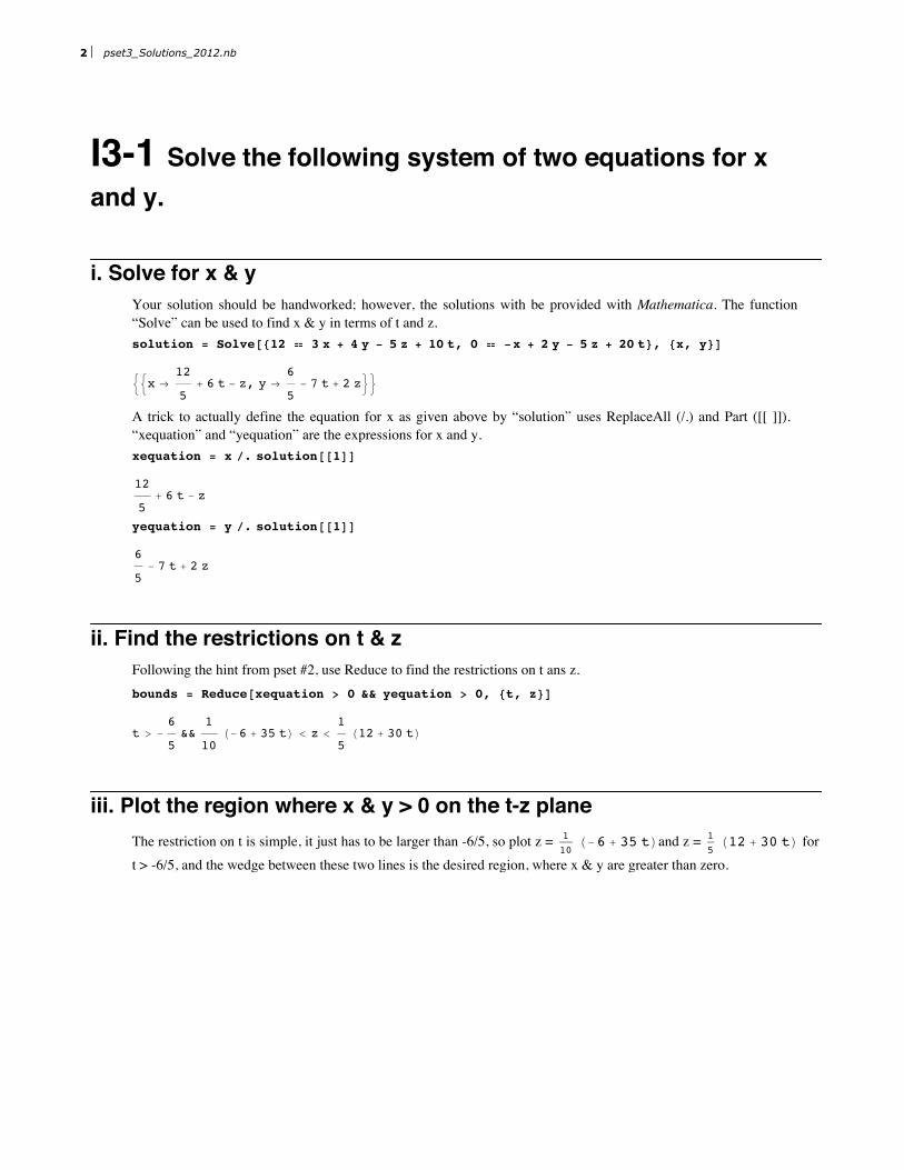
xii. Plot where a is negative on the Q-P plane.Plot3D@A, 8P, 0.2, 1.8<, 8Q, 0.1, 1.2<, PlotRange Ø 8All, All, 8-1, 0<<,ClippingStyle Ø 8Red, LighterüCyan<, AxesLabel Ø 8Style@"P", FontSize Ø 20D,

Style@"Q", FontSize Ø 20D, Style@"A Hnon-dimensional aL", FontSize Ø 20D<,PlotLabel Ø Style@"AHP, WL", FontSize Ø 28D,Epilog Ø Inset@Framed@Style@"blue = positive » red & hole = negative", 16DD,

8Right, Bottom<, 8Right, Bottom<DD

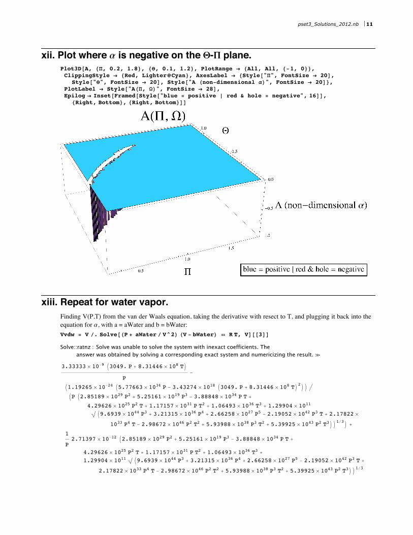
xiii. Repeat for water vapor.Finding V(P,T) from the van der Waals equation, taking the derivative with resect to T, and plugging it back into theequation for a, with a = aWater and b = bWater:Vvdw = V ê. Solve@HP + aWater ê V^2L HV - bWaterL ã R T, VD@@3DD

Solve::ratnz : Solve was unable to solve the system with inexact coefficients. Theanswer was obtained by solving a corresponding exact system and numericizing the result. à

3.33333 µ 10-9 I3049. P + 8.31446 µ 108 TM

P-

I1.19265 µ 10-24 I5.77663 µ 1034 P - 3.43274 µ 1018 I3049. P + 8.31446 µ 108 TM2MM ë

IP I2.85189 µ 1029 P2 + 5.25161 µ 1019 P3 - 3.88848 µ 1034 P T +

4.29626 µ 1025 P2 T + 1.17157 µ 1031 P T2 + 1.06493 µ 1036 T3 + 1.29904 µ 1011,I9.6939 µ 1044 P3 + 3.21315 µ 1036 P4 + 2.66258 µ 1027 P5 - 2.19052 µ 1042 P3 T + 2.17822 µ

1033 P4 T - 2.98672 µ 1046 P2 T2 + 5.93988 µ 1038 P3 T2 + 5.39925 µ 1043 P2 T3MM1ê3M +

1

P2.71397 µ 10-12 I2.85189 µ 1029 P2 + 5.25161 µ 1019 P3 - 3.88848 µ 1034 P T +

4.29626 µ 1025 P2 T + 1.17157 µ 1031 P T2 + 1.06493 µ 1036 T3 +1.29904 µ 1011 ,I9.6939 µ 1044 P3 + 3.21315 µ 1036 P4 + 2.66258 µ 1027 P5 - 2.19052 µ 1042 P3 T +

2.17822 µ 1033 P4 T - 2.98672 µ 1046 P2 T2 + 5.93988 µ 1038 P3 T2 + 5.39925 µ 1043 P2 T3MM1ê3


aWater = H1 ê VvdwL D@Vvdw, TD;

Plot3DAaWater, 9P, 0, 108=, 8T, 10, 1000<, PlotRange Ø 8All, All, 80, 0.04<<,ClippingStyle Ø 8LighterüRed, LighterüCyan<, MaxRecursion Ø 5,AxesLabel Ø 8Style@"P HPaL", FontSize Ø 20D, Style@"T HKL", FontSize Ø 20D,

Style@"aH2 O H1êKL", FontSize Ø 20D<, PlotLabel Ø Style@"awater", FontSize Ø 32D,Epilog Ø Inset@Framed@Style@"blue & surface = positive » red & hole = negative", 16DD,

8Right, Bottom<, 8Right, Bottom<DE

The plot is not well resolved near the non-pysical region, where a is negative. The peaks and valleys are an artifiact ofhow Mathematica generates plots, not a feature of a.

I3-3 This problem is an example of how to interact with Mathematica and infer the nature of general solutions. Consider the systems of linear springs with differing spring constants Hki) and “zero-strain” lengths (Li).

i. For the system of two springs, construct a matrix that multiplies the unknowns Hx1, x2) and gives the right-hand-side vector at equilibrium. Solve this matrix equation to obtain the equilibrium positions x1 and x2 in terms of the applied force.

For 2 springs:F2is set to be some known applied force. What are the equilibrium positions of the middle node, x1, and the end nodex2, and what is the force on the first spring, F1?

There are 3 unknowns. Therefore, 3 equations are required to solve. These equations are:1. Hooke’s law for spring 1: F1 = -k1 dx12. Hooke’s law for spring 2: F2 = -k2 dx23. Force balance on the center node (this node is stationary at equilibrium, so the net force is zero): F1 = F2 => k1dx1 = k2 dx2

dx1 = x1 - L1 - x0dx2 = x2 - L2 - x1

In all, the 3 equations, with some algebraic rearrangement, are:

1: F1 + k1 x1 = k1 L1 + k1 x02: -k2 x2 + k2 x1 = F2 - k2 L23: (k1 + k2) x1 - k2 x2 = k1 L1 + k1 x0 - k2 L2

Writing them in a more suggestive form:

1: 1 F1 + k1 x1 + 0 x2 = k1 L1 + k1 x02: 0 F1 + k2 x1 + -k2 x2 = F2 - k2 L23: 0 F1 + (k1+k2) x1 + -k2 x2 = k1 L1 + k1 x0 - k2 L2

This now looks like the result of a matrix multiplication:

1 k1 000

k2k1 + k2

-k2-k2

F1x1x2

= k1 L1 + k1 x0

F2 - k2 L2k1 L1 + k1 x0 - k2 L2


For 2 springs:F2is set to be some known applied force. What are the equilibrium positions of the middle node, x1, and the end nodex2, and what is the force on the first spring, F1?

There are 3 unknowns. Therefore, 3 equations are required to solve. These equations are:1. Hooke’s law for spring 1: F1 = -k1 dx12. Hooke’s law for spring 2: F2 = -k2 dx23. Force balance on the center node (this node is stationary at equilibrium, so the net force is zero): F1 = F2 => k1dx1 = k2 dx2

dx1 = x1 - L1 - x0dx2 = x2 - L2 - x1

In all, the 3 equations, with some algebraic rearrangement, are:

1: F1 + k1 x1 = k1 L1 + k1 x02: -k2 x2 + k2 x1 = F2 - k2 L23: (k1 + k2) x1 - k2 x2 = k1 L1 + k1 x0 - k2 L2

Writing them in a more suggestive form:

1: 1 F1 + k1 x1 + 0 x2 = k1 L1 + k1 x02: 0 F1 + k2 x1 + -k2 x2 = F2 - k2 L23: 0 F1 + (k1+k2) x1 + -k2 x2 = k1 L1 + k1 x0 - k2 L2

This now looks like the result of a matrix multiplication:

1 k1 000

k2k1 + k2

-k2-k2

F1x1x2

= k1 L1 + k1 x0

F2 - k2 L2k1 L1 + k1 x0 - k2 L2

ü Solving for x1, x2, and F1 by solving the system of equationsClear@k, x, F, eqD

The first equation: F1= k1 dx1 eq@1D = F@1D ã -k@1D Hx@1D - x@0D - L@1DL

F@1D ã -k@1D H-L@1D - x@0D + x@1DL

The second equation: F2 = k2 dx2eq@2D = F@2D ã - k@2D Hx@2D - x@1D - L@2DL

F@2D ã -k@2D H-L@2D - x@1D + x@2DL

The third equation: F1 = F2:eq@3D = k@1D Hx@1D - x@0D - L@1DL ã k@2D Hx@2D - x@1D - L@2DL

k@1D H-L@1D - x@0D + x@1DL ã k@2D H-L@2D - x@1D + x@2DL

Solve these 3 equations together:systemResult = Solve@8eq@1D, eq@2D, eq@3D<, 8x@1D, x@2D, F@1D<D@@1DD

:x@1D Ø -F@2D - k@1D L@1D - k@1D x@0D

k@1D, x@2D Ø -

F@2D

k@1D-F@2D

k@2D+ L@1D + L@2D + x@0D, F@1D Ø F@2D>


x1sys = x@1D ê. systemResultx2sys = x@2D ê. systemResultF1sys = F@1D ê. systemResult

-F@2D - k@1D L@1D - k@1D x@0D

k@1D

-F@2D

k@1D-F@2D

k@2D+ L@1D + L@2D + x@0D

F@2D

This gives the positions of the nodes and F1 in terms of F2, x0, L1, L2, k1, and k2. Note that F1 = F2 falls out.

ü Solving for x1, x2, and F1 using direct input of matrix and b-vectormatrixA = 881, k@1D, 0<, 80, k@2D, -k@2D<, 80, k@1D + k@2D, -k@2D<<;MatrixForm@matrixAD

1 k@1D 00 k@2D -k@2D0 k@1D + k@2D -k@2D

unknownVector = 8F@1D, x@1D, x@2D<;MatrixForm@unknownVectorD

F@1Dx@1Dx@2D

vectorB = 8k@1D L@1D + k@1D x@0D, F@2D - k@2D L@2D, k@1D L@1D + k@1D x@0D - k@2D L@2D<;MatrixForm@vectorBD

k@1D L@1D + k@1D x@0DF@2D - k@2D L@2D

k@1D L@1D - k@2D L@2D + k@1D x@0D

Solve the linear system:linearResult = LinearSolve@matrixA, vectorBD

:F@2D, -F@2D

k@1D+ L@1D + x@0D,

1

k@1D k@2D

H-F@2D k@1D - F@2D k@2D + k@1D k@2D L@1D + k@1D k@2D L@2D + k@1D k@2D x@0DL>

Define the outputs:x1lin = linearResult@@2DDx2lin = linearResult@@3DDF1lin = linearResult@@1DD

-F@2D

k@1D+ L@1D + x@0D

1

k@1D k@2DH-F@2D k@1D - F@2D k@2D + k@1D k@2D L@1D + k@1D k@2D L@2D + k@1D k@2D x@0DL

F@2D

Are the results equivalent?


Simplify@x1sys ã x1linDSimplify@x2sys ã x2linDSimplify@F1sys ã F1linD

True

True

True

This shows that solving the matrix form is equivalent to solving the system of equations.

ü Solving for x1, x2, and F1 using Mathematica to generate the A matrix and b vectorThe same three equations are rearranged so that the left-hand side (LHS) is zerozeroEq@1D = -k@1D Hx@1D - L@1D - x@0DL - F@1DzeroEq@2D = k@1D Hx@1D - L@1D - x@0DL - k@2D Hx@2D - x@1D - L@2DLzeroEq@3D = -k@2D Hx@2D - x@1D - L@2DL - F@2D

-F@1D - k@1D H-L@1D - x@0D + x@1DL

k@1D H-L@1D - x@0D + x@1DL - k@2D H-L@2D - x@1D + x@2DL

-F@2D - k@2D H-L@2D - x@1D + x@2DL

The list of unknowns:vars = 8x@1D, x@2D, F@1D<

8x@1D, x@2D, F@1D<

This function, row[i], generates the coefficients of each variable for a given equation. These are the coefficients withconstruct the matrix A.row@i_D := Table@Coefficient@zeroEq@iD, vars@@jDDD, 8j, 1, 3<D

row@1Drow@2Drow@3D

8-k@1D, 0, -1<

8k@1D + k@2D, -k@2D, 0<

8k@2D, -k@2D, 0<

Compute the vector of constants, b, or RHS of the linear algebra equation, by finding the terms that do not depend onthe vars using “Thread” (note the minus sign, because these terms are shifted to the opposite side of the equals sign)rhs = Table@-zeroEq@iD ê. Thread@Rule@vars, 0DD, 8i, 1, 3<D

8k@1D H-L@1D - x@0DL, -k@2D L@2D - k@1D H-L@1D - x@0DL, F@2D - k@2D L@2D<

Compute the matrix, A, using the function defined earlier, “row”matrix = Table@row@iD, 8i, 1, 3<D

88-k@1D, 0, -1<, 8k@1D + k@2D, -k@2D, 0<, 8k@2D, -k@2D, 0<<

Finally, invert A and matrix-multiply it into b to arrive at the solutionaltResult = Simplify@[email protected]

:-F@2D

k@1D+ L@1D + x@0D, -

F@2D Hk@1D + k@2DL

k@1D k@2D+ L@1D + L@2D + x@0D, F@2D>

x1alt = altResult@@1DD;x2alt = altResult@@2DD;F1alt = altResult@@3DD;


Demonstration that this alternative solution is identical to the previous two:Simplify@x1sys ã x1altDSimplify@x2sys ã x2altDSimplify@F1sys ã F1altD

True

True

True

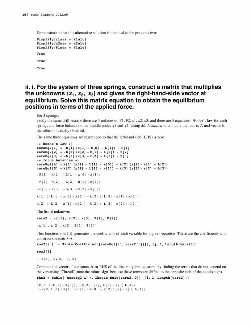
ii. i. For the system of three springs, construct a matrix that multiplies the unknowns Hx1, x2, x3) and gives the right-hand-side vector at equilibrium. Solve this matrix equation to obtain the equilibrium positions in terms of the applied force.

For 3 springs:exctly the same drill, except there are 5 unknowns: F1, F2, x1, x2, x3; and there are 5 equations: Hooke’s law for eachspring, and force balance on the middle nodes x1 and x2. Using Mathematica to compute the matrix A and vector b,the solution is easily obtained.The same three equations are rearranged so that the left-hand side (LHS) is zeroH* hooke's law *LzeroEq2@1D = -k@1D Hx@1D - x@0D - L@1DL - F@1DzeroEq2@2D = -k@2D Hx@2D - x@1D - L@2DL - F@2DzeroEq2@3D = -k@3D Hx@3D - x@2D - L@3DL - F@3DH* force balances *LzeroEq2@4D = k@1D Hx@1D - L@1D - x@0DL - k@2D Hx@2D - x@1D - L@2DLzeroEq2@5D = k@2D Hx@2D - L@2D - x@1DL - k@3D Hx@3D - x@2D - L@3DL

-F@1D - k@1D H-L@1D - x@0D + x@1DL

-F@2D - k@2D H-L@2D - x@1D + x@2DL

-F@3D - k@3D H-L@3D - x@2D + x@3DL



The list of unknowns:vars2 = 8x@1D, x@2D, x@3D, F@1D, F@2D<

8x@1D, x@2D, x@3D, F@1D, F@2D<

This function, row2[i], generates the coefficients of each variable for a given equation. These are the coefficients withconstruct the matrix A.row2@i_D := Table@Coefficient@zeroEq2@iD, vars2@@jDDD, 8j, 1, Length@vars2D<D

row2@1D

8-k@1D, 0, 0, -1, 0<

Compute the vector of constants, b, or RHS of the linear algebra equation, by finding the terms that do not depend onthe vars using “Thread” (note the minus sign, because these terms are shifted to the opposite side of the equals sign)rhs2 = Table@-zeroEq2@iD ê. Thread@Rule@vars2, 0DD, 8i, 1, Length@vars2D<D

8k@1D H-L@1D - x@0DL, -k@2D L@2D, F@3D - k@3D L@3D,-k@2D L@2D - k@1D H-L@1D - x@0DL, k@2D L@2D - k@3D L@3D<


Compute the matrix, A, using the function defined earlier, “row”matrix2 = Table@

Table@Coefficient@zeroEq2@iD, vars2@@jDDD, 8j, 1, Length@vars2D<D, 8i, 1, Length@vars2D<D

88-k@1D, 0, 0, -1, 0<, 8k@2D, -k@2D, 0, 0, -1<, 80, k@3D, -k@3D, 0, 0<,8k@1D + k@2D, -k@2D, 0, 0, 0<, 8-k@2D, k@2D + k@3D, -k@3D, 0, 0<<

Finally, invert A and matrix-multiply it into b to arrive at the solutionresult2 = Simplify@[email protected]

:-F@3D

k@1D+ L@1D + x@0D, -

F@3D Hk@1D + k@2DL

k@1D k@2D+ L@1D + L@2D + x@0D,

F@3D -1

k@1D-

1

k@2D-

1

k@3D+ L@1D + L@2D + L@3D + x@0D, F@3D, F@3D>

x1part2 = result2@@1DD;x2part2 = result2@@2DD;x3part2 = result2@@3DD;F1part2 = result2@@4DD;F2part2 = result2@@5DD;

An intersting experiment: inverstigate whether the solution with 2 springs is the same as the solution with 3 springs:Simplify@x1part2 ã x1linDSimplify@x2part2 ã x2linDSimplify@F1part2 ã F1linD

F@2D - F@3D

k@1Dã 0

HF@2D - F@3DL Hk@1D + k@2DL

k@1D k@2Dã 0

F@2D ã F@3D

We see from the solution to part 2, F1 = F2 = F3. Assume that the applied force is the same in parts 1 and 2, so F2 =F3. Comparing the solutions for x1 from part 1 and part 2 of this problem yields “F2-F3 = 0.” But, F2 = F3, so the x1position is identical whether there are 2 or 3 springs. For x2, we again see F2-F3, which is zero, so the position is thesame in parts 1 and 2. Finally, we see the forces are all the same as well. In short, if the applied force is the same, eachspring acts independantly - it does not matter how many springs are in the chain.

iii. By inspecting the solutions above, write a general function which takes a list of ki and Li and returns the positions xi .

By looking at part 2, we see that Hooke’s law always takes the form:0 = ki (xi - x(i-1) - Li) - Fiand if there are n springs, then we have n equations.

The force balances always take the form:0 = ki ( xi - x(i-1) - Li) - k(i+1) (x(i+1) - xi - L(i+1) )and if we have n springs, we generate n-1 equations.

So, we have in total 2n-1 equations, and 2n-1 variables: x1, x2, ... xn, F1, F2, ... F(n-1).

The function “springSolver” simply does everything that was shown in part 2, and puts each step inside a Module (sothat variable names are local). It takes a list of k’s and L’s, and outputs x’s and F’s.


springSolver@kis_, lis_D := Module@8n, listOfHookesEqns, listOfBalanceEqns, eqns, vars, matrixA, vectorb, solution<,

H* determine how make springs there are *Ln = Length@kisD;

H* find the equations in the form 0 = LHS, and generate a list of LHS's *LlistOfHookesEqns = Table@-kis@@iDD Hx@iD - x@i - 1D - lis@@iDDL - F@iD, 8i, n<D;listOfBalanceEqns = Table@kis@@iDD Hx@iD - x@i - 1D - lis@@iDDL -

kis@@i + 1DD Hx@i + 1D - x@iD - lis@@i + 1DDL, 8i, n - 1<D;H* join the two lists to get all 2n-1 equations together *Leqns = Join@listOfHookesEqns, listOfBalanceEqnsD;

H* write the list of variables *Lvars = Join@Table@x@iD, 8i, n<D, Table@F@iD, 8i, n - 1<DD;

H* generate the matrix *LmatrixA =Table@Table@Coefficient@eqns@@iDD, vars@@jDDD, 8j, Length@varsD<D, 8i, Length@eqnsD<D;

H* generate the RHS, b *Lvectorb = Table@-eqns@@iDD ê. Thread@Rule@vars, 0DD, 8i, Length@varsD<D;

H* compute the solution *Lsolution = LinearSolve@matrixA, vectorbD;

H* output the list of unknowns in in the followingformat: 88x@1D, value<, 8x@2D, value<, ... 8F@n-1D, value<< *L

Transpose@8vars, solution<DD

Test springSolver by comparing its solution for 2 springs to the solution to part 1:soln = springSolver@8k@1D, k@2D<, 8L@1D, L@2D<Dx1sol = soln@@1, 2DD;x2sol = soln@@2, 2DD;F1sol = soln@@3, 2DD;

::x@1D, -F@2D

k@1D+ L@1D + x@0D>,

:x@2D, -F@2D

k@1D+

-F@2D + k@2D L@1D + k@2D L@2D + k@2D x@0D

k@2D>, 8F@1D, F@2D<>

Simplify@x1sol ã x1linDSimplify@x2sol ã x2linDSimplify@F1sol ã F1linD

True

True

True

The comparisons all yielded true, so the solutions obtained in part 1 are identical to those produced by the functionspringSolver.


pset3 Solutions 2012 - Massachusetts Institute of...

Documents

Transcript of pset3 Solutions 2012 - Massachusetts Institute of...