Porosity, pore-size distribution and poresurface area of the Apache Leap tuff near

Superior, Arizona using mercury porosimetry

Item Type Thesis-Reproduction (electronic); text

Authors Vogt, Gerald Thomas,1960-

Publisher The University of Arizona.

Rights Copyright © is held by the author. Digital access to this materialis made possible by the University Libraries, University of Arizona.Further transmission, reproduction or presentation (such aspublic display or performance) of protected items is prohibitedexcept with permission of the author.

Download date 05/05/2018 18:13:21

Link to Item http://hdl.handle.net/10150/191980

POROSITY, PORE-SIZE DISTRIBUTION AND PORE SURFACE AREA

OF THE APACHE LEAP TUFF NEAR SUPERIOR, ARIZONA

USING MERCURY POROSIMETRY

by

Gerald Thomas Vogt

A Thesis Submitted to the Faculty of the

DEPARTMENT OF HYDROLOGY AND WATER RESOURCES

In Partial Fulfillment of the RequirementsFor the Degree of

MASTER OF SCIENCEWITH A MAJOR IN HYDROLOGY

Ir the Graduate College

THE UNIVERSITY OF ARIZONA

1988

STATEMENT BY AUTHOR

This thesis has been submitted in partial fulfillment ofrequirements for an advanced degree at The University of Arizona and isdeposited in the University Library to be made available to borrowersunder rules of the Library.

Brief quotations from this thesis are allowable without specialpermission, provided that accurate acknowledgment of source is made.Requests for permission for extended quotation from or reproduction ofthis manuscript in whole or in part may be granted by the head of themajor department or the Dean of the Graduate College when in his or herjudgment the proposed use of the material is in the interests ofscholarship. In all other instances, however, permission must beobtained from the author.

SIGNED:

APPROVAL BY THESIS DIRECTOR

This thesis has been approved on the date shown below:

D. D. EVANSProfessor of Hydrology and Water Resources

ate-

With love, I dedicate

this thesis to

my parents

111

ACKNOWLEDGMENTS

This research was performed at the University of Arizona under

the guidance of Dr. Daniel D. Evans. Support for this work was obtained

from the Nuclear Regulatory Commission.

I wish to express my sincere gratitude to Dr. Evans for his

support of my work. I would also like to thank Dr. Don Davis and Dr.

Young Kim for their advice, assistance and critique of my research.

To Todd Rasmussen and Jim Blanford, I thank you for your insight

and assistance. To Larry York, who helped me with porosimetry

experiments, I thank you. To Priscilla Sheets, I thank you for your

drafting support. To Robert Armstrong of the Department of Mining, I

thank you for the use of your laboratory equipment.

To my cohorts in room 246D, thank you for your support and

patience. I am very grateful to the Department of Hydrology for its

expertise and guidance throughout my graduate training.

Finally, to my family, who supported me every step of the way, I

express my love and gratitude.

iv

TABLE OF CONTENTS

Page

LIST OF ILLUSTRATIONS vii

LIST OF TABLES

ABSTRACT xii

1. INTRODUCTION 1

1.1 Rock Matrix Characterization 21.2 Objectives and Scope 61.3 Other Related Work 7

2. GEOLOGY AND FIELD SITE 9

2.1 Description of Study Area 92.2 Geology 112.3 Borehole Description 15

3. BACKGROUND 19

3.1 Capillary Theory 193.2 Previous Work 283.3 Geostatistical Theory 29

4. SAMPLE DESCRIPTION AND PROCEDURES 33

4.1 Sample Description 334.2 Poresizer Description 35

4.3 Procedure 38

5. RESULTS AND DISCUSSION 40

5.1 Porosity 425.2 Pore-Size Distribution 505.3 Pore Surface Area 655.4 Spatial Variability 745.5 Comparison With Other Methods 85

5.6 Comparison With General Trend of the Area . 90

TABLE OF CONTENTS--Continued.

Page

6. CONCLUSIONS 93

APPENDIX A: COMPLETE PROCEDURES FOR MERCURY INTRUSIONTESTING 96

APPENDIX B: SAMPLE DATA AND STATISTICS 109

APPENDIX C: CALIBRATION RESULTS FROM PORESIZER . . 125

REFERENCES 128

vi

LIST OF ILLUSTRATIONS

Figure Page

1.1 Penetrometer Assembly 3

1.2 Pore-size distribution curve of sample CC . . . . 5

2.1 Location of field sites near Superior, Arizona . 10

2.2 Elemental and mineralogical composition of ApacheLeap Tuff 12

2.3 Physical characteristics of the Apache Leap Tuff. 14

2.4 Apache Leap study site borehole locations . . . . 16

3.1 Grouped pores of varying radii 21

3.1.a Pore configuration with narrow throat and widepore radius 21

3.2 Dead end pore with restricting throat 21

3.3 Initial intrusion/extrusion plot of pore diametervs incremental intrusion volume 24

3.4 Second intrusion/extrusion plot of pore diameter vsincremental intrusion volume 25

3.5 Dead end pore and behavior of water and mercury withpressure/suction increase and decrease 26

3.6 Semi-variogram showing range, sill and nugget . . 32

4.1 Apache Leap study site sample locations 34

4.2 Core segment uses of 10 cm core 36

5.1.a Pore-size distribution of sample CC 41

5.1.b Plot of pore diameter vs incremental surface areafor sample CC 41

5.2 Porosity results from X borehole series 43

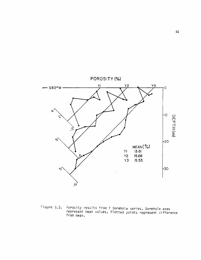
5.3 Porosity results from Y borehole series 44

vii

LIST OF ILLUSTRATIONS--continued.

Figure Page

5.4 Porosity results from Z borehole series 45

5.5 Scattergram plot of elevation vs LPDPER for alldata 48

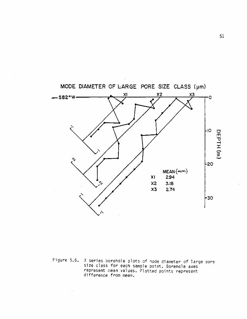
5.6 Mode diameter of large pore size class for Xborehole series 51

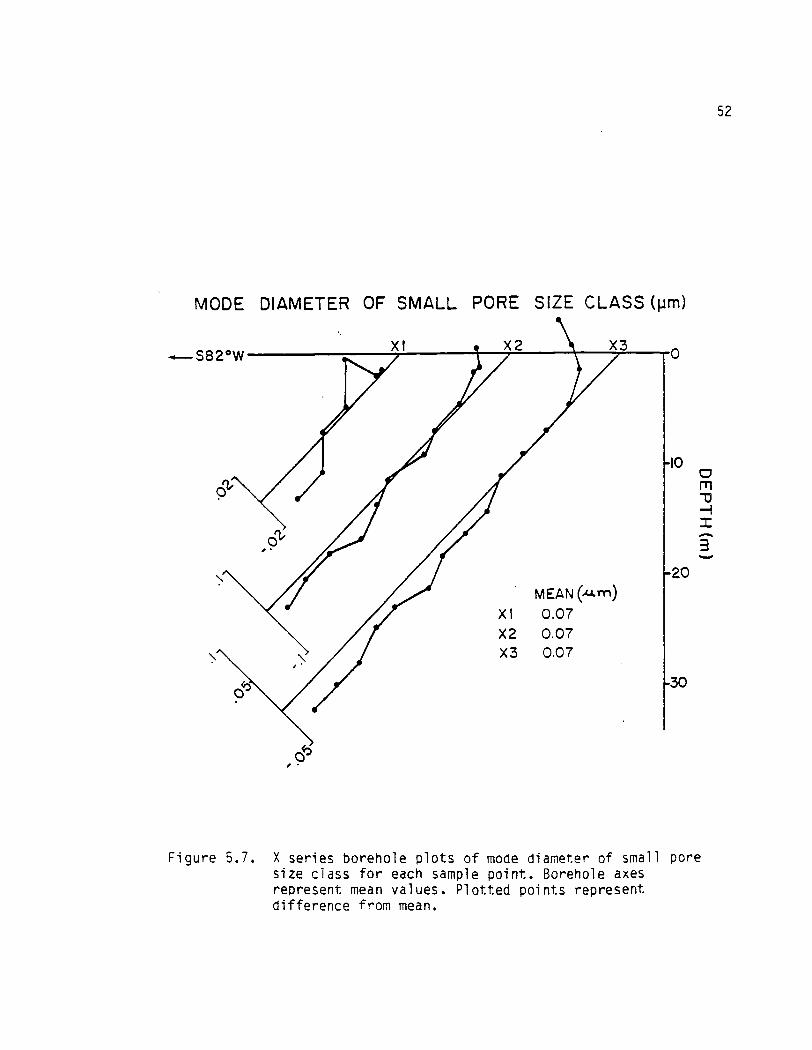
5.7 Mode diameter of small pore size class for Xborehole series 52

5.8 Mode diameter of large pore size class for Yborehole series 53

5.9 Mode diameter of small pore size class for Yborehole series 54

5.10 Mode diameter of large pore size class for Zborehole series 55

5.11 Mode diamter of small pore size class for Zborehole series 56

5.12 Pore with wide radius and throats with narrow radiileading into pore 58

5.13 Initial intrusion/extrusion plot of pore diametervs incremental intrusion volume 59

5.14 Second intrusion/extrusion plot pore diameter vsincremental intrusion volume 60

5.15 Five types of hysteresis loops describing differentpore arrangements 62

5.16 Capillary shapes which attribute to type Ehysteresis loops 63

5.17 Pore surface area results from X series boreholes 66

5.18 Pore surface area results from Y series boreholes 67

5.19 Pore surface area results from Z series boreholes 68

viii

LIST OF ILLUSTRATIONS--continued.

Figure Page

5.20 Plot of relative surface area and pore-sizedistribution vs pore diameter 70

5.21 Scattergram plot of LPDPER vs LPSAPER 71

5.22 Capillary wedge and adhesion of water on matrixparticle 73

5.23 Semi-variogram of bulk density data 76

5.24 Semi-variogram of porosity data 77

5.25 Semi-variogram of pore surface area data . . . . 78

5.26 Semi-variogram of mode diameter of large poresize class data 79

5.27 Semi-variogram of mode diameter of small poresize class data 80

5.28 Semi-variogram of porosity percentage from largepore size class data 81

5.29 Semi-variogram of pore surface area percentagefrom large pore size class data 82

5.30 Bulk density data from X series boreholes . . . 87

5.31 Bulk density data from Y series boreholes . . . . 88

5.32 Bulk density data from Z series boreholes . . . . 89

ix

LIST OF TABLES

Table Page

2.1 Borehole lengths 17

4.1 Pressure table used during intrusiton and extrusion 39

5.1 Statistical summary of porosity results 46

5.2 Statistical summary of porosity percentage fromlarge pore size class 49

5.3 Statistical summary of mode diameter of large poresize class 57

5.4 Statistical summary of pore surface area data . . 64

5.5 Semi-variogram results of spherical models . . . 83

5.6 Comparison of methods to determine bulk density . 85

5.7 Statistical summary of Magma Mine Road samples . 90

5.8 Statistical summary of brown zone and gray zonesamples 92

B1 Summary statistics of physical properties obtainedfrom core segments at the Apache Leap study site 110

B2 Summary of physical properties obtained from coresegments at the Apache Leap study site 111

B3 Summary statistics of pore area and pore-sizedistribution properties at the Apache Leap studysite 114

B4 Summary of pore area and pore-size distributionproperties at the Apache Leap study site . . . . 115

B5.1 Borehole X1 regression statistics 118

B5.2 Borehole X2 regression statistics 118

B5.3 Borehole X3 regression statistics 119

B5.4 All X series borehole data regression statistics 119

LIST OF TABLES--continued.

Table Page

B5.5 Borehole Y1 regression statistics 120

B5.6 Borehole Y2 regression statistics 120

B5.7 Borehole Y3 regression statistics 121

B5.8 All Y series borehole data regression statistics 121

B5.9 Borehole Zl regression statistics 122

B5.10 Borehole Z2 regression statistics 122

B5.11 Borehole Z3 regression statistics 123

B5.12 All Z series borehole data regression statistics 123

B5.13 All borehole data regression statistics 124

Cl Calibration results of poresizer 126

C2 Parameter comparison of two densely welded tuffsamples from the same location 127

xi

ABSTRACT

Characterization and quantification of fluid flow is dependent

upon the distribution, size and interconnectedness of pores in an

unsaturated rock matrix. This study examines the use of mercury

porosimetry in determining porosity, pore-size distribution and pore

surface area of an unsaturated, slightly welded to densely welded tuff

near Superior, Arizona. 121 samples of tuff were subjected to mercury

intrusion pressures to 200 MPa. A bimodal pore-size distribution exists

for all samples of slightly welded tuff with the larger pore size class

mode diameter averaging 2.91 pm and the lower pore size class mode

diameter averaging .07 11m. Interconnected porosity, pore surface area

and bulk density averaged 14.62%, 3.46 m 2 /gm and 2.13 gm/cm 3 ,

respectively. On average, 52.73% of the porosity was accounted for by

the large pore size class while 96.28% of the pore surface area was

accounted for by the small pore size class. Samples of densely welded

tuff exhibited a unimodal pore-size distribution with an average mode

diameter of .035 pm.

xii

CHAPTER 1

INTRODUCTION

The disposal of high-level nuclear waste into unsaturated,

fractured, consolidated media has recently received congressional

approval. The ability of the host rock to isolate high-level waste from

the accessible environment is of paramount importance. The rock matrix

near the repository has the potential to direct fluid movement away from

the repository to the surrounding environment. Fluid flow and transport

properties of the host rock must be thoroughly assessed before

repository operation is realized.

Characterization and quantification of fluid flow is dependent

upon the distribution, size and interconnectedness of pores in the rock

matrix. The matrix porosity indicates the fluid holding capacity of the

media while the pore-size distribution relates the fluid content as a

function of the matrix water potential. Unsaturated hydraulic

conductivity can be estimated from these relations. Pore size and

porosity also give indications of pore surface area. Specific surface

area measurements aid in sorption capacity estimates of the matrix by

quantifying available exchange sites.

In response to requisite research, the University of Arizona has

been contracted by the Nuclear Regulatory Commission to evaluate fluid

flow and transport through fractured, unsaturated tuff. Of particular

importance is the characterization of slightly welded tuff, similar to

that found at the Nevada Test Site. A field site near Superior, Arizona

1

2

has been set up to study slightly welded to densely welded tuff. The

Apache Leap study site is contained in slightly welded to non-welded

ash-flow tuff, approximately 3 km east of the town of Superior which is

located 50 miles east of Phoenix.

1.1 Rock Matrix Characterization

The unsaturated hydraulic conductivity and water holding capacity

are dynamic properties of the rock matrix which respond to the level of

stress present from temperature, loading and fluid availability. To

further estimation methods for unsaturated hydraulic conductivity and

water holding capacity, effective porosity and pore-size distribution of

the medium should be known. In this study, mercury porosimetry was

employed for the determination of porosity, pore-size distribution and

pore surface area. Mercury porosimetry relies on capillary theory and

the non-wetting property of mercury to determine porosity, pore-size

distribution and pore surface area by forcing mercury into matrix

samples under pressure. The instrument used in this study was capable

of intrusion pressures up to 200 MPa. Physical data consisting of bulk

and grain density can also be realized from this technique.

Samples are enclosed in a glass bulb attached to a capillary stem

known as a penetrometer (see figure 1.1). The sealed glass bulb and

stem are evacuated, filled with mercury and then subjected to

incremental pressure increases. The mercury responds by intruding into

smaller and smaller pores of the matrix sample. Mercury volume changes

in the penetrometer stem are directly related to intrusion volume and

3

Figure 1.1. Penetrometer assembly showing glass bulb and stem.

4

pore size according to capillary theory. Theoretically, pore sizes down

to 6 nm can be measured.

The intruded volume of mercury measures the interconnected pore

spaces of the matrix sample which includes conductive and dead end

pores. Pores > 6 nm in diameter were measured with the porosimeter used

in this study. Effective porosity determination from the water

saturation method measures all conductive and dead end pores. The

difference between the measured porosity from the porosimeter and

effective porosity from the saturation method is a function of the

porosity percentage accounted for by pore sizes less than 6 nm in

diameter in the matrix sample.

Incremental intrusion volumes are used to predict the pore-size

distribution range from atmospheric pressure to 200 MPa. Pore

geometries and arrangements can alter results predicted by capillary

theory by restricting fluid flow into pores. The effect is to

underestimate large pore sizes and overestimate small pore sizes. For

this reason, mercury porosimetry does not produce true pore-size

distribution curves. Pore sizes here are described by pore size classes

and the mode of the diameter of the pore size class to minimize the pore

geometry effects.

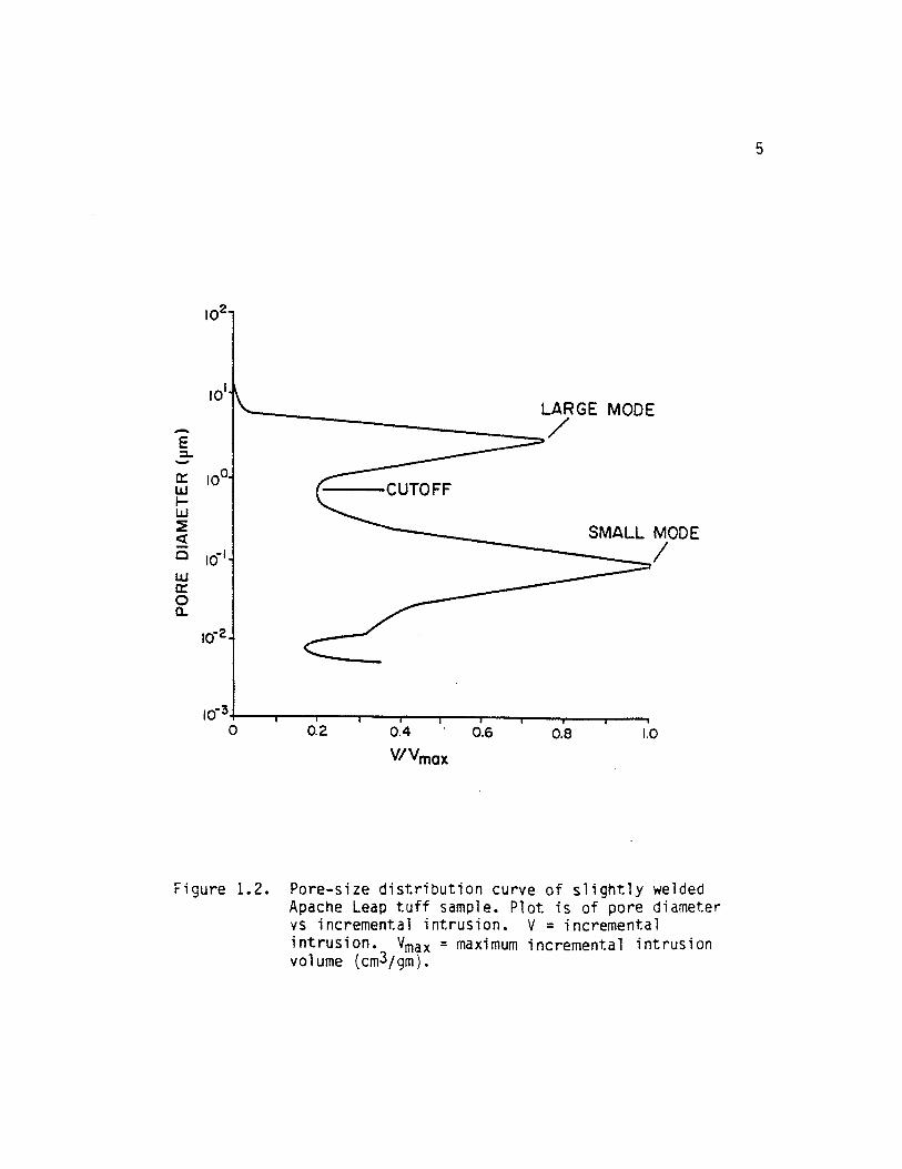
A typical pore-size distribution curve from the slightly welded

Apache Leap tuff is shown in figure 1.2. Two pore size classes are

evident from the plot of incremental pore volume versus pore diameter.

The minimum incremental intrusion volume pore diameter was chosen as the

cutoff between the two class sizes. The modes of each class size were

chosen to describe the bimodal distribution.

102-

5

LARGE MODE

CUTOFF

SMALL ,ODE

0 0.2I I

0:4 0.6 0.8 1.0

V/Vmox

Figure 1.2. Pore-size distribution curve of slightly weldedApache Leap tuff sample. Plot is of pore diametervs incremental intrusion. V incrementalintrusion. Vmax maximum incremental intrusionvolume (cm3/gm).

6

Porosity, pore-size distribution and pore surface area

measurements were performed on 105 matrix samples obtained from 9

boreholes inclined at an angle of 45 degrees at the Apache Leap site.

Sample locations were chosen at approximate 3 meter intervals along the

boreholes away from visible fractures.

Geostatistical methods were used to determine the spatial

variability of generated parameters along the boreholes and globally

throughout the study site area.

1.2 Objectives and Scope

This paper presents the findings of the initial study of physical

rock matrix properties from the Apache Leap study site. Fluid flow and

transport properties of the rock matrix are also being investigated by

others in the Department of Hydrology and Water Resources. The primary

objective is to characterize the matrix for fluid flow. More

specifically, the objectives of this study were to:

1) Determine porosity, pore-size distribution and pore surface area of

the rock matrix using mercury porosimetry.

2) Determine the spatial variability of these properties along each

borehole and globally throughout the study site location.

3) Compare different techniques to mercury porosimetry in the

determination of bulk density and porosity of the rock matrix.

4) Correlate generated data sets by regression analysis to determine

predictive capabilities of the analyzed parameters.

7

1.3 Other Related Work

In addition to mercury porosimetry studies of the rock matrix,

research continues on related matrix and fracture characterization.

According to Rasmussen and Evans (1986), bulk density and porosity of a

rock sample can be determined using water saturation, gravimetric and

gamma ray attenuation methods. Water saturation methods for porosity

are being investigated in the laboratory and caliper measurements of

rock volume, coupled with gravimetric analysis of sample weight are

being used for bulk density determination.

Rahi (1986) describes the outflow method to determine unsaturated

hydraulic conductivity, hydraulic diffusivity and moisture content. The

outflow method produces moisture characteristic curves between .01 and

.10 MPa suction. Research, in the laboratory, continues with the

outflow method on matrix samples 5 cm long by 6.35 cm in diameter.

Klavetter and Peters (1987) present moisture release curves

determined from thermocouple psychrometry. Research continues on 1 cm

by 1 cm unsaturated rock cylinders for suctions greater than 1 MPa.

Unsaturated pneumatic conductivity is being determined on the 5 cm by

6.35 cm cores mentioned above. The unsaturated pneumatic conductivity

is determined using the measured air flow, cross-sectional area and core

segment length in a sealed environment (Yeh et al., 1988).

Fracture orientation and characterization studies, along with

methods to analyze flux and travel times in fracture-matrix systems are

also being conducted. Groundwater recharge, infiltration and deep

percolation are being studied at a site adjacent to the field site.

Field data will be used to estimate boundary effects and fluxes over the

8

large-scale range of the hydrogeologic system when computer simulation

models are run. Also, existing field and laboratory techniques are

being scrutinized as to their applicability in the unsaturated fractured

rock.

Past and present research results will be analyzed to aid in the

characterization of the Apache Leap Tuff for matrix and fracture fluid

flow and transport.

CHAPTER 2

GEOLOGY AND FIELD SITE

2.1 Description of Study Area

The town of Superior lies in the northeast corner of Pinal County

Arizona. At an elevation of 910 meters, it is surrounded by the

Superstition Mountains to the northwest and Pinal Mountains to the east.

The Apache Leap is a 600 meter escarpment of ash flow tuff located just

east of the city. Queen Creek and its tributaries act as a major

drainage of the Apache Leap region. Queen Creek is a tributary to the

Gila River which is the major drainage for central and eastern Arizona.

U. S. Highway 60 is the major thoroughfare for the town of Superior. The

highway passes east through Queen Creek Canyon to the top of the Apache

Leap escarpment. Narrow canyons and pinnacles of weathered tuff are

ubiquitous along the roadcut and representative of the region.

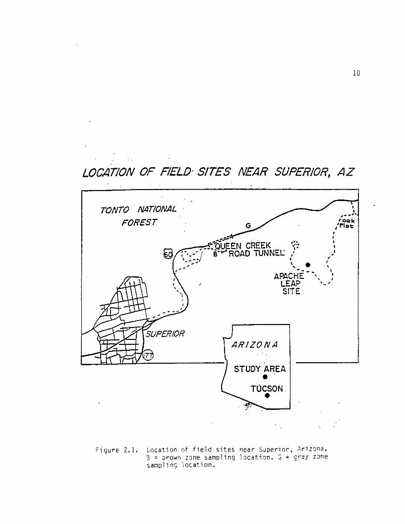
The Apache Leap Study Site is located on U. S. Forest Service

property south of highway 60 approximately 3 kilometers east of the town

of Superior (See figure 2.1). The study site was chosen as a field site

investigative area for unsaturated fractured tuff. The study site area

is contained in a much larger dacitic ash flow sheet extending areally

for approximately 250 km 2 .

9

1 0

LOCATION OF FIELD . SITES NEAR SUPERIOR, AZ

TONTO NATIONAL

FOREST • oa k;Plat •

--faijiEN CREEK 1:-12BROAD TUNNEL ,%

APACHE - "' s ,LEAP •- #SITE

ARIZONA

STUDY AREA•

TUCSON.

Figure 2.1. Location of field sites near Superior, Arizona.3 = Drown zone sampling location. G = gray zonesampling location.

11

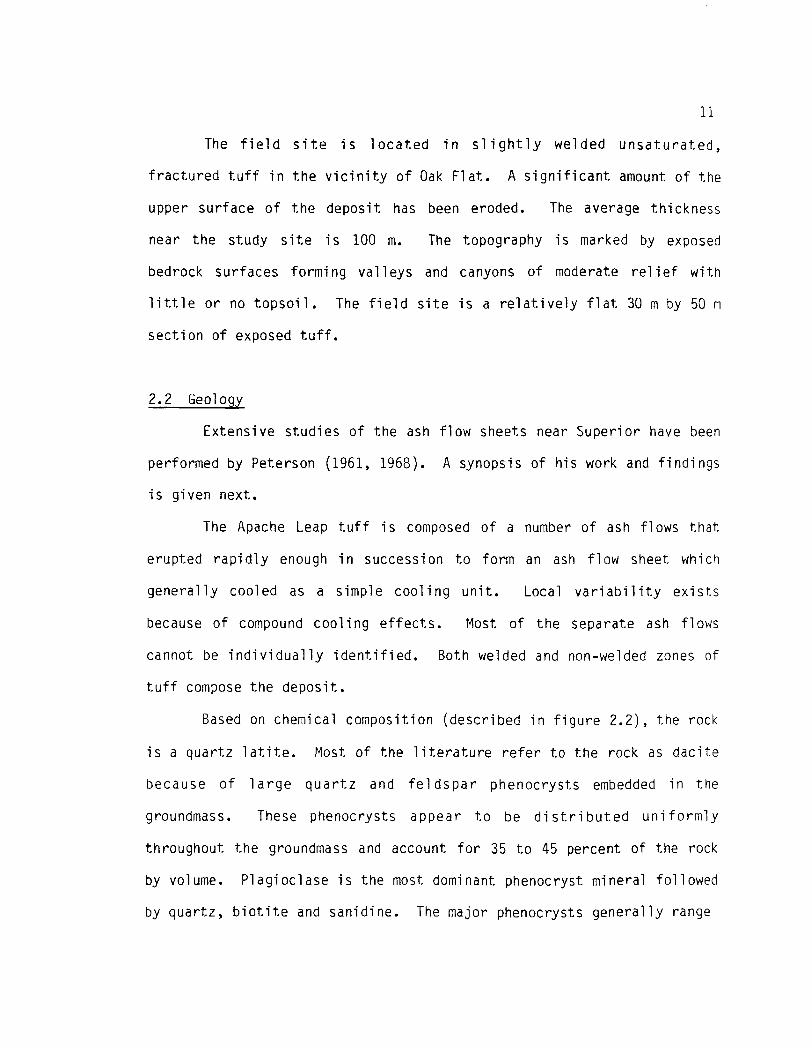
The field site is located in slightly welded unsaturated,

fractured tuff in the vicinity of Oak Flat. A significant amount of the

upper surface of the deposit has been eroded. The average thickness

near the study site is 100 m. The topography is marked by exposed

bedrock surfaces forming valleys and canyons of moderate relief with

little or no topsoil. The field site is a relatively flat 30 m by 50 m

section of exposed tuff.

2.2 Geology

Extensive studies of the ash flow sheets near Superior have been

performed by Peterson (1961, 1968). A synopsis of his work and findings

is given next.

The Apache Leap tuff is composed of a number of ash flows that

erupted rapidly enough in succession to form an ash flow sheet which

generally cooled as a simple cooling unit. Local variability exists

because of compound cooling effects. Most of the separate ash flows

cannot be individually identified. Both welded and non-welded zones of

tuff compose the deposit.

Based on chemical composition (described in figure 2.2), the rock

is a quartz latite. Most of the literature refer to the rock as dacite

because of large quartz and feldspar phenocrysts embedded in the

groundmass. These phenocrysts appear to be distributed uniformly

throughout the groundmass and account for 35 to 45 percent of the rock

by volume. Plagioclase is the most dominant phenocryst mineral followed

by quartz, biotite and sanidine. The major phenocrysts generally range

10%

GROUNOMASSPHENOCRYSTS

6011.

APACHE LEAP ruFF SITE

WHOLE ROCK ELEMENTAL COMPOSITION

50%

APACHE LEAP TUFF SITEMINERALOGICAL COMPOSITION

Figure 2.2. Elemental and mineralogical composition of ApacheLeap Tuff (After Peterson, 1961).

12

13

in size from .5 mm to 1 mm in diameter with occasional appearance of a 3

mm size.

Pumice fragments have also been identified in local abundance in

some parts of the deposit. Near the top of the deposit, they are

equidimensional but become more flattened in the lower zones of the

deposit. Most of the pumice inclusions carry the same phenocrysts with

the same proportions as the matrix. The difference lies in the fact

that unbroken phenocrysts appear in the pumice inclusions while the

phenocrysts in the enclosing rock are broken.

Ash flow tuff results from the deposition, compaction and

consolidation of a mobile, high-density suspension of hot glass shards,

pumice and rock fragments known as nuee' ardents. A flue& ardent is

both a type of eruption and an agent of transport consisting of a basal

avalanche and an overriding cloud of expanding gas and dust. The ash

flow sheets originated as nuee l ardents. The magma degassed with enough

explosive force to spread in all directions as a gas-charged avalanche.

The ash-sized particles were carried as far as 30 kilometers by the

basal avalanche.

The first material was quickly cooled on the pre-volcanic

Paleozoic limestone surface and formed an insulating layer which

prohibited rapid cooling of the subsequent flows. This insulating layer

is described as the lower non-welded zone in figure 2.3. It promoted

longer cooling and thus greater compaction and welding from the weight

of the overburden. The vitrophyre represents a layer of rapid cooling

and flattening, giving rise to a partly welded glass. Most of the

vitrophyre is a densely welded tuff composed of black glass and the

ZONES OF WELDING ZONES OFCRYSTALLIZATION

FIELD UNITS

Upper nonwelded [ f

ç.

-ae

••oxm

White

— — — —

Upper 1.....

Loaco.

Grayportly welded 3 ' u•0 1:›..c MIND •n• MMENI

t eM

0

Densely welded 1 cli* Brown

Lowerpartly welded [ Vitrophyre

Lower nonwelded [ Basal tuff

.

Figure 2.3. Physical characteristics of the Apache Leap Tuff(after Peterson, 1968).

14

15

normal distribution of phenocrysts. The vitrophyre ranges in thickness

from 1 m to 25 meters.

The deposit shows three color zones described by the degree of

welding in each layer. The brown unit cooled slower and the devitrified

glass formed an aphanitic groundmass of densely welded material. The

gray unit lies immediately above the densely welded brown unit and is

characterized by less welding (more porosity) and more crystallization

as the gases collected in the pore spaces. Near the top of the deposit,

as the gases filled even more pores and the weight of the overburden

decreased greatly, the particles remained undeformed and non-welded.

Crystallization dominated this white unit because of the constant flow

of gases up through the groundmass. The aphanatic groundmass of the

white unit lacks oriented structures. Its maximum thickness is 250

meters but only averages 60 to 100 meters in most locations.

The age of the tuff deposit has been confirmed to be of Tertiary

time. Dating techniques suggest a middle Miocene age, approximately 20

million years.

2.3 Borehole Description

Three sets of boreholes of varying lengths, each set in one

vertical plane, are located at the study site (See figure 2.4 ). The X

borehole set was drilled in September, 1985, while the Y and Z sets were

drilled in November, 1986. All three sets were drilled at a 45 degree

angle to the horizontal. Table 2.1 gives relevant information

concerning the length of all boreholes. A vertical datum was

established to a reference point located 14.14 m in the N37 ° E direction

„10m,...---.,

XI X2 X3 ,i— o —

Y1 Y2 ye? lom

Z3o ;!

Cover

Reference Point

PLAN VIEW

PROFILE VIEW

Figure :.4. Borehole configuration at the Apache Leap study siteshowing inclined boreholes. Thicker lines indicatelonger boreholes. All boreholes are nominally 10 cmin diameter.

16

17

from borehole X3. The borehole elevations are in reference to the lower

lip of casing on borehole X1 which was given an arbitrary elevation of

100 m.

TABLE 2.1 Borehole lengths. (after Weber, 1986)

BOREHOLE LENGTH (m)X1 18.4X2 32.6X3 46.6

Y1 17.2Y2 30.9Y3 44.9

Z1 17.0Z2 31.5Z3 45.2

The X and Y sets of boreholes trend in a westerly direction with

both X3 and Y3 being easternmost. The Z set trends in an easterly

direction with Z3 being westernmost. The X series of boreholes are

cased for 1.34 m below land surface while the Y and Z series are cased

for 1.58 m below land surface to maintain the integrity of the borehole

wall. The spacings are shown in figure 2.4.

Three dimensional fluid and transport monitoring is made possible

by this particular borehole configuration. The drilling procedure used

surface set HQ oversized diamond-core bits and a stabilizer equal to the

borehole diameter to maintain straight axi-symmetric drilling. Cores

with a diameter of 6.35 cm were obtained from the borehole. A scribing

tool provided a mark on the core every 3.05 m. This was done to provide

information on fracture location and orientation.

18

All core from the borehole drilling was logged. Weber (1986)

gives a description of fractures and their orientation of the X set of

boreholes. Fracture orientation and location data indicate steeply

dipping fractures which are generally directed to the southwest and

northwest. This is in good agreement with surface exposures of various

surrounding outcrops near the study area.

CHAPTER 3

BACKGROUND

Mercury porosimetry is based on capillary theory governing fluid

behavior. Previous studies have demonstrated its usefulness for a

variety of situations. Data have been collected and analyzed relying on

capillary and geostatistical theory, respectively.

3.1 Capillary Theory

The determination of the pore size distribution of porous media

using mercury porosimetry is a well established practice. Ritter and

Drake (1945) presented a paper fully devoted to mercury porosimetry,

which forms the basis of all present studies.

Washburn (1921) mentioned the idea of forcing mercury into a

porous material to obtain a pore size distribution. He drew upon the

relation:

P = -2 fi (cos a)/ r (3.1)

where P = pressure, e, = surface tension, a = contact angle and r = pore

radius, to determine the pressure required to force mercury into a pore

of radius r. Mercury is a non-wetting liquid toward most substances

with contact angle greater than 90 degrees. Therefore, it must be

forced into cracks or pores by applying pressure. From equation 3.1,

the required pressure is proportional to the surface tension of the

mercury and the cosine of the contact angle of the mercury on the solid

19

20

pore wall. Assuming pores to be cylindrical capillaries, equation 3.1

is used for the determination of pore size with mercury porosimetry.

Although this is not true in most naturally occurring porous media it

has been widely accepted as the standard. Studies by Joyner et al.

(1951) comparing mercury porosimetry to nitrogen desorption found good

agreement between the two methods.

For all data in this study, a contact angle of 130 degrees was

used for both intrusion and extrusion. A value of 485 dynes/cm was used

for the surface tension of the mercury meniscus. These values were

suggested by Micromeritcs Corporation (1986). A detailed description of

the procedure used in this study is contained in Appendix A.

During mercury intrusion, as the pressure increases mercury is

forced into smaller and smaller pores. Obviously the pores are not all

interconnected and of equal radius. Figure 3.1 shows shapes of grouped

pores. Because of pore heterogeneity and contact angle hysteresis, to

be discussed later, mercury will not be forced into pore radii as

predicted by equation 3.1. The group of pores in figure 3.1 do not act

as a single capillary or bundle of capillaries but as individual "ink

bottle" pores. With cylindrical constant radius pores, the governing

radius remains constant for intrusion and extrusion and equation 3.1

applies. With ink bottle pores, the throat radius controls intrusion

and the pore radius controls extrusion.

Given r n , the narrow radius of a pore neck and rw , the wide pore

radius, it is seen that rn is the governing radius during intrusion. As

pressure increases mercury is forced into smaller pores. Figure 3.1.a

shows a situation where this is not absolutely true. As the pressure is

Figure 3.1. Grouped pores of varying radii.

Figure 3.1.a

Pore with narrowthroat radius andwide pore radius.

Figure 3.2.

Dead end pore withrestricting throat.

21

22

increased up to some value Pn corresponding to rn, the pore neck will be

intruded with mercury. The intrusion will continue until all of the

pore is filed because Pw , the pressure associated with a pore of radius

rw , has been exceeded.

The opposite occurs during extrusion. Some pressure Pmax has

been attained at the upper limit of intrusion and then the pressure is

decreased to a value equal to P n . The mercury in the pore will not

leave the pore until a value of Pw is reached. If Pn >> Pw and

subsequently rw >> rn then it is possible that mercury cohesive forces

will be broken and a discontinuity in the mercury stream will result

causing mercury to be trapped in the pore. This is termed volume

hysteresis. Kloubek (1981) suggests no discontinuities will occur but

that mercury will still be trapped in the pore.

Volume hysteresis may be a function of several factors including:

1)pore geometry; 2)pore roughness; 3) ink bottle effect; 4) surface

tension variability; and 5) contact angle hysteresis. Contact angle

hysteresis is defined as the change in angle of contact between

intrusion and extrusion. Contact angle values vary according to the

material being intruded. Kloubek (1981) and Good and Mikhail (1981)

found values as high as 180 degrees for advancing (intruding) angles and

values as low as 90 degrees for receding angles. The advancing angle is

generally greater than the receding one.

Volume hysteresis can also arise due to the ink bottle effect.

In the case of dead end pores as illustrated in figure 3.2, the smaller

the ratio of rn :rw the larger the difference between intrusion and

23

extrusion pressures. If the ratio is low enough, according to Kloubek,

mercury will remain trapped in the pore regardless of the neck size.

The initial intrusion/extrusion produces volume hysteresis. When

subsequent pressure increase/decrease takes place/ the curves are shaped

differently (see figures 3.3 and 3.4). The newly shaped reintrusion

curve defines local hysteresis. Kloubek (1981) stated that the local

hysteresis was caused by mercury caps being formed on the already-filled

pores. The change in volume of these caps is a function of their

curvature. It is assumed that the mercury menisci do not move along the

pore wall during reintrusion.

In comparing saturation/desaturation curves of water and mercury

for different pore arrangements, certain similarities exist. For the

simplified pore geometry of figure 3.5 when rn :rw is sufficiently high,

the behavior of water and mercury is shown in the figure. Mercury

saturation is attained at some pressure P n , while water saturation is

attained at Sw , or near zero relative suction. In this ink bottle

example, water will be drawn out of the pore when the threshold suction

value, Sn , corresponding to r n occurs. Theoretically, the pore will

rewet upon reaching some suction value S.

This phenomenon is in direct comparison to the volume hysteresis

mentioned earlier. The mercury intrusion curves are a better

representation of water desorption than the extrusion curves. In the

case of mercury intrusion, larger pores fill first under a low pressure.

As the pressure is increased, smaller and smaller pores are filled with

mercury until some maximum pressure is attained. The controlling radius

upon intrusion is the size of the throat leading into a pore. With

24

1 02

EXTRUSION

1

1INTRUSION

10-3 . III II I0 0.2 0.4 0.6 0.8 1.0

V/Vm

Figure 3.3. Initial intrusion/extrusion plot of pore diameter vscumulative intruded volume of Hg (cm3 /gm). Vm = totalvolume intruded. V = cummulative intruded volume.

n%.,.

.....

.....

...,N.

Nn. EXTRUSION

NN\

%. n

1 Q 2

I

.to- -..

INTRUSION

.

N\II

25

I 1 I 1 11 11 1 1

0 0.2 0.4 0.6 0.8 1.0

V/ Vm

Figure 3.4. Second intrusion/extrusion plot of pore diameter vscumulative intruded volume of Hg (cm3 /gm). Vri = totalvolume intruded. V = cumulative intruded volume.

> AC-

A

MERCURYWATER

esat esot

WATER HgA

> >PWPRESSURE—n

SW

SUCTION-

SN PN

26

Figure 3.5. Dead end pore and theoretical behavior of water andmercury with pressure/suction increase and decrease.

27

water desorption, the large pores drain first under low suction or

tension. As the suction increases, smaller and smaller pores are

drained of water. The controlling radius in this case is again the

throat size connecting pores. If a situation exists like figure 3.5,

then the large pore will not drain until a suction value corresponding

to the smaller throat radius is reached. For these reasons, mercury

intrusion should be considered comparable to the water desaturation

curves when comparing results between the two methods.

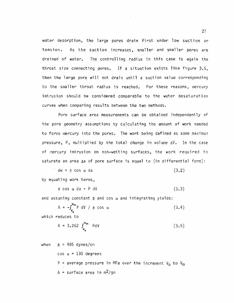
Pore surface area measurements can be obtained independently of

the pore geometry assumptions by calculating the amount of work needed

to force mercury into the pores. The work being defined as some maximum

pressure, P, multiplied by the total change in volume V. In the case

of mercury intrusion on non-wetting surfaces, the work required to

saturate an area Aa of pore surface is equal to (in differential form):

dw = (3 cos a da (3.2)

By equating work terms,

f3 cos a da = P dV (3.3)

and assuming constant (3 and cos a and integrating yields:

A = -flVf m P dV / (3 cos a (3.4)0

which reduces to

A = 3.262 fvm PdV (3.5)v.

when B = 485 dynes/cm

cos a = 130 degrees

P = average pressure in MPa over the increment Vo to Vm

A = surface area in m2/gm

28

Vo = cummulative intruded pore volume at Po in cm3/gm

Vm = cumulative intruded pore volume at Pm in cm3/gm

Rootare and Prenzlow (1967) found good agreement with mercury

intrusion and gas adsorption techniques on materials with areas below

100 m2 /gm.

3.2 Previous Work

Since the mercury porosimetry study of Ritter and Drake (1945),

mercury porosimetry has been widely used in industry. Its applications

have varied from the study of pore structure and fluid distributions by

Pickell et al. (1965) to a recent study by Klavetter and Peters (1987)

regarding hydrologic properties of volcanic tuff.

Winslow and Lovell (1981) measured pore size distributions of a

variety of construction materials including portland cement, compacted

fine grained soils and shales using mercury intrusion. Whittemore

(1981) used mercury porosimetry to obtain pore size distributions in

ceramic processing research. Both raw materials and finished products

were subjected to mercury porosimetry measurements to measure structure.

Klar (1971) used porosimetry to study the changes in inter and intra

particle porosity for copper powder as a function of compacting

pressure.

A similar application of mercury porosimetry to this study was

performed by Klavetter and Peters (1987). They compared mercury

intrusion saturation curves to thermocouple psychrometer saturation

curves from samples of welded and non-welded tuff. They found good

agreement between the two methods for a small number of samples but

29

overall agreement was poor. A large variability was found in the

mercury intrusion results. It should be pointed out that comparison of

mercury intrusion was made with psychrometer saturation curves. Perhaps

a more favorable result would have been attained if desaturation curves

had been compared.

According to Klavetter and Peters (1987), the pore size

distribution results using mercury intrusion of the welded and slightly

welded tuffs qualitatively agreed with the results from scanning

electron microscopy. They also found pore size distributions from

mercury porosimetry results capable of measuring larger pore diameters

more accurately than thermocouple psychrometry.

An excellent bibliography on mercury porosimetry was presented by

Modry et al. (1981).

3.3 Geostatistical Theory

The geostatistics methodology began in the mining industry to

estimate ore reserves. Matheron (1973) provided a theoretical basis by

the formation of random functions. The method resembles the classical

statistical approach but differs by assuming that adjoining samples are

correlated spatially instead of being independent of each other. The

appeal here is the recognition of the spatial relationship and its

ability to be expressed in quantitative terms. This correlation can be

expressed in terms of a function known as a variogram.

The following explanation draws upon literature by Kim (1981) and

Warrick et al. (1986).

30

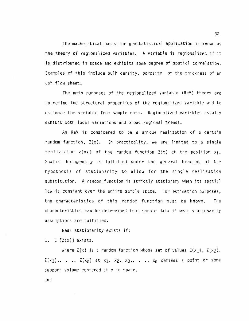
The mathematical basis for geostatistical application is known as

the theory of regionalized variables. A variable is regionalized if it

is distributed in space and exhibits some degree of spatial correlation.

Examples of this include bulk density, porosity or the thickness of an

ash flow sheet.

The main purposes of the regionalized variable (ReV) theory are

to define the structural properties of the regionalized variable and to

estimate the variable from sample data. Regionalized variables usually

exhibit both local variations and broad regional trends.

An ReV is considered to be a unique realization of a certain

random function, Z(x). In practicality, we are limited to a single

realization z(xi) of the random function Z(x) at the position xi.

Spatial homogeneity is fulfilled under the general heading of the

hypothesis of stationarity to allow for the single realization

substitution. A random function is strictly stationary when its spatial

law is constant over the entire sample space. For estimation purposes,

the characteristics of this random function must be known. The

characteristics can be determined from sample data if weak stationarity

assumptions are fulfilled.

Weak stationarity exists if:

1. E [Z(x)] exists.

where Z(x) is a random function whose set of values 7(x1), Z(x2),

7(x3),. . L(x) at xi, x2, x3,. . xn defines a point or some

support volume centered at x in space,

and

31

2. For any vector h, the variance of Z(x+h) - Z(x) exists and depends

only on h.

Weak stationarity is also known as the intrinsic hypothesis. The

intrinsic hypothesis does not fulfill second order stationarity

assumptions, however. Second order stationarity exists when:

1. E[Z(x)] exists and does not depend on x.

2. For each pair of random variables, [Z(x), Z(x+h)] the covariance,

C(h), exists and does not depend on x.

C(h) = E[Z(x) Z(x+h)] - m 2 (3.6)

where m = mean value or E[Z(x)]

The variogram function defines the spatial correlation of adjoining

samples and only requires weak stationarity. This correlation is the

structured aspect of ReV and also of the random function. The variogram

(h) is defined as:

7(h) = 0.5 Var[Z(x) - Z(x+h)] (3.7)

where x is defined as above and h is some distance away from x. "Var"

here is the variance. Assumming zero drift, E[Z(x+h)] = E[Z(x)] and

equation 3.7 is equal to

2 7 (h) = E[Z(x) - Z(x+h)]2 (3.8)

An estimate of 7(h) or 7 * (h) is given by:

7* (h) = 0.5 (1/n) 1 7E1 [Z(xi) - Z(x1+h)1 2 (3.9)

with n being the number of pairs separated by some distance h. This is

a vector function of the distance h.

A typical variogram is given in figure 3.6. The lag distance, h,

is the separation distance between sample pairs. The range, r, is

32

defined as the distance at which sample pairs are correlated. The value

of 7(r) is called the sill. If h > r, samples are no longer

correlated. Sometimes the value of 7(0) does not equal zero. This is

termed the nugget value C o . It is used to characterize the residual

influence of all variabilities which have ranges much smaller than the

available distances of observations. In general the nugget value should

be small if proper sampling procedures have been followed.

LAC; DISTANCE ( 11 )

Figure 3.6. Semi -variogram showing sill, range, r, and nugget Co.

CHAPTER 4

SAMPLE DESCRIPTION AND PROCEDURES

Samples were collected and analyzed according to the following

information. General procedural guidelines were supplied by

Micromeritics Corporation (1986).

4.1 Sample Description

Approximately 285 m of 6.35 cm diameter core resulted from the

borehole drilling. Figure 4.1 shows the borehole arrangement and sample

locations. A sampling scheme was implemented to test an equal number of

samples from each borehole set. As a result of this scheme, 35 sample

points were chosen for each set with seven samples originating from the

shortest boreholes (Xl, Y1 and Z1), 12 samples from each borehole X2, Y2

and Z2 and 16 samples from the longest boreholes (X3, Y3 and Z3).

Sample points are given letter designations in figure 4.1.

Sample points in the top four meters of core were chosen at

approximately 1 m intervals. This was done to better define any surface

effects of the deposit. At points below four meters in all boreholes,

samples were chosen at approximately 3 m intervals. Together 105 sample

locations were chosen and cut from the original core. Sample locations

were purposely chosen away from any visible fractures in the core,

causing non-uniform spacing between sample points. A 10 cm length of

core was cut for each sample location. The top 5 cm portion was used

33

34

APACHE LEAP TUFF SITE

CORE SAMPLE LOCATIONS

Figure 4.1. Apache Leap study site sample locations. Letterdesignations indicate sample points. 105 points total.

35

for another study involving air and water permeability and thermal

conductivity. The next 2.5 cm portion was used for this study while the

last 2.5 cm portion was used for psychrometry investigations. Figure

4.2 details the 10 cm core segment.

The 10 cm core samples were cut using a water cooled diamond

radial arm rock saw. Maximum dimensions for samples in this study were

2.5 cm in diameter by 2.5 cm long. A diamond edged coring bit 2.54 cm

in diameter was used to drill the samples out of the original core. All

samples were sized from 2 cm to 2.5 cm long.

Once the samples were cut to proper dimensions they were dried at

105 degrees C until weight loss ceased. They were then placed in sealed

containers until porosimetry measurements were performed.

4.2 Poresizer Description

The instrument used in this study was a Micromeritics Model 9310

Poresizer capable of intruding mercury up to 200 MPa. A Welch

Scientific Model 1402 vacuum pump capable of 1 x 10 -4 mm Hg was used in

conjunction with the poresizer. An IBM PC computer linked the software

supplied by Micromeritics to the poresizer.

The poresizer measures the volume of mercury intrusion and

extrusion on an electrical capacitance basis. The volume of mercury

forced into the pores of a sample by an applied pressure is measured by

the change in electrical capacitance of a cylindrical coaxial capacitor

formed by an outer metallic shield on the penetrometer stem and the

inner column of mercury. As pressure is increased and mercury

14-L.6 cm

other uses

Mercury Intrusion— Bulk a Grain Density— Effective Porosity— Pore Size Distribution— Pore Area

1cm

other usesI cm

36

Figure 4.2. Ten cm borehole core segment and its uses.

37

is forced into the sample pores, the level of mercury falls in the

penetrometer stem causing a linear decrease in electrical capacitance.

Figure 1.1 diagrams the type of penetrometer used. Each

penetrometer has associated with it a calibration factor in units of

microliters per picofarad. Capacitance changes are converted to volume

changes by multiplying by the appropriate calibration factor. Both the

inner and outer diameters of the penetrometer stem are carefully

controlled to detect volume changes of well under one microliter. The

glass stem of the penetrometer is made of metal-clad precision-bore

borosilicate glass capillary tube which is fused to a chamber which

contains the sample.

Samples are loaded into the glass chamber of the penetrometer,

sealed and then evacuated to a vacuum near 50 pm of Hg. Mercury is

loaded into the penetrometer through a capillary in the stem. As

mercury flows into the penetrometer, it surrounds the sample and fills

the capillary in the penetrometer stem. Low pressure mercury intrusion

can be detected between 0 MPa and atmospheric pressure. In this study,

pore size corresponding to below atmospheric pressure was not

significant. Therefore, only high pressure intrusion/extrusion results

are reported.

High pressure generation is accomplished in the poresizer with a

ram driven by a ball screw which is driven by a gear motor. The high

pressure system is filled with high pressure fluid (a mixture of

synthetic oil and low-odor kerosene) which is pressurized by the ram.

This fluid contacts the mercury capillary in the penetrometer stem and

forces the mercury into the pores. A capacitance transducer connected

38

to the high pressure chamber via a gold-plated banana plug and conical

insulator detects and measures the intrusion volume.

4.3 Procedure

A complete listing of the procedures used for mercury intrusion

is given in Appendix A. A general description follows.

Once the samples were dried, weighed and loaded into the

penetrometer they were evacuated and then surrounded by mercury.

Samples in the penetrometer were subjected to a range of pressures from

atmospheric to near 200 MPa. Pore sizes corresponding to pressures

below atmospheric pressure were considered insignificant because initial

intrusion commenced at pressures close to twice atmospheric. A listing

of the pressure table used in this study is given in Table 4.1. Each

sample was subjected to one intrusion/extrusion cycle per run. Two runs

were performed on each sample. This was done for two reasons: 1) to

better define the volume hysteresis effect of the various pore sizes;

and 2) to quantitatively analyze the effect of pore size on trapping

mercury. During the high pressure test, pressure equilibrium was

established for ten seconds for each pressure point in table 4.1 before

a reading was recorded. This allowed time for mercury equilibrium

within the pores.

Intrusion/extrusion data were recorded and stored automatically

on the PC. At the completion of each test, the results were stored on

a data diskette. Direct parameter listings of total intrusion volume,

pore area, median pore diameter, bulk density and skeletal density were

stored. From this information, porosity was determined by multiplying

39

the total intrusion volume by the bulk density. Pore size distribution

was determined by plotting the incremental pore volume versus pore

diameter using equation 3.1.

TABLE 4.1 Pressure table used during automatic high pressure operationof Poresizer 9310. Only intrusion pressures are shown. Extrusionpressures are the same as intrusion values only in the reverse orderi.e. from 163 MPa to .10 MPa. Pore diameter intruded is according tocapillary theory and equation 3.1.

PORESIZER PRESSURE(MPa) (psia)

PORE DIAMETER INTRUDED(um)

.10 14.7 12.2

.13 18.9 9.52

.17 24.1 7.46

.21 30.8 5.84

.27 39.4 4.57

.35 50.4 3.57

.44 64.4 2.79

.57 82.6 2.18

.72 105 1.71

.93 135 1.331.19 172 1.051.52 221 .821.95 283 .642.48 360 .503.19 462 .394.07 590 .315.20 754 .246.64 963 .198.49 1231 .1510.8 1574 .1113.9 2018 .0917.8 2580 .0722.7 3300 .0529.1 4220 .0437.2 5390 .0347.6 6910 .02660.9 8830 .0277.9 11300 .016

100 14500 .012127 18450 .0098163 23600 .0076187 27200 .0066

CHAPTER 5

RESULTS AND DISCUSSION

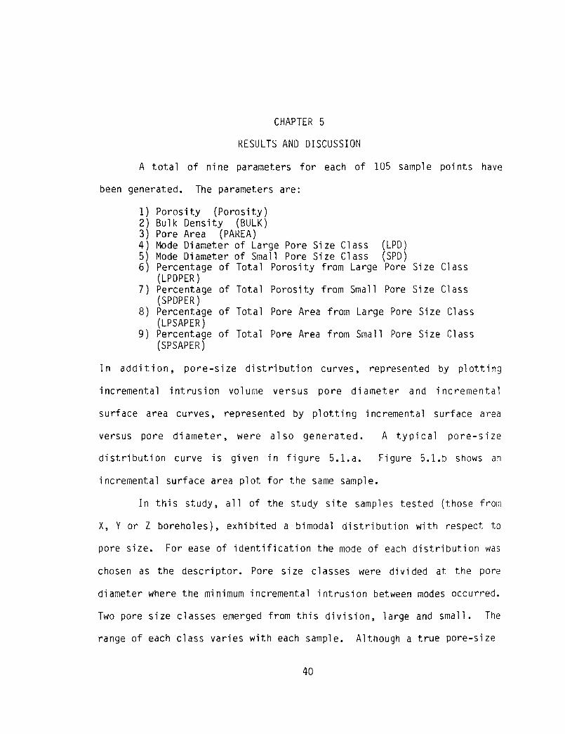
A total of nine parameters for each of 105 sample points have

been generated. The parameters are:

1) Porosity (Porosity)2) Bulk Density (BULK)3) Pore Area (PAREA)4) Mode Diameter of Large Pore Size Class (LPD)5) Mode Diameter of Small Pore Size Class (SPD)6) Percentage of Total Porosity from Large Pore Size Class

(LPDPER)7) Percentage of Total Porosity from Small Pore Size Class

(SPDPER)8) Percentage of Total Pore Area from Large Pore Size Class

(LPSAPER)9) Percentage of Total Pore Area from Small Pore Size Class

(SPSAPER)

In addition, pore-size distribution curves, represented by plotting

incremental intrusion volume versus pore diameter and incremental

surface area curves, represented by plotting incremental surface area

versus pore diameter, were also generated. A typical pore-size

distribution curve is given in figure 5.1.a. Figure 5.1.b shows an

incremental surface area plot for the same sample.

In this study, all of the study site samples tested (those from

X, Y or Z boreholes), exhibited a bimodal distribution with respect to

pore size. For ease of identification the mode of each distribution was

chosen as the descriptor. Pore size classes were divided at the pore

diameter where the minimum incremental intrusion between modes occurred.

Two pore size classes emerged from this division, large and small. The

range of each class varies with each sample. Although a true pore-size

40

SMALL MODE

102-

0:4 0.6 0:8 1.0

V/VMOX

Figure 5.1.a Pore-size distribution curve of sample CC. Plot is ofpore diameter vs incremental intrusion. V= incremental intrusion

Vmax = maximum incremental intrusion volume (cm3 /gm).

10-3o

0.4

V/Vm

Figure 5.1.b Plot of pore diameter vs incremental surface area forsample CC. V = incremental surface area. Vm . maximumincremental surface area (m2 /gm).

0.6 0.8 1.0

101

LARGE MODE//

41

42

distribution is not given here, one can get an idea of the pore size

range by looking at the two modes and the percentage of porosity and

surface area from each pore size class. Numbers 4) and 5) above

represent the mode of the individual class size. Numbers 6) and 7)

represent the percentage of total porosity attributed to the respective

pore size division. Numbers 8) and 9) represent the percentage of pore

area attributable to each pore size class.

All of the data generated in this study is found in Appendix B.

Relevant data will be presented in tabular and graphical form throughout

the discussion. Regression statistics can also be found in Appendix B.

Calibration results for the porosimeter are found in Appendix C. The

porosimeter was checked for intrusion volume accuracy every 50 sample

measurements. Manufacturer supplied silica-alumina pellets with a known

pore volume and surface area were the calibration standard.

5.1 Porosity

Porosity determinations based on mercury porosimetry are limited

to the maximum attainable pressure applied by the poresizer. The

maximum pressure attained in this study was 200 MPa. According to

equation 3.1, a pore diameter of 6 nm can be intruded at this pressure.

Figures 5.2 to 5.4 show porosity of each borehole sample. The axis of

the borehole represents the mean porosity value for each individual

borehole. Table 5.1 gives a summary of the porosity statistics.

The porosity results represent measurable interconnected porosity

of the tuff samples to a pore size of 6 nm. Interconnected porosity

accounts for both dead end pores and liquid conducting pores. These

POROSITY (%)x I X2S 82° W X3

0

20

MEAN (%)XI 12.95X2 14.54X3 14.18

30

43

.7 igure 5.2. Porosity results from X borehole series. Borehole axesrepresent mean values. ?lotted points representdifference from mean.

0

MEAN(%)YI 13.81Y2 15.08Y3 15.55

30

Figure 5.3. Porosity results from Y borehole series. Borehole axesrepresent mean values. Plotted points represent differencefrom mean.

44

Z1 13.05Z2 16.91Z3 13.87

45

Figure 5.4. Porosity results from Z borehole series. Borehole axesrepresent mean values. Plotted points represent

difference from mean.

46

values are from first run intrusion results. In some instances, a small

volume of mercury was intruded into new pores during the second

intrusion run. This amount never amounted to over two percent of the

total porsity. It is questionable whether this newly intruded mercury

actually measured matrix porosity or just some breakdown or destruction

of the microporosity of the sample. For this reason, only first run

porosity is considered.

TABLE 5.1 Statistical summary of porosity results. Mean values in %of measured porosity. Total number of samples equals 105.

BOREHOLE MEAN VARIANCE COEF. OF SKEW COEF. OF VARIATIONX1 12.95 1.99 .13 .11X2 14.54 5.61 -.99 .16X3 14.18 2.38 .55 .11

ALL X 14.06 3.56 -.17 .13

Y1 13.81 3.87 .24 .14Y2 15.08 4.78 .18 .14Y3 15.55 4.94 .86 .14

ALL Y 15.04 4.71 .51 .14

Z1 13.05 2.73 .74 .13Z2 16.91 96.73 3.25 .58Z3 13.89 4.39 -.66 .15

ALL Z 14.75 35.28 4.99 .40

ALL DATA 14.62 14.67 6.15 .26

Klavetter and Peters (1987) determined porosity on samples of

tuff from Yucca Mountain in Nevada and concluded that pressures in

excess of 345 MPa must be employed to measure interconnected porosity.

The porosity values here will be less than actual porosity. Because of

sample variation, an estimated difference between actual porosity and

measured porosity is not available. Later in this discussion the

mercury intrusion porosity results will be compared to water saturation

47

method results. The comparison will give a quantification to the pore

space < 6 nm.

Tables B5.1 - 13 (in Appendix B) contain statistical data on

individual boreholes, the X, Y and Z series boreholes and all borehole

data. Included are correlation coefficients, covariance and cross-

product results from regression of each parameter versus every other

parameter, including elevation.

Figure 5.2 shows the variation of porosity with depth along the X

boreholes. X1 shows the strongest correlation with elevation at -.78.

The correlation coefficient suggests porosity is increasing with depth

along the borehole. Grouping all of the X boreholes, results in a

correlation with elevation of -.56. Although this is not a strong

linear regression coefficient it does suggest an increasing porosity

trend with depth. A decreased porosity near the surface of the deposit

is likely due to chemical and physical weathering of the formation. The

probable increased crystallization of minerals in fractures and pores

certainly could affect the porosities of the samples. Surveying the

regression statistics from all of the data in table B5.13 shows a minor

correlation between depth and porosty of -0.26. This suggests the X

borehole set possibly can be accounted for by local variation and not

totally representative of the study site.

A more interesting result is obtained when regressing the

porosity percentage from the large pore size class (LPDPER) versus

elevation. Table 5.2 gives a synopsis of the information. More of the

porosity is accounted for by the large pore size class with depth along

the boreholes. A scattergram plot of the porosity percentage from the

48

100 • it x

.." z.

x.

so „

xl

70

eso 10 20 30 40 50 60 70 80

POROSITY PERCENTAGE FROM LARGE PORE SIZE CLASS (LPDPER),

Figure 5.5. Scattergram plot of elevation vs percentage of porosity

accounted for by the large pore size class (LPDPER). Xseries data plotted with I lr l ; Y series with '+'; and Zseries with 'x'.

90

49

large pore size class (LPDPER) versus elevation is contained in figure

5.5. Samples from the X, Y and Z series are represented by *, + and x,

respectively. The volume of larger pores increases with depth. Again,

surface effects may play a part in this phenomenon. Two separate

regressions were performed on the data in figure 5.5. A regression

coefficient of -.59 resulted when elevation was regressed against LPDPER

considering only data between 90 and 100 m in elevation. A regression

of data from 65 to 90 m in elevation produced a -.11 regression

coefficient. These coefficients suggest a definite surface effect on the

large pore size class porosity percentage. As the deposit cooled, gas

filled pores in local abundance toward the top of the deposit causing

larger pore sizes.

TABLE 5.2 Sample statistics for percentage of porosity from the largepore size class (LPDPER). Correlation coefficient is of elevationversus LPDPER. Mean values are in percent of measured porosity. Totalnumber of samples equals 105.

BOREHOLE MEAN VARIANCE COEF. OF SKEW CORRELATION COEF.

X1 45.16 53.34 -1.11 -.459X2 52.98 157.6 -.89 -.783X3 51.87 118.7 -1.49 -.687

ALL X 50.91 121.5 -.79 -.687

Y1 56.95 161.6 .31 -.922Y2 49.29 299.0 -.94 -.757Y3 51.85 572.5 -1.56 -.726

ALL Y 51.99 385.5 -1.40 -.638

7 1 44.89 160.2 .42 -.954Z2 57.82 227.9 .65 -.779Z3 57.96 70.9 -.03 -.565

ALL Z 55.29 161.2 .21 -.656

ALL DATA 52.74 221.9 -1.09 -.628

50

Near the surface of the deposit the ash flow cooled quickly

releasing its trapped gas, allowing for smaller particle crystallization

and less porosity. The trapped gas increased with depth up to a certain

point allowing for larger pore sizes but not greater porosity. Slightly

more than 50% of the porosity is accounted for by the large pores when

considering all sample points.

5.2 Pore-Size Distribution

One major advantage to mercury porosimetry is the relative ease

and time required to obtain a pore-size distribution. Figures 5.6 to

5.11 show the modes of the large and small pore size classes along the

borehole axes.

Overall, no strong correlation exists between the modes of the

bimodal distributions and any of the other parameters. Individual

borehole results can be found in tables B5.1 - 12. The mode diameter of

the small poresize class (SPD) exhibits a strong positive correlation

with elevation in the X and Z series boreholes, .743 and .699,

respectively but shows almost no correlation in boreholes Y2 and Y3.

For most data, except Y2 and Y3, the mode diameter for the small pore

size class decreases with depth which correlates with the occurrence of

larger pore sizes with depth discussed earlier. Table 5.3 describes the

sample statistics of the distributions.

The relatively small variance for both parameters indicates that

most samples are grouped near the mean and that the deposit is fairly

homogeneous with respect to the individual pore size classes.

MODE DIAMETER OF LARGE PORE SIZE CLASS (pm)XI X2 X3

-.— S82°W

MEAN (Mi)XI 224X2 3.18X3 2.74

51

Figure 5.6. X series borehole plots of mode diameter of large poresize class for each sample point. Borehole axesrepresent mean values. Plotted points representdifference from mean.

MODE DIAMETER OF SMALL PORE SIZE CLASS (pm)

0

MEAN (44m)

X I 0.07X2 0.07X3 0.07

-30

Figure 5.7. X series borehole plots of mode diameter of small poresize class for each sample point. Borehole axesrepresent mean values. Plotted points representdifference from mean.

52

MEAN (1-01-1)

'n 3.65Y2 3.10Y3 2.10

30

MODE DIAMETER OF LARGE PORE SIZE CLASS (urn)Y I Y2 Y3 .--S8 2°W 0

Figure 5.8. Y series borehole plots of mode diameter of large poresize class for each sample point. Borehole axesrepresent mean values. Plotted points representdifference from mean.

53

-0-- S 82°W 0

MEAN (Lsan)Y I 0.06Y2 0.07Y3 0.05

30

MODE DIAMETER OF SMALL PORE SIZE CLASS (pm)

Figure 5.9. Y series borehole plots of mode diameter of smallpore size class for each sample point. Borehole axesrepresent mean values. Plotted points representdifference from mean.

54

MODE DIAMETER LARGE PORE SIZE CLASS (pm)

Z3 Z2 Z1-r-S8 2°W 0

MEAN (04Arn)

Z1 3.37Z2 3.15Z3 2.81

Figure 5.10. Z series borehole plots of mode diameter of largepore size class for each sample point. Borehole axesrepresent mean values. Plotted points representdifference from mean.

55

MODE DIAMETER SMALL PORE SIZE CLASS (pm).---S82°W 0 Z3 Z2 Z I

MEAN(.um)

21 0.09Z2 0.07Z3 0.06

30—

Figure 5.11. Z series borehole plots of mode diameter of smallpore size class for each sample point. Borehole axesrepresent mean values. Plotted points representdifference from mean.

56

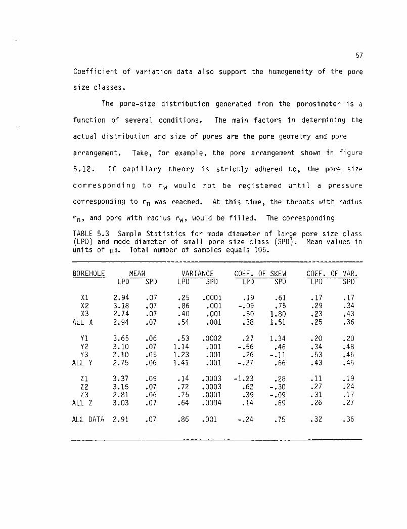
57

Coefficient of variation data also support the homogeneity of the pore

size classes.

The pore-size distribution generated from the porosimeter is a

function of several conditions. The main factors in determining the

actual distribution and size of pores are the pore geometry and pore

arrangement. Take, for example, the pore arrangement shown in figure

5.12. If capillary theory is strictly adhered to, the pore size

corresponding to r w would not be registered until a pressure

corresponding to rn was reached. At this time, the throats with radius

r n , and pore with radius rw , would be filled. The corresponding

TABLE 5.3 Sample Statistics for mode diameter of large pore size class(LPD) and mode diameter of small pore size class (SPD). Mean values inunits of 10. Total number of samples equals 105.

BOREHOLE MEANSPD

VARIANCE COEF. OF SKEW COEF.OF VAR.LPD LPD SPD LPD SPD LPD SPD

X1 2.94 .07 .25 .0001 .19 .61 .17 .17X2 3.18 .07 .86 .001 -.09 .75 .29 .34X3 2.74 .07 .40 .001 .50 1.80 .23 .43

ALL X 2.94 .07 .54 .001 .38 1.51 .25 .36

Y1 3.65 .06 .53 .0002 .27 1.34 .20 .20Y2 3.10 .07 1.14 .001 -.56 .46 .34 .48Y3 2.10 .05 1.23 .001 .26 -.11 .53 .46

ALL Y 2.75 .06 1.41 .001 -.27 .66 .43 .46

Z1 3.37 .09 .14 .0003 -1.23 .28 .11 .19Z2 3.15 .07 .72 .0003 .62 -.30 .27 .24Z3 2.81 .06 .75 .0001 .39 -.09 .31 .17

ALL Z 3.03 .07 .64 .0004 .14 .69 .26 .27

ALL DATA 2.91 .07 .86 .001 -.24 .75 .32 .36

Figure 5.12. Pore with wide radius, rw , and throats with narrowradius, rn.

58

59

0

0.2

OA 0.6

0.8

1.0

V/Vm

Figure 5.13. Initial intrusion/extrusion plot of pore diameter vs

cummulative intruded volume of Hg (cm 3/gm). Vm totalvolume intruded. V = cummulative intruded volume.

0 0.2 0.4 0.6

V/Vm0.8 1.0

102

EXTRUSION I10

INTRUSION ••

10-3

60

Figure 5.14. Second intrusion/extrusion plot of pore diametervs cumulative intruded volume of Hg (cm3/gm).Vm = total volume intruded. V = cumulativeintruded volume.

61

intrusion volume would apply to the smaller pore size, when actually a

portion of the intruded mercury volume should have been credited to the

larger pore size. This was termed volume hysteresis in Chapter Three.

This phenomenon probably occurs at every range of pressures over

the intrusion/extrusion cycle. The pore size distributions generated

are more of a cummulative distribution such that measured pore sizes not

less than a certain size are measured at each pressure increment. For

tnis reason the results here are tabulated as pore size classes and

modes of these classes instead of absolute pore-size distributions.

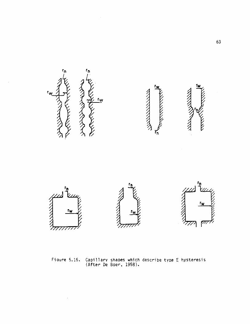
De Boer (1958) gave an explanation on shapes of capillaries by

studying the types of hysteresis loops generated from various pore

structures. Figures 5.13 and 5.14 show typical first run and second run

intrusion/extrusion curves from the non-welded tuff samples studied

here. Figure 5.15 shows five types of hysteresis loops as described by

de Boer. The type E hysteresis loop is characterized by a sloping

adsorption branch and steep desorption branch at intermediate pressures.

Capillary shapes which attribute to type E hysteresis are shown in

figure 5.16. Type E hysteresis can be compared to the first run

intrusion/extrusion cycle of figure 5.13. Although each sample displays

a certain amount of heterogeneity, it is hypothesized that capillary

structures with similar response to the ones pictured in figure 5.16

exist in the microstructure of the non-welded tuff samples.

The type A hysteresis loop compares favorably to the second run

curves of figure 5.14. De Boer describes type A loops as cylindrically

shaped capillaries which are open at both ends. Adhering to the local

hysteresis theory of Chapter three and the conclusion of Kloubek (1981),

62

V V

P/po

P/Po n4111. Pip 0

P/Po•nn1111. P/po

Figure 5.15. Fiva types of hysteresis loops describing differentPore arrangements (After De Boer, 1958).

63

InIn—,

/1-/–J laze z./ /

'Vr / r

rr,/ /

/////r/rr

Figure 5.16. Capillary shapes which describe type E hysteresis(After De Boer, 1958).

64

that mercury caps are being formed on already filled pores, suggests one

explanation for the different curve shape of the second run. The

comparison of the first run curve to the second run curve gives an

indication as to which pore sizes are trapping mercury. If the

intrusion/extrusion was completely reversible, one would expect the

curves to be identical, less machine variability and structural

degradation of the sample. Between 70 and 95% of the intruded mercury

is trapped inside the pores after the initial run. When comparing the

initial run to the second, from figures 5.13 and 5.14, it appears that

pores in the large to medium size range are trapping most of the

mercury. Perhaps this pore size class is most abundantly surrounded by

pores or throats of smaller radius.

TABLE 5.4 Summary statistics for pore surface area (PAREA) in m 2/gm andsurface area percentage attributable to(LPSAPER) in %.

the large pore size class

BOREHOLE MEAN VARIANCE COEF. OF SKEW COEF. OF VARPAREA LPSAPER PAREA LPSAPER PAREA LPSAPER PAREA LPSAPER

X1 3.18 2.50 .04 .31 1.74 1.04 .07 .22X2 3.29 3.37 .33 3.95 2.40 .16 .17 .59X3 3.05 3.13 .18 1.41 .80 -.23 .14 .38ALL X 3.16 3.09 .20 2.06 1.87 .46 .14 .46

Y1 3.07 3.27 .18 5.67 -.05 .90 .14 .73Y2 4.39 3.16 14.37 3.56 3.20 .28 .86 .60Y3 4.84 4.95 19.71 8.45 2.02 -.52 .91 .59ALL Y 4.33 4.00 13.83 6.67 2.66 .17 .86 .64

Z1 3.11 2.39 .46 2.86 .45 .92 .22 .71Z2 2.96 4.26 .25 4.24 .10 .58 .17 .48Z3 2.76 4.01 .15 2.97 -.59 .15 .14 .43ALL Z 2.90 3.77 .25 3.69 .39 .38 .17 .51

ALL DATA 3.47 3.72 5.06 4.49 4.83 .63 .65 .57

65

This phenomenon may only be a function of the type of slightly

welded tuff studied here. Further study into this area could lead to

quantification of mercury-trapping pore sizes. Further study into

actual pore geometries and arrangements could be advanced with the use

of scanning electron microscopy.

5.3 Pore Surface Area

The surface area of pores encountered in all samples was

calculated using equation 3.5. The work required to force mercury into

pore spaces is independent of any geometry assumption for pore structure

(Rootare and Prenzlow, 1967). Pore area statistics are given in table

5.4.

The pore surface area variation of all sample data is given in

figures 5.17 to 5.19. The pore surface area ranged from 1.96 m 2/gm in

sample UP (see figure 5.19) to 16.2 m 2/gm in sample JE (see figure

5.18). The mean pore area for all samples is 3.47 m 2/gm. In

comparison, according to Hillel (1980), a typical kaolinite clay mineral

has a specific surface of 5-20 m 2/gm. Rootare and Prenzlow (1967)

determined the surface area of 20 different powders using mercury

porosimetry and found good agreement with nitrogen adsorption. Calcium

cynamide, flourspar and fly ash all have surface areas comparable to the

Apache Leap Tuff.

A pocket of high porosity and high surface area is located near

the surface of boreholes Y2 and Y3. Gas trapped from the cooling ash

flow probably accumulated in this region causing larger porosities and

pore surface areas. Figure 5.20 presents a typical plot of pore size

and pore area distribution. Figure 5.20 combines the plots in figures

PORE SURFACE AREA (m 2/g)

0

MEAN(m )XI 3.18X2 3.29X3 3.05

-30

Figure 5.17. Pore surface area results from X borehole series.Borehole axes represent mean values. Plotted pointsrepresent difference from mean.

66

MEAN (rrt% )

Y I 3.08Y2 4.39Y3 4.84

PORE SURFACE AREA (m 2/g)

(r)

Fi aure 5.13. Pore surface area results from Y borehole series.Borehole axes represent mean val ues. Pl otted poi ntsrepresent di fference from mean.

67

PORE' SURFACE AREA (m2 /g)

Z3 Z2 Z I

MEAN (m1/9)Z I 3.11Z2 2.96Z3 2.76

-*--982°W 0

10-

30-

Figure 5.19. Pore surface area results from Z borehole series.Borehole axes represent mean values. Plotted pointsrepresent difference from mean.

68

69

5.1.a and 5.1.b. The bimodal pore size distribution is clearly apparent

as is the unimodal pore area distribution. As expected, the pore area

is skewed to the smaller pore sizes (positive skew). From table 5.4,

when considering all data, only 3.72% of the pore surface area is

accounted for by the large pore size class (upper modal distribution).

The pore surface area gives an indication of the potential wetted area

of rock at different fluid potentials. It is evident from the results

that a large negative potential must exist to thoroughly dry the

abundance of surface area contained in the tuff samples. The

limitations of the poresizer prevented study of pores sized below 6 nn

but it is expected that an even larger percentage of surface area

accounted for by the smaller pore size class exists.

The strongest linear correlation of any of the parameters studied

when considering all data exists between the porosity accounted for by

the large pore size class and the pore surface area accounted for by the

large pore size class. The correlation coefficient is 0.841 along with

a positive covariance of 26.5. This suggests that a higher than average

porosity percentage from the large pore size class is most likely paired

with a higher than average surface area percentage from the large pore

size class. In short, more large pores produce greater surface area

percentage from the large pores. A scattergram plot of porosity

percentage from the large pore size class (LPDPER) versus the surface

area percentage from the large pore size class (LPSAPER) is shown in

figure 5.21.

Generally, more surface area from the large pore size class

exists with depth along the boreholes. This is in agreement with the

100

90

80

70

LIJ 60

oa.

1• 50

p 40

30

20

I t

10

1%

°II i

tIt i i1 I 1• i1 I 1.—Pore Size1 I iI I

• II I I1 I II I II

1 4 1i1

,1Ii

1 ea' i•% a' i

so 0. 1

'Will SurfaceArea

% •.. •• ..,

,nnI•60.01 0.1 1 10

EQUIVALENT PORE DIAMETER (pm)

Figure 5.20. Plot of relative pore surface area and pore-sizedistribution vs pore diameter.

70

90

BO

70 o

o o;ea. ° D o

o o• x g

o 00 X

Xx x X

o

N o 4

oo

' o

60

0.

50 •X

NI 4 1140 r

• .30

20 r-

1 0 -

2 4 6 8 10 12

PORE SURFACE AREA PERCENTAGE FROM LARGE PORE SIZE CLASS (LPSAPER). Z

Figure 5.21. Scattergram plot of porosity percentage from large poresize class (LPDPER) vs pore surface area percentagefrom large pore size class (LPSAPER). X series datadenoted by 'x'; Y series by 'o'; Z series by '*'.

71

72

porosity percentage increasing with depth. All of this data can be

related to the moisture characteristic curve of the rock matrix. By

applying capillary theory to the data on pore size distribution and

using the surface area measurements, predictions as to the shape of the

curve can be generated.

Mercury porosimetry determinations of surface area and porosity

do not directly correspond to water availability estimates. Most of the

surface area here is accounted for by small pore sizes. During mercury

intrusion, mercury is forced into smaller and smaller pores. The

intrusion is only a function of the pressure applied because of the non-

wetting nature of mercury to most surfaces. Water, on the other hand,

is held in pores by capillary tension and also around matrix particles

by adhesion (see figure 5.22). A pore size distribution generated by

water desaturation accounts for total removal of water, both from

capillary wedges and from particle surfaces.

For this reason, the pore size distribution generated from

mercury porosimetry may underestimate the water availability at a

certain pressure/suction value. With a high percentage of surface area

avialable from small pores, water is most likely held in greater tension

but may benefit from less tortuosity in the small pore size domain.

Depending on the arrangement of large and small pores, the water

conducting properties of the tuff matrix could be enhanced (large pores

grouped together, small pores grouped together) or hindered (pores

interspersed creating a large tortuosity effect in transmission of

water).

Figure 5.22. Capillary wedge and adhesion of water on matrixparticle.

73

74

5.4 Spatial Variability

Recalling information presented in Chapter 3; the variogram is

the arithmetic mean of the squared differences between two experimental

measures Z(x) and Z(x+h) at any two points separated by the vector h.

Within a certain locality, the variability between these two points is

only dependent on the distance h and not on location x. A variogram (or

as used here, a semi-variogram), is a tool for analyzing the spatial

distribution of variables.

On average, the difference between two points or sample volumes

increases as the distance between them increases. The variogram can be

considered an estimation variance, that is, the variance of the error

committed when the value at a point x, is estimated by a value at point

(x+h). According to Journel and Huijbregts (1978) the quality of

estimation depends on four factors. They are:

1) The relative distances between what is to be estimated and the

information used to estimate it.

2) The size and geometry of what is to be estimated.

3) The quantity and spatial arrangement of the estimating

information.

4) The degree of continuity of the phenomenon under study, which is

conveyed by its characteristic semi-variogram.

Semi-variograms have been constructed for the seven parameters

studied here. The variability between points Z(x) and Z(x+h) is due to

several factors, each on a nested range of scales. The scales vary from

sampling errors (h-- 0), to the petrographic level (h < 1 cm) to the

stratification level (h=100 m) to the province level (h > 1 km). All of

75

these scales may be acting simultaneously at all levels of h, causing

data variability. It is often difficult to characterize even a single

structural scale. The micro-variabilities, those at a distance less

than the minimum sampling distance, are represented on the semi-

variogram by a discontinuity or "nugget" at the origin.

The semi-variograms generated are contained in figures 5.23-

5.29. All sample data (105 points) were used in construction of the

graphs. The three dimensional variogram program GAM3D (Geomath, 1987)

was utilized for this purpose. VPLOT2 (Geomath, 1987), a program

designed to plot both experimental and theoretical variograms, was used

to match theoretical data to experimental data. All variograms are

global in the sense that they are not directional. The class size

employed varied between 2.5 and 4 meters. None of the data sets were

transformed.

If the semi-variogram exhibits a sill value, which is the point

where the curve becomes more or less stable, the lag distance where it

occurs is called the range. The sill value is simply the a priori

variance of the random function Z(x). The range or zone of influence

defines the maximum distance at which the data are correlated.

Spherical variogram models were fit to the experimental data in

figures 5.23, 5.24 and 5.26 representing BULK, porosity and [PD,

respectively. The porosity value for sample SU of 47.58 was replaced by

the mean value of 14.8% when generating figure 5.24. It is obvious from

the data that an instrument malfunction or physical impairment of the

sample occurred during the porosimetry experiment because the porosity

percentage was greater than twice the maximum percentage obtained from

000o

1SPHERICAL 1

o CO =0.0008 AO =0.0 1o ! Ci =0.0037 A1 =9.0ô 18

I f 1 I 1 _____J5.8 11.7 17.5 29.3 29.2 85.0

(M)

DIRECTION = O. WINDOW = 90. MEAN = 2.130CLASS SIZE = 4.00

VARIANCE = 0.0043LOGARITHMS - NO

NO. OF SAMPLES = 105

Figure 5.23. Semi-variogram of bulk density results.

76

ooo

SPHERICALCO =1.400 AO =0.0C1 =3.000 A1 =6.0

ooo

0.0 5.8 /1.7 17.5 23.3

On)29.2 35.0

DIRECTION = O. WINDOW = 90. MEAN = 14.300CLASS SIZE = 4.00 VARIANCE = 4.2400LOGARITHMS - NO NO. OF SAMPLES = 105

Figure 5.24. Semi-yariogram of porosity results.

77

•MN,

oco

GAUSSIANCO =4.000 AO =0.0

oC1 =4.500 Al. =40.0

to

78

•

0.0 5.8 11.7 17.5 23.3(ht)

29.2 35.0

DIRECTION = O. WINDOW = SO. MEAN = 3.470CLASS SIZE = 4.00 VARIANCE = 5.0600LOGARITHMS - NO NO. OF SAMPLES = 105

Figure 5.25. Semi-variogram of pore surface area results. Dotted linerepresents pure nugget effect (random variogram—nocorrelation).

SPHERICALCO =0.200 AO =0.0Cl =0.680 Al =8.5

««

««

«

oon

+4

nNni

m4

CC gZ r..Z .

LI

nNM

0

Qooo I I I I I

0.0 5.8 11.7 17.5 23.3

29.2 35.0

(ht)

DIRECTION = O. WINDOW = SO. MEAN = 2.810CLASS SIZE = 4.00 VARIANCE = 0.8630LOGARITHMS - NO NO. OF SAMPLES = 105

Figure 5.26. Semi-variogram of mode diameter of large pore

size class results.

79

=0.0=40.0

o++Co

80

azEatz

C

rs.oo

GAUSSIANCO =0.0004C1 =0.0009

AOA1

C

o

ino

+

CC

o 4- +

+

i

5.8 11.7

moôo

Coooo

0.0 17.5

23.3

29.2 35.0

DIRECTION = O. WINDOW = SO. MEAN = 0.066CLASS SIZE = 2.50 VARIANCE = 0.0006LOGARITHMS - NO NO. OF SAMPLES = 105

Figure 5.27. Semi-variogram of mode diameter of small poresize class results.

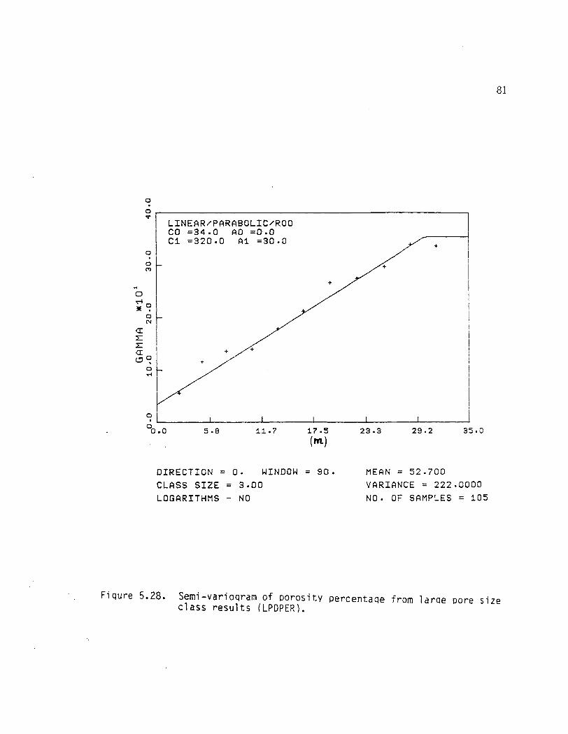
LINEAR/PARABOLIC/ROOCO =34.0 AO =0.0Cl =320.0 Al =30.0

81

5.8 11.717.5 23.3 29.2 35.0

o

o

DIRECTION = O. WINDOW = 90. MEAN = 52.700CLASS SIZE = 3.00 VARIANCE = 222.0000LOGARITHMS - NO NO. OF SAMPLES = 105

Figure 5.28. Semi-variogram of porosity percentage from large pore sizeclass results (LPDPER).

ooo0.4

LINEAR/PARABOLIC/ROOCO =0.900 AO =0.0

o Ci =8.000 Ai =38.00

oo• I

N

o

0.0 8.3 16.7 25.0 33.3 41.7 50.0( m )

DIRECTION = O. WINDOW = 90. MEAN = 3.710CLASS SIZE = 3.00 VARIANCE = 4.4800LOGARITHMS - NO NO. OF SAMPLES = 105

Figure 5.29. Semi-variogram of pore surface area percentagefrom large pore size class (LPSAPER).

82

83

any of the other samples. The nugget, range and sill of these three

semi-variograms are presented in table 5.5. These three parameters in

particular show very good structure of the study site deposit. The

local range of influence varies between 6 and 8.75 m. This is not the

range of influence for these parameters for the whole deposit but just

for the study site area. Kim (personal communication 1988) has shown a

range of influence for porosity structure in the horizontal direction

of several kilometers for similar material from the Ne-vada Test Site.

Notice the good agreement between the sample variance and the sill

values of the semi-variograms. Usually the sample variance is used as a

first approximation for the sill. In this case the variance is a "best"

approximation.

The nugget effect is very minimal for the bulk density values.

This suggests both a strong sampling procedure and minimal scale

effects. The higher nugget values for both porosity and LPD are

probably a function of the testing technique and the tuffaceous

material. Porosity variations of over 1% may well be accounted for by

core cutting and sample cutting from the cores. The porosity percentage

could certainly vary by 1.5% across the face of the 6 cm diameter core

TABLE 5.5 Semi-variogram results from figures 5.23, 5.24 and 5.26.

SAMPLE PARAMETER NUGGET RANGE (m) SILL VARIANCE

BULK .0008 8.75 .0045 .0043POROSITY 1.4 6.0 4.40 4.24LPD .2 8.2 .88 .86

84

because of the composition of the tuff. The nugget of 0.2 for the mode

diameter of the large pore size class is relatively small. The

histogram results are plotted on a logarithmic scale and a variation of

one bar width on the histogram results in a diameter difference of

greater than 0.2 for the upper pore size class.

Gaussian models were fit to the PAREA and SPD data sets shown in

figures 5.25 and 5.27. The effective range of a gaussian model is the

square root of 3 times its range (Geomath, 1987). The effective range

for each figure is approximately 11 meters. The nugget for pore area is

relatively high. The higher range and scale effect may play a

significant role in producing a high nugget for PAREA. A larger range

of sampling may reduce the appparent discontinuity at the origin. The

PAREA semi-variogram may also represent an absence of spatial

correlation or pure nugget effect represented by the dotted line on

figure 5.25. With this interpretation, spatial independence exists at

all scales presented and the best estimator at any point in the deposit

is the mean value. The SPD semi-variogram is subject to the same

restrictions as the LPD only to a higher degree because of the greater

relative difference in histogram bar widths.

Linear models best estimated the LPDPER and LPSAPER data in

figures 5.28 and 5.29. Linear models do not exhibit sill values so the

models were constructed with an estimated sill value. A close

inspection of these figures shows a fairly high degree of correlation

between the shapes of the two data sets. The correlation is supported

by the 0.841 correlation coefficient generated from the regression of

85

figure 5.21. High nugget values reflect the variability of the deposit

with respect to the bimodal distribution of pore size.

Overall, a definite structure exists in the tuffaceous deposit.

This data may be helpfull in determining sampling schemes for further

study into tuffaceous deposits being considered for high level nuclear

waste repositories.

5.5 Comparison With Other Methods

Porosity is related to bulk density and grain density by equation

5.1.

Porosity = 1 - (bulk density/grain density) (5.1)

Porosity and bulk density were determined on the Apache Leap Tuff core

by two different methods, mercury porosimetry and water saturation in

TABLE 5.6 Comparison of methods to determine bulk density, porosity,and grain density. M.P. = Mercury Porosimetry. SAT = Water Saturation.Sample size for M.P. = 2.5 cm diameter by 2.5 cm long. Sample size forSAT = 6 cm diameter by 5 cm long.

BULK DENSITY

EFFECTIVE POROSITY

GRAIN DENSITY(gm/cm 3 )

(%)

(gm/cm3 )

M.P. SAT M.P. SAT M.P. SAT

MAXIMUM 2.25 2.20 47.53 25.77 4.11 2.68MINIMUM 1.94 1.86 9.18 14.49 2.21 2.34MEAN 2.13 2.10 14.62 17.67 2.50 2.55MEDIAN 2.14 2.12 14.31 17.39 2.51 2.56COEF OF VAR .03 .03 .26 .12 .07 .02

86

the case of porosity and mercury porosimetry and physical measuring and

weighing in the case of bulk density. The data are found in Appendix B.

Figures 5.30 - 5.32 show bulk density variation along the boreholes.

Table 5.6 gives a synopsis of all data. Figure 4.1 shows a breakdown of

a typical 10 cm length of core and the lengths of each tested section.

In comparing the results from different methods, mercury

intrusion is in good agreement with the physically determined bulk

density values. Both methods have a coefficient of variation of 0.03.

When comparing mercury intrusion to water saturation to measure

porosity, the mean porosity is near 18% less than the value determined

from water saturation. This difference can be accounted for by the

maximum pressure applied during intrusion. Commercial porosimeters are

available which intrude mercury to a maximum pressure of 410 MPa.

Porosity determinations with these instruments would approach total

porosity. The variation in sample size between the two methods may also

account for some of the difference. Therefore, mercury intrusion is a

valid procedure in determining porosity as long as its limitations are

considered.

The difference in grain density is accounted for by the porosity

difference and equation 5.1. The maximum grain density of 4.11 gm/cm 3

from sample SN is not a true indication of grain density. A porosity

value of 47.58 generated from the intrusion results is in error, causing

the large grain density value. Evaluating the original data output

shows a porosimeter malfunction for this sample run.

BULK DENSITY(g/cm3 )XI X2

-.— S82°WX3

0

XI 2.15X2 2.11X3 2.14

Figure 5.30. Bulk density results from X series boreholes. Boreholeaxes represent mean values. Plotted points representdifference from mean.

87

BULK DENSITY (g/cm3 )

Y I ' Y2SE32° W Y3

MEAN (43/c.rn 3 )Y I 2.13Y2 2.14Y3 2.13

-30

88

0

Figure 5.31. Bulk density results from Y series boreholes.Borehole axes represent mean values. Plotteopoints represent difference from mean.

BULK DENSITY (g/cm3 )Z3 Z2 Z I

S82°W 0

10-

0 20-

30

MEAN(9/cm3)Z I 2.12Z2 2.10Z3 2.16

Figure 5.32. Bulk density results from Z series boreholes. Boreholeaxes represent mean values. ?lotted points representdifference from mean.

89

90

5.6 Comparison With General Trend of the Area

To get an indication of rock properties outside of the study site

location, 8 samples were obtained along the roadside of the Magma Mine

Road between US Highway 60 and the study site. Sample locations were

chosen at approximate 30 m elevation intervals. A modified chain saw

equipped with a 15 cm diamond coring bit 2.9 cm in diameter was used to

drill out each sample. In an attempt to minimize surface effects, the

outside 5 cm of core was cut off and discarded.

The roadside samples were gathered and analyzed for 2 reasons.

They are: 1) For a general comparison with the study site location; and

2) To act as an indicator for any blatent heterogeneity present in the

deposit. A statistical summary of results appears in table 5.7. All

sample means from the 8 roadside samples are within 2 standard

deviations of the study site means. A t-test (Miller and Freund, 1977)

was performed on the sample means for each of the variables from the

study site and the roadside. A significant difference occurred between

the two means for the variables PAREA and LPSAPER. When comparing the

TABLE 5.7 Summary statistics From Magma Mine Road samples. Number ofsamples = 8.

SAMPLE PARAMETER MEAN VARIANCE SKEW COEF OF VARIATION

BULK (gm/cm3 ) 2.15 .005 1.45 .03POROSITY (%) 14.98 7.54 -.49 .18PAREA (m2/gm) 2.521 .42 -.06 .26LPD (um) 2.64 .47 .41 .26SPD (um) .096 .004 1.92 .67LPDPER (%) 62.86 373 -.74 .31LPSAPER (%) 6.21 10.4 -.07 .52

91

coefficient of variation between the two data sets, only the SPD

variation is significantly higher than the study site sample data set.

The coefficient of variation is perhaps the only variable that can be

compared because of the drastic difference in the number of sample

points for each set.

Because of the minimal number of samples from the roadside data

set it is difficult to confidently present any data trends. All sample

parameters were regressed against each other and certain trends emerged.

Two trends or corrleations that were most important were those of pore

surface area, PAREA, versus the porosity percentage from the large pore

size class, LPDPER, and LPDPER versus the surface area percentage from

the large pore size class, LPSAPER. These two correlations showed the

strongest linearity, -.69 and .84, respectively, from the study site

samples. Data from the roadside samples produced correlation

coefficients of -.77 and .96 for PAREA versus LPDPER and LPDPER versus

LPSAPER, respectively. This analysis supports the homogeneity of the

tuffaceous deposit.

Samples were also obtained from 8 other locations near the study

site representing the gray zone (moderately welded) and the brown zone

(densely welded) of the Apache Leap Tuff (See figure 2.3). Gray zone

samples were drilled along the roadcut of US Highway 60 in Queen Creek

Canyon above the new highway tunnel on the north side of the road.

Brown zone samples were drilled out of the exposed bedrock just west of

the tunnel of old US Highway 60 (see figure 2.1). The coring device

mentioned above was used for this purpose.

92

A statistical summary is given in table 5.8. The upper pore size

class is absent from the data results obtained by mercury porosimetry

from the 2 lower tuffaceous units. This results in reduced porosity and

greater bulk density. Pore surface area is increased as more of the

porosity is accounted for by the pore sizes of less than 1 micrometer.

Porosities ranged from 5.4% to 8.7% for the moderately welded to densely

welded samples. The greater degree of compaction and degassing of the

deposit as it cooled played a major role in the decreased porosities.

TABLE 5.8 Summary statistics for brown (densely welded) and gray(moderately welded) zones of Apache Leap Tuff. Four samples per dataset. Upper set is from the gray, lower brown.

SAMPLE PARAMETER MEAN VARIANCE SKEW COEF OF VARIATION

BULK (gm/cm3 ) 2.45 .0004 -.02 .009POROSITY (%) 5.91 .171 -.78 .07PAREA (m2/gm) 3.31 .10 .17 .09SPD (%) .047 .0003 1.52 .34

BULK (gm/cm 3 ) 2.33 .0004 .53 .009POROSITY (%) 7.22 1.72 .16 .18PAREA (m2/gm) 6.60 2.19 .62 .22SPD (%) .024 .0002 .86 .58

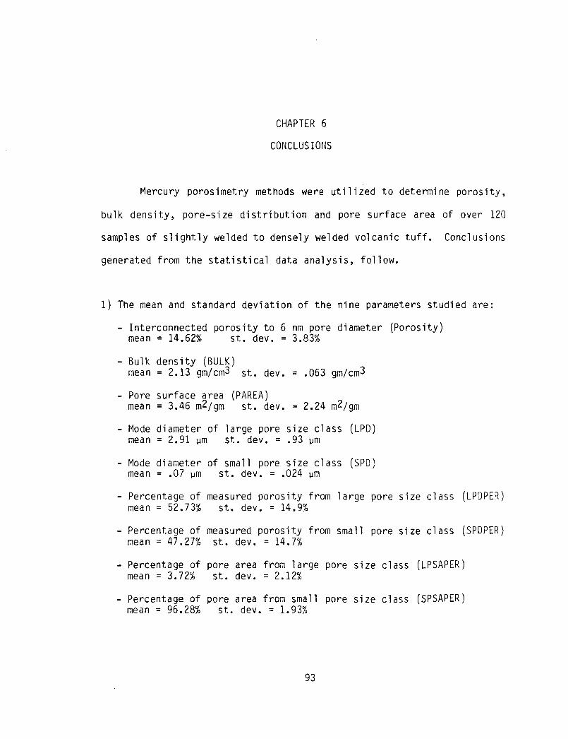
CHAPTER 6

CONCLUSIONS

Mercury porosimetry methods were utilized to determine porosity,

bulk density, pore-size distribution and pore surface area of over 120

samples of slightly welded to densely welded volcanic tuff. Conclusions

generated from the statistical data analysis, follow.

1) The mean and standard deviation of the nine parameters studied are:

- Interconnected porosity to 6 nm pore diameter (Porosity)mean = 14.62% st. dey. = 3.83%

- Bulk density (BULK)mean = 2.13 gm/cm3 st. dey. = .063 gm/cm 3

- Pore surface area (PAREA)mean = 3.46 m2 /gm st. dey. = 2.24 m2/gm

- Mode diameter of large pore size class (LPD)mean = 2.91 pm st. dey. = .93 pm

- Mode diameter of small pore size class (SPD)mean = .07 pm st. dey. = .024 pm

- Percentage of measured porosity from large pore size class (LPDPER)mean = 52.73% st. dey. = 14.9%

- Percentage of measured porosity from small pore size class (SPDPER)mean = 47.27% st. dey. = 14.7%

- Percentage of pore area from large pore size class (LPSAPER)mean = 3.72% st. dey. = 2.12%

- Percentage of pore area from small pore size class (SPSAPER)mean = 96.28% st. dey. = 1.93%

93

94

2) A bimodal pore-size distribution exists for samples of slightly

welded tuff of the Apache Leap study site. The distributions are

described in terms of the modes of the pore diameters from each pore

size class, upper (large) and lower (small).

3) Porosity results from mercury porosimetry are in relative terms 18%

lower than the saturation method compared here.

4) The lower pore size class accounted for most of the surface area of

the pores which averaged 3.47 m 2/gm. The range of percentage of surface

area accounted for by the lower pore size class varied from 89.91% to

99.93%.

5) Sample parameters of bulk density, porosity and mode diameter of the

upper pore size class showed the strongest structural trends in the

analysis of spatial variability. The local range of influence for these

3 parameters varied between 6 and 9 m. The range of influence in the

study site location for pore area is approximately 11 meters. The range

of influence here should not be confused with the range of influence of

the entire tuffaceous deposit which could be as high as several

kilometers.

6) Overall, more porosity was accounted for by the upper pore size class

as the distance from the land surface increased. A similar correlation

exists for the pore area percentage accounted for by the upper pore size

class.

7) The best linear correlation exhibited between two parameters was

found between the porosity percentage from the upper pore size class and

pore area percentage of the large pore size class. The correlation

coefficient was 0.841.

95

8) Samples of the moderately welded to densely welded tuff exhibited a

near log-normal distribution with respect to pore size with the mode

diameter averaging 0.035 pm.

9) Mercury porosimetry measurements in excess of 200 MPa applied

pressure are needed to fully determine porosity of the tuff samples.

Pore diameters less than 6 nm were not measured by the poresizer because

of instrument limitations. A significant percentage of total porosity

exists below the 6 nm range for the slightly to densely welded tuff

samples studied here. A quantitative measure of the percentage of total

porosity less than 6 nm is accounted for by the comparison of mercury

porosimetry results to water saturation results.

10) Porosimetry results agree strongly with physical measurement results

in terms of bulk density determinations.

11) Mercury porosimetry may underestimate the water content at high

suction values because of the adhesion layer effect of water on matrix

particles.

12) Mercury intrusion results compare more favorably to water

desaturation curves when considering the functional pressure

relationships of the matrix geometry. In short, large pores are

intruded with mercury before smaller pores. This compares directly with

larger pores emptying first when a suction is present in terms of water

desaturati on.

APPENDIX A

MERCURY INTRUSION PROCEDURES

Contained in this appendix is a complete step-by-step proceduralguide to mercury porosimetry as it applies to this study. Originalprocedures and guidelines were supplied by Micromeritics Corporation(1986).

96

DIRECTIONS FOR MERCURY INTRUSION

1. Make sure core sample is cut to proper specifications (26 min diam.

x 26 mm long maximum).

2. Oven dry samples until further weight loss is negligible. This is

usually a minimum of 48 hours.

3. Place oven dry samples into small aluminum containers, mark with id

number, and seal.

4. When ready for intrusion test, remove the sample from the aluminum

container, weigh it, and record the weight.

5. Using the proper penetrometer (see page 3-4 of manual) lightly

grease the ground joint of the penetrometer cap with Apiezon grease.

6. Place sample into penetrometer cup, cap it and seal with appropriate

spring assembly.

7. Reweigh sample and penetrometer assembly and record the weight.

8. Repeat steps 4 through 7 using a different penetrometer and sample

if analyzing two samples at once.

9. Install the penetrometers into the right and left preparation ports

on the front of the poresizer 9310. To do this, remove the capacitance

detector, turn the port counterclockwise to loosen, and remove the dummy

rod. Install the assembled penetrometer (lightly greased with vacuum

grease on the capillary end of the rod) and tighten the port.

97

98

10. Make sure either a. dummy rod or penetrometer fills both ports

before evacuating the system.

11. At this point load the poresizer program into the IBM PC. Put the

Micromeritics Program disc into drive A and the Data disc in drive B. It

will respond with a prompt to turn on the poresizer. Do this by

engaging the switch on the front of the poresizer. A prompt will appear

asking if a pen plotter will be used. Respond with a carriage return

(CR). The menu table will now appear on the screen.

12. Press the "EVACUATE SLOW" button and the "LOW PSIA" button on the

front of the poresizer. Note the atmospheric pressure reading on the

poresizer. Turn on the vacuum pump. When the pressure drops below 0.5

psia, push the "um Hg" button and the "FAST EVACUATE SAMPLE" button.

13. The pressure should drop rather rapidly to between 500 and 700

microns. To test for leaks in the evacuation system, depress the

"EVACUATE SAMPLE" buttons and watch the pressure reading. If it

increases rapidly there is a leak in the system. The leak is probably

around the penetrometer stem where it seats into the preparation port.

Move the penetrometer back and forth and see if the leak subsides. (the

penetrometer should not move more than 1 cm in and out.) Press the "FAST

EVACUATE SAMPLE" button again and see if the pressure starts decreasing.

The optimal vacuum is near 50 pm.

14. When the "best" vacuum is reached, press the "MERCURY FILL" switch.

You have to manually hold the switch in for mercury to fill into the

penetrometers. Hold the "MERCURY FILL" switch in until the red "UP"

light comes on.

99

15. Release the fill button. Release the "FAST EVACUATE SAMPLE"

button. Shift the pressure reading back to low psia by pressing the

"LOW PRESSURE PSIA" button.

16. Momentarily press the "ADJUST LOW PRESSURE" button until the

pressure is between 0.5 and 1.5 psia.

17. IMPORTANT: Press the "EVACUATE RESERVOIR" button. The pump will

return to its normal operating sound in 20 to 30 seconds. This step is

important because the mercury needs to be released from the "up"

position. It is paramount that the reservoir is at the same potential

as the rest of the system or a mercury leak could occur. DO NOT RELEASE

THE "EVACUATE RESERVOIR" BUTTON.

18. Hold the "MERCURY DRAIN" button in until the green "down" indicator

illuminates on the front panel. Release the "MERCURY DRAIN" button. Now

release the "EVACUATE RESERVOIR" button. You can shut off the vacuum

pump at this stage.

19. Depress the "ADJUST LOW PRESSURE" button until the pressure reaches

atmospheric.

20. The low pressure/sample preparation run is now complete. Remove

the penetrometers and reweigh them.

NOTE

While the vacuum pump is evacuating the sample(s) you can be entering

data for the run. Below is a listing of what you will see appear on the

screen. Follow the step by step procedure as given in the example

below.

LISTINGS FROM MICROMERITICS PROGRAM

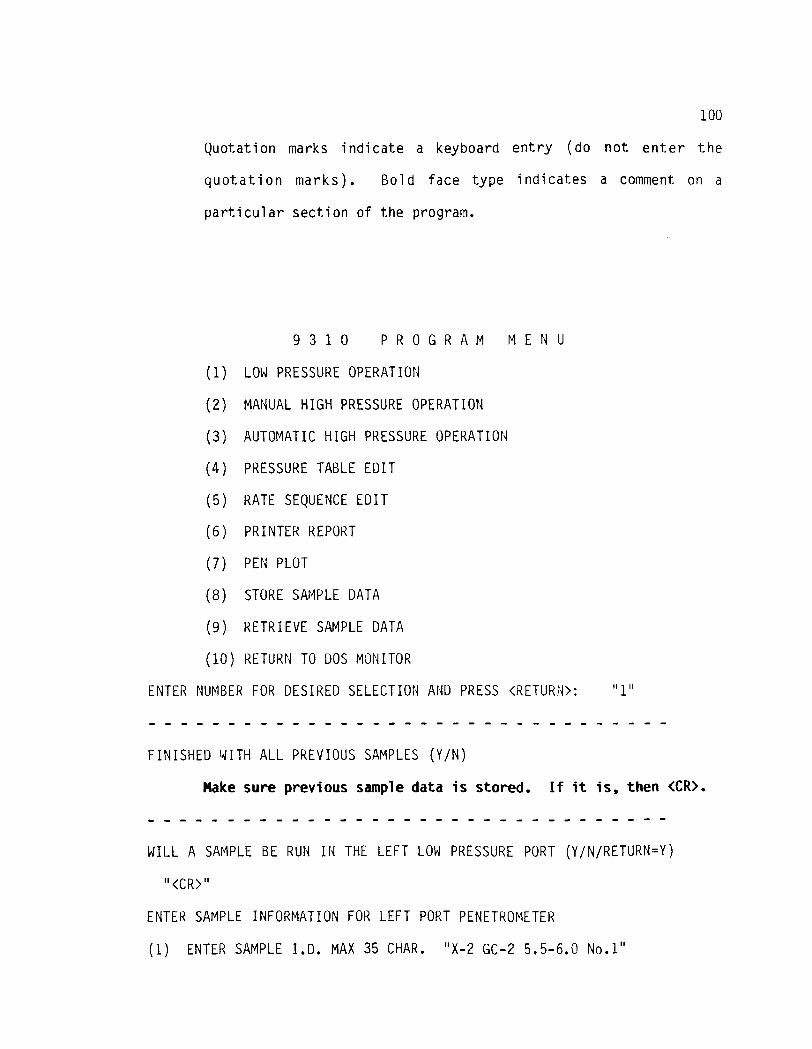
100

Quotation marks indicate a keyboard entry (do not enter the

quotation marks). Bold face type indicates a comment on a

particular section of the program.

9310 PROGRAM MENU

(1) LOW PRESSURE OPERATION

(2) MANUAL HIGH PRESSURE OPERATION

(3) AUTOMATIC HIGH PRESSURE OPERATION

(4) PRESSURE TABLE EDIT

(5) RATE SEQUENCE EDIT

(6) PRINTER REPORT

(7) PEN PLOT

(8) STORE SAMPLE DATA

(9) RETRIEVE SAMPLE DATA

(10)RETURN TO DOS MONITOR

ENTER NUMBER FOR DESIRED SELECTION AND PRESS <RETURN>: "1"

FINISHED WITH ALL PREVIOUS SAMPLES (YIN)

Make sure previous sample data is stored. If it is, then <CR>.

WILL A SAMPLE BE RUN IN THE LEFT LOW PRESSURE PORT (Y/N/RETURN=Y)

"<CR>"

ENTER SAMPLE INFORMATION FOR LEFT PORT PENETROMETER

(1) ENTER SAMPLE I.D. MAX 35 CHAR. "X-2 GC-2 5.5-6.0 No.1"

101

(2) ENTER SUBMITTED I.D. MAX 35 CHAR. "GTV"

(3) ENTER DATE OF ANALYSIS MAX 10 CHAR. "AUG 1 87"

(4) ENTER TIME OF ANALYSIS MAX 10 CHAR. "1200"

(5) ENTER PENETROMETER NO. 11 4"

(6) ENTER PENETROMETER CONST. (uL/pF) DEFAULT=10.79 "33.13"

(7) ENTER PEN VOL. (cc) DEFAULT=5.0 "18.226"

(8) ENTER PEN STEM VOL. (cc) DEFAULT=0.412 "3.226"

(9) ENTER HEAD CORRECTION FACTOR DEFAULT=4.68 11 4.45"

(10)ENTER SAMPLE WEIGHT (g) DEFAULT=1.0 "25.67"

(11)ENTER SAMPLE+PEN WEIGHT (g) DEFAULT=2.0 "97.76"

(12)ENTER CONTACT ANGLE (degrees) DEFAULT=130 "<CR>"

(13)ENTER SURFACE TENSION (dynes/cm) DEFAULT=485 "<CR>"

(14)ENTER Hg DENSITY (g/cc) DEFAULT=13.5335 "<CR>"

(15)REPORT IN RADIUS OR DIAMETER (RID) DEFAULT=D "<CR>"

(1) SAMPLE I.D. =X-2 GC-2 5.5-6.0 No.1

(2) SUBMITTER I.D. =GTV

(3) DATE =AUG 1 87

(4) TIME =1200

(5) PEN. NO. =4

(6) PEN. CONST. =33.13

(7) PEN. VOL. =18.226

(8) PEN. STEM VOL. =3.226

(9) HEAD CORR. FACTOR =4.45

(10)SAMPLE WEIGHT =25.67

(11) SAMPLE+PENETROMETER WEIGHT =97.76

102

(12)CONTACT ANGLE =130

(13)SURFACE TENSION = 485

(14)Hg DENSITY =13.5335

(15)REPORT IN DIAMETER

ALL OK (Y/N/RETURN=Y) If yes, then <CR>

DO YOU WANT A PRINTER REPORT TO BE AUTOMATICALLY PRINTED AFTER THE HIGH

PRESSURE RUN IS COMPLETED (YIN) "N"

WILL A SAMPLE BE RUN IN THE RIGHT LOW PRESSURE PORT (Y/N/RETURN=Y) "N"

INSTRUCTIONS FOR LOW PRESSURE RUN

1. INSTALL ASSEMBLED PENETROMETER(S) AND/OR DUMMY ROD(S) IN BOTH PORTS.

2. DEPRESS EVACUATE SAMPLE SLOW AND LOW PSIA PRESSURE TRANSDUCER

BUTTONS.

3. TURN ON POWER SWITCH FOR VACUUM PUMP.

4. WHEN PRESSURE DROPS TO 1 PSIA (SEE MANUAL IF RUNNING A POWDER),

RELEASE EVACUATE SAMPLE SLOW BUTTON AND DEPRESS EVACUATE SAMPLE MED and

um PRESSURE TRANSDUCER BUTTONS.

5. BEWARE OF SAMPLE FLUIDIZATION.

6. WHEN PRESSURE DROPS TO 250 um, RELEASE MED EVACUATE SAMPLE BUTTON

AND DEPRESS FAST EVACUATE BUTTON.

7. INSTALL CAPACITANCE DETECTORS OVER PENETROMETER ASSEMBLIES.

8. WHEN PRESSURE DROPS TO 50 um (OR HAS EQUILIBRATED AT SOME LOWER

PRESSURE), DEPRESS Hg FILL BUTTON MOMENTARILY. IF LOSS OF

VACUUM, ALLOW LONGER EVACUATION, OTHERWISE HOLD UNTIL Hg UP LIGHT IS ON.

IF LIGHT GOES OUT, DEPRESS Hg FILL BUTTON UNTIL LIGHT COMES ON AGAIN.

103

9. PRESS 'SPACE-BAR' TO CONTINUE.

10.TURN OFF EVACUATE FAST SAMPLE BUTTON AND CHANGE FROM um TO LOW PSIA

PRESSURE TRANSDUCER.

11. MOMENTARILY PRESS ADJUST LOW PRESSURE BUTTON UNTIL PRESSURE IS

BETWEEN 0.5 AND 1.5 PSIA.

12. DEPRESS EVACUATE RESERVOIR BUTTON AND WAIT 20 TO 30 SECONDS OR

UNTIL SOUND FROM VACUUM PUMP RETURNS TO NORMAL. DO NOT RELEASE THE

EVACUATE RESERVOIR BUTTON.

13. PRESS 'SPACE-BAR' TO CONTINUE.

TAKE BASE LOW PRESSURE AND INTRUSION READINGS AS FOLLOWS:

1. DEPRESS MERCURY DRAIN BUTTON UNTIL MERCURY DOWN LIGHT COMES ON.

2. RELEASE EVACUATE RESERVOIR BUTTON AND MERCURY DRAIN BUTTON.

3. TO TAKE BASE LOW PRESSURE AND CAPACITANCE READINGS, PRESS 'SPACE-

BAR'.

4. IF THE DATA IS OK, PRESS 'RETURN'.

5. LEFT PENETROMETER LOCATION BUTTON AND RIGHT PENETROMETER LOCATION

BUTTON ARE IGNORED AND CAN BE IN ANY POSITION.

WAIT APPROXIMATELY 10 SECONDS FOR READINGS

LOW PRESSURE =13.1 PSI

LEFT CAPACITANCE = 112.34 pF

RIGHT CAPACITANCE = 111.87 pF

ALL OK (Y/N/RETURN=Y/SPACE=ANOTHER BASE READING) "<CR>"

POINT NO. PRESSURE (PSIA) LEFT CAPACITANCE (pF) RIGHT CAPACITANCE (pF)

1 13 112.34 111.87

104

'SPACE-BAR' = TAKE ANOTHER READING 'F9' = STOP DATA COLLECTION

"Press F9"

1. RETURN THE SYSTEM TO ATMOSPHERIC PRESSURE BY LIGHTLY TAPPING THE

SLOW EVACUATION BUTTON UNTIL A PRESSURE BETWEEN 13.5 - 14.0 PSIA IS

REACHED.

2. THE LOW PRESSURE RUN IS NOW COMPLETE. REMOVE THE PENETROMETER(S)

AND REWEIGH IT (THEM).

3. PRESS 'SPACE-BAR' TO CONTINUE

ENTER LEFT PEN+SAM+Hg WEIGHT (g) DEFAULT=3.0 "165.78"

LEFT PEN+SAM+Hg WEIGHT = 165.78 G

ALL OK (Y/N/kETURN=Y) "<CR>" if all is OK

HIGH PRESSURE RUN

IMPORTANT

Before running the high pressure test make sure the hydraulic ram in the

high pressure chamber is at its lowest limit. You can check this by

pressing the scan down switch near the lower left corner of the

poresizer. Press the switch to down and wait for the motor to stop

running. Now bring the switch back to the neutral position. Now start

the high pressure run.

The following is a step-by-step review of the high pressure run program.

9310 PROGRAM MENU

(1) LOW PRESSURE OPERATION

(2) MANUAL HIGH PRESSURE OPERATION

105

(3) AUTOMATIC HIGH PRESSURE OPERATION

(4) PRESSURE TABLE EDIT

(5) RATE SEQUENCE EDIT

(6) PRINTER REPORT

(7) PEN PLOT

(8) STORE SAMPLE DATA

(9) RETRIEVE SAMPLE DATA

(10)RETURN TO DOS MONITOR

ENTER NUMBER FOR DESIRED SELECTION AND PRESS <RETURN>:

PREPARING TO RUN LEFT PENETROMETER IN HIGH PRESSURE SYSTEM

ENTER NUMBER OF PRESSURE TABLE TO BE USED (1-9/DEFAULT=1): "2"

PRESS F9 TO TERMINATE

DO YOU WISH TO EQUILIBRATE AT PRESSURE POINTS (Y/N/RETURN=Y): "Y"

ENTER EQUILIBRATION TIME (SEC) DEFAULT=10:

PRESS 'F9' TO TERMINATE "<CR>"

ADJUST 'SET ATM PRESSURE' ON 9310 UNTIL THE DISPLAY SHOWS 13-14 PSIA FOR

THE HIGH PRESSURE TRANSDUCER WITH THE HIGH PRESSURE CHAMBER VENTED TO

ATMOSPHERIC PRESSURE. THEN PRESS 'RETURN' TO RECORD OFFSET OR 'F9' TO

TERMINATE:

WAIT APPROX 10 SECONDS

106

CLOSE VENT VALVE AND PRESS 'RETURN' TO START HIGH PRESSURE RUN, 'F9' TO

TERMINATE RUN:

When the high pressure run is complete, store the data as

follows:

9310 PROGRAM MENU

(1) LOW PRESSURE OPERATION

(2) MANUAL HIGH PRESSURE OPERATION

(3) AUTOMATIC HIGH PRESSURE OPERATION

(4) PRESSURE TABLE EDIT

(5) RATE SEQUENCE EDIT

(6) PRINTER REPORT

(7) PEN PLOT

(8) STORE SAMPLE DATA

(9) RETRIEVE SAMPLE DATA

(10)RETURN TO DOS MONITOR

ENTER NUMBER FOR DESIRED SELECTION AND PRESS <RETURN>: "8"

SECOND HIGH PRESSURE RUN

Run two high pressure tests per sample. Upon completion of the

initial high pressure run and sample data storage, the main menu will

again appear. In order to start the second high pressure run go through

the same computer procedure as for the first run, i.e. enter the sample

data for the low pressure operation, etc.

107

The only change in the sample data will be in the sample id-where

this will be run No.2 and in the sample time. Enter the identical

values from the first run.

When it comes time to set atmospheric pressure before the high

pressure run, remember two things: (1) run the hydraulic ram motor

down by manually pressing the "SCAN DOWN" button, and (2) open the vent

valve on the top of the high pressure chamber.

Go through the same procedure after the second high pressure run

as after the first high pressure run, i.e. store the sample data, etc.

It is now time for clean-up. Open the vent valve on the high

pressure chamber to expose the system to atmospheric pressure. Unscrew

the high pressure chamber and let the oil drip from the penetrometer for

a few minutes.

SAFETY

Put on the safety goggles, rubber gloves, and surgeon's mask. Set

the used mercury container on the platform of the poresizer and put the

funnel into the container. Remove the penetrometer from the high

pressure chamber and hold over the funnel with stem down into funnel

tube. Carefully remove the penetrometer assembly by unlatching the

spring and removing. Set this aside on a paper towel along with the

black cap of the assembly. Next, while holding the penetrometer cup

inside the funnel, gently slide the stainless steel cap off the

penetrometer cup. Most of the mercury should drain out of the capillary

into the container. Now lift the penetrometer out of the funnel and put

a finger over the capillary and invert the cup over the funnel, dumping

108

the sample and remaining mercury into the funnel. Tap the penetrometer

cup on the side of the funnel to dislodge any remaining mercury and then

set aside on a paper towel.

It is important to remember to properly discard any contaminated

towelling, gloves, etc. in special receptacles for the hazardous waste

division to pickup. The intruded core samples should be treated the

same way.

TROUBLE SHOOTING

The poresizer manual is fairly thorough in diagnosing procedural

problems but does not detail diagnosing equipment problems.

1. The biggest problem most likely encountered will be with the vacuum

system. Do the best possible job to get the system to at least 300

micrometers Hg.

2. Faulty intrusion values.

If the poresizer registers intrusion values that either stay constant or

increase as pressure increases there is undoubtedly a problem with the

gold plated banana plug in the high pressure system. To rectify this

problem, drain the high pressure system of high pressure fluid. This is

accomplished with the use of a syringe. When all of the fluid is

removed take the long handled needle-nosed pliers and gently unscrew the

plug. Clean the plug and reinsert into the high pressure chamber. Do

not turn the plug too tight. When resistance is felt on the pliers you

have turned enough. Refill the chamber with fresh high pressure fluid.

If other problems occur consult the manual. Be safe with the

machine and it will be safe with you.

APPENDIX B

RAW SAMPLE DATA AND STATISTICAL TABLES

This appendix contains all raw data generated from the mercuryporosimetry study as well as data from physical measurement techniquesfor determining bulk density and water saturation techniques fordetermining porosity. Statistical tables are presented containingcorrelation coefficients for each individual borehole, each borehole setand for all borehole data.

109

110

Table Bi: Preliminary summary of physical properties obtained from coresegments at the Apache Leap Tuff Site. Columns labeled (med.)are results for medium core segments (2.5 cm diameter by 2.5cm length) from mercury porosimetry. Columns labeled (large)are results for large core segments (6 cm diameter by 5 cmlength) from water saturation method.

Bulk EffectiveDensity Porosity(g/cm3) (%)

med. large med. largeX Boreholes:

GrainDensity(g/cm3)

med. large

Maximum 2.25 2.19 17.94 21.10 2.59 2.60Minimum 1.94 1.97 9.80 14.30 2.21 2.34Mean 2.13 2.10 14.06 17.58 2.48 2.55Median 2.15 2.12 14.19 17.39 2.51 2.56Coefficient of variation 0.03 0.03 0.13 0.10 0.04 0.02

Y Boreholes:

Maximum 2.25 2.20 21.20 23.40 2.72 2.64Minimum 1.94 1.90 11.22 14.49 2.28 2.51Mean 2.13 2.10 15.04 17.72 2.51 2.56Median 2.14 2.12 14.90 17.44 2.53 2.56Coefficient of variation 0.03 0.03 0.14 0.12 0.03 0.01

Z Boreholes:

Maximum 2.25 2.19 47.58 25.77 4.11 2.68Minimum 1.95 1.86 9.18 14.77 2.22 2.37Mean 2.13 2.10 14.75 17.72 2.52 2.55Median 2.14 2.11 13.95 15.80 2.50 2.54Coefficient of variation 0.03 0.03 0.40 0.15 0.11 0.02

All Boreholes:

Maximum 2.25 2.20 47.58 25.77 4.11 2.68

Minimum 1.94 1.86 9.18 14.49 2.21 2.34

Mean 2.13 2.10 14.62 17.67 2.50 2.55

Median 2.14 2.12 14.31 17.39 2.51 2.56

Coefficient of variation 0.03 0.03 0.26 0.12 0.07 0.02

111

Table B2: Physical properties obtained from core segments at the ApacheLeap Tuff Site. Columns labeled (med.) are results for mediumcore segments (2.5 cm diameter by 2.5 cm length) from mercuryporosimetry. Columns labeled (large) are results for largecore segments (6 cm diameter by 5 cm length) from water

Borehole

saturation method. Results are preliminary.

Sample Depth Bulk EffectiveID (m) Density Porosity

(g/cm3) (%)

med. large med. large

GrainDensity(g/cm3)

med. large

X1 AA 2.10 2.11 2.11 10.91 17.36 2.37 2.55AB 2.90 2.13 2.13 11.84 16.23 2.42 2.55AC 3.80 2.15 2.13 13.50 17.40 2.48 2.58AD 6.90 2.18 2.12 12.40 16.48 2.49 2.54AE 10.00 2.18 1.99 12.80 14.99 2.50 2.34AF 12.70 2.16 2.18 15.10 16.11 2.54 2.60AG 15.80 2.16 2.18 14.10 15.98 2.52 2.60

X2 CA 1.90 2.08 1.97 14.20 21.10 2.43 2.50CB 2.90 2.04 2.06 9.80 18.76 2.26 2.54CC 3.60 2.04 2.04 10.50 18.80 2.27 2.51CD 6.60 2.14 2.12 13.50 2.47CE 10.00 2.11 2.13 15.85 17.39 2.51 2.57CF 12.70 2.13 2.00 15.31 17.87 2.51 2.44CG 16.10 2.00 2.06 17.94 18.33 2.44 2.52CH 18.50 2.18 2.06 14.88 19.21 2.56 2.55CJ 21.70 2.17 2.15 14.19 16.89 2.53 2.59CK 24.70 2.15 2.06 16.13 20.44 2.56 2.59CM 27.90 2.10 2.09 16.33 18.98 2.51 2.58CN 30.80 2.15 2.09 15.91 19.46 2.55 2.59

X3 EA 1.80 1.94 2.04 12.20 20.61 2.21 2.57EB 2.70 2.01 1.97 14.36 20.15 2.34 2.47EC 3.80 2.07 2.00 15.40 2.45ED 6.80 2.13 2.10 12.80 2.44EE 9.90 2.15 2.16 13.20 2.47EF 12.90 2.19 2.15 13.09 2.51EG 15.80 2.23 2.14 13.23 15.68 2.57 2.54EH 18.80 2.16 2.19 14.31 14.30 2.53 2.56Ed 21.70 2.20 2.15 12.55 15.27 2.51 2.54EK 24.70 2.19 2.17 14.02 15.96 2.55 2.58EM 27.70 2.25 2.16 12.27 16.22 2.56 2.58EN 31.00 2.11 2.07 16.34 17.17 2.52 2.50EP 33.60 2.10 2.12 17.47 17.18 2.54 2.56ER 36.90 2.19 2.12 15.38 17.42 2.59 2.56ES 39.90 2.15 2.11 14.91 18.31 2.53 2.58ET 42.90 2.11 2.12 15.39 17.42 2.50 2.57

112

Table B2 (Continued)

Borehole SampleID

Depth(m)

BulkDensity(g/cm3)

med. large

EffectivePorosity

(%)

med. large

GrainDensity(g/cm3)

med. large

Y1 GB 1.90 2.12 2.17 13.70 16.71 2.46 2.60GC 3.30 2.15 2.14 11.90 16.62 2.44 2.56GD 4.10 2.14 2.13 13.33 16.69 2.47 2.56GA 6.70 2.10 2.13 13.93 17.05 2.43 2.56GE 9.90 2.11 2.09 16.61 18.82 2.53 2.57GG 12.20 2.13 2.13 15.99 15.96 2.54 2.53GH 15.70 2.17 2.17 11.22 15.65 2.45 2.57

Y2 JB 1.90 2.02 2.01 16.65 23.40 2.43 2.63JC 3.30 2.25 2.04 12.20 19.16 2.56 2.52JD 4.10 2.21 2.08 13.30 18.61 2.55 2.55JE 6.20 2.12 2.08 19.00 16.87 2.62 2.51JF 9.30 2.10 2.13 12.83 17.21 2.41 2.58JG 12.30 2.13 2.04 14.95 20.64 2.50 2.58JH 15.30 2.11 2.11 15.94 18.09 2.51 2.57JJ 18.50 2.17 2.00 13.76 20.82 2.52 2.53JK 21.40 2.14 2.11 16.03 16.81 2.54 2.54JM 24.50 2.07 2.08 17.37 17.48 2.50 2.52JN 27.30 2.15 2.09 16.60 17.44 2.57 2.53JP 30.30 2.19 2.12 12.38 18.67 2.50 2.61

Y3 MB 2.00 1.99 2.02 14.40 20.36 2.32 2.53MC 3.10 1.94 2.03 14.90 2.28MD 4.10 2.15 2.05 21.20 22.43 2.72 2.64ME 6.20 2.15 2.01 14.64 2.52MF 9.40 2.15 2.17 16.42 2.57MG 12.40 2.02 1.90 17.37 2.44MH 16.00 2.11 2.10 14.64 17.79 2.47 2.55Md 18.20 2.23 2.18 12.63 14.55 2.55 2.55MK 21.30 2.25 2.20 11.96 14.49 2.55 2.57MM 24.20 2.23 2.15 13.68 14.70 2.59 2.52MN 27.40 2.20 2.15 14.85 16.15 2.58 2.56MP 30.30 2.16 2.14 15.50 17.56 2.56 2.59MR 33.30 2.19 2.17 15.70 16.48 2.59 2.59MS 36.50 2.10 2.12 17.21 18.18 2.54 2.59MT 39.30 2.09 2.13 18.10 17.11 2.55 2.57MU 42.20 2.15 2.15 15.61 16.94 2.55 2.59

113

Table B2 (Continued)

Borehole SampleID

Depth(m)

BulkDensity(g/cm3)

med. large

EffectivePorosity

(%)

med. large

GrainDensity(g/cm3)

med. large

Z1 PB 1.80 2.15 1.94 12.80 18.16 2.47 2.37PC 3.00 2.07 1.96 13.30 2.39PD 4.10 2.05 2.07 15.70 22.56 2.44 2.68PE 6.00 2.10 2.11 11.61 2.37PF 9.20 2.19 2.16 11.50 2.48PG 12.50 2.13 2.09 11.68 2.41PH 15.20 2.12 2.12 14.75 2.49

Z2 SB 2.00 2.18 2.14 13.80 17.43 2.53 2.60SC 3.00 2.20 2.18 12.50 16.58 2.51 2.61SD 3.90 2.08 2.11 12.70 16.87 2.38 2.54SE 6.50 2.13 2.11 14.51 16.93 2.50 2.54SF 9.40 2.06 2.03 16.92 20.84 2.47 2.56SG 12.50 1.95 1.86 12.27 25.77 2.22 2.51SH 15.30 2.03 2.08 14.12 17.44 2.36 2.51SJ 18.60 2.10 2.13 13.95 2.44SK 21.10 2.10 2.15 12.81 2.41SM 24.50 2.17 2.17 13.34 14.77 2.50 2.54SN 27.40 2.15 2.15 47.58 4.11SP 30.50 2.08 2.06 18.47 2.55

Z3 UW 2.00 2.23 2.17 12.50 15.80 2.55 2.58UC 3.00 2.16 2.12 14.08 16.80 2.51 2.55UD 3.80 2.14 2.05 15.07 18.80 2.52 2.53UE 6.70 2.10 2.10 9.18 17.41 2.31 2.54UF 9.70 2.08 2.11 14.53 16.38 2.44 2.52UG 12.70 2.17 2.06 15.18 19.41 2.56 2.56UH 15.90 2.06 2.00 11.77 19.41 2.33 2.48UJ 18.80 2.19 2.16 13.12 14.98 2.52 2.54UK 21.70 2.25 2.18 12.13 14.94 2.56 2.57UM 24.70 2.18 2.16 14.83 15.71 2.56 2.57UN 27.70 2.23 2.19 15.19 15.31 2.63 2.59UP 30.70 2.22 2.18 11.16 2.50UR 33.70 2.19 2.14 15.50 17.45 2.59 2.59US 36.80 2.13 2.11 16.65 2.56UT 39.80 2.14 2.11 16.99 2.58UU 42.80 2.19 2.12 14.32 2.56

114

Table B3: Summary of pore area and pore size distribution properties atthe Apache Leap Tuff Site. Columns labeled (upper) and(lower) refer to upper and lower peaks of the bimodal poresize distribution.

TotalPore Area

(m2/g)

X Boreholes:

Mode PoreDiameter

- - (um) - -upper lower

RelativePorosity

- - (%) - -

upper lower

RelativeArea

- - (%) --upper lower

Maximum 4.939 4.59 0.1470 67.38 74.09 6.88 99.64Minimum 2.207 1.72 0.0336 25.91 32.62 0.36 93.12Mean 3.162 2.94 0.0674 50.91 49.09 3.09 96.91Median 3.128 2.81 0.0702 54.30 45.96 3.17 97.09Coef. Var. 0.141 0.25 0.3438 0.21 0.22 0.46 0.01

Y Boreholes:

Maximum 16.510 4.59 0.1470 75.07 98.05 10.09 99.93Minimum 2.054 0.09 0.0098 1.95 24.93 0.07 89.91Mean 4.335 2.75 0.0609 52.00 48.00 4.29 95.71Median 3.221 2.81 0.0549 60.47 42.53 4.57 6.20Coef. Var. 0.845 0.43 0.4497 0.37 0.40 0.62 0.03

Z Boreholes:

Maximum 4.015 4.59 0.1150 89.17 70.20 8.52 99.15Minimum 1.960 1.72 0.0429 29.80 10.83 0.85 91.48Mean 2.900 3.03 0.0701 55.30 44.70 3.77 96.23Median 2.916 2.81 0.0702 55.44 24.80 3.74 96.44Coef. Var. 0.169 0.26 0.2628 0.23 0.28 0.50 0.02

All Boreholes:

Maximum 16.510 4.59 0.1470 89.17 98.05 10.09 99.93Minimum 1.960 0.09 0.0098 1.95 10.83 0.07 89.91Mean 3.466 2.91 0.0661 52.73 47.27 3.72 96.28Median 2.999 2.81 0.0549 55.04 44.56 3.50 96.45Coef. Var. 0.646 0.32 0.3568 0.28 0.31 0.57 0.02

115

Table B4: Pore area and pore size distribution properties at the ApacheLeap Tuff Site. Columns labeled (up) and (low) refer toupper and lower peaks of the bimodal pore size distribution.

Bore-hole ID

Depth(m)

TotalPore Area(m2/g)

Mode PoreDiameter

- - (um) - -

up low

RelativePorosity

- (%)-up low

RelativeArea

- (%) -up low

X1 AA 2.10 3.008 2.81 0.0702 36.56 63.44 2.11 97.89AB 2.90 3.092 3.59 0.0702 49.82 50.18 2.13 97.87AC 3.80 3.163 3.59 0.0897 45.86 54.14 2.04 97.96AD 6.90 3.623 2.19 0.0702 33.14 66.86 2.08 97.92AE 10.00 2.999 2.81 0.0702 51.02 48.98 2.82 97.18AF 12.70 3.172 2.81 0.0549 50.50 49.50 2.82 97.18AG 15.80 3.241 2.81 0.0549 49.23 50.77 3.50 96.50

X2 CA 1.90 4.939 3.59 0.1150 30.25 69.75 0.36 99.64CB 2.90 2.666 3.59 0.0897 38.72 61.28 1.20 98.80CC 3.60 3.128 2.81 0.0897 33.20 66.80 1.21 98.79CD 6.60 2.961 4.59 0.0702 54.52 45.48 3.80 96.20CE 10.00 3.208 3.59 0.0702 47.74 52.26 1.78 98.22CF 12.70 3.072 3.59 0.0549 59.17 40.83 3.27 96.73CG 16.10 3.362 4.59 0.0702 63.35 36.65 5.24 94.76CH 18.50 3.158 2.81 0.0549 63.30 36.70 3.72 96.28CJ 21.70 2.938 1.72 0.0336 67.38 32.62 6.88 93.12CK 24.70 3.435 2.81 0.0549 56.80 43.20 3.17 96.83CM 27.90 3.594 2.81 0.0549 60.33 39.67 4.10 95.90CN 30.80 3.081 1.72 0.0429 61.00 39.00 5.77 94.23

X3 EA 1.80 3.202 2.81 0.1470 25.91 74.09 0.84 99.16EB 2.70 4.145 2.19 0.1150 29.09 70.91 1.30 98.70EC 3.80 3.232 3.59 0.0897 43.47 56.53 1.78 98.22ED 6.80 2.812 3.59 0.0702 46.42 53.58 2.26 97.74EE 9.90 2.934 3.59 0.0702 54.30 45.70 3.50 96.50EF 12.90 2.824 3.59 0.0702 54.59 45.41 2.85 97.15

EG 15.80 2.963 2.81 0.0702 54.04 45.96 2.91 97.09EH 18.80 2.843 3.59 0.0549 63.24 36.76 3.80 96.20Ed 21.70 2.207 2.81 0.0549 54.29 45.71 3.67 96.33

EK 24.70 2.813 2.19 0.0549 57.90 42.10 3.80 96.20EM 27.70 2.852 2.19 0.0429 55.86 44.14 3.08 96.92EN 31.00 3.492 2.19 0.0549 57.81 42.19 3.39 96.61

EP 33.60 2.925 2.19 0.0549 64.78 35.22 5.08 94.92

ER 36.90 2.877 2.19 0.0429 58.97 41.03 3.97 96.03

ES 39.90 3.407 2.19 0.0429 57.37 42.63 5.09 94.91

ET 42.90 3.318 2.19 0.0429 51.87 48.13 2.76 97.24

116

Table B4 (Continued):

Bore-hole ID

Depth(m)

TotalPore Area(m2/g)

Mode PoreDiameter- (um) -

up low

RelativePorosity- (%) -up low

RelativeArea

- (%) -up low

Y1 GB 1.90 3.258 3.59 0.0897 44.29 55.71 2.06 97.94GC 3.30 3.315 2.81 0.0702 43.24 56.76 2.11 97.89GD 4.10 3.673 2.81 0.0702 48.15 51.85 3.03 96.97GA 6.70 3.312 4.59 0.0549 53.84 46.16 3.35 96.65GE 9.90 2.776 4.59 0.0549 66.12 33.88 4.57 95.43GG 12.20 2.524 3.59 0.0549 75.07 24.93 10.09 89.91GH 15.70 2.667 3.59 0.0549 67.99 32.01 7.67 92.33

Y2 dB 1.90 4.051 4.59 0.1470 38.03 61.97 1.44 98.56JC 3.30 3.429 0.82 0.1150 27.99 72.01 1.89 98.11JD 4.10 5.364 3.59 0.0336 29.18 70.82 1.02 98.98

JE 6.20 16.160 2.19 0.0125 14.73 85.27 0.52 99.48JF 9.30 2.291 4.59 0.0897 57.61 42.39 2.88 97.12

JG 12.30 3.286 3.59 0.0702 57.47 42.53 3.90 96.10JH 15.30 3.077 3.59 0.0702 62.17 37.83 5.26 94.74JJ 18.50 2.916 3.59 0.0702 55.67 44.33 2.28 97.72

JK 21.40 2.819 2.19 0.0549 68.13 31.87 4.80 95.203 r1 24.50 3.570 2.81 0.0702 54.52 45.48 2.43 97.57JN 27.30 3.221 2.81 0.0549 64.99 35.01 5.18 94.82

JP 30.30 2.500 2.81 0.0897 61.06 38.94 6.32 93.68

Y3 MB 2.00 10.070 0.82 0.0160 6.64 93.36 0.22 99.78MC 3.10 16.510 0.50 0.0098 1.95 98.05 0.07 99.93MD 4.10 13.740 0.09 0.0160 6.30 93.70 0.20 99.80ME 6.20 2.812 3.59 0.0897 52.79 47.21 3.80 96.20

MF 9.40 3.301 2.19 0.0549 62.35 37.65 5.92 94.08

MG 12.40 3.559 4.59 0.0897 51.98 48.02 3.14 96.86

MH 16.00 3.282 2.81 0.0702 54.32 45.68 3.43 96.57

MJ 18.20 2.401 2.81 0.0549 66.14 33.86 5.51 94.49

MK 21.30 2.054 1.34 0.0429 69.04 30.96 8.15 91.85

MA 24.20 2.728 2.19 0.0549 63.62 36.38 5.65 94.35

MN 27.40 2.620 2.19 0.0549 67.16 32.84 7.09 92.91

MP 30.30 2.890 2.19 0.0549 63.65 36.35 6.16 93.84

MR 33.30 2.871 2.19 0.0429 64.76 35.24 6.32 93.68

MS 36.50 2.851 2.19 0.0549 67.64 32.36 7.62 92.38

MT 39.30 2.626 1.72 0.0549 70.82 29.18 9.66 90.34

MU 42.20 3.209 2.19 0.0429 60.47 39.53 6.47 93.53

117

Table B4 (Continued):

Bore-hole ID

Depth(m)

TotalPore Area(m2/g)

Mode PoreDiameter- (um) -up low

RelativePorosity-(%)-

up low

RelativeArea

- (%) -up low

Z1 PB 1.80 3.691 2.81 0.1150 29.80 70.20 0.96 99.04PC 3.00 3.765 3.59 0.1150 33.33 66.67 0.85 99.15

PD 4.10 4.015 3.59 0.0897 37.20 62.80 1.51 98.49PE 6.00 2.599 3.59 0.0897 42.96 57.04 1.55 98.45PF 9.20 2.586 2.81 0.0897 55.55 44.45 4.70 95.30

PG 12.50 2.491 3.59 0.0702 50.82 49.18 2.31 97.69

PH 15.20 2.592 3.59 0.0702 64.60 35.40 4.83 95.17

Z2 SB 2.00 3.602 2.81 0.0897 38.33 61.67 1.56 98.44SC 3.00 3.010 2.81 0.0897 51.94 48.06 3.77 96.23SD 3.90 2.832 4.59 0.0702 60.56 39.44 3.74 96.26

SE 6.50 3.572 4.59 0.0702 43.68 56.32 2.13 97.87SF 9.40 3.147 3.59 0.0897 51.64 48.36 3.86 96.14

SG 12.50 3.697 2.81 0.0897 40.89 59.11 2.48 97.52

SH 15.30 3.241 3.59 0.0897 47.06 52.94 2.18 97.82

SJ 18.60 2.603 2.81 0.0702 65.81 34.19 5.67 94.33

SK 21.10 2.430 2.19 0.0429 65.08 34.92 5.94 94.06

SM 24.50 2.606 3.59 0.0549 64.43 35.57 5.54 94.46

SN 27.40 2.627 2.19 0.0549 89.17 10.83 5.68 94.32

SP 30.50 2.147 2.19 0.0549 75.20 24.80 8.52 91.48

Z3 U0 2.00 3.293 3.59 0.0702 42.40 57.60 1.62 98.38

UC 3.00 3.207 3.59 0.0702 55.36 44.64 3.55 96.45

UD 3.80 2.916 3.59 0.0549 49.28 50.72 1.17 98.83

UE 6.70 2.407 4.59 0.0549 47.60 52.40 1.99 98.01

UF 9.70 3.133 2.81 0.0702 55.44 44.56 2.73 97.27

UG 12.70 2.858 3.59 0.0702 66.38 33.62 6.84 93.16

UH 15.90 3.009 2.81 0.0702 49.82 50.18 3.64 96.36

UJ 18.80 2.938 2.81 0.0702 57.83 42.17 3.56 96.44

UK 21.70 2.389 2.19 0.0549 62.34 37.66 4.89 95.11

UM 24.70 2.181 1.72 0.0549 73.86 26.14 7.00 93.00

UN 27.70 2.483 2.19 0.0549 63.05 36.95 4.80 95.20

UP 30.70 1.960 3.59 0.0429 53.28 46.72 3.10 96.90

Uk 33.70 2.679 2.19 0.0549 64.03 35.97 5.00 95.00

US 36.80 2.686 1.72 0.0549 66.07 33.93 5.77 94.23

UT 39.80 2.924 2.19 0.0549 65.62 34.38 5.00 95.00

UU 42.80 3.181 1.72 0.0429 55.04 44.96 3.47 96.53

118

Table 85.1 X1 borehole regression statistics.

Correlation. Covariance. Cross-Product:

ELEV BULK POROSITY PAREA LPO SPD LPDPER LPSAPER

ELEV 1.000 -.650 -.780 -.169 .404 .743 -.459 -.935

13.901 -.062 -4.105 -.134 .746 .033 -12.494 -1.952

813.405 -.370 -24.627 -,805 4.478 .195 -74.963 -11.713

BULK -.650 1.000 .530 .503 -.494 -.197 .165 .442- .062 .001 .019 .003 -.006 .000 .031 .008

-.370 .004 .114 .0.18 -.037 .000 .184 .038

POROSITY -.780 .530 1.000 .153 -.023 -.399 .560 .627-4.105 .019 1.994 .046 -.016 -.007 5.775 .496

-24.627 .114 11.966 .276 -.096 -.040 34.650 2.974

PAREA -.169 .503 .153 1.000 -.573 -.072 -.551 -.109

-.134 .003 .046 .045 -.060 .000 -.854 -.013

-.805 .016 .276 .270 -.362 -.001 -5.123 -.078

LPD

SPD

LPDPER

LPSA PER

.404 -.494 -.023 -.573 1.000

.746 -.006 -.016 -.060 .246

4.478 -.037 -.096 -.362 1.475

.743 -.197 -.399 -.072 .477

.033 .000 -.007 .000 .003

.195 .000 -.040 -.001 .017

-.459 .165 .560 -.551 .535

-12.494 .031 5.775 -.854 1.939

-74.963 .184 34.650 -5.123 11.632

-.935 .442 .627 -.109 -.232- 1.952 .006 .496 -.013 -.064

-11.713 .038 2.974 -.078 -.387

.477 .535 -.232

.003 1.939 -.064

.017 11.632 -.387

1.000 -.253 -.738

.000 -.022 -.005

.001 -.130 -.029

- .253 1.000 .571

-.022 53.344 2.335

-.130 320.066 14.010

-.738 .571 1.000

-.005 2.335 .314

-.029 14.010 1.882

Table B5.2 X2 borehole regression statistics.

Correlation. Covariance. Cross-Product:

ELEV BULK POROSITY PAREA LPD SPD LPOPER LPSAPER

ELEV 1.000 -.502 -.650 .138 .604 .828 -.783 -.757

50.675 -.203 -10.959 .564 3.990 .134 -70.010 -10.708

557.422 -2.229 -120.553 6.202 43.887 1.469 -770.112 -117.783

BULK -.502 1.000 .255 -.111 -.521 -.652 .526 .429

-.203 .003 .034 -.004 -.027 -.001 .375 .048

-2.229 .035 .377 -.040 -.301 -.009 4.120 .532

POROSITY -.650 .255 1.000 .264 .030 -.474 .659 .521

-10.959 .034 5.609 .357 .066 -.025 19.589 2.450

-120.553 .377 61.702 3.930 .727 -.280 215.477 26.953

PAREA .138 -.111 .264 1.000 .119 .532 -.397 -.376

.564 -.004 .357 .327 .063 .007 -2.853 -.428

6.202 -.040 3.930 3.601 .696 .076 -31.378 -4.705

LPD .604 -.521 .030 .119 1.000 .534 -.245 -.381

3.990 -.027 .066 .063 .860 .011 -2.850 -.703

43.887 -.301 .727 .696 9.459 .123 -31.349 -7.729

SPD .828 -.652 -.474 .532 .534 1.000 -.911 -.858

.134 -.001 -.025 .007 .011 .001 -.259 -.039

1.4E9 -.009 -.280 ,076 .123 .006 -2.852 -.425

LPDPER -,783 .526 .659 -.397 -.245 -.911

-70.010 .375 19.589 -2.853 -2.850 -.259-770.112 4.120 215.477 -31.378 -31.349 -2.852

LPSAP84 -.757 .429 .521

-.376 -.381 -.858

-10.708 .048 2.450

-.428 -.703 -.039-117.783 .532 26.953 -4.705 -7.729 -.425

1.000 .903

¶57.612 22.533

1733.729 247.858

.903 1.000

22.533 3.948

247.859 43.430

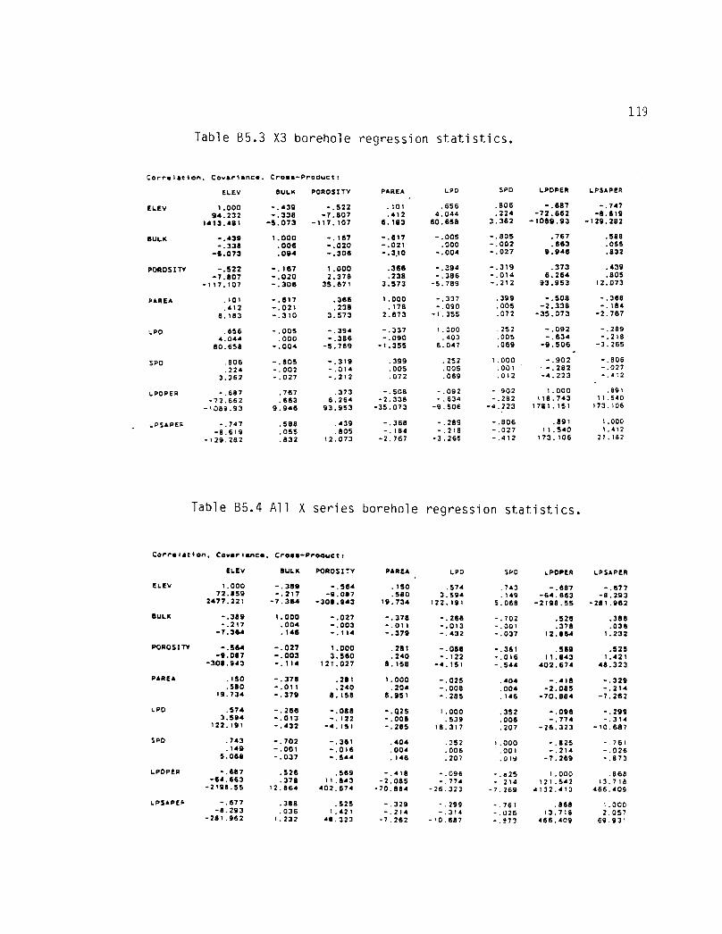
Table B5.3 X3 borehole regression statistics.

Corrolation. Covarianc4i. 0rosa-ProBuct:

ELEY BULK POROSITY PAREA LPG,

ELEV 1.000 -.439 -.522 .101 .656 .806 - .687 -.747

94.232 -.338 -7.807 .412 4.044 .224 -72.662 -8.619

1413.481 -5.073 -117.107 6.183 60.658 3.362 -1089.93 -129.282

BULK - .439 1.000 - .167 - .617 - .005 - .805 .767 .588

-.338 .006 -.020 -.021 .000 -.002 .663 .055

-6.073 .094 -.306 -.310 -.004 -.027 9.946 .832

POROSITY -.522 -.167 1.000 .366 -.394 -.319 .373 .439

-7.807 -.020 2.378 .238 - .386 - .014 6.264 .805

-117.107 -.306 35.671 3.573 -5.789 -.212 93.953 12.073

PAREA .101 - .617 .366 1.000 -.337 .399 -.508 -.368

.412 -.021 .238 .178 -.090 .005 -2.338 - .184

8.183 -.310 3.573 2.673 -1.355 .072 -35.073 -2.767

656 -.005 -.394 -.337 1.000 .252 -.092 -.289

4 .044 .000 -.386 -.090 .403 .005 -.634 -.218

60.658 - .004 -5.789 -1.355 6.047 .069 -9.506 -3.265

806 -.805 -.319 .399 .252 1.000 -.902 - .806

.224 -.002 -.014 .005 .005 .001 - .282 -.027

3.362 -.027 -.212 .072 .069 .012 -4.223 -.412-

-.687 .767 .373 -.508 -.092 -.902 1.000 .891

-72.662 .663 6.264 -2.338 -.634 -.282 118.743 11.540

- 1089.93 9.946 93.953 - 35.073 - 9.506 - 4.223 1781.151 173.106

119

SPD LPOPER LPSAPER

LPO

SPO

LPDPER

LPSAPER- .747 .588 .439-8.619 .055 .805

-129.282 .832 12.073

-.368-.184

-2.767

-.289-.218

-3.265

- .806-.027-.412

.891 1.000

11.540 1.412

173.106 21.182

Table B5.4 All X series borehole regression statistics.

Corrolacion. Coveriance. Cross-Product:

[LEY SULK POROSITY PAREA LPO SPO LPOPER LPSAPER

ELEV 1.000 -.389 -.564 .150 .674 .743 -.687 -.677

72.859 -.217 -9.067 .580 3.594 .149 - 64.863 -8.293

2477.221 -7.364 -308.943 19.734 122.191 5.068 -2198.55 -281.962

SULK -.389 1.000 -.027 -.378 -.266 -.702 .526 .386

- .217 .004 -.003 -.011 -.013 - .001 .378 .036

-7.364 .146 -.114 -.379 - .432 - .037 12.864 1,232

POROSITY -.564 -.027 1.000 .281 -.088 - .361 .569 .525

-9.087 -.003 3.560 .240 -.122 -.016 11.843 1.421

-308.943 -.114 121.027 8.158 -4.151 -.544 402.674 48.323

PAREA .150 -.378 .281 1.000 -.025 .404 - .416 -.329

.580 -.011 .240 .204 -.008 .004 -2.085 -.214

19.734 -.379 8.158 6.951 -.285 .146 -70.884 -7.262

LPO .574 -.266 -.088 -.Q25 1.000 .352 -.096 -.299

3.594 -.013 -.122 -.008 .539 .006 -.774 -.314

122.191 -.432 -4.151 -.285 18.317 .207 -26.123 - 10.687

SPD .743 - .702 - .361 .404 .352 1.000 -.825 - 761

.149 -.001 -.016 .004 .006 .001 -.214 -.0265.066 - .037 - .544 .146 .207 .01Y -7.269 -.873

LPOPER -.687 .526 .569 -.416 -.096 -.625 1.000 .868

-64.663 .378 11.943 - 2.085 -.774 -.214 121.542 13.716

-2198.55 12.864 402.674 -70.884 -26.323 -7.269 4132.413 466.409

LPSAPEA -.677 .388 .525

-8.293 .036 1.421-281.962 1.232 48.323

-.329-.214

- 7 .262

-.299-.31A

- , 0.687

-.761-.026-.973

.86813.716

466.409

1.0002.057

69.931

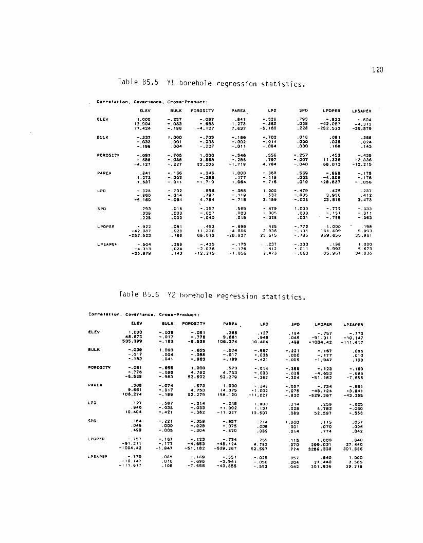
120

Table B5.5 Y1 borehole regression statistics.

Correlation. Covariance. Cross-Product:

ELEV

BULK POROSITY PAREA, LPD

SPD LPDPER LPSAPER

ELEV

1.000 -.337 -.097 .841 -.328 .793 -.922 -.504

12.904 -.033 -.688 1.273

-.860 .038 -42.087 -4.313

77.424 -.198 -4.127 7.637

-5.160 .228 -252.523 -25.879

BULK -.337 1.000 -.705 -.166 -.702 .018 .081 .368

-.033 .001 -.038 -.002 -.014 .000 .028 .024

-.198 .004 -.227 -.011 -.084 .000 .168 .143

POROSITY -.097 -.705 1.000 -.346 .556 -.257 .453 -,435

-.688 -.038 3.868 -.286 .797 -.007 11.336 -2.036

-4.127 -.227 23.205 -1.719 4.784 -.040 68.013 -12.215

PAREA .841 -.166 -.346 1.000 -.388 .569 -.898 -.175

1.273 -.002 -.286 .177 -.119 .003 -4.806 -.176

7.637 -.011 -1.719 1.084 -.716 .019 -28.837 -1.056

LPO -.328 -.702 .558 -.388 1.000 -.479 .425 .237

-.860 -.014 .797 -.119 .532 -.005 3.938 .412

-5.160 -.084 4.784 -.716 3.189 -.028 23.615 2.473

SPD .793 .018 -.257 .569 -.479 1.000 -.772 -.333

.038 .000 -.007 .003 -.005 .000. -.131 -.011

.228 .000 -.040 .019 -.028 .001 -.785 -.063

LPOPER -.922 .081 .463 -.898 .425 -.772 1.000 ' .198

-42.087 .028 11.336 -4.806 3.936 -.131 161.609 5.993

-252.523 .168 68.013 -28.837 23.615 -.785 969.656 35.961

LPSAPEt -.504 .368 -.435 -.175 .237 -.333 .198 1.000

-4.313 .024 -2.036 -.176 .412 -.011 5.993 5.673

-25.879 .143 -12.215 -1.056 2.473 -.063 35.961 34.036

Table 13 5.6 Y2 borehole regression statistics.

Correlation. Covariance. Cross-Product:

ELEV BULK POROSITY PAREA • LPO SPO LPOPER LPSAPER

ELEV 1.000 -.039 -.051 .385 .127 .184 -.757 -.770

48.673 - .017 - .776 9.661 .948 .045 -91.311 - 10.147

535.399 - .183 -8.538 108-274 10.404 .499 -1004.42 -111.817

SULK -.039 1.000 - .655 - .074 - .587 - .221 - .167 .085- .017 .004 - .088 -.017 -.038 .000 -.177 .010

-.183 .041 - .963 - .189 - .421 -.005 -1.947 .108

POROSITY -.051 -.855 1.000 .573 -.014 -.358 -.123 -.169

-.778 -. 088 4.782 4.753 -.033 - .028 -4.653 -.698

-8.538 -.963 52.602 52.279 -.362 -.304 -51.182 -7.656

PAREA .365 -.074 .573 1.000 -.248 -.557 -.734 -.551

9.661 -.017 4.753 14.375 -1.002 -.075 -48.124 -3.941

106.274 -.189 52.279 158.120 -11.027 -.820 -529.367 -43.355

LPD .127 -.587 -.014 -.248 1.000 .214 .259 -.025

.946 -.038 -.033 -1.002 1.137 .008 4.782 -.050

10.404 - .421 -.362 -11.027 12.507 .089 52.597 -.553

.184 -.221 -.358 -.557 .214 1.000 .115 .057SPO

.045 .000 -.028 -.075 .008 001 .070 .004

.499 -.005 -.304 -.820 .089 .014 .774 .042

LPDPER -.757 -.167 -.123 -.734 .259 .115 1.000 .840

-91.311 -.177 -4.653 -48.124 4.782 .070 299.031 27.440

-1004.42 -1.947 -51.182 -529.367 52.597 .774 3289.338 301.836

LPSAPER -.770 .085

-10.147 .010

-111.617 .108

-.169 -.551 -.025 057 .840 1.000

-.696 -3.941 -.050 .004

27.440 3.565

-7.656 -43.355 -.553 .042

301.836 39.219

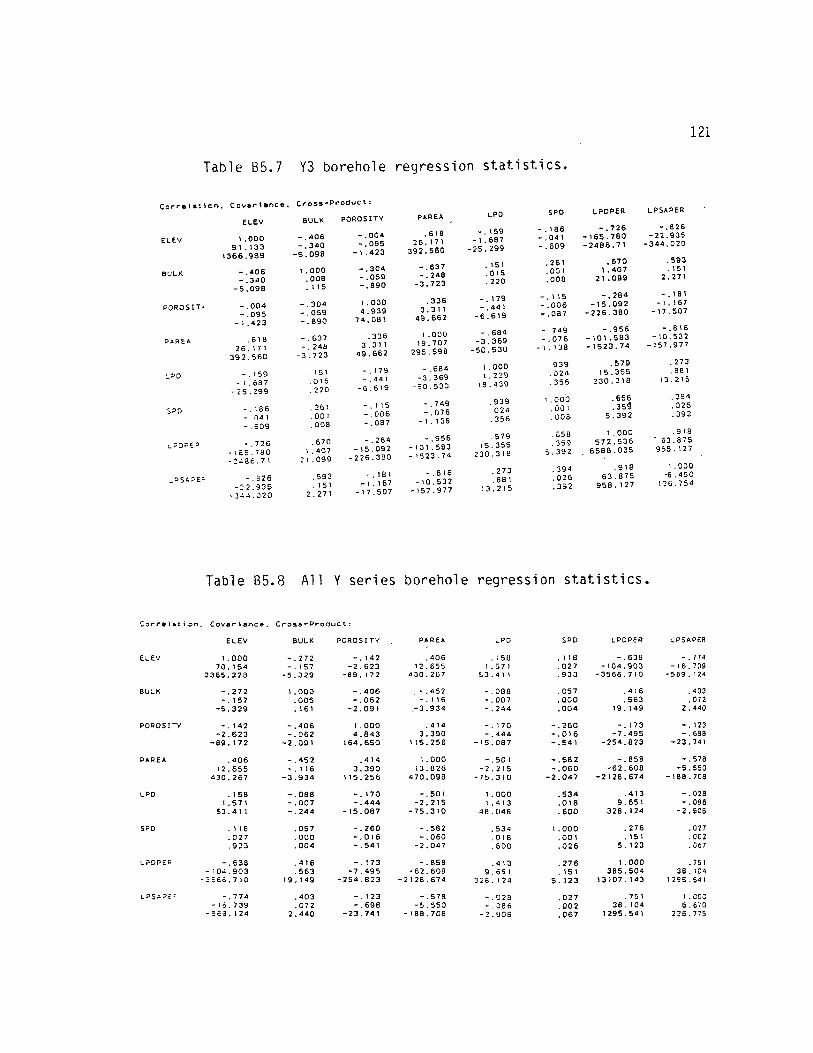
-.159 .151

-1.687 .015

-25.299 .220

-.186 .261

- 041 .001

-.609 .008

-.726 .670

-1E5.780

1.407

-2486.71

21.099

.593

.151

2.271

LPO

SPO

LPOPEP

_PSAPEP -.326

-:2.935-844.020

LPD

SPO LPDPER LPSAPER

-.159-1.687-25.299

.151

.015

.220

-.179-.441

-6.619

-.68 4

-3.369-50.530

1.0001.229

18.439

.261

.001

.008

-.115

-.006-.087

-,749-.076-1.138

.939

.024

.356

.6701.407

21.099

-.28 4

-15.092-226.380

-.956-101.583

-1523. 74

.579

f5.355

230.318

-.826-22.935-344,020

.593

.1512.27t

-.181-1.167

-17.507

-.816-10.532-157.977

.273

.88113.215

- .1a6 -.726

-.041 -165.780

-.609 -2486.71

-.115 -.749 .939 1.000 .658 .394

-.006 -.076 .024 .001 .354 .026

-.087 - 1 .138 .356 .006 5.392 .392

- .284

-15.092

-226.380

-.956-101.583-1523.7 4

.579

15.355230.318

.658

.3595.392

1.000

572.5368588.035

.018

- 63.875959.127

-.181 -.816

-1.167 -10.532

-17.507 -157.977

.273

.88113.215

.39 4

.026

.392

.918

63.875956.127

1.000

126.754

Table 85.7 Y3 borehole regression statistics.

Correlaticn. Covariance. Cross-Producf:

ELEV BULK POROSITY PAREA

ELEV 1.000 -,406 -.004 ,6 1 8

91.133 -.340 -.095 26.171

1366.989 -5.098 -1.423 392.560

BULK -.406 1.000 -.304 -,637

-.340 .008 -.059 -.248

-5.098 .115 -.890 -3.723

POR0S1T , -.004 -.304 1.000 .336

-.095 -.059 4.939 3.311

-1.423 -.890 74.081 49.662

PAREA .618 -.637 .336 1.000

26.171 -.248 3.311 19.707

392.560 -3.723 49.662 295.598

-.684

-.441

-3.369

-6.619

-50.530

121

Table 85.8 All Y series borehole regression statistics.

Correlltion. Covariance.

ELEV

Cross-Product:

BULK POROSITY PARES LPD SPD LPDPER LPSAPER

ELEV 1.000 -.272 -.142 ,406 ..58 .118 -.638 -.774

70.154 -.157 -2.623 12.655 1.571 .027 -104.903 -16.739

23135.228 -5.329 -89.172 430.267 53.411 .933 -3566.710 -569.124

BULK -.272 1.000 -.406 -.452 -.088 .057 .416 .403

-.157 .005 -.062 -.116 -.007 .000 .563 .072

-5.329 .161 -2.091 -3.934 -.244 .004 19.149 2.440

POROSITY -.142 -.406 1.000 .414 -.170 -.260 -.173 -.123

-2.623 -.062 4.843 3.390 -.444 -.016 -7.495 -.698

-89.172 -2.091 164,650 115.256 -15.087 -.541 -254.823 -23.741

PARES .406 -.452 .414 1.000 -.501 -.582 -.858 -.578

12.655 -.116 3.390 13.826 -2.215 -.060 -62.608 -5.550

430.267 -3.934 115.256 470.098 -75.310 -2.047 -2128.674 -188.708

LPO .158 -.088 -.170 -.501 1.000 .534 .413 -.028

1.571 -.007 - .444 -2.215 1.413 .018 9.651 -.086

53.411 -.244 -15.087 -75.310 48,048 .600 328.124 -2.908

590 .11 8 .057 -.260 .582 .534 1.000 .276 .027

.027 .000 -.016 .060 .018 .001 .151 .002

.933 .004 -.541 -2.047 .600 .026 5.123 .067

LPDPEP -.638 .416 -.173 -.858 ,413 .276 1.000 .751

- 1 04.903 .563 -7.495 -62.608 9.651 .151 385.504 38.104- 3565.710 19.149 -254.823 -2128.674 328.124 5.123 13107.143 1295.541

LPSAPE: -.774 .403 -.123 .578 -.028 ,027 .751 1.000-16.739 .072 -.698 -5.550 -.086 .002 38.104 6.670

-568.124 2.440 -23.741 -188.708 -2.908 .067 1295.541 226.775

Table B5.9 71 borehole regression statistics.

Correlation. Covariance. Cross-Product:

ELEV BULK POROSITY

PAREA • LPD SPO LPDPER LPS4PER

122

ELEV 1.000 -.338 .059 n .802

12.795 -.058 .347 1.949

76.768 -.350 2.084 11.695

BULK -.338 1.000 -.591 -.549- .058 .002 -.047 -.018

-.350 .014 -.283 -.108

-.257 .906 -.954 -.810

-.350 .059 -43.181 -4.904

-2.098 .357 -259.084 -29.424

-.796 -.128 .425 .588

-.015 .000 .261 .048

-.088 -.001 1.563 .289

POROSITY .059 -.591 1.000 .583 .371

-.035

-.063 -.028

.347 -.047 2.732 .655 .234

-.001

-1.309 -.079

2.084 -.203 16.390 3.932

1.402

-.006

-7.857 -.473

PARES .802 -.549 .583 1.000

1.949 -.018 .655 .462

11.695 -.108 3.932 2.773

LPD -.257 -.796 .371 -.033

-.350 -.015 .234 -.009- 2.098 -.088 1.402 -.051

-.033 715 -.809 -.671

-.009 .009 -6.963 -.772

- .051 .053 -41.778 -4.632

1.000 -.409 .120 -.179

.145 -.003 .577 -.115

.869 -.017 3.462 -.691

SPD .906 -.128 -.035 .715

-.409

1.000

-.842 -.650

.059 .000 -.001 .009

-.003

.000

-.196- -.020

.357 -.001 -.006 .053

- .017 .002

-1.174 -.121

LPOPER -.954 .425 -.063 -.809 .120

-.842

1.000 .933-43.181 .261 -1.309 -6.963 .577

-.196

160.248 20.002

-259.084 1.563 -7.857 -41.778

3.462

-1.174

961.487 120.012

LPSAPE,, -.910 .588 -.028 -.671

-.179 -.650 .933 1.000-4.904 .048 -.079 -.772

-.115 -.020

20.002 2.865

- 29.424 .289 -.473 -4.632

-.691 -.121

120.012 T7.193

Table B5.10 72 borehole regression statistics.

Correlation, Covariance, Cross-Product.

ELEV

BULK POROSITY PAREA

LPD

SPD LPDPER LPSAPER

ELEV 1.00049.184

541.019

.072

.036

.399

-.469-32.381

-356.188

.7362.591

28.497

.5523.290

36.186

.728 -.779 -.813

.088 -82.495 -11.733

.973 -907.440 -129.059

BULK .072 1.000 .208 -.236 -.069 -.260 .243 .135

.036 .005 .148 -.009 -.004 .000 .265 .020

.399 .057 1.623 -.094 -.047 -.004 2.913 .221

POROSITY -.469 .208 1.000 -.284 -.372 -.329 .691 .298

-32.381 .148 96.731 -1.300 -3.111 -.056 102.582 6.032

-356.188 1.623 1064.041 -14.301 -34.221 -.616 1128.401 66.355

PAREA .736 -.236 -.264 1.000 .424 779 -.865 -.946

2.591 -.009 -1.300 .252 .181 .007 -6.552 -.977

28.497 -.094 -14.301 2.768 1.992 .074 -72.077 -10.749

LPD .552 -.069 -.372 .424 1.000 .285 -.446 -.530

3.290 -.004 -3.111 .181 .723 .004 -5.731 -.927

36.186 -.047 -34.221 1.992 7.955 .046 -63.046 -10.199

SPO .728 -.260 -.329 .779 .285 1.000 -.765 -.759

.088 .000 -.056 .007 .004 000 -.200 -.027

.973 -.004 -.616 .074 .046 .003 -2.200 -.298

LPOPER -.779 .243 .691 -.865 -.446 -.765 1.000 .847- 52.495 .265 102.582 -6.552 -5.731 -.200 227.964 26.333

-937.440 2.913 1128.401 -72.077 -63.046 -2.200 2507.603 289.665

LPSAPE:. -.513 .135 .298 -.946 -.530 -.759 .847 1.000- 11.733 .020 6.032 -.977 -.927 -.027 26.333 4.237

-129.059 .221 66.355 -10.749 -10.199 -.298 289.665 46.605

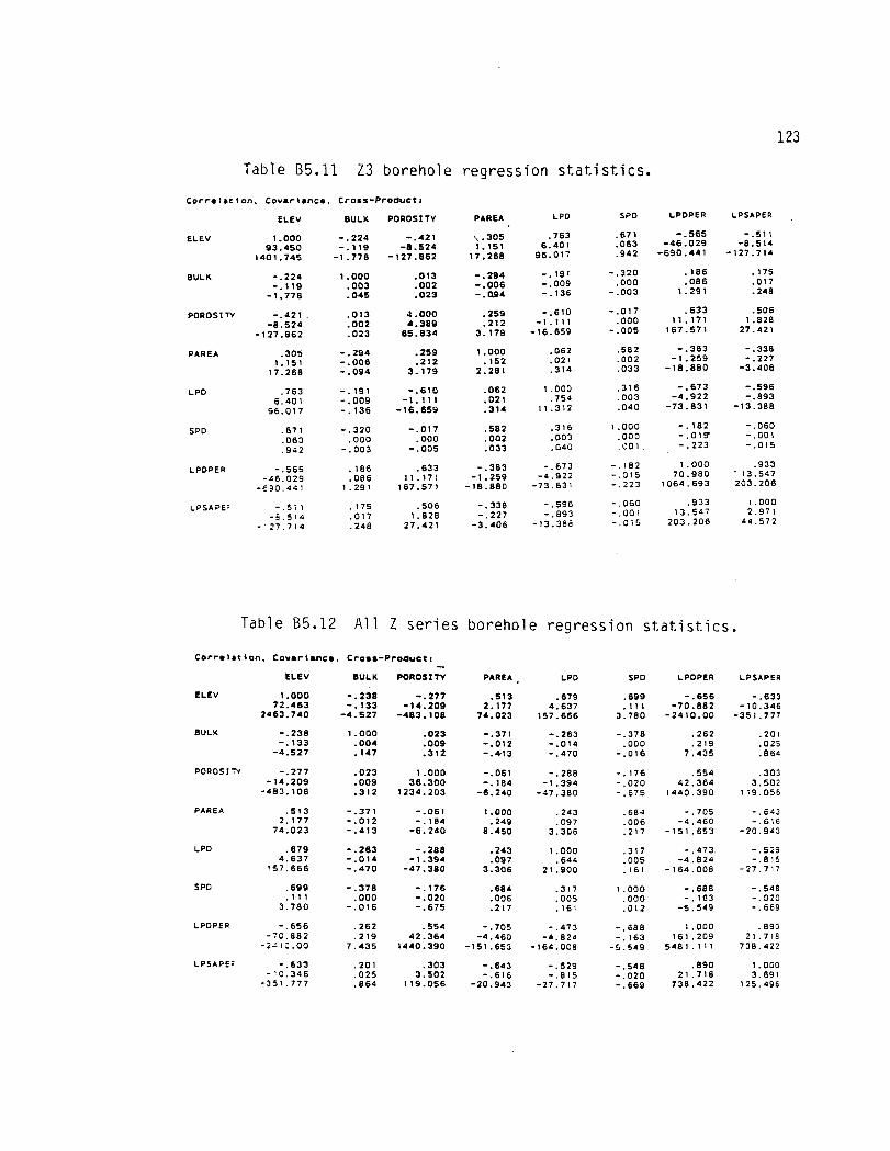
Et. EV BULK POROSITY PAREA LPO 5P0 LPDPER LPSAPER

.582

.002

.033

.062

.021

.31 4

-.383 -.338

-1.259 -.227

-18.880 -3.406

Table B5.12 All Z series borehole regression statistics.

Correlation. Covariance. Cross-Product:

BULK POROSITY PAREA • LIDD SPD LPDPER LPSAPERELE V

-,643-.616

-20.943

.513 -.371 -.061 1.000 .243 .684 -.705

2.177 -.012 -.184 .249 .097 .006 -4.460

74.023 -.413 -6.240 8.450 3.306 .217 -151.653

.89021. 718

738.422

- .656 .262 .554 -.705 -.473 -.688 1.000

- 7 0.882 .219 42.364 -4.460 -4.824 -.163 161.209

-2 4 10.00 7.435 1440.390 -151.653 -164.008 -5.549 5481.111

Table B5.11 Z3 borehole regression statistics.

Correlation, Covariance, Cross-Product:

1.000 -.224 -.421

93.450 -.119 -8.524

1401.745 -1.778 -127.862

.763 .671 -.565 -.511

1.151 6.401 .063 -46.029 -8.514

17.268 96.017 .942 -690.441 -127.714

ELEV

-.224 1.000 .013 -.294

-.119 .003 .002 -.006

-1.778 .045 .023 -.494

-.421 .013 4.000 .259

-8.524 .002 4.389 .212

-127.862 .023 65.834 3.179

.305 -.294 .259 1.000

1.151 -.006 .212 .152

17.268 -.094 3.179 2.281

-.191 -.320 .186 .175

-.009 .000 .086 .017

-.136 -.003 1.291 .248

-.610 -.017 .633 .506

-1.111 .000 11.171 1.828

-16.659 -.005 167.571 27.421

1.000 -.238 -.277 .513 .679 .699 -.656 -.633

72.463 -.133 -14.209 2.177 4.637 .111 -70.882 -10.346

2463.740 -4.527 -483.108 74.023 157.666 3.780 -2410.00 -351.777

-.238 1.000 .023 -.371 -.263 -.378 .262 .201-.133 .004 .009 -.012 -.014 .000 .219 .025-4.527 .147 .312 -.413 -.470 -.016 7.435 .864

-.277 .023 1.000 -.061 -.288 -,176 .554 .303

-14.209 .009 36.300 -.184 -1.394 -.020 42.364 3.502

-483.108 .312 1234.203 -6.240 -47.380 -.675 1440.390 119.056

.879 -.263 -.288 .243 1.000 .317 -.473 -.529

4.637 -.014 -1.394 .097 .644 .005 -4.824 -.815157.666 -.470 -47.380 3.306 21.900 .161 -164.008 -27.717

.699 -.378 -.176 .884 .317 1.000 -.688 -.548

.111 .000 -.020 .006 .005 .000 -.163 -.020

3.760 -.016 -.675 .217 .161 .012 -5.549 -.669

-.633 .201 .303 -.643 -.529 -.548 .890 1.000

-'0.346 .025 3.502 -.616 -.815 -.020 21.718 3.691

-351.777 .864 119.056 -20.943 -27.717 -.669 738.422 125.496

123

-.182-.015-.223

-.673-4.922-73.83 1

.933- 13.547203.206

-.565-46.029

-690.441

1.00070.980

1064.693

.186 .633 -.383

.086 11.171 -1.259

1.291 167.571 -18.880

1.0002.971

44.572

-.060-.00 1

-.015

.93313.647

203.206

-.511-8.514

-127.714

.175 .506 -.338 -.596

.017 1.828 -.227 -.893

.248 27.421 -3.406 -13.388

.763 -.191 -.610 .062 1.000 .316 -.673 -.596

6.401 -.009 -1.111 .021 .754 .003 -4.922 -.893

96.017 -.136 -16.659 .314 11.312 .040 -73.831 -13.388

.671 -.320 -.017 .582

.063 .000 .000 .002

.942 -.003 -.005 .033

.316

.003

.040

-.060- .001-.015

-.182-.016-.223

1.000.000.001.

BULK

POROSITY

PAREA

LPD

SPD

LPDPER

LPSAPE;

ELEV

BULK

POROSI7v

PAR 64

LPD

SPD

LPDPER

LPSAPE;

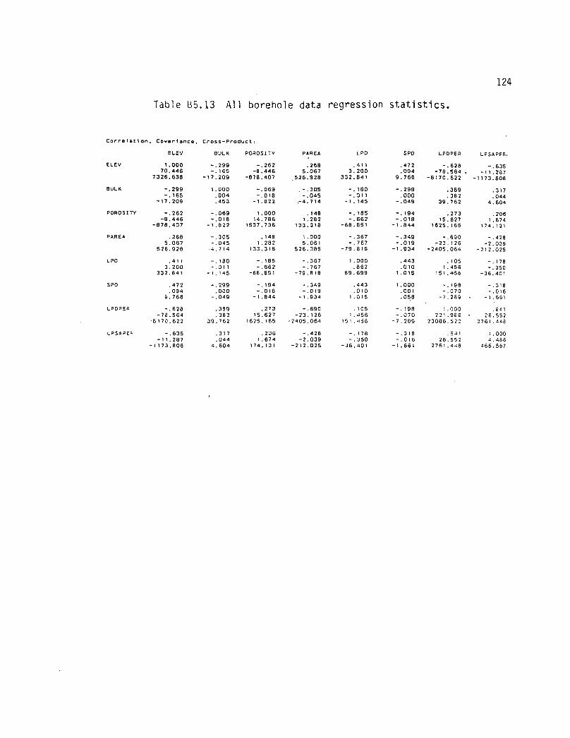
124

Table B5.13 All borehole data regression statistics.

Correlation, Covariance. Cross-Product;

ELEV BULK POROSITY PAREA LPD SPD LPDPER LOSAPER.

ELEV 1.000 -.299 -.262 .268 .411 .472 -.628 -.635

70.448 -.165 -8.446 5.067 3.200 .094 -78.564 -11.287

7326.638 -17.209 -878.407 526.928 332.841 9.766 -8170.622 -1173.808

BULK -.299 1.000 -.069 -.305 -.180 -.299 .389 .317

-.165 .004 -.018 -.045 -.011 .000 .382 .044

-17.209 .453 -1.822 ,4.7141 -1.145 -.049 39.762 4.604

POROSITY -.262 -.069 1.000 .148 -.185 -.194 .273 .208

-8.446 -.018 14.786 1.282 -.662 -.018 15.627 1.674

-878.407 -1.822 1537.736 133.318 -68.851 -1.844 1625.165 174.131

PAREA .268 -.305 .148 1.000 -.367 -.349 -,690 -.428

5.067 -.045 1.282 5.061 -.767 -.019 -23.126 -2.039

526.928 -4.714 133.318 526.385 -79.81E1 -1.934 -2405.064 -212.025

LPO .411 -.180 -.185 -.367 1.000 .443 .105 -.178

3.200 -011 -.662 -.767 .862 .010 1.456 -.350

332.841 -1.145 -68.851 -79.818 89.699 1.015 151.456 -36.401

SPD .472 -.299 -.194 -.349 .443 1.000 -.198 -.318

.094 .000 -.018 -.019 .010 .001 -.070 -.016

9.766 -.049 -1.844 -1.934 1.015 .058 -7.269 -1.661

LPDPER -.628 .389 .273 -.690 .105 -.198 1.000 .641

-70.564 .382 15.627 -23.126 1.456 -.070 221.966 26.552

-6170.622 39.762 1625.165 -2405.064 ISi.459 -7.289 23086.522 2761.448

LPSAPE: -.635 .317 .206 -.428 -.178 -.318 .841 1.000

-1 1 .287 .044 1.674 -2.039 -.350 -.016 26.552 4.486

-1173.808 4.604 174.131 -212.025 -36.401 -1.661 2761.448 466.567

APPENDIX C

CALIBRATION RESULTS FROM PORESIZER

An explanation of calibration techniques and instrumentperformance is included in this appendix.

125

126

C.1 Poresizer Calibration

Over the course of this study, several penetrometers were used in

the testing procedure. Each new penetrometer was inspected visually and

by the poresizer before it was used for intrusion testing. Blank

penetrometers were sealed, evacuated and filled with mercury to check

manufacturer supplied penetrometer volumes.

Silica-alumina pellets were obtained from the manufacturer for

instrument calibration purposes. The poresizer is checked after every 50

intrusion tests to ensure proper performance. Table C.1 shows the

results of the latest test with those from the manufacturer. All

parameters are within acceptable limits. The underestimation of pore

area and over estimation of median pore diameter probably stems from the

fact that intrusion pressures only reached 187 MPa instead of the listed

207 MPa.

TABLE C.1 Calibration results of Poresizer 9310 using silica-aluminapellets.

MANUFACTURER STUDYTOTAL INTRUSION VOLUME (cm 3/gm) 0.33 + .05 0.353TOTAL PORE AREA ( m2/ gm ) 75 -47- 10 61.2MEDIAN PORE DIAMETER (VOLUME) (um) 0.03 17 .005 0.112MEDIAN PORE DIAMETER (AREA) (um) 0.01 .002 0.009

C.2 Sample Variability

Because of the destructive nature of intrusion testing it is near

impossible to retest the same sample. Samples from the same core

location, only adjacent to each other, were tested for comparison and as

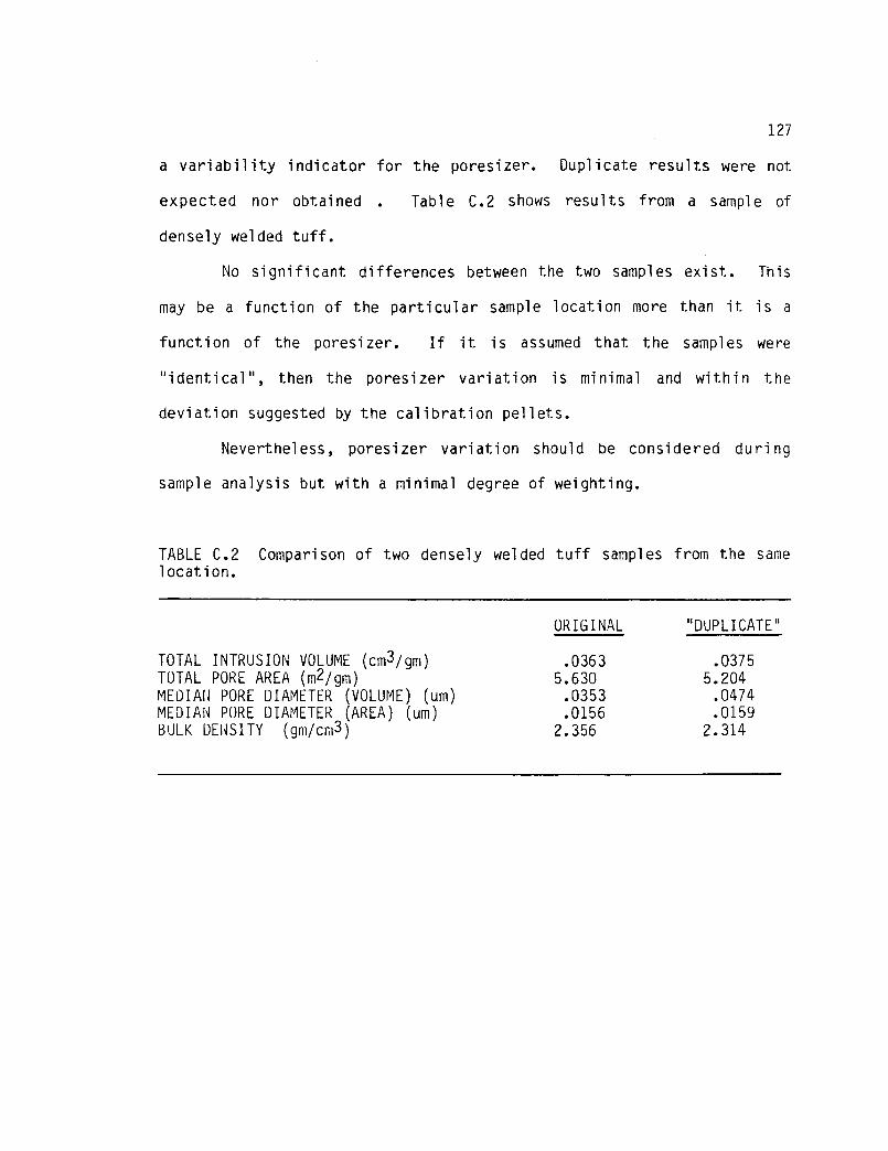
127

a variability indicator for the poresizer. Duplicate results were not

expected nor obtained . Table C.2 shows results from a sample of

densely welded tuff.

No significant differences between the two samples exist. This

may be a function of the particular sample location more than it is a

function of the poresizer. If it is assumed that the samples were

"identical", then the poresizer variation is minimal and within the

deviation suggested by the calibration pellets.

Nevertheless, poresizer variation should be considered during

sample analysis but with a minimal degree of weighting.

TABLE C.2 Comparison of two densely welded tuff samples from the samelocation.

ORIGINAL "DUPLICATE"

TOTAL INTRUSION VOLUME (cm 3/gm) .0363 .0375TOTAL PORE AREA ( m2/ gm ) 5.630 5.204MEDIAN PORE DIAMETER (VOLUME) (um) .0353 .0474MEDIAN PORE DIAMETER (AREA) (um) .0156 .0159BULK DENSITY (gm/cm 3 ) 2.356 2.314

REFERENCES

De Boer, J.H., The Shapes of Capillaries, in The Structure andproperties of Porous Materials, ed., Everett, D.H., and F.S. Stone, Colston Research Society, Butterworths ScientificPublications, London, pp. 68 - 94, 1958.

Evans, D.D., Unsaturated Flow and Transport Through Fractured RockRelated to High-Level Waste Repositories, Progress Report toU.S. Nuclear Regulatory Commission, 1988.

Geomath, Variogram Computation Program, GAM3D and variogram plottingprogram, VPLOT2, Lakewood, Colorado, 1987.

Good, R.J., and R.Sh. Mikhail, The Contact Angle in Mercury IntrusionPorosimetry, Powder Technology, pp. 53 - 62, Vol. 29, 1981.

Hillel, D., Fundamentals of Soil Physics, Academic Press, NewYork, 1980.

Journel, A.G., and CH. J. Huijbregts, Mining Geostatistics, AcademicPress, New York, 1978.

Joyner, L.G., Barrett, E.P. and R.J. Skold, The Determination of PoreVolume and Area Distributions in Porous Substances.Comparison between Nitrogen Isotherm and Mercury PorosimeterMethods, J.Am. Chem. Soc. 73., 3155-58 July (1951).

Kim, Y.C., Geostatistics in Ore Reserve Estimation and Mine Planning,Course Notes, Department of Mining and Geological Engineering,University of Arizona, Tucson, Arizona, December 1982.

Kim, Y.C., Department of Mining and Geological Engineering, Universityof Arizona, Tucson, Arizona, personal communication, 1988.

Klar, E., Relations between Pore Characteristics and CompactingProperties of Copper Powders, in H.H. Hausner, ed., Perspectivesin Powder Metallurgy, Vol. 6, 1971.

Klavetter, E.A., and R.R. Peters, An Evaluation of the Use of MercuryPorosimetry in Calculating Hydrologic Properties of Tuffs FromYucca Mountain, Nevada, SAND86-0286, Sandia NationalLaboratories, Albuquerque, NM, 1987.

Kloubek, J., Hysteresis in Porosimetry, Powder Technology, pp. 63 - 73,Vol. 29, 1981.

128

129

Kloubek, J., A New Method for the Investigation of Porous Structuresusing Mercury Porosimetry, Powder Technology, pp. 89 - 97, Vol.29, 1981.

Matheron, G., The Intrinsic Random Functions and Their Applications,Adv. App. Prob., pp. 239-465, Vol. 5, 1973.

Micromeritics Instruction Manual for Poresizer 9310, June 1986.

Miller, I., and J.E. Freund, Probability and Statistics for Engineers,Prentice-Hall, Inc., Englewood Cliffs, New Jersey, 1977.

Modry, S., Svata M. and J. Van Brakel, Thematic Bibliography ofMercury Porosimetry, Powder Technology, pp. 13 - 43, Vol 29,1981.

Moscou, L., and S. Lub, Practical Use of Mercury Porosimetry in theStudy of Porous Solids, Powder Technology, pp. 45 - 52, Vol. 29,1981.

Peterson, D.W., Dacitic Ash-Flow Sheet near Superior and Globe,Arizona, Stanford Univ., Stanford, California, Ph. D. thesis,130 p.; U.S. Geological Survey open-file report, 130 p., April3, 1961.

Peterson, D.W., Zoned Ash-Flow Sheet in the Region Around Superior,Arizona, in S. Titley, ed., Arizona Geological Society, SouthernArizona Guidebook, III, Tucson, Arizona, April 11-13, 1968.

Pickell, J.J., Swanson, B.F., and W.B. Hickman, Application of Air-Mercury and Oil-Air Capillary Pressure Data In the Study of PoreStructure and Fluid Distribution, Society of Petroleum EngineersJournal, pp. 55 - 61, Vol. 237, 1966.

Rahi, K. A., Hydraulic Conductivity Assessment for a Variably- SaturatedRock Matrix, University of Arizona, Tucson Arizona, MastersThesis, Department of Hydrology and Water Resources, 1986.

Rasmussen, T. C. and D. D. Evans, Unsaturated Flow and Transport ThroughFractured Rock - Related to High-Level Waste Repositories -Phase II, NUREG/CR-4655, U. S. Nuclear Regulatory Commission,pp. 475, 1986.

Ritter, H.L., and L.C. Drake, Pore-Size Distribution in PorousMaterials: Pressure Porosimeter and Determinations of CompleteMacropore-Size Distribution, Ind. Eng. Chem. Anal. Ed., 17, 782(1945).

Rootare, H.M., and C.F. Prenzlow, Surface Areas from Mercury PorosimeterMeasurements, The Journel of Physical Chemistry, Vol. 71, No. 8,July 1967.

130

Ternan, M., and 0.M. Fuller, A Comparison of Methods Used to MeasurePore Size in Solids, The Canadian Journel of ChemicalEngineering, Vol. 57, pp. 750 - 757, December, 1979.

Van Brakel, J., Modry, S., and M. Svata, Mercury Porosimetry:State of the Art, Powder Technology, pp. 1 - 12, Vol. 29, 1981.

Wardlaw, N.C., and R.P. Taylor, Mercury Capillary Pressure Curves andthe Interpretation of Pore Structure and Capillary Behavior inReservoir Rocks, Bulletin of Canadian Petroleum Geology, Vol.24, No. 2, pp. 225 - 262, 1976.

Warrick, A.W., Myers, D.E., and D.R. Nielsen, Geostatistical MethodsApplied to Soil Science, pp. 53 - 81, in Methods of SoilAnalysis, Part I. Physical and Mineralogical Methods, Am. Soc.of Agronomy, Inc., Soil Science Society of America, Inc.,Madison, WI., 1986.

Washburn, E.W., Note on a Method of Determining the Distribution of PoreSizes in a Porous Material, National Academy of ScienceProceedings, Vol. 7, p. 115, 1921.

Weber, D.S., Stable Isotopes of Authigenic Minerals in VariablySaturated Fracturated Tuff, University of Arizona, TucsonArizona, Masters Thesis, Department of Hydrology and WaterResources, 1986.

Whittemore, 0. 3 ., Mercury Porosimetry of Ceramics, Powder Technology,pp. 167 - 175, Vol. 29, 1981.

Winslow, D.N., and C.W. Lovell, Measurements of Pore Size Distributionsin Cements, Aggregates and Soils, Powder Technology, pp. 151 -165, Vol. 29, 1981.

Yeh, T. C., Rasmussen, T. C. and D. D. Evans, Simulation of Liquid andVapor Movement in Unsaturated Fractured Rock at the Apache LeapTuff Site - Models and Strategies, NUREG/CR-5097, U. S. NuclearRegulatory Commission, pp. 73, 1988.