
Provided for non-commercial research and educational...
18
Provided for non-commercial research and educational use only. Not for reproduction, distribution or commercial use. This article was originally published in the Encyclopedia of Biodiversity, second edition, the copy attached is provided by Elsevier for the author’s benefit and for the benefit of the author’s institution, for non-commercial research and educational use. This includes without limitation use in instruction at your institution, distribution to specific colleagues, and providing a copy to your institution’s administrator. All other uses, reproduction and distribution, including without limitation commercial reprints, selling or licensing copies or access, or posting on open internet sites, your personal or institution’s website or repository, are prohibited. For exceptions, permission may be sought for such use through Elsevier’s permissions site at: http://www.elsevier.com/locate/permissionusematerial Gotelli Nicholas J., and Chao Anne (2013) Measuring and Estimating Species Richness, Species Diversity, and Biotic Similarity from Sampling Data. In: Levin S.A. (ed.) Encyclopedia of Biodiversity, second edition, Volume 5, pp. 195- 211. Waltham, MA: Academic Press. © 2013 Elsevier Inc. All rights reserved.
-
Upload
truonglien -
Category
Documents
-
view
218 -
download
1
Transcript of Provided for non-commercial research and educational...

Provided for non-commercial research and educational use only. Not for reproduction, distribution or commercial use.
This article was originally published in the Encyclopedia of Biodiversity, second edition, the copy attached is provided by Elsevier for the author’s benefit and for the benefit of the author’s institution, for non-commercial research
and educational use. This includes without limitation use in instruction at your institution, distribution to specific colleagues, and providing a copy to your institution’s administrator.
All other uses, reproduction and distribution, including without limitation commercial reprints, selling or licensing copies or access, or posting on open internet sites, your personal or institution’s website or repository, are prohibited.
For exceptions, permission may be sought for such use through Elsevier’s permissions site at:
http://www.elsevier.com/locate/permissionusematerial
Gotelli Nicholas J., and Chao Anne (2013) Measuring and Estimating Species Richness, Species Diversity, and Biotic Similarity from Sampling Data. In: Levin S.A. (ed.) Encyclopedia of Biodiversity, second edition, Volume 5, pp. 195-
211. Waltham, MA: Academic Press.
© 2013 Elsevier Inc. All rights reserved.
Author's personal copy
En
Measuring and Estimating Species Richness, Species Diversity, and BioticSimilarity from Sampling DataNicholas J Gotelli, University of Vermont, Burlington, VT, USAAnne Chao, National Tsing Hua University, Hsin-Chu, Taiwan
r 2013 Elsevier Inc. All rights reserved.
GlossaryBiotic similarity A measure of the degree to which
two or more samples or assemblages are similar in
species composition. Familiar biotic similarity indices
include Sørensen’s, Jaccard’s, Horn’s, and Morisita’s
indices.
Hill numbers A family of diversity measures developed by
Mark Hill. Hill numbers quantify diversity in units of
equivalent numbers of equally abundant species.
Individual-based (abundance) data A common form of
data in biodiversity surveys. The data set consists of a vector
of the abundances of different species. This data structure is
used when an investigator randomly samples individual
organisms in a biodiversity survey.
Nonparametric asymptotic estimators Estimators of total
species richness (including Chao1, Chao2, abundance-
based coverage estimator (ACE), incidence-based coverage
estimator (ICE), and the jackknife) that do not assume a
particular form of the species abundance distribution (such
as a log-series or log-normal distribution). Instead, these
methods use information on the frequency of rare species in
a sample to estimate the number of undetected species in an
assemblage.
Phylogenetic diversity Adjusted diversity measures that
take into account the degree of relatedness among a set of
species in an assemblage. Other things being equal, an
assemblage of closely related species is less phylogenetically
diverse than a set of distantly related species.
cyclopedia of Biodiversity, Volume 5 http://dx.doi.org/10.1016/B978-0-12-3847
Rarefaction A statistical interpolation method of rarefying
or thinning a reference sample by drawing random subsets
of individuals (or samples) in order to standardize the
comparison of biological diversity on the basis of a
common number of individuals or samples.
Sample-based (incidence) data A common form of data
in biodiversity surveys. The data set consists of a set of
sampling units (such as plots, quadrats, traps, and transect
lines). The incidence or presence of each species is recorded
for each sampling unit.
Species accumulation curve A curve of rising biodiversity
in which the x-axis is the number of sampling units
(individuals or samples) from an assemblage and the y-axis
is the observed species richness. The species accumulation
curve rises monotonically to an asymptotic maximum
number of species.
Species diversity A measure of diversity that incorporates
both the number of species in an assemblage and some
measure of their relative abundances. Many species diversity
indices can be converted by an algebraic transformation to
Hill numbers.
Species richness The total number of species in an
assemblage or a sample. Species richness in an assemblage
is difficult to estimate reliably from sample data because it
is very sensitive to the number of individuals and the
number of samples collected. Species richness is a diversity
of order 0 (which means it is completely insensitive to
species abundances).
Introduction
Measuring Biological Diversity
The notion of biological diversity is pervasive at levels of or-
ganization ranging from the expression of heat-shock proteins
in a single fruit fly to the production of ecosystem services by a
terrestrial ecosystem that is threatened by climate change. How
can one quantify diversity in meaningful units across such
different levels of organization? This article describes a basic
statistical framework for quantifying diversity and making
meaningful inferences from samples of diversity data.
In very general terms, a collection of ‘‘elements’’ are con-
sidered, each of which can be uniquely assigned to one of
several distinct ‘‘types’’ or categories. In community ecology,
the elements typically represent the individual organisms, and
the types represent the distinct species. These definitions are
generic, and typically are modified for different kinds of di-
versity studies. For example, paleontologists often cannot
identify fossils to the species level, so they might study
diversity at higher taxonomic levels, such as genera or families.
Population geneticists and molecular biologists might be
interested in more fine-scale ‘‘omics’’ classifications of bio-
logical materials on the basis of unique DNA sequences
(genomics), expressed mRNA molecules (transcriptomics),
proteins (proteomics), or metabolic products (metabo-
lomics). Ecosystem ecologists might be concerned not with
individual molecules, genotypes, or species, but with broad
functional groups (producers, predators, and decomposers) or
specialized ecological or evolutionary life forms (understory
forest herbs and filter-feeding molluscs). However, to keep
things simple, this article will refer throughout to ‘‘species’’ as
the distinct categories of biological classification.
Although the sampling unit is often thought of as the in-
dividual organism, many species, such as clonal plants or
colonial invertebrates, do not occur as distinct individuals that
can be counted. In other cases, the individual organisms, such
as aquatic invertebrate larvae, marine phytoplankton, or soil
microbes are so abundant that they cannot be practically
counted. In these cases, the elements of biodiversity will
19-5.00424-X 195
196 Measuring and Estimating Species Richness, Species Diversity, and Biotic Similarity from Sampling Data
Author's personal copy
correspond not to individual organisms, but to the sampling
units (traps, quadrats, and sighting records) that ecologists use
to record the presence or absence of a species.
Species Richness and Traditional Species Diversity Metrics
The number of species in an assemblage is the most basic and
natural measure of diversity. Many important theories in
community ecology, including island biogeography, inter-
mediate disturbance, keystone and foundational species ef-
fects, neutral theory, and metacommunity dynamics make
quantitative predictions about species number that can be
tested with field observations and experiments in community
ecology. From the applied perspective, species richness is the
ultimate ‘‘score card’’ in efforts to preserve biodiversity in
the face of increasing environmental pressures and climate
change resulting from human activity. Species losses can occur
from extinction, and species increases can reflect deliberate
and accidental introductions or range shifts driven by climate
change.
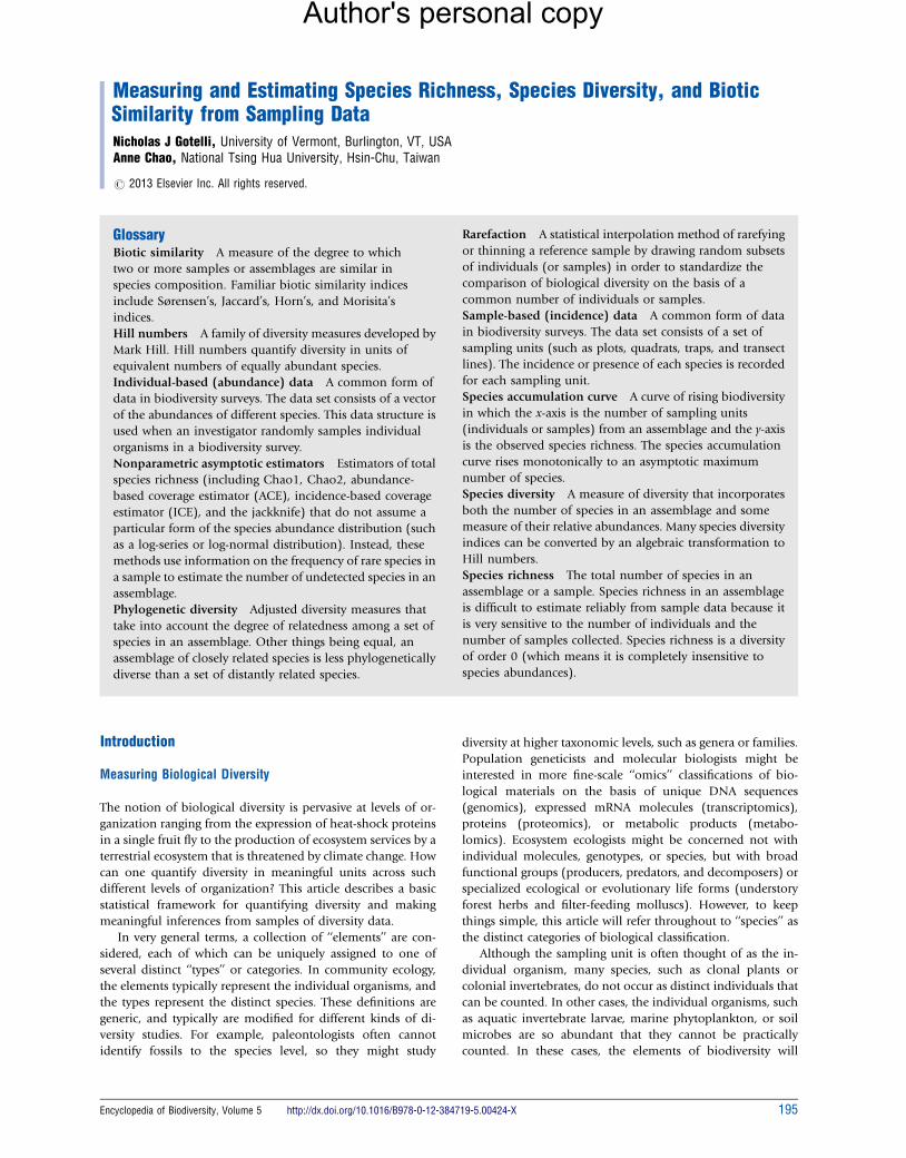
Although species richness is a key metric, it is not the only
component of species diversity. Consider two woodlands, each
with 20 species of trees. In the first woodland, the 20 species
are equally abundant, and each species comprises 5% of the
total abundance. In the second woodland, one dominant
species comprises 81% of the total abundance, and each of the
remaining 19 species contributes only 1% to the total. Al-
though both woodlands contain 20 species, a visitor to the
first woodland would encounter most of the different tree
species in a brief visit, whereas a visitor to the second wood-
land might encounter mostly the single dominant species
(Figure 1).
Thus, a comprehensive measure of species diversity should
include components of both species richness and the relative
abundances of the species that are present. Such measures are
Community A: 20 species (p1…p20 = 0.05)
Sample #1: 20 individuals, 15 species observed, 5
Sample #2: 20 individuals, 13 species observed, 7
Community B: 20 species (p1 = 0.81, p2…p20 = 0.0
Sample #1: 20 individuals, 3 species observed, 17
Sample #2: 20 individuals, 4 species observed, 16
Figure 1 Species richness sampling in a hypothetical walk through the woeach row contains 20 characters, representing the first 20 individual trees tmaximally even, with each of the 20 species comprising 5% of the total abuyielded 15 and 13 species, respectively. Community B is highly uneven, witabundance, and the remaining 19 species contributing only 1% each. In thithree and four species, respectively.
referred to in this article as ‘‘traditional’’ diversity measures.
Ecologists have used dozens of different traditional diversity
measures, all of which assume (1) individuals within a species
are equivalent, (2) all species are ‘‘equally different’’ from one
another and receive equal weighting, and (3) diversity is
measured in appropriate units (individuals, biomass, and
percentage cover are most commonly used).
Phylogenetic, Taxonomic, and Functional Diversity
As noted in the previous section the first assumption of tra-
ditional diversity metrics (individuals within a species are
equivalent) can be relaxed by changing the operational def-
inition of ‘‘species’’ to other categories of interest. The second
assumption (all species are equally different from one an-
other) ignores aspects of phylogenetic or functional diversity,
but can also be incorporated through a generalization of
traditional diversity metrics.
For example, consider two woodlands with identical tree
species richness and evenness but with no shared species. The
species in the first woodland are all closely related oaks in the
same genus (Quercus). The species in the second woodland are
a diverse mix of oaks (Quercus) and maples (Acer), as well as
more distantly related pines (Pinus). Traditional species di-
versity metrics would be identical for both woodlands, but it is
intuitive that the second woodland is more diverse (see
Figure 2 for another example).
The concept of traditional diversity can therefore be ex-
tended to consider differences among species. All else being
equal, an assemblage of phylogenetically or functionally di-
vergent species is more diverse than an assemblage of closely
related or functionally similar species. Differences among
species can be based directly on their evolutionary histories,
either in the form of taxonomic classification (referred to as
taxonomic diversity) or phylogeny (referred to as phylogenetic
species undetected
species undetected
1)
species undetected
species undetected
ods. Each different symbol represents one of 20 distinct species, andhat might be encountered in a random sample. Community A isndance. In this assemblage, the two samples of 20 individual trees
h one species (the open circle) representing 81% of the totals assemblage, the two samples of 20 individual trees yielded only

Assemblage II II II II II I I II I
Figure 2 Phylogenetic diversity in species composition. Thebranching diagram is a hypothetical phylogenetic tree. The ancestorof the entire assemblage is the ‘‘root’’ at the top, with timeprogressing toward the branch tips at the bottom. Each node(branching point) represents a speciation or divergence event, andthe 21 branch tips illustrate the 21 extant species. Extinct species orlineages are not illustrated. The five species in Assemblage Irepresent an assemblage of five closely related species (they allshare a quite recent common ancestor). The five species inAssemblage II represent an assemblage of five distantly relatedspecies (they all share a much older common ancestor). All otherthings being equal, the community of distantly related species wouldbe considered more phylogenetically diverse than the community ofclosely related species.
Measuring and Estimating Species Richness, Species Diversity, and Biotic Similarity from Sampling Data 197
Author's personal copy
diversity (PD)) or indirectly, based on their function (referred
to as functional diversity). These metrics relax the second as-
sumption discussed in the section Species Richness and Tra-
ditional Species Diversity Metrics (all species are ‘‘equally
different’’ from one another) by weighting each species by a
measure of its taxonomic classification, phylogeny, or
function.
Biotic Similarity
These concepts of species diversity apply to metrics that are
used to quantify the diversity of single assemblages. However,
the concept of diversity can also be applied to the comparison
of multiple assemblages. Suppose again that a person visits
two woodlands, both of which have 10 trees species, each
species contributing 10% to the abundance of individual trees
within the woodland. Thus, in terms of species richness and
species diversity, the two woodlands are identical. However,
the two woodlands may differ in their species composition. At
one extreme, they may have no species in common, so they are
biologically distinct, in spite of having equal species richness
and species diversity. At the other extreme, if the list of tree
species in the two woodlands is the same, they are identical in
all aspects of diversity (including taxonomic, phylogenetic,
and functional diversity). More typically, the two woodlands
might have a certain number of species found in both
woodlands and a certain number that are found in only one.
Biotic similarity quantifies the extent to which two or more
sites are similar in their species composition and relative
abundance distribution. The concept of biotic similarity is
important at large spatial scales for the designation of bio-
geographic provinces that harbor distinctive species
assemblages with both endemic and shared elements. Biotic
similarity is also a key concept underlying the measurement of
beta diversity, the turnover in species composition among a set
of sites. In an applied context, biotic similarity indices can
quantify the extent to which distinct biotas in different regions
have become homogenized through losses of endemic species
and the introduction and spread of nonnative species. Dif-
ferences among species in evolutionary histories and func-
tional trait values can also be incorporated in similarity
measures.
Bias in the Estimation of Diversity
The true species richness and relative abundances in an as-
semblage are unknown in most applications. Thus species
richness, species diversity, and biotic similarity must be esti-
mated from samples taken from the assemblage. If the sample
relative abundances are used directly in the formulas for tra-
ditional diversity and similarity measures, the maximum
likelihood estimator (MLE) of the true diversity or similarity
measure is obtained. However, the MLEs of most species di-
versity measures are biased when sample sizes are small. When
sample size is not sufficiently large to observe all species, the
unobserved species are undersampled, and – as a consequence
– the relative abundance of observed species, on average, is
overestimated.
Because biotic diversity at all levels of organization is often
high, and biodiversity sampling is usually labor intensive,
these biases are usually substantial. Even the simplest com-
parison of species richness between two samples is compli-
cated unless the number of individuals is identical in the two
samples (which it never is) or the two samples represent the
same degree of coverage (completeness) in sampling. Ignoring
the sampling effects may obscure the influence of overall
abundance or sampling intensity on species richness. Attempts
to adjust for sampling differences by algebraic rescaling (such
as dividing S by n or by sampling effort) lead to serious dis-
tortions and gross overestimates of species richness for small
samples. Thus, an important general objective in diversity
analysis is to reduce the undersampling bias and to adjust for
the effect of undersampled species on the estimation of di-
versity and similarity measures. Because sampling variation is
an inevitable component of biodiversity studies, it is equally
important to assess the variance (or standard error) of an es-
timator and provide a confidence interval that will reflect
sampling uncertainty.
The Organization of Biodiversity Sampling Data
This article introduces a common set of notation for de-
scribing biodiversity data (Colwell et al., 2012). Consider an
assemblage consisting of N� total individuals, each belonging
to one of S distinct species. Species i has Ni individuals, so thatPSi ¼ 1 Ni ¼N�. The relative frequency pi of species i is Ni/N
�,
so thatPS
i ¼ 1 pi ¼ 1. Note here that N�, S, Ni, and pi represent
the ‘‘true’’ underlying abundance, species richness, and relative
frequencies of species. These quantities are unknowns, but can
be estimated, and one can make statistical inferences by taking
198 Measuring and Estimating Species Richness, Species Diversity, and Biotic Similarity from Sampling Data
Author's personal copy
random samples of data from such an assemblage. This article
distinguishes between two sampling structures.
Individual-Based (Abundance) Data
The reference sample is a collection of n individuals, drawn at
random from the assemblage with N� total individuals. In the
reference sample, a total of Sobs species are observed, with Xi
individuals observed for species i, so thatPS
i ¼ 1 Xi ¼ n (only
species with Xi40 contributes to the sum). Thus, the data
consist of a single vector of length S, whose elements are the
observed abundances of the individual species Xi. In this
vector, there are Sobs nonzero elements.
The abundance frequency count fk is defined as the number of
species each represented by exactly k individuals in the refer-
ence sample. Thus, f1 is the number of species represented by
exactly one individual (‘‘singletons’’) in the reference sample,
and f2 is the number of species represented by exactly two
individuals (‘‘doubletons’’). In this terminology, f0 is the
number of undetected species: species that are present in the
assemblage of N� individuals and S species, but were not
detected in the reference sample of n individuals and Sobs
species. Therefore, Sobs þ f0 ¼ S.
0 500 1000 1500 2000
5
10
15
20
Number of individuals
Spe
cies
ric
hnes
s
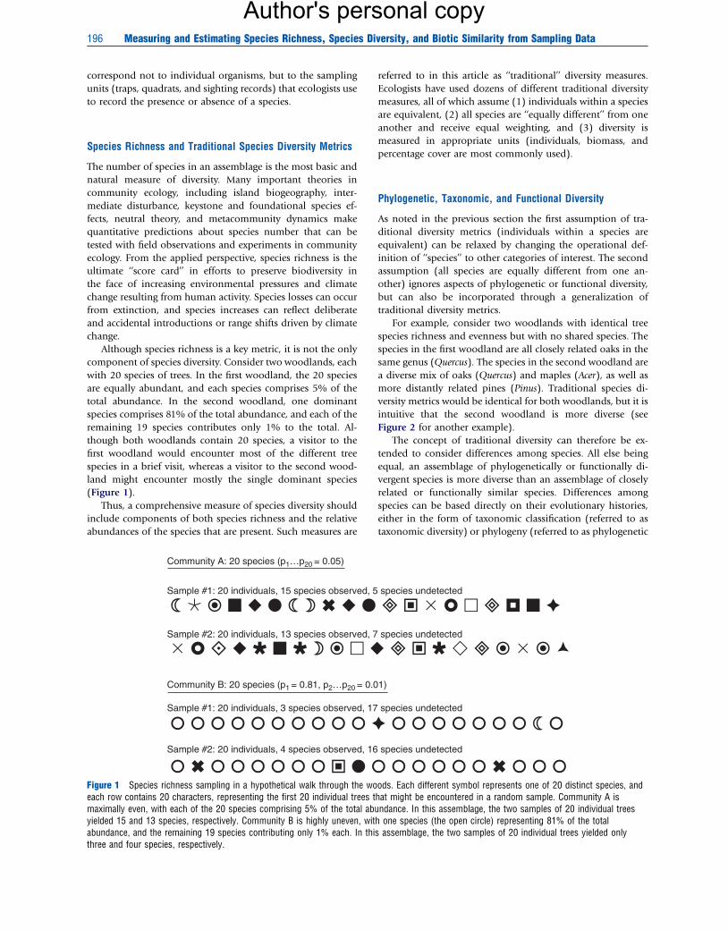
Figure 3 Species accumulation curve. The curve was generated byassuming an assemblage of 20 species whose relative abundanceswere created from a broken stick distribution (Tokeshi, 1999). The x-axis is the number of individuals sampled and the y-axis is the numberof species observed. The species accumulation curve is the smooth redline, which represents the average of 1000 random draws, samplingwith replacement, at each level of abundance. The shaded enveloperepresents a symmetric 95% bootstrap confidence interval, calculatedfrom the estimated variance of the random draws. The shape of thisspecies accumulation curve is typical: it rises rapidly at first as thecommon species are initially encountered, and then continues to risevery slowly, as much more sampling is needed to encounter all of therare species. For random samples of 500 or more individuals, it isalmost always the case that all 20 species are encountered.
Sample-Based (Incidence) Data
The reference sample for incidence data consists of a set of R
replicate sampling units (traps, plots, quadrats, search routes,
etc.). In a typical study, these sampling units are deployed
randomly in space within the area encompassing the assem-
blage. However, in a temporal study of diversity, the R sampling
units would be deployed in one place at different independent
points in time (such as an annual breeding bird census at a
single site). Within each sampling unit, the presence or absence
of each species is recorded, but abundances or counts of the
species present are not needed. The data are organized as a
species-by-sampling-unit incidence matrix, in which there are
i¼1 to S rows (species), j¼1 to R columns (sampling units),
and the matrix entry Wij¼1 if species i is detected in sampling
unit j, and Wij¼0 otherwise. If sampling is replicated in both
time and space, the data would be organized as a three-di-
mensional matrix (species� sites� times). However, most
biodiversity data sets are two dimensional, with either spatial or
temporal replication, but not both.
The row sum of the incidence matrix Yi ¼PR
j ¼ 1 Wij de-
notes the incidence-based frequency of species i for i¼1 to S.
Yi is analogous to Xi in the individual-based abundance vector.
Species present in the assemblage but not detected in any
sampling unit have Yi¼0. The total number of species ob-
served in the reference sample is Sobs (only species with Yi40
contribute to Sobs).
The incidence frequency count Qk is the number of species
each represented exactly Yi¼k times in the incidence matrix
sample, 0rkrR. For the incidence matrix,PR
k ¼ 1 kQk ¼PSi ¼ 1 Yi and Sobs ¼
PRk ¼ 1 Qk. Thus, Q1 represents the num-
ber of ‘‘unique’’ species (those that are each detected in only
one sample) and Q2 represents the number of ‘‘duplicate’’
species (those that are each detected in exactly two samples).
The zero frequency Q0 denotes the number of species among
the S species in the assemblage that were not detected in any
of the R sampling units.
Species Richness Estimation
A simple count of the number of species in a sample is usually a
biased underestimate of the true number of species, simply
because increasing the sampling effort (through counting more
individuals, examining more sampling units, or sampling a
larger area) inevitably will increase the number of species ob-
served. The effect is best illustrated in a species accumulation
curve, in which the x-axis is the number of individuals sampled
or sampling units examined and the y-axis is the number of
species observed (Figure 3). The first individual sampled always
yields one species, so the origin of an abundance-based species
accumulation curve is the point [1,1]. If the next individual
sampled is the same species, the curve stays flat with a slope of
zero. If the next individual sampled is a different species, the
curve rises to two species, with an initial slope of 1.0. Samples
from the real world fall between these two idealized extremes,
and the slope of the curve measured at any abundance level is
the probability that the next individual sampled represents a
previously unsampled species. The curve is steepest in the early
part of the collecting, as the common species in the assemblage
are detected relatively quickly. The curve continues to rise as
Measuring and Estimating Species Richness, Species Diversity, and Biotic Similarity from Sampling Data 199
Author's personal copy
more individuals are sampled, but the slope becomes shallower
because progressively more sampling is required to detect
the rare species. As long as the sampling area is sufficiently
homogeneous, all of the species will eventually be sampled and
the curve will flatten out at an asymptote that represents the
true species richness for the assemblage. For incidence data, a
similar accumulation curve can be drawn in which the x-axis
represents the number of sampling units and the y-axis is the
number of species recorded.
Interpolating Species Richness with Rarefaction
A single empirical sample of individuals or a pooled set of
sampling units represents one point on the species accumu-
lation curve, but the investigator has no way of directly de-
termining where on the curve this point lies. To compare the
richness of two different samples, they must be standardized
to a common number of individuals, for abundance samples
(Sanders, 1968; Gotelli and Colwell, 2001, 2011). Rarefaction
represents an interpolation of a biodiversity sample to a
smaller number of individuals for purposes of comparison
among samples. Typically, the abundance of the larger sample
is rarefied to the total abundance of the smaller sample to
determine if species richness (or any other biodiversity index)
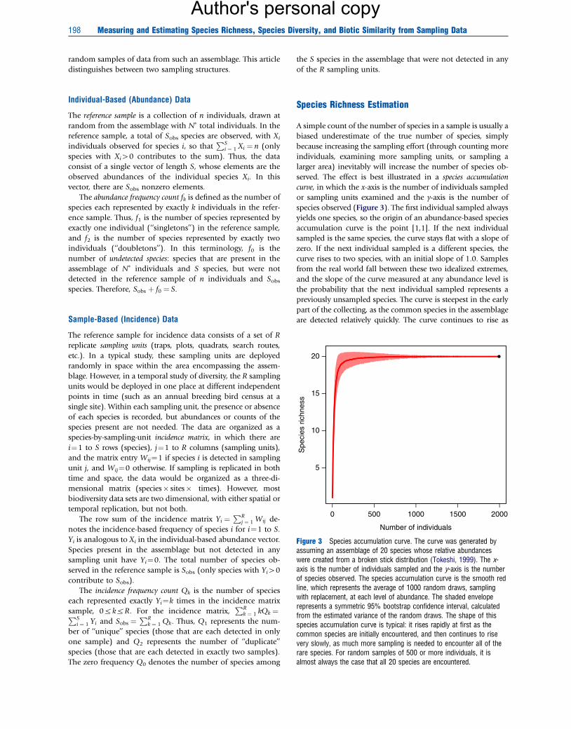
differs for a common number of individuals (Figure 4). For
incidence data, rarefaction interpolates between the reference
sample and a smaller number of sampling units.
Let Sind(m) represent the expected number of species in a
random sample of m individuals from the reference sample of
0 50 100 150 200 250
0
5
10
20
30
Number of individuals
Spe
cies
ric
hnes
s
Figure 4 Standardized comparison of species richness for twoindividual-based rarefaction curves. The data represent summarycounts of carabid beetles that were pitfall-trapped from a set of youngpine plantations (o20 years old; upper curve) and a set of old pineplantations (20–60 years old; lower curve). The solid lines are therarefaction curves, calculated from eqn [2], and the shaded polygonsare the 95% confidence intervals, calculated from the unconditionalvariance eqn [5]. The young plantation samples contained 243individuals representing 31 species, and the old plantation samplescontained 63 individuals representing nine species. The dashed anddotted vertical line illustrates a species richness comparisonstandardized to 63 individuals, which was the observed abundancein the smaller of the two data sets. Data from Niemela J, Haila Y,Halme E, et al. (1988) The distribution of carabid beetles in fragmentsof old coniferous taiga and adjacent managed forest. AnnalesZoologici Fennici 25: 107–199.
n individuals (mon). If the true probabilities (p1, p2, y, ps) of
each of the S species in the assemblage were known, and
species frequencies (X1, X2, y, XS) follow a multinomial
distribution for which the total of all frequencies is n, and cell
probabilities (p1, p2, y , pS), then
SindðmÞ ¼ S�XS
i ¼ 1
ð1� piÞm ½1�
However, the true pi values are unknown, and there is only the
reference sample with observed species abundances Xi. An
unbiased estimator for Sind(m) (Hurlbert, 1971) is
~S indðmÞ ¼ Sobs �XXi40
n� Xi
m
� �=
n
m
� �� �½2�
For incidence-based data, the corresponding equation
(Shinozaki, 1963) is
~SsampleðrÞ ¼ Sobs �XYi40
R� Yi
r
� �=
R
r
� �� �½3�
where roR is the number of sampling units in the rarefied
reference sample. The statistical model for rarefaction is sam-
pling without replacement from the reference sample.
If the area of each of the sample plots has been measured,
species richness can also be interpolated from a Coleman curve,
in which the expected species richness on an island (or sample
plot) of area a is based on a Poisson model and is a function
of the total area A of the archipelago (or the summed areas of
all the sample plots) (Coleman et al., 1982):
~SareaðaÞ ¼ Sobs �XXi40
1� a
A
� �Xi
½4�
Although the variance from the hypergeometric distribution
has traditionally been used to calculate a confidence interval
for a rarefaction curve, this variance is conditional on the
observed sample. It therefore has the undesirable property of
converging to zero when the abundance level reaches the
reference sample size. More realistically, the observed sample
is itself drawn from a much larger assemblage, so the con-
fidence intervals generally should widen as the reference
sample size is reached. This unconditional variance for
abundance data is calculated as follows (Colwell et al., 2012):
s2indðmÞ ¼
Xn
k ¼ 1
ð1� akmÞ2fk � ½~SindðmÞ�2=Sest ½5�
where Sest denotes an estimated species richness (such as
Chao1, described in the section Species Richness Estimation)
and akm ¼n� k
m
� �,n
m
� �for krn�m, akm¼0 otherwise.
The corresponding unconditional variance for incidence data
is (Colwell et al., 2004)
s2sampleðrÞ ¼
XR
k ¼ 1
ð1� bkrÞ2Qk � ½~SsampleðrÞ�2=Sest ½6�
where Sest denotes a sample-based estimated species richness
(such as Chao2, described in the section Species Richness
200 Measuring and Estimating Species Richness, Species Diversity, and Biotic Similarity from Sampling Data
Author's personal copy
Estimation) and bkr ¼R� k
r
� �,R
r
� �for krR� r, bkr¼0
otherwise. These variances allow for the calculation of 95%
confidence intervals on expected species richness for any
abundance level smaller than the observed sample (Figure 4).
Because all rarefaction curves converge at small sample
sizes toward the point [1,1] (for abundance data) or a small
number of species (for incidence data), sufficient sampling is
necessary for valid comparisons of curves. Although there are
no theoretical guidelines, empirical examples suggest that
samples of at least 20–50 individuals per sample (and pref-
erably many more) are necessary for meaningful comparisons
of abundance-based rarefaction curves.
Rarefaction curves also require comparable sampling
methods (forest samples collected from pitfall traps cannot be
validly compared to prairie samples collected from baits),
well-defined assemblages of discrete countable individuals
(for abundance-based methods), random spatial arrangement
of individuals, and random, independent sampling of
individuals (or larger sampling units for incidence-based
methods). If the spatial distribution of individuals is intras-
pecifically clumped in space, abundance-based rarefaction will
overestimate species richness, but this problem can be effect-
ively countered by increasing the spatial grain of sampling or
using incidence-based methods. Perhaps the chief disadvan-
tage of rarefaction is that point comparisons force an investi-
gator to rarefy all samples down to the smallest sample size in
the data set, so sufficient sampling is important. However,
calculation and comparison of complete rarefaction curves
and their extrapolation, with unconditional variances, help to
overcome this problem (Colwell et al., 2012).
Nonparametric Asymptotic Species Richness Estimators
Whereas rarefaction is a method for interpolating species diver-
sity data, asymptotic richness estimators are methods for ex-
trapolating species diversity out to the (presumed) asymptote,
beyond which additional sampling will not yield any new spe-
cies. Three strategies have been used to try to estimate the
asymptote of the species accumulation curve. Parametric curve
fitting uses the shape of the species accumulation curve in its
early phase to try and predict the asymptote. Asymptotic func-
tions, such as the negative exponential distribution, the Weibull
distribution, the logistic equation, and the Michaelis–Menten
equation, are fit (usually with nonlinear regression methods) to
the species accumulation data, and the asymptote can be esti-
mated as one of the parameters of this kind of model. The chief
problem is that this does not work well in comparisons with
empirical or simulated data sets, mainly because it does not
directly use information on the frequency of common and rare
species, but simply tries to forecast the shape of the rising curve.
Several different functional forms may fit the same data set
equally well, but yield drastically different estimates of the
asymptote. Because curve fitting is not based on a statistical
sampling model, the variance of the resulting asymptote cannot
be evaluated without further assumptions, and theoretical
difficulties arise for model selection.
A second strategy is to use the abundance or incidence
frequency counts (fk or Qk) and fit them to a species abundance
distribution, such as the log-series or the log-normal distri-
bution. The area under such a fitted curve is an estimate of the
total number of species present in the assemblage. The chief
weakness of these methods is that simulations show that they
work well only when the correct form of the species abun-
dance distribution is already known, but this is never the case
for empirical data. It is often not clear that existing statistical
models fit empirical data sets very well, which often depart
from expected values in the frequencies of the rare species.
Moreover, there is no guarantee that two different assemblages
follow the same kind of distribution, which complicates the
comparison of curves.
The most successful methods so far have been nonpara-
metric estimators (Colwell and Coddington, 1994), which use
the rare frequency counts to estimate the frequency of the
missing species (f0 or Q0). For incidence data, these estimators
are similar to mark-recapture models that are used in dem-
ography to estimate the total population size and are based on
statistical theorems developed by Alan Turing and I.J. Good
from cryptographic analysis of Wehrmacht coding machines
during World War II. The basic concept of their theorem is that
abundant species – which are certain to be detected in samples
– contain almost no information about the undetected spe-
cies, whereas rare species – which are likely to be either un-
detected or infrequently detected – contain almost all the
information about the undetected species.
If there are many undetectable or ‘‘invisible’’ species in a
hyperdiverse assemblage, it will be impossible to obtain a
good estimate of species richness. Therefore, an accurate lower
bound for species richness is often of more practical use than
an imprecise point estimate. Based on the concept that rare
species carry the most information about the number of un-
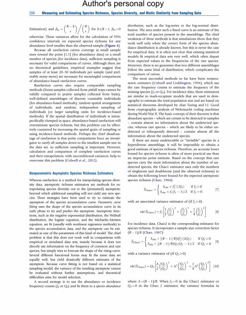
detected species, the Chao1 estimator uses only the numbers
of singletons and doubletons (and the observed richness) to
obtain the following lower bound for the expected asymptotic
species richness (Chao, 1984):
SChao1 ¼Sobs þ f 2
1 =ð2f2Þ if f240
Sobs þ f1ðf1 � 1Þ=2 if f2 ¼ 0
(½7�
with an associated variance estimator of (if f240)
varðSChao1Þ ¼ f21
2
f1f2
� �2
þ f1f2
� �3
þ 1
4
f1f2
� �4" #
½8�
For incidence data, Chao2 is the corresponding estimator for
species richness. It incorporates a sample-size correction factor
(R� 1)/R (Chao, 1987):
SChao2 ¼Sobs þ ½ðR� 1Þ=R�Q2
1=ð2Q2Þ if Q240
Sobs þ ½ðR� 1Þ=R�Q1ðQ1 � 1Þ=2 if Q2 ¼ 0
(½9�
with a variance estimator of (if Q240)
varðSChao2Þ ¼Q2A
2
Q1
Q2
� �2
þ A2 Q1
Q2
� �3
þ 1
4A2 Q1
Q2
� �4" #
½10�
where A¼(R� 1)/R. When f2¼0 in the Chao1 estimator or
Q2¼0 in the Chao 2 estimator, the variance formulas in
Measuring and Estimating Species Richness, Species Diversity, and Biotic Similarity from Sampling Data 201
Author's personal copy
eqns [9] and [10] need modification; the modified variances
are available in Chao and Shen (2010).
The Chao1 estimator may be very useful for data sets in
which it is too time consuming to count the frequencies of all
abundance classes, but it is relatively easy to count just the
number of singleton and doubleton species. Chao1 and
Chao2 are intuitive and very easy to calculate, and often per-
form just as well as more complex asymptotic estimators.
A more general approach is to use information on the
frequency of other rare species, not just singletons and dou-
bletons. A cut-off value k denotes frequencies of rare species
(frequencyrk) and abundant species (frequency4k). The
cut-off k¼10 works well with many empirical data sets.
Let the total number of observed species in the abundant
species group be Sabun ¼P
i4kfi and the number of observed
species in the rare species group be Srare ¼Pk
i ¼ 1 fi. Define
nrare ¼Pk
i ¼ 1 ifi and the coverage estimate Crare ¼ 1� f1=nrare.
Coverage is the estimated proportion of the total number of
N� individuals in the assemblage that is represented by the
species recorded in the sample. It is a reliable measure of the
degree of sample completeness. The Abundance-based Coverage
Estimator (ACE) is (Chao, 2005)
SACE ¼ Sabun þSrare
Crare
þ f1
Crare
g2rare ½11�
where g2rare is the square of the estimated coefficient of vari-
ation of the species relative abundances:
g2rare ¼max
Srare
Crare
Pki ¼ 1 iði� 1Þfi
ðSki ¼ 1ifiÞðSk
i ¼ 1ifi � 1Þ � 1,0
� ½12�
An approximate variance for the ACE can be obtained using a
standard asymptotic approach.
For incidence data, there is a corresponding Incidence-based
Coverage Estimator (ICE). As with ACE, first a cut-off point k is
selected that partitions the data into an infrequent species
group (incidence frequency not larger than k) and a frequent
species group (incidence frequency larger than k). The cut-off
k¼10 is recommended. Denote the number of species in the
frequent group by Sfreq ¼P
i4kQi and the number of species
in the infrequent group by Sinfreq ¼Pk
i ¼ 1 Qi. The estimated
sample coverage for the infrequent group is Cinfreq ¼ 1�Q1=Pki ¼ 1 iQi. Let the number of sampling units that include
at least one infrequent species be Rinfreq. Then ICE is
expressed as
SICE ¼ Sfreq þSinfreq
Cinfreq
þ Q1
Cinfreq
g2infreq ½13�
where g2infreq is the squared estimate of the coefficient of vari-
ation of the species relative incidences:
g2infreq ¼max
Sinfreq
Cinfreq
Rinfreq
Rinfreq � 1 �
(
�Pk
i ¼ 1 i i� 1ð ÞQiPki ¼ 1 iQi
� Pki ¼ 1 iQi � 1
�� 1,0
)½14�
In addition to Chao1, Chao2, ACE, and ICE, the jackknife
method provides another class of nonparametric estimators
of asymptotic species richness. Jackknife techniques were
developed as a general method to reduce the bias of a biased
estimator. Here the biased estimator is the number of species
observed in the sample. The basic idea with the jth-order
jackknife method is to consider subdata by successively de-
leting j individuals from the data. The first-order jackknife
turns out to be
Sjk1 ¼ Sobs þn� 1
nf1ESobs þ f1 ½15a�
That is, only the number of singletons is used to estimate the
number of unseen species. The second-order jackknife esti-
mator, which uses singletons and doubletons, has the fol-
lowing form:
Sjk2 ¼ Sobs þ2n� 3
nf1 �
ðn� 2Þ2
nðn� 1Þ f2ESobs þ 2f1 � f2 ½15b�
Higher-order jackknife estimators are available, although they
give increasingly less weight to the more common species
frequencies.
For replicated incidence data, the first-order jackknife for R
samples is
Sjk1 ¼ Sobs þR� 1
RQ1 ½16a�
and the second-order jackknife is
Sjk2 ¼ Sobs þ2R� 3
RQ1 �
ðR� 2Þ2
RðR� 1ÞQ2 ½16b�
All jackknife estimators can be expressed as linear combin-
ations of frequency counts, and thus approximate variances
and confidence intervals can be directly obtained.
Extrapolating Species Richness
Based on a reference sample of n individuals, the extrapolation
or prediction problem is to estimate the expected number of
species Sind(nþm�) in an augmented sample of nþm� indi-
viduals from the assemblage (m�40). Under a simple multi-
nomial model, Shen et al. (2003) derived the following useful
predictor with an asymptotic variance:
~S indðnþm�Þ ¼ Sobs þ f 0 1� 1� f1
nf 0
!m�24
35
ESobs þ f 0 1� exp �m�
n
f1
f 0
!" #½17�
where f 0 is an estimator for f0 (the number of undetected
species). It is suggested that f 0 can be obtained by using either
the Chao1 estimator ðf 0 ¼ SChao1 � SobsÞ or the ACE estimator
ðf 0 ¼ SACE � SobsÞ.The corresponding extrapolation formula and its asymp-
totic variance for the Coleman area-based Poisson sampling
model were developed by Chao and Shen (2004). An esti-
mator for the expected number of species Sarea(Aþ a�) in an
202 Measuring and Estimating Species Richness, Species Diversity, and Biotic Similarity from Sampling Data
Author's personal copy
augmented area Aþ a�(a�40) based on a reference sample of
area A is
~Sarea Aþ a�ð Þ ¼ Sobs þ f 0 1� exp � a�
A
f1
f 0
!" #½18�
where f 0 is the same as in the individual-based model.
For sample-based data with R sampling units comprising
the reference sample, Chao et al. (2009, Appendix A) de-
veloped a Bernoulli-product model and derived the following
estimator for the expected number of species Ssample(Rþ r�) in
an augmented set of Rþ r� sampling units (r�40) from the
assemblage:
~SsampleðRþ r�Þ ¼ Sobs þ Q0 1� 1� Q1
Q1 þ RQ0
� �r�" #
ESobs þ Q0 1� exp�r�Q1
Q1 þ RQ0
� �� �½19�
Here Q0, which is an estimator for Q0, can be obtained from
either the Chao2 estimator Q0 ¼ SChao2 � Sobs
�or the ICE
Q0 ¼ SICE � Sobs
�.
For each of the these models, Colwell et al. (2012) linked
the interpolation (rarefaction) curve and the corresponding
0 20,000 40,000 60,000
0
50
100
150
Accumulated # of museum records
Spe
cies
ric
hnes
s
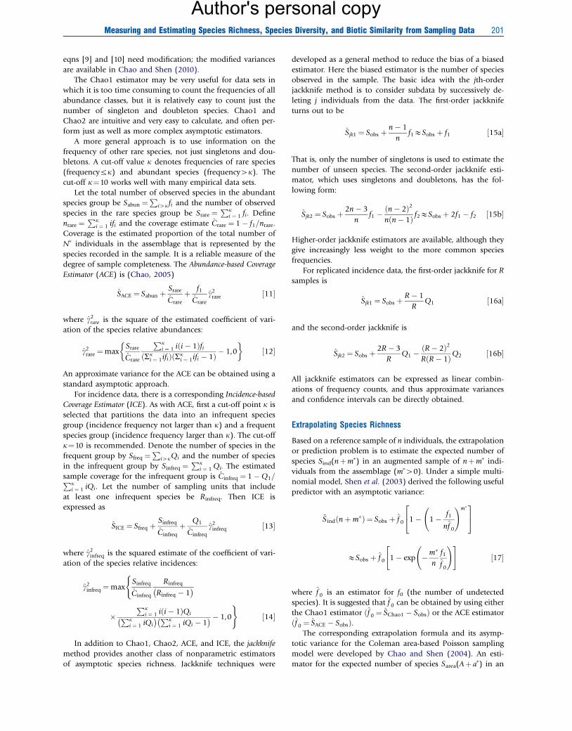
Figure 5 A smoothed rarefaction and extrapolation curve. The x-axisis the number of individual, geo-referenced, dated ant specimens inNew England, and the y-axis is the observed number of species. Thetotal collection (the reference sample, filled circle) included 127 speciesand 20,225 individual records. The solid curve is the rarefaction curveinterpolated from the reference sample. The dashed curve is theextrapolation, which extends to a minimum asymptotic estimator(Chao1) of B135 species (open diamond). This number accords wellwith an independent estimate of an additional eight species that occurin suitable habitat in New York and Quebec. These eight species arelikely to occur in New England, but so far they have not been collected.However, the extrapolation to reach the Chao1 estimator extends toover 70,000 museum records, and the confidence interval (shadedpolygon) is therefore fairly broad. The data set was compiled frommuseum records and private collections of ants sampled throughoutthe New England states of the USA (RI, CT, MA, VT, NH, and ME)between 1900 and 2011. Data modified from Ellison AM, Gotelli NJ,Farnsworth EJ, and Alpert GD (2012) A Field Guide to the Ants of NewEngland. New Haven, CT: Yale University Press.
extrapolation (prediction) curve to yield a single smooth curve
meeting at the reference sample (Figure 5). They also derived
95% (unconditional) confidence intervals for the interpolated
and extrapolated richness estimates. Thus, rigorous statistical
comparison can be performed not only for rarefaction but also
for extrapolated richness values. This link helps to avoid the
problem of discarding data and information from larger sam-
ples that is necessary for comparisons using the traditional
rarefaction method. However, the extrapolations become highly
uncertain if they are extended beyond approximately double the
reference sample size. For both individual- and sample-based
data, the additional sample size needed, beyond the reference
sample, to attain the estimated asymptotic species richness, or
to detect a specified proportion of asymptotic richness, is pro-
vided in Chao et al. (2009) and Colwell et al. (2012).
Species Diversity
Species Diversity Metrics
Although species richness is the most popular and intuitive
measure for characterizing diversity, the section Species Rich-
ness Estimation emphasizes that it is a very difficult parameter
to estimate reliably from small samples, especially for hyper-
diverse assemblages with many rare species. Species richness
also does not measure the evenness of the species abundance
distribution. Over the span of many decades, ecologists have
proposed a plethora of diversity measures that incorporate
both species richness and evenness, using both parametric and
nonparametric approaches (Magurran, 2004).
For example, parametric approaches assume a particular
species abundance distribution (such as the log-normal or
gamma) or a species rank abundance distribution (such as the
negative binomial or log series), and then estimate parameters
from the distribution model that quantify the heterogeneity
among species in their relative frequencies. However, as with
the estimation of asymptotic richness, these methods often do
not perform well unless the ‘‘true’’ species abundance distri-
bution is known, which is never the case (Colwell and Cod-
dington, 1994; Chao, 2005).
Nonparametric methods make no assumptions about the
mathematical form of the underlying species abundance dis-
tribution, and they have been widely used not only in ecology
but also in information science, economics, genetics, and
linguistics (see Jost, 2007; Jost et al., 2011; Chao and Jost, in
press; Tuomisto, this volume for reviews). The most popular
of these measures is the Shannon entropy,
HSh ¼ �XS
i ¼ 1
pi logpi ½20�
where S is the number of species in the assemblage and the ith
species relative abundance is pi. Shannon entropy quantifies
the uncertainty in the species identity of a randomly chosen
individual in the assemblage. Another measure that has been
widely used in economics and genetics, as well as in ecology, is
the Gini–Simpson index,
HGS ¼ 1�XS
i ¼ 1
p2i ½21�

Measuring and Estimating Species Richness, Species Diversity, and Biotic Similarity from Sampling Data 203
Author's personal copy
which measures the probability that two randomly chosen
individuals (selected with replacement) belong to two differ-
ent species. The measure 1�HGS ¼PS
i ¼ 1 p2i is referred to as
the Simpson index. With an adjustment for N�, the total
number of individuals in the assemblage, the Gini–Simpson
index is closely related to the ecological index PIE (Hurlbert,
1971), the probability of an interspecific encounter:
PIE¼ ½N�=ðN� � 1Þ�HGS ½22�
which measures the probability that two randomly chosen
individuals (selected without replacement) belong to two dif-
ferent species. Both PIE and the Gini–Simpson index have a
straightforward interpretation as a probability. When PIE is
applied to species abundance data, it is equivalent to the slope
of the individual-based rarefaction curve measured at its base.
However, the units of the Gini–Simpson index and PIE are
probabilities that are bounded between 0 and 1, and the units
of Shannon entropy are logarithmic units of information.
These popular complexity measures do not behave in the same
intuitive way as species richness (Jost, 2007).
The ecologist MacArthur (1965) was the first to show that
Shannon entropy (when computed using natural logarithms)
can be transformed to its exponential exp(HSh), and the
Gini–Simpson index can be transformed to 1= 1�HGSð Þ ¼1=PS
i ¼ 1 p2i , yielding two new indices that measure diversity in
units of species richness. In particular, these transformed in-
dices measure diversity in units of ‘‘effective number of spe-
cies’’ – the equivalent number of equally abundant species
that would be needed to give the same value of the diversity
measure. When all species are equally abundant, the effective
number of species is equal to the richness of the assemblage.
These converted measures, like species richness itself, sat-
isfy an important and intuitive property called the ‘‘replication
principle’’ or the ‘‘doubling property’’ (Hill, 1973): if N
equally diverse assemblages with no shared species are pooled
in equal proportions, then the diversity of the pooled assem-
blages should be N times the diversity of each single assem-
blage. Simple examples show that Shannon’s entropy and
Gini–Simpson measures do not obey the ‘‘replication prin-
ciple.’’ However the transformed values of these indices do
obey the replication principle.
Hill Numbers
The ecologist Mark Hill incorporated the transformed Shan-
non and Gini–Simpson measures, along with species richness,
into a family of diversity measures later called ‘‘Hill numbers,’’
all of which measure diversity as the effective number of
species. Different Hill numbers qD are defined by their ‘‘order’’
q as (Hill, 1973)
qD ¼XS
i ¼ 1
pqi
!1=ð1�qÞ
½23a�
This equation is undefined for q¼1, but in the limit as q tends
to 1:
1D ¼ limq-1
qD ¼ exp �XS
i ¼ 1
pi logpi
!¼ expðHshÞ ½23b�
The parameter q controls the sensitivity of the measure to
species relative abundance. When q¼0, the species relative
abundances do not count at all (no ‘‘discounting’’ for uneven
abundances), and 0D equals species richness. When q¼1, the
Hill number 1D is the exponential form of Shannon entropy,
which weighs species in proportion to their frequency and can
be roughly interpreted as the number of ‘‘typical species’’ in
the assemblage (Chao et al., 2010; Chao and Jost, in press).
When q¼2, 2D equals 1/(1�HGS), which heavily weights the
most common species in the assemblage; the contribution
from rare species is severely discounted. The measure 2D can
be roughly interpreted as the number of ‘‘very abundant
species’’ in the assemblage. Because all Hill numbers of higher
order place increasingly greater weight on the most abundant
species, they are much less sensitive to sample size (number of
individuals or plots surveyed) than the most popular Hill
numbers (q¼0, 1, 2). Hill numbers with negative exponents
can also be calculated, but they place so much weight on rare
species they have poor sampling properties.
Thus, the measure of diversity using Hill numbers can
potentially depend on the order q that is chosen. However,
because all Hill numbers need not be integers, and all have
common units of species richness, they can be portrayed on a
single graph as a function of q. This ‘‘diversity profile’’ of
effective species richness versus q portrays all of the infor-
mation about species abundance distribution of an assem-
blage (Figure 6). The diversity profile curve is a decreasing
function of q (Hill, 1973). The more uneven the distribution
of relative abundances, the more steeply the curve declines.
For a perfectly even assemblage, the profile curve is a constant
at the level of species richness.
Estimation of Hill Numbers
All of the Hill numbers (including species richness) as well as
the untransformed Gini–Simpson index and Shannon entropy
are sensitive to the number of individuals and samples col-
lected. The sample-size dependence diminishes as q increases
because the higher-order Hill numbers are more heavily
weighted by frequencies of common species, and the estimates
of those frequencies are not very sensitive to sample size. In
contrast, with increasing numbers of individuals or samples
collected, rare species continue to be added to the sample,
making richness and other low Hill numbers more sample size
dependent.
The MLE for the Gini–Simpson index, HGS,MLE ¼ 1�PSi ¼ 1 ðXi=nÞ2, is biased downward, and the bias in some cases
can be substantial. The minimum variance unbiased estimator
(MVUE) of the Gini–Simpson index has the following rela-
tionship to its MLE:
HGS,MVUE ¼ 1�XS
i ¼ 1½XiðXi � 1Þ�=½nðn� 1Þ�
¼ ½n=ðn� 1Þ�HGS,MLE ½24a�
This MVUE is equivalent to the estimator of PIE and is
relatively invariant to sample size. Thus, a nearly unbiased
estimator for Hill number of order 2 is
2D ¼ 1=XS
i ¼ 1½XiðXi � 1Þ�=½nðn� 1Þ� ½24b�

0 1 2 3 4 5
0
20
40
60
80
100
120
Order q
Hill
num
ber
Completely even
Slightly uneven
Moderately uneven
Highly uneven
Figure 6 Diversity profile for assemblages of differing evenness.The x-axis is the order q in the Hill number (eqn [23a]), and isillustrated for values of q from 0 to 5. The y-axis is the calculatedHill number (the equivalent number of equally abundant species).Each of the four assemblages has exactly 100 species and 500individuals, but they differ in their relative evenness: (1) completelyeven assemblage (black solid line): each species is represented byfive individuals; (2) slightly uneven assemblage (red dashed line): 50species each represented by seven individuals and 50 species eachrepresented by three individuals (this structure is denoted as {50� 7,50� 3}); (3) moderately uneven assemblage (green dotted line):{22� 10, 28� 5, 40� 3, 10� 2}; (4) highly uneven assemblage (bluedash–dot line): {1� 120, 1� 80, 1� 70, 1� 50, 3� 20, 3� 10,90� 1}. For q¼0, the Hill number is species richness, which is equalto 100 for all assemblages. Because Hill numbers represent theequivalent number of equally abundant species, the curve for theperfectly even assemblage (black solid line) does not change as q isincreased. Larger values of q place progressively more weight oncommon species, so the equivalent number of equally abundantspecies is much lower for the more uneven assemblages than formore even assemblages.
204 Measuring and Estimating Species Richness, Species Diversity, and Biotic Similarity from Sampling Data
Author's personal copy
For an integer qZ2, a similar derivation leads to a nearly
unbiased estimator for qD.
qD ¼XS
i ¼ 1½XiðXi � 1Þ?ðXi � qþ 1Þ�
n
=½nðn� 1Þ?ðn� qþ 1Þ�o1=ð1�qÞ
½24c�
These estimators for qZ2 are almost independent of sample
size, because all the higher-order Hill numbers are mainly
dominated by the number of very abundant species. The es-
timated diversity profile curve is thus generally slowly varying
for qZ2.
The estimation of entropy has been well studied in infor-
mation science, physics, and statistics. Unfortunately, an un-
biased estimator for Shannon entropy does not exist for any
fixed sample size of n. As noted earlier, using Xi/n as a simple
estimator of the true pi value yields the MLE of entropy, which
is negatively biased. An estimator of Shannon entropy with
low bias is the following Horvitz–Thompson-type estimator
(Chao and Shen, 2003):
HSh ¼ �XS
i ¼ 1
~pi logð~piÞ1� ð1� ~piÞ
n ½25a�
where ~pi ¼ ðXi=nÞð1� f1=nÞ is an estimator of the true pi. Only
the detected species contribute to the summation because~pi ¼ 0 for any undetected species. The denominator 1�ð1� ~piÞ
n is the estimated probability that the ith species is
detected in the sample, and the inverse of this probability is
used as a weight for the ith species. Thus, the larger the
probability of detection, the smaller the weight in the Horvitz-
Thompson estimator. The weights adjust the estimator to
compensate for missing species. For q¼1, a low-bias estimator
of the Hill number is
1D ¼ exp �XS
i ¼ 1
~pi logð~piÞ1� ð1� ~piÞ
n
!½25b�
In summary, the statistical properties of Hill numbers de-
pend on the order q. Equation [24b] is a nearly unbiased
estimator of diversity for q¼2, and eqn [25b] is a low-bias
estimator for q¼1. As discussed in the section Species richness
estimation, total species richness (0D¼S) is much more dif-
ficult to estimate because it is very sensitive to rare species that
are often undetected, even in relatively large samples. Several
nonparametric species richness estimators that can be used for
estimating 0D are provided in the section Nonparametric
Asymptotic Species Richness Estimators. Then an estimated
diversity profile can be constructed by plotting fqD; q¼0,1,2,3,yg with respect to q, based on estimators given in
eqns [24b], [24c], and [25b]. The variance of each estimator in
the profile can be approximated by a standard asymptotic
method, and a 95% confidence interval can thus be con-
structed as the estimator71.96 s.e. for each value of q, if the
sample size is sufficiently large.
Taxonomic and PD
To quantify taxonomic or PD, species are placed on a
branching tree (a cladogram) that describes their evolutionary
relationships (Figure 2). The base of the tree represents the
ancestral taxon, the branching forks (nodes) represent speci-
ation or divergence events, the branch tips represent the
contemporary species (not all of which may be represented in
any particular assemblage), and time is measured in the ver-
tical axis, increasing from the base of the tree to the branch
tips. (For paleontological applications, the tips may be extinct
lineages.) All other things being equal, an assemblage in
which all the species are closely related and concentrated in
one region of the tree should be less diverse than an assem-
blage in which the same number of species is widely distrib-
uted among distant branch tips of the tree.
This article distinguishes two types of phylogenetic trees:
ultrametric and nonultrametric trees. A tree is called ultra-
metric if all branch tips are the same distance from the basal
node. For example, if the branch lengths are proportional to
divergence time, the tree is ultrametric. A Linnean taxonomic
tree, in which species are simply classified into a taxonomic
hierarchy (Kingdom, Phylum, Class, Order, Family, Genus, and

p1+p2+p3
t = 4.5L5
t = 3
L1
L4T
Tim
e
t = 0
p2+p3t = 0.5L2 L3
(Present time) p1 p2 p3
Figure 7 Calculation of mean phylogenetic diversity and branchdiversity. In this hypothetical rooted phylogenetic tree, the ancestorto the assemblage is depicted at the top, and there are three extantspecies living at the present, depicted at the bottom, with relativeabundances (p1, p2, p3) ¼ (0.2, 0.3, 0.5). The tree is ultrametric, sothe total branch length from the ancestor to any descendant speciesin the present is the same. To evaluate the phylogenetic diversity atthe time T ¼ 5 time steps in the past, we first create the set BT
which includes five branches with lengths (L1, L2, L3, L4, L5) ¼ (4,1, 1, 3, 1) and the corresponding abundances (a1, a2, a3, a4, a5) ¼(p1, p2, p3, p2þ p3, p1þ p2þ p3). We next measure the lineagediversity qD(t) at any time steps 0 o t o T. We use three different‘‘sampling times’’ as examples; these three sampling timescorrespond to the three distinct assemblages that would berepresented by diversity sampling at three points in the past. For thefirst sampling time, t¼0.5, lineage diversity qD(t ) is measured as theHill numbers for three lineages (species) with relative abundances(p1, p2, p3); for the second sampling time t¼3, lineage diversityqD(t ) is measured as the Hill numbers for two lineages (species)with relative abundances (p1, p2þ p3); for the third sampling timet¼4.5, lineage diversity qD(t ) is measured as the Hill numbers foronly one lineage (species) with relative abundance p1þ p2þ p3¼1.The average of these Hill numbers qD(t ) over the interval [� T, 0]gives the mean phylogenetic diversity qD ðT Þ of order q over T timesteps. The branch diversity is qPD(T)¼T � qD ðT Þ: These twodiversities can be calculated for any fixed TZ0; their pattern as afunction of T is plotted in Figure 8. (For example, if T is changed tothe tree height T�¼4 (distance between tree base and tips), then thebranch set includes four branches (L1, L2, L3, L4)¼(4, 1, 1, 3) withthe corresponding abundances (a1, a2, a3, a4)¼(p1, p2, p3, p2þ p3),and the lineage diversity is averaged over [� 4, 0] to obtain qD ðT�Þand qPD(T �)¼T� � qD ðT�Þ:)
Measuring and Estimating Species Richness, Species Diversity, and Biotic Similarity from Sampling Data 205
Author's personal copy
Species), can be regarded as a special case of an ultrametric
tree. In contrast, if the branch lengths are proportional to the
number of base-pair changes in a given gene, or some other
measure of genetic or morphological change, some branch tips
may be farther in absolute time from the basal node than other
branch tips, and such trees are nonultrametric.
Pielou (1975) was the first to notice that the concept of
diversity could be broadened to consider differences among
species. The earliest taxonomic diversity measure is the cladistic
diversity (CD), which is defined as the total number of taxa or
nodes in a taxonomic tree that encompasses all of the species
in the assemblage (Vane-Wright et al., 1991). Another pion-
eering work is Faith’s (1992) PD, which is defined as the sum
of the branch lengths of a phylogeny connecting all species in
the target assemblage. In both CD and PD, species abundances
are not considered.
C.R. Rao’s quadratic entropy was the first diversity measure
that accounted for both phylogeny and species abundances
(Rao, 1982). It is a generalization of the Gini–Simpson index:
QRao ¼X
i,j
dijpipj ½26a�
where dij denotes the phylogenetic distance between species i
and j, and pi and pj denote the relative abundance of species i
and j. This index measures the average phylogenetic distance
between any two individuals randomly selected from the as-
semblage. For the special case of no phylogenetic structure (all
species are equally related to one another), dii¼0 and dij¼1
(ia j), and QRao reduces to the Gini–Simpson index.
The phylogenetic entropy Hp is defined as a generalization of
Shannon’s entropy to incorporate phylogenetic distances
among species (Allen et al., 2009):
HP ¼ �X
i
Liai logai ½26b�
where the summation is over all branches, Li is the length of
branch i, and ai denotes the summed abundance of all species
descended from branch i. The notation a (abundance) here is
not the same as that (for area) in eqn [4].
The replication principle can be generalized to phylo-
genetic or functional diversity: When N completely distinct
trees (no shared nodes during the fixed time interval of
interest) with equal diversities are combined, the diversity of
the combined tree is N times the diversity of any individual
tree. Simple examples can show that neither QRao nor Hp
satisfies this replication principle. As with traditional diversity
measures, QRao and Hp can be transformed into measures that
do obey the replication principle. In an ultrametric tree with
tree height T� (the time interval between the tree base and
tips), the transformed measures are, respectively, exp(Hp/T�)
and 1/[1� (QRao/T�)].
For ultrametric trees, in addition to the order q, a time
parameter T is required to generalize Hill numbers to measure
PD in an interval from � T time steps to the present time. The
generalized phylogenetic metric is a time-averaged measure of
lineage diversity (Hill numbers) at any moment t over the time
interval [� T, 0]. The lineage diversity qD(t) at any moment t is
measured by taking a ‘‘cross-section’’ and finding the lineages
that are intersected (Figure 7). The relative abundance of each
lineage is defined as the sum of the relative abundances of all
of the descendants of that lineage in the present-day assem-
blage. Thus, qD(t) can be quantified by a Hill number. The
average of these Hill numbers qD(t) over the interval [� T, 0]
gives the mean PD of order q over T time steps (Chao et al.,
2010):
qDðTÞ ¼XiABT
Li
Ta
qi
( )1=ð1�qÞ
½27�
where BT denotes the set of all branches in the time interval
[� T, 0], Li is the length (duration) of branch i in the set BT,
and ai is the total abundance of extant species descending
from branch i; see Figure 7 for a hypothetic ultrametric tree.

206 Measuring and Estimating Species Richness, Species Diversity, and Biotic Similarity from Sampling Data
Author's personal copy
This measure qDðTÞ gives the mean effective number of
maximally distinct lineages (or species) T time steps in the
past. The diversity of a tree with qD ðTÞ¼z in the time period
[� T, 0] is the same as the diversity of an assemblage con-
sisting of z equally abundant and maximally distinct species
with all branch lengths T.
The branch diversity or phylogenetic diversity qPD(T) of
order q through T time steps before present is defined as the
product of qD ðTÞ and T . The measure qPD(T) given below
quantifies ‘‘the total effective number of lineage-lengths or
lineage-time steps’’ (Chao et al., 2010)
qPD Tð Þ ¼ T � qDðTÞ ¼XiABT
Liai
T
� �q( )1=ð1�qÞ
½28�
If q¼0 and T¼T� (tree height), then 0PD(T) reduces to Faith’s
PD. It also reduces to CD in a taxonomic tree if the branching
10
q = 0
q = 1
q = 2
2
4
6
8
Bra
nch
dive
rsity
PD
(T)
543210
0
Number of time steps T
7
8
10
9
6
Bra
nch
dive
rsity
PD
(T)
T = 4
T = 5
20 1 3 4 5
5
Order q
Figure 8 Branch diversity profile and mean phylogenetic diversity profile.phylogenetic diversity (upper right panel) as a function of the number of timstructure of the phylogenetic tree in Figure 7, assuming (p1, p2, p3)¼(0.2,profile of qPD(T) (lower left panel) as a function of order q for T¼4 (tree h(lower right panel) as a function of order q for T¼0, 4, and 5, assuming (pbranch diversity for T¼0 is 0 as all branch lengths are 0. The mean phylogp3)¼(0.2, 0.3, 0.5).
of each Linnaean taxonomic category is assigned a time step of
unit length. A PD profile can be constructed by plotting bothqPD(T) and qD ðTÞ as a function of T for q¼0, 1, and 2. It is
also informative to construct another diversity profile by
plotting qPD(T) and qD ðTÞ as a function of order q for some
selected values of temporal perspective T. See Figure 8 for a
numerical example. In most applications, ecologists are
interested in the case T¼T� (tree height) or the divergence
time between the species group of interest and its nearest
outgroup. The divergence time of the most recent common
ancestor of all extant taxa is another useful comparison.
For nonultrametric trees, the time parameter T is general-
ized to T, where T ¼P
iABTLiai represents the abundance-
weighted mean base change per species and BT denote the set
of branches connecting all focal species. The diversity of a
nonultrametric tree with mean evolutionary change T is the
same as that of an ultrametric tree with a time step T.
q = 0
q = 1
Mea
n ph
ylog
enet
ic d
iver
sity
q = 2
543210
Number of time steps T
1.0
1.5
2.0
2.5
3.0
3.5
T = 0
2.0
2.5
3.0
1.5
Mea
n ph
ylog
enet
ic d
iver
sity
T = 5
T = 4
2 3 4 5
1.0
Order q
0 1
(a) Branch diversity profile of qPD(T) (upper left panel) and meane steps (T) in the past (0oTo5) for q¼0, 1, and 2, based on the
0.3, 0.5) and (L1, L2, L3, L4, L5)¼(4, 1, 1, 3, 1). (b) Branch diversityeight) and T¼5 time steps, and mean phylogenetic diversity profile of
1, p2, p3)¼(0.2, 0.3, 0.5) and (L1, L2, L3, L4, L5)¼(4, 1, 1, 3, 1). Theenetic diversity for T¼0 are the traditional Hill numbers for (p1, p2,
Measuring and Estimating Species Richness, Species Diversity, and Biotic Similarity from Sampling Data 207
Author's personal copy
Therefore, the diversity formula for a nonultrametric tree is
obtained by replacing T in the qD ðTÞ and qPD(T) with T.
Equation [27] can also describe taxonomic diversity, if the
phylogenetic tree is a Linnaean tree with L levels (ranks), and
each branch is assigned unit length. It also describes func-
tional diversity, if a dendrogram can be constructed from a
trait-based distance matrix using a clustering scheme (Petchey
and Gaston, 2002). Thus, Hill numbers can be effectively
generalized to incorporate taxonomy, phylogeny, and function
and provide a unified framework for measuring biodiversity
(Chao and Jost, in press).
Estimation of phylogenetic and functional diversity from
small samples has not been well studied. As with the estima-
tion of simple Hill numbers, phylogenetic diversity qD ðTÞ andqPD(T) can be accurately estimated only for q¼2. Like the
Gini–Simpson index, the MVUE of Rao’s quadratic entropy
exists under a multinomial model:
QMVUE ¼X
i,j
dijXiXj=½nðn� 1Þ� ½29�
Thus, 2D ðTÞ and 2PD(T) can be estimated by a nearly un-
biased measure using this estimator based on the transfor-
mation 2D ðTÞ¼1/[1� (QRao/T)]. With sufficient sampling,
these estimators of PD of order q¼2 are almost independent
of sample size. Further research is needed for the development
of accurate estimators of PD measures with q¼1 and 0.
Biotic Similarity
Incidence-Based Similarity Indices
The earliest published incidence-based measure of relative
compositional similarity is the classic Jaccard index from
1900. A number of incidence-based similarity measures have
been proposed since then (see Jost et al., 2011, for a review).
The Jaccard index and the Sørensen index (proposed in 1948)
are the most widely used ones, and both were originally de-
veloped to compare the similarity of two assemblages. Let S1
be the number of species in Assemblage 1, S2 be the number
of species in Assemblage 2, and S12 be the number of shared
species. The Jaccard similarity index¼S12/(S1þ S2� S12) and
the Sørensen similarity index¼2S12/(S1þ S2). A rearrange-
ment of the Sorensen index¼1/[0.5(S12/S1)�1þ0.5(S12/
S2)�1] reveals that it is the harmonic mean of two proportions:
S12/S1 (the proportion of the species in the first assemblage
that are shared with the second) and S12/S2 (the proportion of
the species in the second assemblage that are shared with the
first). The Jaccard index compares the number of shared spe-
cies to the total number of species in the combined assem-
blages, whereas the Sørensen index compares the number of
shared species to the mean number of species in a single as-
semblage. The Jaccard index is thus a comparison based on
total diversity, whereas the Sørensen index is a comparison
based on local diversity.
When one assemblage is much richer than the other, both
Sørensen and Jaccard indices become very small. Although the
low similarity value reflects the true difference between the
two assemblages, in some applications it can be more in-
formative to normalize a similarity measure so that maximum
overlap¼1.0. Lennon et al. (2001) proposed such a modifi-
cation to the Sørensen index, and it takes the form S12/min(S1,
S2); see Jost et al. (2011) for details and comparisons.
When more than two assemblages are compared, a typical
approach is to use the average of all pairwise similarities as a
measure of global similarity. However, the pairwise similarities
calculated from data tend to be correlated and are not in-
dependent. Most importantly, pairwise similarities cannot
fully characterize multiple-assemblage similarity when some
species are shared across two, three, or more assemblages
(Chao et al., 2008). It is easy to construct numerical examples
in which all pairwise similarities are identical in two sets of
assemblages, but the global similarities for the two sets are
different.
The two-assemblage incidence-based Jaccard and Sørensen
indices have been extended to multiple assemblages. Assume
that there are N assemblages and there are Sj species in the jth
assemblage and S species in the combined assemblage. Let S
denote the average number of species per assemblage. The
multiple-assemblage Jaccard similarity index¼ðS=S� 1=NÞ=ð1� 1=NÞ. The multiple-assemblage Sørensen similarity
index¼ðN � S=SÞ=ðN � 1Þ. When N¼2, these two measures
reduce to their classical two-assemblage measures. These two
measures are decreasing functions of Whittaker’s beta diversity
for species richness, which is S=S. When N assemblages are
identical, beta diversity (q¼0) is S=S¼1, and thus both Jac-
card and Sørensen similarity indices¼1. When N assemblages
are completely distinct (no shared species), beta diversity
(q¼0) is S=S¼N, and thus both Jaccard and Sørensen simi-
larity indices¼0.
These incidence-based similarity indices are widely used in
ecology and biogeography because of their simplicity and easy
interpretation. In most ecological studies, these indices are
estimated from observed richness in sample data. The re-
sulting estimates are generally biased downward, and the bias
increases when sample sizes are small or species richness is
large. They could become biased upward when shared species
are common and endemic species are very rare (Chao et al.,
2005, p. 149). The classic pairwise Jaccard and Sorensen
similarity indices calculated from sample data generally
underestimate the true similarity mainly because they do not
account for shared species at both sites that were not detected.
One strategy could be to use asymptotic species richness es-
timators (see Species Richness Estimation) to estimate species
richness in each assemblage and also to estimate species
richness in the combined assemblage, and then substitute the
estimated values into the similarity formulas. However, this
strategy inevitably inflates the variance and often renders the
resulting estimate useless. A major statistical concern is that,
based on incidence data alone, bias correction and measure-
ments of variances are impossible. Consequently, the inter-
pretation of any incidence-based index based on sample
values or estimated values becomes difficult or misleading for
comparing two (or more) highly diverse assemblages based on
limited data. Only with abundance data can one correct for
undersampling bias, as explained in the next section.
Classical incidence-based similarity indices treat abundant
and rare species equally, which oversimplifies the relation-
ships between assemblages. If species abundances can be
measured, they should be used for a more accurate
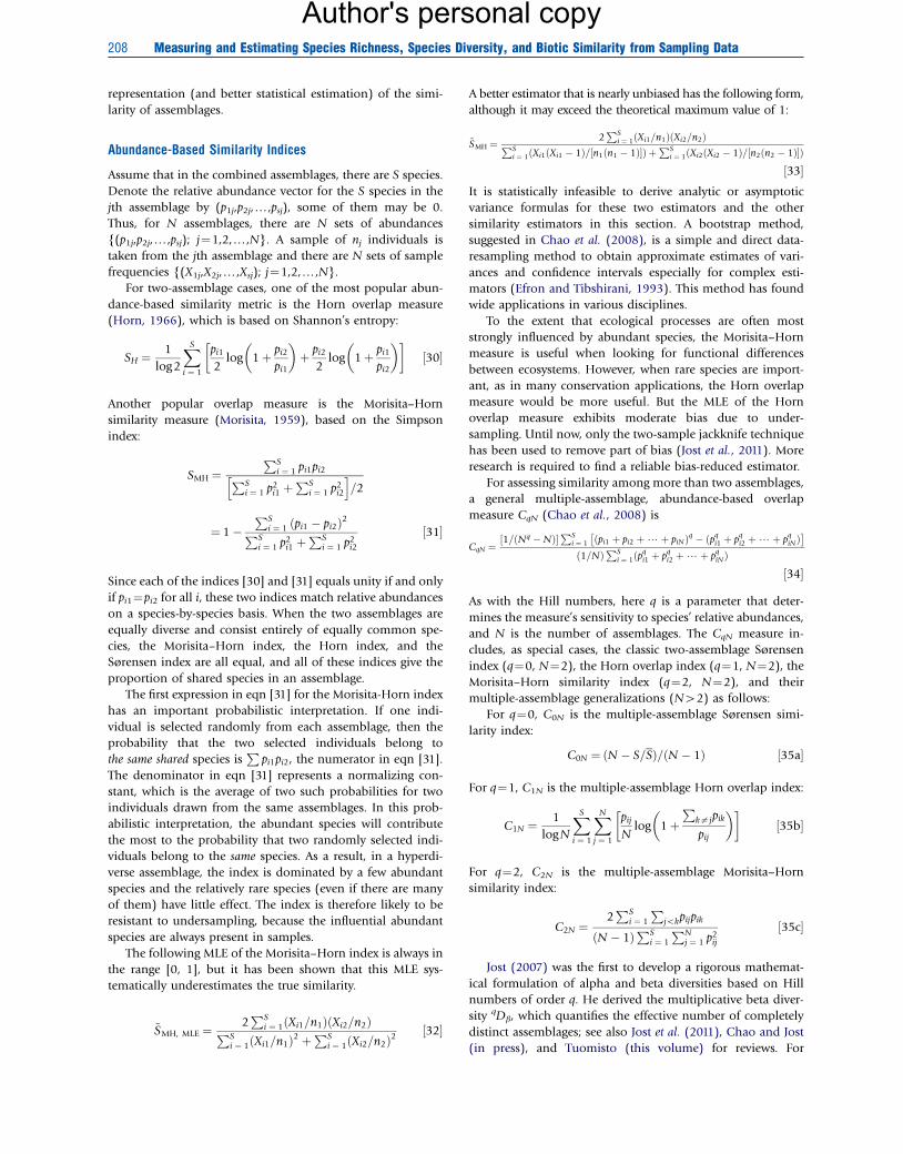
208 Measuring and Estimating Species Richness, Species Diversity, and Biotic Similarity from Sampling Data
Author's personal copy
representation (and better statistical estimation) of the simi-
larity of assemblages.
Abundance-Based Similarity Indices
Assume that in the combined assemblages, there are S species.
Denote the relative abundance vector for the S species in the
jth assemblage by (p1j,p2j,y,psj), some of them may be 0.
Thus, for N assemblages, there are N sets of abundances
{(p1j,p2j,y,psj); j¼1,2,y,N}. A sample of nj individuals is
taken from the jth assemblage and there are N sets of sample
frequencies {(X1j,X2j,y,Xsj); j¼1,2,y,N}.
For two-assemblage cases, one of the most popular abun-
dance-based similarity metric is the Horn overlap measure
(Horn, 1966), which is based on Shannon’s entropy:
SH ¼1
log2
XS
i ¼ 1
pi1
2log 1þ pi2
pi1
� �þ pi2
2log 1þ pi1
pi2
� �� �½30�
Another popular overlap measure is the Morisita–Horn
similarity measure (Morisita, 1959), based on the Simpson
index:
SMH ¼PS
i ¼ 1 pi1pi2PSi ¼ 1 p2
i1 þPS
i ¼ 1 p2i2
h i=2
¼ 1�PS
i ¼ 1 ðpi1 � pi2Þ2PSi ¼ 1 p2
i1 þPS
i ¼ 1 p2i2
½31�
Since each of the indices [30] and [31] equals unity if and only
if pi1¼pi2 for all i, these two indices match relative abundances
on a species-by-species basis. When the two assemblages are
equally diverse and consist entirely of equally common spe-
cies, the Morisita–Horn index, the Horn index, and the
Sørensen index are all equal, and all of these indices give the
proportion of shared species in an assemblage.
The first expression in eqn [31] for the Morisita-Horn index
has an important probabilistic interpretation. If one indi-
vidual is selected randomly from each assemblage, then the
probability that the two selected individuals belong to
the same shared species isP
pi1pi2, the numerator in eqn [31].
The denominator in eqn [31] represents a normalizing con-
stant, which is the average of two such probabilities for two
individuals drawn from the same assemblages. In this prob-
abilistic interpretation, the abundant species will contribute
the most to the probability that two randomly selected indi-
viduals belong to the same species. As a result, in a hyperdi-
verse assemblage, the index is dominated by a few abundant
species and the relatively rare species (even if there are many
of them) have little effect. The index is therefore likely to be
resistant to undersampling, because the influential abundant
species are always present in samples.
The following MLE of the Morisita–Horn index is always in
the range [0, 1], but it has been shown that this MLE sys-
tematically underestimates the true similarity.
~SMH, MLE ¼2PS
i ¼ 1ðXi1=n1ÞðXi2=n2ÞPSi ¼ 1ðXi1=n1Þ2 þ
PSi ¼ 1ðXi2=n2Þ2
½32�
A better estimator that is nearly unbiased has the following form,
although it may exceed the theoretical maximum value of 1:
~SMH ¼2PS
i ¼ 1ðXi1=n1ÞðXi2=n2ÞPSi ¼ 1ðXi1ðXi1 � 1Þ=½n1ðn1 � 1Þ�Þ þ
PSi ¼ 1ðXi2ðXi2 � 1Þ=½n2ðn2 � 1Þ�Þ
½33�It is statistically infeasible to derive analytic or asymptotic
variance formulas for these two estimators and the other
similarity estimators in this section. A bootstrap method,
suggested in Chao et al. (2008), is a simple and direct data-
resampling method to obtain approximate estimates of vari-
ances and confidence intervals especially for complex esti-
mators (Efron and Tibshirani, 1993). This method has found
wide applications in various disciplines.
To the extent that ecological processes are often most
strongly influenced by abundant species, the Morisita–Horn
measure is useful when looking for functional differences
between ecosystems. However, when rare species are import-
ant, as in many conservation applications, the Horn overlap
measure would be more useful. But the MLE of the Horn
overlap measure exhibits moderate bias due to under-
sampling. Until now, only the two-sample jackknife technique
has been used to remove part of bias (Jost et al., 2011). More
research is required to find a reliable bias-reduced estimator.
For assessing similarity among more than two assemblages,
a general multiple-assemblage, abundance-based overlap
measure CqN (Chao et al., 2008) is
CqN ¼½1=ðNq �NÞ�
PSi ¼ 1 ðpi1 þ pi2 þ?þ piNÞq � ðpq
i1 þ pqi2 þ?þ p
qiNÞ
� ð1=NÞ
PSi ¼ 1ðp
qi1 þ p
qi2 þ?þ p
qiNÞ
½34�
As with the Hill numbers, here q is a parameter that deter-
mines the measure’s sensitivity to species’ relative abundances,
and N is the number of assemblages. The CqN measure in-
cludes, as special cases, the classic two-assemblage Sørensen
index (q¼0, N¼2), the Horn overlap index (q¼1, N¼2), the
Morisita–Horn similarity index (q¼2, N¼2), and their
multiple-assemblage generalizations (N42) as follows:
For q¼0, C0N is the multiple-assemblage Sørensen simi-
larity index:
C0N ¼ ðN � S=SÞ=ðN � 1Þ ½35a�
For q¼1, C1N is the multiple-assemblage Horn overlap index:
C1N ¼1
logN
XS
i ¼ 1
XNj ¼ 1
pij
Nlog 1þ
Pka jpik
pij
� �� �½35b�
For q¼2, C2N is the multiple-assemblage Morisita–Horn
similarity index:
C2N ¼2PS
i ¼ 1
Pjokpijpik
ðN � 1ÞPS
i ¼ 1
PNj ¼ 1 p2
ij
½35c�
Jost (2007) was the first to develop a rigorous mathemat-
ical formulation of alpha and beta diversities based on Hill
numbers of order q. He derived the multiplicative beta diver-
sity qDb, which quantifies the effective number of completely
distinct assemblages; see also Jost et al. (2011), Chao and Jost
(in press), and Tuomisto (this volume) for reviews. For

Measuring and Estimating Species Richness, Species Diversity, and Biotic Similarity from Sampling Data 209
Author's personal copy
equally weighted assemblages, beta diversity qDb ranges be-
tween a minimum of 1 (when all assemblages are identical)
and a maximum of N, the number of assemblages in each
region (when all assemblages are completely distinct; i.e.,
there are no shared species). For example, a set of completely
distinct sites in a region of three sites attains the maximum
value of 3, whereas another set of completely distinct sites in a
region of 10 sites attains the maximum value of 10. Because
the maximum depends on the number of assemblages in the
region, beta diversities usually cannot be compared directly
among multiple regions. Instead, beta diversity should be
compared with sample-based rarefaction to a common num-
ber of samples or to a common degree of completeness of
samples in each region. However, beta diversity can be trans-
formed to the CqN measure in the range [0, 1] by the following
nonlinear transform for N equally weighted assemblages:
CqN ¼ ½ð1=qDbÞq�1 � ð1=NÞq�1�=½1� ð1=NÞq�1� ½36�
The transformed measure CqN is unity (when all assemblages
are identical) and 0 (when all assemblages are completely
distinct).
This nonlinear transformation ensures that CqN preserves
an essential property of an overlap index: The transformed
index CqN gives the true overlap A/S for all orders of q if N
assemblages each have S equally common species, exactly A
species are shared by all of them, and the remaining species
0.0
0.2
0.4
0.6
0.8
1.0
Order q
Sim
ilarit
y C
qN
0 1 2
Shared species areabundant
All species are equally abundant
Shared species are rare
Figure 9 The two-assemblage similarity profile CqN for q¼0, 1, 2.Case I: In each of Assemblages 1 and 2, there are 20 equallyabundant species, and eight species are shared. Thus, for all ordersof q, the similarity measure CqN equals the percentage of overlap ineach assemblage. That is, CqN¼8/20¼40% for all q (black solidline).Case II: In each of Assemblages 1 and 2, there are 20 species, andthe relative abundances in each assemblage are pipK/i for i¼1, 2,y, 20, where K is a normalizing constant such that the total relativeabundances is 1. Assume that the shared species are the mostabundant eight species. The similarity measure CqN increases asorder q is increased (red dashed line).Case III: Same as in Case II, but the shared species are the raresteight species. The similarity measure CqN decreases as order q isincreased (blue dotted line).
are not shared by any assemblages. No linear transformation
of beta diversity can achieve this property. See Figure 9, Case I,
for an example. The measure CqN thus quantifies the effective
average overlap per assemblage, i.e., average percentage of over-
lapped species (species that are shared by all assemblages, as
defined in the above sense) in an assemblage. Because this
measure is in a sense of ‘‘average’’ overlap, it can be compared
across regions with different number of assemblages. See Chao
et al. (2008) for more details on the interpretation of CqN
based on a simple reference set of assemblages.
Just as diversity profiles are used to characterize traditional
diversity (Figure 6) and PD (Figure 8), Chao et al. (2008)
suggest the use of a similarity profile {CqN; q¼0, 1, 2,y,N} to
describe similarity across N assemblages. It is recommended
that investigators calculate at least C0N, C1N, and C2N; see Jost
et al. (2011, p. 81) and Figure 9 for examples.
Because the overlap measure CqN is constructed from Hill
numbers of order q, the magnitude of the undersampling bias
depends on the order q. As with Hill numbers, there exists a
nearly unbiased estimator only for q¼2:
C2N ¼2PS
i ¼ 1
PjokðXij=njÞðXik=nkÞ
ðN � 1ÞPS
i ¼ 1
PNj ¼ 1½XijðXij � 1Þ=njðnj � 1Þ�
½37�
This measure quantifies the similarity of relative frequencies for
abundant species. A bootstrap variance estimator and the as-
sociated confidence interval are provided in Chao et al. (2008).
Satisfactory estimators for C0N and C1N that characterize the
similarity of relative frequencies for rare species are still lacking.
Similarity Indices Based on Total Abundance of SharedSpecies
As explained earlier, the Horn overlap measure (eqn [30]) and
the Morisita–Horn similarity measure (eqn [31]) match species
relative abundances, species-by-species. Hence, the typical simi-
larity indices assess a normalized probability that two ran-
domly chosen individuals, one from each assemblage, belong
to the same species. Another approach by Chao et al. (2005) is
to consider a (normalized) probability that both individuals,
one from each of the two assemblages, both belong to any
shared species (and not necessarily to the same shared species).
Let U denote the total relative abundances associated with
the shared species in Assemblage 1 and let V denote the total
relative abundances of the shared species in Assemblage 2. The
Jaccard abundance-based similarity index is UV/(UþV�UV)
and the Sørensen abundance-based similarity index is 2UV/
(UþV). These two shared-abundance indices are called the
Chao–Jaccard abundance and Chao–Sørensen abundance in-
dices in the literature and in the software package EstimateS
(Colwell, 2011) and SPADE (Chao and Shen, 2010). This
is because, when all species are equally common, U¼S12/S1
and V¼S12/S2 and the Chao–Jaccard abundance and
Chao–Sørensen abundance indices reduce, respectively, to the
classic incidence-based Jaccard and Sørensen indices. These
two measures yield a maximum value of 1 when all species are
shared (i.e., no unique species in both assemblages;
U¼V¼1). Also, all indices tend to a minimum value of 0 for
completely distinct assemblages (i.e., no shared species in
both assemblages).
210 Measuring and Estimating Species Richness, Species Diversity, and Biotic Similarity from Sampling Data
Author's personal copy
One advantage of these measures is that the undersampling
bias due to unseen, shared species can be evaluated and cor-
rected. Chao et al. (2005) used the frequencies of observed rare,
shared species to obtain an appropriate adjustment term for U
and V to account for the effect of unseen shared species and
thus remove most undersampling bias. Then the bias-corrected
U and V estimators are substituted into the formulas to obtain
Chao–Jaccard and Chao–Sørensen estimators. These measures
are designed to be sensitive to rare shared species while still
taking abundance into account, so they may increase sharply as
more shared species are discovered. Because these measures
match the total relative abundances of species shared between
two assemblages, they are useful if the focus is to construct
abundance-based complementarity (dissimilarity or distance)
measures by subtracting each measure from one. This class of
measures can also be extended to replicated incidence data;
see Chao et al. (2005) for details.
Phylogenetic Similarity Indices
The classic Jaccard, Sørensen, and Morisita-Horn similarity
measures all have their own phylogenetic generalizations. Most
of the pioneering work was developed by microbial ecologists
(Lozupone and Knight, 2005; Faith et al., 2009). The phylo-
genetic Jaccard and Sørensen measures are based on Faith’s
total branch lengths and have formulas similar to their classic
versions. The phylogenetic Sørensen index can be expressed as
2L12/(L1þ L2), where L1 and L2 denote the total branch lengths
in Assemblages 1 and 2, respectively, and L12 denotes the total
length of the shared branches in the same time interval of
interest (Lozupone and Knight, 2005). The phylogenetic Jac-
card index takes the form of L12/(L1þ L2� L12). When species
relatedness is based on a simple Linnean taxonomic classifi-
cation tree, L1 and L2 become the number of taxa in Trees 1 and
2, respectively, and L12 becomes the number of shared taxa in
the pooled classification tree (Bacaro et al., 2007). In these
generalizations, ‘‘species’’ in the traditional indices are replaced
by the total branch lengths (or the total number of nodes) in
each assemblage. Also, ‘‘shared species’’ in the traditional in-
dices are replaced by the total shared branch length (or the total
number of shared nodes). In nearly all applications of these
phylogenetic similarity indices, it is assumed that all species are
observed; undersampling bias due to undetected species for
these measures has not been discussed in this literature.
The classic Morisita–Horn measure has recently been
generalized to its phylogenetic version (de Bello et al., 2010).
Let B denote the set consisting of all branches in the pooled
assemblages in a specific time period of interest, and let the
corresponding branch lengths in this set be {Li; iAB}. Assume
that, in the jth assemblage, aij denotes the total relative
abundance descended from Branch i, iAB, j¼1, 2, y, N. The
phylogenetic Morisita–Horn similarity for N assemblages is a
generalization of eqn [35c] based on a normalized Rao’s
quadratic entropy:
S�MH ¼2P
iAB
PjokLiaijaik
ðN � 1Þ½P
iAB
PNj ¼ 1 Lia2
ij�½38�
A nearly unbiased estimator for this measure is similar to that
in eqn [37]. However, the measure in eqn [38] is valid only for
ultrametric trees. Extension to nonultrametric trees requires
further research.
Appendix
List of Courses
1. Community Ecology
2. Conservation Biology
3. Statistical Ecology
See also: Biodiversity, Definition of. Defining, Measuring, andPartitioning Species Diversity. Diversity, Molecular Level. Diversity,Taxonomic versus Functional. Functional Diversity Measures.Latitudinal Gradients of Biodiversity. Measurement and Analysis ofBiodiversity. Nucleic Acid Biodiversity: Rewriting DNA and RNA inDiverse Organisms. Species Diversity, Overview
References
Allen B, Kon M, and Bar-Yam Y (2009) A new phylogenetic diversity measuregeneralizing the Shannon index and its application to phyllostomid bats.American Naturalist 174: 236–243.
Bacaro G, Ricotta C, and Mazzoleni S (2007) Measuring beta-diversity fromtaxonomic similarity. Journal of Vegetation Science 18: 793–798.
de Bello F, Lavergne S, Meynard CN, Leps J, and Thuiller W (2010) Thepartitioning of diversity: Showing Theseus a way out of the labyrinth. Journal ofVegetation Science 21: 1–9.
Chao A (1984) Non-parametric estimation of the number of classes in a population.Scandinavian Journal of Statistics 11: 265–270.
Chao A (1987) Estimating the population size for capture–recapture data withunequal catchability. Biometrics 43: 783–791.
Chao A (2005) Species estimation and applications. In: Kotz S, Balakrishnan N,Read CB, and Vidakovic B (eds.) Encyclopedia of Statistical Sciences, 2nd edn,pp. 7907–7916. New York: Wiley.
Chao A, Chazdon RL, Colwell RK, and Shen T-J (2005) A new statistical approachfor assessing similarity of species composition with incidence and abundancedata. Ecology Letters 8: 148–159.
Chao A, Chiu C-H, and Jost L (2010) Phylogenetic diversity measures based onHill numbers. Philosophical Transactions of the Royal Society B 365:3599–3609.
Chao A, Colwell RK, Lin C-W, and Gotelli NJ (2009) Sufficient sampling forasymptotic minimum species richness estimators. Ecology 90: 1125–1133.
Chao A and Jost L (2011) Diversity measures. In: Hastings A and Gross L (eds.)Encyclopedia of Theoretical Ecology. Berkeley: University of California Press. Inpress.
Chao A, Jost L, Chiang SC, Jiang Y-H, and Chazdon RL (2008) A two-stageprobabilistic approach to multiple-community similarity indices. Biometrics 64:1178–1186.
Chao A and Shen T-J (2003) Nonparametric estimation of Shannon’s index ofdiversity when there are unseen species. Environmental and Ecological Statistics10: 429–443.
Chao A and Shen TJ (2004) Nonparametric prediction in species sampling. Journalof Agricultural, Biological, and Environmental Statistics 9: 253–269.
Chao A and Shen T-J (2010) SPADE: Species Prediction and Diversity Estimation.Program and User’s Guide at http://chao.stat.nthu.edu.tw/softwareCE.html.
Coleman BD, Mares MA, Willig MR, and Hsieh Y-H (1982) Randomness, area, andspecies richness. Ecology 63: 1121–1133.
Colwell RK (2011) EstimateS: Statistical estimation of species richness and sharedspecies from samples. Version 9. User’s Guide and application published at:http://purl.oclc.org/estimates.
Measuring and Estimating Species Richness, Species Diversity, and Biotic Similarity from Sampling Data 211
Author's personal copy
Colwell RK, Chao A, Gotelli NJ, et al. (2012) Models and estimators linkingindividual-based and sample-based rarefaction, extrapolation, and comparison ofassemblages. Journal of Plant Ecology 5: 3–21.
Colwell RK and Coddington JA (1994) Estimating terrestrial biodiversity throughextrapolation. Philosophical Transactions of the Royal Society B 345: 101–118.
Colwell RK, Mao CX, and Chang J (2004) Interpolating, extrapolating, and comparingincidence-based species accumulation curves. Ecology 85: 2717–2727.
Ellison AM, Gotelli NJ, Farnsworth EJ, and Alpert GD (2012) A Field Guide to theAnts of New England. New Haven, CT: Yale University Press.
Efron B and Tibshirani RJ (1993) An Introduction to the Bootstrap. London:Chapman and Hall.
Faith DP (1992) Conservation evaluation and phylogenetic diversity. BiologicalConservation 61: 1–10.
Faith DP, Lozupone CA, Nipperess D, and Knight R (2009) The cladistic basis forthe phylogenetic diversity (PD) measure links evolutionary features toenvironmental gradients and supports broad applications of microbial ecology’s‘‘phylogenetic beta diversity’’ framework. International Journal of MolecularSciences 10: 4723–4741.
Gotelli NJ and Colwell RK (2001) Quantifying biodiversity: Procedures and pitfallsin the measurement and comparison of species richness. Ecology Letters 4:379–391.
Gotelli NJ and Colwell RK (2011) Estimating species richness. In: Magurran A andMcGill B (eds.) Biological Diversity: Frontiers in Measurement and Assessment,pp. 39–54. Oxford: Oxford University Press.
Hill MO (1973) Diversity and evenness: A unifying notation and its consequences.Ecology 54: 427–431.
Horn HS (1966) Measurement of ‘‘overlap’’ in comparative ecological studies.American Naturalist 100: 419–424.
Hurlbert SH (1971) The nonconcept of species diversity: A critique and alternativeparameters. Ecology 52: 577–586.
Jost L (2007) Partitioning diversity into independent alpha and beta components.Ecology 88: 2427–2439.
Jost L, Chao A, and Chazdon RL (2011) Compositional similarity and betadiversity. In: Magurran A and McGill B (eds.) Biological Diversity: Frontiers inMeasurement and Assessment, pp. 66–84. Oxford: Oxford University Press.
Lennon JJ, Koleff P, Greenwood JJD, and Gaston KJ (2001) The geographicalstructure of British bird distributions: Diversity, spatial turnover and scale.Journal of Animal Ecology 70: 966–979.
Lozupone C and Knight R (2005) UniFrac: A new phylogenetic method forcomparing microbial communities. Applied and Environmental Microbiology 71:8228–8235.
MacArthur RH (1965) Patterns of species diversity. Biological Reviews 40:510–533.
Magurran AE (2004) Measuring Biological Diversity. Oxford: Blackwell.Morisita M (1959) Measuring of interspecific association and similarity between
communities. Memoires of the Faculty of Science, Kyushu University, Series E(Biology) 3: 65–80.
Niemela J, Haila Y, Halme E, et al. (1988) The distribution of carabid beetles infragments of old coniferous taiga and adjacent managed forest. AnnalesZoologici Fennici 25: 107–199.
Petchey OL and Gaston KJ (2002) Functional diversity (FD), Species richness andcommunity composition. Ecology Letters 5: 402–411.
Pielou EC (1975) Ecological Diversity. New York: John Wiley.Rao CR (1982) Diversity and dissimilarity coefficients: A unified approach.
Theoretical Population Biology 21: 24–43.Sanders H (1968) Marine benthic diversity: A comparative study. American
Naturalist 102: 243–282.Shen T-J, Chao A, and Lin C-F (2003) Predicting the number of new species in
further taxonomic sampling. Ecology 84: 798–804.Shinozaki K (1963) Notes on the species-area curve. 10th Annual Meeting of the
Ecological Society of Japan (Abstract), p.5.Tokeshi M (1999) Species Coexistence: Ecological and Evolutionary Perspectives.
Oxford: Blackwell.Tuomisto H (this volume) Defining, measuring and partitioning species diversity.
Encyclopedia of Biodiversity.Vane-Wright RI, Humphries CJ, and Williams PM (1991) What to protect:
Systematics and the agony of choice. Biological Conservation 55: 235–254.


!['Capture-Recapture for Human Populations' in: Wiley ...chao.stat.nthu.edu.tw/wordpress/paper/110.pdf · Capture-RecaptureforHumanPopulations Table 2. Dataondiabetes[26]. Diabeteslist](https://static.fdocuments.net/doc/165x107/5f65aaf4e2b7a56e8f066e91/capture-recapture-for-human-populations-in-wiley-chaostatnthuedutwwordpresspaper110pdf.jpg)

