HIDDEN MARKOV MODELS TO PREDICT PROTEIN SECONDARY STRUCTURE

Abhishek Dabral gtg204v@mail.gatech.edu

MS Bioinformatics, School of BiologyGeorgia Institute of Technology

December, 2004

Abstract

Proteins are the building blocks of life. The structure of a protein determines

its function. This structural information of proteins is embedded in its amino

acid sequence. Protein secondary structure prediction is an essential task in

determining the structure and function of the proteins. This study addresses

the problem of protein secondary structure prediction by using Hidden

Markov Model (HMM).A dependency model is built by considering

statistically significant amino acid correlation patterns at segment borders.

The problem of low accuracy in beta strand predictions in most of the present

methods is also addressed by considering significant correlations outside the

segments. The use of evolutionary data for improving the prediction

accuracy is also explored.

1. Introduction

Amino acids are the building blocks of proteins. Peptide bonds connect the adjacent amino acids of

twenty different types. It is a well known fact that for proteins, structure implies function. The structural

information about proteins is embedded in its amino acid sequence. The basic chemical composition

"common to all 20 amino acids is shown in Figure 1. The central carbon atom, called C , forms four

covalent bonds, one each with NH3 (amino group), COO (carboxyl group), H (hydrogen), and R (side+ !

chain). The first three are common to all amino acids; the side-chain R is a chemical group that differs

for each of the 20 amino acids. Inspection of three-dimensional structures of proteins has revealed the

presence of repeating elements of regular structure, termed as “secondary structure”. These regular

structures are stabilized by molecular interactions between atoms within the protein, the most important

being the Hydrogen bond, formed between two electronegative atoms that share one H. There is a

convention on the nomenclature designating the common patterns of H- bonds that gives rise to specific

structure elements, the Dictionary of Secondary Structures of Proteins(DSSP). DSSP annotations mark

each residue (amino acid) to be belonging to one of the seven types of secondary structure: H( alpha

helix), G (3-helix or 310 helix), I (3 helix or ( helix), B(residue in isolated $ bridge), E ($ strands), T

( H bond turns), S (bends), and a use of “_“ where none of the above structures are applicable.

Typically, the seven secondary structure types are reduced into three groups, helix ( includes types “H”,

alpha helix and G, the 310 helix), strand (includes “E”, beta ladder and “B” beta bridge) and coil (all

other types). A protein which is color coded based on DSSP annotation is shown in Figure 2.

Figure 1:Amino acids and peptide bond formation. Figure 2: A protein that is color coded based on the annotationThe basic amino acid structure is shown in the dark green by the DSSP. The protein shows only the main chain with thebox. Each amino acid consists of the C alpha carbon following color codes: H: " helix(red), G :310 helix, E: extendedatom(yellow) that forms four covalent bonds, one each strand in $ ladder(yellow), B: residue in isolated $ bridgewith amino group (blue),carboxyl group (light green), (Orange), T: Hydrogen bond turn (dark blue) and S: bend hydrogenatom, and iv) a side chain R..In the polymerization (Light blue). Residues not conforming to any of the type

of amino acids, the carboxyl group of one amino acid are shown green. Protein is a catalytic subunit of cAMP-( light green) reacts with the amino group of the other dependent kinase. amino acid(blue) under cleavage of water. (PDB ID 1BKX, available at http://www.rcsb.org/pdb).

(Image courtesy Ganapathiraju et al, Characterization of Protein Secondary Structure Prediction.)

As an intermediate step towards solving the grander problem of determining three-dimensional protein

structures, the prediction of secondary structural elements is more tractable but is in itself not yet a

fully solved problem. Protein secondary structure prediction from amino acid sequence dates back to

the early 1970s, when Chou and Fasman[2], and others, developed statistical methods to predict

secondary structure from primary sequence [2]. These early methods were based on the patterns of

occurrence of specific amino acids in the three secondary structure types—helix, strand, and coil.

Early attempts to predict secondary structure had focused on the development of mappings from a

local window of residues in the sequence to the structural state of the central residue in the window

and a large number of methods estimating such mappings had been developed. Earlier approaches

scored individual amino acids by frequency of occurrence in each structural state, combining them in

ways corresponding to conditional dependence models[2,5]. Methods considering correlations among

positions within the window improved the accuracy. Further improvements were demonstrated by the

inclusion of evolutionary information via multiple alignments of homologous sequences [7,9]

2. Method

In this work, the authors adopted a model based approach, formulating secondary structure prediction

as a general Bayesian inference problem. The approach eschewed many problems associated with

window based predictions, such as the need for post prediction filtering [4, 7].The work was broadly

divided into three stages. First of all, statistical analysis was performed, which explored the most

informative correlations for different secondary structures. Then, a semi Markov HMM was chosen,

which was similar to the model developed by [10]. Correlations at terminal positions of structural

segments and dependencies to forward residues within the segments were specifically considered.

Finally, an iterative estimation of the HMM parameters was implemented.

The starting point was to choose a representation of sequence/structure relationships in proteins based

on secondary structure segments. The model was parameterized by representing the segment position

and structural types. Segment location was denoted by the last residue of the segment. Because the

segments are required to be contiguous, this parameterization uniquely identified a set of segment

locations for a given sequence.

1 2 n i iLet R = (R , R , . . . R ) be a sequence of n amino acid residues, S = { i:Struct( R )� Struct(R +1)} be

a sequence of m positions denoting the end of each individual structural segment (so that Sm = n), and

1 2 mT = (T , T , . . . , T ) be the sequence of secondary structural types for each respective segment (See

Figure 3).Together m, S and T completely determine a secondary structure assignment for a given amino

acid sequence, where m denotes total number of segments, S represents segment end position and T

represents the structural state of each segment. In the case of secondary structure prediction, the

1 2 m 1 2 mquantities of interest are thus the values of m, S = (S , S , . . . , S ) and T = (T , T , . . . , T )

1 2 ncorresponding to the known amino acid sequence R = (R , R , . . . R ) , i.e., the locations and types of

the secondary structural segments. The problem is to infer the values of (m, S, T ) given a residue

sequence R. A Bayesian approach to the assignment of these parameter values is taken, by defining a joint

probability distribution P ( m, S, T ) for an amino acid sequence and its secondary structure assignment.

The conditional or posterior probability distribution over structural assignments is then calculated, given

a new sequence P (m, S, T | R) via Bayesian inference. Prediction then involves finding those secondary

structure assignments (m, S, T ) which maximize this posterior distribution.

Figure 3: Representation of the secondary structure of a protein sequence in terms of structural segments. The parameters shown represent the segment types T = (L,E,L,E,L,H,L, . . .) and endpoints S = (4,9,11,15,18,25, . . .). The associated structure assignment is LLLLEEEEELLEEEELLLHHHHHHHLLL . . . .(Figure courtesy Schmidler et al[10]).

CORRELATION ANALYSIS

Correlation analysis begins with a statistical analysis to explore the dependency structure. A P² (chi

square), test is used to identify the most informative correlations between amino acid pairs in different

types of secondary structure segments and positions. The P² is used to compute the joint distribution of

amino acid pair, and compare it with the product of marginal distributions. Logically, P² measures the

size of the difference between the pair of observed and expected frequencies of the data. More

specifically, the difference between the observed and expected frequency is calculated, that difference

is squared and then that result is divided by the expected frequency.

The formula for P² can be expressed as:

P² = ' (O - E)² E

O= the observed frequency

E= the expected frequency

Squaring the difference ensures a positive number, so that we end up with an absolute value of

differences. If we do not work with absolute values, the positive and negative differences across an entire

table will always add up to 0. Dividing the squared difference by the expected frequency essentially

removes the expected frequency from the equation, so that the remaining measures of observed/expected

, difference are comparable across all data values (cells in a Table 1). Using P² the correlation between

amino acid pairs at various separation distances was considered and the positions which were highly

correlated were found for the corresponding secondary structure, alpha helix or beta strand. Position

specific correlation is then calculated for terminal positions. This is done in order to find capping regions

in alpha helices which typically show hydrogen bonding patterns and side chain interactions which are

different from internal positions. The data used is 8100 proteins and their secondary structures collected

from the Protein Data Bank (PDB). Table1 below shows the results of the P² test for the three secondary

structure types. The correlation is found by using a function built in MATLAB. It is learnt from the above

analysis that in "-helix segments, a residue at position i is correlated with residues at position i-2, i-3 and

i-4, where i denotes the position of the amino acid within a segment. Similarly a $ strand residue has

highest correlations with residues at position i-1, i-2 and a loop residue had its most significant

correlations with those at position i-1, i-2 and i-3.

Table 1: Correlations of amino acids

" helices are characterized by capping boxes where the hydrogen bonding patterns and side chaininteractions are different from the internal positions. For this reason, position specific correlations has tobe considered. Table 2 gives the correlation analysis for the terminal positions in "- helical segments. Theresults show that there are statistically significant correlation between residues in terminal positions andthe residues that are outside the segment.Another observation is that there exist significant correlationswith the forward residues. Also, the degree of correlation for the forward residues might be different fromthose of backward, which indicates an asymmetric dependency behavior for forward and backwardresidues. Internal positions also show similar correlation pattern.

Table 2: Position specific Correlations in Helix Terminal Positions

3.The Model

A secondary structure of a protein is defined by a vector given by (m, S, T ), where m denotes total

number of segments, S represents segment end position and T represents the structural state of each

segment. In a HMM there are a finite number of distinct states. In the model built the hidden states are

the structural states {H,E,L}.Each state generates an observation in the form of amino acid segment.

Starting from the initial state the transitions occur from one state to another, following a transition

probability distribution. Each state generates an amino acid segment according to the observation

frequency distribution. The state prediction could be re-stated as a posterior maximization problem. That

is, given the observation sequence of amino acids, denoted by R, find the vector (m, S, T ) with maximum

posterior probability (m, S, T |R).The posterior probability can be expressed as :

P (m, S, T |R ) = P(R) |m, S, T)(m, S, T)

P(R)

where P(R) |m, S, T) denotes the sequence likelihood and P(m, S, T ) denotes the apriori distribution.

The apiori distribution P(m, S, T ) is modeled as:

m

j j-1 j j-1 jP(m, S, T ) = P(m) J P(T | T )P(S | S , T ) j =1

where P(m) is the probability of observing m secondary structure segments, and it is assumed to be

j j-1independent from other state variables. P (T | T ) represents the state transition probability (among

j j-1 jdifferent secondary structure types) and P(S | S , T ) allows to model the length distribution of secondary

structure segments with the following assumption:

j j-1 j j j-1 j P(S | S , T ) = P(S - S | T ).

The likelihood term P(R) | m, S, T) is modeled as:

m

j-1 j P(R) | m, S, T) = P(m, S, T ) = J P( R[s + 1:s ]| S, T)

j =1

m

j-1 j jj-1 j = J P( R[s + 1:s ]| S ,S , T )

j =1

p:qIt is important to note here that the segment likelihood terms were assumed to be independent. Also, R

j-1 jdenotes the sequence of residues with indexes from p to q. P( R[s + 1:s ]| S, T) represents the probability of

j-1 j jj-1 jobserving a particular amino acid segment given all state variables. It is equal to P( R[s + 1:s ]| S ,S , T )

because in a HMM the symbol observation probability depends only on its generator state.

Although the observation probability of amino acids at different secondary structure states is assumed to

be independent, the amino acids within the segments are allowed to depend on neighboring residues. A

j-1 jdependency model is created for P( R[s + 1:s ]| S, T) as:

j-1 j jj-1 j j-1 jP( R[s + 1:s ]| S, T) = P( R[s + 1:s ]| S ,S , T =H)

=

x

x

Here the first product term represents the observation probability of amino acids at the N terminal positions

of length l for " helices. The second term represents the observation probability at the internal position and

the third product represents the observation probability at the C terminal residues of length l for " helices.

As the number of sequences in the PDB is not sufficient to reliably estimate the conditional probabilities,

the dependency parameters are reduced by grouping the amino acids into three hydrophobicity classes

idenoted by h 0 {hydrophobic, hydrophilic, neutral}. The statistical analysis done using the P² test finds the

dependency patterns as shown in Table 3.

Figure 4:A graphical model (Whittaker, 1990) representing the conditional independence structure for the amino

acids in an example a-helix segment. Ri are the amino acids of the a-helix and Hi are their associated hydrophobicity

classes as assigned by (Klingler and Brutlag, 1994). The model provides for dependence among the hydrophobicity

classes at appropriate periodicity allowing the amino acid distributions to be modeled as conditionally independent,

thus reducing the dimensionality of the model.

Helix: Strand: Loop:

i I -1 i+2 i i -1 i-2 i i -1 i-2N1 R | h , h N1 R | h , h N1 R | h , h

i i -2 i+1 i i -2 i-3 i i -1 i-2N2 R | h , h C1 R | h , h N2 R | h , h

i i -2 i-4 i i -1 i-2, i+1 i+2 i i -1 i-3R | h , h Int Int R | h , h h , h C1 R | h , hC1

i i -2 i-4 i -1 i-3C2 R | h , h i | h , hC2 R

i -1 i-2i i -2 i-3, i-4 i+2 i | h , hInt R | h , h h , h Int R

Table 3: Dependencies with segments

After obtaining a amino acid sequence R, the vector (m, S, T) that maximizes the posterior probability

(m, S, T |R) is determined as the predicted secondary structure. A forward backward algorithm

generalized for semi-HMM is used to determine the posterior probability. After prediction of secondary

structure, proteins which have close secondary structure are used to re-adjust the HMM parameters

iteratively. This is done by removing those predicted sequences from the training set which do not have a

close secondary structure. The HMM parameters are re-estimated.

4. Results

3 3The accuracy of secondary structure prediction is done by using the Q test, where Q is given as

3 Q = Correctly Predicted residuesNumber of residues

The data set used is the latest version of PDB (Protein Data Bank[11]) after filtering out the sequences

which have less than 50 or more than 900 residues(as suggested by Schmidler et al). The minimum $ strand

length is restricted to 3 and minimum " helix length to 5.[4]. There is a total 1.5% increase in the overall

3 state prediction accuracy as compared to the Bayesian method used by Schmidler [10]. The dependency

model used, increases the " helix and $ strand accuracy.

5. Generalization of the model and possible improvements

Significant evidence exists that inclusion of multiple sequence alignment information, when available, can

improve single sequence prediction methods by as much as 5–7% [3,7,8,9].I used the NCBI

(www.ncbi.nlm.nih.gov) resource for obtaining the amino acid sequences and the CLUSTALW tool

(www.ebi.ac.uk/clustalw/) to align multiple sequence alignments. The multiple alignment was then used as

a test set to train the models. The results are presented in the next section.

In both the work considered here [1,10], we have only concerned ourselves with the 3-state problem, where

S ={H, E , L } which may induce a model error. The model can be generalized by considering more states

a protein can fold into such as coiled coils, hairpins etc [7].However it takes a lot of computational time as

the complexity of the dependency model increases with increasing states and the task is far from trivial.

This generalization is an area for future work and extension of the model to make it more complete.

6. Extensions and my contribution

As discussed in the previous section, I used the multiple alignment of sequences as a test set. The aligned

sequences have a high degree of similarity and are homologous (evolutionarily related). Homology

modeling is based on the notion that new proteins evolve gradually from existing ones by amino acid

substitution, addition, and/or deletion and that the 3D structures and functions are often strongly conserved

during this process. Many proteins thus share similar functions and structures and there are usually strong

sequence similarities among the structurally similar proteins. Strong sequence similarity often indicates

strong structure similarity, although the opposite is not necessarily true. Homology modeling tries to identify

structures similar to the target protein through sequence comparison. It is important to explain here how

aligned sequences are a good choice for test data, and the reason they can subsequently improve the

prediction accuracy. It is a very popular saying by Theodosius Dobzhansky (1900-1975), “Nothing in

Biology makes sense except in the light of evolution”. Nature has this tremendous power of propagating

features which are beneficial for the species to develop and survive, and deprecating those which do not.

Thus, the proteins which are of vital importance for the functioning of species are propagated without any

mutations from generation to generation and any deleterious mutations are not propagated as it dies off. To

conserve the function of the species, the structure has to be conserved as we know that the two are closely

related. Alignment of multiple sequences show that the residues which play a critical role in the function of

proteins are conserved, and these residues have similar secondary structure. So, using the multiple alignment

as a test set. I used a multiple aligned sequence 1fxia.msf available at (www.sanger.ac.uk) and used the

CLUSTALX program for adjusting the alignment (Figure 5) . This sequence is then used as an input set for

training the HMM. The training is done using the Baum-Welch algorithm or the forward-backward algorithm

(See appendix). The algorithm used,.prints the log likelihood at each iteration along with transition matrix

and initial probabilities. The bioinformatics toolbox in MATLAB is used for building profile, showing log-

odds score, Symbol emission for the match and insert states. Some of the functions used were hmmprofstruct,

hmmprofmerge, hmmprofestimate, hmmprofgenerate, hmmprofalign. The log odds best path is shown in

Figure 6.

Figure 5: CLUSTALX multiple sequence alignment for 1fxia.msf

Figure 6:Log odds best path

Results using the alignment:

Predicted secondary structure composition for the protein came as:

sec str type H E L

% in protein 25.71 25.71 48.57

Residue composition for the protein is as follows:

%A: 2.9 %C: 0.0 %D: 17.1 %E: 11.4 %F: 0.0

%G: 5.7 %H: 0.0 %I: 5.7 %K: 5.7 %L: 11.4

%M: 0.0 %N: 2.9 %P: 8.6 %Q: 0.0 %R: 0.0

%S: 0.0 %T: 8.6 %V: 11.4 %W: 0.0 %Y: 8.6

3To determine the accuracy of the prediction, I used the Q test as done in Section 4 above.

I used PDB (Protein Data Bank) to look up the known structures of the protein, determined

empirically. I then compared the predicted secondary structure, with the known structures to get the

number of correctly predicted residues. The ratio of correctly predicted residue to the total number of

3 3residues (Q ) gave the prediction accuracy. Q came out to be a value near 0.83 which implies a

prediction accuracy of 83%, a significant improvement over the previous methods.

7. Conclusion:

This paper discusses an approach to the prediction of protein secondary structure from sequence using

probabilistic models for protein structural segments and an algorithm for prediction based on Hidden

Markov Models(HMM). Extension of this approach to use of multiple aligned sequences has shown that

accuracies improve when the evolutionary information is taken into account. Extensions to the model

using more secondary structure elements is also discussed.

8. Acknowledgments:

I would like to thank Zafer Aydin and Dr Mark Borodovsky, for their cooperation and assistance in helping me understand the concepts of their paper and their importance. I would also like acknowledge Dr Mason Porter for his guidance throughout the project.

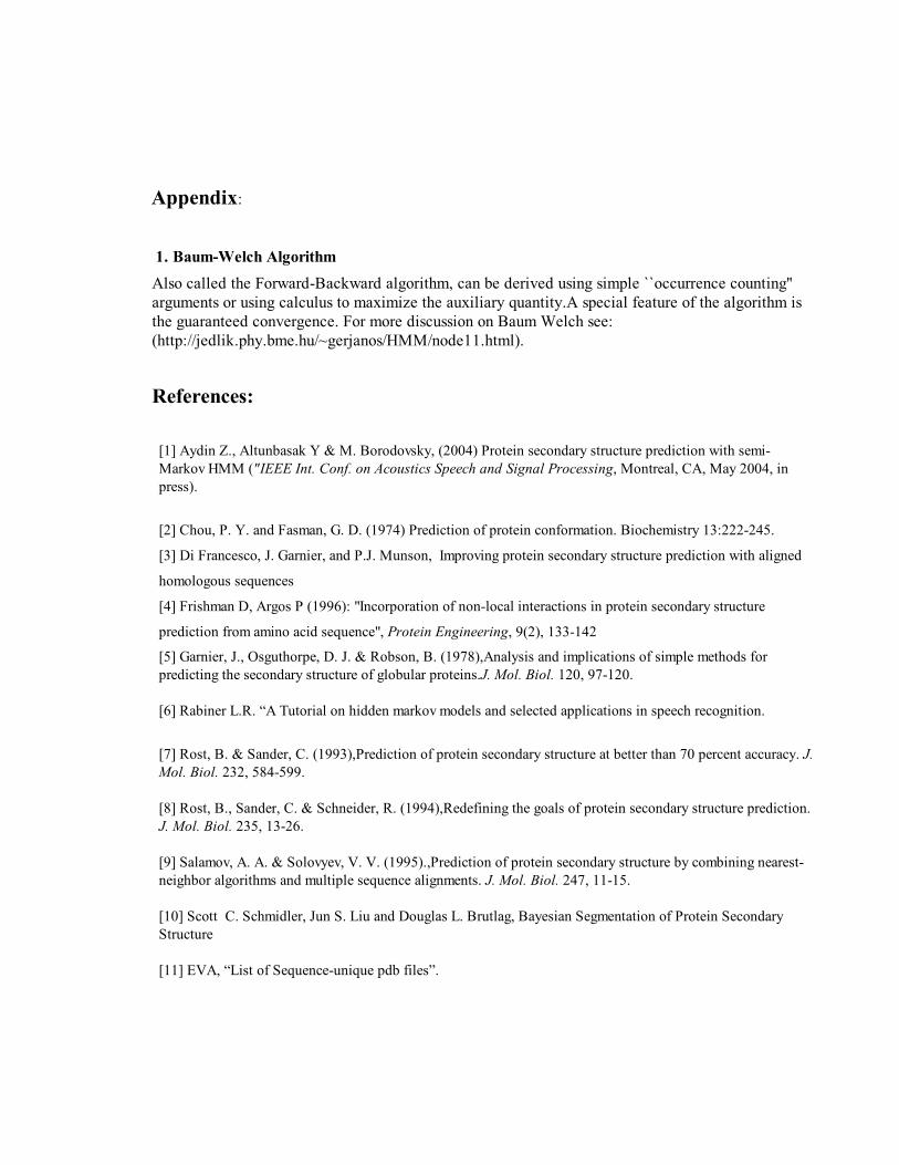
Appendix:

1. Baum-Welch Algorithm

Also called the Forward-Backward algorithm, can be derived using simple ``occurrence counting'' arguments or using calculus to maximize the auxiliary quantity.A special feature of the algorithm is the guaranteed convergence. For more discussion on Baum Welch see:(http://jedlik.phy.bme.hu/~gerjanos/HMM/node11.html).

References:

[1] Aydin Z., Altunbasak Y & M. Borodovsky, (2004) Protein secondary structure prediction with semi-Markov HMM ("IEEE Int. Conf. on Acoustics Speech and Signal Processing, Montreal, CA, May 2004, inpress).

[2] Chou, P. Y. and Fasman, G. D. (1974) Prediction of protein conformation. Biochemistry 13:222-245.

[3] Di Francesco, J. Garnier, and P.J. Munson, Improving protein secondary structure prediction with aligned

homologous sequences

[4] Frishman D, Argos P (1996): "Incorporation of non-local interactions in protein secondary structure

prediction from amino acid sequence", Protein Engineering, 9(2), 133-142

[5] Garnier, J., Osguthorpe, D. J. & Robson, B. (1978),Analysis and implications of simple methods forpredicting the secondary structure of globular proteins.J. Mol. Biol. 120, 97-120.

[6] Rabiner L.R. “A Tutorial on hidden markov models and selected applications in speech recognition.

[7] Rost, B. & Sander, C. (1993),Prediction of protein secondary structure at better than 70 percent accuracy. J.Mol. Biol. 232, 584-599.

[8] Rost, B., Sander, C. & Schneider, R. (1994),Redefining the goals of protein secondary structure prediction.J. Mol. Biol. 235, 13-26.

[9] Salamov, A. A. & Solovyev, V. V. (1995).,Prediction of protein secondary structure by combining nearest-neighbor algorithms and multiple sequence alignments. J. Mol. Biol. 247, 11-15.

[10] Scott C. Schmidler, Jun S. Liu and Douglas L. Brutlag, Bayesian Segmentation of Protein SecondaryStructure

[11] EVA, “List of Sequence-unique pdb files”.