lable at ScienceDirect

Atmospheric Environment 129 (2016) 34e42

Contents lists avai

Atmospheric Environment

journal homepage: www.elsevier .com/locate/atmosenv

Prospective air pollutant emissions inventory for the developmentand production of unconventional natural gas in the Karoo basin,South Africa

Katye E. Altieri*, Adrian StoneEnergy Research Centre, University of Cape Town, South Africa

h i g h l i g h t s

� Prospective emissions inventory for unconventional natural gas in South Africa.� Monte Carlo assessment of process-level and activity-level emissions estimates.� Shale gas development and production would dominate regional sources of NOx and NMVOC.

a r t i c l e i n f o

Article history:Received 20 October 2015Received in revised form8 January 2016Accepted 10 January 2016Available online 13 January 2016

Keywords:Shale gasNOx

PM2.5

NMVOCEmissions inventorySouth Africa

* Corresponding author. University of Cape Town,Cape Town, 7701, South. Africa.

E-mail address: katye.altieri@uct.ac.za (K.E. Altieri

http://dx.doi.org/10.1016/j.atmosenv.2016.01.0211352-2310/© 2016 Elsevier Ltd. All rights reserved.

a b s t r a c t

The increased use of horizontal drilling and hydraulic fracturing techniques to produce gas from un-conventional deposits has led to concerns about the impacts to local and regional air quality. South Africahas the 8th largest technically recoverable shale gas reserve in the world and is in the early stages ofexploration of this resource. This paper presents a prospective air pollutant emissions inventory for thedevelopment and production of unconventional natural gas in South Africa's Karoo basin. A bottom-upMonte Carlo assessment of nitrogen oxides (NOx ¼ NO þ NO2), particulate matter less than 2.5 mm indiameter (PM2.5), and non-methane volatile organic compound (NMVOC) emissions was conducted formajor categories of well development and production activities. NOx emissions are estimated to be 68tons per day (±42; standard deviation), total NMVOC emissions are 39 tons per day (±28), and PM2.5

emissions are 3.0 tons per day (±1.9). NOx and NMVOC emissions from shale gas development andproduction would dominate all other regional emission sources, and could be significant contributors toregional ozone and local air quality, especially considering the current lack of industrial activity in theregion. Emissions of PM2.5 will contribute to local air quality, and are of a similar magnitude as typicalvehicle and industrial emissions from a large South African city. This emissions inventory provides theinformation necessary for regulatory authorities to evaluate emissions reduction opportunities usingexisting technologies and to implement appropriate monitoring of shale gas-related activities.

© 2016 Elsevier Ltd. All rights reserved.

1. Introduction

Technological advancements over the past decade have led to arapid rise in unconventional natural gas production, known as“shale gas”, particularly in the United States and Canada. The large-scale and rapid development of shale gas production in these areashas resulted in an abundant and cheap energy source with lower

Private Bag X3, Rondebosch,

).

direct greenhouse gas (GHG) emissions than coal and petroleum,although the net GHG emissions impact is dependent upon thescale of methane leakage (Alvarez et al., 2012; Brandt et al., 2014).However, there have been concerns about the environmental im-pacts of unconventional natural gas development and productionon local water supplies (Vengosh et al., 2014), ambient air quality(Field et al., 2014; Moore et al., 2014), and human health (McKenzieet al., 2012). Such environmental concerns have led to bans on shalegas extraction in some countries and U.S. states (e.g., France andPennsylvania (Moore et al., 2014)), while other countries haveproposed various levels of regulations and recommendations (e.g.,the United Kingdom (U.K. Department of Energy and Climate

K.E. Altieri, A. Stone / Atmospheric Environment 129 (2016) 34e42 35

2013)). China is the only developing country that has pursued un-conventional natural gas exploration, and thus far has faced diffi-culties with respect to technology, water supply, and devisingappropriate regulatory structures (Hu and Xu, 2013).

South Africa has the 8th largest technically recoverable shale gasreserve in the world (U.S. Energy Information Administration,2013). It is located in three main formations in the Karoo basin,which covers 300 000 km2 of the interior of the country. This re-gion is underlain by a technically recoverable shale gas reserveestimated to be as large as 390 trillion cubic feet (TCF) (U.S. EIA,2013), with 20e50 TCF recoverable over a 25 year time period.The economic value of this deposit has been estimated to rangefrom 3.3 to 10.4% of GDP, while estimates of the number of new jobsthat could be created varies considerably from 1441 to 700 000(Econometrix, 2012;Wait and Rossouw, 2014). As an upper middle-income developing country with 28.9% unemployment (StatisticsSouth Africa, 2015a), the potential impacts on GDP and job crea-tion of the development of shale gas production are critical factorsto consider when evaluating environmental concerns.

Currently, natural gas contributes only 2.8% to primary energy inSouth Africa, and is primarily used to produce synthetic liquid fuels(Department of Energy (2009)). South Africa has large domesticcoal reserves, and coal contributes 65.9% to the primary energysupply (Department of Energy (2009)). As such, the development ofunconventional natural gas in South Africa could lead to a signifi-cant shift in the power and transport sectors by replacing coal-firedelectricity and providing liquefied natural gas (LNG) for heavy-dutyfreight and compressed natural gas (CNG) for light-duty vehicles(ERC Gas Report, 2015). In addition, bridging from coal to naturalgas could assist in South Africa's commitment to a peak, plateau,and decline GHG emissions trajectory (Department ofEnvironmental Affairs (2011)).

The Karoo basin in South Africa is a sparsely populated and vastarea, with low levels of industrial activity (Fig. 1). There is currentlyno air quality management plan and no ambient air quality moni-toring for this region. The exploration and development of un-conventional natural gas operations will likely have a dramaticimpact on the local population, environment, and economy(Kinnaman, 2011; Muehlenbachs et al., 2014; Steinzor et al., 2013;Vidic et al., 2013). Unconventional natural gas operations havethe potential for larger environmental impacts than conventionalgas operations due to the difficulty in extraction, as well as thediffuse nature of the resource. The lifespan of an unconventionalgas field includes exploration for 2e3 years, development for 3e5years, production for 10e30 years, and decommissioning for 5e10years (Government Accountability Office, 2012). Well densities arefrequently greater than one per km2, and the extent of the opera-tions can range from 100 000e300 000 km2. Each well site, whichincludes the drilling rigs, associated equipment, and pits to storedrilling fluids and waste, typically occupies an area of 10 000 m2.Due to the horizontal nature of the drilling, one well pad cansupport up to 50 drilled wells (IEA and World Energy Outlook,2012).

The time it takes to drill a well varies from 25 days in cases suchas the relatively shallow Barnett shale in Texas, where the work isbeing done by experienced operators (Armendariz, 2009), to 11months in cases such as China, where operations must contendwith difficult geology and inexperienced operators (Cohen, 2013).Unlike conventional wells, which have a steady decline rate of 5%per year, unconventional wells produce an initially large volume ofgas and then decline at a rate of 45e90% per year, essentiallyrunning dry after 1e3 years (IEA, 2011). As a result, new wells aredrilled regularly and once drilling commences in a shale play itcontinues 24 h a day, 7 days a week, 365 days a year. This creates aconstant output of noise, pollutants from diesel generators and

articulated engines, lights throughout the night, and 24-h trucktraffic. In addition, for the hydraulic fracturing (HF) process, eachwell requires 1000e50 000m3 of water that must be transported tothe site. Of this, 20e80% is returned via flow-back, at which point itis contaminated with the chemicals used in the HF process and alsocontains high levels of salts, metals, minerals, and hydrocarbons(Vengosh et al., 2014). The flow-back water requires treatment atindustrial wastewater treatment facilities and/or storage in on-siteponds or via injection into deep geological layers.

Unconventional natural gas exploration, production, anddevelopment results in a large number of relatively small sources ofair pollutants spread out over a potentially vast geographical area.The main pollutants from unconventional natural gas include ni-trogen oxides (NO þ NO2 ¼ NOx), non-methane volatile organiccompounds (hereafter, “NMVOCs”), and fine particulate matter(PM2.5; �2.5 mm in aerodynamic diameter). NOx and NMVOCs areprecursors to ozone, which could lead to significant regional effectson air quality as increased ozone is linked to asthma, decreasedlung function, and premature mortality (Levy et al., 2001).Increased PM2.5 leads to increased hospital admissions, respiratorysymptoms, chronic respiratory and cardiovascular diseases,decreased lung function, and premature mortality ((Kim et al.,2015) and references therein). The aggregate emissions from themultitude of small sources can thus be significant for local healthand regional ambient air quality, especially with respect to ozoneproduction. For example, the Dallas-Fort Worth area within theBarnett shale zone has seen increases in short-term and long-termozone trends in shale gas areas, as compared to areas without shalegas wells (Ahmadi and John, 2015). In addition, there have evenbeen episodes of winter ozone related to shale gas activities inWyoming and Utah, which is highly unusual, with values thatexceeded US National Ambient Air Quality Standards (Field et al.,2015; Schnell et al., 2009).

Emissions inventories can be used for establishing regulations,devising enforcement strategies and health risk assessments, as apredictive tool to establish monitoring strategies, and as inputs toregional air quality models. An emissions inventory can also assistin evaluating environmental impacts, but it cannot substitute forthe critical information gained from ambient monitoring and per-sonal exposure monitoring once activities have commenced. Thework presented here aims to develop a prospective air pollutantemissions inventory for NOx, PM2.5, and NMVOCs associated withunconventional natural gas production and development in theKaroo basin.

2. Materials and methods

This study was conducted using an in-silico bottom-up approachto create an emissions inventory for unconventional natural gasdevelopment and production in the Karoo basin, following theapproach of (Roy et al., 2014) and references therein. Methane wasexcluded from the NMVOC inventory as the focus was not on GHGemissions. Process-level emissions are time independent and applywhenever the unconventional natural gas exploration and devel-opment commences. Basin-scale emissions depend on the rate ofdevelopment of wells over time and the scale of the resourceexploitation.

The unconventional natural gas industry in South Africa is still atthe exploration stage, and well development and production havenot yet commenced. In this study, emissions were estimated for thetwo main categories of well development and well production.Well development includes drilling the well, hydraulically frac-turing the well, all of the trucking activities related to transportingequipment and water to and from the well, and the completionventing process. Drilling the well includes the construction of the

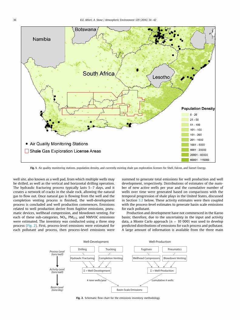
Fig. 1. Air quality monitoring stations, population density, and currently existing shale gas exploration licenses for Shell, Falcon, and Sunset Energy.

K.E. Altieri, A. Stone / Atmospheric Environment 129 (2016) 34e4236

well site, also known as a well pad, fromwhich multiple wells maybe drilled, as well as the vertical and horizontal drilling operation.The hydraulic fracturing process typically lasts 5e7 days, and itcreates a network of cracks in the shale rock, allowing the naturalgas to flow out. Once natural gas is flowing from the well and thecompletion venting process is finished, the well-developmentprocess is concluded and well production commences. Emissionsrelated to well production derive from fugitive emissions, pneu-matic devices, wellhead compression, and blowdown venting. Foreach of these sub-categories, NOx, PM2.5, and NMVOC emissionswere estimated. The inventory was conducted using a three stepprocess (Fig. 2). First, process-level emissions were estimated foreach pollutant and process, then process-level emissions were

Fig. 2. Schematic flow chart for the e

summed to generate total emissions for well production and welldevelopment, respectively. Distributions of estimates of the num-ber of new active wells per year and the cumulative number ofwells over time were generated based on comparisons with thetemporal progression of shale plays in the United States, discussedin Section 3.2 below. These activity estimates were then coupledwith the process-level estimates to generate basin scale emissionsfor each pollutant.

Production and development have not commenced in the Karoobasin; therefore, due to the uncertainty in the input and activitydata, a Monte Carlo approach (n ¼ 10 000) was used to developpredicted distributions of emissions for each process and pollutant.A large amount of information is available from the three main

missions inventory methodology.

K.E. Altieri, A. Stone / Atmospheric Environment 129 (2016) 34e42 37

shale plays in the United States, i.e., the Haynesville, Barnett, andMarcellus shales, and there are similarities between the depth andthickness of the South African shale plays and the already-exploitedplays in the United States. For example, the depth of the three SouthAfrican shale formations, which range from 2.4 to 2.6 km(7800e8500 feet), are on average slightly deeper than the Barnettshale (1.98e2.6 km; 6500e8500 feet), but shallower than theHaynesville shale (3.2e4.1 km; 10 500e13 500 feet). The thicknessranges from 24 to 37 m (80e120 feet), which is similar to theMarcellus and Barnett shales. These similarities provide a range ofinputs for the length of time and number of stages required to drilland hydraulically fracture a well in South Africa. The sources,values, and distributions of all input parameters (Table 1 andTables Se1) are discussed in more detail below for each processassociated with well development and production.

3. Results and discussion

3.1. Process-level emissions

The emissions associated with each step of developing a welland bringing the well into production are the process-level emis-sions. Emissions from condensate tanks are excluded as South Af-rican shale gas is assumed to be a predominantly dry gas resource(U.S. Energy Information Administration, 2013).

3.1.1. Well development emissions3.1.1.1. Drilling. The drilling of a well requires multiple engines,typically 5 to 7 diesel-fired compression-ignition engines per well.These engines are usually 300e1000 kW (kW) (500e1500 horse-power (hp)), and include draw-works engines, mud pump engines,and generator engines. The draw-works engine provides power tothe rotating drill bit that performs the cutting operations. Themud-pump engine pumps mud into the borehole for lubrication andcooling. The generator engine provides power to the drilling crewand supports all the power needs of the entire well-site operation.The process-level drilling emissions were calculated using Eq. (1)

Table 1Values and distributions of input parameters used in drilling, fracking, trucking, and comminimum, parameter 2 is the most likely value, and parameter 3 is the maximum. Forstandard deviation. For uniform distributions, the minimum and maximum are providedistribution, parameter 1 is the location parameter and parameter 2 is the shape param

Pollutant Variable Distribution

DrillingNOx EF (g kWh�1) TriangularPM2.5 EF (g kWh�1) TriangularNMVOCs EF (g kWh�1) Triangular

Total Kilowatts (kW) NormalLoad Factor TriangularDrilling time (days) Extreme ValuePercent on-time Triangular

Hydraulic FracturingNOx EF (g kWh�1) TriangularPM2.5 EF (g kWh�1) TriangularNMVOCs EF (g kWh�1) Triangular

Total Kilowatts (kW) TriangularLoad Factor Point Value# Stages per well Triangular

TruckingNOx EF (g km�1) UniformPM2.5 EF (g km�1) TriangularNMVOCs EF (g km�1) Triangular

Trips per well TriangularDistance to well and waste (km) Triangular

Completion VentingNMVOCs MCF completion event�1 Triangular

Mass fraction dry gas Uniform

(Grant et al., 2009; Roy et al., 2014):

Edrilling ¼ EFi � kW � LF � tdrilling � %on�time (1)

where the emissions factor (EF) is for a given pollutant (i), the en-gine size in kW is the combined kW for all engines used to drill thewell, the load factor (LF) is the average engine output as a per-centage of the rated engine power, and the % on-time (%on-time) isthe percentage of the drilling time (tdrilling; defined below) duringwhich the drilling operation is active.

The values and distributions used (Table 1) are based in part onthe range of values reported for well drilling in the Marcellus,Barnett, and Haynesville shales (Armendariz, 2009; Grant et al.,2009; Roy et al., 2014). The goal in determining the distributionsof engine properties and emissions factors was to include the entirerange of possibilities for the Karoo basin. For example, the range inemissions factors includes values from the United States Environ-mental Protection Agency AP-42 database, the East Texas Basin drillrig configuration, engine surveys conducted by the Texas Com-mission on Environmental Quality on local unconventional naturalgas operations, as well as controlled and uncontrolled emissionsfrom the Australian Department of the Environment (Armendariz,2009; Grant et al., 2009; Roy et al., 2014). This reflects the fullrange of possible emissions factors for drilling engines that mightbe deployed in the Karoo basin, with the higher values representinga lack of control regulations and the lower values representing amore stringent regulatory environment. The engine size, load fac-tor, and % on-time values were taken from the range of values foractual drilling operations in the Marcellus, Barnett, and Haynesvilleshales (Table 1), and these parameters can be considered specific tounconventional natural gas drilling, and not specific to a particularbasin's characteristics.

The time to drill one well in the Karoo basin (tdrilling) wascalculated based on the relationship between the depth of theshales in the three main plays in the United States and the numberof days required to drill one well (Armendariz, 2009; Grant et al.,2009; Roy et al., 2014), as well as information from China on

pletion venting emissions estimates. For triangular distributions, parameter 1 is thenormal distributions, parameter 1 is the numerical average and parameter 2 is thed as parameter 1 and parameter 2, respectively. For the extreme continuous valueeter.

Parameter 1 Parameter 2 Parameter 3

2.68 7.78 21.460.09 0.47 1.340.34 0.80 2.153254 6790.25 0.57 0.932.9 10.10.2 0.25 1

3.35 7.64 13.410.12 0.54 1.210.40 0.90 2.15373 746 26100.54 19 35

1.48 11.470.02 0.09 0.230.02 0.20 0.57495 1121 23400 350 800

18 3700 24 0000.005 0.059

K.E. Altieri, A. Stone / Atmospheric Environment 129 (2016) 34e4238

drilling times and depths (Hu and Xu, 2013). The depths of the USand Chinese shales were plotted as a linear function of averagedrilling time (y ¼ 0.005x-3.6; r2 ¼ 0.9634). This equation was thenapplied to the range of depths for the threemain Karoo basin shales(U.S. Energy Information Administration, 2013) in order to calculatea range in the number of days to drill one well in the Karoo basin.The resulting values were fit with a probability distribution usingmaximum likelihood estimators (@RISK Palisade Corporation). Forthe drilling days, the extreme value fit was the highest ranked fitusing the Akaike information criteria (Table 1; SupplementalFigs. Se1), and this fit was confirmed by examining the linearityof the probabilityeprobability graph as well as the quanti-leequantile graph. Furthermore, the extreme value fit seems themost appropriate distribution as it includes the possibility oflengthy drilling times, which occurred in China with inexperiencedoperators and difficult geology (Cohen, 2013). Unlike in the UnitedStates, there currently exists no conventional oil or gas industry inSouth Africa, such that the assumption of inexperienced operatorsis valid in this case.

The mean and 95% confidence interval from process-level dril-ling emissions for NOx PM2.5, and NMVOCs are presented (Table 2).The mean is presented for reference; however, the confidence in-terval represents the variability inherent in the input parameters(Table 1) and is the most appropriate quantification of the range ofpossible emissions given the uncertainty in inputs. The average NOx

emissions are 9.8 tons/well, with a 95% confidence interval of2.3e24.1 tons/well (presented as mean (95% confidence interval)throughout), the average PM2.5 emissions are 0.59 tons/well(0.12e1.5), and the average NMVOC emission are 1.01 tons/well(0.25e2.5). The drilling emissions estimated in this work are higherthan those for shale plays in the United States. For example, in theMarcellus shale, drilling-related NOx emissions are estimated toaverage 4.4 tons/well, with a 95% confidence interval of 0.8e11.5tons/well (Roy et al., 2014). The differences are due to the slightlyhigher emissions factors used in this work, as well as the longerdrilling times required by the greater depths of the Karooformations.

3.1.1.2. Hydraulic fracturing. Hydraulic fracturing (HF) occurs afterthe drilling of the well bore to stimulate the production of naturalgas. Pump engines are used to push large quantities of fracking fluid(a typically-proprietary mixture of water, sand, and chemicals) intothe well bore to hydraulically fracture the rock formation, releasingthe natural gas. The HF process-level emissions were calculatedusing Eq. (2):

EHF ¼ EFi � kW � LF � Nstages (2)

where the emissions factor (EF) is for a given pollutant (i) for onepump engine, the engine size in kW is the combined kW to hy-draulically fracture one stage, the load factor (LF) is the average loadfactor for one pump engine, and the number of stages (Nstages) is thetotal number of stages needed to hydraulically fracture one well,which depends on the length of the horizontal component of the

Table 2Average (95% confidence interval) process-level emissions of NOx, PM2.5, andNMVOCs from the development of unconventional natural gas wells in the Karoobasin.

Emissions (tons/well) NOx PM2.5 NMVOC

Drilling 9.8 (2.3e24.1) 0.59 (0.12e1.5) 1.01 (0.25e2.5)Hydraulic Fracturing 2.6 (0.77e5.6) 0.20 (0.05e0.45) 0.37 (0.10e0.83)Trucking 7.2 (1.6e16.7) 0.13 (0.03e0.28) 0.29 (0.06e0.67)Completion Venting n/a n/a 6.1 (0.81e16.3)

well. The range of values used was based upon wells that haveundergone the HF process in the Marcellus, Barnett, and Haynes-ville shales (Armendariz, 2009; Grant et al., 2009; Roy et al., 2014).Process-level HF emissions are significantly lower than drillingemissions for all pollutants (Table 2). Values calculated for theKaroo basin are similar in magnitude to those for the Marcellusshale (Roy et al., 2014), although as with drilling emissions, thevalues here are slightly higher.

3.1.1.3. Trucking. Truck traffic will increase substantially with theexploration and development of unconventional natural gas. Trucksare used initially to transport all of the necessary materials to thewell site, including the engines, water, chemicals, and equipment.In the USA, tractor-trailers (i.e., large articulated trucks) are usedalmost exclusively for moving this type of equipment. In addition,trucks are used to transport materials from one well to another asneeded. A potentially large source of truck traffic, and one with aconsiderable amount of uncertainty in South Africa, is associatedwith the transport of water to the well for HF, as well as the transferof flow-back water to wastewater treatment sites or storage ponds.

Process-level trucking emissions were calculated using Eq. (3):

Etrucking ¼ EFi � D� Ntrips (3)

where the emissions factor (EF) is for a given pollutant (i), the totaldistance travelled (D) includes round trip distances, and the num-ber of trips (Ntrips) includes all trips needed to bring the well up toproduction and to transport water to and from the well site. Theemissions factors for trucking were calculated using COPERT IVHDV articulated truck equations for a 0% gradient, 0e50% loadfactor, and assuming an average speed of 60 km h�1. The tonnage ofthe trucks was allowed to range from a gross weight of 28e40 tons,and the standards ranged from Euro-2, South Africa's minimumemissions standard, to Euro-4, which the National Association ofAutomobile Manufacturers of South Africa (NAAMSA) sales datashow is the range of standards being imported for this weightrange, with Euro-3 the most common (data from Lightstone Auto,2015). The resultant calculated emissions factors for NOx rangefrom 2.11 g km�1 to 10.85 g km�1, with a uniform fit determinedusing maximum likelihood estimators (Table 1). Calculated emis-sions factors for PM2.5 and NMVOCs range from 0.02 to 0.19 g km�1

and 0.016e0.428 g km�1, respectively, with triangular distributionsproviding the best fit (Table 1).

The number of trips per well is difficult to estimate as it dependson a variety of factors that are yet to be determined including thelocation of the wells, where equipment is sourced from and stored,the distance between wells, the source of water, etc. Roy et al.(2014) utilized truck trip data from the US National Park Service,and estimated that drill pad and road construction equipment took10 to 45 trips, the drilling rig set up took ~ 30 trips, the drilling fluidandmaterials transport required 25 to 50 trips, other miscellaneoustrips ranged from 30 to 40, and the fracture stimulation fluid,materials, and equipment transport required 200 to 1150 trips. Thehauling of wastewater could take an additional 200 to 1000 trips,depending on the amount of flow-back, which varies across wells,and the method of treating or storing the wastewater. For example,if wastewater is stored on site in storage ponds, there may be verylittle truck traffic after the initial well development. To account forthis uncertainty, a large range of the number of trips per well wasallowed (Table 1), and this led to considerable uncertainty in therange of trucking emissions. Similarly, the distances travelled pertrip were difficult to estimate without information on locations andstrategies for handling equipment and water (Table 1). The goal ofthis work is not to correctly estimate trucking distances, but toinstead provide emission estimates across the range of possible

K.E. Altieri, A. Stone / Atmospheric Environment 129 (2016) 34e42 39

distances travelled and number of trips to develop the well andtransport water and wastewater.

As a result of these uncertainties in input data, and to provide atheoretically possible range in emissions, the trucking emissionsare presented as a function of distance travelled (Fig. 3). The 95%confidence interval of trucking emissions for NOx, PM2.5, andNMVOCs all range across roughly one order of magnitude as dis-tance increases from 0 to 600 km (Fig. 3). Once distances are knownwith more certainty, Fig. 3 can be used to determine a likely rangeof trucking emissions. Allowing the trucking emissions to rangeacross their probable values (Table 1), the average trucking NOxemissions are 7.2 (1.6e16.7) tons/well (Table 2), which is similar inmagnitude to drilling emissions estimated for the Karoo basin(section 3.1.1.1), and also similar to trucking emission in the Mar-cellus basin (Roy et al., 2014). The average PM2.5 trucking emissionsare 0.13 (0.03e0.28) tons/well (Table 2), which are lower thandrilling and HF emissions, but similar to Marcellus emissions (Royet al., 2014). The average NMVOC trucking emissions are 0.29(0.06e0.67) tons/well (Table 2), which are also lower than drillingand HF emissions, and lower than Marcellus emissions (Roy et al.,2014). The differences from the Marcellus emissions derive from

0

5

10

15

20

25

0 100 200 300 400 500 600

NO

Emiss

ions

(ton

s/well)

Distance Traveled (km)

Mean

5%

95%

a)

0.00

0.05

0.10

0.15

0.20

0.25

0.30

0.35

0.40

0.45

0 100 200 300 400 500 600

PMEm

issions

(ton

s/well)

Distance Traveled (km)

Mean

5%

95%

b)

0.00

0.10

0.20

0.30

0.40

0.50

0.60

0.70

0.80

0.90

1.00

0 100 200 300 400 500 600

NMVO

CEm

issions

(ton

s/well)

Distance Traveled (km)

Mean

5%

95%

c)

Fig. 3. Trucking-related a) NOx, b) PM2.5, and c) NMVOC emissions for well develop-ment, including the transport of water to and from the wells, as a function of distancetravelled. Note the different y-axis scales for each pollutant.

the differences in the estimated distances travelled, and the SouthAfrica-specific emissions factors.

3.1.1.4. Well completions. The well completion process is necessaryto produce gas from the well, and it occurs after the drilling and HFactivities have been completed. It requires venting the well for asustained period of time to remove any debris or mud and toremove any inert gases present from the well stimulation process.The well completion process brings the gas composition to pipelinegrade for transport and consumer use. This process can result in asignificant amount of vented gas, and as such can be a large sourceof NMVOCs. Green completions and flaring are two techniques thatcan reduce emissions by up to 95% during the well completionprocess. For this analysis, it is assumed that no control measureswere utilized initially, partially due to the Karoo basin having aprimarily dry gas resource (U.S. Energy Information Administration,2013). Well completions will lead to much lower levels of NMVOCsthan if wet-gas were present due to the differences in NMVOCcontent. Emissions of NMVOCs from well completions werecalculated using Eq. (4):

Ecompletion venting ¼

P � V�R=MW

�� T

!� fi (4)

where P is the atmospheric pressure, R is the universal gas constant,MW is the molecular weight of the gas, T is the atmospheric tem-perature, V is the volume of gas vented per completion event, and fiis the mass fraction of NMVOCs in the vented gas (Table 1). Themass fraction of NMVOCs for dry-gas is typically 0.5e5% (Roy et al.,2014), although this value will have to be updated once measure-ments are taken of natural gas extracted from the Karoo basin. Thevolume of gas vented per completion event varies dramatically,from estimates of 2417 MCF event�1 in the Haynesville shale (Grantet al., 2009), to 5000MCF event�1 in the Barnett shale (Armendariz,2009), and an average of 3700 MCF event�1 in the Marcellus shalewith a range of 18e24 000 (Roy et al., 2014).

The average completion venting emissions of NMVOCs are 6.1tons/well (0.81e16.3; Table 2). This is by far the largest source ofNMVOCs fromwell development. The 5% confidence interval valueof 0.81 tons/well is similar to the 95% confidence interval values ofthe other development activities. However, if the Karoo basin had awet-gas resource, this value would be much higher. The Marcellusshale, which has a mixture of dry- and wet-gas areas, hascompletion venting emissions as high as 145 tons/well due to thepresence of wet gas (Roy et al., 2014).

3.1.2. Well production emissionsProduction emissions are primarily NMVOC emissions, except in

the case of the use of wellhead compressors, which also releasesmall amounts of NOx and PM2.5. NMVOCs are released from pro-duction fugitives, pneumatic devices, and blowdown venting.Production emissions are assumed to derive from devices andcompressors that operate all year (i.e., 8760 h). Input parametersare not typically specific to a well (Tables Se1), although theyshould be measured when wells become operational. The valuesused here were taken from (Roy et al., 2014), which largely usedvalues from (Grant et al., 2009) and references therein. Wellheadcompressor NOx and PM2.5 emissions are fairly small compared towell development emissions (Table 3). Production NMVOC emis-sions are also fairly small (Table 3). Indeed, if all NMVOC emissionsfrom production are summed with their uncertainties, the averageis 0.78 (0.3e1.26) tons/well, which is comparable toMarcellus shaleemissions, as would be expected from the similarities in the input

Table 3Average (95% confidence interval) process-level emissions of NOx, PM2.5, and NMVOCs from the production of unconventional natural gas.

Emissions (tons/well) NOx PM2.5 NMVOC

Production fugitives n/a n/a 0.089 (0.021e0.18)Pneumatic devices n/a n/a 0.63 (0.15e1.1)Wellhead compressors 1.5 (0.74e2.4) 0.015 (0.004e0.03) 0.020 (0.006e0.04)Blowdown venting n/a n/a 0.04 (0.005e0.11)

0

0.1

0.2

0.3

0.4

0.5

0.6

0.7

0.8

0.9

1

0 10 20 30 40 50 60 70 80 90 100NOxDevelopment and Produc on Emissions (tons/well)

Mean

5%

95%

a)

0

0.1

0.2

0.3

0.4

0.5

0.6

0.7

0.8

0.9

1

0 0.5 1 1.5 2 2.5 3 3.5 4 4.5 5 5.5 6PM2.5 Development and Produc on Emissions (tons/well)

Mean

5%

95%

b)

0

0.1

0.2

0.3

0.4

0.5

0.6

0.7

0.8

0.9

1

0 5 10 15 20 25 30 35NMVOC Development and Produc on Emissions (tons/well)

Mean

5%

95%

c)

Fig. 4. Cumulative distribution functions of total development and production emis-sions of a) NOx, b) PM2.5, and c) NMVOCs in tons per well. The mean and 95% confi-dence intervals are presented. Note the different x-axis scales.

K.E. Altieri, A. Stone / Atmospheric Environment 129 (2016) 34e4240

data (Roy et al., 2014).

3.2. Karoo basin-scale emissions

The drilling, trucking, hydraulic fracturing, and completionventing emissions for each pollutant were summed to determinetotal well-development emissions. Total well-development NOxemissions average 19.6 tons/well (8.5e36.0), PM2.5 emissionsaverage 0.91 tons/well (0.38e1.8), and NMVOC emissions average7.8 tons/well (2.2e18.3). Well-development emissions are higherfor all pollutants than well-production emissions. Total well-production NOx emissions average 1.47 (0.73e2.38), PM2.5 emis-sions average 0.015 (0.004e0.03), and NMVOC emissions average0.78 (0.29e1.26). Overall, the distribution of input parameters leadsto wide ranges in total NOx, PM2.5, and NMVOC emissions for thedevelopment and production of one well in the Karoo basin (Fig. 4).

Scaling up the well-development emissions to generate esti-mates of basin-wide emissions required estimating the totalnumber of wells that may be developed. The first step in explora-tion and production is to establish drill rigs. The number of drill rigsincreases over time as a function of many variables including, butnot limited to, domestic economic factors, natural gas prices,equipment availability, and success rates. In other shale plays, thegrowth rate of drill rigs has ranged from 0 to ~25 per year, althoughthe variability is large (Grant et al., 2009). The area of the Karoobasin that may be explored is 155 000 km2, which is much largerthan the Barnett and Haynesville shale plays (13 000 and23 000 km2, respectively), but smaller than the Marcellus shale(250 000 km2). The success rate for each drill rig is typically only55% in the early years, although it is assumed to increase to almost100% after 10 years of exploration. Assuming a rig growth rate witha triangular distribution of 0e25 rigs per year with 12 rigs per yearsas the most likely value, success rates that increase linearly from 55to 100% over ten years, and using the distribution of days to drillone well in South Africa (Table 1), results in an estimated range of565e2848, with an average of 1412 new active unconventionalnatural gas wells per year in South Africa in year ten of explorationand development. These numbers are highly uncertain, althoughsimilar in magnitude to other regions. For example, the Haynesvilleshale area had 1200 new active wells after ten years (Grant et al.,2009), while the Marcellus shale had 5000 new active wells afterfar fewer than ten years (Roy et al., 2014). The number of new activewells each year was used to scale up well development-relatedactivities, and was then summed to calculate the cumulativenumber of wells active in year ten, whichwas the scaling parameterused for well production activities.

The number of new and cumulative wells were then combinedwith the process-level emissions estimates to calculate basin-scaleNOx, PM2.5, and NMVOC emissions estimates in tons per day (Fig. 5,Figure S-2). NOx is the largest contributor to development andproduction emissions, with an average of 68 tons/day (±42; stan-dard deviation). Basin-scale NOx emissions are dominated by welldevelopment activities, particularly drilling and trucking. NMVOCemissions average 39 tons/day (±28), with completion venting andpneumatic devices generating the largest emissions. PM2.5 emis-sions are significantly lower than NMVOCs and NOx, with an

average of 3.0 tons/day (±1.9). Drilling is by far the largest source ofPM2.5 emissions, accounting for 62% of basin-scale PM2.5 emissions(Supplemental Figs. Se2).

The NOx emissions are similar in magnitude to current dayemissions from the Haynesville shale, 57e63 tons/day (Grant et al.,2009), and the Barnett shale, 56 tons/day (Armendariz, 2009). Inthe Haynesville area, shale gas emissions are the dominant sourceof NOx. In the Barnett shale area, NOx and NMVOC emissions from

0

20

40

60

80

100

120

COVMN5.2MPxON

Emissions

(tons/day)

Blowdown Ven ng

Pneuma c Devices

Produc on Fugi ves

Comple on Ven ng

Wellhead Compressors

Trucks

Fracking

Drilling

Fig. 5. Average development and production emissions of NOx, PM2.5, and NMVOCs intons per day for all major activity categories (colours in legend) with the standarddeviation of the total summed emissions denoted by the black vertical lines.

K.E. Altieri, A. Stone / Atmospheric Environment 129 (2016) 34e42 41

shale gas activities are significantly higher than those associatedwith the large airport located nearby, and larger than on-roadmobile sources. Even in areas with high population density andother active industries, unconventional natural gas-related emis-sions are a significant contributor to the regional NOx and NMVOCemissions budgets.

3.2.1. Comparison to regional and national emission inventoriesThe Karoo basin spans the Western, Eastern, and Northern Cape

provinces of South Africa. Provincial level emissions inventories arenot published regularly, rendering comparisons to the shale gasemissions inventory difficult. Indeed, the lack of comprehensiveemissions inventories is stated as the greatest inhibitor of airquality management in these regions. The Northern Cape occupies33% of South Africa, although its population is sparse at 1 millionpeople (Statistics South Africa, 2015b). Emissions are likely limitedto transport corridors, soil NOx, and some mining activities thatmay contribute to coarse PM emissions (i.e., >2.5 mm in aero-dynamic diameter). The Eastern Cape has a population of 6.5million and occupies 13.9% of South Africa (Statistics South Africa,2015b). Industrial and manufacturing activities in proximity to itsthree main ports are likely to be the main emissions sources, andthe province accounts for 7.8% of national vehicular emissions.However, no detailed emissions inventories are available for theEastern or Northern Cape provinces.

The Western Cape has 5.8 million people and occupies 10% ofthe area of South Africa (Statistics South Africa, 2015b). In 2011, theWestern Cape government published an emissions inventory con-structed from a total of 1249 industries with fuel burning appli-ances, as well as 597 gasoline/petrol filling stations. There are only4 point sources and 11 filling stations within the Central Karoodistrict municipality, the area closest to where the shale gasexploration and development will take place. The vast majority ofindustries and filling stations in the Western Cape are within theCity of Cape Town, population 3.7 million, which is ~500 km fromthe Karoo. The total Western Cape emissions of NOx are 13.12 tons/day. From the Central Karoo district municipality, NOx emissionsare estimated to be only 0.002 tons/day. Even at its lowest estimate,NOx emissions from unconventional natural gas development andproduction will dominate regional emissions, including in the Cityof Cape Town, which hosts a port, airport, and high vehicle trafficburden. Western Cape NMVOC emissions total 0.295 tons/day,which are also significantly lower than the estimates presentedhere for the production and development of shale gas.

An additional comparison can be done with the city of Durban,

which has a population of 3.4 million people. The shale gasdevelopment and production NOx emissions, average of 68 tons/day (18e147; 5%e95% CI), are comparable to the largest source inthe city of Durban, which is aircraft at 89 tons/day, and significantlyhigher than the estimates of diesel and petrol vehicles and indus-trial activity at 37, 25, and 20 tons/day (FRiDGE, 2004). Emissions ofPM2.5 from shale gas activities, average of 3.0 tons/day (0.77e6.5),are small compared to Durban city-wide emissions, which aredominated by aircraft at 19 tons/day, and diesel vehicles and in-dustrial activity at 10 and 7 tons/day, respectively.

Nationally, the largest source of NOx emissions in South Africa iscoal-fired electricity generation. Over 95% of South Africa's elec-tricity is generated by one parastatal utility company, Eskom, andthe year-end reports provide information on the amount of NOxemitted per year from the power sector. Eskom estimates that 4.22tons of NOx are emitted per GWh of power generated (1172 tons/PJ),which, given the 228 208 GWh of power generated nationally peryear, amounts to 2638 tons of NOx per day from power generation.This value is consistent with a national emissions inventory from2006, where electricity generation was the largest source of NOx at1883 tons/day, followed by industrial and commercial fuel burningat 789 tons/day, vehicles at 730 tons/day, and shipping, aircraft,biomass and domestic fuel burning all at less than 10 tons/day(Scorgie and Venter, 2006). The NOx emissions from shale gasdevelopment and production estimated here, with an average of 68tons/day and 95% confidence interval of 18e147 tons/day, would bethe 4th largest NOx source in the country as compared to the 2006inventory. The largest source of NMVOC emissions in the nationalinventory is vehicles at 318 tons/day, followed by biomass burningat 9 tons/day and electricity generation at 7 tons/day (Scorgie andVenter, 2006). Shale gas development and production, with anaverage of 38 tons/day and a 95% confidence interval of 9.3e91tons/day, would be the second largest national source of NMVOCs.PM2.5 emissions from shale gas development and production arequite small compared to the national inventory values and wouldnot be a significant contributor. However, given that there iscurrently no significant source of PM2.5 in the Karoo basin, thepotential detrimental effect(s) of an increase in this pollutant onhuman health in the region should not be ignored.

4. Conclusions

There is currently very little industrial activity in the Karoo basinin South Africa. The exploration, development, and production ofthe potentially large shale gas resource in this area, 20 to 50 TCFover 25 years, will likely lead to dramatic changes in the region,including significant increases in air pollutant emissions. Here, wepresent ranges of NOx, PM2.5, and NMVOC emissions calculatedfrom Monte Carlo simulations of all possible input parameters. Wefind that the shale gas industry will likely become the largestregional source of NOx and NMVOCs, although a minor source ofPM2.5. Even if the lowest estimate of NOx emissions is used, i.e., the5% confidence level, shale gas development and production wouldbe the 4th largest source of NOx nationally. Similarly, NMVOCs fromshale gas activities would be the second largest source of NMVOCsin the country. The relative contribution and range of values frommajor development and production process-level emissions of NOx,PM2.5, and NMVOC emissions provides information on how regu-lations can be used to reduce emissions. The high estimated valuesof NOx and NMVOC emissions are a concern for regional impacts onozone formation and ambient air quality compliance. Local emis-sions of PM2.5, as well as NOx and NMVOCs, will contribute nega-tively to local air quality and could have human health impacts. Thisemissions inventory will be a critical input to air quality modelling,which will be required to evaluate the local and regional impacts of

K.E. Altieri, A. Stone / Atmospheric Environment 129 (2016) 34e4242

unconventional natural gas activities on ambient air quality. Newmonitoring stations will be needed closer to the industrial activitiesonce they commence to provide ambient data and to allow formodel verification. There are a variety of control technologiesavailable to limit NOx and NMVOC emissions, and these should beinvestigated fully to reduce the impact of shale gas activities onlocal, regional, and national air quality in South Africa.

Acknowledgements

The Energy Research Centre acknowledges the Neale Trust forfunding.

Appendix A. Supplementary data

Supplementary data related to this article can be found at http://dx.doi.org/10.1016/j.atmosenv.2016.01.021.

References

Ahmadi, M., John, K., 2015. Statistical evaluation of the impact of shale gas activitieson ozone pollution in north Texas. Sci. Total Environ. 536, 457e467. http://dx.doi.org/10.1016/j.scitotenv.2015.06.114.

Alvarez, R.A., Pacala, S.W., Winebrake, J.J., Chameides, W.L., Hamburg, S.P., 2012.Greater focus needed on methane leakage from natural gas infrastructure. Proc.Natl. Acad. Sci. U. S. A. 109, 6435e6440. http://dx.doi.org/10.1073/pnas.1202407109.

Armendariz, A., 2009. Emissions from Natural Gas Production in the Barnett ShaleArea and Opportunities for Cost-Effective Improvements (Austin, TX).

Brandt, A.R., Heath, G.A., Kort, E.A., O'Sullivan, F., P�etron, G., Jordaan, S.M., Tans, P.,Wilcox, J., Gopstein, A.M., Arent, D., Wofsy, S., Brown, N.J., Bradley, R.,Stucky, G.D., Eardley, D., Harriss, R., 2014. Energy and environment. Methaneleaks from north American natural gas systems. Science 343, 733e735. http://dx.doi.org/10.1126/science.1247045.

Cohen, A.K., 2013. The Shale Gas Paradox: Assessing the Impacts of the Shale GasRevolution on Electricity Markets and Climate Change (No. 14). Mossavar-Rahmani Center for Business and Government.

R. of S.A Department of Energy, 2009. Digest of South African Energy Statistics(South Africa).

Department of Environmental Affairs, 2011. The Government of the Republic ofSouth Africa National Climate Change Response White Paper.

Econometrix, 2012. Special Report on Economic Considerations Surrounding Po-tential Shale Gas Resources in the Southern Karoo of South Africa.

Field, R.A., Soltis, J., McCarthy, M.C., Murphy, S., Montague, D.C., 2015. Influence ofoil and gas field operations on spatial and temporal distributions of atmo-spheric non-methane hydrocarbons and their effect on ozone formation inwinter. Atmos. Chem. Phys. 15, 3527e3542. http://dx.doi.org/10.5194/acp-15-3527-2015.

Field, R.A., Soltis, J., Murphy, S., 2014. Air quality concerns of unconventional oil andnatural gas production. Environ. Sci. Process. Impacts 16, 954e969. http://dx.doi.org/10.1039/c4em00081a.

FRiDGE, 2004. Bentley West Management Consultants (Pty) Ltd and Airshed Plan-ning Professionals (Pty) Ltd: Study to Examine the Potential Socio-economic

Impact of Measures to Reduce Air Pollution from Combustion.Government Accountability Office, 2012. Gas: Information on Shale Resources,

Development, and Environmental and Public Health Risks. GAO-12e732. US,Washington, DC. http://www.gao.gov/products/GAO-12-732.

Grant, J., Parker, L., Bar-Ilan, A., Kemball-Cook, S., Yarwood, G., 2009. Developmentof Emissions Inventories for Natural Gas Exploration and Production Activity inthe Haynesville Shale. Draft Report, Novato, CA.

Hu, D., Xu, S., 2013. Opportunity, challenges and policy choices for China on thedevelopment of shale gas. Energy Policy 60, 21e26. http://dx.doi.org/10.1016/j.enpol.2013.04.068.

IEA, 2011. Are We Entering a Golden Age of Gas? World Energy Outlook.IEA, World Energy Outlook, 2012. Golden Rules for a Golden Age of Gas. World

Energy Outlook Special Report, Paris.Kim, K.-H., Kabir, E., Kabir, S., 2015. A review on the human health impact of

airborne particulate matter. Environ. Int. 74, 136e143. http://dx.doi.org/10.1016/j.envint.2014.10.005.

Kinnaman, T.C., 2011. The economic impact of shale gas extraction: a review ofexisting studies. Ecol. Econ. 70, 1243e1249. http://dx.doi.org/10.1016/j.ecolecon.2011.02.005.

Levy, J.I., Carrothers, T.J., Tuomisto, J.T., Hammitt, J.K., Evans, J.S., 2001. Assessing thepublic health benefits of reduced ozone concentrations. Environ. Health Per-spect. 109, 1215e1226.

McKenzie, L.M., Witter, R.Z., Newman, L.S., Adgate, J.L., 2012. Human health riskassessment of air emissions from development of unconventional natural gasresources. Sci. Total Environ. 424, 79e87. http://dx.doi.org/10.1016/j.scitotenv.2012.02.018.

Moore, C.W., Zielinska, B., P�etron, G., Jackson, R.B., 2014. Air impacts of increasednatural gas acquisition, processing, and use: a critical review. Environ. Sci.Technol. 48 (15), 8349e8359.

Muehlenbachs, L., Spiller, E., Timmins, C., 2014. The Housing Market Impacts ofShale Gas Development.

Roy, A.A., Adams, P.J., Robinson, A.L., 2014. Air pollutant emissions from thedevelopment, production, and processing of Marcellus Shale natural gas. J. AirWaste Manage. Assoc. 64, 19e37. http://dx.doi.org/10.1080/10962247.2013.826151.

Schnell, R.C., Oltmans, S.J., Neely, R.R., Endres, M.S., Molenar, J.V., White, A.B., 2009.Rapid photochemical production of ozone at high concentrations in a rural siteduring winter. Nat. Geosci. 2 (2), 120e122.

Scorgie, Y., Venter, C., 2006. South Africa Environment Outlook: a Report on theState of the Environment. Atmosphere, Pretoria.

Statistics South Africa, 2015a. Quarterly Labour Force Survey.Statistics South Africa, 2015b. Mid-year Population Estimates.Steinzor, N., Subra, W., Sumi, L., 2013. Investigating links between shale gas

development and health impacts through a community survey project inPennsylvania. New Solut. 23, 55e83. http://dx.doi.org/10.2190/NS.23.1.e.

U.K. Department of Energy and Climate, 2013. Strategic Environmental Assessmentfor Further Onshore Oil and Gas Licensing.

U.S. Energy Information Administration, 2013. Technically Recoverable Shale Oiland Shale Gas Resources : an Assessment of 137 Shale Formations in 41Countries outside the United States. U.S. Energy Information Administration.

Vengosh, A., Jackson, R.B., Warner, N., Darrah, T.H., Kondash, A., 2014. A criticalreview of the risks to water resources from unconventional shale gas devel-opment and hydraulic fracturing in the United States. Environ. Sci. Technol. 48,8334e8348. http://dx.doi.org/10.1021/es405118y.

Vidic, R.D., Brantley, S.L., Vandenbossche, J.M., Yoxtheimer, D., Abad, J.D., 2013.Impact of shale gas development on regional water quality. Science 340,1235009. http://dx.doi.org/10.1126/science.1235009.

Wait, R., Rossouw, R., 2014. A comparative assessment of the economic benefitsfrom shale gas extraction in the Karoo, South Africa. South. Afr. Bus. Rev. 18 (2).