Proposal for a scalable class of

graphical models for Social

Networks

Anna Goldenberg

November 24, 2004

Abstract

This proposal is about new statistical machine learning approaches todetect evolving relationships among large numbers of entities. One ex-ample is the set of friendship relations among participants in Friendster.Three major recent developments make it an important area of study.First, there has been a dramatic increase in collection of data, providinginput to a system that deduces an underlying social-network-like struc-ture. Second, there are immediate uses for this technology in business,security and the social sciences. Third, the recent rapid growth in proba-bilistic and statistical approaches to tractable machine learning mean thatit may be possible to analyze networks with millions of entities. Statisticalmodels in traditional social network literature can manage at most a fewhundred nodes.

In this thesis I am planning to develop a new stochastic model fordescribing relations in a social network and evolution of those relationsover time. Initial explorations led to the creation of an algorithm forstructural search of Bayesian Networks from sparse data (Goldenberg andMoore, 2004). SBNS is a scalable search procedure that learns BayesNets from the binary events data, i.e. the estimation is based solely oninformation about which entities (variables) participated in the set ofgiven events (records). I am planning to build on this work by analyzingthe properties of the obtained links. Also, it is important to introducesecondary characteristics of the entities into the model, such as professionor location for people, to make sure that the strength of relationshipsbetween them is affected by their similarity or dissimilarity on a morepersonal level. This will be accomplished by incorporating the secondaryinformation in the parameter estimation process. Finally, I am planningto extend the model to account for the evolution of the social networksover time.

1

1 Introduction

Several upcoming areas can benefit from scalable stochastic models that infercomplex network structures from transactional or more detailed data. Exten-sive growth of the online social forums, cross-world collaborations, preferentialcustomer networks measuring in hundreds of thousands or even millions of par-ticipating entities all require robust scalable analysis. These communities arenaturally represented using social networks - structures where nodes representpeople (or groups, organizations) and links (or edges) between them representtheir relationships, interaction, influence. Ongoing work on stochastic modelsin social science (Snijders et al, 2004) and descriptive models of complex net-works in physics sheds light on the topological properties and relationships andtheir dependencies in real life networks. However, most of this research assumesthat the links and relations between entities are observed, given. It is thenpossible to study properties such as degree distribution or number of particularpatterns, such as k-stars in the network. In our work, we assume that there areobservations, particularly events relating entities, however the true underlyingstructure is not observed. We are not attempting to find the true underlyinggraph connecting the entities, rather by probabilistically modeling dependenciesbetween entities from the events data we aim to make inferences about relationsbetween them and perhaps their further actions.

We are proposing the use of graphical models to describe dependencies inthe unobserved networks. The use of graphical models in modeling event datahas been advocated in several domains in the literature already. For exam-ple, inferring customer preferential networks has been extensively studied byBreese et al (1998) and later Heckerman et al (2000). Graphical models are alsovery prominent in modeling relational data especially when detailed informationabout relations and or social actors is available (Getoor et al, 2002; Heckermanet al, 2004; McGovern, 2003, etc). Another significant area of graphical modelsapplication is genetics where they can be used to describe regulatory networks(Friedman, 2004).

1.1 Datasets

Let’s start with the simplest datasets: binary, where each record denotes acollection of entities that participated in an “event”. Examples are a softwarepurchasing database where each record is a set of items purchased in a singletransaction; the online library of computer science publications Citeseer, whereeach record is a list of co-authors of a particular paper; a click-database whereeach record is a set of clicks a user made when visiting a site of a particularcompany. The term binary dataset comes from the fact that each record rconsists of a set of ones and zeros: rij = 1, if entity i participated in event j, andrij = 0 otherwise. An example of a dataset and corresponding representationare depicted on Figure 1.

These datasets have one important property in common. Each record inthese large datasets consists mostly of zeros: they are extremely sparse. Sparse-

2

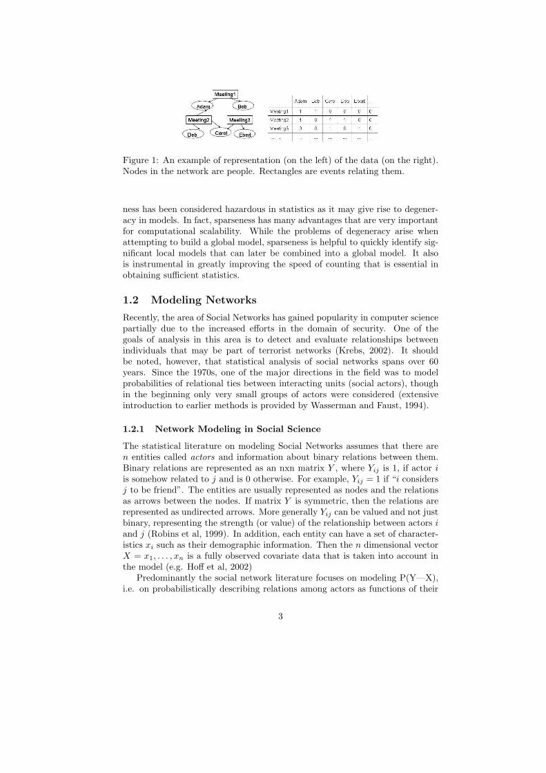
Figure 1: An example of representation (on the left) of the data (on the right).Nodes in the network are people. Rectangles are events relating them.

ness has been considered hazardous in statistics as it may give rise to degener-acy in models. In fact, sparseness has many advantages that are very importantfor computational scalability. While the problems of degeneracy arise whenattempting to build a global model, sparseness is helpful to quickly identify sig-nificant local models that can later be combined into a global model. It alsois instrumental in greatly improving the speed of counting that is essential inobtaining sufficient statistics.

1.2 Modeling Networks

Recently, the area of Social Networks has gained popularity in computer sciencepartially due to the increased efforts in the domain of security. One of thegoals of analysis in this area is to detect and evaluate relationships betweenindividuals that may be part of terrorist networks (Krebs, 2002). It shouldbe noted, however, that statistical analysis of social networks spans over 60years. Since the 1970s, one of the major directions in the field was to modelprobabilities of relational ties between interacting units (social actors), thoughin the beginning only very small groups of actors were considered (extensiveintroduction to earlier methods is provided by Wasserman and Faust, 1994).

1.2.1 Network Modeling in Social Science

The statistical literature on modeling Social Networks assumes that there aren entities called actors and information about binary relations between them.Binary relations are represented as an nxn matrix Y , where Yij is 1, if actor iis somehow related to j and is 0 otherwise. For example, Yij = 1 if “i considersj to be friend”. The entities are usually represented as nodes and the relationsas arrows between the nodes. If matrix Y is symmetric, then the relations arerepresented as undirected arrows. More generally Yij can be valued and not justbinary, representing the strength (or value) of the relationship between actors iand j (Robins et al, 1999). In addition, each entity can have a set of character-istics xi such as their demographic information. Then the n dimensional vectorX = x1, . . . , xn is a fully observed covariate data that is taken into account inthe model (e.g. Hoff et al, 2002)

Predominantly the social network literature focuses on modeling P(Y—X),i.e. on probabilistically describing relations among actors as functions of their

3

covariates and also properties of the graph, such as indegree and outdegree ofindividual nodes. A complete list of graph-specific properties that are beingmodeled can be found in (Snijders et al, 2004). Thus, the models are gearedto probabilistically explain the patterns of observed links and their absencebetween n given entities.

There are several useful properties of the stochastic models listed in a briefsurvey work by Smyth (2003). Some of them are:

• the ability to explain important properties between entities that often oc-cur in real life such as reciprocity, if i is related to j then j is more likelyto be somehow related to i; and transitivity, if i knows j and j knows k,it is likely that i knows k.

• inference methods for handling systematic errors in the measurement oflinks (Butts,2003)

• general approaches for parameter estimation and model comparison usingMarkov Chain Monte Carlo methods (e.g. Snijders, 2002)

• taking into account individual variability (Hoff, 2003) and properties (co-variates) of actors (Hoff,2002)

• ability to handle groups of nodes with equivalent statistical properties(Wang and Wong, 1987).

There are several problems with existing models such as degeneracy, ana-lyzed by Handcock (2003), and scalability, mentioned by several sources (Hoffet al, 2002; Smyth, 2003). The new specifications for the Exponential RandomGraph Models proposed in Snijders et al (2004) attempt to find a solution forthe unstable likelihood by proposing slightly different parametrization of themodels than was used before. Experiments show that the parameters estimatedusing the new approach yield a smoother likelihood surface that is more robustand is less susceptible to the degeneracy problem. The scalability remains to bea major issue. Datasets with hundreds of thousands of entities are not uncom-mon in the Internet and co-authorship based domains. To our knowledge, thereare no statistical models in the social networks literature that would scale tothousands or more actors. Parameter estimation in general for Markov RandomFields is well-known to be intractable for large number of variables due to thecomputational complexity of the normalization constant which requires sum-mation over all possible graphs with n nodes. The scalability problem has alsobeen attributed to the tendency of the models to be global, i.e. most operate onthe full covariance matrices (Hoff et al, 2002). The use of MCMC approachesthat tend to have slow convergence rate may also hinder computational speedof the parameter estimation in high dimensions.

4

One of the more recent directions is latent variable models. Those may beable to avoid the problems related to the use of Markov Random Graphs. Forexample, the work of Hoff et al (2002) proposes a model in which it is assumedthat each actor i has an unknown position zi in a latent space. The links betweenactors in the network are then assumed to be conditionally independent giventhose positions and the probability of a link is a probabilistic function of thosepositions and actors’ covariates. The latent positions are estimated from datausing logistic regression. The general form of the model is:

logodds(yij = 1|zi, zj , xij , α, β) = α + βT xij + d(zi, zj) (1)

where d(zi, zj) is a distance metric between positions of the actors in latentspace. This model is though promising also suffers from the lack of scalabilityof the parameter estimation.

1.2.2 Network Modeling in Physics

It is also worth mentioning that a graph theoretic area of physics that studiescomplex systems is directly applicable to social network modelling. Thoughmodeling of complex systems has developed seemingly in parallel to the sta-tistical modeling of social networks in social science, the findings in this areacan assist in understand further the phenomenon of real networks organizationand structure. The assumptions are the same: there are n actors (nodes) andthere are N links between those nodes representing relationships among actors.The goal is also to understand and model structural properties of the naturallyoccurring networks. The base model describing random graphs was developedby Erdos and Reny (1959), where expected number of edges in the graph isE(N) = p( (n−1)n

2 ), where p is the probability of having any edge, and the prob-

ability of obtaining the observed graph is P (Go) = pN (1−p)n(n−1)

2 −n. However,it was noted that the degree distribution in the random graphs does not followpower law P (k) ∼ k−γ common to the realistic networks. Thus “scale-freenetworks” were introduced (Barabasi and Albert, 1999; Barabasi et al, 1999) .Newman et al (2001) have developed a generalized random graph model wherethe degree distribution is given as an input parameter. The research in the fieldof physics gives more insight into graph growth, given the proposed models,such properties of the emerging graphs as clusterability, graph diameter andthe formation of a large component. A great summary of the past and ongoingwork and its relation to statistical physics is given by Barabasi et al (2002).

1.2.3 Other

A variety of other domains greatly benefit from network analysis. For examplein Biology, motif search in biological networks is facilitated by studying variousgraph properties such as local graph alignment (Berg and Lassig, 2004). Eventhough this work is probabilistic in nature and reveals topological graph proper-ties from the given graph, it is not generative and does not generalize to answer

5

other queries about the data. Friedman (2004) uses probabilistic graphical mod-els to gain insights into biological mechanisms governing cellular networks. Thiswork is probably the closest to ours in its nature. Several assumptions aboutdomain knowledge are used in the constructed models. We make no assump-tions about the structure of the graph underlying the resulting set of events andlearn the dependencies among actors from data directly.

Another work similar in spirit to ours is use of relational dependency net-works RDNs to answer classification queries posed to the network of entities(Neville and Jensen, 2003). Though the network in this case appeared to bequite large (over 300,000 entities), it was considered to be given. McGovern et algives another nice analysis of the high energy physics community based on thecitation graph was done by (McGovern et al, 2003). In this work, graph proper-ties for very large graph of citations (static analysis) was done using sampling.Also, several predictive tasks were tested by learning Relational ProbabilityTrees (Neville et al, 2003) based on featurized data. Again, sampling was usedto train the model resulting in good prediction accuracy. Above work on analyz-ing social communities and learning tasks is based on given network structure,whereas our work is geared to learning that structure. These two directions arecomplementary to each other.

Mapping Knowledge Domains is yet another area that unites physicists, bi-ologist, computer scientists in order to understand the formation of knowledgedomains, their structures and properties. A lot of the work in this area assumesthat a knowledge database can be represented and visualized as a graph struc-ture. The research is geared towards understanding various properties of thedomains, such as topics clustering, number of papers written by authors in singleor across multiple domains, length of the path between actors in co-authorshipnetworks, etc. Methods used to describe those properties and the networks aresimilar in spirit though not always limited to those found in physics literature.A great overview of this work can be found in the special issue of PNAS (April2004) dedicated to this topic.

1.2.4 Network Evolution

One of the important properties of real life networks is evolution over time. Itcan be expected that co-authorship networks can be relatively stable, whereassuch dynamic online communities as Friendster may significantly change in a rel-atively short period of time. In terms of modelling a change in a social network,new interaction means an addition of a new edge, whereas severing a relationshipmeans deletion of an edge. The principles underlying the mechanisms by whichrelationships evolve are still not well understood (Liben-Nowell and Kleinberg,2003). There are several potentially different approaches based on the objectivethe researchers are optimizing. Works of Jin et al (2001), Barabasi et al (2002)and Davidsen (2002) in physics along with Van de Bunt et al (1999) and Huis-man and Snijders (2003) in social sciences, generally evaluate their models fornetwork evolution by comparing structural properties and features of the devel-oped models to those of real networks. Another direction is to model evolution

6

aiming to make inferences, i.e. based on the properties of the network seen sofar, to infer who are the most likely future friends or collaborators (Newman,2001; Liben-Nowell and Kleinberg, 2003). Such models are still in their infancy,having similar problems with scalability and incorporation of secondary factors,such as graduation or relocation that have great impact on real life networks.

1.3 Thesis goals

In my recent work on obtaining scalable models for binary event data, I devel-oped an algorithm for structural search of Bayesian Networks, named Screen-based Bayes Net Structural search (SBNS). Some of the useful properties ofthe algorithm are scalability to over 105 actors while maintaining the ability tosearch pairwise, three-way and higher-order interactions. Experiments showedthat SBNS finds better fitting models than the only available scalable alter-native: random hill-climbing approach. It was also evident that inclusion ofhigh order interactions increased the accuracy. My goals are to examine andimprove on the properties of the SBNS-created-model when applied to socialnetwork domains; to extend the model to incorporate secondary characteristics,i.e. additional information about actors and finally to modify the model to allowevolution over time. I believe that SBNS is a solid framework that could easilyfacilitate further developments to achieve scalable models for social networks.

The rest of this proposal is structured as follows. First, I briefly introducethe existing SBNS model and discuss its benefits and shortcomings and thenelaborate on the exact goals and my plan to achieve them.

2 SBNS model

My initial explorations in the area of large scale graphical models from sparsedata led to the creation of SBNS (Goldenberg and Moore, 2004). SBNS is analgorithm for tractable structural learning of Bayesian Networks in the presenceof sparse event data as described in Section 1.1.

2.1 Bayes Nets

Lets call entities about which the information is collected “actors”. Let’s as-sociate random binary variables Xi, ...Xn with an actor’s participation in anyevent. The state of Xi is 1 when actor i has participated in a given event andis 0 otherwise. For example, for a citation database, if two people i and j haveco-authored a paper together, then for this event (co-authorship of a given pa-per) their states are Xi = 1 and Xj = 1 and the states of all other authors inthe database for this event are 0 (Xk = 0, ∀k 6= i, j).

We would like to learn the underlying dependencies that trigger the events.In other words, based on the known information about simultaneous partici-pation of actors in observed events, we would like to construct a probabilisticgenerative model that would describe those events.

7

A probabilistic model describes a joint over all the random variables of in-terest. Probabilistic graphical models represent joint distributions that can beexpressed as a product of terms each depending on a few random variables. Thegraph provides a dependency structure between variables for each of the termsin the product and is essential in the inference step.

Bayesian Network (BN) is a set {G, θ} where G is a Directed Acyclic Graph{V,E} (V is a set of nodes and E is a set of edges) and θ is a set of parametersobtained by maximizing a Bayesian score, which is usually a penalized likeli-hood. BNs a type of probabilistic graphical model, where the joint distributionis determined by a product of conditional probabilities, i.e.

P (X1 . . . Xn) =∏

i

P (Xi|Pa(Xi)) (2)

, where Pa(Xi) ∈ X is a set of parents of the variable Xi in the DAG. Graphi-cally, BNs are represented using directed edges from parents Pa(Xi) to childrenXi, for each i = 1 . . . n. Acyclicity of the DAG guarantees the product in Equa-tion 2 to be a coherent probability distribution. More information on BayesianNetworks can be found in (Cooper and Herskovitz, 1991; Heckerman et al, 1995).

Note that directed arrows in the graph represent direct dependency of theoutcome of variable Xi on its parents Pa(Xi). Note that the dependenciescan only be described in terms of the observed data, for example in a citationdatabase case, a relation Xi− > Xj , where Pa(Xj) = Xi, means that authorXj is likely to appear as co-author of the paper if Xi is one of the co-authors.The dependence can also represent a negative correlation, i.e. in the above caseknowing that Xi is one of the co-authors, would make Xj unlikely to be one ofthe co-authors.

2.2 Algorithm

The scalability of SBNS is achieved by exhaustively searching over structuresonly on the local level for a large set of small subsets of variables. The advantageof such a structural learning algorithm is that the optimization never needs tobe carried out on the global scale. We exploited the computational efficiency ofFrequent Sets (Agrawal, 1993) for gathering statistics that are most likely to beuseful for structure search given the assumption of sparse data. A Frequent Setwith support s is a collection of variables (entities, actors) that have co-occurred(i.e. simultaneously had 1 in the binary dataset) more than s times. In our workwe show that in sparse data the evidence for positive correlation if such existsis going to be much stronger than for negative one. Given sparse data and asupport s greater than about 3, it is surprisingly easy to compute all FrequentSets (Agrawal, 1994). There is an abundance of literature on Frequent Sets astheir collection is an essential part of the association rules algorithms widelyused in commercial data mining (Agrawal, 1993; Han and Kamber, 2000). Itis important to note that usage of Frequent Sets facilitates finding interactionsof order higher than just dyads and triads, the limitation that still exists inmajority of the Social Networks models. Finally, there is a simple heuristic

8

that iterates over potential edges once, efficiently exploiting locally collectedstatistics and structures to create the global Bayes Net. It was not necessary tomake simplifying assumptions such as restricting the number of possible parentsand thus impacting the structure of the network, since the local searches arequite inexpensive. Pseudocode for the SBNS algorithm is available in Table 1,the detailed explanation of SBNS is available in (Goldenberg and Moore, 2004).

2.3 Advantages of SBNS framework

The main contribution of SBNS is the ability to perform structural search ondatasets such as Citeseer with over 100, 000 variables (authors). Experimentsshow that SBNS finds models fitting the data better than the only scalablealternative, random hill-climbing, on several large datasets including Citeseer.Random hill-climbing is a search algorithm where at each step one of the threeoperations {addition, deletion, reversal} of an edge is applied to the given graph.The modification to the graph is accepted with probability p only if it improvesthe score. The table of results and their analysis are available in (Goldenbergand Moore, 2004). Beyond finding the structure, which carries important infor-mation in itself, we also showed that it was possible to execute certain queriesvery quickly even when the networks are so large. For example, one of thequeries that was reported by Goldenberg and Moore (2004) is similar to all-but-one task in collaborative filtering, where the goal is to find the most likely subsetof variables of given cardinality to complete the given partial set (Heckerman etal, 2000).

The algorithm can be treated as a more general framework. The main ideasthat are useful for scalability of modelling any social network are

1. to be able to identify subsets of actors that

(a) are small enough to allow finding nearly optimal local models opti-mizing the same scoring function quickly

(b) upon local parameter estimation provide a substantial amount ofstatistics (such as counts) necessary for further (global) estimation

2. the model has to be decomposable so that the full joint probability doesnot require estimation of the full covariance matrix

Block models of Wang and Wong (1987) satisfy the first condition, though thesubsets need not be disjoint. The first condition could include soft clusteringinstead of the Frequent Sets, provided condition 1(b) is satisfied. The secondcondition eliminates Markov Random Field (MRF) type models in their presentstate, where the normalization constant has to be computed over all possiblestates of all variables (computationally prohibitive step).

9

algorithm SBNSinput K - max Frequent Set size

s - supportoutput BN - Bayes NetAlso: Ed - Edgedump - a collection of directed edges

represented as (source,dest,count)DS - DAG storage

1. for k = 2 .. K2. obtain counts for all Frequent Sets of size k3. foreach Frequent Set4. find best scoring DAG5. if DAG contains a node that has k−1 par-

ents6. store DAG in DS7. end foreach8. end for9. foreach DAG in DS

10. store all edges {source, dest, count++}in Ed

11. order Ed in decreasing order of edge counts12. foreach edge e ∈ Ed

13. if e doesn’t form a cycle in BN

14. and e improves BDeu15. add e to BN

16. end foreach17. return BN

Table 1: Pseudocode for the SBNS algorithm

10

3 SBNS and Social Networks

I would like to draw a parallel with the Social Network (SN) literature. In theSN paradigm, it is assumed that the links between the actors representing theirrelationships are given. Having the event database, we could also link the actorsbased on their simultaneous participation in an event. However, we observemany events in which actors i, j, k, etc may occur together or separately. Thus,these relations are of probabilistic nature and not considered to be given. It isalso important to note the difference between the ”links” or edges that are foundusing a structural learning algorithm such as SBNS and the ”relationships”between actors. The edges found using SBNS do represent dependency whichhowever cannot be readily interpreted as a relationship in a sense common to SNanalysis. SN relationships can be inferred from a learned Bayes Net by askingquestions such as ”are i and j close collaborators”. One of the ways of answeringthis question would be to find p(Xi|Xk),∀k 6= j and then find whether p(Xi|Xj)is in the desired percentile, such as in the top 5%.

Another difference between the Social Network paradigm and the proba-bilistic graphical model (PGM) as described above is the ability of the PGM tosuccinctly represent the joint distribution, where as the focus of the graphicalmodels commonly used for Social Networks is to fit a model to the existinggraph of relationships as closely as possible. In case of PGMs, one of the goalsis to represent the joint while minimizing the number of parameters used. Thisapproach allows us to handle models with hundreds of thousands of variableswithout running out of memory.

One of the benefits of the commonly accepted models describing social net-works is the possibility of directly assesing the properties of the graph, such asthe number of triangles, k-stars, or degree distribution. It is not possible toanswer the questions about properties using Bayes Nets without a number ofcomplex inference steps. However, though it is hard to create easy visualiza-tions of underlying relationships and draw conclusions from SBNS about theunderlying network itself, we believe that by using inference it is possible tomake judgements about the relationships between actors, one of the ultimategoals of modeling social networks.

4 Example

The purpose of this example is to show similarity and differences in conclusionsthat can be drawn from a social network represented by an adjacency matrixA and a Bayes Net learned using SBNS from the event data that preservesconstraints specified by A.

This illustration is based on a sample dataset borg4cent available in theUCINet package1. The dataset provides a relationship (adjacency) matrix for

1UCINet is a social network analysis package available athttp://www.analytictech.com/ucinet.htm

11

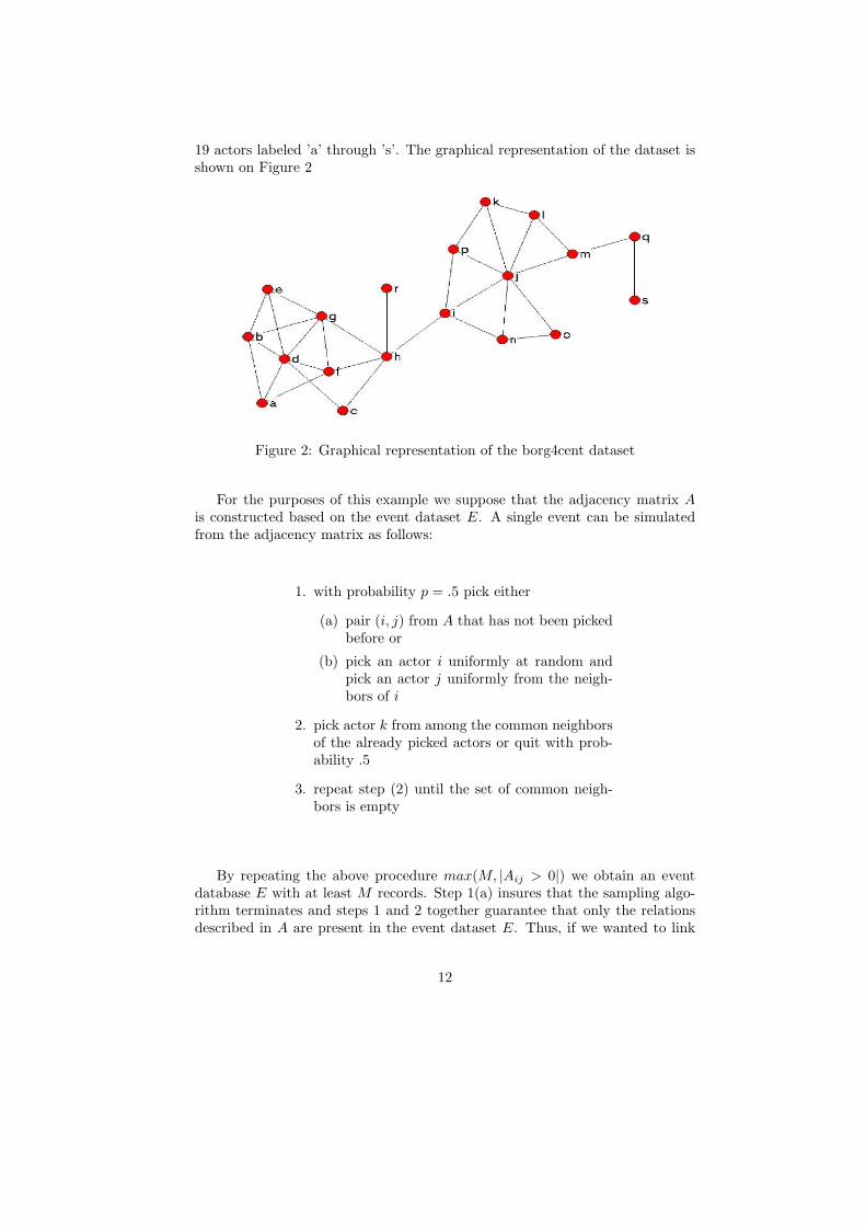
19 actors labeled ’a’ through ’s’. The graphical representation of the dataset isshown on Figure 2

Figure 2: Graphical representation of the borg4cent dataset

For the purposes of this example we suppose that the adjacency matrix Ais constructed based on the event dataset E. A single event can be simulatedfrom the adjacency matrix as follows:

1. with probability p = .5 pick either

(a) pair (i, j) from A that has not been pickedbefore or

(b) pick an actor i uniformly at random andpick an actor j uniformly from the neigh-bors of i

2. pick actor k from among the common neighborsof the already picked actors or quit with prob-ability .5

3. repeat step (2) until the set of common neigh-bors is empty

By repeating the above procedure max(M, |Aij > 0|) we obtain an eventdatabase E with at least M records. Step 1(a) insures that the sampling algo-rithm terminates and steps 1 and 2 together guarantee that only the relationsdescribed in A are present in the event dataset E. Thus, if we wanted to link

12

actors explicitly based on their participation in the events in the simulateddataset, we would obtain graph on Figure 2.

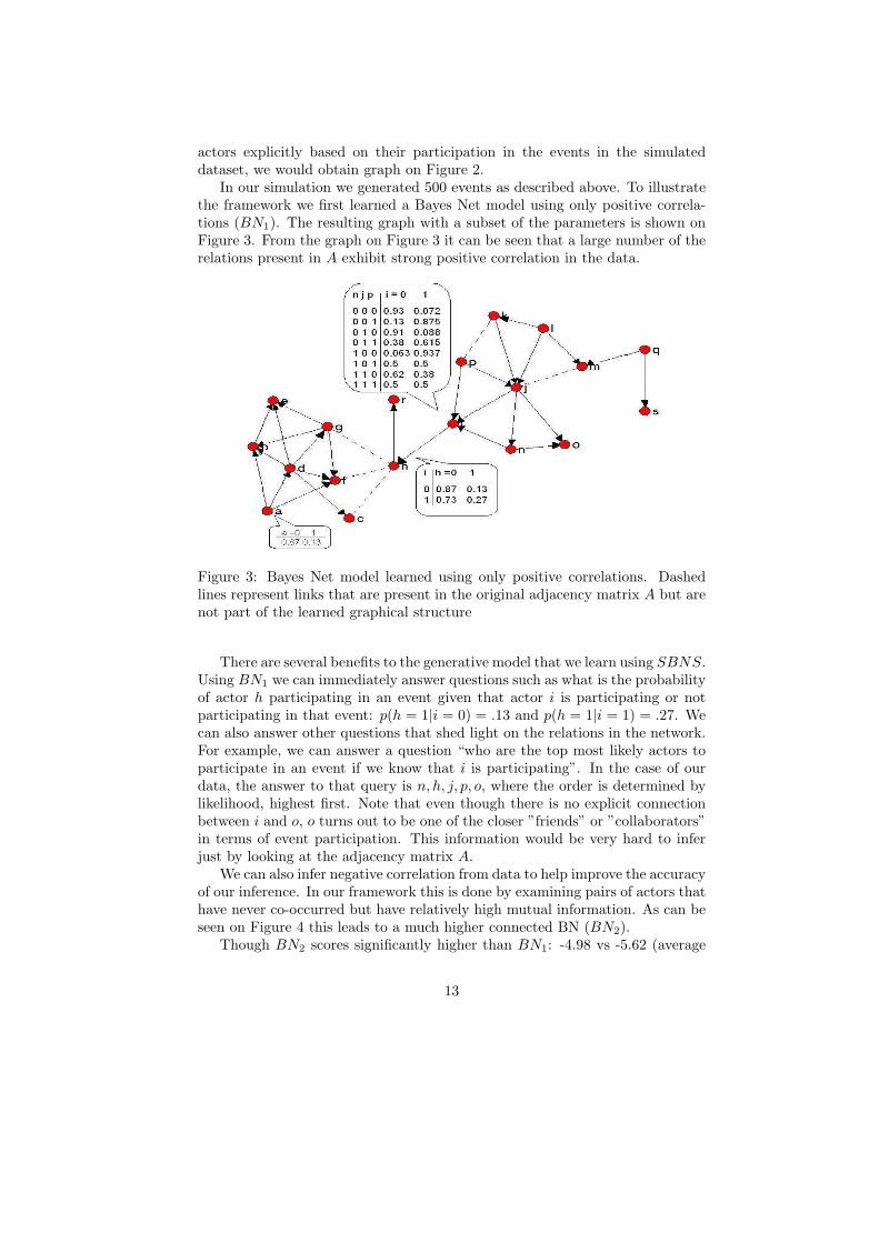
In our simulation we generated 500 events as described above. To illustratethe framework we first learned a Bayes Net model using only positive correla-tions (BN1). The resulting graph with a subset of the parameters is shown onFigure 3. From the graph on Figure 3 it can be seen that a large number of therelations present in A exhibit strong positive correlation in the data.

Figure 3: Bayes Net model learned using only positive correlations. Dashedlines represent links that are present in the original adjacency matrix A but arenot part of the learned graphical structure

There are several benefits to the generative model that we learn using SBNS.Using BN1 we can immediately answer questions such as what is the probabilityof actor h participating in an event given that actor i is participating or notparticipating in that event: p(h = 1|i = 0) = .13 and p(h = 1|i = 1) = .27. Wecan also answer other questions that shed light on the relations in the network.For example, we can answer a question “who are the top most likely actors toparticipate in an event if we know that i is participating”. In the case of ourdata, the answer to that query is n, h, j, p, o, where the order is determined bylikelihood, highest first. Note that even though there is no explicit connectionbetween i and o, o turns out to be one of the closer ”friends” or ”collaborators”in terms of event participation. This information would be very hard to inferjust by looking at the adjacency matrix A.

We can also infer negative correlation from data to help improve the accuracyof our inference. In our framework this is done by examining pairs of actors thathave never co-occurred but have relatively high mutual information. As can beseen on Figure 4 this leads to a much higher connected BN (BN2).

Though BN2 scores significantly higher than BN1: -4.98 vs -5.62 (average

13

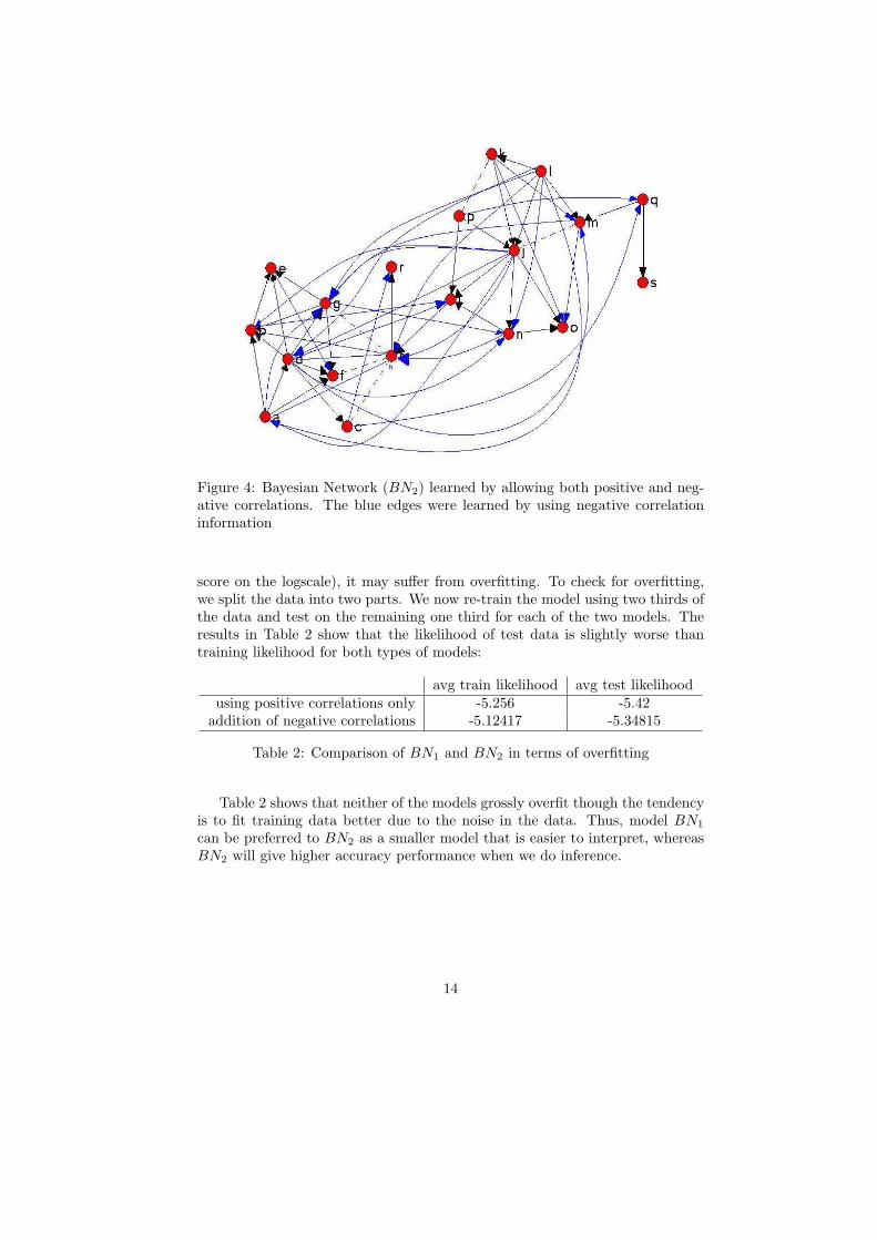
Figure 4: Bayesian Network (BN2) learned by allowing both positive and neg-ative correlations. The blue edges were learned by using negative correlationinformation

score on the logscale), it may suffer from overfitting. To check for overfitting,we split the data into two parts. We now re-train the model using two thirds ofthe data and test on the remaining one third for each of the two models. Theresults in Table 2 show that the likelihood of test data is slightly worse thantraining likelihood for both types of models:

avg train likelihood avg test likelihoodusing positive correlations only -5.256 -5.42

addition of negative correlations -5.12417 -5.34815

Table 2: Comparison of BN1 and BN2 in terms of overfitting

Table 2 shows that neither of the models grossly overfit though the tendencyis to fit training data better due to the noise in the data. Thus, model BN1

can be preferred to BN2 as a smaller model that is easier to interpret, whereasBN2 will give higher accuracy performance when we do inference.

14

5 Proposed work

5.1 Accuracy improvement

Even though the algorithm is scalable to a very large number of actors, it maybenefit from several improvements. Particularly, generating global networksfrom the local models (step 10–16 in the algorithm in Table 1 can be improved.The edges in local structures learned to be added to the global Bayes Nets areordered according to their respective number of occurrences. In case of a tie, theordering is essentially random. It was shown by Friedman and Koller (2003)that ordering is an important factor when building a Bayes Net. One of thesolutions to the ordering problem in our case could be a slightly modified versionof the variable ordering search algorithm developed in collaboration with MaxChickering (Goldenberg and Chickering, 2004). However, ordering algorithmsare computationally expensive. I propose to sample several orders uniformlyat random and learn a Bayes Net corresponding to each of them. The numberof sampled orders depends strictly on the given time constraint which in theworst case should be equal to picking a single random order. To improve thisresult, we can bias our sampling in favor of the orders that seem to have resultedin better Bayes Nets so far. We can afford to sample orders due to the smallcomputational cost of learning a Bayes Net given an order. The computationalbottleneck remains to be counting of the frequencies.

5.2 Types of relationships and undirected models

As was mentioned above, a substantial body of research in Social Networks ex-plicitly models the properties of ties between actors, such as transitivity andreciprocity (Wasserman and Faust, 1994). However, in real life not all relation-ships are reciprocal or transitive, thus the properties can be described betterusing stochastic rather than deterministic models (Snijders, 2004). More re-cently Hoff et al (2002) have proposed a latent space model where, by estimat-ing parameters (latent positions) empirically from data, such properties will beaccounted for automatically.

The SBNS structural search algorithm was not developed with the propertiesof social relationships in mind. However, some of the well known features of thesocial net models still hold. For example, in case of reciprocity, in a dyad xy,if x and y are equally likely then p(y|x) = p(x|y) (according to Bayes Rule).In case of transitivity, if x depends on y and y depends on z, then x and yare almost always unconditionally dependent, even though conditionally theycould be independent (according to factorizations in the Bayes Net). However,we have to be careful about interpreting the graph. If we tried interpreting theedges as relations between actors directly, in cases like co-authorship, where if xand y have co-authored a paper, it might be desired to have an undirected edgebetween them. In a Bayes Net semantics is different. The direction of an edgecan mean, for example “y is more likely given x”, whereas the converse mightnot be true in the data. Still, it is not clear how much we suffer from using

15

acyclic graphs to describe distributions underlying social network phenomena.There are several ways to combat acyclicity in a model. One trivial extension

would be to extend SBNS algorithm to learn Dependency Networks as describedby Heckerman et al (2000). Dependency networks retain the property that eachnode in the network is independent of the other nodes given its parents, whichallows for computationally efficient estimation of parameters. The extension tolearn Dependency Nets using SBNS results in even simpler learning algorithm,where we replace steps 10 − 16 in the algorithm description in Table 1 by glu-ing together local structures from the dag storage DS. However, inference isnot trivial, since not every Dependency Network encodes parsimonious jointdistribution.

It was proved by Heckerman et al (2000) that consistent dependency net-works have equivalent representational power as Markov Random Graphs (MRFs).I am interested in extending SBNS to the undirected graphs. The notion ofobtaining the global model by identifying a set of locally best models wouldtranslate into finding statistically significant cliques. This is easily achievableby finding the best structure for each of the undirected frequent sets by fittingloglinear models using Iterative Proportional Scaling (Bishop et al, 1977). Thenext step would be to glue the cliques together, however this might result in largecycles, which will then cause a problem when estimating the partition function(normalization constant) and doing inference. Extensive research in the MRFsshows that the computational bottleneck is the estimation of the normalizationconstant. Several estimation schemes have been proposed (Ghahramani, 2003),but so far no scalable solutions were found.

5.3 Including actors’ properties

The work by Hoff et al (2002) has shown that the fit of the model improves ifsecondary characteristics (e.g. both actors are the same gender) are taken intoaccount. One of the possibilities is to use secondary information when orderingthe edges in the SBNS algorithm (step 11 in Table 1). In this case, each actorcan be represented as a vector in the space of attributes and in addition to thenumber of occurrences in different local models, each edge could be weighted bythe similarity of the actors participating in it. For example, we could measuresimilarity by the number of attributes that assume the same value for the twoactors. In this case, an edge that does not appear frequently could still outweighfrequent edge if actors of an infrequent dyad are very similar.

The above approach does not take into account actors’ properties whenevaluating local structures. However, it is easy to imagine a situation whereactors’ participation in an event is influenced by their properties. For example,if a given event is a weekly meeting of the Artificial Intelligence lab membersthen it is more likely that students and professors associated with the lab willparticipate in that meeting, rather than students or professors associated witha Computer Architecture lab. In other words, knowing actors’ affiliations canmake their presence in an event more or less likely. Thus, we would ideallylike to incorporate secondary information about actors into the model selection

16

process.I would like to incorporate secondary information regarding actors’ charac-

teristics as priors on the observed frequencies of co-occurrences. Following thesame notation as in Section 2 and in (Heckerman, 1995), let xk

i represent thekth possible state of variable Xi and paj

i , the jth possible state of parents Pai

of the variable Xi. For each variable there are qi states of its parents. Then,for each state of Pai and given local parameterization θi under the model m,p(xk

i |paji , θi) is distributed binomially: p(xk

i |paji , θi) = θijk, where

∑2k=1 θijk = 1

and ∀ijk : θijk > 0. To efficiently calculate the likelihood it is common toassume that θijks are independent and put a Dirichlet prior on the parametersθij :

p(θij) =1

Z(α)

ri∏

k=1

θαijk−1ijk (3)

, where normalization constant is Z(α) =∏ri

k=1Γ(αijk)

Γ(∑ri

k=1αijk)

and parameters α can

be interpreted as ”prior observation counts”. Note that now the structures arenot uniformly probable, so the likelihood, i.e. the model selection criteria, hasa more general form (Heckerman and Chickering, 1996):

p(D|m) =n∏

i=1

qi∏

j=1

Γ(αij)Γ(αij + Nij)

·2∏

k=1

Γ(αijk + Nijk)Γ(αijk)

(4)

, where Nijk are the observed frequencies of the xki given paj

i

There are many ways to calculate prior frequencies from the secondary prop-erties. The simplest way is to empirically estimate αijk from data by counting.Let A be a set of all attributes, which is the same for every variable, and Va

a set of values associated with a particular attribute a. Then the value of theattributes associated with the variable Xi would be vxi

and the value of theparticular attribute of the variable Xi is vaxi

. Also, the set of values of a recordrl is indicated as vrl = {vaxi

: ∀a ∈ A, ∀xi ∈ rl}. To estimate αijk we need tocount the number of records, where the set of values of the attributes of actorsinclude xk

i and paji , i.e. αijk =

∑l rl : vrl ⊃ {vxi

∪ vpai}. If the number of

such records in the dataset is 0, αijk is set to be 1, since parameters of Dirichletare restricted to be positive. In other words, we expect to see as many eventswith the participation of the given actors as there are occurrences of actorswith similar combinations of attribute values. This estimation technique of theDirichlet parameters will increase the likelihood of dependency between actorswith parameter values common in the dataset.

5.4 Inference

To answer questions about how strongly individuals are related and to gain bet-ter insight into the properties of the relationships modeled by Bayes Nets, wehave to do large scale inference quickly. Pavlov and Smyth (2001) have shownthat for a query on a subset of attributes it is more efficient to create a local

17

Bayes Net using only the attributes in the query. The local models in this caseoutperform inference on global Bayes Nets both in efficiency and in accuracy.However, some queries of interest are more global. For example, we might liketo know who are the people that have the most effect on a particular actor. Inthis case, each actor and/or combination of actors could be potential answersto this query. In a graph with 100, 000 or more actors, the most efficient infer-ence techniques applied to the global Bayes Net are computationally infeasible.However, there are assumptions that can be made to speed up the computation.Obviously, no matter how large the graph is, only a handful of actors could bean answer to the query especially if we set the threshold for “significant effect”apriori. Most of the actors in the graph have marginally negligible influence onany given actor. I plan to explore this and other insights and build on some ofthe ideas proposed by Pavlov et al (2003) in order to create a general frameworkfor answering queries that are of interest to social scientists using a global BayesNet.

5.5 Evolution of Social Networks

So far the proposed changes to the model have been static. However, in realdata, especially if it is collected over a long period of time, the relationshipsbetween actors change. For example, in the publication index database, manyof the publications were co-authored by students and their professors. Therelationships and publication patterns tend to change as the students graduate.The model is likely to change significantly in the period of ten years. I would liketo extend my framework to account for the temporal changes in the network.Since Frequent Sets are tuples that occur at least s times, it is conceivable toassume that the changes can be captured locally. For example, when a studentgraduates, the frequency of his/her collaboration with the professor changes. Ifthe change is significant then it will be reflected in all the tuples that contain thestudent and the professor. By monitoring and comparing the global frequenciesof each tuple at time t + 1 to frequencies at time t, it is possible to pinpointthe local models that will need to be re-estimated. Due to the decomposableproperty of the global model, it is possible to localize the re-estimation of thenet and thus incorporate the information about the changes over time in thecomputationally efficient manner.

6 Timeline

The following is the plan to proceed with my research. The tasks are not neces-sarily in the order they will be addressed, since some of them are interrelated.I am budgeting about 25% of each task for evaluation and testing on large realworld datasets.

1. improve SBNS search by modifying the heuristic used to create globalBayes Nets from local ones (Section 5.1) - 2 months

18

2. explore in more depth properties of the models found by SBNS and theirrelation to Social Networks (Section 5.2) - 2 months

3. study algorithms for inference tasks (Section 5.4) - 4 months

4. implement proposed incorporation of the secondary characteristics (Sec-tion 5.3) - 2 months

5. apply variational methods to aid with porting the SBNS idea to the undi-rected graphs (Section 5.2) - 2 months

6. obtain a fitness criteria for undirected graph model selection (Section 5.2)- 3 months

7. evolution of the graph structure over time, possible significant modifica-tion of the model, re-using the same ideas for computational feasibility(Section 5.5) - 5 months

I am hoping to make some advances on each of the above tasks, but in realityone or maybe two tasks may be dropped if they run into serious limitations. I’mplanning to finish proposed research in the next 18-20 months and graduate inAugust of 2006.

References

Agrawal, R., Imielinski, T., & Swami, A. (1993). Mining association rulesbetween sets of items in large databases. ACM SIGMOD 12 (pp. 207–216).

Agrawal, R., & Srikant, R. (1994). Fast algorithms for mining association rules.VLDB 20 (pp. 487–499).

Albert, R., & Barabasi, A.-L. (2002). Statistical mechanics of social networks.Reviews of Modern Physics, 74.

Barabasi, A., Jeong, H., Neda, Z., Ravasz, E., Schubert, A., & Vicsek, T.(2002). Evolution of the social network of scientific collaboration. Physica A,311, 590–614.

Barabasi, A.-L., & Albert, R. (1999). Emergence of scaling in random networks.Science, 286, 509–512.

Barabasi, A.-L., Albert, R., & Jeong, H. (1999). Mean-field theory for scale-freerandom networks. Physica A, 272, 173–187.

19

Berg, J., & Lassig, M. (2004). Local graph alignment and motif search inbiological networks. Proceedings of the National Academy of Science, 101,14689–14694.

Bishop, Y., Fienberg, S., & Holland, P. (1977). Discrete multivariate analysis:Theory and practice. MIT Press.

Breese, J., Heckerman, D., & Kadie, C. (1998). Empirical analysis of predictivealgorithms for collaborative filtering. UAI 14.

Butts, C. (2003). Network inference, error, and informant (in)accuracy: aBayesian approach. Social Networks.

Cooper, G., & Herskovits, E. (1991). A Bayesian method for constructingBayesian belief network from databases. UAI 7 (pp. 86–94).

Davidsen, J., Ebel, J., & Bornholdt, S. (2002). Emergence of a small world fromlocal interactions: Modeling acquaintance networks. Physical Review Letters,88.

Erdos, P., & Reny, A. (1959). On random graphs. Publicationes Mathematicae,6, 290–297.

Frank, O., & Strauss, D. (1984). Markov graphs. Journal of the AmericanStatistical Association, 81, 832–842.

Friedman, N. (2004). Inferring cellular networks using probabilistic graphicalmodels. Science.

Friedman, N., & Koller, D. (2003). Being Bayesian about network structure:A Bayesian approach to structure discovery in Bayesian networks. MachineLearning, 50, 95–125.

Getoor, L., Friedman, N., Koller, D., & Taskar, B. (2002). Learning probabilisticmodels of link structure. Journal of Machine Learning Research.

Ghahramani, Z. (2003). Bayesian learning in undirected graphical models. Talkgiven at the Machine Learning lunch seminar at CMU.

Goldenberg, A., & Chickering, M. (2004). Learning bayesian networks by sam-pling variable orders. Submitted to AISTATS 2005.

Goldenberg, A., & Moore, A. (2004). Tractable learning of large bayes net struc-tures from sparse data. 21st International Conference on Machine Learning.

Han, J., & Kamber, M. (2000). Data mining: Concepts and techniques. MorganKaufmann Publishers.

Handcock, M. (2003). Assessing degeneracy in statistical models of social net-worksWorking Paper 39). University of Washington.

20

Heckerman, D., Chickering, D., Meek, C., Rounthwaite, R., & Kadie, C. (2000).Dependency networks for inference, collaborative filtering, and data visual-ization. Journal of Machine Learning Research, 1, 49–75.

Heckerman, D., Geiger, D., & Chickering, D. (1995). Learning Bayesian Net-works: The combination of knowledge and statistical data. JMLR, 20, 197–243.

Heckerman, D., Meek, C., & Koller, D. (2004). Probabilistic entity-relationshipmodels, prms, and plate models. Proceedings of the 21st International Con-ference on Machine Learning.

Hoff, P. (2003). Random effects models for network data. Proceedings of theNational Academy of Sciences.

Hoff, P., Raftery, A., & Handcock, M. (2002). Latent space approaches tosocial network analysis. Journal of the American Statistical Association, 97,1090–1098.

Huisman, M., & Snijders, T. (2003). Statistical analysis of longitudinal networkdata with changing composition. Sociological Methods and Research, 32, 253–287.

Jensen, J. N. D. (2003). Collective classification with relational dependencynetworks. 9th ACM SIGKDD International Conference on Knowledge Dis-covery and Data Mining. Proceedings of the 2nd Multi-Relational Data MiningWorkshop.

Jin, E., Girvan, M., & Newman, M. (2001). The structure of growing socialnetworks. Physical Review Letters E, 64.

Krebs, V. (2002). Mapping networks of terrorist cells. Connections, 24, 43–52.

Liben-Nowell, D., & Kleinberg, J. (2003). The link prediction problem for socialnetworks. Proc. 12th International Conference on Information and KnowledgeManagement.

McGovern, A., Friedland, L., Hay, M., Gallagher, B., Fast, A., Neville, J., &Jensen, D. (2003). Exploiting relational structure to understand publicationpatterns in high-energy physics. SIGKDD Explorations (pp. 165–173).

Neville, J., Jensen, D., Friedland, L., & Hay, M. (2003). Learning relationalprobability trees. In Ninth ACM SIGKDD International Conference onKnowledge Discovery and Data Mining.

Newman, M. (2001). The structure of scientific collaboration networks. Pro-ceedings of the National Academy of Sciences USA (pp. 404–409).

Pavlov, D., Mannila, H., & Smyth, P. (2003). Beyond independence: proba-bilistic models for query approximation on binary transaction data. IEEETransactions on Knowledge and Data Engineering.

21

Robins, G., Pattison, P., & Wasserman, S. (1999). Logit models and logisticregressions for social networks iii. valued relations. Psychometrika, 64, 371–394.

Smyth, P. (2003). Statistical modeling of graph and network data. IJCAIWorkshop on Learning Statistical Models from Relational Data.

Snijders, T. (2002). Markov chain monte carlo estimation of exponential randomgraph models. Journal of Social Structure, 3.

Snijders, T., Pattison, P., Robins, G., & Handcock, M. (2004). New specifica-tions for exponential random graph models. Submitted for publication.

Van De Bunt, G., Duijin, M. V., & Snijders, T. (1999). Friendship networksthrough time: An actor-oriented dynamic statistical network model. Compu-tation and Mathematical Organization Theory, 5, 167–192.

Wang, Y., & Wong, G. (1987). Stochastic blockmodels for directed graphs.Journal American Statistical Association, 82, 8–19.

Wasserman, S., & Pattison, P. (1996). Logit models and logistic regression forsocial networks: I. an introduction to markov graphs and p∗. Psychometrika,61, 401–425.

22