Properties of magnetic reconnection and FTEs on the ...

manuscript submitted to JGR-Space Physics

Properties of magnetic reconnection and FTEs on the1

dayside magnetopause with and without positive IMF2

Bx component during southward IMF3

S. Hoilijoki1,2, U. Ganse2, D. G. Sibeck3, P. A. Cassak4, L. Turc2, M.4

Battarbee2, R. C. Fear5, X. Blanco-Cano6, A. P. Dimmock7,8, E. K. J.5

Kilpua2, R. Jarvinen7,9, L. Juusola9,2, Y. Pfau-Kempf2, M. Palmroth2,96

1Laboratory for Atmospheric and Space Physics, University of Colorado, Boulder, Colorado, USA7

2Department of Physics, University of Helsinki, Helsinki, Finland8

3NASA Goddard Space Flight Center, Greenbelt, Maryland, USA9

4Department of Physics and Astronomy, West Virginia University, Morgantown, West Virginia, USA10

5Department of Physics & Astronomy, University of Southampton, Southampton, UK11

6Instituto de Geofisica, Universidad Nacional Autonoma de Mexico, Mexico12

7Department of Electronics and Nanoengineering, School of Electrical Engineering, Aalto University,13

Espoo, Finland14

8Swedish Institute of Space Physics, Uppsala, Sweden15

9Finnish Meteorological Institute, Helsinki, Finland16

Key Points:17

• Sunward IMF tilt results in a smaller tangential field at the magnetopause, slow-18

ing dayside reconnection.19

• Smaller tangential field results from a decrease in the IMF component that is shocked20

up at the bow shock.21

• A positive IMF Bx component introduces north-south asymmetries, where fewer22

(but larger) FTEs appear on the southern hemisphere.23

Corresponding author: Sanni Hoilijoki, [email protected]

–1–©2018 American Geophysical Union. All rights reserved.

This article has been accepted for publication and undergone full peer review but has not beenthrough the copyediting, typesetting, pagination and proofreading process which may lead todifferences between this version and the Version of Record. Please cite this article as doi:10.1029/2019JA026821

http://dx.doi.org/10.1029/2019JA026821


Abstract24

This paper describes properties and behavior of magnetic reconnection and flux trans-25

fer events (FTE) on the dayside magnetopause using the global hybrid-Vlasov code Vlasi-26

ator. We investigate two simulation runs with and without a sunward (positive) Bx com-27

ponent of the interplanetary magnetic field (IMF) when the IMF is southward. The runs28

are two-dimensional in real space in the noon-midnight meridional (polar) plane and three-29

dimensional in velocity space. Solar wind input parameters are identical in the two sim-30

ulations with the exception that the IMF is purely southward in one but tilted 45◦ to-31

wards the Sun in the other. In the purely southward case (i.e., without Bx) the mag-32

nitude of the magnetosheath magnetic field component tangential to the magnetopause33

is larger than in the run with a sunward tilt. This is because the shock normal is per-34

pendicular to the IMF at the equatorial plane, whereas in the other run the shock con-35

figuration is oblique and a smaller fraction of the total IMF strength is compressed at36

the shock crossing. Hence the measured average and maximum reconnection rate are larger37

in the purely southward run. The run with tilted IMF also exhibits a north-south asym-38

metry in the tangential magnetic field caused by the different angle between the IMF39

and the bow shock normal north and south of the equator. Greater north-south asym-40

metries are seen in the FTE occurrence rate, size, and velocity as well; FTEs moving to-41

wards the southern hemisphere are larger in size and observed less frequently than FTEs42

in the northern hemisphere.43

1 Introduction44

The solar wind-magnetosphere coupling drives the dynamic evolution of Earth’s45

magnetosphere. Phenomena at the dayside magnetopause associated with the coupling46

impact the entire magnetosphere, including the radiation belts and the magnetotail (e.g.47

Baker, Pulkkinen, Angelopoulos, Baumjohann, & McPherron, 1996; Burton, McPher-48

ron, & Russell, 1975; McPherron, Terasawa, & Nishida, 1986). Magnetic reconnection49

represents the most significant component of the coupling (e.g. Dungey, 1961), which is50

strongest when the interplanetary magnetic field (IMF) is southward (e.g. Akasofu, 1981).51

Consequently, it is important to understand how the nature of reconnection on the mag-52

netopause varies as a function of solar wind conditions.53



Before interacting with the magnetic field of Earth, the solar wind first passes through54

the bow shock and then propagates through the magnetosheath. Reconnection at the55

dayside magnetopause connects magnetosheath magnetic fields to magnetospheric fields.56

Simplified sketches of dayside reconnection often invoke a single quasi-steady reconnec-57

tion site (e.g., Dungey, 1961), but observations suggest that dayside reconnection is of-58

ten bursty, giving rise to FTEs (Russell & Elphic, 1978), which are commonly observed59

at the dayside magnetopause (e.g., Fear et al., 2007; Fear, Palmroth, & Milan, 2012; Kawano60

& Russell, 1997; Rijnbeek, Cowley, Southwood, & Russell, 1984; Wang et al., 2006). Sta-61

tistical surveys find that FTEs form quasi-periodically, on average once every 8 minutes62

(Rijnbeek et al., 1984). Reconnection may occur at single (Fedder, Slinker, Lyon, & Rus-63

sell, 2002; Southwood, Farrugia, & Saunders, 1988) or at multiple reconnection (or X)64

lines (e.g., Lee & Fu, 1985). In the former case, the onset of reconnection results in bubble-65

like magnetic structures (e.g. Southwood et al., 1988), and in the latter case in flux ropes66

of interconnected magnetosheath and magnetospheric magnetic field lines (e.g., Lee &67

Fu, 1985). The scale sizes for FTE flux rope diameters can reach 1-2 RE (e.g., Fear et68

al., 2007; Rijnbeek et al., 1984), while dimensions along the X line can be considerably69

longer (e.g., Fear et al., 2008). Recently, with the high resolution observations provided70

by the Magnetospheric Multiscale (MMS) mission (Burch, Moore, Torbert, & Giles, 2016)71

many smaller ion scale flux rope structures have been observed (e.g., Dong et al., 2017;72

Eastwood et al., 2016; Zhong et al., 2018).73

The north/south IMF Bz component is an important parameter controlling the over-74

all reconnection rate (e.g., Vasyliunas, 1975), and it also impacts the formation and prop-75

erties of the FTEs (e.g., Berchem & Russell, 1984; Rijnbeek et al., 1984; Wang et al., 2006).76

Berchem and Russell (1984) analyzed five years of ISEE observations and found that FTEs77

on the dayside tend to occur during southward IMF with only a few FTEs observed dur-78

ing slightly northward IMF. Wang et al. (2006) used three years of Cluster observations79

to show that IMF Bz impacts the peak-to-peak magnitudes (measured as the absolute80

difference between the bipolar peaks in the magnetic field component BN normal to the81

magnetopause) and separation time between consecutive FTEs, with the separation time82

growing with increasing IMF Bz. For the present study, we focus on the orientation of83

the IMF when it has a negative (southward) Bz component.84

Other factors may also control the nature and effectiveness of reconnection and FTEs85

on the dayside magnetopause. Both observations and simulations have been used to study86



the effects of the IMF clock angle, θ = arctan(By/Bz), where By/Bz is the ratio be-87

tween the IMF y (opposite Earth’s motion around the Sun) and z (normal to the eclip-88

tic) components, on the distribution of FTEs and the location of X lines (e.g., Fear et89

al., 2012; Karlson, Øieroset, Moen, & Sandholt, 1996; Kawano & Russell, 1997). How-90

ever, the influence of the sunward Bx component on FTE formation has not been as thor-91

oughly investigated. Wang et al. (2006) reported that Bx controls the occurrence of FTEs92

but not the separation time or peak-to-peak magnitude of FTEs. They reported that93

more FTEs were observed during positive than negative IMF Bx. A statistical study us-94

ing Time History of Events and Macroscale Interactions during Substorms (THEMIS)95

mission (Angelopoulos, 2008) observations and studies using global magnetohydrody-96

namic (MHD) simulations show that the X line shifts northward for sunward directed97

Bx and southward for antisunward Bx (Hoilijoki, Souza, Walsh, Janhunen, & Palmroth,98

2014; Hoshi, Hasegawa, Kitamura, Saito, & Angelopoulos, 2018; Peng, Wang, & Hu, 2010).99

This study employs the hybrid-Vlasov code Vlasiator for the global magnetosphere100

(Palmroth, Ganse, et al., 2018; von Alfthan et al., 2014, http://www.helsinki.fi/vlasiator).101

In the present paper simulations are global and two-dimensional in real space and three-102

dimensional in velocity space (2D-3V). For simplicity, we consider systems without a dipole103

tilt and with steady solar wind conditions. We compare simulation results for two cases104

with the same total magnetic field strength, but with different IMF tilt. In the first sim-105

ulation the IMF is purely southward, and in the second simulation the IMF is tilted sun-106

ward by 45◦. We find that the average reconnection rate is lower in the run with the sun-107

ward IMF Bx component due to the smaller tangential magnetic field magnitude in the108

magnetosheath. The tilt in the IMF direction also introduces north-south asymmetries109

in the observed properties of the FTEs, including occurrence rate, sizes of the FTEs, and110

their velocities.111

This paper is organized as follows. The details of the simulations and their setup112

are presented in Sec. 2. The data analysis and results are shown in Sec. 3. Finally, we113

discuss the results and provide concluding remarks in Sec. 4.114

2 Simulation Setup115

The simulations employ the Vlasiator global magnetospheric hybrid-Vlasov code116

(Palmroth et al., 2015; Palmroth, Ganse, et al., 2018; von Alfthan et al., 2014), where117



ions evolve as distribution functions in three velocity-space dimensions and electrons are118

treated as a massless fluid described by the generalized Ohm’s law including the Hall term.119

The simulations are two-dimensional in ordinary space and confined to the noon-midnight120

meridional plane. The simulation using a purely southward IMF condition, referred to121

as Run A, is the same simulation discussed by Hoilijoki et al. (2017), Palmroth et al. (2017),122

Jarvinen et al. (2018), and Juusola et al. (2018), with a domain extending from −94 to123

+48RE in the x direction and from −56 to 56RE in the z direction, where RE is Earth’s124

radius and we use geocentric solar ecliptic (GSE) coordinates in which x points sunward,125

y points opposite Earth’s motion about the Sun, and z points normal to the ecliptic plane.126

The simulation with a sunward tilted IMF, referred as Run B, has the same initial con-127

ditions except that the IMF is tilted sunward by 45◦ so that the magnitudes of the x and128

z components of the magnetic field are equal. The simulation domain for Run B spans129

−48 to +64RE in x and −59 to 39RE in the z direction to accommodate the foreshock130

that forms upstream from the south part of the bow shock. Run B produces cavitons131

and spontaneous hot flow anomalies in the foreshock, which are analyzed in a separate132

study (Blanco-Cano et al., 2018).133

Solar wind parameters at the sunward boundary in x are held steady, including a134

fast solar wind with velocity of −750 km/s in the x direction, a density of n = 1 cm−3,135

a proton temperature of Tp = 0.5 MK with a Maxwellian distribution, and a magnetic136

field of magnitude 5 nT, meaning that in Run A the magnetic field components are Bx =137

0 and Bz = −5 nT and in Run B they are Bx = 3.54 nT and Bz = −3.54 nT. We138

point out that the goal of this study is to investigate the fundamental properties of FTEs139

and reconnection at the dayside magnetopause, so we do not attempt to simulate a mag-140

netosphere with commonly observed properties; we do not believe the results of this study141

are adversely impacted by the chosen solar wind parameters. The other three outer bound-142

aries of the simulation domain apply a copy condition, i.e., the magnetic field and the143

velocity distribution function are copied from the closest simulation spatial cells to the144

boundary cell allowing a smooth outflow. The out-of-plane direction has a periodic bound-145

ary condition. The inner boundary with a radius of 5RE is an ideal conducting sphere.146

The grid resolution is 300 km in ordinary space and 30 km/s in velocity space.147

Run A is carried out for t = 2150 seconds of simulation time while Run B is car-148

ried out for t = 1437 seconds. The simulations are initialized slightly differently. Ini-149

tially both simulations set the solar wind density and velocity throughout the whole sim-150



ulation domain and employ a 2-D line-dipole with a strength resulting in a magnetopause151

standoff distance comparable to that of Earth’s dipole, with a corresponding mirror dipole152

outside the solar wind inflow boundary. Details on the line dipole approach were described153

by Daldorff et al. (2014). The difference is that in Run A, the only magnetic field com-154

ponent initially in the simulation domain is that of the dipole field, while the IMF en-155

ters from the inflow boundary and pushes the dipole field to form the magnetosphere.156

In Run B, in addition to the dipole field, the IMF is also initially set throughout the whole157

simulations domain to preserve the solenoidality of the magnetic field in the presence of158

a non-zero IMF Bx component. Therefore, the reconnection at the dayside magnetopause159

becomes properly initialized earlier in Run B than in Run A; this does not impact the160

results of the study. We analyze the time period from 1250 s to 1975 s for Run A and from161

900 s to 1437 s for Run B.162

3 Results163

During the steady solar wind conditions, multiple FTEs occur in both Runs A and164

B as can be seen in Movie S1 in the supporting information. Figure 1 shows a sample165

time slice (t = 1200 s) of the structure of the dayside magnetosphere and magnetosheath166

for each simulation. Here the color indicates the ion temperature and magnetic field lines167

are overlaid so that the magnetic flux interval between consecutive magnetic field lines168

is the same in both panels. Panels (a) and (b) show, respectively, Run A (purely south-169

ward IMF simulation) and Run B (the simulation with sunward IMF tilt). In these sim-170

ulations with only two spatial dimensions, FTEs appear in the form of closed magnetic171

islands. In panel (a) the two largest FTEs are located at x = 8 RE and z = ±3 RE172

and in panel (b) one large FTE is visible at x = 9RE , z = −1RE . Both simulations173

also exhibit a number of smaller FTEs with a range of sizes, including some too small174

to see in Figure 1.175

3.1 Bow shock location and tangential magnetic field179

In both simulations, for the chosen strength of the line dipole moment, the equa-180

torial dayside magnetopause lies approximately at 8 RE from Earth. In Run A the bow181

shock is symmetric and extends up to 19 RE from Earth on the dayside. Run B, with182

the IMF tilted towards the Sun, has a north-south asymmetry in the bow shock shape183

due to the foreshock and quasi-parallel bow shock in the south while the nose of the bow184



Figure 1. Overview plot showing the ion temperature with magnetic field lines overlaid for

(a) Run A, the purely southward IMF simulation and (b) Run B, the southward IMF with 45◦

sunward tilt. The time plotted is t = 1200 s for both simulations.

176

177

178

shock lies at 16 RE . The extent of the quasi-perpendicular magnetosheath becomes larger185

than the quasi-parallel, which is consistent with theory and previous findings (e.g. Chap-186

man & Cairns, 2003; Lin, Swift, & Lee, 1996; Turc, Fontaine, Savoini, & Modolo, 2015).187

According to the Merka, Szabo, Slavin, and Peredo (2005) bow shock model for the same188

upstream conditions as used in the simulation runs, Earth’s subsolar bow shock is pre-189

dicted to be located approximately at 15 RE in both cases. The larger stand-off distance190

of the bow shock in the simulations compared to the model is caused by the two-dimensionality191

of the simulation domain as the magnetic field and plasma can flow around the Earth192

only in the simulation plane and, therefore, pile on the dayside magnetosheath. How-193

ever, the large extent of the magnetosheath in the simulation does not affect the local194

physics that occur at the bow shock, in the magnetosheath and at the magnetopause.195

Vlasiator simulations have been found to reproduce observed features of the foreshock196

velocity distributions and waves (Kempf et al., 2015; Palmroth et al., 2015; Pfau-Kempf197

et al., 2016; Turc et al., 2018), foreshock transients (Blanco-Cano et al., 2018), magne-198

tosheath mirror mode waves (Hoilijoki et al., 2016) and high-speed jets (Palmroth, Hi-199

etala, et al., 2018), and reconnection rates at the dayside magnetopause (Hoilijoki et al.,200

2017).201



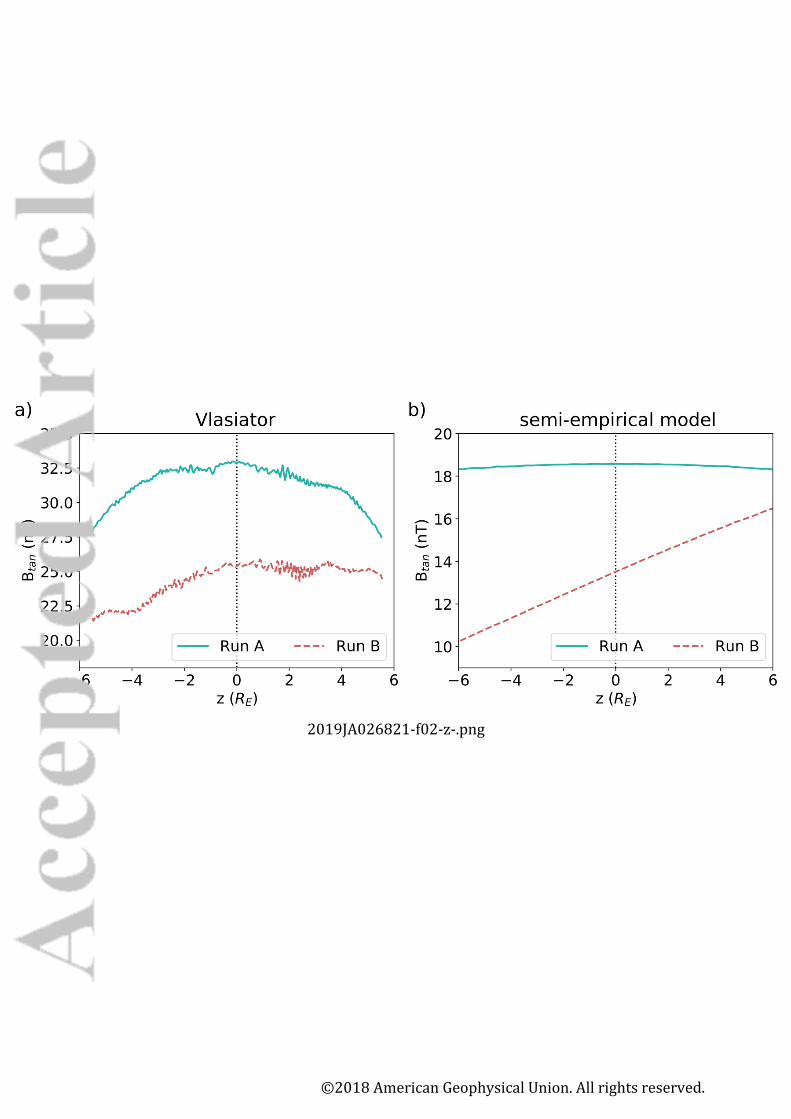
The magnetic field lines plotted in Figure 1 demonstrate that the magnetic field202

magnitude in the magnetosheath is smaller in Run B than in Run A. Figure 2a shows203

the average value of the magnitude of the magnetic field component tangential to the204

magnetopause Btan measured at a distance of 3 RE further outward into the magnetosheath205

to avoid the impact of the passing FTEs on the magnetic field. In Run A, Btan is rel-206

atively symmetric between the northern and southern hemispheres, and at the subso-207

lar point the magnitude is almost 7 nT larger than in Run B. On the contrary, in Run208

B Btan is larger in the northern hemisphere than in the southern one.209

For comparison, we estimate the magnetosheath magnetic field component tangen-210

tial to the magnetopause at the same distance from this boundary as in Vlasiator us-211

ing a semi-empirical model of the magnetosheath magnetic field based on ideal MHD (Turc,212

Fontaine, Savoini, & Kilpua, 2014) shown in Figure 2b. We use as inputs to the model213

the upstream conditions of the two Vlasiator runs. The magnetic field just downstream214

of the bow shock is computed based on Rankine-Hugoniot relations, and it is then prop-215

agated into the magnetosheath using ideal MHD equations. A full description of the model216

is given by Turc et al. (2014). While the model initially employed the Jerab, Nemecek,217

Safrankova, Jelınek, and Merka (2005) bow shock model to estimate the position and218

shape of this boundary, because it was more reliable for the low Mach number conditions219

under study in Turc et al. (2014), we use here the Merka et al. (2005) bow shock model,220

better suited to the upstream conditions in the Vlasiator simulations. Also, as in Turc,221

Fontaine, Escoubet, Kilpua, and Dimmock (2017), the magnetic field compression ra-222

tio is calculated using the Borovsky (2013) formula. The behaviour of the tangential mag-223

netic field component given by the semi-empirical model is similar to that in Vlasiator.224

In the purely southward case Btan is largest at the equatorial plane and symmetric be-225

tween north and south whereas in the tilted IMF case Btan is smaller and asymmetric226

increasing from south to north. Due to the magnetic field pile up caused by the two-dimensionality227

of the simulations, the magnitude of Btan in Vlasiator simulations is larger than that given228

by the semi-empirical model.229

In Run A, the IMF is southward so that at the subsolar point the angle θBn be-233

tween the IMF and bow shock normal is 90◦, i.e., the shock is perpendicular and the mag-234

netic field compression at the bow shock is highest. At higher latitudes, θBn decreases,235

meaning that the IMF component normal to the bow shock increases, but the change236

is symmetric between the north and south. The magnetic field component normal to the237



Figure 2. Average magnitude of the tangential magnetic field component from a distance of

3 RE from the magnetopause from a) Vlasiator simulations and b) a semi-empirical model based

on MHD.

230

231

232

shock is conserved in the shock crossing and only the tangential component is compressed238

(e.g., Treumann, 2009). Therefore, the tangential magnetic field in the magnetosheath239

diminishes at higher latitudes. Because of the sunward tilt in the IMF in Run B, the bow240

shock is quasi-parallel to the south and quasi-perpendicular to the north of the equator.241

At the equatorial plane θBn = 45◦, only the IMF Bz component is compressed. Con-242

sequently, the magnetosheath magnetic field is weaker than in Run A. Also, in the south-243

ern hemisphere in the quasi-parallel magnetosheath the tangential magnetic field is smaller244

than in the northern hemisphere behind the quasi-perpendicular bow shock where a larger245

fraction of the IMF is compressed. Therefore, our simulations show that, despite the IMF246

draping around the magnetopause, the tilt in the IMF orientation causes differences in247

the magnitude of the magnetosheath magnetic field. This is important because the tan-248

gential component of the magnetic field is the component that participates in magnetic249

reconnection at the magnetopause.250

3.2 Reconnection Rates251

Using the method of flux functions described in Appendix A, we locate magnetic252

field X and O points, that represent the reconnection points and the centers of magnetic253

islands (i.e., 2D representations of FTEs), respectively. At each X point, we measure the254

reconnection rate as the out-of-plane component of the electric field Ey. Figure 3 shows255

the probability distributions of reconnection rates at X lines located between z = ±4256

RE from both simulations. The distribution of the reconnection rates in Run A is broader257



Figure 3. Normalized distribution of the reconnection rate Ey at X lines located between

z = ±4 RE and the mean reconnection rate (dashed line) in (a) Run A with mean at 2.9 mV/m

and (b) Run B with mean at 2.1 mV/m.

275

276

277

and reaches higher reconnection rates (above 6 mV/m). The average reconnection rate258

is 2.9±1.2 mV/m (dashed line in Fig. 3a) and the median is 2.8 mV/m. In Run B, the259

peak is steeper and the maximum reconnection rate is lower (∼ 5 mV/m) than in Run260

A. Both the average and median values of the reconnection rate are 2.1±0.9 mV/m in261

Run B (dashed line in Fig. 3b).262

The smaller reconnection rate in Run B is a consequence of the smaller tangential263

magnetic field in magnetosheath caused by the sunward IMF component discussed above.264

To see this, note that for θBn, the southward component of the field is 1/√

2 ≈ 0.707265

as big as it is for the due southward IMF case. The reconnection rate scales approximately266

as [B3/2sh Bms/(Bsh+Bms)

1/2]/√µ0ρsh (Cassak & Shay, 2007), where Bsh and Bms are267

the magnetosheath and magnetosphere reconnecting magnetic field strengths, ρsh is the268

magnetosheath density, and the magnetospheric density is assumed to be negligible. Us-269

ing Bms ' 60 nT and Bsh decreasing from 32.5 nT to 25 nT, one finds that the recon-270

nection rate decreases to approximately 70% of its due southward value. Note, 70% of271

2.9 mV/m is 2.04 mV/m, in excellent agreement with the measured value of 2.1 mV/m.272

This suggests that the decrease in reconnection rate is due to the decrease in the strength273

of the reconnecting component of the magnetosheath magnetic field.274

3.3 North-South asymmetry of FTEs278

Next, we study the probability of encountering an individual FTE at different lo-279

cations along the dayside magnetopause. In order to do so we need to identify the lo-280



Figure 4. Distribution of number of FTEs observed in 1 minute within one 1 RE bins along

the dayside magnetopause in (a) Run A and (b) Run B. The horizontal axis shows the z coor-

dinate along the magnetopause. The vertical dotted line in both panel depicts the equatorial

plane.

290

291

292

293

cations of each X point and O point (regarded as the centers of FTEs) at every time step,281

which we do using the flux function method described in Appendix A. Figures 4a and282

b illustrate the distribution of FTEs passing each point on the magnetopause (divided283

into 1 RE bins) per minute from Run A and Run B, respectively. In Run A the FTE284

occurrence rate in both hemispheres and in the subsolar region is quite flat at ∼ 1.7 FTEs/min285

(except for a small peak at z ∼ +3RE) and, therefore, the chance of encountering FTEs286

does not depend on the hemisphere. In Run B, however, the rate of FTE encounters in287

the northern hemisphere is twice as large as in the southern hemisphere. This shows that288

the IMF Bx component causes a north-south asymmetry in the occurrence rate of FTEs.289

It is also interesting to see if the sunward tilt in the IMF has an impact on FTE294

sizes and their evolution versus latitude. We calculate the enclosed area of the FTEs us-295

ing the method described in Appendix B. Figure 5 shows the z coordinate of the FTE296

locations on the magnetopause plotted as a function of time for both simulations. The297

color and the area of the circle marking the location of each FTE are proportional to the298

cross-sectional area enclosed by the last closed field line of the FTE. The results show299

that the size of most of the FTEs increases as they move to higher latitudes. Some of300

the FTEs in Run A reach a cross sectional area of 5R2E both north and south of the equa-301

tor. These are the ones that spend longer times near the subsolar region before travel-302

ing poleward (Ku & Sibeck, 1998). There is a clear north-south asymmetry in the FTE303

enclosed area for Run B compared to Run A. In particular, the FTEs propagating north-304



-6

-4

-2

0

2

4

6

1200 1300 1400 1500 1600 1700 1800 1900

a)

GSE z

(R

E)

Time (seconds)

-6

-4

-2

0

2

4

6

900 1000 1100 1200 1300 1400

b)

GSE z

(R

E)

Time (seconds)

0

0.5

1

1.5

2

2.5

3

3.5

4

4.5

FTE A

rea (

RE

2)

Figure 5. Location of the FTEs, color coded with the enclosed area. The area of the circles is

proportional to the area of the closed field lines in (a) Run A and (b) Run B.

307

308

ward in Run B remain relatively small whereas in the south there are fewer FTEs, but305

two of them reach an enclosed area over 4.5R2E , larger than is typical in Run A.306

Figure 6a presents the dependence of FTE size on FTE location. Using the calcu-309

lated enclosed area of each FTE and assuming a circular cross-section, we estimate the310

average radius of the FTEs and plot it as a function of z coordinate in Fig. 6a. In Run311

A, the average radius of the FTEs is close to ∼ 1500 km ≈ 10 di (ion inertial length312

di ≈ 150 km in the magnetosheath in the vicinity of the magnetopause in this simu-313

lation) near to the subsolar region. The region of smaller radius FTEs (r < 2000 km),314

i.e. the region where they are generated, is slightly shifted northward from the subso-315

lar region, residing between z = −1 RE and 3 RE . The average radius both in the south-316

ern and northern hemisphere approaches ∼ 2750 km (≈ 18 di) at higher latitudes. The317

FTEs keep growing after formation due to ongoing reconnection at the X lines encom-318

passing the FTE. In the simulations FTE sizes also increase as they coalesce with other319

FTEs (e.g., Akhavan-Tafti et al., 2018; Finn & Kaw, 1977; Hoilijoki et al., 2017; Omidi,320

Blanco-Cano, Russell, & Karimabadi, 2006). The FTE sizes exhibit more north-south321

asymmetry in Run B. The region where the FTEs are generated and their radius is small322



Figure 6. a) Average radius of the FTEs at different points along the magnetopause as a

function of z. b) Average velocity of the FTEs as a function of z from both runs. The vertical

dashed line depicts the equator.

332

333

334

lies between z = 1 RE and 4 RE . On average the FTEs in the southern hemisphere grow323

larger than in the northern hemisphere because they form north of the equator and travel324

further along the magnetopause and therefore have a longer time to process flux through325

reconnection and coalesce with other FTEs. Statistical spacecraft studies have also shown326

that the FTEs observed near the subsolar region, which have an average radius of 15 di,327

are 3 to 7 times smaller than FTEs observed at higher latitudes (Akhavan-Tafti et al.,328

2018; Fermo, Drake, Swisdak, & Hwang, 2011; Wang et al., 2005). Our results suggest329

that the FTE radius roughly doubles from ∼ 10 di in the subsolar region to almost ∼330

20 di around z = 7RE , which is consistent with the observations.331

We calculate FTE velocities as the first order time derivative of the O point loca-335

tions as they propagate along the magnetopause. The results are plotted for both IMF336

cases averaged over 1 RE bins in the z direction in Figure 6b. In Run A (shown in cyan337

boxes), the profile of the average FTE velocities is broadly symmetric in both hemispheres.338

In Run B (shown in red circles), the FTEs propagating towards the northern cusp have339

larger velocities than those moving southward. FTEs propagate along the magnetopause340

as solid bodies having the same velocity as the plasma bulk velocity at the core of the341

FTEs. We suggest that as FTEs north of the equator are smaller, containing also less342

plasma, they require less force to accelerate to higher velocities than the larger FTEs on343

the southern hemisphere. In addition, the FTEs with the purely southward IMF are gen-344

erally faster at the same latitude than the FTEs in the simulation with positive IMF Bx.345

It is possible that in Run A the faster outflow reconnection jet velocities that are caused346



by higher tangential magnetic field, vout,2 ∼ 0.84vout,1 (Cassak & Shay, 2007), push the347

FTEs and cause them to accelerate faster to higher velocities.348

4 Discussion and Conclusions349

This study describes properties of dayside magnetopause reconnection and FTEs350

in two global hybrid-Vlasov Vlasiator simulations. The only difference in the solar wind351

input values used for the two simulations is the orientation of the IMF. Run A has a purely352

southward IMF, whereas Run B has an IMF tilted 45◦ sunward, so that the magnitude353

of the southward Bz component is smaller and Bx is nonzero and positive. We find that354

even though the magnitude of the IMF is the same in both simulations, the magnetic355

field tangential to the magnetopause measured in the magnetosheath is smaller and has356

a north-south asymmetry in the simulation with sunward IMF component. These are357

caused by the different angle between the shock normal and IMF θBn. When θBn = 90◦,358

the IMF is strictly perpendicular to the bow shock and the magnetic field compression359

is highest at the shock crossing, which is the case at the nose of the bow shock in Run360

A with purely southward IMF. In Run B, with tilted IMF, the IMF component tangen-361

tial to the bow shock is larger in the north and smaller in the south causing a north-south362

asymmetry in the magnetic field magnitude downstream of the shock. Because the day-363

side reconnection rate depends on the local tangential magnetic field (e.g. Cassak & Shay,364

2007) the estimated reconnection rates at the X line locations on the dayside magnetopause365

in Run A exhibit a higher maximum and average rate than in Run B.366

Some of the existing coupling functions that determine the reconnection rate at the367

magnetopause as a function of solar wind parameters include the effects of the clock an-368

gle between B and the z axis in the yz plane (e.g. Borovsky, 2013) but not the effect of369

the oblique θBn in the xz plane that could cause a significant north-south asymmetry370

in the tangential magnetic field close to the magnetopause. A reconnection rate value371

calculated for the θBn at the subsolar point or using only the IMF Bz component might372

not give an accurate description of the reconnection rate at an X line that is located north373

or south from the equator, suggesting that the effect of the sunward tilt needs to be in-374

corporated at all latitudes to accurately predict the reconnection rates.375

The north-south asymmetries introduced by the sunward tilt of the IMF suggest376

that the X line resides north of the equatorial plane for a longer period of time than in377



the strictly southward IMF run. The shift of the X line towards the northern hemisphere378

with positive IMF Bx component has been observed before in a statistical THEMIS study379

(Hoshi et al., 2018) and global MHD simulations (Hoilijoki et al., 2014; Peng et al., 2010).380

Often the shift of the X line is explained using the maximum magnetic shear model (Trat-381

tner, Mulcock, Petrinec, & Fuselier, 2007; Trattner, Petrinec, Fuselier, & Phan, 2012),382

but in this case without an out-of-plane magnetic field By component the shear is the383

same everywhere along the magnetopause and, therefore, cannot explain the shift. A model384

based on maximization of a reconnection related parameter that is dependent on Btan,385

for example the outflow velocity (Swisdak & Drake, 2007) or reconnection rate (Borovsky,386

2013), could provide a more likely explanation for the shift of the X line location in these387

simulations.388

Using three years of Cluster observations, Wang et al. (2006) investigated the in-389

fluence of solar wind parameters, including different components of the IMF, on FTE390

properties. The IMF Bz was found to be an important driver for almost all FTE attributes391

but the authors also found some dependencies on Bx. In particular, they found that FTE392

occurrence rates depend on both these IMF components. Our results show that the IMF393

tilt (positive Bx) has an impact on properties of FTEs in both the northern and south-394

ern hemispheres. The comparison of the occurrence rate at different latitudes in both395

simulations show that the positive IMF Bx component increases the probability of en-396

countering an FTE on the northern hemisphere and decreases it on the southern hemi-397

sphere compared to the purely southward IMF case. The total FTE occurrence rate is398

higher in Run A with purely southward IMF, i.e., larger southward IMF component and399

Bx = 0. Statistics by Wang et al. (2006) show a peak in the occurrence around Bz =400

−3 nT and an increasing occurrence rate with increasing IMF Bx. However, our results401

suggest that the effect of the IMF Bx on the occurrence rate depends on where the ob-402

server is located. In the northern hemisphere the observer would see an increased occur-403

rence rate and in the southern hemisphere a decreased rate compared to the case with-404

out the IMF Bx component.405

Figure 5 suggests that FTEs evolve differently northward and southward of the main406

X line when it is located away from the subsolar point. There are many more small FTEs407

on the higher latitude side of the X line, when the X line itself is not located at the equa-408

tor. Events generated at higher latitude move in the same direction as the background409

magnetosheath flow and leave the dayside region quickly without growing to large sizes.410



Some of the events generated closer to the equator move opposite to the magnetosheath411

flow and have more time to grow through reconnection and coalescence to larger sizes.412

This explains, at least partly, the north-south asymmetry in the occurrence rate, size and413

velocity distributions. Similar behavior for FTEs was reported by Ku and Sibeck (1998)414

who used a 2D single X line MHD model. They showed that FTEs moving in the direc-415

tion of the magnetosheath flow accelerate, reducing the duration over which they can416

be observed. The velocity of FTEs moving opposite to the magnetosheath flow decreases,417

causing the event duration to become longer.418

In conclusion, tilting a southward IMF so that it has a sunward component results419

in a smaller magnitude of the tangential magnetic field with north-south asymmetries420

in the magnetosheath close to the magnetopause due to the different angle between the421

IMF and the bow shock normal. Because the tangential field is smaller, the dayside re-422

connection rate is smaller as well. In addition, the tilt in the IMF causes a north-south423

asymmetry in properties of FTEs, including occurrence rate, size and velocity that are424

not present in the simulation with a purely southward IMF orientation. Our results sug-425

gest, as a consequence of rotating the IMF to have a positive Bx component, that the426

FTEs on the northern hemisphere occur more frequently, are smaller, and accelerate faster427

than FTEs on the southern hemisphere.428

A X and O point location calculations429

We locate reconnection X lines (points in 2D) and O points (FTEs) using a stan-430

dard approach in 2D simulations. We calculate the magnetic flux function ψ(r, t),431

ψ(r, t) =

(∫ r

r0

B(r, t)× dl)

y

, (A.1)

where B is the vector magnetic field and dl is a path from a reference point r0 to the432

position r in question. In our simulations, the reference point is the lower (negative z)433

right (positive x) corner of the computational domain, and the magnetic flux there evolves434

in time due to input from the solar wind at the boundary. Contours of constant ψ are435

magnetic field lines. At any given time, the local maxima of ψ are magnetic O points,436

which are enclosed by magnetic islands, and the reconnecting X lines are saddle points437

in ψ (e.g., Servidio, Matthaeus, Shay, Cassak, & Dmitruk, 2009; Yeates & Hornig, 2011).438

The local maxima and saddles occur at points where ∇ψ = 0, which are identified as439

points where the ∂ψ/∂x = 0 and ∂ψ/∂z = 0 contours cross each other. After iden-440



tifying the points where ∇ψ = 0, the type of the point is determined using the Hes-441

sian matrix H, whose determinant is det(H(x, z)) =(∂2ψ/∂x2

) (∂2ψ/∂z2

)−(∂2ψ/∂x∂z

)2.442

If det(H(x, z)) < 0, the point is a saddle point, whereas if det(H(x, z)) > 0 and ∂2ψ/∂x2 <443

0, the point is a local maximum. Before finding the Hessian, we smooth ψ using a 2D444

convolution over a five-cell box kernel.445

B Enclosed FTE area446

To calculate the enclosed area of FTEs, the previously determined X points on the447

magnetopause boundary are sorted according to their flux value (the X point with the448

highest flux value has already reconnected the highest amount of flux). The magnetopause449

boundary is then recursively bisected into intervals delimited by the two X points with450

the highest flux value. Each of these intervals is assumed to contain one FTE, with the451

lower of the two X points’ flux value identifying the enclosing magnetic field line con-452

tour. Using a flood-fill algorithm, starting from the previously determined O-point lo-453

cations as seed points, neighboring simulation cells are counted as belonging to the FTE454

if their flux value lies between the O point value and the flux value of the X point that455

closes the FTE contour. As a result, we obtain measures of FTE area.456

Acknowledgments457

We acknowledge the European Research Council for Starting grant 200141-QuESpace,458

with which Vlasiator (http://www.helsinki.fi/vlasiator) was developed, and Con-459

solidator grant 682068-PRESTISSIMO awarded to further develop Vlasiator and use it460

for scientific investigations. This paper was outlined and drafted in the First Interna-461

tional Vlasiator Science Hackathon held in Helsinki, 7-11 Aug 2017. The Hackathon was462

funded by the European Research Council grant 682068 - PRESTISSIMO. We gratefully463

also acknowledge the Academy of Finland (grant numbers 267144, 267186, and 309937).464

The Finnish Centre of Excellence in Research of Sustainable Space, funded through the465

Academy of Finland grant number 312351, supports Vlasiator development and science466

as well. We acknowledge all computational grants we have received: PRACE/Tier-0 2014112573467

on HazelHen/HLRS, CSC – IT Center of Science Grand Challenge grant in 2016. We468

thank Rami Vainio for fruitful discussions and for applying for the computational grant469

with which the simulation used in this paper was produced. The work of SH at LASP470

was supported by NASA MMS and THEMIS Missions. Work at NASA/GSFC was sup-471



ported by the THEMIS Mission. PAC gratefully acknowledges support from NASA Grants472

NNX16AF75G and NNX16AG76G and NSF Grant AGS-1602769. RCF was supported473

by the UK’s Science and Technology Facilities Council (STFC) Ernest Rutherford Fel-474

lowship ST/K004298/2. The work of L.T. was supported by a Marie Sk lodowska-Curie475

Individual Fellowship (#704681). Data used in this paper can be accessed by following476

the data policy on our web page http://www.helsinki.fi/en/researchgroups/vlasiator/477

rules-of-the-road478

References479

Akasofu, S.-I. (1981). Energy coupling between the solar wind and the magneto-480

sphere. Space Science Reviews, 28 , 121-190. doi: 10.1007/BF00218810481

Akhavan-Tafti, M., Slavin, J. A., Le, G., Eastwood, J. P., Strangeway, R. J., Russell,482

C. T., . . . Burch, J. L. (2018). MMS Examination of FTEs at the Earth’s Sub-483

solar Magnetopause. Journal of Geophysical Research: Space Physics, 123 (2),484

1224-1241. doi: 10.1002/2017JA024681485

Angelopoulos, V. (2008, Apr 22). The THEMIS Mission. Space Science Reviews,486

141 (1), 5. doi: 10.1007/s11214-008-9336-1487

Baker, D. N., Pulkkinen, T. I., Angelopoulos, V., Baumjohann, W., & McPherron,488

R. L. (1996). Neutral line model of substorms: Past results and present view.489

Journal of Geophysical Research: Space Physics, 101 (A6), 12975-13010. doi:490

10.1029/95JA03753491

Berchem, J., & Russell, C. T. (1984). Flux transfer events on the magnetopause:492

Spatial distribution and controlling factors. Journal of Geophysical Research:493

Space Physics, 89 (A8), 6689–6703. doi: 10.1029/JA089iA08p06689494

Blanco-Cano, X., Battarbee, M., Turc, L., Dimmock, A. P., Kilpua, E. K. J., Hoili-495

joki, S., . . . Palmroth, M. (2018). Cavitons and spontaneous hot flow anoma-496

lies in a hybrid-vlasov global magnetospheric simulation. Annales Geophysicae497

Discussions, 2018 , 1–27. doi: 10.5194/angeo-2018-22498

Borovsky, J. E. (2013, May). Physical improvements to the solar wind reconnec-499

tion control function for the Earth’s magnetosphere. Journal of Geophysical500

Research (Space Physics), 118 , 2113-2121. doi: 10.1002/jgra.50110501

Burch, J. L., Moore, T. E., Torbert, R. B., & Giles, B. L. (2016, Mar 01). Magne-502

tospheric Multiscale Overview and Science Objectives. Space Science Reviews,503



199 (1), 5–21. doi: 10.1007/s11214-015-0164-9504

Burton, R. K., McPherron, R. L., & Russell, C. T. (1975). An empirical relationship505

between interplanetary conditions and dst. Journal of Geophysical Research506

(1896-1977), 80 (31), 4204-4214. doi: 10.1029/JA080i031p04204507

Cassak, P. A., & Shay, M. A. (2007, October). Scaling of asymmetric magnetic508

reconnection: General theory and collisional simulations. Physics of Plasmas,509

14 (10), 102114. doi: 10.1063/1.2795630510

Chapman, J. F., & Cairns, I. H. (2003, May). Three-dimensional modeling511

of Earth’s bow shock: Shock shape as a function of Alfven Mach num-512

ber. Journal of Geophysical Research (Space Physics), 108 , 1174. doi:513

10.1029/2002JA009569514

Daldorff, L. K., Toth, G., Gombosi, T. I., Lapenta, G., Amaya, J., Markidis,515

S., & Brackbill, J. U. (2014). Two-way coupling of a global Hall mag-516

netohydrodynamics model with a local implicit particle-in-cell model.517

Journal of Computational Physics, 268 (Supplement C), 236 - 254. doi:518

https://doi.org/10.1016/j.jcp.2014.03.009519

Dong, X.-C., Dunlop, M. W., Trattner, K. J., Phan, T. D., Fu, H.-S., Cao, J.-B., . . .520

Burch, J. L. (2017). Structure and evolution of flux transfer events near day-521

side magnetic reconnection dissipation region: MMS observations. Geophysical522

Research Letters, 44 (12), 5951-5959. doi: 10.1002/2017GL073411523

Dungey, J. W. (1961, Jan). Interplanetary Magnetic Field and the Auroral Zones.524

Phys. Rev. Lett., 6 , 47–48. doi: 10.1103/PhysRevLett.6.47525

Eastwood, J. P., Phan, T. D., Cassak, P. A., Gershman, D. J., Haggerty, C.,526

Malakit, K., . . . Wang, S. (2016). Ion-scale secondary flux ropes generated527

by magnetopause reconnection as resolved by MMS. Geophysical Research528

Letters, 43 (10), 4716–4724. doi: 10.1002/2016GL068747529

Fear, R. C., Milan, S. E., Fazakerley, A. N., Lucek, E. A., Cowley, S. W. H., & Dan-530

douras, I. (2008, August). The azimuthal extent of three flux transfer events.531

Annales Geophysicae, 26 , 2353-2369. doi: 10.5194/angeo-26-2353-2008532

Fear, R. C., Milan, S. E., Fazakerley, A. N., Owen, C. J., Asikainen, T., Taylor,533

M. G. G. T., . . . Daly, P. W. (2007). Motion of flux transfer events: a534

test of the Cooling model. Annales Geophysicae, 25 (7), 1669–1690. doi:535

10.5194/angeo-25-1669-2007536



Fear, R. C., Palmroth, M., & Milan, S. E. (2012). Seasonal and clock an-537

gle control of the location of flux transfer event signatures at the magne-538

topause. Journal of Geophysical Research: Space Physics, 117 (A4). doi:539

10.1029/2011JA017235540

Fedder, J. A., Slinker, S. P., Lyon, J. G., & Russell, C. T. (2002, May). Flux trans-541

fer events in global numerical simulations of the magnetosphere. Journal of542

Geophysical Research (Space Physics), 107 , 1048. doi: 10.1029/2001JA000025543

Fermo, R. L., Drake, J. F., Swisdak, M., & Hwang, K.-J. (2011). Comparison of a544

statistical model for magnetic islands in large current layers with Hall MHD545

simulations and Cluster FTE observations. Journal of Geophysical Research:546

Space Physics, 116 (A9). doi: 10.1029/2010JA016271547

Finn, J. M., & Kaw, P. K. (1977). Coalescence instability of magnetic islands. The548

Physics of Fluids, 20 (1), 72-78. doi: 10.1063/1.861709549

Hoilijoki, S., Ganse, U., Pfau-Kempf, Y., Cassak, P. A., Walsh, B. M., Hietala, H.,550

. . . Palmroth, M. (2017). Reconnection rates and X line motion at the magne-551

topause: Global 2D-3V hybrid-Vlasov simulation results. Journal of Geophysi-552

cal Research: Space Physics, 122 (3), 2877–2888. doi: 10.1002/2016JA023709553

Hoilijoki, S., Palmroth, M., Walsh, B. M., Pfau-Kempf, Y., von Alfthan, S., Ganse,554

U., . . . Vainio, R. (2016, May). Mirror modes in the Earth’s magnetosheath:555

Results from a global hybrid-Vlasov simulation. Journal of Geophysical Re-556

search (Space Physics), 121 , 4191-4204. doi: 10.1002/2015JA022026557

Hoilijoki, S., Souza, V. M., Walsh, B. M., Janhunen, P., & Palmroth, M. (2014,558

June). Magnetopause reconnection and energy conversion as influenced by the559

dipole tilt and the IMF Bx. Journal of Geophysical Research (Space Physics),560

119 , 4484-4494. doi: 10.1002/2013JA019693561

Hoshi, Y., Hasegawa, H., Kitamura, N., Saito, Y., & Angelopoulos, V. (2018). Sea-562

sonal and solar wind control of the reconnection line location on the Earth’s563

dayside magnetopause. Journal of Geophysical Research: Space Physics,564

123 (ja). doi: 10.1029/2018JA025305565

Jarvinen, R., Vainio, R., Palmroth, M., Juusola, L., Hoilijoki, S., Pfau-Kempf, Y.,566

. . . von Alfthan, S. (2018). Ion Acceleration by Flux Transfer Events in the567

Terrestrial Magnetosheath. Geophysical Research Letters, 45 (4), 1723-1731.568

doi: 10.1002/2017GL076192569



Jerab, M., Nemecek, Z., Safrankova, J., Jelınek, K., & Merka, J. (2005, January).570

Improved bow shock model with dependence on the IMF strength. Planetary571

and Space Science, 53 , 85-93. doi: 10.1016/j.pss.2004.09.032572

Juusola, L., Hoilijoki, S., Pfau-Kempf, Y., Ganse, U., Jarvinen, R., Battarbee, M.,573

. . . Palmroth, M. (2018). Fast plasma sheet flows and X line motion in the574

Earth’s magnetotail: results from a global hybrid-Vlasov simulation. Annales575

Geophysicae, 36 (5), 1183–1199. doi: 10.5194/angeo-36-1183-2018576

Karlson, K. A., Øieroset, M., Moen, J., & Sandholt, P. E. (1996). A statistical study577

of flux transfer event signatures in the dayside aurora: The IMF By -related578

prenoon-postnoon symmetry. Journal of Geophysical Research: Space Physics,579

101 (A1), 59–68. doi: 10.1029/95JA02590580

Kawano, H., & Russell, C. T. (1997). Survey of flux transfer events observed581

with the ISEE 1 spacecraft: Dependence on the interplanetary magnetic field.582

Journal of Geophysical Research: Space Physics, 102 (A6), 11307–11313. doi:583

10.1029/97JA00481584

Kempf, Y., Pokhotelov, D., Gutynska, O., Wilson III, L. B., von Alfthan, S., Han-585

nuksela, O., . . . Palmroth, M. (2015). Ion distributions in the Earth’s586

foreshock: hybrid-Vlasov simulation and THEMIS observations. Jour-587

nal of Geophysical Research: Space Physics, 120 (5), 3684–3701. doi:588

10.1002/2014JA020519589

Ku, H. C., & Sibeck, D. G. (1998). The effect of magnetosheath plasma flow590

on flux transfer events produced by the onset of merging at a single X line.591

Journal of Geophysical Research: Space Physics, 103 (A4), 6693–6702. doi:592

10.1029/97JA03688593

Lee, L. C., & Fu, Z. F. (1985, February). A theory of magnetic flux transfer at the594

Earth’s magnetopause. Geophysical Research Letters, 12 , 105-108. doi: 10595

.1029/GL012i002p00105596

Lin, Y., Swift, D. W., & Lee, L. C. (1996). Simulation of pressure pulses in the597

bow shock and magnetosheath driven by variations in interplanetary magnetic598

field direction. Journal of Geophysical Research: Space Physics, 101 (A12),599

27251-27269. doi: 10.1029/96JA02733600

McPherron, R. L., Terasawa, T., & Nishida, A. (1986). Solar wind triggering of601

substorm expansion onset. Journal of geomagnetism and geoelectricity , 38 (11),602



1089-1108. doi: 10.5636/jgg.38.1089603

Merka, J., Szabo, A., Slavin, J. A., & Peredo, M. (2005, April). Three-dimensional604

position and shape of the bow shock and their variation with upstream Mach605

numbers and interplanetary magnetic field orientation. Journal of Geophysical606

Research (Space Physics), 110 , A04202. doi: 10.1029/2004JA010944607

Omidi, N., Blanco-Cano, X., Russell, C., & Karimabadi, H. (2006). Global hybrid608

simulations of solar wind interaction with Mercury: Magnetosperic boundaries.609

Advances in Space Research, 38 (4), 632 - 638. (Mercury, Mars and Saturn)610

doi: https://doi.org/10.1016/j.asr.2005.11.019611

Palmroth, M., Archer, M., Vainio, R., Hietala, H., Pfau-Kempf, Y., Hoilijoki, S.,612

. . . Eastwood, J. P. (2015, October). ULF foreshock under radial IMF:613

THEMIS observations and global kinetic simulation Vlasiator results com-614

pared. Journal of Geophysical Research (Space Physics), 120 , 8782-8798. doi:615

10.1002/2015JA021526616

Palmroth, M., Ganse, U., Pfau-Kempf, Y., Battarbee, M., Turc, L., Brito, T.,617

. . . von Alfthan, S. (2018). Vlasov methods in space physics and as-618

trophysics. Living Reviews in Computational Astrophysics, 4 (1), 1. doi:619

10.1007/s41115-018-0003-2620

Palmroth, M., Hietala, H., Plaschke, F., Archer, M., Karlsson, T., Blanco-Cano, X.,621

. . . Turc, L. (2018). Magnetosheath jet properties and evolution as determined622

by a global hybrid-vlasov simulation. Annales Geophysicae, 36 (5), 1171–1182.623

doi: 10.5194/angeo-36-1171-2018624

Palmroth, M., Hoilijoki, S., Juusola, L., Pulkkinen, T. I., Hietala, H., Pfau-Kempf,625

Y., . . . Hesse, M. (2017). Tail reconnection in the global magnetospheric626

context: Vlasiator first results. Annales Geophysicae, 35 (6), 1269–1274. doi:627

10.5194/angeo-35-1269-2017628

Peng, Z., Wang, C., & Hu, Y. Q. (2010). Role of IMF Bx in the solar wind-629

magnetosphere-ionosphere coupling. Journal of Geophysical Research: Space630

Physics, 115 (A8). doi: 10.1029/2010JA015454631

Pfau-Kempf, Y., Hietala, H., Milan, S. E., Juusola, L., Hoilijoki, S., Ganse, U., . . .632

Palmroth, M. (2016). Evidence for transient, local ion foreshocks caused by633

dayside magnetopause reconnection. Annales Geophysicae, 34 (11), 943–959.634

doi: 10.5194/angeo-34-943-2016635



Rijnbeek, R. P., Cowley, S. W. H., Southwood, D. J., & Russell, C. T. (1984). A636

survey of dayside flux transfer events observed by ISEE 1 and 2 magnetome-637

ters. Journal of Geophysical Research: Space Physics, 89 (A2), 786–800. doi:638

10.1029/JA089iA02p00786639

Russell, C. T., & Elphic, R. C. (1978, December). Initial ISEE magnetometer re-640

sults - Magnetopause observations. Space Science Reviews, 22 , 681-715. doi:641

10.1007/BF00212619642

Servidio, S., Matthaeus, W. H., Shay, M. A., Cassak, P. A., & Dmitruk, P. (2009,643

Mar). Magnetic Reconnection in Two-Dimensional Magnetohydrodynamic Tur-644

bulence. Phys. Rev. Lett., 102 , 115003. doi: 10.1103/PhysRevLett.102.115003645

Southwood, D., Farrugia, C., & Saunders, M. (1988). What are flux trans-646

fer events? Planetary and Space Science, 36 (5), 503 - 508. doi: 10.1016/647

0032-0633(88)90109-2648

Swisdak, M., & Drake, J. F. (2007). Orientation of the reconnection X-line. Geo-649

physical Research Letters, 34 (11). doi: 10.1029/2007GL029815650

Trattner, K. J., Mulcock, J. S., Petrinec, S. M., & Fuselier, S. A. (2007, August).651

Probing the boundary between antiparallel and component reconnection dur-652

ing southward interplanetary magnetic field conditions. Journal of Geophysical653

Research (Space Physics), 112 , 8210. doi: 10.1029/2007JA012270654

Trattner, K. J., Petrinec, S. M., Fuselier, S. A., & Phan, T. D. (2012). The location655

of reconnection at the magnetopause: Testing the maximum magnetic shear656

model with THEMIS observations. Journal of Geophysical Research: Space657

Physics, 117 (A1). doi: 10.1029/2011JA016959658

Treumann, R. A. (2009, Dec 01). Fundamentals of collisionless shocks for astrophys-659

ical application, 1. Non-relativistic shocks. The Astronomy and Astrophysics660

Review , 17 (4), 409–535. Retrieved from https://doi.org/10.1007/s00159661

-009-0024-2 doi: 10.1007/s00159-009-0024-2662

Turc, L., Fontaine, D., Escoubet, C. P., Kilpua, E. K. J., & Dimmock, A. P. (2017,663

March). Statistical study of the alteration of the magnetic structure of mag-664

netic clouds in the Earth’s magnetosheath. Journal of Geophysical Research665

(Space Physics), 122 , 2956-2972. doi: 10.1002/2016JA023654666

Turc, L., Fontaine, D., Savoini, P., & Kilpua, E. K. J. (2014, February). A model of667

the magnetosheath magnetic field during magnetic clouds. Annales Geophysi-668



cae, 32 , 157-173. doi: 10.5194/angeo-32-157-2014669

Turc, L., Fontaine, D., Savoini, P., & Modolo, R. (2015). 3D hybrid simulations of670

the interaction of a magnetic cloud with a bow shock. Journal of Geophysical671

Research: Space Physics, 120 (8), 6133-6151. doi: 10.1002/2015JA021318672

Turc, L., Ganse, U., Pfau-Kempf, Y., Hoilijoki, S., Battarbee, M., Juusola, L., . . .673

Palmroth, M. (2018). Foreshock properties at typical and enhanced interplan-674

etary magnetic field strengths: results from hybrid-Vlasov simulations. Journal675

of Geophysical Research: Space Physics. doi: 10.1029/2018JA025466676

Vasyliunas, V. M. (1975). Theoretical models of magnetic field line merging. Reviews677

of Geophysics, 13 (1), 303–336. doi: 10.1029/RG013i001p00303678

von Alfthan, S., Pokhotelov, D., Kempf, Y., Hoilijoki, S., Honkonen, I., Sandroos,679

A., & Palmroth, M. (2014, December). Vlasiator: First global hybrid-Vlasov680

simulations of Earth’s foreshock and magnetosheath. Journal of Atmospheric681

and Solar-Terrestrial Physics, 120 , 24-35. doi: 10.1016/j.jastp.2014.08.012682

Wang, Y. L., Elphic, R. C., Lavraud, B., Taylor, M. G. G. T., Birn, J., Raeder, J.,683

. . . Friedel, R. H. (2005, November). Initial results of high-latitude mag-684

netopause and low-latitude flank flux transfer events from 3 years of Cluster685

observations. Journal of Geophysical Research (Space Physics), 110 , A11221.686

doi: 10.1029/2005JA011150687

Wang, Y. L., Elphic, R. C., Lavraud, B., Taylor, M. G. G. T., Birn, J., Russell,688

C. T., . . . Zhang, X. X. (2006, April). Dependence of flux transfer events on689

solar wind conditions from 3 years of Cluster observations. Journal of Geo-690

physical Research (Space Physics), 111 , A04224. doi: 10.1029/2005JA011342691

Yeates, A. R., & Hornig, G. (2011). A generalized flux function for three-692

dimensional magnetic reconnection. Physics of Plasmas, 18 (10), 102118.693

doi: 10.1063/1.3657424694

Zhong, Z. H., Tang, R. X., Zhou, M., Deng, X. H., Pang, Y., Paterson, W. R.,695

. . . Lindquist, P.-A. (2018, Feb). Evidence for Secondary Flux Rope696

Generated by the Electron Kelvin-Helmholtz Instability in a Magnetic697

Reconnection Diffusion Region. Phys. Rev. Lett., 120 , 075101. doi:698

10.1103/PhysRevLett.120.075101699


2019JA026821-f02-z-.png


2019JA026821-f03-z-.png


2019JA026821-f04-z-.png


-6

-4

-2

0

2

4

6

1200 1300 1400 1500 1600 1700 1800 1900

a)G

SE z

(R

E)

Time (seconds)

-6

-4

-2

0

2

4

6

900 1000 1100 1200 1300 1400

b)

GSE z

(R

E)

Time (seconds)

0

0.5

1

1.5

2

2.5

3

3.5

4

4.5

FTE A

rea (

RE

2)


2019JA026821-f06-z-.png


Properties of magnetic reconnection and FTEs on the ...

Documents

Transcript of Properties of magnetic reconnection and FTEs on the ...