PropConfig – A Tool for Atmospheric Propagation Configuration Tutorial.pdf · Data from...

MZA Associates CorporationJupiterAlbuquerque Dayton

1360 Technology Court, Suite 200Dayton, OH 45430937-684-4100

2021 Girard Blvd. SE, Suite 150Albuquerque, NM 87106505-245-9970

140 Intracoastal Pointe Dr. Suite 310Jupiter, FL 33477505-245-9970

MZA Associates Corporation

PropConfig – A Tool for Atmospheric Propagation Configuration

February 24, 2010

Amy M. NgweleMarcus Gualtieri


Introduction

PropConfig is a utility in ATMTools that facilitates setup of geometry and atmosphere and gives guidance regarding settings for mesh parameters for wave optics simulation

It’s new in ATMTools (since release 2009.1) but is based on the TurbTool utility that has previously been part of WaveTrain

PropConfig can take in predefined atmosphere and geometry data (in multiple formats) or can be populated with default parameters and settings

Data from PropConfig can be saved to a Matlab data file which can then be loaded into a runset for WaveTrain

PropConfig contains much of the functionality of ATMTools and EngagementTools including many features which are not part of the older graphical utilities of these toolboxes.

This tutorial will go through the utility and highlight features while setting up an example scenario.

2/24/2010 - AMN2


Example Scenario Parameters

Consider a stationary, ground-based platform with a laser source attempting to illuminate a fast-moving airborne target at 10 km altitude

SourceAltitude – 10 mVelocity – StationaryTransmit Diameter – 50 cmWavelength – 1.03 μm

TargetAltitude – 10 kmVelocity – 200 m/s, heading East (90 deg from North)Range – 30 km slant range

AtmosphereH-V 5/7 turbulence profileMODFAS for absorption and scattering profiles

MODFAS implements lookup tables generated using a combination of data from MODTRAN and FASCODE runs

Constant wind profile – 5 m/sConstant wind heading – EastUS Standard 1976 temperature profileExperiment with screen number, placement and distribution

2/24/2010 - AMN3


PropConfig

PropConfig main window

Plots of geometry (left plot) and turbulence profile (right plot)

Right+click context menu on both x- and y-labels on profile plot allow user to change plot contents

Tables at bottom show computed propagation parameters (r0, θ0, etc) and atmospheric transmission

In the middle are 6 tabs with different input settings which will be described separately

2/24/2010 - AMN4


General Parameters

The image to the left shows the general tab with default settings

WavelengthDiameters at each end of the pathParameters affecting atmosphere

Start and end range for atmospheric modelsMaximum altitude for placing phase screensGround and boundary layer altitudes for computing screen altitude

Many of the text fields have tooltips for more detailed information about the parameter inputs

2/24/2010 - AMN5


Example General Params

2/24/2010 - AMN6

Wavelength either select from pop-up menu or type in a value

Values in menu are those for which abs/scat data exists for MODFAS profile. Can enter other wavelengths with the option of running MODTRAN and FASCODE to get new data.

Diameters:Source = 50 cmConsider diameter at target plane of 10 cm


Geometry Setup

Geometry tab gives the user four different options for setting/changing geometry

Simple – combination of altitude, range, and elevation angles, speed and headingLLA – Latitude, Longitude, Altitude specificationECF – Earth Centered Fixed specificationXY – Specify velocity decomposition in the plane perpendicular to the propagation

Can select platform/target location from a database of common sites using push buttons on the leftCan also change earth model and radius

Geometric/sphericalGeodetic/oblate

2/24/2010 - AMN7


Example Geometry

2/24/2010 - AMN8

Set altitudes speeds and headings

Computes velocity decomposition based on target velocity vector

Use the Simple geometry specification- Assumes no vertical speed (can be specified using LLA or XY)- Places Target at lat/long [0 0] and Platform South of that

Uncheck Ground Range box and check Slant Range box to specify slant range


Atmosphere Setup

The Atmosphere tab is where the user specifies for each available model (Cn

2, Wind, Temperature, etc) the profile that is to be usedCan include or exclude any of the available modelsThe profiles can be any Matlab function (on the Matlab path) with altitude as the first input, including user-defined functions.

Model List pop-up menu contains all model functions available in ATMToolsModel Options pop-up menu contains options for modifying the output of the base profile

Tooltips on Model Name box and Parameters box displays help on function syntax

Right+click on Model Name or Parameters fields to get more help

Option with natural wind to specify speed and heading (like Simple geometry) or specify velocity XY decomposition (like XY geometry)

2/24/2010 - AMN9


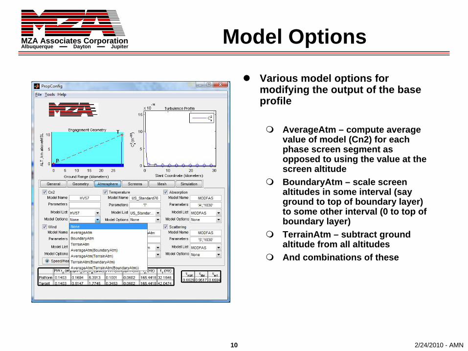
Model Options

Various model options for modifying the output of the base profile

AverageAtm – compute average value of model (Cn2) for each phase screen segment as opposed to using the value at the screen altitudeBoundaryAtm – scale screen altitudes in some interval (say ground to top of boundary layer) to some other interval (0 to top of boundary layer)TerrainAtm – subtract ground altitude from all altitudesAnd combinations of these

2/24/2010 - AMN10


Example Atmosphere

2/24/2010 - AMN11

Using all the default settings with the exception of wind speed


Phase Screen Setup

Screens tab allows the user to change the number of phase screens, how they are distributed and where they are located

Use standard settings orCustomize via the plot or the table that is displayed by clicking the “Edit Screen Info” button

Table described in later slides

Can also specify method for computing atmospheric parameters, either continuous integration of the profile or discrete based on the screen settings

By default, PropConfig loads with discrete integration

2/24/2010 - AMN12


Variation of Screen Settings

Will examine the affects of various settings for phase screen number, distribution, and location

For wave optics simulation, would like the fewest number of screens possible such that using discrete integration approximates the atmospheric parameters when continuous integration is used

Wave-optics simulations are not continuous, need to specify screensFewer screens = faster sims

For the example (from previous slide) using continuous integration would like r0 to be within 2%

Spherical r0 for Platform – between 6.72 and 7 cmSpherical r0 for Target – between 0.5025 and 0.5231 m

2/24/2010 - AMN13


Number of Screens

Experiment with different numbers of screens and placement with Equal Thickness screens

Need about 100 equally-spaced screens at mid-point of segments to get both spherical r0 values close (within 2%) to the continuous case

2/24/2010 - AMN14


Screen Distribution

Change screen distribution to Equal Strength and experiment with screen number and placement

Need at least 50 screens located at mid-points to get close to r0 values for the continuous case

2/24/2010 - AMN15


Using Model Options

2/24/2010 - AMN16

Try the model averaging option for Cn2

Go back to Atmosphere tab and select AverageAtm for Cn2 model


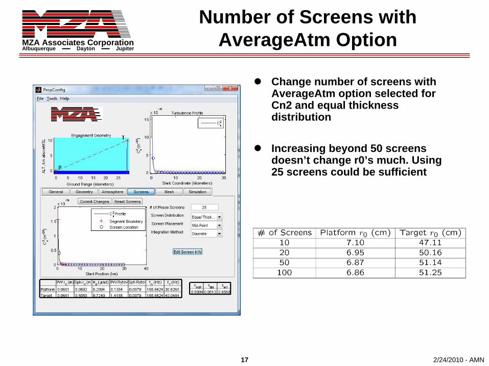
Number of Screens with AverageAtm Option

Change number of screens with AverageAtm option selected for Cn2 and equal thickness distribution

Increasing beyond 50 screens doesn’t change r0’s much. Using 25 screens could be sufficient

2/24/2010 - AMN17


Custom Screen Settings

Clicking the “Edit Screen Info” button on the Screens tab will bring up a table for viewing data in a tabular form and for customizing screen settings

In main GUI set number of screens to 10 before clicking “Edit Screen Info”Right+click to add or remove screensCan manually edit segment boundaries, screen locations, and other model data (Cn2, screen r0, Wind, Abs, etc)Can adjust screen placement and distribution to standard optionsAfter making any changes, must click “OK” or “Apply” to see how changes affect atmospheric parameters in the main windowUse “Reset” or “Cancel” to discard changes

2/24/2010 - AMN18


Example Custom Screens

Adjust screen settings and click “Apply” to see how changes affect atmospheric parametersThe above table shows one possible solution to achieve the r0’s for continuous integration using 10 screens (move first screen to 0.5 km and decrease thickness slightly)

Spherical r0 for Platform – 0.0688 m (compared to 0.0686)Spherical r0 for Target – 0.5127 m (compared to 0.5128)

2/24/2010 - AMN19


Screen Settings

Many different ways to change the settings to get similar results

May need to also monitor other atmospheric parameters

Ultimately it is up to the user to determine when the settings are “good enough” based on what the requirements are or what is needed from the simulations

2/24/2010 - AMN20


Mesh Parameters

Mesh tab contains calculations for setting propagation mesh parameters for input to a wave-optics model. Can compute parameters for either plane wave or spherical wave propagationComputes a minimum grid size and maximum pixel spacing and recommends values to be usedCan modify the turbulence blurring factor or specify minimum number of points in the aperture as needed

For the example, mesh size (propdxy) is limited by the minimum number of points in aperture

2/24/2010 - AMN21


Example Mesh

2/24/2010 - AMN22

Changing the turbulence blurring factor to 2 will yield more optimistic mesh settings (smaller grid)

From previous slide the minimum Nxy is 261, and gets rounded up to 512 (the next power of 2)


Simulation Setup

PropConfig has a built-in simulation capability based on TBWaveCalc in ATMTools.

Open-loop simulation that can include both turbulence and thermal blooming

Options includePropagation direction

Currently only propagates from an aperture

Laser typeLaser power (important for thermal blooming)Focus range of the transmitting opticsNumber of time stepsMesh can be changed independently of settings on Mesh tab.

2/24/2010 - AMN23


Example Simulation

2/24/2010 - AMN24

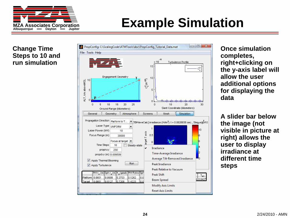
Once simulation completes, right+clicking on the y-axis label will allow the user additional options for displaying the data

A slider bar below the image (not visible in picture at right) allows the user to display irradiance at different time steps

Change Time Steps to 10 and run simulation


Other Capabilities

Output the Atm and G structures for use with other functions in ATMTools, EngagementTools, and SHaRE (via the Tools menu)

Save data to a Matlab .mat file and load data files previously saved with PropConfig (via the File menu)

Saved data file contains Atm and G structures for use with other functions in ATMTools and EngagementTools and other data necessary for populating PropConfig (wavelength, diameters, etc)

The utility keeps track of recent files/directoriesPropConfig can also load data files previously saved with TurbToolData can then be loaded into a WaveTrain runset for doing wave optics simulation or loaded into Matlab to set up an engagement in SHaRE (Scaling for High Energy Laser and Relay Engagement)

Refer to the ATMTools and EngagementTools user’s guides for more information

2/24/2010 - AMN25


Save to File

2/24/2010 - AMN26

Save the PropConfig data to a Matlab .mat file usingFile->Save…


Data in a PropConfig File

Trans_Abs 1x1 doubleTrans_Scat 1x1 doubleWavelength 1x1 doublecomputedScreenData 1x1 structmeshParamsPW 1x1 structmeshParamsSPH 1x1 structpropdxy 1x1 doublepropdxy2 1x1 doublepropnxy 1x1 doublescreens 1x1 structtargZenithProjection 1x2 doubletargZenithTP 1x2 doubletargZenithXY 1x2 double

2/24/2010 - AMN27

ATMToolsVer 1x1 structApDiamPlatform 1x1 doubleApDiamTarget 1x1 doubleAtm 1x1 structFFTbase 1x1 doubleG 1x1 structGeomSpec 1x2 charGndAlt 1x1 doubleHELFocus 1x1 doubleHELPower 1x1 doublePlatformPropMetrics 1x1 structS 1x1 structSimResults 0x0 doubleSimStatus 1x1 cellTargetPropMetrics 1x1 struct

List of variables in a PropConfig data file:


computedScreenDatacomputedScreenData =

platformAlt: 2755targetAlt: 1231

groundRange: 1.9936e+004slantRange: 2.0000e+004platformVp: 50platformVt: 0targetVp: 2.2204e-016targetVt: 0

psPositions: [20x1 double]psThicknesses: [20x1 double]

Cn2: [20x1 double]IntegratedCn2: [20x1 double]

Abs: [20x1 double]Scat: [20x1 double]Temp: [20x1 double]Lin: [20x1 double]

Lout: [20x1 double]r0Screens: [20x1 double]

wavelength4r0s: 1.3150e-006

WindVelocityP: [20x1 double]WindVelocityT: [20x1 double]EffVelocityP: [20x1 double]EffVelocityT: [20x1 double]platformVy: 50platformVx: 0targetVy: 2.2204e-016targetVx: 0

WindVelocityY: [20x1 double]WindVelocityX: [20x1 double]EffVelocityY: [20x1 double]EffVelocityX: [20x1 double]

2/24/2010 - AMN28


Pulling Data into WaveTrain

With WaveTrain 2010A, there are two options for populating a runwith data from PropConfig:1) Load the computedScreenData structure and any other parameters

needed using mliLoad. Use mliGetField to pull the required information from the data structure. Use your favorite AcsAtmSpec constructor.

This option is available in WaveTrain 2009A as well2) Call PropConfigAtmSpec, instead of AcsAtmSpec, and/or

PropConfigTBAtmSpec, instead of MtbAtmSpec, with the Matlab data file name to construct the AcsAtmSpec object

Can still use mliLoad to load any additional parameters that may be neededThe object created by PropConfigAtmSpec has methods for returning propnxy, propdxy, HEL focus range and HEL power as specified in the PropConfig data file

2/24/2010 - AMN29


PropConfigAtmSpec

Requires Matlab file name, optional inputs for turbulence multiplier, including slew wind and scaling for atmospheric transmissionThere is a constructor for AcsAtmSpec that uses an ATKAtmStruct

However, it only pulls out turbulence and screen locations/thicknessesThis new constructor can get everything needed, i.e. turbulence, wind (natural and optionally slew), inner and outer scale, wavelength and screen information

The TurbTool data file constructor for AcsAtmSpec still exists

2/24/2010 - AMN30


PropConfigTBAtmSpec

MtbAtmSpec does not have a constructor that uses ATKAtmStruct, so this new constructor simplifies things a bitAlso has the option to include slew wind

2/24/2010 - AMN31


Example System

Same old atmosphere will take:• PropConfigAtmSpec• PropConfigTBAtmSpec

2/24/2010 - AMN32


Example Runset

2/24/2010 - AMN33

PropConfigAtmSpecand PropConfigTBAtmSpecare classes derived from AcsAtmSpec and MtbAtmSpecThey can be used in any existing atmospheric path module


Applying Turbulence Factor

2/24/2010 - AMN34

Create an original AtmSpec object

Apply a turbulence factoro Makes a copy of the

original AtmSpec object with a modified turbulence strength


BLAT01

Successfully created versions of the runset BLAT01RunAtoG using data from PropConfig with v2010A-beta in mzadist

One version loads the computedScreenData structure and sets parameters and variables using mliGetField and uses AcsAtmSpec to set up the atmosphereAnother version uses PropConfigAtmSpec

Verified that results of the three runs were the sameOnce I found that the screens were being placed at beginning of segments, as opposed to mid-segment as is done in ATMTools

2/24/2010 - AMN35

PropConfig – A Tool for Atmospheric Propagation Configuration Tutorial.pdf · Data from...

Documents

Transcript of PropConfig – A Tool for Atmospheric Propagation Configuration Tutorial.pdf · Data from...