Propagating uncertainty through a non-linear hyperelastic model using advanced Monte-

Carlo methods

Paul Hauseux, Jack S. Hale and Stéphane P. A. Bordas

1

Wednesday, June 8 2016

European Congress on Computational Methods in Applied Sciences and Engineering5-10 JUNE 2016 Crete Island, Greece

Stg. No. 279578 RealTCut

2

Context Soft-tissue biomechanics simulations with uncertainty

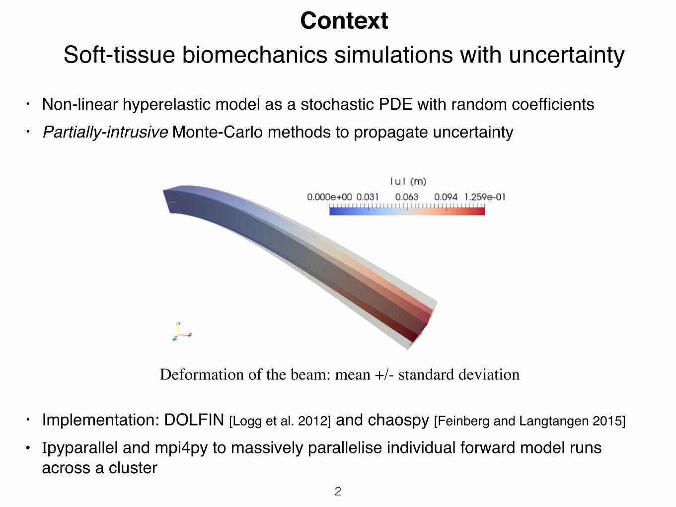
• Non-linear hyperelastic model as a stochastic PDE with random coefficients• Partially-intrusive Monte-Carlo methods to propagate uncertainty

Deformation of the beam: mean +/- standard deviation

• Implementation: DOLFIN [Logg et al. 2012] and chaospy [Feinberg and Langtangen 2015] • Ipyparallel and mpi4py to massively parallelise individual forward model runs

across a cluster

1) Monte-Carlo method

3

F (u,!) = 0

• A non-linear stochastic system:

• Expected value of a quantity of interest [Caflisch 1998]:

• The classical Monte-Carlo approach:

E( (u(x,!))) =

Z

⌦ (u(x,!)) dP (!) =

1

Z

ZX

z=1

(u(x,!z)) + o

✓|| ||p

Z

◆

E( (u(x,!)))MC ⇡ 1

Z

ZX

z=1

(u(x,!z))

(⌦,F , P )Probability space:

! = (!1,!2, . . . ,!M )Random parameters:

2) MC method with use of sensitivity information

4

E( (u(x,!)))SD�MC ⇡ 1

Z

ZX

z=1

(u(x,!z))�

MX

i=1

d

d!i(!)⇥ (!i � !i)

!

@F (u,!)

@u| {z }U⇥U

du

d!|{z}U⇥M

= � @F (u,!)

@!| {z }U⇥M

• Expected value of a quantity of interest [Cao et al. 2004]:

• Tangent linear model to evaluate the sensitivity derivatives [Farrell et al. 2013]:

U: size of the deterministic problem M: number of random parameters

u ⇡ 1

Z

ZX

z=1

u(x,!z)�

MX

i=1

du

d!i(!)⇥ (!i � !i)

!

u

2 ⇡ 1

Z

ZX

z=1

u

2(x,!z)� 2uMX

i=1

du

d!i(!)⇥ (!i � !i)

!

• First and Second moments of the displacement:

3) Multi-level MC method with use of PCE

5

• Polynomial chaos expansion (PCE) [Wiener 1936]:

• ML-MC method [Matthies 2008, Giles 2015]:

u

k(x,!) =X

↵2JM,p

u

k↵(x)H↵(!)

dim(JM,p) = (M + p)!/(M !p!)

4) 3D Numerical simulations

6

• The stored strain energy density function for a compressible Mooney–Rivlin material:

W = C1(I1 � 3) + C2(I2 � 3) +D1(detF� 1)2

120000 d.o.f

⇢(!1) = ⇢0(1 + !1/2)

⇧ = Wdx� ⇢gdx,�g = g~y, g = 9.81 m.s�2

�• The total potential energy:

• 2 RV with beta(2,2) distribution:D1(!2) = D0

1(1 + !2)

8>><

>>:

D01 = 2 · 105 Pa

C2 = 2 · 105 PaC1 = 104 Pa⇢0 = 600 kg/m3

Fig: Mesh, initial configuration and deformed configuration.

4) 3D Numerical simulations

7

10 100 1000 10000 1e+05Z

-0.13

-0.125

-0.12

-0.115

-0.11

u ymax

(m)

MCMC-SDML-MC

Mean

4) 3D Numerical simulations

8

10 100 1000 10000 1e+05Z

0

0.005

0.01

0.015

0.02

u ymax

(m)

MCMC-SDML-MC

Std

4) 3D Numerical simulations

9

Mean: influence of the number of levels

1000 10000Z

-0.125

-0.12

-0.115

u ymax

(m)

MCN = 2N = 3N = 4N = 6

4) 3D Numerical simulations

10

Global and local sensitivity analysis [Sobol 2001, Sudret 2008]

!2 !1��� dud!

i

��� 1.64 4.36

|dumax

y

d!i

| 0.014 0.036

|dumax

x

d!i

| 0.0081 0.021

umax

x

umax

y

!2 !1 !2 !1

First order 0.136 0.862 0.133 0.867Total e↵ect 0.138 0.862 0.133 0.868

Table 1: Local sensitivity around mean parameters

Table 2: Sobol’s sensitivity indices (global sensitivity) for the quantities of interest

4) 3D Numerical simulations

11

|umax

y

|(mm) MC-simulations (Z=18000)

Computational time with 120 engines running in parallel: comparison between the different methods with a number of realisations to have an accurate solution

(MC with Z = 18000, MC-SD with Z = 1000 and ML-MC with Z = 4500).

MC MC-SD ML-MCT (min) 1100 65 225

Conclusion

12

• By using sensitivity information and multi-level methods with polynomial chaos expansion we demonstrate that computational workload can be reduced by one order of magnitude over commonly used schemes

• Implementation: DOLFIN [Logg et al. 2012] and chaospy [Feinberg and Langtangen 2015]

• Ipyparallel and mpi4py to massively parallelise individual forward model runs across a cluster

• Partially-intrusive Monte-Carlo methods to propagate uncertainty