Proofs of randomized algorithms in Coq

Philippe Audebaud

LIP - ENS Lyon46, allee d’Italie - 69437 Lyon - France

Christine Paulin-Mohring

INRIA Futurs, ProVal - Parc Orsay Universite - F-91893LRI, Univ Paris-Sud, CNRS - Orsay F-91405

Abstract

Randomized algorithms are widely used for finding efficiently approximated solu-tions to complex problems, for instance primality testing and for obtaining goodaverage behavior. Proving properties of such algorithms requires subtle reasoningboth on algorithmic and probabilistic aspects of programs. Thus, providing toolsfor the mechanization of reasoning is an important issue. This paper presents a newmethod for proving properties of randomized algorithms in a proof assistant basedon higher-order logic. It is based on the monadic interpretation of randomized pro-grams as probabilistic distributions (Giry, 1982; Ramsey and Pfeffer, 2002). It doesnot require the definition of an operational semantics for the language nor the de-velopment of a complex formalization of measure theory. Instead it uses functionaland algebraic properties of unit interval. Using this model, we show the validity ofgeneral rules for estimating the probability for a randomized algorithm to satisfyspecified properties. This approach addresses only discrete distributions and givesrules for analysing general recursive functions.

We apply this theory to the formal proof of a program implementing a Bernoullidistribution from a coin flip and to the (partial) termination of several programs.All the theories and results presented in this paper have been fully formalized andproved in the Coq proof assistant.

Key words: randomized algorithms, proof of partial and total correctness,functional language, axiomatic semantics, probability framing, call-by-value,monadic interpretation

Email addresses: Philippe.Audebaud@ens-lyon.fr (Philippe Audebaud),Christine.Paulin@lri.fr (Christine Paulin-Mohring).

Article published in Science of Computer Programming 74 (2009) 568–589

1 Introduction

Randomized algorithms are widely used either for finding efficient approximatesolutions to complex problems such as primality testing, or in order to obtaingood average behavior. Proving properties of such algorithms requires subtlereasoning about both algorithmic and probabilistic aspects of programs. Pro-viding tools for the mechanization of reasoning is consequently an importantissue.

1.1 Models

The first problem is to find an appropriate mathematical representation of arandomized algorithm. Methods for modeling randomized programs go backto the early work of Kozen (1981, 1983) which proposes to interpret random-ized imperative programs as measure transformers. This approach has beenstudied further by Morgan and McIver (1999) who extend the interpretationto non-deterministic as well as probabilistic choices and define a refinementrelation. Using an extension of weakest-precondition computation to random-ized programs, they propose a method to lower the probability for the resultof the program to satisfy a given property.

Studying the semantic foundations of probabilistic languages has been theconcern of much research. There are at least two different approaches.

The first one is an operational view using access to an arbitrary number ofindependent random variables following a given distribution: which can be acoin flip (Hurd, 2002b, 2003) or a uniform distribution (Park et al., 2005). Thisinterpretation is a monadic transformation. If Ω denotes the type of infinitesequences of independent random values, then a computation of type A willbe interpreted as a function of type Ω → A× Ω: it computes a value of typeA and modifies the global state of type Ω after consuming a finite prefix ofthe sequence of random values. Reasoning on randomized programs using thisapproach requires to model the base probability distribution on Ω.

The second approach uses an interpretation of randomized programs as prob-ability distributions. It is also possible to use a syntactic monadic transforma-tion. In the discrete case, a probability distribution can be represented as afunctional mapping from a subset of some σ into the interval [0, 1], or, usingexpectation, mapping a real-valued function on σ into an element of R. Themonadic structure of probability theory was studied in Giry (1982) develop-ing unpublished ideas in Lawvere (1962). This approach is used for instance inRamsey and Pfeffer (2002) where a randomized functional term is interpretedas an Haskell program using the so-called expectation monad, ie functions of

569

type (σ → R)→ R.

1.2 Proofs

Enabling the mechanized reasoning of probabilistic programs requires alsotools for analysing the behavior of these programs. This point is a researchtopic.

Hurd, McIver and Morgan designed a mechanization of the quantitative logicfor probabilistic guarded commands using the proof assistant HOL (Hurdet al., 2005). Their goal is very similar to ours, except that they analyse adifferent source language, handling both probabilistic and non-deterministicchoice in an imperative settings, while we are only considering probabilisticchoice but in a functional language, including recursive functions. Their workalso contains the formalisation in HOL of meta-reasoning on the source lan-guage, while we have for the moment only considered a shallow embedding ofour programs in Coq.

With regard to algorithms, Hurd (2002b, 2003) shows how to model andprove properties of randomized programs in the HOL proof assistant using amonadic transformation of programs, where Hurd assumes access to an infinitesequence of independent coin flips.

1.3 Our choices

In this article, we intend to prove specifications for probabilistic programs in-side the Coq proof assistant. We start by turning a (probabilistic) functionalprogram p on some type A into a pure functional term, denoted as [p], withtype MA ≡ (A→ [0, 1])→ [0, 1], where MA is provided with a monadic struc-ture. In this setting, [p] will represent a (mathematical) discrete measure: asub-probability. Although this monad appears more restrictive than the oneproposed in Ramsey and Pfeffer (2002), it turns out to be sufficient for thegoal of providing approximations for probabilities. To keep the monadic trans-formation simple, we design a tiny probabilistic language Rml, equipped witha rather restricted type system, yet expressive enough for coding interestingalgorithms. Program specifications are then proved along a specific inferencesystem for axiomatic semantics.

For the proof assistant, tools are required for interactive reasoning about prob-abilistic programs (actually through the above transformation). We thus shareHurd’s approach, while our design choices do not require full development ofmeasure theory inside Coq. Our tools are based upon a specific library which

570

axiomatizes the properties required on some abstract type U representingthe real interval [0, 1]. This library is developed as an independent contri-bution (Paulin-Mohring, 2007), and designed to provide the back-end toolsneeded by the user.

Our axiomatic semantics enhances previous work by Morgan and McIver(1999), where rules allowed only weakening for probabilities. We prove theirvalidity with respect to our semantics. We also propose schemes to reason ongeneral recursive functions which generalize the usual schemes for loops.

Our framework does not rely on a particular choice of a primitive randomizedfunction. In this paper, we use a boolean flip and a finite random functionand we show how to interpret directly a randomized choice operator. We onlybuild discrete distributions: dealing with continuous distributions would re-quire modification of the interpretation to restrict the functional to measurablefunctions, an extension we plan to investigate later.

1.4 Paper outline

The paper is organized as follows. In Section 2, we introduce the input lan-guage and its semantics: an interpretation of programs as measures usinga monadic transformation. We analyze our monadic interpretation from thefunctional point of view. In Section 3 we introduce the basic Coq theories forrepresenting measures. In Section 4, we show the derived rules for framing theprobability for a randomized program to satisfy a given property, in particularfor the case of recursive programs. In Section 5, we apply our method to proofsof simple probabilistic properties of programs.

The current paper extends Audebaud and Paulin-Mohring (2006) by suggest-ing an interpretation of higher-order functional programs in section 2.5.6 andintroducing rules for intervals in section 4.1 and also more general rules forreasoning on recursive functions in section 4.4. We also develop an example ofpartial termination in section 5.2.

1.5 Remark

The possible interpretation of random functional programs as probabilisticdistributions using a monadic interpretation is not new, it appears in manytheoretical works on semantics, see Giry (1982), or more concretely for rep-resenting random programs in Haskell by Ramsey and Pfeffer (2002). To ourknowledge, however, the approach of mechanizing reasoning about randomfunctional expressions is new. In Ramsey and Pfeffer (2002), the interpreta-

571

tion does not cover general recursive programs and its inefficiency is criticized,the authors propose instead an alternative method which only covers discretedistributions. The possibility to cover recursion was however studied in Jones(1989), on which the approach of this paper is based. That the interpreta-tion can lead to inefficient or even unfeasible computations in practice will beillustrated in Sections 2.6.1 and 2.6.2. Our work advocates that operationalbehavior is not relevant, since our model allows anyway for abstract reasoningon programs, using the general rules presented in Section 4 and illustratedon examples in Section 5. This is to be related to Hoare rules for axiomaticsemantics, which do not rely on computations per se, but to denotational se-mantics. From this point of view, we compare with Kozen’s second semanticsin Kozen (1981), and to the framework proposed in (Kozen, 1983).

2 Monadic interpretation of randomized algorithms

Sections 2.1 and 2.2 provide background results on probabilities which underlieour framework. We present in Section 2.3 a reasonably simple probabilisticlanguage Rml. The monadic interpretation is the subject of Section 2.4, wherewe discuss also the consequences of relaxing the typing rules. We concludethis section by putting our interpretation at work on concrete examples inSection 2.6.

The approach in this part is very similar to the one proposed in Ramsey andPfeffer (2002). The main differences are that we measure functions with valuesin the interval [0, 1] instead of real numbers, we concentrate on a first-orderlanguage, which is sufficient for the applications we want to address, but wealso show how to extend the approach for the general functional case. Unlikewhat is done in Ramsey and Pfeffer (2002), we shall address the question ofgeneral recursive functions in section 4.

2.1 Randomized programs as measure transformers

Usually, an imperative or functional program returns at most one state (orvalue in the functional case), from any given initial state. Moreover, the re-turned state is entirely determined by the program and the initial state. Whendealing with probabilistic programs, this is no longer the case, even when run-ning the program several times, starting with the same initial state. Rather,the distribution of returned states can be represented as some random vari-able, hence a measure over the states set. This change of view has been investi-gated in works by Kozen (1981, 1983); Jones and Plotkin (1989); Jones (1989);McIver and Morgan (2005) among others. Whilst the observation of the actual

572

returned states is non-deterministic, the measure which can be built from theinitial state by applying the denotation of a probabilistic program providesa deterministic value. This approach is then easily extended into randomizedprograms viewed as measure transformers.

The distribution of these output states is interesting. If this distribution isknown, given a property P on the output state, we can compute the probabil-ity for the result of the program to satisfy P . A randomized program uses basicrandomized primitives such as a random function which, given a natural num-ber n, produces a number between 0 and n with uniform probability 1

1+n, or a

more basic flip function which produces boolean values true or false withequal probability 1

2. Another classical operator is probabilistic choice P p+ Q

which behaves like the program P with probability p and as Q with probability1−p.

The implicit assumption is that any access to a given random primitive in theprogram is independent of the others.

Since we are concerned with a functional language, we do not have to takeglobal states into consideration. Programs are interpreted as functions whichcompute values, and our aim is to estimate the distribution of these returnvalues.

2.2 Representation of distributions

In this section, we explain our choice for a mathematical representation ofprobability distributions. We introduce the notation [0, 1] for the set of realnumbers x such that 0 ≤ x ≤ 1.

2.2.1 The measure perspective

A (positive) measure on a set A, is a linear functional µ which given a (mea-surable) function f from A to R+, computes a non-negative real number, itsintegral

∫fdµ. A required condition on µ to be a measure, besides linearity,

is that µ preserves least upper bounds :∫ ∨

n fndµ =∨n

∫fndµ.

In the following, we shall use the notation µ(f) instead of∫fdµ.

2.2.2 Notations for characteristic functions

If X is a subset of A, IX ∈ A → [0, 1] will denote the characteristic functionof X such that ∀x ∈ A, IX(x) = 0⇔ x 6∈ X ∧ IX(x) = 1⇔ x ∈ X. We write

573

simply I for the function which is 1 everywhere. If P (x) is a formula with afree variable x, we write IP (.) for the characteristic function of the set X suchthat x ∈ X ⇔ P (x). For instance, I.=k is the characteristic function of thesingleton k.

2.2.3 Our abstract notion of measure

From now on in this article, probability distributions are represented as posi-tive measures, which norm is bounded by 1.

In order to define a probability distribution, it is sufficient to be able to mea-sure functions which take values in the unit interval [0, 1]. We can remarkthat if ∀x.f(x) ∈ [0, 1] then µ(f) ∈ [0, 1] because a probability distribution isbounded by one. Hence, a measure µ on A can be interpreted as a functionof type (A → [0, 1]) → [0, 1] satisfying some extra algebraic properties, to beprecised in section 3.2.

2.3 Basic language for randomized programs

For sake of simplicity, we shall use in the following a simple first-order func-tional language. We will explain in section 2.5.6 how it could be extended tofull functional constructions.

2.3.1 Expressions

Our language (called Rml) contains the following constructions:

• Variables: x• Primitive constants: c• Conditional: if b then e1 else e2• Local binding: let x = e1 in e2• Application: f e1 . . . en with f a primitive or user-defined function.

We shall introduce parentheses in concrete notations when needed.

Functions can be declared the following way:

let f x1 . . . xn = e

Remark. Recursive definitions can be defined as well:

let rec f x1 . . . xn = e

574

However, their introduction raise some technical issues with respect to thematerial developed in this section. Therefore, we postpone any further detailto section 3.3.

In order to deal with probabilistic programs, Rml includes also a few randomprimitive functions, such as the random function which given a positive integern, computes with uniform distribution an integer k such that 0 ≤ k ≤ n andthe flip function which computes a boolean which is true with probability 1

2.

2.3.2 Types

Our assumption on Rml, is that all expressions will be well-formed using arestricted simple types system. This system is built over base types such asbool for boolean values and nat for natural numbers (non-negative integers),and allows arrow types in the restricted case where arguments have a base type.In the following we write β, βi . . . in order to denote a base type. We shall writee : β when e is a well-formed expression of type β and f : β1 → · · · → βn → βwhen f e1 . . . en : β whenever ei : βi for i = 1 . . . n.

2.3.3 Meta-language

Randomized expressions are interpreted in an higher-order functional lan-guage. The target type system is richer: a type τ will be either a base type β(including the base type [0, 1] for reals between 0 and 1) or some functionaltype τ1 → τ2.

We use the same notations as in Rml for local bindings and conditionals, butwe also introduce typed abstraction fun (x : τ) ⇒ e and binary application(e1 e2). Application is left associative and types can be omitted in lambda-abstraction, written fun x ⇒ e, when the type is clear from the context.As a matter of fact, Rml (except for the randomized primitive functions)corresponds to a restricted subset of our meta-language where variables arealways in base types and functions are in eta-long normal form.

An alternative could have been to use a monadic meta-language as in Moggi(1991) or Pfenning and Davies (2001), but it would have introduced an extralevel of syntax that we are able to avoid here, owing to the restrictions on Rmlsyntax. Doing otherwise would result in introducing more complex notations,which would have obscure the key ideas. The section 2.5.6 develops thesepoints further.

575

2.4 Interpretation of random expressions

A (random) expression e in a base type β actually represents a set of values oftype β, as different evaluations of the expression will lead to different valuesin general.

As pointed out above, for analyzing the distribution of these values, we inter-pret e : β as a measure on β, i.e. a function of type (β → [0, 1]) → [0, 1]. Inthe following, Mτ will represent the type (τ → [0, 1]) → [0, 1] of measures onvalues of type τ .

We write [e] to represent the measure associated to the expression e. If weknow [e], given a property Q on β, it is possible to compute the probabilityfor the evaluation of e to satisfy Q, it is just [e]IQ, namely the application ofthe measure associated to the expression e to the characteristic function ofthe predicate Q, interpreted as a subset of β.

2.5 Monadic transformation

The interpretation of e of type β as a measure [e] of type Mβ = (β → [0, 1])→[0, 1] is defined by structural induction on e.

2.5.1 Definition of unit and bind

As usual in monadic transformations, we first introduce two operators:

unit : τ → Mτ

= fun (x : τ)⇒ fun (f : τ → [0, 1])⇒ f x

bind : Mτ → (τ → Mσ)→ Mσ

= fun (µ : Mτ)⇒ fun (M : τ → Mσ)⇒

fun (f : σ → [0, 1])⇒ µ (fun (x : τ)⇒M x f)

As expected, theses definitions satisfy the usual monadic properties. Theequality on Mβ is defined point-wise (µ1 = µ2 ⇔ ∀f, µ1(f) = µ2(f)).

• bind (unit x) M = M x• bind (bind µ M1) M2 = bind µ (fun x⇒ bind (M1 x) M2)• bind µ unit = µ

576

2.5.2 Interpretation of functions

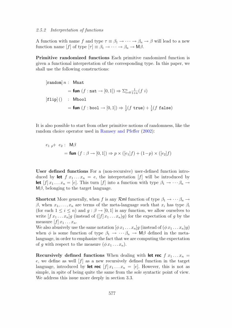
A function with name f and type τ ≡ β1 → · · · → βn → β will lead to a newfunction name [f ] of type [τ ] ≡ β1 → · · · → βn → Mβ.

Primitive randomized functions Each primitive randomized function isgiven a functional interpretation of the corresponding type. In this paper, weshall use the following constructions:

[random]n : Mnat

= fun (f : nat→ [0, 1])⇒ Σni=0

11+n

(f i)

[flip] () : Mbool

= fun (f : bool→ [0, 1])⇒ 12(f true) + 1

2(f false)

It is also possible to start from other primitive notions of randomness, like therandom choice operator used in Ramsey and Pfeffer (2002):

e1 p+ e2 : Mβ

= fun (f : β → [0, 1])⇒ p× ([e1]f) + (1−p)× ([e2]f)

User defined functions For a (non-recursive) user-defined function intro-duced by let f x1 . . . xn = e, the interpretation [f ] will be introduced bylet [f ]x1 . . . xn = [e]. This turn [f ] into a function with type β1 → · · · βn →Mβ, belonging to the target language.

Shortcut More generally, when f is any Rml function of type β1 → · · · βn →β, when x1, . . . , xn are terms of the meta-language such that xi has type βi(for each 1 ≤ i ≤ n) and g : β → [0, 1] is any function, we allow ourselves towrite [f x1 . . . xn]g (instead of ([f ]x1 . . . xn)g) for the expectation of g by themeasure [f ]x1 . . . xn.We also abusively use the same notation [φx1 . . . xn]g (instead of (φx1 . . . xn)g)when φ is some function of type β1 → · · · βn → Mβ defined in the meta-language, in order to emphasize the fact that we are computing the expectationof g with respect to the measure (φx1 . . . xn).

Recursively defined functions When dealing with let rec f x1 . . . xn =e, we define as well [f ] as a new recursively defined function in the targetlanguage, introduced by let rec [f ]x1 . . . xn = [e]. However, this is not assimple, in spite of being quite the same from the sole syntactic point of view.We address this issue more deeply in section 3.3.

577

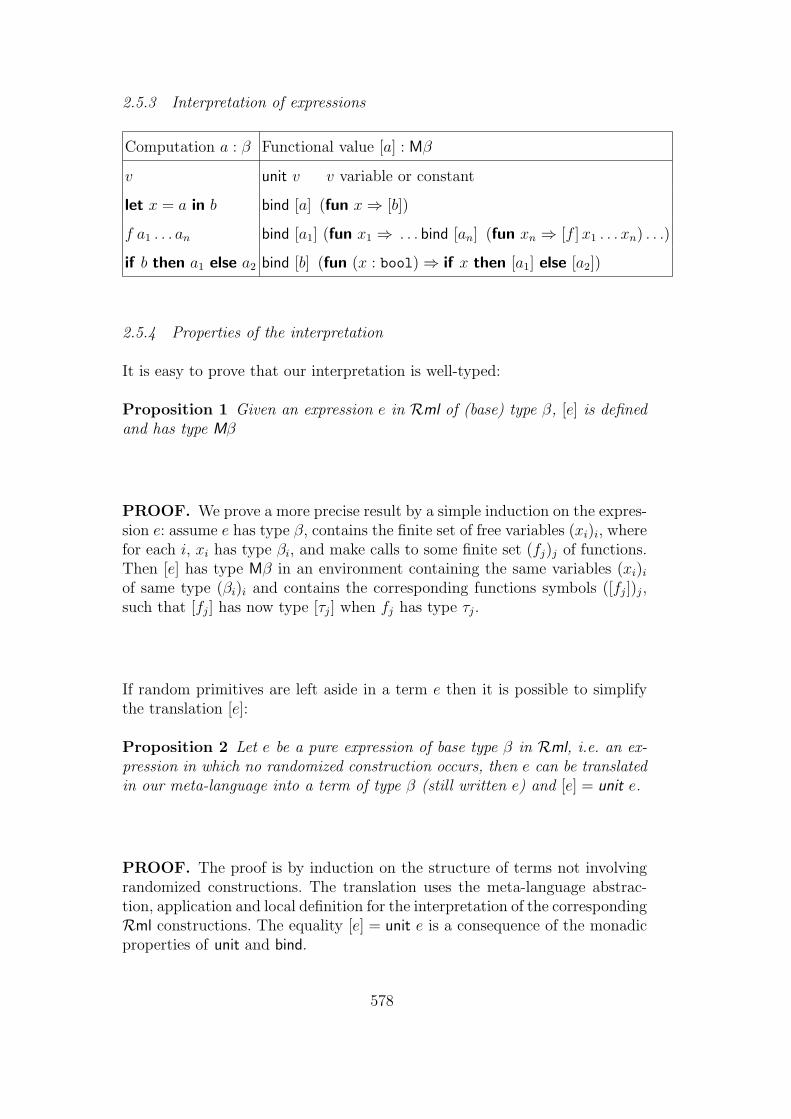
2.5.3 Interpretation of expressions

Computation a : β Functional value [a] : Mβ

v unit v v variable or constant

let x = a in b bind [a] (fun x⇒ [b])

f a1 . . . an bind [a1] (fun x1 ⇒ . . . bind [an] (fun xn ⇒ [f ]x1 . . . xn) . . .)

if b then a1 else a2 bind [b] (fun (x : bool)⇒ if x then [a1] else [a2])

2.5.4 Properties of the interpretation

It is easy to prove that our interpretation is well-typed:

Proposition 1 Given an expression e in Rml of (base) type β, [e] is definedand has type Mβ

PROOF. We prove a more precise result by a simple induction on the expres-sion e: assume e has type β, contains the finite set of free variables (xi)i, wherefor each i, xi has type βi, and make calls to some finite set (fj)j of functions.Then [e] has type Mβ in an environment containing the same variables (xi)iof same type (βi)i and contains the corresponding functions symbols ([fj])j,such that [fj] has now type [τj] when fj has type τj.

If random primitives are left aside in a term e then it is possible to simplifythe translation [e]:

Proposition 2 Let e be a pure expression of base type β in Rml, i.e. an ex-pression in which no randomized construction occurs, then e can be translatedin our meta-language into a term of type β (still written e) and [e] = unit e.

PROOF. The proof is by induction on the structure of terms not involvingrandomized constructions. The translation uses the meta-language abstrac-tion, application and local definition for the interpretation of the correspondingRml constructions. The equality [e] = unit e is a consequence of the monadicproperties of unit and bind.

578

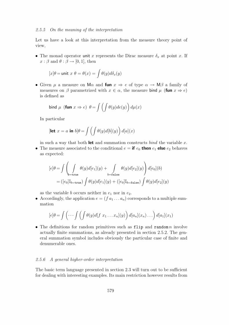
2.5.5 On the meaning of the interpretation

Let us have a look at this interpretation from the measure theory point ofview,

• The monad operator unit x represents the Dirac measure δx at point x. Ifx : β and θ : β → [0, 1], then

[x]θ= unit x θ = θ(x) =∫θ(y)dδx(y)

• Given µ a measure on Mα and fun x ⇒ e of type α → Mβ a family ofmeasures on β parametrized with x ∈ α, the measure bind µ (fun x⇒ e)is defined as

bind µ (fun x⇒ e) θ=∫ (∫

θ(y)de(y))dµ(x)

In particular

[let x = a in b]θ=∫ (∫

θ(y)d[b](y))d[a](x)

in such a way that both let and summation constructs bind the variable x.• The measure associated to the conditional e = if e0 then e1 else e2 behaves

as expected:

[e]θ=∫ ∫

b=true

θ(y)d[e1](y) +∫

b=false

θ(y)d[e2](y)

d[e0](b)

= ([e0]Ib=true)∫θ(y)d[e1](y) + ([e0]Ib=false)

∫θ(y)d[e2](y)

as the variable b occurs neither in e1 nor in e2.• Accordingly, the application e = (f a1 . . . an) corresponds to a multiple sum-

mation

[e]θ=∫ (· · ·

∫ (∫θ(y)d[f x1 . . . xn](y)

)d[an](xn) . . .

)d[a1](x1)

• The definitions for random primitives such as flip and randomn involveactually finite summations, as already presented in section 2.5.2. The gen-eral summation symbol includes obviously the particular case of finite anddenumerable ones.

2.5.6 A general higher-order interpretation

The basic term language presented in section 2.3 will turn out to be sufficientfor dealing with interesting examples. Its main restriction however results from

579

its proper design: we do not take into account programs which could generaterandomized functions. For instance, the program Φ defined as

let Φ = let x = random 100 in fun (n:nat) ⇒ let y = random n in y+x

provides a random variable on type nat→ nat. As such, one would expect itsmonadic interpretation to be given over some type expression [[nat→ nat]] ≡Mρ ≡ (ρ → [0, 1]) → [0, 1], where ρ is some type, which is described moreprecisely below.

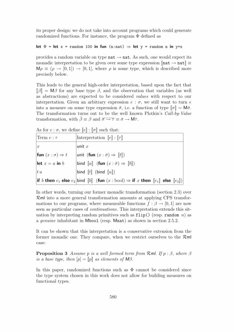
This leads to the general high-order interpretation, based upon the fact that[[β]] = Mβ for any base type β, and the observation that variables (as wellas abstractions) are expected to be considered values with respect to ourinterpretation. Given an arbitrary expression e : σ, we still want to turn einto a measure on some type expression σ, i.e. a function of type [[σ]] = Mσ.The transformation turns out to be the well known Plotkin’s Call-by-Valuetransformation, with β ≡ β and σ → τ ≡ σ → Mτ .

As for e : σ, we define [[e]] : [[σ]] such that:

Term e : τ Interpretation [[e]] : [[τ ]]

x unit x

fun (x : σ)⇒ t unit (fun (x : σ)⇒ [[t]])

let x = a in b bind [[a]] (fun (x : σ)⇒ [[b]])

t u bind [[t]] (bind [[u]])

if b then e1 else e2 bind [[b]] (fun (x : bool)⇒ if x then [[e1]] else [[e2]])

In other words, turning our former monadic transformation (section 2.3) overRml into a more general transformation amounts at applying CPS transfor-mations to our programs, where measurable functions f : β → [0, 1] are nowseen as particular cases of continuations . This interpretation extends this sit-uation by interpreting random primitives such as flip() (resp. random n) asa genuine inhabitant in Mbool (resp. Mnat) as shown in section 2.5.2.

It can be shown that this interpretation is a conservative extension from theformer monadic one. They compare, when we restrict ourselves to the Rmlcase:

Proposition 3 Assume p is a well formed term from Rml. If p : β, where βis a base type, then [p] = [[p]] as elements of Mβ.

In this paper, randomized functions such as Φ cannot be considered sincethe type system chosen in this work does not allow for building measures onfunctional types.

580

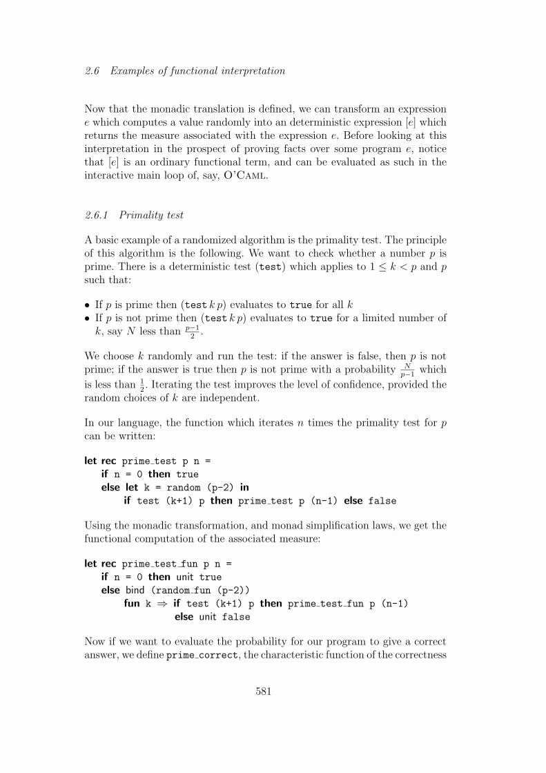
2.6 Examples of functional interpretation

Now that the monadic translation is defined, we can transform an expressione which computes a value randomly into an deterministic expression [e] whichreturns the measure associated with the expression e. Before looking at thisinterpretation in the prospect of proving facts over some program e, noticethat [e] is an ordinary functional term, and can be evaluated as such in theinteractive main loop of, say, O’Caml.

2.6.1 Primality test

A basic example of a randomized algorithm is the primality test. The principleof this algorithm is the following. We want to check whether a number p isprime. There is a deterministic test (test) which applies to 1 ≤ k < p and psuch that:

• If p is prime then (test k p) evaluates to true for all k• If p is not prime then (test k p) evaluates to true for a limited number ofk, say N less than p−1

2.

We choose k randomly and run the test: if the answer is false, then p is notprime; if the answer is true then p is not prime with a probability N

p−1which

is less than 12. Iterating the test improves the level of confidence, provided the

random choices of k are independent.

In our language, the function which iterates n times the primality test for pcan be written:

let rec prime test p n =

if n = 0 then true

else let k = random (p-2) inif test (k+1) p then prime test p (n-1) else false

Using the monadic transformation, and monad simplification laws, we get thefunctional computation of the associated measure:

let rec prime test fun p n =

if n = 0 then unit true

else bind (random fun (p-2))

fun k ⇒ if test (k+1) p then prime test fun p (n-1)

else unit false

Now if we want to evaluate the probability for our program to give a correctanswer, we define prime correct, the characteristic function of the correctness

581

predicate, which says that the result is true exactly when p is prime:

let prime correct p b = if b = exact prime p then 1. else 0.

One can now explicitly compute the probability that our program gives acorrect answer after n iterations:

let evaluate p n = prime test fun p n (prime correct p)

The function can be run in O’Caml and gives the following results.

# evaluate 23 1;;

- : float = 1

# [evaluate 9 0;evaluate 9 1;evaluate 9 2;evaluate 9 3];;

- : float list = [0.;0.75;0.9375;0.984375]

If the number is prime (example p = 23), then the result will be correct withprobability one. On the other hand, if p is not prime (example p = 9) thenthe probability that the program gives a correct answer after 0 iteration is 0,after 1 iteration, we get the good answer 3 times out of 4 and it goes to morethan 98% of good answers after 4 iterations.

One nice point is that we have been able to compute these probabilities with asimple ML program without any specific knowledge on probability theory nornumber theory (except for the interpretation of random). On the other hand,if we analyze the program, we remark that it is very inefficient:

• in order to build the characteristic function to be tested we need to know(or to test) exactly if p is prime or not;• because of the interpretation of random, the program is executed for all the

values of k between 1 and p − 1 before computing the average number ofgood answers.

2.6.2 Random walk

Furthermore, this computational approach does not work in all cases. Ourprevious program uses a structural recursion which always terminates. Manyinteresting probabilistic programs only terminate with probability one, whichis a weaker requirement. For instance the following function flips a coin andreturns how many flips it took to get false, this is a typical example of arandom walk:

let rec walk x = if flip () then x else walk (x+1)

582

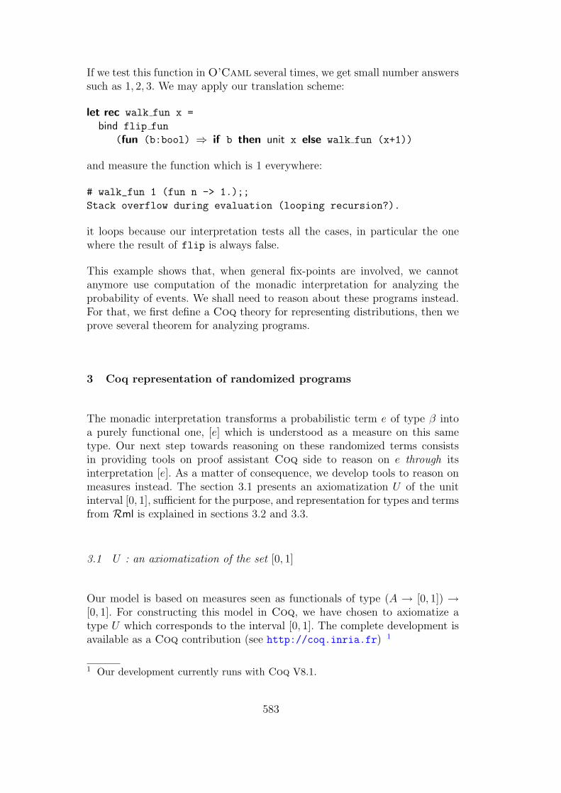
If we test this function in O’Caml several times, we get small number answerssuch as 1, 2, 3. We may apply our translation scheme:

let rec walk fun x =

bind flip fun

(fun (b:bool) ⇒ if b then unit x else walk fun (x+1))

and measure the function which is 1 everywhere:

# walk_fun 1 (fun n -> 1.);;

Stack overflow during evaluation (looping recursion?).

it loops because our interpretation tests all the cases, in particular the onewhere the result of flip is always false.

This example shows that, when general fix-points are involved, we cannotanymore use computation of the monadic interpretation for analyzing theprobability of events. We shall need to reason about these programs instead.For that, we first define a Coq theory for representing distributions, then weprove several theorem for analyzing programs.

3 Coq representation of randomized programs

The monadic interpretation transforms a probabilistic term e of type β intoa purely functional one, [e] which is understood as a measure on this sametype. Our next step towards reasoning on these randomized terms consistsin providing tools on proof assistant Coq side to reason on e through itsinterpretation [e]. As a matter of consequence, we develop tools to reason onmeasures instead. The section 3.1 presents an axiomatization U of the unitinterval [0, 1], sufficient for the purpose, and representation for types and termsfrom Rml is explained in sections 3.2 and 3.3.

3.1 U : an axiomatization of the set [0, 1]

Our model is based on measures seen as functionals of type (A → [0, 1]) →[0, 1]. For constructing this model in Coq, we have chosen to axiomatize atype U which corresponds to the interval [0, 1]. The complete development isavailable as a Coq contribution (see http://coq.inria.fr) 1

1 Our development currently runs with Coq V8.1.

583

3.1.1 Notations for complete partial orders

Our development extensively uses the notion of complete partial order. OurCoq library consequently starts with the definition of a structure for orderedsets, and one for complete partial orders.

An ordered set is given by a type O, a relation ≤ which is reflexive andtransitive. An equality on O is defined by x == y iff x ≤ y ∧ y ≤ x. Giventwo ordered sets O1 and O2, we introduce the type of monotonic functionsO1

m→ O2.

A ω-complete partial order (ω-cpo) is given by an ordered set D, a minimalelement 0 and a least-upper bound operation lub f on monotonic sequencesf : nat

m→ D. Given two ω-cposD1 andD2, a monotonic function F : D1m→ D2

is defined to be continuous whenever F (lub f) ≤ lub(F f). Because theopposite inequality is always provable, a continuous function also satisfiesF (lub f) == lub(F f).

There is a standard way to introduce fix-points in an ω-cpo D. Let F be amonotonic operator on D (ie F : D

m→ D), we introduce the sequence Fndefined by Fn ≡ F n0 (with F n+1 = F F n) and define fix F = lubFn.

It is easy to show that fix F ≤ F (fix F ), the equality fix F == F (fix F )requires that F is continuous.

The ω-cpo structure can be extended to functions spaces. If we have an ω-cpostructure on a set D, then we can define the same structure on the set A→ Dof functions with values in D, just taking:

f ≤A→D g ⇔ ∀x, f x ≤D g x

0A→D = fun x⇒ 0D lubA→Dfn = fun x⇒ lubD(fn x)

Given an ordered set O and an ω-cpo D, the set of monotonic functions fromO to D is also an ω-cpo.

3.1.2 Definitions

Our axiomatisation of [0, 1], starts by introducing an ω-cpo U . Consequentelywe can use the following symbols:

• Constant : 0• Predicates : x ≤ y, x == y with x, y ∈ U• Least-upper bounds for monotonic sequences: lub f with f ∈ nat

m→ U .If f is an expression with a free variable n, we write lub(f)n instead of

584

lub (fun n⇒ f).

We also introduce the following constructions building new elements in U :

• bounded addition: x+ y with x, y ∈ U• multiplication: x× y with x, y ∈ U• inverse: 1−x with x ∈ U• values: 1

1+nwith n : nat

The addition in U is bounded: it gives the minimum of addition on reals and 1.

3.1.3 Axioms

In addition to the ω-cpo properties, we introduce a set of axioms for theoperations on U .

3.1.3.1 Order We assume that 1 is different from 0 and not less than anyelement in U and that the order is total:

• Non-confusion: ¬0 == 1• Bounds: ∀x, x ≤ 1• Totality: ∀xy, x ≤ y ∨c y ≤ x

Coq implements an intuitionistic logic, we did not want to commit ourselves toa classical axiomatisation of real numbers. Consequentely, we choose a classicalversion of disjunction for expressing the totality: the property A∨cB is definedas ∀C, (¬¬C → C) → (A → C) → (B → C) → C and we added an axiomstating that the order relation is classical:

• Classical: ¬¬(x ≤ y)→ x ≤ y

3.1.3.2 Addition, multiplication and inverse As expected, we includethe usual axioms stating that addition and multiplication are symmetric andassociative, with 0 and 1 as their respective neutral elements.

Some properties of addition are only valid when there is no overflow duringaddition. The non-overflow condition is expressed in our formalism as x ≤ 1−y.

We express the relationship between least upper bounds (lubs) and additionand multiplication by the assumption of continuity of addition and multipli-cation with respect to their second argument.

585

The complete set of axioms is:

• Addition· Symmetry: ∀x y, x+ y == y + x· Associativity: ∀x y z, x+ (y + z) == (x+ y) + z· Neutral element: ∀x, 0 + x == x· Compatibility: ∀x y z, y ≤ z ⇒ x+ y ≤ x+ z· Simplification: ∀x y z, z ≤ 1− x⇒ x+ z ≤ y + z ⇒ x ≤ y· lub and addition: ∀(f : nat

m→ U) k, k + lub f ≤ lub(k + f n)n• Multiplication· Symmetry: ∀x y, x× y == y × x· Associativity: ∀x y z, x× (y × z) == (x× y)× z· Neutral element: ∀x, 1× x == x· Distributivity on addition: ∀x y z, x ≤ 1−y ⇒ (x+y)×z == x×z+y×z· Compatibility: ∀x y z, y ≤ z ⇒ x× y ≤ x× z· Simplification: ∀x y z,¬0 == z ⇒ z × x ≤ z × y ⇒ x ≤ y· lub and multiplication: ∀(f : nat

m→ U) k, k × lub f ≤ lub(k × f n)n• Inverse· Inverse maps 1 to 0 : 1− 1 == 0· Inverse property: ∀x, (1− x) + x == 1· Compatibility: ∀x y, x ≤ y ⇒ 1− y ≤ 1− x· Inverse and addition: ∀x y, y ≤ 1− x⇒ (1− (x+ y)) + x == 1− y· Inverse and multiplication: ∀x y, 1− (x× y) == (1− x)× y + 1− y

3.1.3.3 Constant 11+n

The constant 11+n

satisfies the axiom:

• 11+n

== 1−(n× 11+n

)

where n× 11+n

is a generalized sum defined by induction on n.

Finally the fact that U is archimedian is axiomatized by the property

• ∀x,¬x == 0⇒ ∃cn, 11+n≤ x

As for the total order property, we use a classical version of existential.

3.1.4 Remarks

Our modeling of randomized programs does not depend on our particularaxiomatization of [0, 1]. Our choices are somehow arbitrary, we tried to findan axiomatization with a few number of operations and axioms such thatthe theory could be easily instantiated by different representations of realnumbers. We are interested in particular by constructive reals, and we plan toinvestigate a possible encoding using the reals defined by Geuvers and Niqui(2002) or the axioms proposed for interval objects as described by Escardo

586

and Simpson (2001). We use the functor mechanism of Coq in order to keepthe axiomatization of [0, 1] as a parameter of the theory.

3.1.5 Derived operations

The usual minus operation x − y (which is zero when x ≤ y) can be definedusing our special inverse by: x − y ≡ 1− ((1−x) + y) The operation max

can be defined as (x − y) + y. Using the max operation, we can define theleast-upper bound of an arbitrary sequence. The greatest lower bound can bedefined by glb f ≡ 1−lub(1−f). It is also easy to define n× x and xn for aninteger n by induction on n. In Morgan and McIver (1999), the authors usean operation x & y defined on non-negative real numbers as the maximumof 0 and x + y − 1. The same operation can be defined in our theory usingthe inverse operation and addition by x & y ≡ 1−((1−x) + (1−y)). It is thedual operation of addition because we have (1−(x & y)) == (1−x) + (1−y)and 1−(x + y) == (1−x) & (1−y). This operation captures intersection ofproperties because IP∩Q == IP & IQ and will be used in fix-point rules insection 4.4.2.

Altogether, the Coq theory for [0, 1] contains approximately 1100 lines ofdefinitions and lemmas (and almost twice as many lines of proofs).

3.2 Dealing with Rml in Coq

Given e : β, we get [e] : Mβ = (β → [0, 1]) → [0, 1]. The type Mβ is firstrepresented in Coq as some record type (distr β) which captures functionalsin Mβ with good measure properties.

3.2.1 Representation of types

In the following, we extend in a standard way the operations on U , to opera-tions and relations on functions of type β → U using the same notations: f+gis the function fun x⇒ f x+ g x and k × f is the function fun x⇒ k × f x.

Given a type β, we define a distribution on β to be a monotonic function µ oftype (β → U)

m→ U which furthermore satisfies stability properties, namely:

• linearity :· ∀f g : β → U, f ≤ 1− g ⇒ µ(f + g) == µ(f) + µ(g)· ∀(k : U)(f : β → U), µ(k × f) == k × µ(f)• compatibility with inverse : ∀f : β → U, µ(1−f) ≤ 1−µ(f)• continuity : ∀f : nat

m→ (β → U), µ(lub f) ≤ lub (µ f)

587

In Coq, we introduce a type (distr β) as a dependent record which containsthe measure µ plus the proofs of compatibility properties for µ.There is a natural order on that type inherited from the functional order on(β → U)→ U .

Formally in the Coq development, there is a difference between the type Mβof functionals and the type (distr β) which contains the functional of typeMβ plus the proofs of stability properties. However, for the sake of readabilitywe shall not emphasize this distinction in this paper and use simply the typeMβ in place of (distr β) assuming all the objects in that type satisfy therequested stability properties.

3.2.2 Remarks

We allow a distribution to be a sub-probability with possibly µ(1−f) < 1−µ(f)(i.e. µ(I) < 1). This is useful for interpreting non terminating programs.

The definition and properties in Coq of a measure on a type β is done for anarbitrary Coq type and not just base types coming from the Rml interpreta-tion.

3.2.3 Derived properties

From this definition, we can deduce further properties, such as

• µ(fun x⇒ 0) == 0,• µ(1−f) == µ(I)− µ(f),• ∀fg, µ(f + g) ≤ µ(f) + µ(g) (even when there is an overflow),• ∀fg, µ(f) & µ(g) ≤ µ(f & g).

3.2.4 Representation for Rml terms

We easily check that the monadic operators unit and bind introduced in 2.5satisfy the stability properties of measures given in section 3.2.1. This is alsothe case for the primitive random constructions introduced in section 2.5.2:[random] and [flip] or the choice operator P p+ Q .

With the help of these operators, we can represent our Rml terms. For exam-ple, following our general monadic translation scheme, one can also define aconditional operation Mif of type Mbool→ Mβ → Mβ → Mβ:

Mif µb µ1 µ2 ≡ bind µb (fun b⇒ if b then µ1 else µ2).

588

We use this operator for interpreting conditional programs:

[if b then e1 else e2] ≡ Mif [b] [e1] [e2]

3.2.5 Properties

We prove the monotonicity of the bind operation. Assuming µ1, µ2 : Mα,M1,M2 : α→ Mβ:

µ1 ≤ µ2 M1 ≤M2

bind µ1 M1 ≤ bind µ2 M2

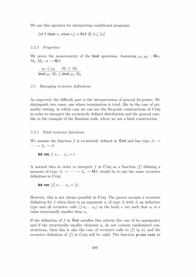
3.3 Managing recursive definitions

As expected, the difficult part is the interpretation of general fix-points. Wedistinguish two cases, one where termination is total, like in the case of pri-mality testing, in which case we can use the fix-point constructions of Coqin order to interpret the recursively defined distribution and the general case,like in the example of the Random walk, where we use a limit construction.

3.3.1 Total recursive functions

We assume the function f is recursively defined in Rml and has type β1 →· · · → βn → β.

let rec f x1 . . . xn = e

A natural idea in order to interpret f in Coq as a function [f ] defining ameasure of type β1 → · · · → βn → Mβ, would be to use the same recursivedefinition in Coq:

let rec [f ]x1 . . . xn = [e]

However, this is not always possible in Coq. The prover accepts a recursivedefinition for f when there is an argument xi of type βi with βi an inductivetype and all recursive calls (f a1 . . . an) in the body e are such that ai is avalue structurally smaller than xi.

If the definition of f in Rml satisfies this criteria (for one of its arguments)and if the structurally smaller elements ai do not contain randomized con-structions, then this is also the case of recursive calls to [f ] in [e] and therecursive definition of [f ] in Coq will be valid. The function prime test in

589

section 2.6 gives an example of this case: it is a structural recursion on thevariable n.

Another important case of recursive definitions in Coq is the case of well-founded recursive definitions. We assume given a relation ≺ on one of thearguments xi of type βi which is proved to be well-founded and such that allrecursive calls (f a1 . . . an) in the body e are such that ai is a non randomizedconstruction and ai ≺ xi is provable. Such that the Coq definition of [f ] usingwell-founded recursion is also valid.

3.3.2 Limit of distributions

In order to interpret recursive functions in which recursive calls are not obvi-ously terminating as in the previous cases, we need to take limits of sequencesof distributions.

As mentioned in section 3.1.1, there is a ω-cpo structure on the functionaltype Mβ = (β → [0, 1])

m→ [0, 1], it is not difficult to show that the least-upperbound operation preserves the measure stability properties, such that the setdistr β is also an ω-cpo.

3.3.3 Fix-points

For the sake of clarity, this explanation is restricted to unary recursive defini-tions; the n-ary case is handled similarly. Let us consider we want to define afunction which satisfies the equation

let rec f x = e

where f is assumed to take an argument in type α, and returns a random valueof type β, such that it has type α→ β and [f ] will have type α→ Mβ. We in-troduce F of type (α→ Mβ)→ α→ Mβ defined by (fun [f ]⇒ fun x⇒ [e]).We assume F to be monotonic: h ≤ g ⇒ F h ≤ F g. Using the ω-cpo structureon α → Mβ, we construct the fix-point fixF of type α → Mβ, this functionwill be our interpretation of f .

As mentioned in section 3.1.1, the inequality fixF x ≤ F (fixF )x holds. Theequality is only provable when F is continuous.

We have proven lemmas stating that the bind operation seen as a monotonicfunction of type distr A

m→ (A → distr B)m→ distr B is continuous.

We have also that the fixpoint operation seen as a monotonic function fromD

c→ D to D is continuous with Dc→ D the set of continuous functions

from D to D. We can deduce (as a meta-theorem that we did not formalize)

590

that functionals generated from Rml expressions will satisfy the continuityhypothesis.

To summarize this section, when a recursive function is introduced in Rmlusing the declaration:

let rec f x = e

we interpret it as a function [f ] defined in our meta-language by

let rec [f ] x = fix (fun [f ]m⇒ fun x⇒ [e]) x

We will explain in the next section how to prove properties of such programs.

4 Derived rules for reasoning on programs

As far as fix-points are concerned, well founded recursive definitions are dealtwith as usual in Coq, and need no further development in this article. Inthis section, we develop an extended axiomatic semantics for Rml programs(section 4.1), with some particular attention to general recursive definitions.Actually, the very novelty when considering some probabilistic program e isthe fact that e may not terminate on every initial state, but rather terminatesalmost surely, which is is a weaker property. From the operational point ofview, this property expresses that e will terminate eventually. This is developedfurther in section 4.4.

4.1 Extending Kozen’s minoring derivation rules

For reasoning about programs, it is convenient to use an axiomatic seman-tics that provides rules by induction on the structure of the program, statingas usual, how some post-condition is satisfied after execution, provided someprecondition holds. In fact, in the context of probabilistic programs, we areinterested (see also (Kozen, 1983)) in deriving some information on the prob-ability for a certain property to hold. Given e : β, its monadic interpretation[e] : Mβ is meant to represent a measure on β, which computes for a functionf : β → [0, 1], its expectation [e]f ∈ [0, 1]. (Usually f will be the character-istic function IP of some predicate P of type β → bool, in which case [e]IPcomputes the probability for the property P .)

The expression [e]f computes the exact expectation, while in general it would

591

be easier to reason on approximation of this value that will be given by apossible interval of values.

Obviously, 0 6 [e]f 6 1 is the worst surrounding we can get for this expec-tation. Whenever [e]I = 1, we understand that [e] is a probability, which alsomeans that e terminates almost surely . On the contrary, the obvious meaningof [e]I = 0 is that e diverges almost surely . Besides these particular cases, weexpect to derive a 6 [e]f 6 b framings, where a 6 b ∈ [0, 1], that is to say[e]f ∈ [a, b]. Therefore, our precondition is going to be some interval I ⊆ [0, 1].

Post-conditions should be similar, but expected to depend on the value re-turned from the computation of e, since we are dealing with functional pro-grams. Thus, post-conditions are taken to be interval-valued functions F , suchthat ∀x : A,F x ⊆ [0, 1].

As a matter of consequence, we provide rules for deriving judgements of theform [e]F ⊆ I, which extends Kozen’s k ≤ [e]f rules (where k ∈ [0, 1], e isan expression of type β and f is a function of type β → [0, 1]) in a consistentway:

The minoration k ≤ [e]f is rewritten as k 6 [e]f ∧ [e]I 6 1, owing to the factthe interpretation [e] is monotonic.

Before going through the details, let us notice that this presentation could havebeen settled in the usual Scott’s domains framework (Scott, 1972), where theset I of intervals included in [0, 1] is turned into an ω-cpo, with ordering theconverse of inclusion, [0, 1] as bottom element and intersection as the leastupper-bound operation. As a matter of fact, if we do not restrict ourselves tothe unit interval, this is Scott’s Interval Domain, which is the interpretationfor abstract data type R in his model for functional programming. We do notneed to deal with the full presentation for our purpose, but for two importantpoints. First of, maximal elements of the Interval Domain are singleton setsr ≡ [r, r], where r ∈ R. In our framework, maximal elements are the same,restricted to r ∈ [0, 1], and are associated (obviously) to equality proofs. Inother words, maximal interval matches the best information we can derive forsome probability, while [0, 1] matches the worst, useless information. Secondly,we have to cope with recursive definitions, in which case we shall need mono-tonic interval sequences (In)n such that for all n, In+1 ⊆ In. Then, the leastupper bound ∩nIn is well defined. This is going to be sufficient in this setting.

4.2 Definition on intervals

An interval I is given by its lower bound low I and its upper bound up I suchthat 0 ≤ low I ≤ up I ≤ 1, and we write it [low I, up I], we use the notation

592

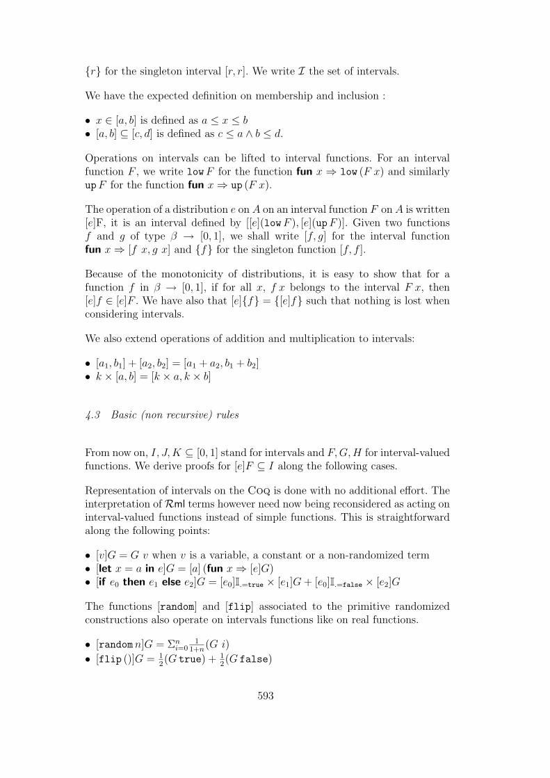
r for the singleton interval [r, r]. We write I the set of intervals.

We have the expected definition on membership and inclusion :

• x ∈ [a, b] is defined as a ≤ x ≤ b• [a, b] ⊆ [c, d] is defined as c ≤ a ∧ b ≤ d.

Operations on intervals can be lifted to interval functions. For an intervalfunction F , we write lowF for the function fun x ⇒ low (F x) and similarlyupF for the function fun x⇒ up (F x).

The operation of a distribution e on A on an interval function F on A is written[e]F, it is an interval defined by [[e](lowF ), [e](upF )]. Given two functionsf and g of type β → [0, 1], we shall write [f, g] for the interval functionfun x⇒ [f x, g x] and f for the singleton function [f, f ].

Because of the monotonicity of distributions, it is easy to show that for afunction f in β → [0, 1], if for all x, f x belongs to the interval F x, then[e]f ∈ [e]F . We have also that [e]f = [e]f such that nothing is lost whenconsidering intervals.

We also extend operations of addition and multiplication to intervals:

• [a1, b1] + [a2, b2] = [a1 + a2, b1 + b2]• k × [a, b] = [k × a, k × b]

4.3 Basic (non recursive) rules

From now on, I, J,K ⊆ [0, 1] stand for intervals and F,G,H for interval-valuedfunctions. We derive proofs for [e]F ⊆ I along the following cases.

Representation of intervals on the Coq is done with no additional effort. Theinterpretation of Rml terms however need now being reconsidered as acting oninterval-valued functions instead of simple functions. This is straightforwardalong the following points:

• [v]G = G v when v is a variable, a constant or a non-randomized term• [let x = a in e]G = [a] (fun x⇒ [e]G)• [if e0 then e1 else e2]G = [e0]I.=true × [e1]G+ [e0]I.=false × [e2]G

The functions [random] and [flip] associated to the primitive randomizedconstructions also operate on intervals functions like on real functions.

• [randomn]G = Σni=0

11+n

(G i)

• [flip ()]G = 12(G true) + 1

2(G false)

593

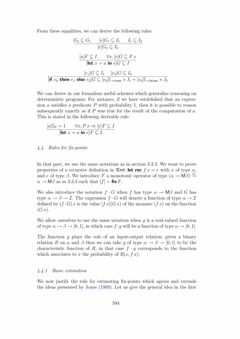
From these equalities, we can derive the following rules:

G2 ⊆ G1 [e]G1 ⊆ I1 I1 ⊆ I2[e]G2 ⊆ I2

[a]F ⊆ I ∀x, [e]G ⊆ F x

[let x = a in e]G ⊆ I

[e1]G ⊆ I1 [e2]G ⊆ I2[if e0 then e1 else e2]G ⊆ [e0]I.=true × I1 + [e0]I.=false × I2

We can derive in our formalism useful schemes which generalize reasoning ondeterministic programs. For instance, if we have established that an expres-sion a satisfies a predicate P with probability 1, then it is possible to reasonsubsequently exactly as if P was true for the result of the computation of a.This is stated in the following derivable rule:

[a]IP = 1 ∀x, P x⇒ [e]F ⊆ I

[let x = a in e]F ⊆ I

4.4 Rules for fix-points

In that part, we use the same notations as in section 3.3.3. We want to proveproperties of a recursive definition in Rml: let rec f x = e with x of type α,and e of type β. We introduce F a monotonic operator of type (α→ Mβ)

m→α→ Mβ as in 3.3.3 such that [f ] = fixF .

We also introduce the notation f · G when f has type α → Mβ and G hastype α → β → I. The expression f · G will denote a function of type α → Idefined by (f ·G)x is the value [f x](Gx) of the measure (f x) on the function(Gx).

We allow ourselves to use the same notation when g is a real-valued functionof type α→ β → [0, 1], in which case f ·g will be a function of type α→ [0, 1].

The function g plays the role of an input-output relation: given a binaryrelation R on α and β then we can take g of type α → β → [0, 1] to be thecharacteristic function of R, in that case f · g corresponds to the functionwhich associates to x the probability of R(x, f x).

4.4.1 Basic estimation

We now justify the rule for estimating fix-points which agrees and extendsthe ideas presented by Jones (1989). Let us give the general idea in the first

594

place. The Rml definition let rec f x = e for f can also be considered as thefix-point of some functional F such that [f ]x = fixF x.

Given the interval-valued function G, we want to estimate [f x]G, so to findI such that [f x]G ⊆ I. The maximal interval I = [0, 1] is a trivial solution.Now the fix-point is the result of the iteration of the functional F , so if it ispossible to decrease the interval at each step, we can deduce an approximationfor f .

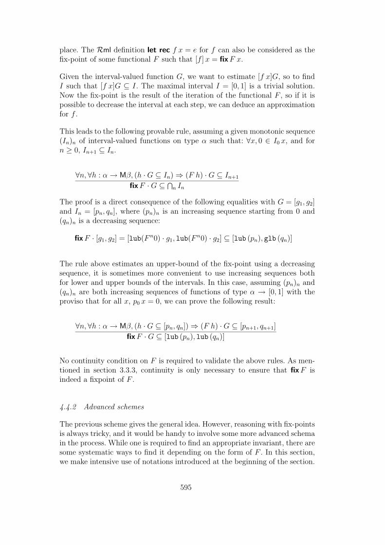
This leads to the following provable rule, assuming a given monotonic sequence(In)n of interval-valued functions on type α such that: ∀x, 0 ∈ I0 x, and forn ≥ 0, In+1 ⊆ In.

∀n,∀h : α→ Mβ, (h ·G ⊆ In)⇒ (F h) ·G ⊆ In+1

fixF ·G ⊆ ⋂n InThe proof is a direct consequence of the following equalities with G = [g1, g2]and In = [pn, qn], where (pn)n is an increasing sequence starting from 0 and(qn)n is a decreasing sequence:

fixF · [g1, g2] = [lub(F n0) · g1, lub(F n0) · g2] ⊆ [lub (pn), glb (qn)]

The rule above estimates an upper-bound of the fix-point using a decreasingsequence, it is sometimes more convenient to use increasing sequences bothfor lower and upper bounds of the intervals. In this case, assuming (pn)n and(qn)n are both increasing sequences of functions of type α → [0, 1] with theproviso that for all x, p0 x = 0, we can prove the following result:

∀n,∀h : α→ Mβ, (h ·G ⊆ [pn, qn])⇒ (F h) ·G ⊆ [pn+1, qn+1]

fixF ·G ⊆ [lub (pn), lub (qn)]

No continuity condition on F is required to validate the above rules. As men-tioned in section 3.3.3, continuity is only necessary to ensure that fixF isindeed a fixpoint of F .

4.4.2 Advanced schemes

The previous scheme gives the general idea. However, reasoning with fix-pointsis always tricky, and it would be handy to involve some more advanced schemain the process. While one is required to find an appropriate invariant, there aresome systematic ways to find it depending on the form of F . In this section,we make intensive use of notations introduced at the beginning of the section.

595

In this part, we took inspiration from the loop rules in pGCL introduced byMorgan (as described in McIver and Morgan (2005)) and propose a systematicgeneralization to the case of recursive functions.

Let us make some preliminary observations. We start from a recursive defini-tion let rec f x = e on type α→ β. Assuming f is deterministic and we wantto prove that ∀x, P (f x), a natural approach is to try to find an inductiveargument which shows that the body e of the function f satisfies P assumingthe recursive calls in e do. More formally, if the definition f corresponds to thefunctional F , we can try to prove for an arbitrary function h that, ∀x, P (hx)implies ∀x, P (F hx).

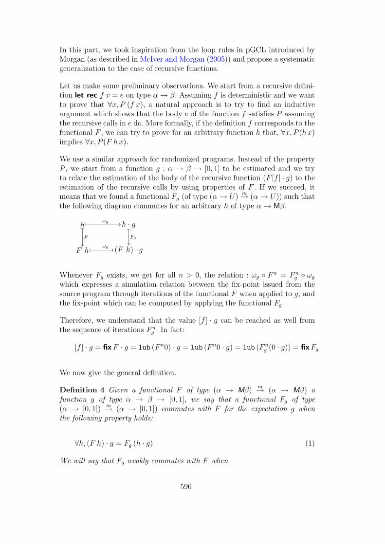
We use a similar approach for randomized programs. Instead of the propertyP , we start from a function g : α → β → [0, 1] to be estimated and we tryto relate the estimation of the body of the recursive function (F [f ] · g) to theestimation of the recursive calls by using properties of F . If we succeed, itmeans that we found a functional Fg (of type (α→ U)

m→ (α→ U)) such thatthe following diagram commutes for an arbitrary h of type α→ Mβ.

h_

F

ωg //h · g_

Fg

F h ωg // (F h) · g

Whenever Fg exists, we get for all n > 0, the relation : ωg F n = F ng ωg

which expresses a simulation relation between the fix-point issued from thesource program through iterations of the functional F when applied to g, andthe fix-point which can be computed by applying the functional Fg.

Therefore, we understand that the value [f ] · g can be reached as well fromthe sequence of iterations F n

g . In fact:

[f ] · g = fixF · g = lub (F n0) · g = lub (F n0 · g) = lub (F ng (0 · g)) = fixFg

We now give the general definition.

Definition 4 Given a functional F of type (α → Mβ)m→ (α → Mβ) a

function g of type α → β → [0, 1], we say that a functional Fg of type(α → [0, 1])

m→ (α → [0, 1]) commutes with F for the expectation g whenthe following property holds:

∀h, (F h) · g = Fg (h · g) (1)

We will say that Fg weakly commutes with F when

596

∀h, (F h) · g ≤ Fg (h · g) (2)

An important consequence of the existence of Fg is that the estimation ofexpectation for the fix-point can be related to the fix-point of Fg as stated inthe following lemma.

Proposition 5 Given a real-valued function g of type α → β → [0, 1] and amonotonic operator Fg of type (α→ [0, 1])

m→ (α→ [0, 1]):

• if Fg weakly commutes with F for g then fixF · g ≤ fixFg.• if Fg commutes with F for g then fixF · g = fixFg.

Now we can use the fact that fixFg is an initial fix-point, such that if we canfind a real-valued function φ of type α → [0, 1] such that Fg φ ≤ φ then wededuce fixFg ≤ φ and combining this result with the last property, we obtainthe following result:

Proposition 6 Given a real function g of type α → β → [0, 1] such thatthere exists a monotonic operator Fg which weakly commutes with F for g, ifFg φ ≤ φ then fixF · g ≤ φ.

In most cases, we also want a minoration for fixF · g. For that, we have toreverse this result and consider how the distribution fixF operates on 1−g.

Proposition 7 Given a real function g of type α→ β → [0, 1] such that thereexists a monotonic operator F1−g which weakly commutes with F for 1−g, ifF1−g (1−φ) ≤ (1−φ) then φ & (fixF · I) ≤ fixF · g.

The function fixF · I associates to each x the probability that the recursivefunction terminates on x.

PROOF. The value x & y is defined in our formalism as 1−((1−x) + (1−y))using our bounded addition and corresponds to the real max(0, x+ y − 1). Inparticular x & 1 = x so for any function f , f & I = f .

The proof uses the fact that for any distribution µ of type Mβ, we have(1−µ(1−h1)) & µ(h2) ≤ µ(h1 & h2). From the previous proposition appliedto 1−φ we have fixF · (1−g) ≤ 1−φ. so φ ≤ 1−fixF · (1−g) then:

φ & (fixF · I) ≤ (1−fixF · (1−g)) & (fixF · I)

≤ fixF · (g & I) = fixF · g

There is a special case where we can get a minoration by φ, this is when

597

φ ≤ fixF ·I which can be seen as a generalisation of the fact that our invariantestimation φ implies termination of the fix-point. In order to obtain this result,we need (fixF · I)− φ to be a pre-fixpoint of F1−g.

Proposition 8 Let g be a real function of type α→ β → [0, 1] such that thereexists a monotonic operator F1−g which weakly commutes with F for 1−g. Ifthe properties F1−g ((fixF · I)− φ) ≤ (fixF · I)− φ and φ ≤ fixF · I hold, thenφ ≤ fixF · g.

PROOF. This results is obtained using the previous proposition with theinvariant φ′ = φ + 1−(fixF · I). We have 1−φ′ = (fixF · I) − φ such thatF1−g (1−φ′) ≤ 1−φ′ by hypothesis, consequently φ′ & fixF · I ≤ fixF · g.

The final result comes from properties of + and & on [0, 1]:

φ′ & fixF · I = (φ+ (1−fixF · I ) & fixF · I = φ

4.4.3 Application to loops

We can define recursively a loop function in Rml. We assume given a type Sfor states, a boolean condition cond of type S → bool and a body body oftype S → S.

let rec loop s =

if cond s then let s’ = body s in loop s’ else s

The interpretation [cond] will have type S → Mbool and [body] will have typeS → MS.

We introduce the terms ctrue s = [cond s]I.=true and cfalse s = [cond s]I.=false

We want to measure a function g of type S → [0, 1] on the output state ofloop, which does not depend on the input state. We still use the notation f ·gin place of the more verbose f · fun s⇒ g.

We write F for the functional associated to loop. We have:

(F f) · g = fun s⇒ (ctrue s)× [body s](f · g) + (cfalse s)× (g s)

Such that the functional Fg which commutes with F for g can be defined thefollowing way:

Fg h = fun s⇒ (ctrue s)× [body s]h+ (cfalse s)× (g s)

598

It is easy to check the following property : F1−g (1−h) ≤ 1−(Fg h) such thatthe condition φ ≤ Fg φ is sufficient to ensure F1−g (1−φ) ≤ 1−φ. And we canderive the following theorem :

Proposition 9 Given g, φ and ψ of type S → [0, 1],assuming ∀s, φ s ≤ (ctrue s)× [body s]φ+ (cfalse s)× (g s)and ∀s, (ctrue s)× [body s]ψ + (cfalse s)× (g s) ≤ ψ swe can deduce φ & [loop] · I ≤ [loop] · g ≤ ψ

In case cond is a non randomized construction, let C s be the property cond s =true. The condition:φ s ≤ (ctrue s)× [body s]φ+ (cfalse s)× (g s) becomes:C s⇒ φ s ≤ [body s]φ and ¬C s⇒ φ s ≤ g swhich is a generalization of the loop rule in axiomatic semantics, φ being theinvariant which should be preserved in the body (when the condition is true)and should establish the post-condition at the end (when the condition isfalse).

We consequently have the following rule which corresponds to the total loopcorrectness rule in McIver and Morgan (2005):

∀s, C s⇒ φ s ≤ [body s]φ

∀s, φ s & [loop s]I ≤ [loop s](φ & I¬C)

5 Applications

We apply our approach for proving properties of simple randomized programs.

5.1 Probabilistic termination

We return to our example of section 2.6.2, a random walk which illustratesprobabilistic termination.

let rec walk x = if flip() then x else walk (x+1)

We show that this program terminates with probability one. For that it isenough to prove that:

∀x, [walkx]I = 1.

599

The functional F to be considered is:

fun [walk]m⇒ fun x⇒ [if flip() then x else walk (x+ 1)]

when w : nat→ Mnat, x : nat and g : nat→ [0, 1] to be measured, we have:

(F w · g)x =1

2(g x) +

1

2(w · g) (x+ 1)

We can introduce Fg of type (nat→ [0, 1])m→ (nat→ [0, 1]) such that

Fg hx =1

2g x+

1

2(h (x+ 1))

and check the commutation property between Fg and F .

In case g is the function I we get the functional

FI hx =1

2+

1

2(h (x+ 1))

we know by proposition 5 that

[walkx]I = fixFI x

what remains to be computed is fixFI x.

The real fixFI x is the least-upper bound of a sequence (pi)i such that p0 = 0and pi+1 = 1

2+ 1

2pi.

It is easy to show that pn = 1− 12n , that the least upper bound of the sequence

(pi)i is 1 such that fixFI x = lub(pn)n = 1.

5.2 Parametrized termination

This example is taken from Ycart (2002), adapted here to fit with our restric-tion to discrete random distributions. It can be seen as a generalisation ofwalk where the probability to stop or continue is given in each point by anarbitrary function K x.

We assume given a non-randomized function K of type nat → nat and aninteger N . We write also Y x for the element of [0, 1] defined as (K x)/1 +N .

600

The function we want to study is defined by the following Rml program:

let rec ω x = if randomN < K x then x else ω (x+ 1)

We have [ω] = fix F , where F f x ≡ [if randomN < K x then x else f (x+1)].

Let us start with some informal observations. Given θ : nat → [0, 1], assumewe want to approximate the value of [ω x]θ ∈ [0, 1]. From a mathematicalpoint of view, this is a summation. Let us have a naive look at it:

∫θ(y)d[ω x](y) = (Y x)θ x+ (1−(Y x))

∫θ(y)d[ω (x+ 1)](y)

From the section 2.5.5, we know our monadic interpretation expresses thesame idea, in a more formal setting.

5.2.1 Putting advanced schemes at work

[ω x]θ= (Y x)θ x+ (1−(Y x))[ω (x+ 1)]θ

= (Y x)θ x+ (1−(Y x))(Y (x+ 1))θ (x+ 1)

+(1−(Y x))(1−(Y (x+ 1))[ω (x+ 2)]θ

= . . .

= (Y x)× θ x+ · · ·+x+n∏k=x

(1−Y k)[ω (x+ 1 + n)]θ

We observe that the potential source of divergence depends on the behaviourof the infinite product R∞(x), limit of the sequence Rn(x) ≡ ∏x+n−1

k=x (1−Y k).Let us make this observation more formal. Considering the functional F whichdefines the fix-point, we rather get:

[F f x]θ= (Y x)θ x+ (1−(Y x))[f (x+ 1)]θ (3)

This turns out to be an application of the properties presented in section 4.4.2.

From equation 3, we get that the commutation property holds with the func-tional

Fθ hx = (Y x)× (θ x) + (1−Y x)× (h (x+ 1))

When θ is the unit function I, we obtain :

FI hx = (Y x) + (1−Y x)× (h (x+ 1))

601

The proposition 5 ensures that [ω x]I = fixFI x so it remains to compute thisfixpoint, it is the limit of a sequence sn such that s0 x = 0 and sn+1 x =(Y x) + (1−Y x)× (sn (x+ 1)).

One shows by induction on n that

sn x =n−1∑k=0

Y (x+ k)×Rk(x)

with Rn(x) as defined above. then using the fact that Y (x + k) × Rk(x) =Rk(x)−Rk+1(x) we deduce sn x = R0(x)−Rn(x) = 1−Rn(x) and consequentlythe expected limit of sn x is equal to 1−∏∞i=x 1−(Y i). We deduce the expectedresult:

[ω x]I = 1−∞∏i=x

1−(Y i)

We now illustrate the use of other rules for fix-points. We may be interested toshow that the function ω applied on x never outputs value less than x. Becauseit is a property always true, one possibility would be to use the power of theCoq type system and have a semantic which associates to x a distribution onnumbers greater or equal to x. However, if we stay in our Rml framework, wemay want to prove that the probability for ω x to output a value less than x is0, which can be rephrased as [ω x]I.<x = 0. This is a case where the function tobe measured I.<x depends on the input x. With g of type nat→ nat→ [0, 1]we have

(F f · g)x = [F f x](g x) = (Y x)× (g x x) + (1−Y x)× [f (x+ 1)](g x)

We consider g x = I.<x. This does not lead directly to a commutation property,because we need a sub-expression of the form [f (x+ 1)](g (x+ 1)) in order toabstract with respect to the function f · g. We remark that g x x = I.<x x = 0and also that g x = I.<x ≤ I.<x+1 = g (x + 1) such that we have for thisparticular g:

(F f · g)x ≤ (1−Y x)× (f · g) (x+ 1)

and we can introduce the function Fg which weakly-commutes with F

Fg hx = (1−Y x)× (h (x+ 1))

Now we remark that h = 0 is an invariant of Fg such that using proposition 6,we deduce [ω x]I.<x ≤ 0 which is the expected result.

602

We can deduce using the same kind of reasoning that [ω x]I.=x = Y x. Thegeneral method is again to rewrite F f · g for that particular case. We obtainbecause g x x = 1:

(F f · g)x = (Y x) + (1−Y x)× [f (x+ 1)](g x)

now we would like to reuse our previous result which ensures that ω (x +1) · I.=x ≤ ω (x + 1) · I.<x+1 = 0. This is possible using a stronger notion ofcommutation in proposition 5 where we force the variable f to be less thanthe fixpoint we analyse, in our case, we may assume f ≤ [ω] and consequentlyuse [f (x+ 1)](g x) = 0.

We obtain (F f · g)x = (Y x) so the (constant) functional Fg hx = Y x com-mutes with F for g and [ω x]I.=x = fix Fg = Y x.

The lemmas in Coq involving commutation in section 4.4.2 have been devel-oped with this stronger notion of commutation ie ∀h, h ≤ fixF ⇒ F h · g =Fg (h · g).

5.2.2 Some practical consequences

Turning back to our program ω, taking x = 0 as an example, we have provedso far:

∫(I y)d[ω 0](y) = 1−

∞∏k≥0

(1−Y k)

Therefore, the termination depends upon the asymptotic behaviour of Y x =(K x)/1+N , through the existence of the limit R∞(x). For instance, wheneverK is non-zero, (ω 0) terminates almost surely; while if K always returns the 0value, then this program diverges almost surely. If K n = 0 as soon as n ≥ pfor some integer p > 0, then (ω 0) terminates with probability 1−∏p

k=0(1−Y k).

5.3 The Bernoulli distribution

We now apply our technique to the proof of an algorithm to simulate a Booleanfunction following Bernoulli’s distribution (which is true with some probabil-ity p and false with probability 1−p) using only a coin flip. The algorithmwhich is also taken as an example by Hurd (2002a) uses a simple idea : writep in binary form

∑∞i=1 pi

12i , if we flip a coin and get a sequence (qi)i≥1 then

the first time we get qi 6= pi, we answer true when qi < pi and false otherwise.Now this function can be expressed recursively. If p < 1

2then p1 = 0 and the

603

remainder of the sequence corresponds to 2× p = p+ p. If 12≤ p then p1 = 1

and the remainder of the sequence corresponds to 2 × p − 1 = p & p (usingthe special operation x & y we introduced in section 3.1.5). Our Bernoulliprogram can be written as

let rec bernoulli p =

if flip() then if p < 12

then false else bernoulli (p & p)

else if p < 12

then bernoulli (p + p) else true

As before, given a function g of type bool → [0, 1] (not depending on theinput p of the function), we compute the value of the functional F associatedto bernoulli:

[F f p]g = if p < 12

then 12(g false) + 1

2[f (p+ p)]g

else 12[f (p & p)]g + 1

2(g true)

So Fg commutes with F for g with Fg defined by:

Fg h p = if p < 12

then 12(g false) + 1

2(h (p+ p))

else 12(h (p & p)) + 1

2(g true)

In case g is the function I, we have

FI h p = if p < 12

then 12

+ 12(h (p+ p)) else 1

2(h (p & p)) + 1

2

In order to compute fixFI we introduce the sequence p0 = 0 pn+1 = 12

+ 12pn,

which is the same sequence we used for the termination of walk, its limit is 1.

So we know that bernoulli terminates almost surely ie fixF · I = 1 weconsequently can use propositions 6 and 7 in order to study the probability ofthe result to be true.

With g = I.=true we have

Fg h p= if p < 12

then 12h (p+ p) else 1

2h (p & p) + 1

2

F1−g h p= if p < 12

then 12

+ 12h (p+ p) else 1

2h (p & p)

We take for invariant φ p = p, in order to deduce fixF p · I.=true = p it isenough to prove that φ is a pre fix-point of Fg (ie Fg φ ≤ φ) and 1−φ is apre fix-point of F1−g (ie F1−g (1−φ) ≤ 1−φ). So we simply have to prove thefollowing properties which are consequences of properties of [0, 1]:

• if p < 12

then 12(p+ p) else 1

2(p & p) + 1

2≤ p

604

• if p < 12

then 12

+ 12(1−(p+ p)) else 1

2(1−(p & p)) ≤ 1−p

5.4 Improving precision

The previous examples show the proof of properties of particular programs.Our Coq development gives us the possibility to also derive more abstractproperties involving program schemes.

We study a program scheme where a randomized program is executed twicein order to improve the probability of getting a correct result. The implicitassumption is that given two runs on the program we can choose the better ofthe two answers. In case of primality for instance, if one of the tests answersthat p is not prime, we are sure that p is not prime; only when the two programsassert that p is prime, we can still pretend (but with higher confidence) thatp is prime.

We want to compute a value in a type β which satisfies a property Q with acertain probability. The hypotheses are that we have two programs p1 and p2

of type β, thus interpreted as objects of type Mβ. We want to combine p1 andp2 in order to get a better program i.e. we want to improve the probabilitythat the result is correct.

We assume we have a non-randomized function choice of type β → β → βsuch that (Q x)⇒ Q (choicex y) and (Q y)⇒ Q (choicex y) are provable.

In case of a Boolean test for primality of p, we have (Q b) defined as (b =true ⇒ p is prime) and (choice b1 b2) defined as (b1 and b2). The oppositedirection p is prime ⇒ b = true is always satisfied for the output of theprogram so does not require further analysis.

Now we build a new program p:

let x = p1 in let y = p2 in choice x y

We assume that we have estimations for the probability of p1 (resp p2) tosatisfy Q, ie k1 ≤ [p1]IQ (resp. k2 ≤ [p2]IQ) and we want to prove that theprogram p satisfies Q with a better probability.

Let k stands for the expression k1 +k2−k1k2, and notice that k = k1(1−k2) +k2 = k2(1−k1) + k1 such that k is greater than both k1 and k2.

We are going to show that k1 ≤ [p1]IQ and k2 ≤ [p2]IQ implies k ≤ [p]IQ.

Actually we establish a more general result, using an arbitrary function q of

605

type β → [0, 1] instead of the characteristic function IQ of a predicate Q. Weassume that ∀x y, (q x)+(q y) ≤ q (choicex y) (with bounded addition). It iseasy to see that when q is the characteristic function IQ, then the assumptions(Q x)⇒ Q (choicex y) and (Q y)⇒ Q (choicex y) are equivalent to (IQ x)+(IQ y) ≤ IQ (choicex y). We also need the fact that both programs p1 and p2

terminate with probability one, otherwise our choice function could give aresult which is not as good as p1 and p2. Now, the property to be shownamounts to

k ≤ [p1] (fun x⇒ [p2] (fun y ⇒ q (choicex y)))

Using the fact that

(q x)× (1−q y) + q y ≤ q x+ q y ≤ q (choicex y)

the proof reduces to

k ≤ [p1](fun x⇒ [p2](fun y ⇒ (q x)× (1−q y) + q y))

Algebraic properties of measures lead to simplification of the right-hand side:

[p1]q × [p2](1−q) + [p2]q

Because p2 terminates, we have [p2](1−q) = 1−[p2](q) (only the inequality istrue in general) so we have to show:

k1(1−k2) + k2 ≤ [p1]q × (1−[p2]q) + [p2]q

which is true because k is, by construction, monotonic with respect to bothk1 and k2.

This example illustrates the possibility to do abstract modular reasoning inour framework. In Coq, the expressions [p1] and [p2] are just represented asvariables of type Mβ.

6 Related work

Park et al. (2005) propose a probabilistic functional language, named λ© whichextends the ML functional kernel on the basis of the monadic metalanguagedeveloped by Pfenning and Davies (2001). A key feature is the clear syntacti-cal separation between deterministic terms and probabilistic expressions. The

606

latter correspond to mathematical random variables. Any term can be seen asan expression : the Dirac mass distribution on this term. From any expressionE, the operator prob E builds the associated image measure. As for randomprimitives, the language introduces the constant expression S which denotesa random variable following the uniform law on [0, 1]. In Rml, one does notdistinguish between these two syntactic categories; the monadic transforma-tion forces any Rml term into a measure of some kind. The monadic opera-tors unit and bind get as close as possible from the corresponding prob andsample x from · · · in · · · from λ©.

The language λ© is mainly designed toward expressiveness as a programminglanguage, for which the paper provides a small steps operational semantics.This corresponds to Kozen’s first semantics in Kozen (1981), where any com-putation involved in a reasoning step about a program requires the user torefer to the measurable space of random streams over [0, 1]. As far as reasoningon programs is concerned, this is not of great help, since axiomatic semanticsrelies on denotational semantics instead. Therefore, examples developed withλ© are better analysed through simulation techniques. These approaches arecomplementary: we are not able to simulate the programs as sampling func-tions but we can directly and easily reason on the probabilistic properties of(a subset of) O’Caml expressions.

In this paper, we have limited ourselves to discrete distributions, with the ben-efit of ensuring our monadic transformation to interpret properly programs asmathematical measures. We think the continuous case could be reached, start-ing from the formal development done so far with the U axiomatization, butthis point requires further investigations. The current presentation does nottake measurability property into account. This is not required in the discretecase, but cannot be ignored in the general case anymore. We strongly con-sider Jones and Plotkin (1989) work as a possible direction to follow, provid-ing that the interpretation of type β is given a cpo-structure. Also the recentwork by Hasan and Tahar (2007), which develops a formalization of continuousprobability distributions based on Hurd’s approach, deserves interest towardsthis goal.

McIver and Morgan (2005) describe an axiomatic semantics for probabilisticprograms written in imperative style. The state-predicates in Hoare logic arereplaced by so-called expectations which are functions from states to R+, tobe evaluated according to the distribution defined by the program. An impor-tant aspect of this work is to introduce in the language a non-deterministic(demonic) choice p u q. The probability for a property P to hold after exe-cuting p u q is the minimum of the probabilities that P holds after execut-ing p and after executing q. This operator is used to represent specificationsand for defining a refinement relation. In order to adapt our approach tothe non-deterministic case, an idea could be to relax the compatibility condi-

607

tion for addition in the definition of a distribution into the weaker conditionµ(f) + µ(g) ≤ µ(f + g). Developing the corresponding theory still remainsto be done. A mechanization of this calculus using the HOL theorem proveris presented in Hurd et al. (2005). In this work programs are interpreted asfunctionals of type (α→ R+

∞)→ (α→ R+∞) where R+

∞ ≡ R+ ∪ ∞ and α isthe type of states. A so-called deep-embedding is proposed. The syntax of thelanguage of guarded commands and the weakest-precondition generator areexplicitly encoded in the proof assistant. Our approach uses instead a shallowembedding where we directly encode the semantics of the language. Also, theirapproach allows to measure an arbitrary (measurable) R+-valued function; Wechoose to restrict ourselves to [0, 1]-valued ones in order to simplify the formaldevelopment in Coq and because it is sufficient for correctness. Measuringarbitrary function can nevertheless be interesting in some cases. For instance,in the random walk example, one could measure the average of the result ofthe function (how many flips before we get false). We plan to investigate howto extend our development in that direction.

As already said in the introduction, our approach owes much to Kozen aswell as to Hurd’s thesis, where formal verification of probabilistic programs ishandled with the HOL theorem prover. Hurd uses a monadic translation basedon a global state with a stream of boolean values. Reasoning on programsrequired to define within HOL an adequate distribution over this infinitestructure, while we only use simple mathematical constructions. It would beinteresting to compare more carefully the complexity of proofs of high-levelprograms in both systems.

7 Conclusion

We have studied the interpretation of probabilistic programs in a functionalframework using a monadic interpretation of programs as probability distri-butions represented by measures.

We have applied this technique for building an environment for reasoningabout probabilistic programs in the Coq proof assistant. We have developedan axiomatization for the set [0, 1] which uses a few primitive operations :bounded addition, multiplication, inverse (1−x), least upper-bounds of mono-tonic sequences.

We have derived axiomatic rules for estimating the probability that programssatisfy some given properties, following the structure of the program. Whendealing with probabilistic termination of programs, we provide several fix-point rules, which could cover a wide class of situations. We provide few basicexamples for showing how to take benefit of them. The development and

608

results presented in this paper have been formally derived and checked inthe Coq proof assistant and are available as a contribution (Paulin-Mohring,2007).

Futher research topics concern both theoretical issues and more practical con-cerns. On the former side, we want to deepen the relations between the [0, 1]-segment of R which is formalized by our axiomatization type U and otheraxiomatizations for the reals studied elsewhere. We are also interested in theapproach taken by Escardo and Simpson (2001) in the development of RealPCF. See also Geuvers et al. (2007) for a quite comprehensive survey.

On the other side, we plan the development of an environment for analysingrandomized functional programs. Basically, the tool should automatically gen-erate verification conditions from the specification of pre and post conditionsplus a validation (the correctness proof in Coq obtained from the monadictranslation of the program). This gets close to design infrastructure offeredby the Why tool (Filliatre, 2002, 2003), with the consequence of allowingeventually other prover assistants as well for the logical backend.

We are also looking forward to more advanced examples that certainly willrequire more challenging automation of their proofs.

Acknowledgments We thank A. McIver and C. Morgan for useful commentson the first version of this paper and the referees for pointing out inaccuraciesin an early version of this paper. We also thank R. Lassaigne for stimulatingdiscussions on formal proofs for analyzing random programs and P. Lescannefor his feedback on the introduction part.

References

Audebaud, P., Paulin-Mohring, C., 2006. Proofs of randomized algorithmsin Coq. In: Uustalu, T. (Ed.), Mathematics of Program Construction,MPC’2006. Vol. 4014 of Lecture Notes in Computer Science. Springer-Verlag, Kuressaare, Estonia, pp. 49–68.

Escardo, M., Simpson, A., 2001. A universal characterization of the closed eu-clidean interval (extended abstract). In: IEEE Symp. on Logic in ComputerScience. Boston, Massachusetts, pp. 115–125.

Filliatre, J.-C., 2002. The Why verification tool.URL http://why.lri.fr/

Filliatre, J.-C., Jul. 2003. Verification of Non-Functional Programs using Inter-pretations in Type Theory. J. of Functional Programming 13 (4), 709–745.

Geuvers, H., Niqui, M., 2002. Constructive reals in Coq: Axioms and cate-goricity. In: Callaghan, P., Luo, Z., McKinna, J., Pollack, R. (Eds.), Types

609

for Proofs and Programs. Selected Papers. Vol. 2277 of Lecture Notes inComputer Science. Springer-Verlag, pp. 79–95.

Geuvers, H., Niqui, M., Spitters, B., Wiedijk, F., 2007. Constructive analy-sis, types and exact real numbers. Mathematical Structures in ComputerScience 17 (1), 3–36.

Giry, M., 1982. A categorical approach to probability theory. In: Banaschewski,B. (Ed.), Categorical Aspects of Topology and Analysis. Vol. 915 of LectureNotes in Mathematics. pp. 69–85.

Hasan, O., Tahar, S., 2007. Formalization of continuous probability distribu-tions. In: Proc. 21st Conference on Automated Deduction (CADE-21). Vol.4603 of Lecture Notes in Artificial Intelligence. Springer-Verlag, pp. 3–16.

Hurd, J., 2002a. A formal approach to probabilistic termination. In: Carreno,V. A., Munoz, C. A., Tahar, S. (Eds.), Theorem Proving in Higher OrderLogics. Vol. 2410 of Lecture Notes in Computer Science. Springer-Verlag,Hampton, VA, USA, pp. 230–245.

Hurd, J., 2002b. Formal verification of probabilistic algorithms. Ph.D. thesis,Univ. of Cambridge.

Hurd, J., 2003. Verification of the Miller-Rabin probabilistic primality test.J. of Logic and Algebraic Programming 50 (1–2), 3–21, special issue onProbabilistic Techniques for the Design and Analysis of Systems.

Hurd, J., McIver, A., Morgan, C., 2005. Probabilistic guarded commandsmechanized in HOL. In: Cerone, A., Pierro, A. D. (Eds.), Quantitative As-pects of Programming Languages. Vol. 112 of ENTCS. Elsevier, Barcelona,Spain, pp. 95–111.

Jones, C., 1989. Probabilistic non-determinism. Ph.D. thesis, Univ. of Edin-burgh.

Jones, C., Plotkin, G., 1989. A probabilistic powerdomain of evaluations. In:Proceedings of the Fourth Annual Symposium on Logic in computer science.IEEE Press, Piscataway, NJ, USA, pp. 186–195.

Kozen, D., 1981. Semantics of probabilistic programs. J. of Computer andSystem Science 22, 328–350.

Kozen, D., 1983. A probabilistic pdl. In: STOC ’83: Proceedings of the fifteenthannual ACM symposium on Theory of computing. ACM Press, New York,NY, USA, pp. 291–297.

Lawvere, F. W., 1962. The category of probabilistic mappings, preprint.McIver, A., Morgan, C., 2005. Abstraction, Refinement and Proof for Proba-

bilistic Systems. Monographs in Computer Science. Springer-Verlag.Moggi, E., 1991. Notions of computation and monads. Information and Com-

putation 93 (1), 55–92.Morgan, C., McIver, A., 1999. pGCL: formal reasoning for random algorithms.

South African Computer Journal 22, 14–27.Park, S., Pfenning, F., Thrun, S., 2005. A probabilistic language based upon

sampling functions. In: ACM Symp. on Principles of Programming Lan-guages. pp. 171–182.

Paulin-Mohring, C., Jan. 2007. A library for reasoning on randomized algo-

610

rithms in Coq. Description of a Coq contribution, INRIA & Univ. ParisSud.URL http://www.lri.fr/~paulin/ALEA/library.pdf

Pfenning, F., Davies, R., 2001. A judgmental reconstruction of modal logic.Mathematical Structures in Computer Science 11 (4), 511–540.

Ramsey, N., Pfeffer, A., 2002. Stochastic lambda calculus and monads of prob-ability distributions. In: Mitchell, J. (Ed.), ACM Symp. on Principles ofProgramming Languages. pp. 154–165.

Scott, D., 1972. Lattice theory, data types, and semantics. In: Rustin, R. (Ed.),Formal Semantics of Programming Languages. Vol. 2 of Courant ComputerScience Symposia. pp. 65–106.

Ycart, B., 2002. Modeles et algorithmes markoviens. No. 39 in Collection SMAIMathematiques et Applications. Springer.

611