Proof Pearl : Playing with the Tower of HanoiFormally

Laurent Thery #

INRIA Sophia Antipolis - Universite Cote d’Azur, France

Abstract

The Tower of Hanoi is a typical example that is used in computer science courses to illustrate all the

power of recursion. In this paper, we show that it is also a very nice example for inductive proofs

and formal verification. We present some non-trivial results that have been formalised in the Coq

proof assistant.

2012 ACM Subject Classification Software and its engineering → Formal software verification

Keywords and phrases Mathematical logic, Formal proof, Hanoi Tower

Digital Object Identifier 10.4230/LIPIcs.ITP.2021.31

Supplementary Material The code associated with this paper can be found at

Software (Code Repository): https://github.com/thery/hanoi

archived at swh:1:dir:6f8e383f8827c6fd688847c23fab91a497bd60c7

Acknowledgements We would like to thank Paul Zimmermann for pointing us to the star problem

with 4 pegs and the anonymous reviewers for their careful reading and suggestions.

1 Introduction

The Tower of Hanoi is often used in computer science courses as example to teach recursion.

The puzzle is composed of three pegs and some disks of different sizes. Here is a drawing of

the initial configuration for five disks 1:

Initially, all the disks are stacked in increasing size on the left peg. The goal is to move them

to the right peg using the middle peg as an auxiliary peg. There are two rules. First, only

one disk can be moved at a time and this disk must be on the top of its peg. Second, a larger

disk can never be put on top of a smaller one.

A program P 3r that solves this puzzle can easily be written using recursion : one builds

the program P 3rn+1 that solves the puzzle for n + 1 disks using the program P 3r

n that solves

the puzzle for n disks. The algorithm proceeds as follows. We first call P 3rn to move the

top-n disks to the middle peg using the right peg as the auxiliary peg.

1 We use macros designed by Martin Hofmann and Berteun Damman for our drawings.

© Laurent Thery;licensed under Creative Commons License CC-BY 4.0

12th International Conference on Interactive Theorem Proving (ITP 2021).Editors: Liron Cohen and Cezary Kaliszyk; Article No. 31; pp. 31:1–31:16

Leibniz International Proceedings in InformaticsSchloss Dagstuhl – Leibniz-Zentrum fur Informatik, Dagstuhl Publishing, Germany

31:2 Playing with the Tower of Hanoi Formally

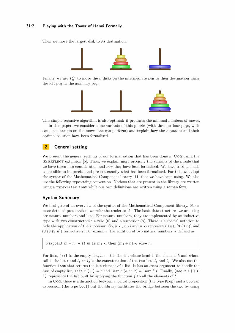
Then we move the largest disk to its destination.

Finally, we use P 3rn to move the n disks on the intermediate peg to their destination using

the left peg as the auxiliary peg.

This simple recursive algorithm is also optimal: it produces the minimal numbers of moves.

In this paper, we consider some variants of this puzzle (with three or four pegs, with

some constraints on the moves one can perform) and explain how these puzzles and their

optimal solution have been formalised.

2 General setting

We present the general settings of our formalisation that has been done in Coq using the

SSReflect extension [5]. Then, we explain more precisely the variants of the puzzle that

we have taken into consideration and how they have been formalised. We have tried as much

as possible to be precise and present exactly what has been formalised. For this, we adopt

the syntax of the Mathematical Component library [11] that we have been using. We also

use the following typesetting convention. Notions that are present in the library are written

using a typewriter font while our own definitions are written using a roman font.

Syntax Summary

We first give of an overview of the syntax of the Mathematical Component library. For a

more detailed presentation, we refer the reader to [5]. The basic data structures we are using

are natural numbers and lists. For natural numbers, they are implemented by an inductive

type with two constructors : a zero (0) and a successor (S). There is a special notation to

hide the application of the successor. So, n.+1, n.+2 and n.+3 represent (S n), (S (S n)) and

(S (S (S n)) respectively. For example, the addition of two natural numbers is defined as

Fixpoint m + n := if m is m1.+1 then (m1 + n).+1 else n.

For lists, [::] is the empty list, h :: t is the list whose head is the element h and whose

tail is the list t and l1 ++ l2 is the concatenation of the two lists l1 and l2. We also use the

function last that returns the last element of a list. It has an extra argument to handle the

case of empty list, last c [::] = c and last c (h :: t) = last h t. Finally, [seq f i | i <-

l ] represents the list built by applying the function f to all the elements of l.

In Coq, there is a distinction between a logical proposition (the type Prop) and a boolean

expression (the type bool) but the library facilitates the bridge between the two by using

L. Thery 31:3

the so-called small scale reflection [7]. As everything is finite in our application, we state

most of our definitions in the boolean world. For example, we use the syntax [rel a b | P]

to define a relation between two arbitrary objects a and b with P being a boolean expression

where the variables a and b can occur. The boolean equality is written a == b, the inequality

a != b. The syntax for boolean operators is !b, b1 && b2, b1 || b2 and b1 ==> b2 for NEG, AND,

OR and IMP respectively. There is a cumulative notation for the AND and the OR : [&& b1, b2,

. . . & bn] and [|| b1, b2, . . . | bn]. Finally, the syntax for the two boolean quantifications

is [forall x : T , P] and [exists x : T , P].

Disks

A disk is represented by its size. We use the type In of natural numbers strictly smaller than

n for this purpose.

Definition disk n := In.

In the following, we use the convention that a variable n will always represent a number of

disks, and d a disk (an element of disk n).

As there is an implicit conversion from In to natural number, the comparison of the

respective size of two disks is simply written as d1 < d2. A minimal element (ord0) and a

maximal element (ord_max) are defined for In when n is not zero2. We use them to represent

the smallest disk and the largest one.

Definition sdisk : disk n.+1 := ord0.

Definition ldisk : disk n.+1 := ord_max.

In particular, ldisk is the main actor of our proofs by simple induction on the number of

disks, it represents the largest disk.

Pegs

We also use In for pegs.

Definition peg k := Ik.

In the following, we use the convention that a variable k will always represent a number of

pegs, and p a peg (an element of peg k).

We mostly use elements of peg 3 or peg 4 but some generic properties hold for peg k. An

operation associated to pegs is the one that picks a peg that differs from an initial peg pi and

a destination peg pj when possible3. It is written as p[pi, pj ]. Generic and specific properties

are derived from it. For example, we have:

2 I0 is an empty type.3 If it is not possible (when working with peg 1 or peg 2), it returns ord0

ITP 2021

31:4 Playing with the Tower of Hanoi Formally

Lemma opeg sym (p1 p2 : peg k) : p[p1, p2] = p[p2, p1].Lemma opegDl (p1 p2 : peg k.+3) : p[p1, p2] != p1.

Lemma opeg3Kl (p1 p2 : peg 3) : p1 != p2 → p[p[p1, p2], p1] = p2.

The symmetry is valid for every number of pegs. The property of being distinct is only

fulfilled when we have more than two pegs. Finally, there is a version of the pigeon-hole

principle for three pegs.

Configuration

If we start from the initial position and follow the rules, all the configurations we can

encounter are such that on each peg, the disks are always ordered from the largest to the

smallest. This means that just recording which disk is on which peg is enough to encode

a configuration. To give an example, if we consider the following configuration with three

disks and three pegs :

knowing that the small disk is on the second peg, the medium disk is on the second peg and

the large disk is on the first peg is enough to recover the information that the small disk is

on top of the medium one.

Configurations are then simply represented by finite functions from disks to pegs.

Definition configuration k n := {ffun disk n → peg k}.

From a technical point of view, using finite functions gives for free functional extensionality

(which is not valid for usual functions in Coq). As a consequence, we can use the boolean

equality == to test equality between two configurations.

A perfect configuration is a configuration where all the disks are on the same peg. So, it

is encoded as the constant function:

Definition perfect p := [ffun d ⇒ p].

It is written as c[p] in the following, or c[p, n] when the number of disks n is given explicitly

in order to help typechecking.

Note that our encoding of configurations has the merit of covering exactly valid config-

urations. The price to pay is that we have to recover some natural notions. One of these

notions is the predicate on top d c that indicates that the disk d is on top of its peg in the

configuration c. It is defined as follows:

Definition on top (d : disk n) (c : configuration k n) :=[forall d1 : disk n, c d == c d1 ==> d ≤ d1].

L. Thery 31:5

It simply states that d is on top if every disk on the same peg as d has a size larger than d.

Most of the main results of the library are proved by some kind of inductive argument.

In order to apply the inductive hypothesis formally, it is then central to be able to see a

subset of a configuration composed of some disks and/or some pegs as a proper configuration

with lesser disks and/or lesser pegs. As configurations are functions, it consists in restricting

the domain and/or the codomain of the function. We call these operations transformations

and usually also define their inverse. Here, we are only going to give an overview of the

transformations we have been using : showing their type and what they are used for but not

their definition. We refer to the library for the actual implementation.

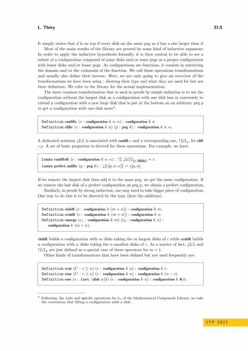
The most common transformation that is used in proofs by simple induction is to see the

configuration without the largest disk as a configuration with one disk less or conversely to

extend a configuration with a new large disk that is put at the bottom on an arbitrary peg p

to get a configuration with one disk more4.

Definition cunliftr (c : configuration k n.+1) : configuration k n.

Definition cliftr (c : configuration k n) (p : peg k) : configuration k n.+1.

A dedicated notation ↓[c] is associated with cunlift c and a corresponding one, ↑[c]p, for clift

c p. A set of basic properties is derived for these operations. For example, we have:

Lemma cunliftrK (c : configuration k n.+1) : ↑[ ↓[c]](c ldisk) = c.

Lemma perfect unliftr (p : peg k) : ↓[c[p, n.+1]] = c[p, n].

If we remove the largest disk then add it to the same peg, we get the same configuration. If

we remove the last disk of a perfect configuration on peg p, we obtain a perfect configuration.

Similarly, in proofs by strong induction, one may need to take bigger piece of configuration.

One way to do this is to be directed by the type (here the addition).

Definition clshift (c : configuration k (m + n)) : configuration k m.

Definition crshift (c : configuration k (m + n)) : configuration k n.

Definition cmerge (c1 : configuration k m) (c2 : configuration k n) :

configuration k (m + n).

clshift builds a configuration with m disks taking the m largest disks of c while crshift builds

a configuration with n disks taking the n smallest disks of c. As a matter of fact, ↓[c] and

↑[c]p are just defined as a special case of these operators for m = 1.Other kinds of transformations that have been defined but not used frequently are:

Definition ccut (C : c ≤ n) (c : configuration k n) : configuration k c.

Definition ctuc (C : c ≤ n) (c : configuration k n) : configuration k (n− c).Definition cset (s : {set (disk n)}) (c : configuration k n) : configuration k #|s|.

4 Following, the lift and unlift operations for In of the Mathematical Component Library, we takethe convention that lifting a configuration adds a disk.

ITP 2021

31:6 Playing with the Tower of Hanoi Formally

Definition cset2 (sp : {set (peg k)}) (sd : {set (disk n)})

(c : configuration k n) : configuration #|sp| #|sd|.

ccut and ctuc are the equivalent of crshift and clshift but directed by the proof C rather than

the type. cset considers a subset of disks but with the same number of peg (#|s| is the cardinalof s). cset2 is the most general and considers both a subset of disks and a subset of pegs.

Move

A move is defined as a relation between configurations. As we want to possibly add constraints

on moves, it is parameterised by a relation r on pegs: r p1 p2 indicates that it is possible

to go from peg p1 to peg p2. Assumptions are usually added on the relation r (such as

irreflexivity or symmetry) in order to prove basic properties of moves.

Here is the formal definition of a move:

Definition move : rel (configuration k n) :=[rel c1 c2 | [exists d1 : disk n,

[&& r (c1 d1) (c2 d1), on top d1 c1, on top d1 c2 &

[forall d2, d1 != d2 ==> c1 d2 == c2 d2]]]].

It simply states that there is a disk d1 that fulfills 4 conditions:

the move of d1 from its peg in c1 to its peg in c2 is compatible with r;

the disk d1 is on top of its peg in c1;

the disk d1 is on top of its peg in in c2;

it is the unique disk that has possibly moved.

The standard puzzle has no restriction on the moves between pegs as long as we don’t

put a large disk on top of a small one. If we draw the possible moves as arrows between pegs,

the picture for four pegs gives the following complete graph:

10 2 3

We call this version regular. It is denoted with the r exponent. For example, P 4r5 corresponds

to the puzzle with four pegs and five disks with no restriction on the moves. Its associated

relation rrel only enforces irreflexivity:

Definition rrel : rel (peg k) := [rel x y | x != y].

Definition rmove : rel (configuration k n) := move rrel.

L. Thery 31:7

The first variant we consider is where one can only move from one peg to its neighbour. The

picture for four pegs is the following:

10 2 3

This version is called linear and its associated infix is l. For example, the puzzle with four

pegs and five disks with linear moves is written P 4l5 . The corresponding relation lrel uses

simple arithmetic to check neighbourhood :

Definition lrel : rel (peg k) := [rel x y | (x.+1 == y) || (y.+1 == x)].

Definition lmove : rel (configuration k n) := move lrel.

Finally the last variant we consider is the one where one central peg is the only one that

can communicate with its outer pegs. A picture for four pegs gives

0

1 2

3

This version is called star and its associated exponent is s. For example, the puzzle with

four pegs and five disks with star moves is written P 4s5 . The corresponding relation srel uses

multiplication to put the peg 0 in the center :

Definition srel : rel (peg k) := [rel x y | (x != y) && (x * y == 0)].Definition smove : rel (configuration k n) := move srel.

Note that these categories may overlap when there are few pegs. For example, P 3ln and P 3s

n

correspond to the same puzzle.

2.1 Path and distance

Moves are defined as relations over configurations. So, we can see sequences of moves as

paths on a graph whose nodes are the configurations. As configurations belong to a finite

type, we can benefit from the elements of graph theory that are present in the Mathematical

Component library. For example, (rgraph move c) returns the set of all the configurations

that are reachable from c in one move, (connect move c1 c2) indicates that c1 and c2 can be

connected through moves, or (path move c cs) gives that the sequence cs of configurations is

a path that connects c with the last element of cs.

Now, all the transformations on configurations need to be lifted to paths. As distinct

configurations may become identical when taking sub-parts, we first need to define an

operation on sequences that removes repetitions.

ITP 2021

31:8 Playing with the Tower of Hanoi Formally

Fixpoint rm rep (A : eqType) (a : A) (s : seq A) :=if n is b :: s1 then

if a == b then rm rep b s1 else b :: rm rep b s1else [::]

It is then possible to derive properties on paths. For example, we have:

Lemma path clshift (c : configuration (m + n)) cs :

path move c cs →path move (clshift c) (rm rep (clshift c) [seq (clshift i) | i <- cs]).

As we want to show that some algorithms are optimal, the last ingredient we need is

a notion of distance between configurations. Unfortunately, there is no built-in notion of

distance in the Mathematical Component library, so we have to define one. For this, we first

build recursively the function connectn that computes the set of elements that are connected

with exactly n moves. Then, we can define the distance between two points x and y as the

smallest n such as (connectn r n x y) holds. It is defined as (gdist r x y) and written as d[x,

y]r in the following. From this definition, the triangle inequality is derived as :

Lemma gdist triangular r x y z : d[x, y]r ≤ d[x, z]r + d[z, y]r.

Finally, we introduce the notion of geodesic path: a path that realises the distance.

Definition gpath r x y p :=[&& path r x p, last x p == y & d[x, y]_r == size p].

Companion theorems are derived for these basic notions. For example, the following lemma

shows that concatenation behaves well with respect to distances.

Lemma gdist cat r x y p1 p2 :

gpath r x y (p1 ++ p2) → d[x, y]_r = d[x, last x p1]_r + d[last x p1, y]_r.

3 Puzzles with three pegs

The proofs associated with the puzzles with three pegs are straightforward. They are done

by induction on the number of disks inspecting the moves of the largest disk. What makes

the simple induction work so well with three pegs is that when, from a configuration c, the

largest disk moves from pi to pj , all the smaller disks in c are necessarily on the peg p[pi, pj ].So, they make a perfect configuration on which one can apply the inductive hypothesis using

↓[c].

3.1 Regular puzzle

It is easy to translate in Coq the algorithm described in the introduction. We write it as a

recursive function that works on n disks and generates the sequence of configurations that

goes from the configuration c[p1] to the configuration c[p2] :

L. Thery 31:9

Fixpoint ppeg n p1 p2 :=

if n is n1.+1 then

let p3 := p[p1, p2] in[seq ↑ [i]p1 | i ← ppeg n1 p1 p3] ++ [seq ↑ [i]p2 | i ← c[p3] :: ppeg n1 p3 p2]

else [::].

We pick an auxiliary peg p3, appropriately lift the results of the two recursive calls and

concatenate them to get the resulting path. It is easy to prove the basic properties of this

function

Lemma size ppeg n p1 p2 : size (ppeg n p1 p2) = 2n − 1Lemma last ppeg n p1 p2 c : last c (ppeg n p1 p2) = c[p2].Lemma path ppeg n p1 p2 : p1 != p2 → path rmove c[p1] (ppeg n p1 p2).

Note that even for such simple theorems, there are some little subtleties. The last ppeg does

hold unconditionally even when the function returns the empty list. It is because this only

happens when the configuration has no disk, so the theorem is an equality between elements

of an empty type. Also, the path ppeg needs the condition p1 != p2 otherwise it will try to

move the largest peg from p1 to p1 that is not valid since the relation rmove is irreflexive.

The key property of the ppeg function is that it builds a path of minimal size. As a

matter of fact, we have proved something slightly stronger : it is the unique minimal path.

In order to state this property, we make use of the extended comparison (e1 ≤ e2 ?= iff C)

that is available in the library. It tells not only that e1 is smaller than e2 but also that the

condition C indicates exactly when the comparison between e1 and e2 is an equality. This

comparison comes with some algebraic rules. For example, the transitivity gives that if (e1≤ e2 ?= iff C1) and (e2 ≤ e3 ?= iff C2) hold, we have (e1 ≤ e3 ?= iff C1 && C2). With

this comparison, the uniqueness and minimality are stated as :

Lemma ppeg min n p1 p2 cs :

p1 != p2 → path rmove c[p1] cs → last c[p1] cs = c[p2] →2n − 1 ≤ size cs ?= iff (cs == ppeg n p1 p2).

The proof is simply done by double induction (one on the size of cs and one on n) inspecting

the moves of the largest disk in the sequence cs. Since p1 differs from p2, we know that

the largest disk must move at least one time in cs. If it moves exactly once, the inductive

hypothesis on n let us conclude directly. If it moves at least twice, the equality never holds.

If the first two moves are on different pegs, adding the inductive hypothesis on n− 1 twice

plus the two moves of the largest disk gives us a path of size at least 2× (2n−1 − 1) + 2 = 2n.

If the largest disk moves on one peg and then returns to the peg p1, the path has some

repetition, so the inductive hypothesis on the size of cs let us conclude.

From this theorem, we easily derive the corollary on the distance.

Lemma gdist rhanoi3p n (p1 p2 : peg 3) :

d[c[p1, n], c[p2, n]]rmove = (2n − 1) × (p1 != p2)

ITP 2021

31:10 Playing with the Tower of Hanoi Formally

Note that we have used the automatic conversion from boolean to integer (true is 1 and

false is 0) to include the case where p1 and p2 are the same peg.

The last theorem only talks about going from a perfect configuration to another one. What

about the distance between two arbitrary configurations c1 and c2? It seems natural to apply

the same greedy strategy always trying to move the largest disk to its destination. The

greedy algorithm would proceed as follows : If c1 ldisk is equal to c2 ldisk, we just perform

the recursive call for smaller disks. If they are different, we perform a recursive call to move

the smaller disks in c1 to an intermediate peg, p[c1 ldisk, c2 ldisk], then move the largest disk

to its position in c2, and finally perform another recursive call to move the smaller disks to

their position in c2. Unfortunately, this natural strategy is not optimal anymore. We can

illustrate this with an example with 3 disks. Let us suppose that we try to go from the initial

configuration:

to the final position:

The greedy strategy would move the largest disk only once and would have size seven, one

for the largest disk, plus two times moving the two small disks. The optimal strategy instead

moves the largest disks twice. It moves it first to the right peg:

and now it follows the greedy strategy and makes four extra moves to reach the target

configuration. So, we have a solution of size five.

We have formalised exactly what the optimal solutions are :

between an arbitrary configuration and a perfect configuration, the greedy strategy is

always optimal;

between two arbitrary configurations c1 and c2, the optimal strategy just needs to compare

the one-jump solution with the two-jump solution only for the largest disk d such that c1d differs from c2 d.

3.2 Linear puzzle

Implementing the greedy strategy for the linear puzzle is slightly more complicated. As we

can move only between pegs that are neighbours, the largest disk may need to jump twice to

reach its destination. But from the optimality point of view the situation is much simpler,

the greedy strategy is always optimal. This is formally proved and we get the expected

theorem about distance between perfect configurations:

Lemma gdist lhanoi3p n (p1 p2 : peg 3) :

d[c[p1, n], c[p2, n]]lmove =if lrel p1 p2 then (3n − 1)/2 else (3n − 1) × (p1 != p2)

L. Thery 31:11

Note that as there are n disks and 3 pegs, there are 3n possible configurations. This last

theorem tells us that the solution that goes from the perfect configuration where all the disks

are on the left peg to the perfect configuration where they are on the right peg visits all the

configurations!

4 Puzzles with four pegs

Adding a peg changes completely the situation. If the previous simple recursive algorithm

still works, it does not give anymore an optimal solution. The new strategy is implemented by

the so-called Frame-Stewart algorithm. We explain it using the regular puzzle with four pegs.

Then, we explain how the proofs about the distances for P 4rn and P 4s

n have been formalised

in Coq.

4.1 The Frame-Stewart Algorithm

Let us build, P 4rn , an algorithm that moves the disks from the leftmost peg to the rightmost

one for the regular puzzles with four pegs.

We choose an arbitrary m smaller than n and use P 4rm to move the top-m disks to an

intermediate peg.

The remaining n−m disks can now freely move except on this intermediate peg, so we can

use P 3rn−m to move them to their destination.

and reuse P4rk to move the top-m disks to their destination.

Now, we can choose the parameter m as to minimise the number of moves. This means that

we have |P 4rn | = min

m<n2|P 4r

m |+ (2n−m − 1). This strategy can be generalised to an arbitrary

ITP 2021

31:12 Playing with the Tower of Hanoi Formally

number k of pegs, leading to the recurrence relation:

|P krn | = min

m<n2|P kr

m |+ |P k−1rn−m |.

Knowing if this general program is optimal is an open question but it has been shown

optimal for P 4rn and P 4s

n . It is what we have formalised. Note that, from the proving point

of view, the new strategy just seems to move from simple induction to strong induction

with this new parameter m. As a matter of fact, if we look closely, this new strategy is just

a generalisation of the previous one. If we apply it to three pegs, taking the minimum is

trivial : there is only one way we can move n−m pegs for the P 2rn−m puzzle; it is by taking

m = n− 1.

4.2 Regular puzzle

The proof given in [2] that shows that the Frame-Stewart algorithm is optimal for the

regular puzzle with four pegs is rather technical. As a matter of fact, this technicality was

a motivation of our formalisation. The proof is very well written and very convincing but

contains several cases which makes it difficult to assess its correctness. A formalisation

ensures that no detail has been overlooked. As an anecdote, the Wikipedia page [13] about

the Tower of Hanoi in March 2020 was indicating that there was actually a journal paper [6]

with a proof of the optimality of the Frame-Stewart algorithm for the regular puzzle with k

pegs. When we started formalising this proof, we quickly got stuck on the formalisation of

Corollary 3. We contacted the author that told us that it was a known flaw in the proof as

documented in [4].

In what follows, we are only going to highlight the overall structure of the proof of

optimality of P 4rn . We refer to the paper proof given in [2] for the details. The first step is to

relate |P 4rn | with triangular numbers. Following [2], we write |P 4r

n | as Φ(n). We introduce

the notation ∆n for the sum of the first n natural numbers :

∆n =∑i≤n

i = n(n + 1)2 .

A number n is triangular if it is a ∆i for some i. By analogy to the square root, we introduce

the triangular root ∇n :

∆(∇n) ≤ n < ∆(∇(n + 1)).

Now, we can give explicit formula for Φ(n) :

Φ(n) =∑i<n

2∆i

It is relatively easy to show that the function Φ verifies the recurrence relation of the Frame-

Stewart algorithm: Φ(n) = minm<n 2Φ(m) + (2n−m − 1). Then, what is left to be proved is

that it is the optimal solution. The key ingredient of the proof is of course to find the right

inductive invariant. This is done thanks to a valuation function Ψ that takes a finite set over

the natural numbers and returns a natural number:

ΨE = maxL∈N

((1− L)2L − 1 +∑n∈E

2min(∇n,L))

The idea is that E will contain the disks we are interested in. If we consider the set [n] of allthe natural numbers smaller than n (i.e. we are interested by all the disks)

[n] = {set i | i < n}

L. Thery 31:13

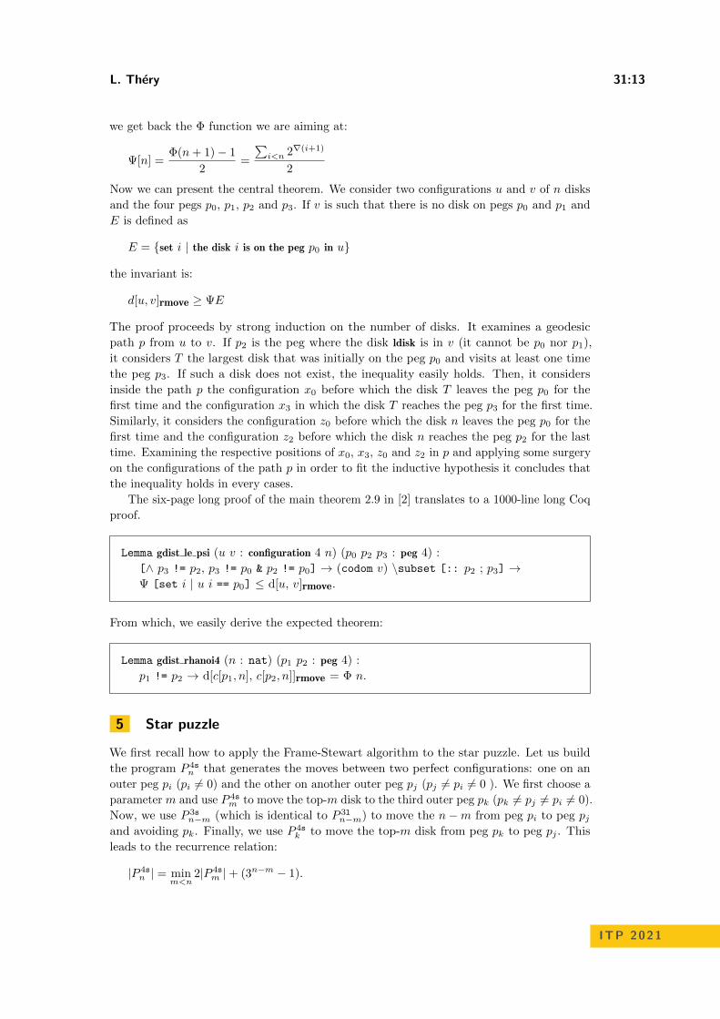
we get back the Φ function we are aiming at:

Ψ[n] = Φ(n + 1)− 12 =

∑i<n 2∇(i+1)

2Now we can present the central theorem. We consider two configurations u and v of n disks

and the four pegs p0, p1, p2 and p3. If v is such that there is no disk on pegs p0 and p1 and

E is defined as

E = {set i | the disk i is on the peg p0 in u}

the invariant is:

d[u, v]rmove ≥ ΨE

The proof proceeds by strong induction on the number of disks. It examines a geodesic

path p from u to v. If p2 is the peg where the disk ldisk is in v (it cannot be p0 nor p1),

it considers T the largest disk that was initially on the peg p0 and visits at least one time

the peg p3. If such a disk does not exist, the inequality easily holds. Then, it considers

inside the path p the configuration x0 before which the disk T leaves the peg p0 for the

first time and the configuration x3 in which the disk T reaches the peg p3 for the first time.

Similarly, it considers the configuration z0 before which the disk n leaves the peg p0 for the

first time and the configuration z2 before which the disk n reaches the peg p2 for the last

time. Examining the respective positions of x0, x3, z0 and z2 in p and applying some surgery

on the configurations of the path p in order to fit the inductive hypothesis it concludes that

the inequality holds in every cases.

The six-page long proof of the main theorem 2.9 in [2] translates to a 1000-line long Coq

proof.

Lemma gdist le psi (u v : configuration 4 n) (p0 p2 p3 : peg 4) :[∧ p3 != p2, p3 != p0 & p2 != p0] → (codom v) \subset [:: p2 ; p3] →Ψ [set i | u i == p0] ≤ d[u, v]rmove.

From which, we easily derive the expected theorem:

Lemma gdist rhanoi4 (n : nat) (p1 p2 : peg 4) :p1 != p2 → d[c[p1, n], c[p2, n]]rmove = Φ n.

5 Star puzzle

We first recall how to apply the Frame-Stewart algorithm to the star puzzle. Let us build

the program P 4sn that generates the moves between two perfect configurations: one on an

outer peg pi (pi = 0) and the other on another outer peg pj (pj = pi = 0 ). We first choose a

parameter m and use P 4sm to move the top-m disk to the third outer peg pk (pk = pj = pi = 0).

Now, we use P 3sn−m (which is identical to P 3l

n−m) to move the n−m from peg pi to peg pj

and avoiding pk. Finally, we use P 4sk to move the top-m disk from peg pk to peg pj . This

leads to the recurrence relation:

|P 4sn | = min

m<n2|P 4s

m |+ (3n−m − 1).

ITP 2021

31:14 Playing with the Tower of Hanoi Formally

Now, we have to find a mathematical object that verifies this recurrence relation. This time

it is not the triangular numbers but the increasing sequence α1 of the elements 2i3j . The

first elements of this sequence are 1, 2, 3, 4, 6, 8, 9. If we define S1(n) =∑

i<n α1(i), it isrelatively easy to prove that

S1(n) = minm<n

2S1(m) + (3n−m − 1)/2.

It follows that 2S1 verifies the recurrence relation.

Here, the proof of optimality is even more intricate, we just give an idea of the inductive

invariant and how the proof proceeds. We refer to [3] for a detailed and very clear exposition of

the proof. The first generalisation is to consider distance not only between two configurations

but between l + 1 configurations (i.e. a distance between u0 and ul passing through u1, . . . ,

ul−1):∑

i<l d[ui, ui+1]. These intermediate configurations (0 < i < l) are alternating. If p1,

p2 and p3 are the outer pegs, the configuration ui is supposed to have its disks on pegs p2and a[p1, p3](i) where alternation is defined as

a[pi, pj ](0) = pi a[pi, pj ](n + 1) = a[pj , pi](n)

Taking into account this new parameter l, we need to lift S1 to a parametrised function Sl.

Sl(n) = minm<n

2S1(m) + l(3n−m − 1)/2

and α1 to αl(n) = Sl(n + 1)−Sl(n). Finally, we introduce the penality function β defined as

βn,l(k) = if 1 < l and k + 1 = n then αl(k) else 2α1(k)

Given these definitions, the inductive invariant looks like:

Lemma main (p1 p2 p3 : peg 4) n l (u : {ffun Il.+1 → configuration 4 n}) :p1 != p2 → p1 != p3 → p2 != p3p1 != p0 → p2 != p0 → p3 != p0 →(∀k, 0 < k < l → codom (u k) subset [:: p2; a[p1, p3] k]) →(S [l] n).*2 ≤ sum (i < l) d[u i, u i.+1] smove +

sum (k < n) (u ord0 k != p1) * β [n, l] k +

sum (k < n) (u ord_max k != a[p1, p3] l) * β [n, l] k.

The proof is done by simple induction on n. It is then split in several cases depending

on the number of elements i such that ui(ldisk) = a[p1, p3](i). Furthermore, the inductive

invariant has this alternating assumption. So, often, one needs to split the path in a bunch of

alternating sub-paths in order to apply the inductive hypothesis on each of these sub-paths.

This leads to a lower-bound where various values of Si(m) appear. Key properties of Sl(n)(i.e. its convexity5 in n and concavity6 in l) are then used to derive simpler lower-bounds.

For example, the combination of these two theorems

5 A function on natural numbers is convex if f and n 7→ f(n + 1) − f(n) are both increasing.6 A function on natural numbers is concave if f is increasing and n 7→ f(n + 1) − f(n) is decreasing.

L. Thery 31:15

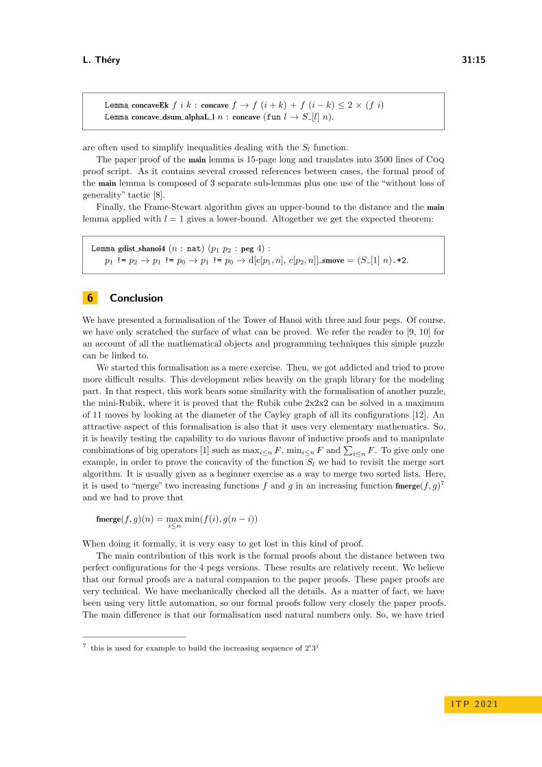
Lemma concaveEk f i k : concave f → f (i + k) + f (i− k) ≤ 2 × (f i)Lemma concave dsum alphaL l n : concave (fun l → S [l] n).

are often used to simplify inequalities dealing with the Sl function.

The paper proof of the main lemma is 15-page long and translates into 3500 lines of Coq

proof script. As it contains several crossed references between cases, the formal proof of

the main lemma is composed of 3 separate sub-lemmas plus one use of the “without loss of

generality” tactic [8].

Finally, the Frame-Stewart algorithm gives an upper-bound to the distance and the main

lemma applied with l = 1 gives a lower-bound. Altogether we get the expected theorem:

Lemma gdist shanoi4 (n : nat) (p1 p2 : peg 4) :p1 != p2 → p1 != p0 → p1 != p0 → d[c[p1, n], c[p2, n]] smove = (S [1] n).*2.

6 Conclusion

We have presented a formalisation of the Tower of Hanoi with three and four pegs. Of course,

we have only scratched the surface of what can be proved. We refer the reader to [9, 10] for

an account of all the mathematical objects and programming techniques this simple puzzle

can be linked to.

We started this formalisation as a mere exercise. Then, we got addicted and tried to prove

more difficult results. This development relies heavily on the graph library for the modeling

part. In that respect, this work bears some similarity with the formalisation of another puzzle,

the mini-Rubik, where it is proved that the Rubik cube 2x2x2 can be solved in a maximum

of 11 moves by looking at the diameter of the Cayley graph of all its configurations [12]. An

attractive aspect of this formalisation is also that it uses very elementary mathematics. So,

it is heavily testing the capability to do various flavour of inductive proofs and to manipulate

combinations of big operators [1] such as maxi≤n F , mini≤n F and∑

i≤n F . To give only one

example, in order to prove the concavity of the function Sl we had to revisit the merge sort

algorithm. It is usually given as a beginner exercise as a way to merge two sorted lists. Here,

it is used to “merge” two increasing functions f and g in an increasing function fmerge(f, g)7and we had to prove that

fmerge(f, g)(n) = maxi≤n

min(f(i), g(n− i))

When doing it formally, it is very easy to get lost in this kind of proof.

The main contribution of this work is the formal proofs about the distance between two

perfect configurations for the 4 pegs versions. These results are relatively recent. We believe

that our formal proofs are a natural companion to the paper proofs. These paper proofs are

very technical. We have mechanically checked all the details. As a matter of fact, we have

been using very little automation, so our formal proofs follow very closely the paper proofs.

The main difference is that our formalisation used natural numbers only. So, we have tried

7 this is used for example to build the increasing sequence of 2i3j

ITP 2021

31:16 Playing with the Tower of Hanoi Formally

to avoid as much as possible subtraction. In our formal setting, (m− n) + n = m is a valid

theorem only if we add the assumption that n ≤ m. So an expression such as a− b ≤ c− d

in the paper proof is translated into a + d ≤ b + c in the formal development.

Our formal proofs can, of course, be largely improved. To cite only one example, in

the proof of the star puzzle with 4 pegs, lots of subcases are proved by simple symbolic

manipulations with applications of some concavity theorems like concaveEk. These are

currently done by hand. There is clearly room for automating all these steps.

References

1 Yves Bertot, Georges Gonthier, Sidi Ould Biha, and Ioana Pas,ca. Canonical Big Operators.

In TPHOLs, volume 5170 of LNCS, Montreal, Canada, 2008.

2 Thierry Bousch. La quatrieme tour de Hanoı. Bull. Belg. Math. Soc. Simon Stevin, 21(5):895–

912, 2014.

3 Thierry Bousch. La Tour de Stockmeyer. Seminaire Lotharingien de Combinatoire, 77(B77d),

2017.

4 Thierry Bousch, Andreas M. Hinz, Sandi Klavzar, Daniele Parisse, Ciril Petr, and Paul K.

Stockmeyer. A note on the Frame-Stewart conjecture. Discrete Math., Alg. and Appl., 11(4),

2019.

5 Mathematical Component. The SSReflect Proof Language. Section of the Coq refence manual,

available at https://coq.inria.fr/refman/proof-engine/ssreflect-proof-language.

html.

6 Roberto Demontis. What is the least number of moves needed to solve the k-peg Towers of

Hanoi problem? Discrete Math., Alg. and Appl., 11(1), 2019.

7 Georges Gonthier, Assia Mahboubi, and Enrico Tassi. A Small Scale Reflection Extension

for the Coq system. Research Report RR-6455, Inria, 2016. URL: https://hal.inria.fr/

inria-00258384.

8 John Harrison. Without loss of generality. In TPHOLs 2009, volume 5674 of LNCS, pages

43–59, 2009.

9 Andreas M. Hinz, Sandi Klavzar, Uros Milutinovic, and Ciril Petr. The Tower of Hanoi –

Myths and Maths. Birkhauser, 2013.

10 Ralf Hinze. Functional pearl: la tour d’Hanoı. In ICFP, pages 3–10. ACM, 2009.

11 Assia Mahboubi and Enrico Tassi. Mathematical components. available at https://math-comp.

github.io/mcb/book.pdf.

12 Laurent Thery. Proof Pearl: Revisiting the Mini-Rubik in Coq. In TPHOLs, volume 5170 of

LNCS, pages 310–319. Springer, 2008.

13 Wikipedia. Tower of Hanoi, March 2020. available at https://en.wikipedia.org/w/index.

php?title=Tower_of_Hanoi&oldid=943067350.