Proof and Computation in Geometry

Michael Beeson

San Jose State University, San Jose, CA

Abstract. We consider the relationships between algebra, geometry,computation, and proof. Computers have been used to verify geomet-rical facts by reducing them to algebraic computations. But this doesnot produce computer-checkable first-order proofs in geometry. We mighttry to produce such proofs directly, or we might try to develop a “back-translation” from algebra to geometry, following Descartes but with com-puter in hand. This paper discusses the relations between the two ap-proaches, the attempts that have been made, and the obstacles remain-ing. On the theoretical side we give a new first-order theory of “vectorgeometry”, suitable for formalizing geometry and algebra and the rela-tions between them. On the practical side we report on some experimentsin automated deduction in these areas.

1 Introduction

The following diagram should commute:

Geometric Proof Algebraic Proof

Geometric Theorem Algebraic Translation

That diagram corresponds to the title of this paper, in the sense that proofis on the left side, computation on the right. The computations are related togeometry by the two interpretations at the top and bottom of the diagram. Inthe past, much work has been expended on each of the four sides of the diagram,both in the era of computer programs and in the preceding centuries. Yet, we stilldo not have machine-found or even machine-checkable geometric proofs of thetheorems in Euclid Book I, from a suitable set of first-order axioms–let alone themore complicated theorems that have been verified by computerized algebraiccomputations.1 In other words, we are doing better on the right side of thediagram than we are on the left.

1 A very good piece of work towards formalizing Euclid is [1], but because it mixescomputations (decision procedures) with first-order proofs, it does not furnish acounterexample to the statement in the text.

2

First-order geometrical proofs are beautiful in their own right, and they givemore information than algebraic computations, which only tell us that a result istrue, but not why it is true (i.e. what axioms are needed and how it follows fromthose axioms). Moreover there are some geometrical theorems that cannot betreated algebraically at all (because their algebraic form involves inequalities).

We will discuss the possible approaches to getting first-order geometricalproofs, the obstacles to those approaches, and some recent efforts. In particularwe discuss efforts to use a theorem-prover or proof-checker to facilitate a “backtranslation” from algebra to geometry (along the bottom of the diagram). Thispossibility has existed since Descartes defined multiplication and square rootgeometrically, but has yet to be exploited in the computer age. According toChou et. al. ([8], pp. 59–60), “no single theorem has been proved in this way.”

To accomplish that ultimate goal, we must first bootstrap down the left sideof the diagram as far as the definitions of multiplication and square root, as thatis needed to interpret the algebraic operations geometrically. We will discussthe progress of an attempt to do that, using the axiom system of Tarski andresolution theorem-proving.

1.1 That commutative diagram, in practice

In theory, there is no difference between theory and practice.In practice, there is.

– Yogi Berra

Here is a version of the diagram, with the names of some pioneers2 , andon the right the names of the computational techniques used in the algebraiccomputations arising from geometry. The dragon, as in maps of old, representsuncharted and possibly dangerous territory.

Here be dragons

Geometric Proof Algebraic “Proof”

Geometric Theorem Algebraic Translation

Grobner bases

CAD (Collins)

Chou’s area method

Wu-Ritt method

Narboux

Szmielew

Tarski

Euclid

Chou, Wu, Descartes

Descartes, Hilbert

2 Many others have contributed to this subject, including Gelernter, Gupta, Kapur,Ko, Kutzler and Stifter, and Schwabhauser.

3

Our proposal is the following:

(i) The goal is the lower left, i.e. first-order geometric proofs.

(ii) Finding them directly is difficult (hence the dragon in the picture).

(iii) Therefore: let’s get around the dragons by going across the bottom fromright to left.

1.2 Issues raised by this approach

The first issue is the selection of a language and axioms (that is, a theory) inwhich to represent geometrical theorems and find proofs. We discuss that brieflyin the next section, and settle upon Tarski’s language and the axioms for ruler-and-compass geometry.

The next issue is this: if we want to go around the right side of the diagramand back across the bottom, and end up with a proof, then the computationalpart (the algebra on the right side of the diagram) will have to be formalized insome theory. In other words, we will have to convert computations to verified,or formal computations (proofs in some algebraic theory).3 A formal theory ofalgebra will be required.

The third issue is, how can we connect the left and right sides of the diagram?If we have a formal geometrical theory on the left, and a formal algebraic theoryon the right, we need (at the least) two formal translation algorithms, one ineach direction. Technically such mappings (taking formulas to formulas) arecalled “interpretations”; we will need them to take proofs to proofs as well asformulas to formulas.

That approach promises to be cumbersome: two different formal theories, twoformal interpretations, algebraic computations, and proofs verifying the correct-ness of those computations. We will cut through some of these complications byexhibiting a new formal theory VG of “vector geometry.” This theory suffices toformalize the entire commutative diagram, i.e. both algebra and geometry. Thefirst half of this paper is devoted to the formal theories for geometry, algebra,and vector geometry, and some metatheorems about those theories.

Within that theoretical framework, there is room for a great deal of practicalexperimentation. We have carried out some preliminary experiments, on whichwe report. In these experiments, we used the resolution-based theorem proversOtter and Prover9, but that is an arbitrary choice; one could produce proofsby hand using Coq as in [20]4 or in another proof-checker, or using anothertheorem-prover.

3 This is related to the general problem of verifying algebraic computations carriedout by computer algebra systems, which often introduce extra assumptions thatoccasionally result in incorrect results.

4 There is an issue about how easy it is or is not to extract first-order geometric proofsfrom a Coq proof. In my opinion it should be possible, but Coq proofs are not prima

facie first-order.

4

2 First order theories of geometry

In this section we discuss the axiomatization of geometry, and its formalizationin first-order logic. These are not quite the same thing, as there is a long his-tory of second order axiomatizations (involving sets of points). Axiomatizationshave been given by Veblen [33], Pieri [24], Hilbert [14], Tarski [31], Borsuk andSzmielew [5], and Szmielew [29], and that list is by no means comprehensive.

The following issues arise in the axiomatization of geometry:

– What are the primitive sorts of the theory?– What are the primitive relations?– What (if any) are the function symbols?– What are the continuity axioms?– How is congruence of angles defined?– How is the SAS principle built into the axioms?– How close are the axioms to Euclid?– Are the axioms few and elegant, or numerous and powerful?– Are the axioms strictly first-order?– Can the axioms be stated in terms of the primitives, or do they involve

defined concepts?– Do the axioms have a simple logical form (e.g. universal or ∀∃)?

Evidently there is no space to discuss even the few axiomatizations mentionedabove with respect to each of these issues; we point out that the answers to thesequestions are more or less independent, which gives us at least n = 211 differentways to formalize geometry, whose relationships and mutual interpretations canbe studied. Nearly every possible combination of answers to the “issues” hassomething to recommend it. For example, Hilbert has several sorts, and his ax-ioms are not strictly first-order; Tarski has only one sort (points) and ten axioms.My own theory of constructive geometry [4, 3] has points, lines, and circles, andfunction symbols so that the axioms are quantifier-free and disjunction-free.

In Euclid, geometry involves lines, line segments, circles, arcs, rays, angles,and “figures” (polygons). Rays and segments are needed only for visual effect,so a formal theory can dispense with them.

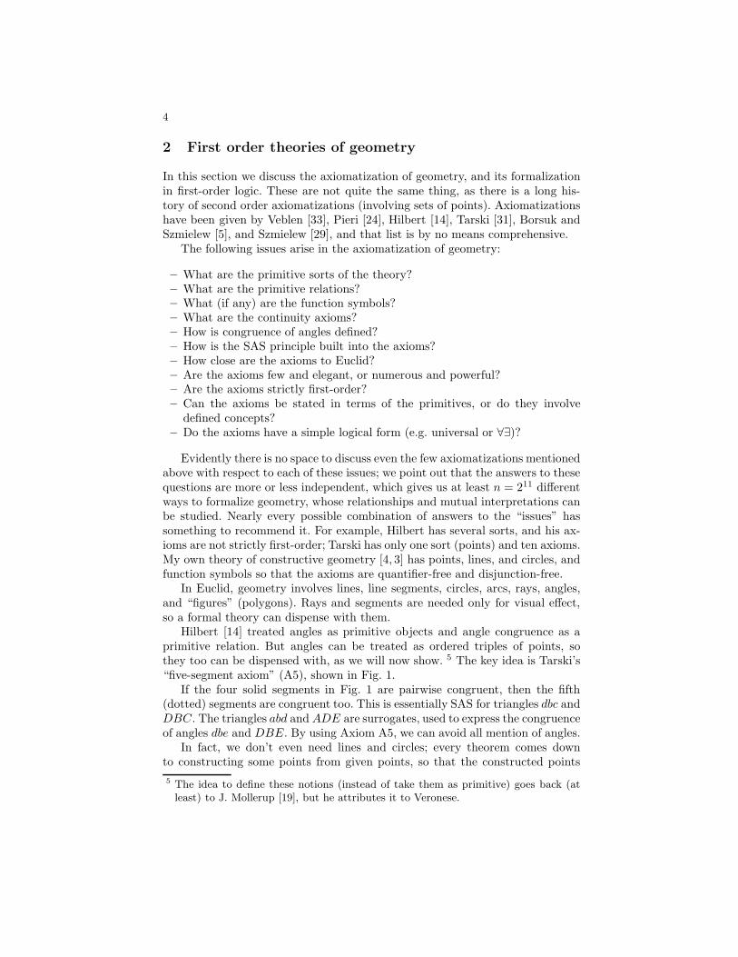
Hilbert [14] treated angles as primitive objects and angle congruence as aprimitive relation. But angles can be treated as ordered triples of points, sothey too can be dispensed with, as we will now show. 5 The key idea is Tarski’s“five-segment axiom” (A5), shown in Fig. 1.

If the four solid segments in Fig. 1 are pairwise congruent, then the fifth(dotted) segments are congruent too. This is essentially SAS for triangles dbc andDBC. The triangles abd and ADE are surrogates, used to express the congruenceof angles dbe and DBE. By using Axiom A5, we can avoid all mention of angles.

In fact, we don’t even need lines and circles; every theorem comes downto constructing some points from given points, so that the constructed points

5 The idea to define these notions (instead of take them as primitive) goes back (atleast) to J. Mollerup [19], but he attributes it to Veronese.

5

Fig. 1. The five-segment axiom (A5)

d

a b c

D

A B C

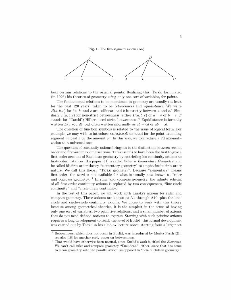
bear certain relations to the original points. Realizing this, Tarski formulated(in 1926) his theories of geometry using only one sort of variables, for points.

The fundamental relations to be mentioned in geometry are usually (at leastfor the past 120 years) taken to be betweenness and equidistance. We writeB(a, b, c) for “a, b, and c are collinear, and b is strictly between a and c.” Sim-ilarly T (a, b, c) for non-strict betweenness: either B(a, b, c) or a = b or b = c. Tstands for “Tarski”; Hilbert used strict betweenness.6 Equidistance is formallywritten E(a, b, c, d), but often written informally as ab ≡ cd or ab = cd.

The question of function symbols is related to the issue of logical form. Forexample, we may wish to introduce ext(a,b,c,d) to stand for the point extendingsegment ab past b by the amount cd. In this way, we can reduce a ∀∃ axiomati-zation to a universal one.

The question of continuity axioms brings us to the distinction between secondorder and first-order axiomatizations. Tarski seems to have been the first to give afirst-order account of Euclidean geometry by restricting his continuity schema tofirst-order instances. His paper [31] is called What is Elementary Geometry, andhe called his first-order theory “elementary geometry” to emphasize its first-ordernature. We call this theory “Tarksi geometry”. Because “elementary” meansfirst-order, the word is not available for what is usually now known as “rulerand compass geometry.”7 In ruler and compass geometry, the infinite schemaof all first-order continuity axioms is replaced by two consequences, “line-circlecontinuity” and “circle-circle continuity.”

In the rest of this paper, we will work with Tarski’s axioms for ruler andcompass geometry. These axioms are known as A1 through A10, plus the line-circle and circle-circle continuity axioms. We chose to work with this theorybecause among geometrical theories, it is the simplest in the sense of havingonly one sort of variables, two primitive relations, and a small number of axiomsthat do not need defined notions to express. Starting with such pristine axiomsrequires a long development to reach the level of Euclid; this formal developmentwas carried out by Tarski in his 1956-57 lecture notes, starting from a larger set

6 Betweenness, which does not occur in Euclid, was introduced by Moritz Pasch [21];see also [16] for another early paper on betweenness.

7 That would have otherwise been natural, since Euclid’s work is titled the Elements.We can’t call ruler and compass geometry “Euclidean”, either, since that has cometo mean geometry with the parallel axiom, as opposed to “non-Euclidean geometry.”

6

of axioms; and then by 1965 the axioms were reduced to A1-A10 plus continuity.For a history of this development see [32] or the foreword to [29].

3 Fields and Geometries

In this section we briefly review the known results connecting formal theories ofgeometry with corresponding formal theories of algebra (field theory).

A Euclidean field is an ordered field in which every positive element has asquare root; or equivalently (without mentioning the ordering), a field in whichevery element is a square or minus a square, every element of the form 1 + x2 isa square, and -1 is not a square.

If F is a Euclidean field, then using analytic geometry we can expand F2 toa model of ruler and compass geometry.

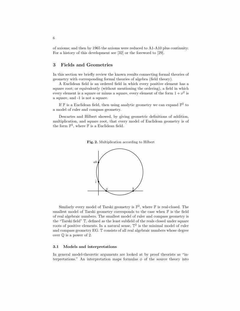
Descartes and Hilbert showed, by giving geometric definitions of addition,multiplication, and square root, that every model of Euclidean geometry is ofthe form F2, where F is a Euclidean field.

Fig. 2. Multiplication according to Hilbert

bab

bi

ba

bb

Similarly every model of Tarski geometry is F2, where F is real-closed. Thesmallest model of Tarski geometry corresponds to the case when F is the fieldof real algebraic numbers. The smallest model of ruler and compass geometry isthe “Tarski field” T, defined as the least subfield of the reals closed under squareroots of positive elements. In a natural sense, T2 is the minimal model of rulerand compass geometry EG. T consists of all real algebraic numbers whose degreeover Q is a power of 2.

3.1 Models and interpretations

In general model-theoretic arguments are looked at by proof theorists as “in-terpretations.” An interpretation maps formulas φ of the source theory into

7

formulas φ of the target theory, preserving provability:

⊢ φ ⇒ ⊢ φ

Usually the proof also shows how to transform the proofs efficiently. Generallyinterpretations have several advantages over models, all stemming from theirgreater explicitness. The main advantage is that an interpretation enables oneto translate proofs from one theory to another. A model theoretic theorem,coupled with the completeness theorem, may imply the existence of a proof,but not give the slightest clue how to find it; while interpretations often give alinear-time proof translation.

There is a price to be paid, as the technical details of interpretations are oftenmore intimidating than those of the corresponding model-theoretic arguments.Nevertheless, if we hope to use the equivalences of geometry and algebra to findproofs, model theory will not suffice. We need explicit interpretations.

Another reason for working with interpretations is that they can also be usedfor theories with non-classical logics, for example intuitionistic logic. The detailsof the interpretations between geometry and field theory can be found in [3].Below, after introducing a theory of vector geometry, we will give a sample ofthese details.

3.2 Interpretations between geometry and algebra

Here we sketch the main ideas connecting formal theories of geometry and al-gebra, indicating how these ideas can be expressed using interpretations ratherthan model theory. Since at this point we have not given an explicit list of ax-ioms, the discussion cannot be completely precise, but still the ideas can beexplained. When we go from algebra to geometry, we fix a line L, which wecall the “x-axis”, containing two fixed distinct points α and β. (These interpretthe scalars 0 and 1.) Then we show that one can construct a line perpendicularto any given line K, passing through a given point q, without needing a casedistinction as to whether q is or is not on K. Since we do not have variables forlines, we need two points (say k1 and k2) to specify K and two to specify theresulting line, so we need two terms perp1(k1, k2, q) and perp2(k1, k2, q) that de-termine this perpendicular. Then we define “the y-axis” to be the perpendicularto the x-axis at α. We can then define coordinate functions X and Y by terms ofour geometrical theory, such that for any point q, X(q) is a point P on the fixedline L such that the line containing X(q) and q is perpendicular to L, and theline containing q perpendicular to the y-axis meets the y-axis at a point Q suchthat Qα ≡ αY (q). (Notice that Q is on the y-axis but Y (q) is on the x-axis.)It is not at all trivial to construct these terms without a test-for-equality func-tion (symbol), but it can be done (see [3]).8 Then we can find a term F of our

8 This permits us to eschew a test-for-equality symbol, which is good, for two reasons:nothing like a test-for-equality construction occurs in Euclid, and simpler is better.But [3] uses terms for the intersections of lines and circles; whether those can beeliminated is not known.

8

geometrical theory that takes two points x and y on the x-axis and constructsthe point p whose coordinates are x and y. One first constructs the point Q onthe y-axis such that αQ ≡ αy, and the the lines perpendicular to the x axis atx and perpendicular to the y axis at Q. One needs the parallel postulate (A10)to prove that these lines actually meet in the desired point F (x, y).

Part of the price to pay for using interpretations instead of models is thatthe algebraic interpretation φ⋆ of a geometric formula φ has two free variablesfor each free variable of φ, one for each coordinate. Then when we translate backinto geometry, these two variables do not recombine, but become two differentpoint variables, restricted to the x-axis. They must be recombined using F .

3.3 Euclid lies in the AE fragment

By the AE fragment, or the ∀∃ fragment, we mean the set of formulas of theform ∀x∃y A(x, y), where x and y may stand for zero or more variables, and Ais quantifier-free.

Euclid’s theorems have the form,

Given some points bearing certain relations to each other, there exist(one can construct) certain other points bearing specified relations to theoriginal points and to each other.

The case where no additional points are constructed is allowed. The points areto be constructed with ruler and compass, by constructing a series of auxiliarypoints. Constructed points are built up from the intersections of lines and circles.

Theorems of this form can be translated into Euclidean field theory (formu-lated with a function symbol for square root). Since the intersections of lines andcircles, and the intersections of circles, can be expressed using only quadraticequations, and there is a function symbol for square root, constructed pointscorrespond to terms of the theory. Euclid’s theorems are thus in ∀∃ form, bothbefore and after translation into algebra.

A careful analysis of Euclid’s proofs shows that, apart from some case dis-tinctions as to whether two points are equal or not, or a point lies on a line ornot, the proofs are constructive: Euclid provides a finite number of terms, one ofwhich works in each case. This is closely related to Herbrand’s theorem, whichwould tell us that if ∀x∃y A(x, y) is provable, then there are finitely many termst1, . . . , tn such that the disjunction of the A(x, ti(x)) is provable.

Some parts of Euclid are about “figures”, which are essentially arbitrarypolygons. Euclid did not have the language to express these theorems precisely,since that would require variables for finite sets or lists or points, but we regardthem as “theorem schemata”, i.e. for each fixed number of vertices, we have aEuclidean theorem.

The AE fragment of the modern first-order theory of ruler and compassgeometry is thus the closest thing we have to a formal analysis of Euclid. Eucliddid not study theorems with more alternations of quantifiers.

9

3.4 Decidability issues

A proper study of the relations between proof and computation in geometrymust take place against the backdrop of the many known, and a few unknown,results about the decidability or undecidability of various theories. After all,the decidability of a formal theory means that provability in the theory can bereduced to computation. We offer in this section a summary of these known andunknown results.

Godel and Church showed that in number theory, provability cannot be re-duced to computation; Tarski showed that in geometry, it can, in the sense thatTarski geometry can be reduced to the theory RCF of real closed fields, for whichTarksi gave a decision procedure. Later Fischer and Rabin [10] showed that anydecision procedure for RCF is at least exponential in the length of the input,and others showed it is at least double exponential in the number of variables;and Collins gave a decision procedure that is no worse than that bound (Tarski’swas). (See [27] for more details.) Thus from a practical point of view it doesn’tdo us any good to know that RCF is decidable. There are interesting questionsthat can be formulated in RCF, questions whose answers we do not know, butif they involve more than six variables, then we are not going to compute theanswers by a decision procedure for RCF.

On the other hand, if we drop the continuity axioms entirely, we get back thecomplications of number theory. Julia Robinson [28] proved that Q is an unde-cidable field, and later extended this result to algebraic number fields. Regardingthe decidability of theories rather than particular fields, Ziegler [36] proved thatany finitely axiomatizable extension of field theory is undecidable–in particularthe theory of Euclidean fields. His proof shows the AEA fragment is undecid-able. (Here AEA means ∀∃∀, formulas with three blocks of unlike quantifiers asindicated.) It does not say anything about the AE fragment. It is presently anopen problem whether the AE fragment of RCF (and hence the AE fragment ofTarski geometry) is decidable. The fact that Euclid’s Elements lies within thisfragment focuses attention on the problem of its decidability.

Tarski conjectured that T (recall that T2 is the smallest model of rule andcompass geometry) is undecidable, but this is still an open problem. Since T isnot of finite degree over the rationals, its undecidability is not implied by JuliaRobinson’s results about algebraic number fields.

4 Tarski’s ruler and compass geometry

In this section we comment on the axioms of Tarski’s theory, which can befound in full formal detail in [32] or [29]. This section is intended both as anintroduction to Tarski’s axioms, and as a description of the Skolem symbols weadded to make the theory quantifier-free instead of ∀∃. As mentioned above, theprimitives are non-strict betweenness T and segment congruence ab ≡ cd, whichis a 4-ary relation between points.

10

4.1 Tarski’s first six axioms

Axiom A5 has been discussed and illustrated above. The other five are

uv ≡ vu (A1)

uv ≡ wx ∧ uv ≡ yz → wx ≡ yz (A2)

uv ≡ ww → u = v (A3)

T (u, v, ext(u, v, w, x)) (A4), segment extension

T (u, v, u) → u = v (A6)

We have added a Skolem symbol to express (A4) without a quantifier.

4.2 Pasch’s axiom (1882)

Moritz Pasch [21] (See also [22], with an historical appendix by Max Dehn)supplied an axiom that repaired many of the defects that nineteenth-centuryrigor found in Euclid. Roughly, a line that enters a triangle must exit thattriangle. As Pasch formulated it, it is not in AE form. There are two AE versions,illustrated in Fig. 4.2. These formulations of Pasch’s axiom go back to Veblen[33], who proved outer Pasch implies inner Pasch. Tarski took outer Pasch as anaxiom in [31].

Fig. 3. Inner Pasch (left) and Outer Pasch (right). Line pb meets triangle acq in oneside. The open circles show the points asserted to exist on the other side.

b

a x

bq

bc

bb

bp

b

ab

qx

bb

b c

b

p

Tarski originally took outer Pasch as an axiom, but following the “final”version of Tarski’s theory in [29], we take inner Pasch. Seeking a quantifier-freeformulation, we introduce a function symbol ip to produce the intersection pointsfrom the five points labeled in the diagram. When the betweenness relations inthe diagram are not satisfied, nothing is asserted about the value of ip on thosepoints.

11

4.3 Gupta’s thesis

In his 1965 thesis [12] under Tarski, H. N. Gupta proved two great theorems:9

(i) Inner Pasch implies outer Pasch. After that Szmielew’s development usedinner Pasch as an axiom (A7) and dropped outer Pasch (although Tarski wasstill arguing decades later [32] for the other choice).

(ii) Connectivity of Betweenness:

a 6= b ∧ T (a, b, c) ∧ T (a, b, d) → T (a, c, d) ∨ T (a, d, c).

That is, betweenness determines a linear order of points on a line. Points d andc, both to the right of b on Line(a, b), must be comparable.

The connectivity of betweenness was taken as an axiom by Tarski, but onceGupta proved it dependent, it could be dropped. Gupta never published histhesis, but his proof of connectivity appears as Satz 5.1 in [29]. The proof iscomplicated: it uses 8 auxiliary points and more than 70 inferences, and uses allthe axioms A1-A7. His proof of outer Pasch (from inner Pasch) also occurs in[29] as Satz 9.6.

4.4 Dimension Axioms

(A8) (lower dimension axiom) says there are three non collinear points (noneof them is between the other two)

(A9) (upper dimension axiom) says that any three points equidistant fromtwo distinct points must be collinear. In other words, the locus of points equidis-tant from a and b is a line (not a plane as it would be in R3).

(A1) through (A9) are the axioms for “Hilbert planes.”

4.5 Tarski’s Parallel Axiom (A10)

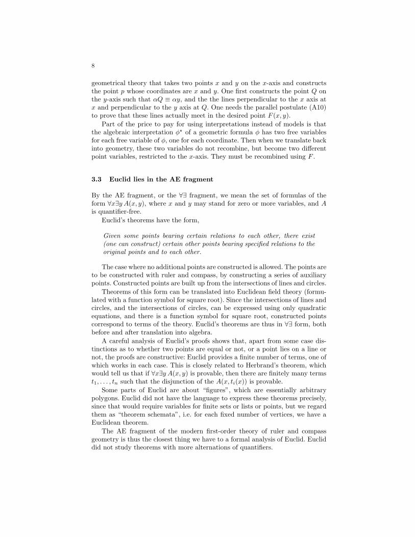
In the diagram (Fig. 4), open circles indicate points asserted to exist. There areother equivalent forms; see [32, 29].10 We would need to introduce new functionsymbols to work with A10 in a theorem-prover. Since none of the work in thispaper depends on the exact formulation of the parallel axiom, we do not discussalternate formulations.

4.6 Line-circle continuity

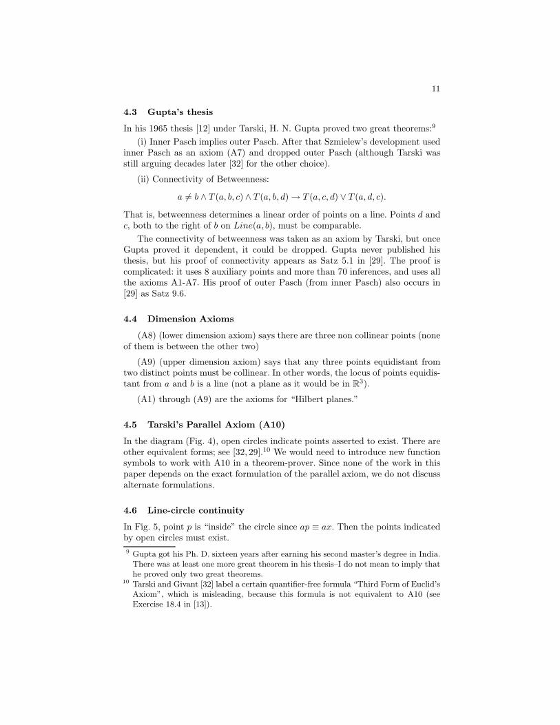
In Fig. 5, point p is “inside” the circle since ap ≡ ax. Then the points indicatedby open circles must exist.

9 Gupta got his Ph. D. sixteen years after earning his second master’s degree in India.There was at least one more great theorem in his thesis–I do not mean to imply thathe proved only two great theorems.

10 Tarski and Givant [32] label a certain quantifier-free formula “Third Form of Euclid’sAxiom”, which is misleading, because this formula is not equivalent to A10 (seeExercise 18.4 in [13]).

12

Fig. 4. Tarski’s parallel axiom

x y

ba

bb

bc

bt

bd

Fig. 5. Line-circle continuity. Line L is given by two points A, B (not shown). Thepoints shown by open circles are asserted to exist.

ba

L

bb b

x

b

p

We use two function symbols ℓc1 and ℓc2 to name the points ℓc1(A,B, a, x, b, p)and ℓc2(A,B, a, x, b, p), where A and B are two unequal points that determinethe line L. In [3], we also introduce another axiom, the point of which is toensure that the two intersection points occur in the same order on L as A andB. This can be expressed as a disjunction of several betweenness statements,essentially listing the possible allowed orders of the four points. Since non-strictbetweenness is used in this axiom, the points p and x might be on the circle, inwhich case the line is tangent to the circle and the two intersection points coin-cide. The additional axiom implies that the two intersection points each dependcontinuously on their arguments. Tarski used an existential quantifier instead offunction symbols to formulate line-circle continuity, so the extra axiom was notneeded; but we want a quantifier-free axiomatization, and the extra axiom isnatural so that there will be one natural model F2 over each Euclidean field F,instead of uncountably many with strange discontinuous interpretations of ℓc1and ℓc2.

13

4.7 Circle-circle continuity

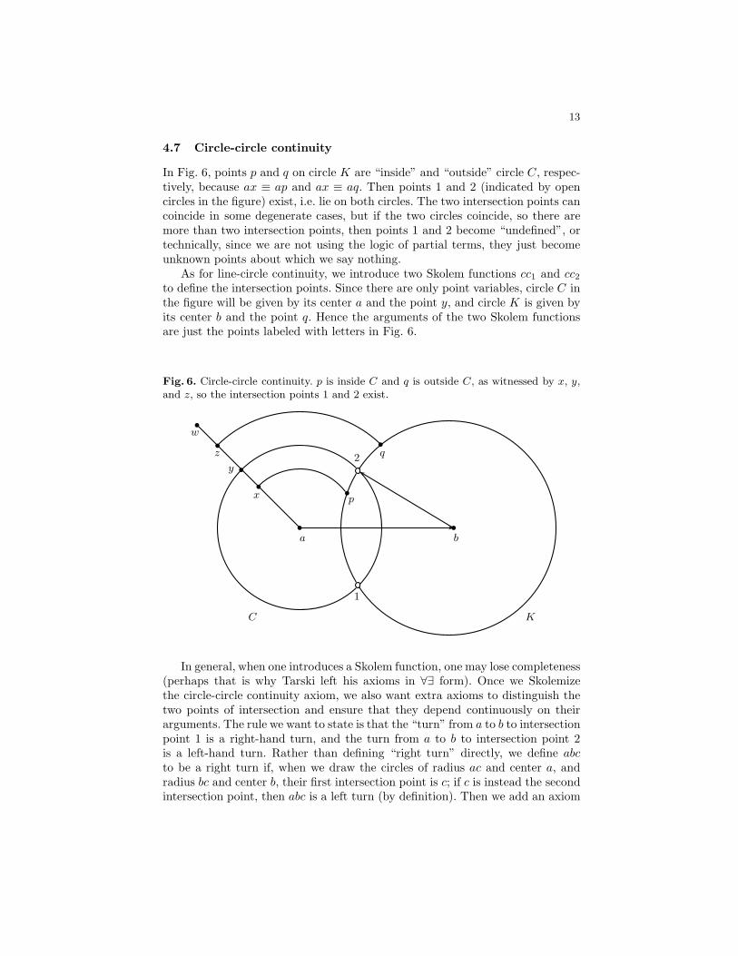
In Fig. 6, points p and q on circle K are “inside” and “outside” circle C, respec-tively, because ax ≡ ap and ax ≡ aq. Then points 1 and 2 (indicated by opencircles in the figure) exist, i.e. lie on both circles. The two intersection points cancoincide in some degenerate cases, but if the two circles coincide, so there aremore than two intersection points, then points 1 and 2 become “undefined”, ortechnically, since we are not using the logic of partial terms, they just becomeunknown points about which we say nothing.

As for line-circle continuity, we introduce two Skolem functions cc1 and cc2to define the intersection points. Since there are only point variables, circle C inthe figure will be given by its center a and the point y, and circle K is given byits center b and the point q. Hence the arguments of the two Skolem functionsare just the points labeled with letters in Fig. 6.

Fig. 6. Circle-circle continuity. p is inside C and q is outside C, as witnessed by x, y,and z, so the intersection points 1 and 2 exist.

b

b

b

a

b

z

b

w

by

b

x

b

q

b

p

2

1

KC

In general, when one introduces a Skolem function, one may lose completeness(perhaps that is why Tarski left his axioms in ∀∃ form). Once we Skolemizethe circle-circle continuity axiom, we also want extra axioms to distinguish thetwo points of intersection and ensure that they depend continuously on theirarguments. The rule we want to state is that the “turn” from a to b to intersectionpoint 1 is a right-hand turn, and the turn from a to b to intersection point 2is a left-hand turn. Rather than defining “right turn” directly, we define abcto be a right turn if, when we draw the circles of radius ac and center a, andradius bc and center b, their first intersection point is c; if c is instead the secondintersection point, then abc is a left turn (by definition). Then we add an axiom

14

saying that if c and d are on the same side of the line through a and b, and abcis a right turn, so is abd, and the same for left turns. For the definition of “sameside”, we follow [29], Definition 9.7, p. 71. Since these axioms play no role in thispaper, we refer the interested reader to [3] for further details.

5 VG, a formal theory of vector geometry

In this section, we describe a first-order theory VG that contains both geometryand algebra. This theory permits us to formalize the relationships between al-gebra and geometry in both directions, and to formalize the Chou area methoddirectly. The theories of algebra and of geometry become fragments of VG.

5.1 Language of Vector Geometry

Three sorts:

– points p, q, a, b– scalars α, β, λ, s, t– vectors u, v

Intuitively you may think of vectors as equivalence classes of directed line seg-ments under the equivalence relation of parallel transport. Constructors andaccessors:

– p ◦ q is a vector, the equivalence class of directed segment pq.– scalar multiplication: λu is a vector– dot product: u · v is a scalar– cross product: u× v is a scalar (not a vector, we are in two dimensions)

5.2 Language of Vector Geometry

Relations:

– betweenness and equidistance from Tarski’s language– Equality for points, equality for vectors, equality for scalars. Technically

these are different symbols.– x < y for scalars.

Function symbols (other than constructors and accessors) and constants:

– Skolem symbols for Tarski’s language, specifically ext for segment exten-sion, ip for inner Pasch, and Skolem symbols for line-circle and circle-circlecontinuity, as described above.

– 0, 1, ∗,+, /, unary and binary −, and√

for scalars.– 0 is a vector; u + v, u− v, and −u are vectors.– 0, 1, and i are unequal points.– i is a point equidistant from 1 and from −1 = ext(1, 0, 0, 1).

15

5.3 Division by zero and square roots of negative numbers

1/0 is “some scalar” rather than “undefined”, because we want to use theoremprovers with this language and they do not use the logic of partial terms. Onecannot prove anything about 1/0 so it does not matter that it has some unde-termined value. For example, we have the axiom x 6= 0 → x ∗ (1/x) = 1, not theaxiom x ∗ (1/x) = 1. Other “undefined” terms are treated the same way.

5.4 Axioms of Vector Geometry VG

– Tarski’s axioms for ruler-and-compass geometry.– The scalars form a Euclidean field.– The obvious axioms for unary − and / and

√permit us to avoid existen-

tial quantifiers in the axioms for Euclidean fields. The use of binary − is aconvenience; the axiom is a− b = a+ (−b).

– The vectors form a vector space over the scalars.– The usual laws for dot product and 2d cross product.– a ◦ b = −b ◦ a– p ◦ p = 0– E(0, i, 0, 1)– E(i, 1, i,−1) where −1 = ext(1, 0, 1, 0)– If ab and cd are parallel and congruent, then a ◦ b = ±c ◦ d, with the sign

positive if segment ad meets segment bc, and negative if it does not.– If a, b, c, and d are collinear and ab and cd are congruent, then a◦b = ±c◦d,

with the appropriate sign (given by betweenness conditions expressing theintuitive idea that the sign is positive if the directed segments ab and cd havethe same direction).

The geometrical part (based on Tarski’s axioms A1-A10 and line-circle andcircle-circle continuity, but in a quantifier-free form) we call “Euclidean geome-try” EG. There are function symbols for the intersection points of two lines, of aline and a circle, and of two circles; that is a slightly different choice of functionsymbols from the quantifier-free version of Tarski’s axioms used in this paper.See [3] for a detailed formulation.

5.5 Analytic geometry in VG

This corresponds to the translations across the top and bottom of our (suppos-edly) commutative diagram. Let φ be a formula of EG. Let φ⋆ be a translationof φ into Euclidean field theory (expressed using scalar variables in VG). In fact,more generally we can define φ⋆ when φ is a formula of VG, not just of EG.

The first thing to notice here is that there is more than one way to definesuch a translation φ. The obvious one is the one that is taught to middle-schoolchildren, which we call the “Cartesian translation.” Lines are given by linearequations, and points by pairs of numbers. In practice this leads to many casedistinctions as vertical lines require special treatment. Another translation, in-vented by Chou [8], takes a detour through vectors, but can be expressed directly

16

in VG, and then (whichever way we interpreted points), of course vectors canbe expressed by coordinates using the scalars of VG. We will discuss the Choutranslation in more detail below. The important fact, expressing the adequacyof VG for this part of the method, is the following theorem.

Theorem 1 (Analytic Geometry). Let φ be a formula of VG. Let φ⋆ beeither the Cartesian translation of φ, or the Chou translation. Then

VG ⊢ φ implies EF ⊢ φ⋆

where EF is the theory of Euclidean fields.

Remark. This corresponds to the top of the commutative diagram.

Proof. Here we discuss only the Cartesian translation. By “the x-axis” we meanthe line containing α and β, where α and β are the two distinct points mentionedin the dimension axioms. Next we define the Cartesian interpretation φ⋆ of φ.To define φ⋆, we have to first assign a term t⋆, or a pair of terms (t1, t2), of EFfor each term t of EG. In fact, we define t⋆ for all terms of VG, not just EG.Since points and vectors are to be interpreted as pairs of scalars, we use pairsfor terms of those types; for a term of EF we just have t⋆ = t. Otherwise wewrite t⋆ = (t⋆1, t

⋆

2). When t is a point variable x, then x occurs in the official listof all point variables as the n-th entry, for some n, and we define x⋆ to be thepair consisting of the scalar variables occurring with indices 4n and 4n+1 in theofficial list of scalar variables. Similarly for vector variables, but using indices4n+ 2 and 4n+ 3.

The definitions of φ⋆ for the case of atomic formulas involving betweennessor segment congruence is straightforward analytic geometry. For details see [13]or [3]. To extend the definition of φ⋆ from EG to VG, we have to show that dotproduct and cross product of vectors can be algebraically defined. For example,

(t× s)⋆ = (t⋆1s⋆

2 − t⋆2s⋆

1)

Once t⋆ is defined, then φ⋆ commutes with the logical connectives and quanti-fiers, except that for quantifiers, each point or vector variable is “doubled”, i.e.changed to two scalar variables.

Now the theorem is proved by induction on the length of proofs in VG. Thebase case is when φ is an axiom of VG. We verify in EF that the algebraicallydefined relations of betweenness and equidistance satisfy the axioms of EG. Thatis lengthy, and not entirely straightforward, in the case of circle-circle continuity(but note that the same complications occur whether we are using model theoryor interpretations). See, for example, [13], page 144. See also [3] for some detailsomitted in [13]. We note that if φ is quantifier-free (or AE) in EG, then φ⋆ isalso quantifier-free (or AE).

5.6 Geometric arithmetic in VG

Along the bottom of the commutative diagram, we have a translation φ◦ fromEF to EG, following Descartes with improvements by Hilbert. We show that

17

this translation can be extended to be defined on terms and formulas of VG, notonly of EF. We fix a particular line L (given by the two unequal points α and β,which we use as the interpretations of 0 and 1, respectively). Scalars of VG areinterpreted as points on L, i.e. collinear with α and β. Vectors are interpretedas pairs of such points. Since there is no pairing function in EG, the formula φ◦

may have more variables than φ, as each vector variable converts to two pointvariables. The terms (t+s)◦, (t−s)◦, (−t)◦, (t ·s)◦, and (

√t)◦, are defined using

terms of EG. For example, the definition of (t · s)◦ should be the one suggestedby Fig. 2.

It is not at all obvious that t◦ can be defined using the terms of EG, which donot include a symbol for definition-by-cases; in other words there are no termsin EF to construct a term d(a, b) that is equal to α if a = b and to β otherwise.But the definitions of addition and multiplication given by Descartes requiresuch a case distinction; Hilbert’s multiplication does not, but his addition stilldoes. We have shown in [3] that an improved (continuous) definition of additioncan be given; there only constructive logic is used, but here that is not an issue.If that were not true, we would simply include a definition-by-cases symbol inEG, and our main results would not be affected; but it is not necessary. Forcomplete details of the interpretation from EF to EG, see [3].

Theorem 2 (Geometric algebra). Let φ be a formula of EG. Let φ◦ be thetranslation discussed above of VG into EG. Then

VG ⊢ φ implies EG ⊢ φ◦

VG ⊢ φ implies EG ⊢ (φ⋆)◦

Remark. This corresponds to the bottom of the commutative diagram.

Proof sketch. It has to be verified geometrically that multiplication, addition, andsquare root satisfy the laws of Euclidean field theory. This goes back to Descartesand Hilbert, but as noted above, since we do not have a test-for-equality functionin EG, a more careful definition of addition is required. Since we have extendedthe interpretation to VG, we also need to verify the laws of vector spaces andof cross product and dot product geometrically. It is possible to do this directly,but we can also circumvent the need for those details, by defining φ◦ to be (φ⋆)◦

for formulas φ involving vectors. Note that the language of VG has no termsconstructing vectors from points, so if φ contains terms of type vector, it doesnot contain betweenness or equidistance or any subterms of type point. Henceit is not actually necessary to directly verify the laws of cross product and dotproduct and vector spaces geometrically.

5.7 Conservativity and commutativity

Suppose we start with a geometric theorem φ and somehow prove either it or φ⋆

with the aid of analytic geometry. (By Theorem 1, if we have a proof of φ⋆, wecan get a proof of φ, and vice-versa.) Then can we eliminate the “scaffolding” ofanalytic geometry, and find a purely geometric proof of φ? Yes, we can:

18

Theorem 3. VG is a conservative extension of EG. That is, if φ is a formulain the language of Tarski’s geometry EG, and VG proves φ, then EG proves φ.

Proof. Suppose φ is a formula of EG, and VG proves φ. Then by Theorem 2,φ◦ is provable in EG. But φ◦ is φ since φ is a formula of EG. That completesthe proof of the theorem.

Suppose we start with a formula φ of Euclidean field theory, and find a proofof it using vectors, or even using the full apparatus of VG. Then it is alreadyprovable from the axioms of Euclidean fields:

Theorem 4. VG is a conservative extension of Euclidean field theory EF.

Proof. Suppose φ is a formula of Euclidean field theory EF, and suppose VGproves φ. Then φ⋆ is provable in EF. But by definition of φ⋆, when φ is a formulaof EF, φ⋆ is exactly φ. Hence EF proves φ. That completes the proof.

Next we show that the two interpretations φ⋆ and ψ◦ are, up to provableequivalences, inverses. This is by no means immediate, since the definitions haveno apparent relation to one another. But nevertheless, they both express thesame geometric relationships.

Theorem 5 (Commutativity). Let φ be a formula of EG with no free vari-ables. Then

(φ⋆)◦ ↔ φ

is provable in EG. Similarly, if ψ is a theorem of EF with no free variables,then

(ψ◦)⋆ ↔ ψ

is provable in EF.

We will not give a proof of this theorem here, as it is highly technical. Thetheorem has to be first formulated in a way that holds for formulas with freevariables, as well as for formulas without, and then proved by induction on thecomplexity of φ. The technical issue here is the “doubling” of variables when wepass from point variables to scalar variables, and the “uncoordinatizing” in theother direction. We will explain what “uncoordinatizing” means next.

We will illustrate the proof by explaining one example, the case when φis T (α, y, β). Then the point variable y is “doubled” by φ⋆ to the two scalarvariables (λ1, λ2), intuitively representing the coordinates of y. (Defining thisprecisely depends on setting up a one-to-two correspondence between the listsof variables of type point and type scalar.) Then φ⋆ is

λ2 = 0 ∧ 0 ≤ λ1 ∧ λ1 ≤ 1.

Now going back to geometry, the two scalar variables do not convert back toone point variable. Instead they become two variables of type point, y1 and y2,restricted (by (φ⋆)◦) to lie on the x-axis (the line through α and β). We writeCol(x, y, z) for “x, y, and z lie on the line containing distinct points x and y”,

19

defined in terms of betweenness. Then (φ⋆)◦ is equivalent to (though not literallythe same as)

Col(α, β, y1) ∧ Col(α, β, y2) ∧ y2 = α ∧ T (α, y1, β).

Finally we construct the point q = F (y1, y2) using the F described above. ThenX(q) = y1 and Y (q) = y2. Then

(φ(y)⋆)◦ ↔ ((φ⋆)(λ1, λ2))◦

↔ φ(q)

(φ(y)⋆)◦ ↔ φ(F (y1, y2)) (1)

Here y1 and y2 are point variables related to the original point variable y by thisrule: if y is the n-th point variable xn, then y1 is x2n and y2 is x2n+1. Now thevariables on the left side of (1) are not related to the variables on the right inany semantic way; to state the commutativity theorem for φ we need this:

y = F (y1, y2) → ((φ(y)⋆)◦ ↔ φ(y)) (2)

where in spite of appearances the formula ((φ(y)⋆)◦ contains y1 and y2 free,not y. Equation (2) demonstrates the way that φ ↔ (φ⋆)◦ is generalized toformulas with free variables. Granted, this is technical, but it works and is insome sense natural, and it is the price we have to pay for the benefits of anexplicit interpretation. Once this is correctly formulated, the rest of the proof isstraightforward (which is not the same thing as “short”).

5.8 Algebra in VG

When we “prove” a geometric theorem by making a corresponding algebraiccomputation, we have not yet proved anything; we have only made a computa-tion. In order to convert such a computation (ultimately) to a geometric proof,it will first be necessary to convert an algebraic computation to an algebraicproof. This also goes under the name of “verifying a computation”, or some-times, “verifying the correctness of a computation.”

What we want to prove is that “computationally equal” terms t and s areprovably equal. For example, we can compute by simple algebra that

(x2 − y2)2 + 4x2y2 = (x2 + y2)2

But that does not deliver into our hands a formal proof of that equation fromthe axioms of Euclidean field theory.

The principal problem here is that “computationally equal” is not very welldefined. One is at first tempted to say: if your favorite computer algebra systemsays the terms are equal, they are computationally equivalent. But if we takethat definition, then it is false that computationally equivalent terms are provablyequal. For example, Sage and Mathematica agree that x · (1/x) = 1, but that is

20

not provable in EF, since, if it were, we would have 0 ·1/0 = 1, but since 0 ·z = 0we also have 0 · 1/0 = 0, hence 1 = 0, but 1 6= 0 is an axiom of EF.

Such problems arise from the axioms of EF that are not equational, forexample x 6= 0 → x · (1/x) = 1 and x ≥ 0 → (

√x)2 = x. If we use these

equations without regard to the preconditions, false results can be obtained.We do not know how to define “computationally equivalent terms” except by

provability of t = s in EF, or more generally, the vector and scalar part of VG.The search for a theorem or general result degenerates to a practical problem:given a computation by a computer algebra system that t = s, determine theminimal “side conditions” φ on the variables of t = s necessary for the provabilityof t = s and find a first-order proof of t = s. One may or may not wish to considerparamodulation steps as legal.

5.9 Chou’s method formalizable in VG

This subsection presumes familiarity with Chou’s method [8]. Readers withoutthat prerequisite may skip this subsection and continue reading, but since Chou’smethod is an important method of proving geometrical theorems by algebraiccomputations, we want to verify that it can be directly formalized in VG.

We start with Chou’s basic concept, the position ratio. In VG, we define

ab

cd:= pr(a, b, c, d) =

(a ◦ b) · (c ◦ d)(c ◦ d) · (c ◦ d)

Our pr is defined whenever c 6= d. Chou’s position ratio is defined only when a,b, c, and d are collinear, but in that case they agree.

Chou makes extensive use of the signed area of an oriented triangle. We definethat concept in VG by

A(p, q, r) :=1

2(q ◦ p) × (q ◦ r).

Chou’s other important concepts and theorems can also be defined and provedin VG. In particular, the co-side theorem can be proved in VG. This should bechecked by machine; it would make a good master’s thesis.

6 Finding formal proofs from Tarski’s Axioms

An essential part of the project of making our diagram commute is to find formalproofs in geometry up to the point where multiplication, addition, and squareroot can be geometrically defined and their field-theoretic properties proved. Wechose to attack this project using Tarski’s axioms and resolution theorem provers.One of the reasons for this choice is the existence of a very detailed “semiformal”development due to Szmielew.11 Another reason is that others have tried in the

11 Wanda Szmielew developed course notes for her course in the Foundations of Geom-etry at UC Berkeley, 1965-66, and gave a copy to her successor as instructor of thatcourse, Wolfram Schwabhauser. These notes incorporated important contributionsfrom Gupta’s thesis [12], including the two theorems mentioned above. After herdeath, her notes were published with “inessential changes” as part of [29].

21

past to work with resolution theorem provers and Tarski’s axioms. Specifically,MacPharen, Overbeek, and Wos [18] worked 37 years ago with Tarski’s 1959system; after the publication of [29], Quaife [25, 26] used Otter to formalize thefirst four of the fifteen chapters of Szmielew’s development (that is, Chapters 2-5out of 2-16). Quaife solved some, but not all, of the challenge problems from [18],and added some challenge problems of his own. In 2006, Narboux [20] checkedSzmielew’s proofs using Coq, up through Chapter 12. While this is fine work, thefact remains that after almost forty years, we have collectively still not producedcomputer-checked proofs of Szmielew’s development–whether by an automatedreasoning program (such as Otter), an interactive proof-checker (such as Coq),or by any other means.12

Wos and I undertook to make another attempt. One aim of this projectis to produce a formal proof of each theorem (“Satz”) in Szmielew, using ashypotheses (some of) the previous theorems and definitions, with the ultimateaim of formalizing the definitions and properties of multiplication, addition, andsquare root.

A second aim of the project is to see how much the techniques available forautomated deduction have improved in the 20 years since Quaife. Would we nowbe able to solve the challenge problems that were left unsolved at that time?

And ultimately, a third aim of the project is to reach the propositions ofEuclid, but based on Tarski’s axioms.

6.1 Szmielew in Otter

Larry Wos and I experimented with going through Szmielew’s development,making each theorem into an Otter file, giving Otter the previously proved the-orems to use. We also used Prover9 sometimes, but we found it did not performnoticeably better (or worse) on these problems. Our aim was to obtain Otterproofs of each of Szmielew’s theorems.

Some basic facts about Otter (and Prover9) will be helpful. Otter gives aweight to every formula (by default, the total number of symbols). You canartificially adjust the weights using a list called the “weight list”. There is aparameter called max weight; formulas with larger weights are discarded to keepthe search space down. Thus you can control the search to some degree byassigning certain formulas low weights and finding a good value of max weight

that allows a proof to be found: just large enough that all needed formulas arekept, not so large that the prover drowns in irrelevant conclusions. These remarksapply to both Otter and Prover9; the difference between the two provers lies inthe algorithm for choosing the next clauses to be considered for generating newclauses.

One technique we used is called “giving Otter the diagram.” This meansdefining a name for each of the points that need to be constructed. For example,

12 William Richter has also checked Szmielew up through Satz 3.1 in miz3(see http://www.math.northwestern.edu/˜richter/TarskiAxiomGeometry.ml). Hehas also checked some proofs from Hilbert’s axioms; the code is inhol light/RichterHilbertAxiomGeometry/ in the HOL-Light distribution.

22

if the diagram involves extending segment ab beyond b by an amount cd, youwould add the line q = ext(a, b, c, d). The point of doing so is that q, being anatom, gets weight 1, so terms involving q will be more likely to be used, and lesslikely to be discarded.

We also used “hints” and “resonators” [34]. By this we mean the following:

(i) We put some of the proof steps (from the book proof) in as preliminarygoals. We get proofs of some of them.

(ii) We put the steps of those proofs into Otter’s weight list, giving them alow weight, to ensure that they be chosen quickly to make new deductions. Thebound max weight is then set to the smallest value that will ensure their reten-tion. This prevents the program from drowning in new and possibly irrelevantconclusions.

The technique of resonators can be used in other ways as well. For example,if you are trying to prove C and you have proofs of some lemma A and a proofof C from the assumption A, but you cannot directly get a proof of C, then putthe steps of the two proofs you do have in as resonators. Very likely you will findthe desired proof of C. Wos has also used resonators very successfully to findshorter proofs, once a long proof is in hand.

6.2 What happened

Our first observation was that it is necessary to give Otter the diagram, in thesense described above. Once we started doing that, we went through Chapters2 and 3 (of 2–16) rapidly and without difficulty.

We hit our first snag at Satz 4.2. An argument by cases according as a = cor a 6= c is used. Otter could do each case, but not the whole theorem! We triedProver9. Prover 9 could prove Satz 4.2, but it took 67,000 seconds! (1 day =86,400 sec.)

The inability to argue by cases is a well-known problem in resolution theorem-proving. On perhaps ten (out of more than 100) subsequent theorems, we hadto help Otter with arguments by cases. Sometimes we did that by putting in thecase split explicitly, and giving the cases low weights. For example we would putin b=c | b!=c and then give both literals a negative weight. With this trick,if the cases can be done in separate runs, we could sometimes get a proof in asingle run.13 If not, then we used the proof steps of both cases as resonators.

Chapter 5 of [29] contains a difficult theorem from Gupta’s thesis [12], theconnectivity of betweenness (Satz 5.1). That theorem is

a 6= b ∧ T (a, b, c) ∧ T (a, b, d) → T (a, c, d) ∨ T (a, d, c).

13 Ross Overbeek suggested a general strategy: if you don’t get a proof, look for thefirst unit ground clause deduced, and argue by cases (in two runs) on that clause.That strategy would have worked on Satz 4.2. Here is a project: implement thisstrategy using parallel programming.

23

Neither Otter nor Prover9 could prove Gupta’s theorem without help. We usedresonators, starting with about thirty of Gupta’s proof steps. This technique wassuccessful. We found a proof of Satz 5.1.

After proving the connectivity of betweenness, we had no serious difficultieswith the rest of Chapters 5 and 6; Otter required no help except a couple of casesplits.

In 1990, Quaife made a pioneering effort (using Otter) to find proofs inTarski’s geometry. He used the version of Tarski’s axioms [29], just as we do.Quaife made it a bit farther than where Wos and I hit our first snag in Szmielew.Most of Quaife’s theorems are in Szmielew Chapters 2 and 3, or the first partof 4, or are similar to such theorems, but use some defined notions such as“reflection,” which occurs in Chapter 7 of [29]. His most difficult example wasthat the diagonals of a “rectangle” bisect each other. Here a “rectangle” is aquadrilateral with two opposite sides equal and the diagonals equal. This theoremis weaker than Lemma 7.21 in [29], which says that in a quadrilateral in which(both pairs of) opposite sides are congruent, the diagonals bisect each other.

Quaife left four challenge problems, which are theorems in that part of [29]that we formalized. Although he did not say so explicitly, it is clear that theseshould be solved from axioms A1-A9, i.e. without the parallel axiom or anycontinuity assumptions. We list them here:

– the connectivity of betweenness (Satz 5.1 in [29])– every segment has a midpoint (Satz 8.22 in [29]).– inner Pasch implies outer Pasch (Satz 9.6 in [29])– Construct an isosceles triangle with a given base (an immediate corollary of

Satz 8.21 and Satz 8.22, the existence of midpoints and perpendiculars).

The difficulty of proving the existence of a midpoint lies in the fact thatno continuity axioms are allowed. (The usual construction using two circles isthus not applicable.) This requires developing the theory of right angles andperpendiculars, and takes most of Chapters 7 and 8 of [29]. The constructiondepends on two difficult theorems: the construction of a perpendicular to a linefrom a point not on the line, and the construction of a perpendicular to a linethrough a point on the line (Satz 8.18 and 8.20). These in turn depend on anothertheorem of Gupta, called the “Krippenlemma” (Lemma 7.22). The proof thatinner Pasch implies outer Pasch is one of the highlights of [12].

6.3 Our results

We were eventually able to prove all four of Quaife’s challenge problems, andindeed all the results from [29] up to and including Satz 9.6. The proofs we found,the Otter input files to produce them, and some discussion of our techniques, areavailable at [2]. Satz 7.22 (the Krippenlemma) and Satz 8.18 (construction of theperpendicular) were extremely difficult, and required many iterations of proofs ofintermediate results, and incorporation of new resonators from those proofs. Wecould never have found these Otter proofs without the aid of Gupta’s proofs,

24

so in some sense this is “computer-assisted deduction”, intermediate between“proof-checking” and “automated deduction.”

Why were we able to do better in 2012 than Quaife could do in 1990? Wasit that we used faster computers with larger memories? No, it was that weused techniques unknown to Quaife. We could not find these proofs with 2012computers using only Quaife’s techniques. Maybe we could have found the proofswe found with 1990 computers and 2012 techniques, but we’re glad we didn’thave to. Quaife knew how to tell Otter what point to construct (and we learnedthe technique from him), but he didn’t know about resonators.

6.4 Euclid from Tarski

As of summer 2012, neither by hand nor by machine had development fromTarski’s axioms reached the first proposition of Euclid, more than half a centuryafter Tarski formulated his axioms, although an approach from a far less parsi-monious axiom set has allowed the mechanization of some of Euclid [1]. Quaifedid not get as far as proving any theorem about circles. Neither did Szmielewor Gupta. All these authors wanted to postpone the use of even line-circle orcircle-circle continuity as long as possible, while Euclid uses it (implicitly) fromthe outset. We felt that it was high time to prove at least the first propositionof Euclid from Tarski’s axioms.

Euclid’s Book I, Prop. 1. constructs an equilateral triangle, as shown in Fig. 7.The open circle indicates the constructed point. Euclid’s proof does not meetthe modern standards of rigor, according to which one would need some sort ofcontinuity axiom and perhaps some sort of dimension axiom to prove Prop. 1,since if the circles were in different planes, they would not meet. It turns outthat the dimension axioms are not needed, because “circle-circle continuity” issphere-sphere continuity in R3.

Fig. 7. Euclid Book I, Proposition 1

b bA B

25

The result: Otter proves Euclid I.1 from circle-circle continuity in less thantwo seconds, with a good choice of inference rules. When we first did it, it tookeleven minutes, which is about how long it will take you by hand.

Euclid’s Prop I.2 says that given three points A, B, and C, a point D can beconstructed such that AD = BC. That is immediate from Tarski’s segment ex-tension axiom (A4). Euclid only postulated you can extend a segment somehow,so in a sense, Tarski’s (A4) is unnecessarily strong.

Euclid’s Prop I.3 mentions the concepts “the greater” and “the lesser” be-tween segments. In Tarski’s primitives, we would define ab ≤ cd to mean thatfor some x we have ab ≡ cx and T (c, x, d). Then Prop. I.3 has no content; inother words Prop. I.3 amounts to a definition of “the greater” and “the lesser”,which in Euclid are “common notions.”

Prop. I.4 is the SAS congruence criterion. That requires defining angle con-gruence; it is Satz 11.4 in Szmielew! There is a big jump from the first threepropositions to Prop. I.4. The reason is that angle congruence and indeed com-parison of angles (≤ for angles) are primitive in Euclid, but defined in Tarski’ssystem. The resulting complications have little to do with automated deduction.They are the consequence of choosing a very parsimonious formal language.Therefore, we should complete Szmielew Chapter 11 first, or take some axiomsabout comparison and congruence of angles, in order to formalize Euclid directly.(That is the approach taken in [1].) We plan to return to Euclid after finishingthe formalization of Szmielew up to Chapter 11. For example, Euclid’s Prop. I.8is the SSS angle criterion, Satz 11.51 in Szmielew.

7 Proof by computation, in theory and practice

In this section, we discuss the top and right sides of the diagram. The plan,in theory, is to verify the truth of (which in a loose sense is to prove), somegeometric formula A. We start by expressing it as a system of algebraic equations(or inequalities) using analytic geometry (or by some other method), introducingnew variables for the coordinates of the points to be constructed (or some otherquantities depending on those points). Then we calculate to see if these equationscan be satisfied. If the calculation succeeds, then A is verified. But we still donot have a first-order proof of A.

To put this method into practice, we need to answer two questions: Exactlyhow will we convert from geometry to algebra, and exactly how will we makethe required computations? Among the ways to convert geometry to algebra, wemention the ordinary introduction of coordinates, and Wu’s method [35], andChou’s area method [8]. Among the ways to compute, we mention Grobner basesand the Collins CAD algorithm [7, 6]. While theoretically, any geometry problemcan be solved by CAD, since it is a decision procedure for real-closed fields, inpractice, it breaks down on problems with five or six (number) variables, soa geometry problem with four points is likely to be intractable, and geometryproblems with fewer than four points are rare. On the other hand, Wu’s methodand Chou’s area method have been used to prove hundreds of beautiful theorems,

26

some of them completely new. In that sense, they far outperformed resolutiontheorem proving.

In spite of the dramatic successes of these methods, we point out two short-comings. First, both these methods work only on theorems that translate toalgebra using equations, with no inequalities. Thus the “simple” betweennesstheorems of Szmielew Chapter 3 are out-of-scope.

Second, you cannot ask for a proof from ruler-and-compass axioms (or indeedfrom any geometric axioms at all). You can only ask if the theorem is true inR2. Thus there is no problem trisecting an angle; this is not about ruler-and-compass geometry. A proposition like Euclid I.1 is just trivial: all the subtletiesand beauties of the first-order proof are not captured by these methods. It justcomputes algebraically that there is a point on both circles.

In short, when using these methods, we are not doing geometry. We are doingalgebra. It is these shortcomings that we propose might be rectified, if we couldmake the diagram commute in practice. Then we could go along the bottom ofthe diagram, benefiting from computation on the right, and still end up withgeometrical proofs on the left.

In theory, we should be able to get geometric proofs by going across thebottom of the diagram from right to left. That is, to convert the algebra per-formed by Chou’s method into first-order proofs of algebraic theorems, fromsome algebraic axioms, and then back-translate to geometry, using the geomet-ric definitions of addition and multiplication. In theory this can certainly bedone. In practice, the authors of [8] were aware of this possibility, and discussit on pp. 59–60, but they say, “The geometric proofs produced in this way areexpected to be very long and cumbersome, and as far as we know no single the-orem has been proved in this way.” Nevertheless, those proofs, if we could findthem, would be proofs and not just computations.

8 From computation to proof: going around the dragons

Here is the plan to find a first-order proof of a given geometric theorem by goingacross the top of the diagram, down the right, and back, all within VG.

– Start with a geometric theorem φ to be proved.– Do the analytic geometry to compute φ⋆. (By Chou or Descartes)– Find (e.g. by Chou’s program or by hand) an informal proof that φ⋆ is true,

by calculation.– Get a formal proof in VG of φ⋆, i.e., verify the calculation.– Use (an implementation of) Theorem 1 to get a proof of φ in VG.– Eliminate the non-geometrical axioms to get a proof of φ. This can be done,

at least in theory, by (an implementation of) Theorem 3.

The main point to be made about this plan is that the difficulty is essentiallya “boot-strapping” issue. To get started, we need (machine) formalization of thegeometric definitions of addition, multiplication, and square root. These proofs

27

need to be produced just once, and then we can use them to find proofs of manydifferent geometrical theorems. The central importance of the theorems justify-ing these definitions has long been recognized, as these theorems are in somesense the culminating results of both [14] and [29]. Indeed, the key to provingthe properties of multiplication (no matter whether one uses the definition ofDescartes or that of Hilbert) is the theorem of Pappus (or Pascal as Hilbertcalled it). Even the commutativity of addition is not completely trivial. Chapter15 of Szmielew [29] has the details.

Narboux [20] tried formalizing [29] in Coq, but he didn’t get to Chapter 15.Wos and I tried it with Otter, as reported here, but we didn’t get to Chapter 15(yet) either. It turned out that using Otter was not as efficient in finding formalproofs as we had hoped, many human hours were also required. Our hope thatevery theorem in [29] would be a single, easy run with Otter turned out not tobe justified; while that was true of the simpler theorems, every theorem complexenough to require a diagram required several runs, case distinctions made byhand, points defined, and the use of resonators made from lemmas or partialresults. As mentioned above, Coq does not produce first-order proofs, and it isprobably not easy to extract them from Coq proofs.

9 A test case: the centroid theorem (medians all meet)

We propose a test case for the back-translation method, once someone managesto formalize the definitions of addition, multiplication, and square root. Namely,the theorem that all the medians of a triangle meet in a single point; this isknown as the “centroid theorem.” Perhaps it is possible to prove this theoremformally from Tarski’s axioms using theorems of [29], but that would not countas a solution of this test case.

When Chou’s area method is applied to this example, the computationsare quite simple (see [8], p. 12); even Cartesian analytic geometry is not verycomplicated. What is required are the following steps:

– Formalize the geometry-to-algebra reasoning in VG.– Formalize the algebraic computation in VG.– Carry out the back-translation and get a formal proof in EG.

That proof would no doubt be long and not very perspicuous. One of the reasonswe chose Otter, is that at this point, we could shorten that long proof, usingWos’s proof-shortening techniques. Perhaps the complications would melt away,leaving a short proof. Or perhaps the proof would remain impenetrable; wecannot know without performing the experiment. We note, however, that evenif the long proof is obtained by another tool, it could still be translated intoOtter’s language for attempts at proof-shortening.

10 Four challenge problems

Having solved some of Quaife’s challenge problems, we offer four more. Of course,it goes (almost) without saying that it is a challenge to finish the formalization

28

of [29]; we mean four in addition to that. Our first three challenge problemsinvolve line-circle continuity (LC) and circle-circle continuity (CC). These threeproblems are

CC → LC using A1-A9 only

LC → CC using A1-A10

LC → CC using A1-A9 only

A first-order proof that CC implies LC using A1-A9 is sketched on pages 200–202 of [11]. The other direction, LC → CC, is more difficult. If we allow theuse of the parallel axiom A10, then it is relatively easy to prove that implicationmodel-theoretically. What has to be shown is that if F is a Pythagorean field,and F2 satisfies either one of the line-circle or circle-circle continuity, then F isa Euclidean field. This is done by ordinary analytic geometry; see [13], p. 144,with missing details supplied as in [3]. But that still doesn’t give us a first-order proof. With the aid of the parallel postulate (A10), the proof by analyticgeometry could, in theory, be used with back-translation to get a first-orderproof. In practice, we do not expect to be able to convert this model-theoreticproof to first-order in the near future, so it is a challenge to find a first-orderproof by some other means.

In [30], Strommer showed that LC → CC can be proved without the paral-lel axiom. A model-theoretic proof, based on the Pejas classification of Hilbertplanes [23], is also known; see the discussions in [11], p. 202 and [13], p. 110.Strommer’s proof has the advantage of being first-order (although it is couchedin terms of Hilbert’s axiom system, not Tarski’s). Strommer’s proof can probablybe made computer-checkable by proceeding through his paper one theorem at atime, but it is a challenge to do so.

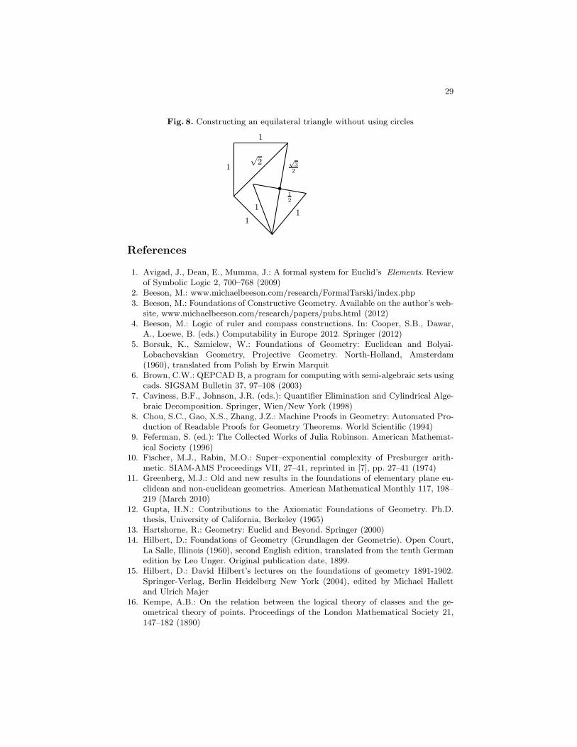
The fourth challenge problem is as follows: Prove from A1-A10 that it is pos-sible to construct an equilateral triangle on a given base. That is, prove Euclid I.1without using circles. Hilbert raised the problem of making such a construction,and gave a solution, in his 1898 “vacation course” [15], page 169. Hilbert’s solu-tion is quite simple; it is based only on constructing perpendiculars and bisectingsegments. One successively constructs right triangles with hypotenuses of length√

2,√

3,√

3/2, as shown in Fig. 8. Since Chapter 8 of Szmielew has the re-quired constructions of perpendiculars and midpoints, we might be in a positionto try to get an Otter proof corresponding to Hilbert’s construction. But thereis a piece of analytic geometry at the end, involving the Pythagorean theorem,which requires the parallel postulate A10. To get a proof from A1-A10, one willcertainly have to use the parallel axiom, because the theorem (as Hilbert knew)is not true in all Hilbert planes, i.e. does not follow from A1-A9. See for example[13], Exercise 39.31, p. 373. We tried this problem by giving Otter the diagramfor Hilbert’s construction, but so far to no avail. We could only apply a 1990technique, because we have no idea what resonators to use. If the program sug-gested in this paper could be carried through, we could back-translate Hilbert’sproof from analytic geometry to A1-A10.

29

Fig. 8. Constructing an equilateral triangle without using circles

b

1

1

√

2

1

11

1

2

√

3

2

References

1. Avigad, J., Dean, E., Mumma, J.: A formal system for Euclid’s Elements. Reviewof Symbolic Logic 2, 700–768 (2009)

2. Beeson, M.: www.michaelbeeson.com/research/FormalTarski/index.php3. Beeson, M.: Foundations of Constructive Geometry. Available on the author’s web-

site, www.michaelbeeson.com/research/papers/pubs.html (2012)4. Beeson, M.: Logic of ruler and compass constructions. In: Cooper, S.B., Dawar,

A., Loewe, B. (eds.) Computability in Europe 2012. Springer (2012)5. Borsuk, K., Szmielew, W.: Foundations of Geometry: Euclidean and Bolyai-

Lobachevskian Geometry, Projective Geometry. North-Holland, Amsterdam(1960), translated from Polish by Erwin Marquit

6. Brown, C.W.: QEPCAD B, a program for computing with semi-algebraic sets usingcads. SIGSAM Bulletin 37, 97–108 (2003)

7. Caviness, B.F., Johnson, J.R. (eds.): Quantifier Elimination and Cylindrical Alge-braic Decomposition. Springer, Wien/New York (1998)

8. Chou, S.C., Gao, X.S., Zhang, J.Z.: Machine Proofs in Geometry: Automated Pro-duction of Readable Proofs for Geometry Theorems. World Scientific (1994)

9. Feferman, S. (ed.): The Collected Works of Julia Robinson. American Mathemat-ical Society (1996)

10. Fischer, M.J., Rabin, M.O.: Super–exponential complexity of Presburger arith-metic. SIAM-AMS Proceedings VII, 27–41, reprinted in [7], pp. 27–41 (1974)

11. Greenberg, M.J.: Old and new results in the foundations of elementary plane eu-clidean and non-euclidean geometries. American Mathematical Monthly 117, 198–219 (March 2010)

12. Gupta, H.N.: Contributions to the Axiomatic Foundations of Geometry. Ph.D.thesis, University of California, Berkeley (1965)

13. Hartshorne, R.: Geometry: Euclid and Beyond. Springer (2000)14. Hilbert, D.: Foundations of Geometry (Grundlagen der Geometrie). Open Court,

La Salle, Illinois (1960), second English edition, translated from the tenth Germanedition by Leo Unger. Original publication date, 1899.

15. Hilbert, D.: David Hilbert’s lectures on the foundations of geometry 1891-1902.Springer-Verlag, Berlin Heidelberg New York (2004), edited by Michael Hallettand Ulrich Majer

16. Kempe, A.B.: On the relation between the logical theory of classes and the ge-ometrical theory of points. Proceedings of the London Mathematical Society 21,147–182 (1890)

30

17. Marchisotto, E.A., Smith, J.T.: The Legacy of Mario Pieri in Geometry and Arith-metic. Birkhauser, Boston, Basel, Berlin (2007)

18. McCharen, J., Overbeek, R., Wos, L.: Problems and experiments for and withautomated theorem-proving programs. IEEE Transactions on Computers C-25(8),773–782 (1976)

19. Mollerup, J.: Die Beweise der ebenen Geometrie ohne Benutzung der Gleichheitund Unbleichheit der Winkel. Mathematische Annalen 58, 479–496 (1904)

20. Narboux, J.: Mechanical theorem proving in Tarski’s geometry. In: Botana, F.,Recio, T. (eds.) Automated Deduction in Geometry: 6th International Workshop,ADG 2006, Pontevedra, Spain, August 31-September 2, 2006, Revised Papers. pp.239–156. Lecture Notes in Artificial Intelligence, Springer (2008)

21. Pasch, M.: Vorlesung uber Neuere Geometrie. Teubner, Leipzig (1882)22. Pasch, M., Dehn, M.: Vorlesung uber Neuere Geometrie. B. G. Teubner, Leipzig

(1926), the first edition (1882), which is the one digitized by Google Scholar, doesnot contain the appendix by Dehn.

23. Pejas, W.: Die Modelle des Hilbertschen Axiomensystems der absoluten Geometrie.Mathematische Annalen 143, 212–235 (1961)

24. Pieri, M.: La geometry elementare istituita sulle nozioni di “punto” e “sfera” (ele-mentary geometry based on the notions of point and sphere). Memorie di matem-atica e di fisica della Societa Italiana delle Scienze 15, 345–450 (1908), englishtranslation in [17], pp. 160–288

25. Quaife, A.: Automated development of Tarski’s geometry. Journal of AutomatedReasoning 5, 97–118 (1989)

26. Quaife, A.: Automated Development of Fundamental Mathematical Theories.Springer, Berlin Heidelberg New York (1992)

27. Renegar, J.: Recent progress on the complexity of the decision problem for thereals. DIMACS Series 6, 287–308, reprinted in [7], pp. 220–241 (1991)

28. Robinson, J.: Definability and decision problems in arithmetic. Journal of SymbolicLogic 14, 98–114, reprinted in [9], pp.7–24 (1949)

29. Schwabhauser, W., Szmielew, W., Tarski, A.: Metamathematische Methoden inder Geometrie: Teil I: Ein axiomatischer Aufbau der euklidischen Geometrie. TeilII: Metamathematische Betrachtungen (Hochschultext). Springer–Verlag (1983),reprinted 2012 by Ishi Press, with a new foreword by Michael Beeson.

30. Strommer, J.: uber die Kreisaxiome. Periodica Mathematica Hungarica 4, 3–16(1973)

31. Tarski, A.: What is elementary geometry? In: Henkin, L., Suppes, P., Tarksi, A.(eds.) The axiomatic method, with special reference to geometry and physics. Pro-ceedings of an International Symposium held at the Univ. of Calif., Berkeley, Dec.26, 1957–Jan. 4, 1958. pp. 16–29. Studies in Logic and the Foundations of Math-ematics, North-Holland, Amsterdam (1959), available as a 2007 reprint, BrouwerPress, ISBN 1-443-72812-8

32. Tarski, A., Givant, S.: Tarski’s system of geometry. The Bulletin of Symbolic Logic5(2), 175–214 (June 1999)

33. Veblen, O.: A system of axioms for geometry. Transactions of the American Math-ematical Society 5, 343–384 (1904)

34. Wos, L.: Automated reasoning and the discovery of missing and elegant proofs.Rinton Press, Paramus, New Jersey (2003)

35. Wu, W.T.: Mechanical Theorem Proving in Geometries: Basic Principles. Springer-Verlag, Wien/ New York (1994)

36. Ziegler, M.: Einige unentscheidbare korpertheorien. Enseignement Math. 2(28),269–280 (1982)