Projective Geometry and Camera Models
34
Projective Geometry and Camera Models ENEE 731 Image Understanding Kaushik Mitra
-
Upload
salvador-gilmore -
Category
Documents
-
view
73 -
download
5
description
Projective Geometry and Camera Models. ENEE 731 Image Understanding Kaushik Mitra. Camera. 3D to 2D mapping 2D to 3D mapping. Preliminaries. Projective geometry Projective spaces ( P 2 ) Homogenous coordinates Projective transformations (Homography). Why Projective Geometry?. - PowerPoint PPT Presentation
Transcript of Projective Geometry and Camera Models
Projective Geometry and Camera Models
ENEE 731 Image Understanding Kaushik Mitra
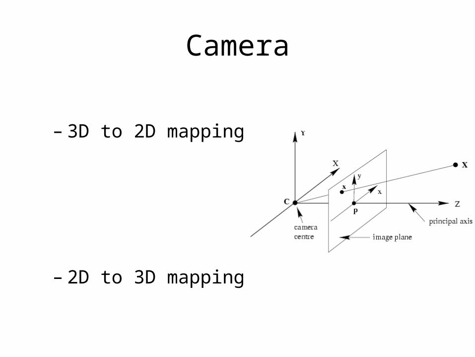
Camera
– 3D to 2D mapping
– 2D to 3D mapping
Preliminaries
• Projective geometry– Projective spaces (P2)– Homogenous coordinates– Projective transformations (Homography)
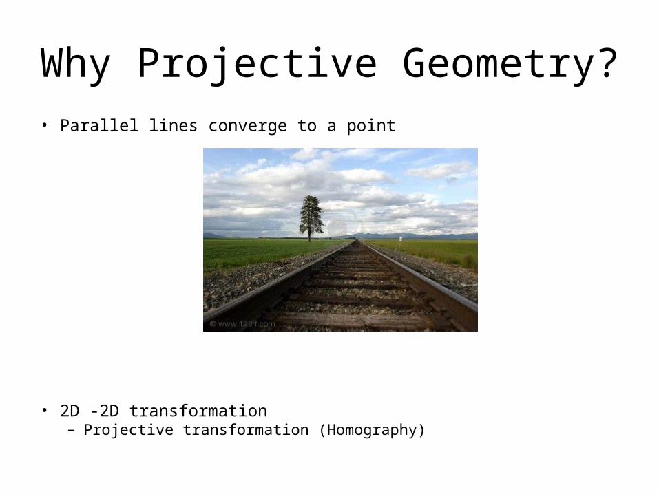
Why Projective Geometry?• Parallel lines converge to a point
• 2D -2D transformation– Projective transformation (Homography)
Projective space P2
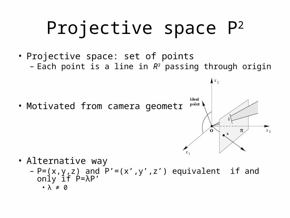
• Projective space: set of points– Each point is a line in R3 passing through origin
• Motivated from camera geometry
• Alternative way– P=(x,y,z) and P’=(x’,y’,z’) equivalent if and only if P=λP’
• λ ≠ 0
P2=R2 U P1
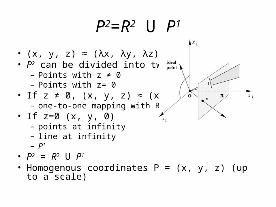
• (x, y, z) ≈ (λx, λy, λz)• P2 can be divided into two subsets
– Points with z ≠ 0– Points with z= 0
• If z ≠ 0, (x, y, z) ≈ (x/z, y/z, 1) – one-to-one mapping with R2
• If z=0 (x, y, 0) – points at infinity– line at infinity– P1
• P2 = R2 U P1
• Homogenous coordinates P = (x, y, z) (up to a scale)
Projective Transformation (Homography)
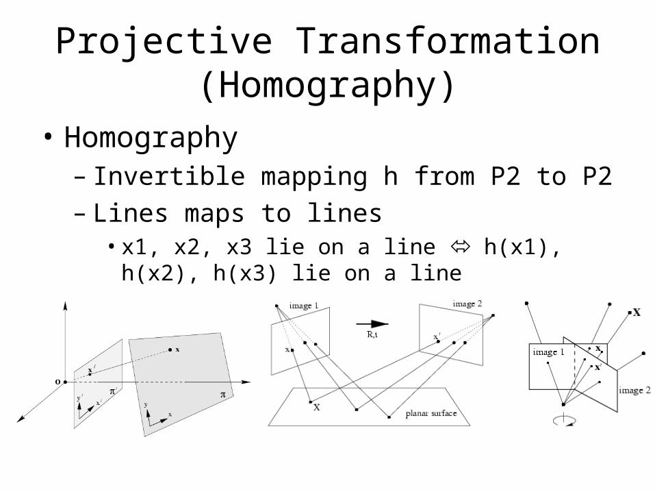
• Homography– Invertible mapping h from P2 to P2– Lines maps to lines• x1, x2, x3 lie on a line h(x1), h(x2), h(x3) lie on a line
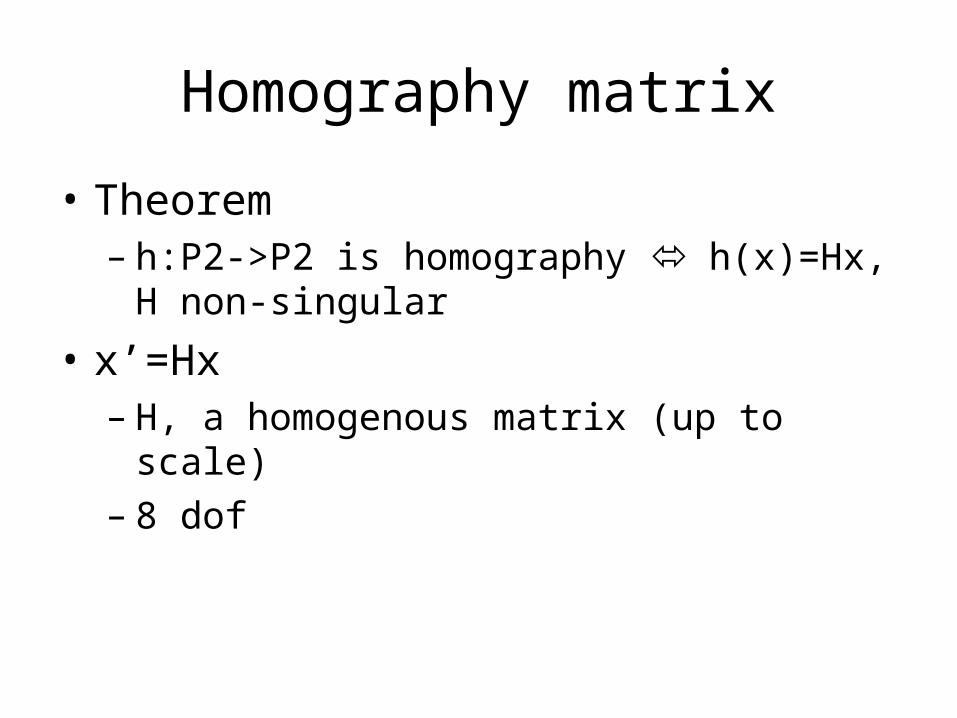
Homography matrix
• Theorem– h:P2->P2 is homography h(x)=Hx, H non-
singular
• x’=Hx– H, a homogenous matrix (up to scale)– 8 dof
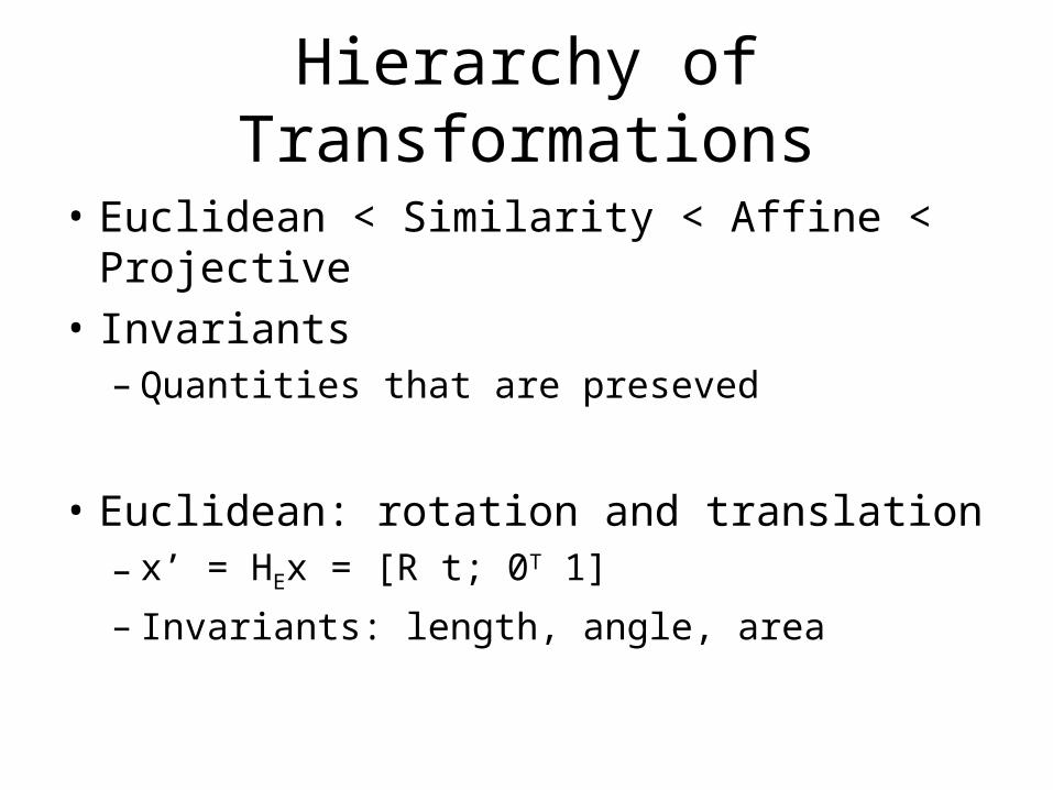
Hierarchy of Transformations
• Euclidean < Similarity < Affine < Projective• Invariants– Quantities that are preseved
• Euclidean: rotation and translation– x’ = HEx = [R t; 0T 1]
– Invariants: length, angle, area
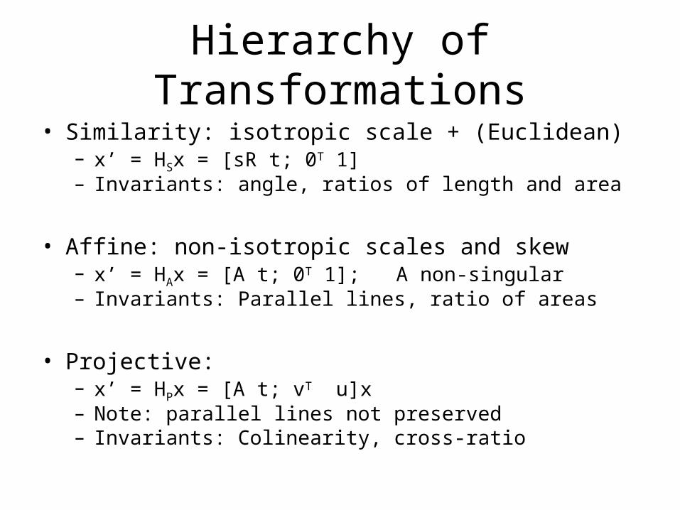
Hierarchy of Transformations• Similarity: isotropic scale + (Euclidean)
– x’ = HSx = [sR t; 0T 1]– Invariants: angle, ratios of length and area
• Affine: non-isotropic scales and skew– x’ = HAx = [A t; 0T 1]; A non-singular– Invariants: Parallel lines, ratio of areas
• Projective: – x’ = HPx = [A t; vT u]x– Note: parallel lines not preserved– Invariants: Colinearity, cross-ratio
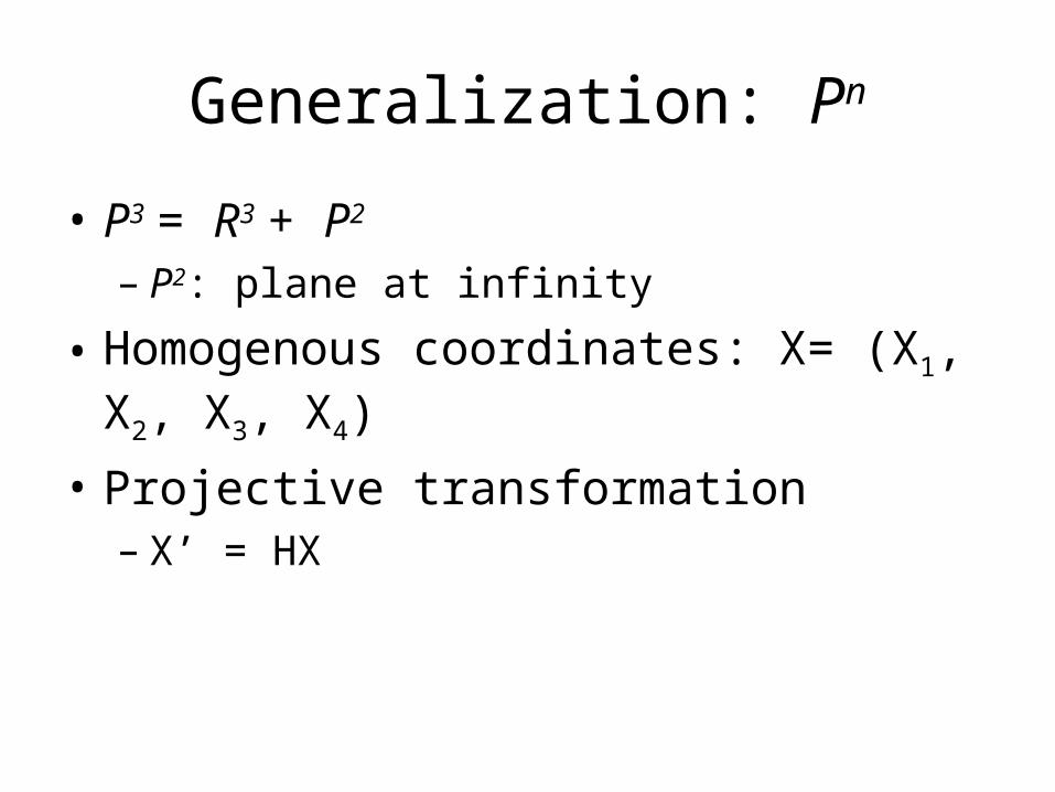
Generalization: Pn
• P3 = R3 + P2
– P2: plane at infinity
• Homogenous coordinates: X= (X1, X2, X3, X4)
• Projective transformation– X’ = HX
Camera Models
Camera Models
• Mapping 3D to 2D: Camera Matrices• Central projection– Pin-hole camera– Finite projective camera
• Parallel projection– Orthographic camera– Affine camera
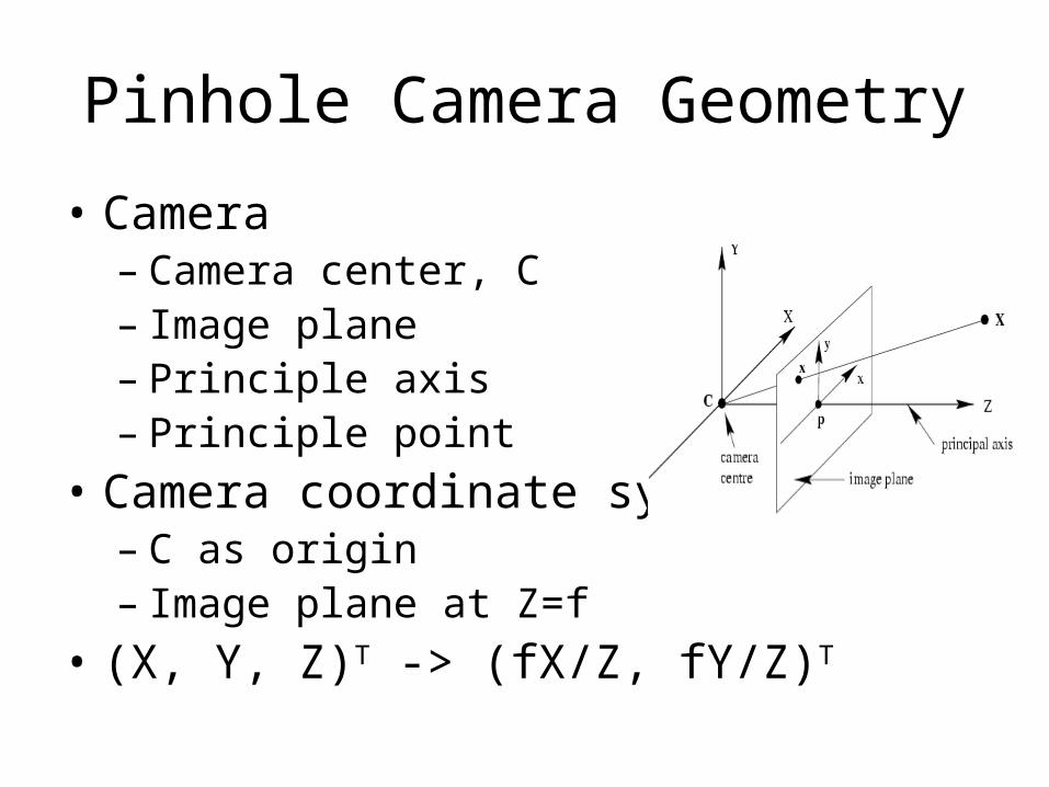
Pinhole Camera Geometry
• Camera– Camera center, C– Image plane– Principle axis– Principle point
• Camera coordinate system– C as origin– Image plane at Z=f
• (X, Y, Z)T -> (fX/Z, fY/Z)T
Camera Matrix
• (X, Y, Z)T -> (fX/Z, fY/Z)T
• Homogenous coordinates– (X, Y, Z, 1)T -> (fX, fY, Z)T
• Transformation: diag(f f 1)[I | 0]• Camera projection matrix: x= PX– P = diag(f, f, 1)[I | 0 ], a 3×4 matrix
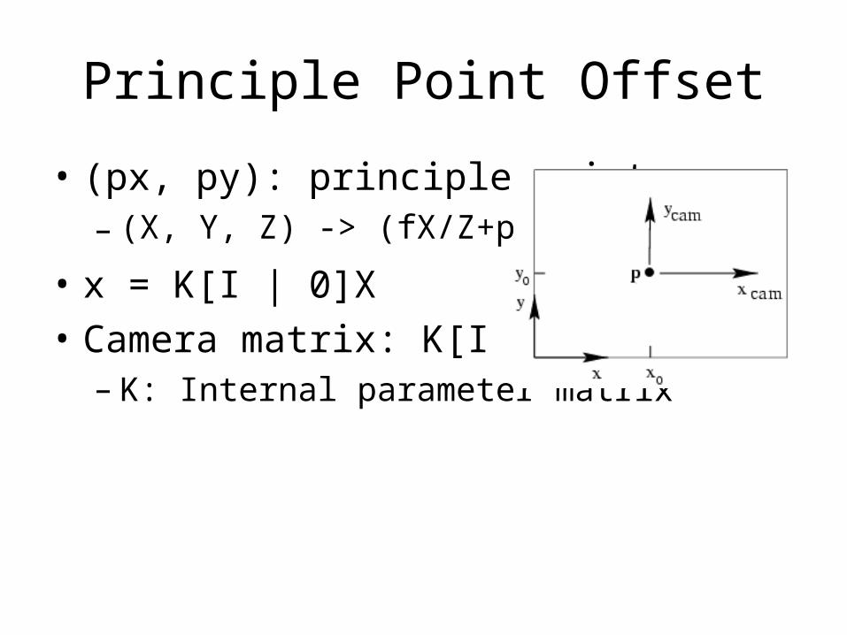
Principle Point Offset
• (px, py): principle point– (X, Y, Z) -> (fX/Z+px, fY/Z+py)
• x = K[I | 0]X• Camera matrix: K[I | 0]– K: Internal parameter matrix
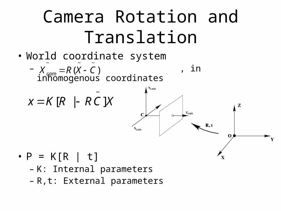
Camera Rotation and Translation
• World coordinate system– , in inhomogenous coordinates
• P = K[R | t]– K: Internal parameters– R,t: External parameters
)(~~~
CXRX cam
XCRRKx ]|[~
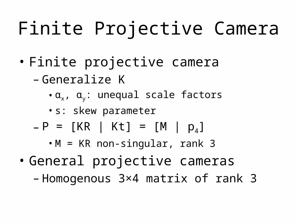
Finite Projective Camera
• Finite projective camera– Generalize K• αx, αy: unequal scale factors
• s: skew parameter
– P = [KR | Kt] = [M | p4]• M = KR non-singular, rank 3
• General projective cameras– Homogenous 3×4 matrix of rank 3
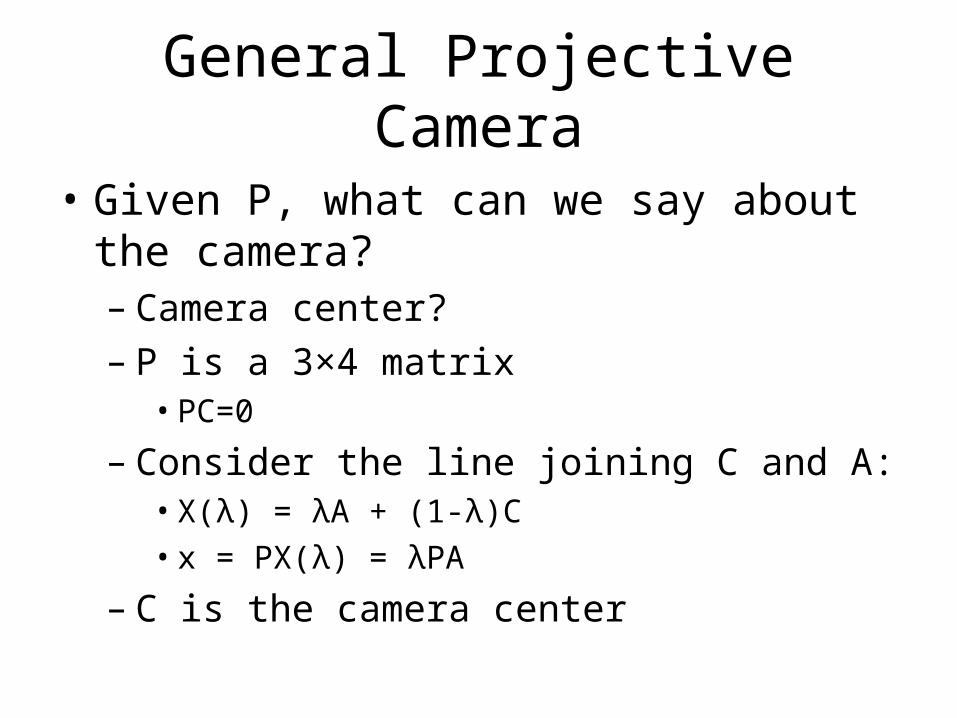
General Projective Camera
• Given P, what can we say about the camera?– Camera center?– P is a 3×4 matrix• PC=0
– Consider the line joining C and A: • X(λ) = λA + (1-λ)C • x = PX(λ) = λPA
– C is the camera center
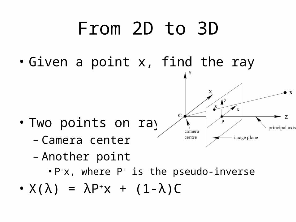
From 2D to 3D
• Given a point x, find the ray
• Two points on ray– Camera center– Another point• P+x, where P+ is the pseudo-inverse
• X(λ) = λP+x + (1-λ)C
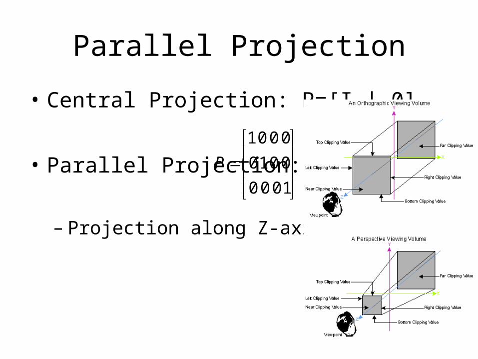
Parallel Projection
• Central Projection: P=[I | 0]
• Parallel Projection:
– Projection along Z-axis
1000
0010
0001
P
Hierarchy of Parallel Projection
• Orthographic projection• Scaled orthographic projection• Weak perspective projection• Affine projection
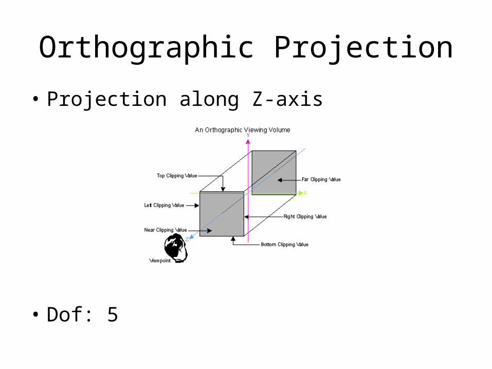
Orthographic Projection
• Projection along Z-axis
• Dof: 5
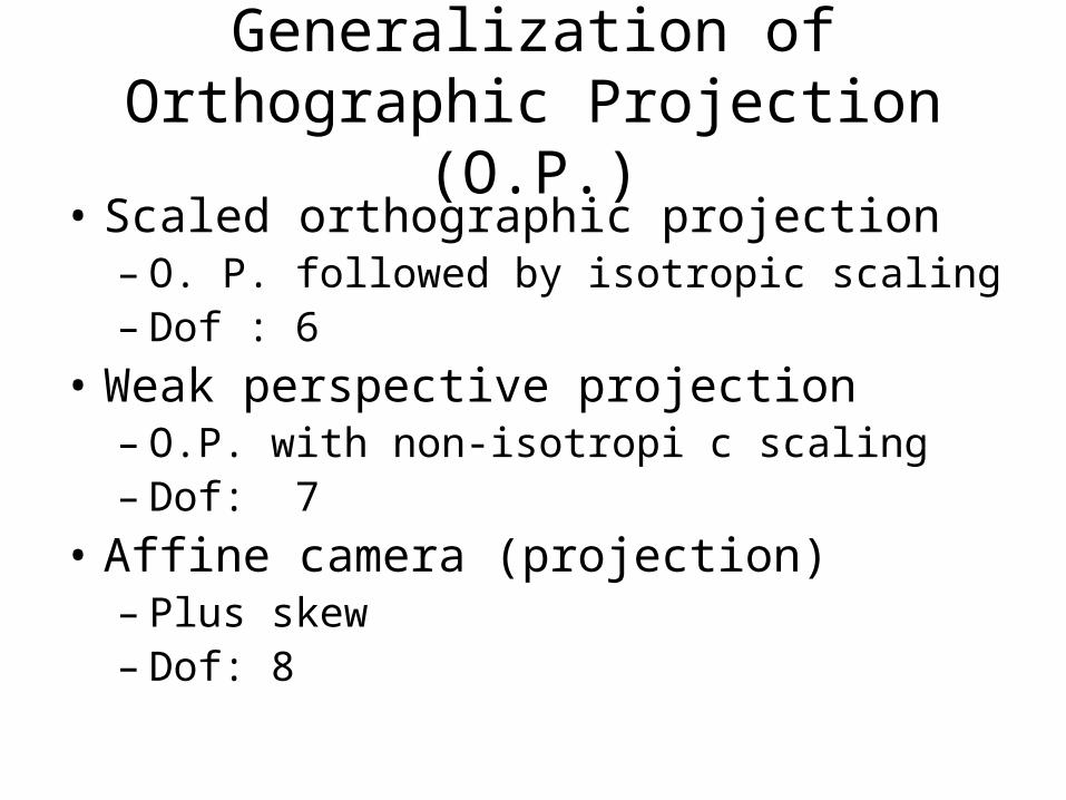
Generalization of Orthographic Projection (O.P.)
• Scaled orthographic projection– O. P. followed by isotropic scaling– Dof : 6
• Weak perspective projection– O.P. with non-isotropi c scaling– Dof: 7
• Affine camera (projection)– Plus skew – Dof: 8

Properties of Affine Camera
• Last row is (0 0 0 1)– Parallel world line maps to parallel image lines
• Camera center at infinity
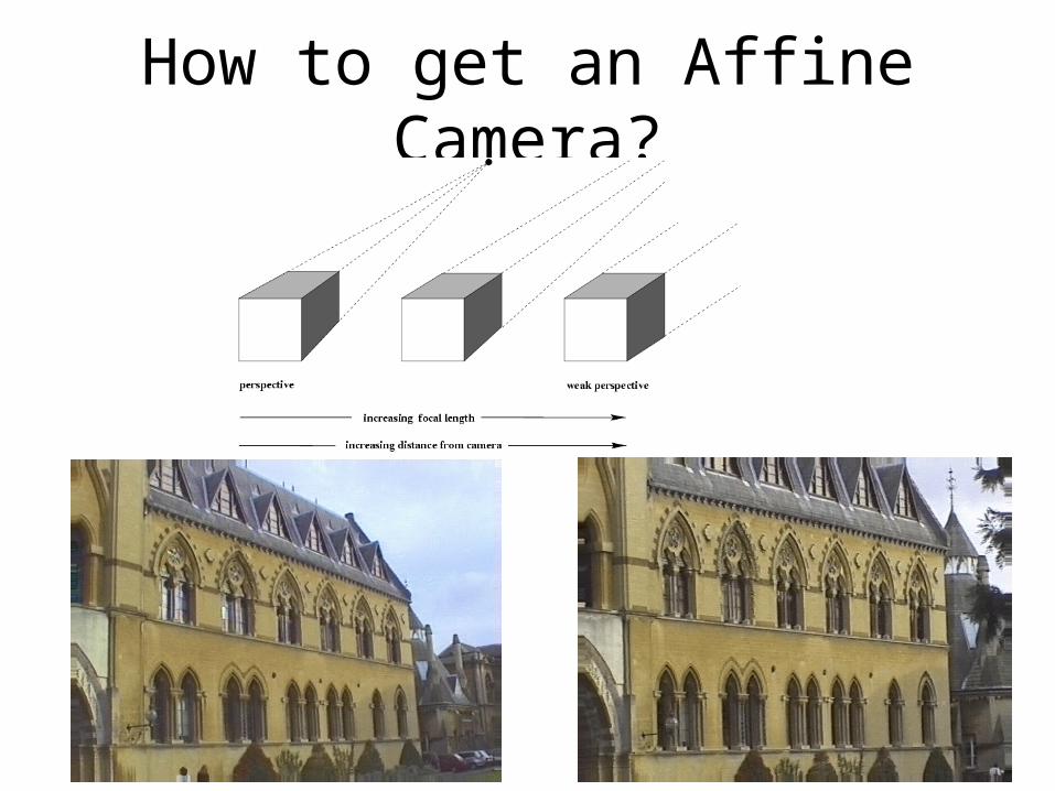
How to get an Affine Camera?
Computation of Camera Matrix P
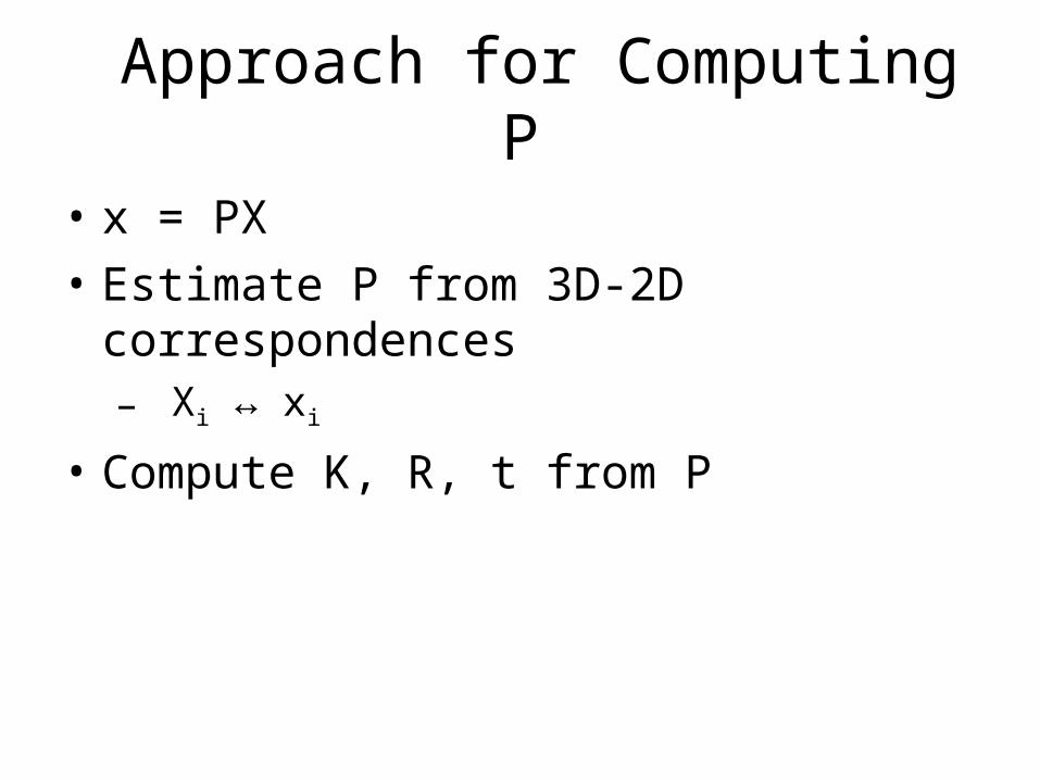
Approach for Computing P
• x = PX• Estimate P from 3D-2D correspondences– Xi ↔ xi
• Compute K, R, t from P
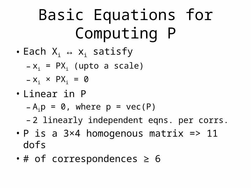
Basic Equations for Computing P
• Each Xi ↔ xi satisfy– xi = PXi (upto a scale)
– xi × PXi = 0
• Linear in P– Aip = 0, where p = vec(P)
– 2 linearly independent eqns. per corrs.
• P is a 3×4 homogenous matrix => 11 dofs• # of correspondences ≥ 6
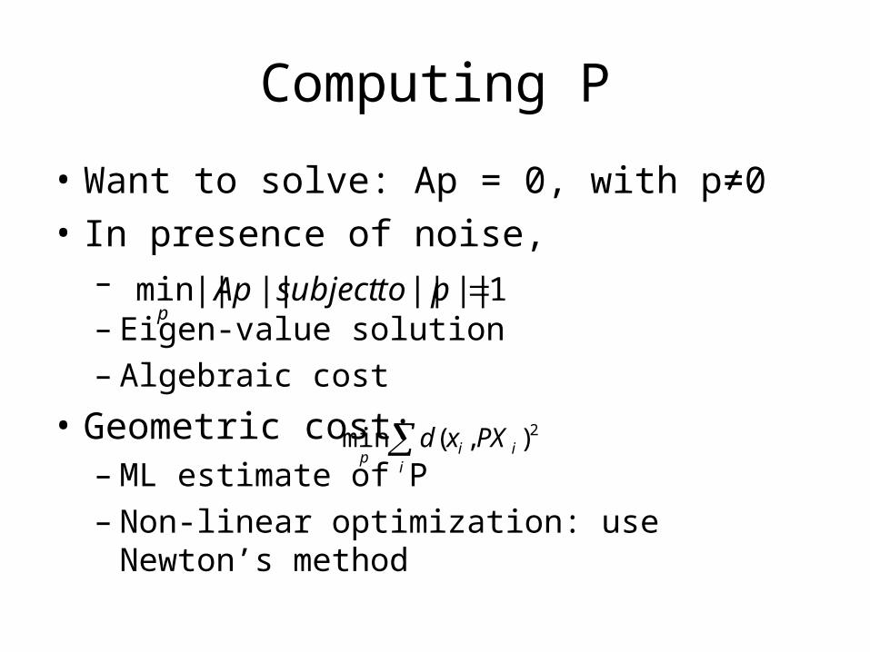
Computing P
• Want to solve: Ap = 0, with p≠0• In presence of noise,– – Eigen-value solution– Algebraic cost
• Geometric cost:– ML estimate of P– Non-linear optimization: use Newton’s method
1||||||||min ptosubjectApp
i
iip
PXxd 2),(min
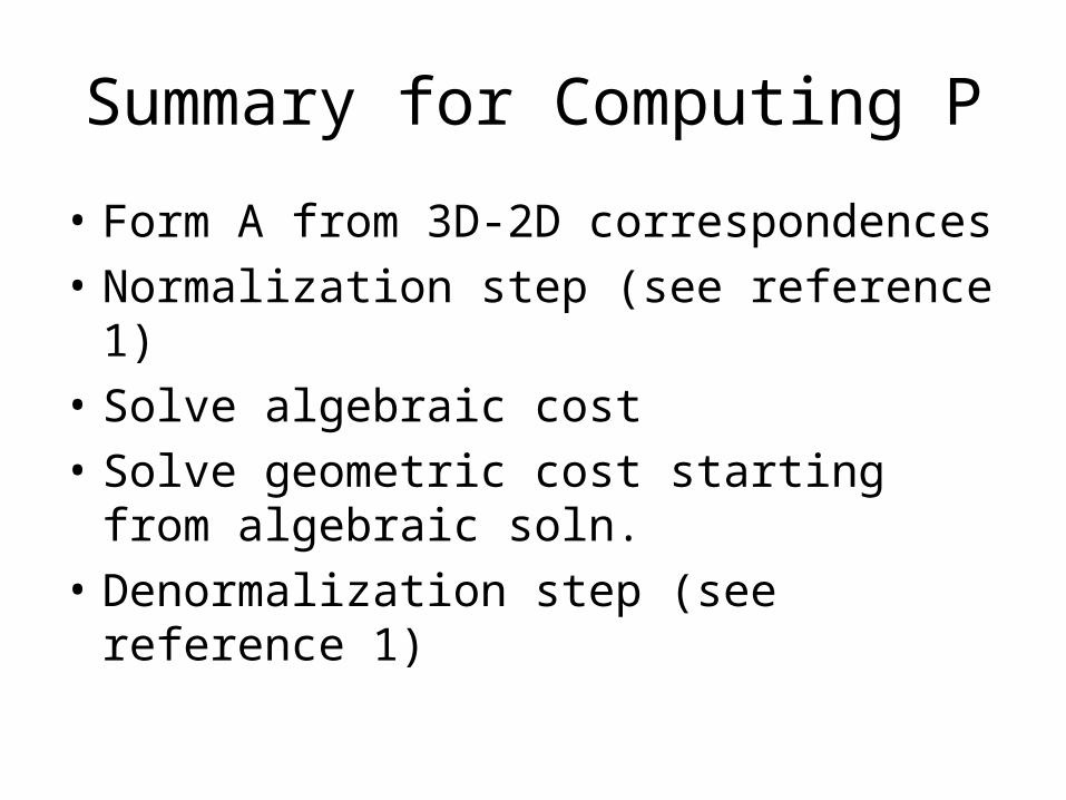
Summary for Computing P
• Form A from 3D-2D correspondences• Normalization step (see reference 1)• Solve algebraic cost• Solve geometric cost starting from algebraic
soln.• Denormalization step (see reference 1)
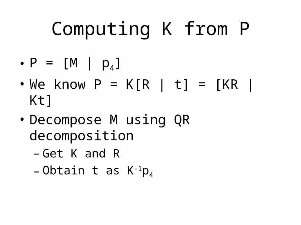
Computing K from P
• P = [M | p4]
• We know P = K[R | t] = [KR | Kt] • Decompose M using QR decomposition– Get K and R– Obtain t as K-1p4
Summary
• Projective geometry: P2 and P3
• Camera models– Central projection (Pin hole camera)– Parallel projection (affine camera)
• Estimation of Camera Model P– Estimation of internal parameter K
References
• 1) Multi-view Geometry (Ch 2, 6, 7)– Hartley and Zisserman
• 2) Computer Vision: Algorithms and Applications– Richard Szeliski