Project work: Modelling of chemical batch reactor - … · Project work: Modelling of chemical...

CFD with OpenSource software

A course at Chalmers University of TechnologyTaught by Hakan Nilsson

Project work:

Modelling of chemical batch reactor

Developed for OpenFOAM-2.4x

Author:Rajukiran Antham

Peer reviewed by:Sankar MenonHakan Nilsson

Disclaimer: This is a student project work, done as part of a course where OpenFOAM and someother OpenSource software are introduced to the students. Any reader should be aware that it

might not be free of errors. Still, it might be useful for someone who would like learn some detailssimilar to the ones presented in the report and in the accompanying files. The material has gone

through a review process. The role of the reviewer is to go through the tutorial and make sure thatit works, that it is possible to follow, and to some extent correct the writing. The reviewer has no

responsibility for the contents.

January 26, 2016

CONTENTS CONTENTS

Contents

1 Introduction 2

2 Meshing 22.1 Meshing Procedure . . . . . . . . . . . . . . . . . . . . . . . . . . . . . . . . . . . . . 4

2.1.1 Stator . . . . . . . . . . . . . . . . . . . . . . . . . . . . . . . . . . . . . . . . 52.1.2 Rotor . . . . . . . . . . . . . . . . . . . . . . . . . . . . . . . . . . . . . . . . 72.1.3 Combining both Meshes . . . . . . . . . . . . . . . . . . . . . . . . . . . . . . 9

3 Setting up case using MRF 103.1 Pre-processing . . . . . . . . . . . . . . . . . . . . . . . . . . . . . . . . . . . . . . . 113.2 Results . . . . . . . . . . . . . . . . . . . . . . . . . . . . . . . . . . . . . . . . . . . . 16

4 Setting up case using sliding grid 174.1 Pre-processing . . . . . . . . . . . . . . . . . . . . . . . . . . . . . . . . . . . . . . . 174.2 Results . . . . . . . . . . . . . . . . . . . . . . . . . . . . . . . . . . . . . . . . . . . . 19

5 Scalar Transport equation 195.1 Implementation in simpleFoam . . . . . . . . . . . . . . . . . . . . . . . . . . . . . . 205.2 Running MRF case with modified solver . . . . . . . . . . . . . . . . . . . . . . . . . 225.3 Implementation in pimpleDyMFoam . . . . . . . . . . . . . . . . . . . . . . . . . . . 25

6 Conclusions 276.1 Meshing . . . . . . . . . . . . . . . . . . . . . . . . . . . . . . . . . . . . . . . . . . . 276.2 Physical Modelling of rotation . . . . . . . . . . . . . . . . . . . . . . . . . . . . . . . 27

7 Appendix 28

i

CONTENTS CONTENTS

Learning outcomes

• Using cfMesh to generate Mesh for this case and learning how to work with cfMesh.

• Physical modelling of rotation using MRF.

• Physical modelling of rotation using mesh motion.

• Implementation of scalar transport equation representing concentration.

• Implementation of probes at point locations to check mixing statistics.

1

2 MESHING

1 Introduction

The purpose of the project is to look at the suitability, pros and cons for alternative techniquesavailable in OpenFOAM for modelling of rotating impeller and static baffles in a reactor. One morepurpose is also to evaluate the use of cfMesh to generate mesh for this application.

In Chemical engineering, chemical reactors are the vessels designed to contain chemical reactions.Vessels which are widely used in the process industries are generally called batch reactors. A typicalbatch reactor consists of a tank with an agitator and a heating or cooling system. They may alsocontain static baffles depending on the application. These vessels may vary in size from less than 1litre to 15000 litres. Batch reactors are used for a variety of operations such as solids dissolution,product mixing, chemical reactions, batch distillation and crystallization.

In this tutorial a lab scale reactor is used. This vessels are in sizes of about 500 to 1000 millilitres.They are used in production systems which are used for preparing small volumes of medical sub-stances. The difficulty in modelling this kind of reactors is modelling of rotation. In OpenFOAMmodelling of rotation is handled using three techniques Single reference frame (SRF), Multiple refer-ence frame and Sliding grid technique. In this tutorial MRF and Sliding grid technique are used. InMRF method a separate rotating region is defined and modelled using rotating frame of reference.Most OpenFOAM steady state solvers are capable of handling MRF using fvOptions. In Sliding gridtechnique, reactor is divided into two regions stationary and a rotating region. The rotating regionis rotated using sliding grid technique and therefore transient problems with strong rotor-statorinteraction can be solved.

Figure 1 shows the geometry of batch reactor. It consists of a reactor vessel of radius 50 mm andheight 90mm. The reactor Vessel contains a stationary baffle rod with a baffle wing attached to it.Impeller is attached to a rotating shaft . The small rotating shaft is attached to a long shaft whichis stationary. The region around the impeller is the MRF region.

Figure 1: Geometry of reactor

2 Meshing

cfMesh was used to generate mesh. cfMesh is an open source library for automatic mesh generationbuilt on top of OpenFOAM. It is compatible with all recent versions of OpenFOAM and FOAM-extend. cfMesh is currently available for following work flows. The mesher operates on triangulatedgeometry inputs in one of the formats fms, ftr and stl. It builds meshes using the choice of basic

2

2 MESHING

a) b)

Figure 2: Geometry divided into two regions a) stator and b) rotor

meshing strategies:

• CartesianMesh - Used to generate 3D hexahedral cells with polyhedral cells in the transitionregions between the cells of different sizes. The meshing process can be started by typingcartesianMesh in the console.

• Cartesian2DMesh - Used to generate 2D meshes. By default cfMesh will generate a bound-ary layer which can be further refined. Meshing process can be started by typing cartesian2DMesh

in the console.

• Tetrahedral - Used to generate tetrahedral cells. By default it does not generate any bound-ary layer but such can be generated later using refinement settings. The meshing process canbe started by typing tetMesh in the console.

• Polyhedral - Used to generate meshes with arbitrary polyhedral cells. It can be used forpoor geometries. The meshing process can be started by typing pMesh in console.

All sharp features in the geometry must be defined prior to the meshing process. The edges at theborder between the two patches are treated as sharp features in the meshing process. This sharpedges are captured only if there is an edge of a triangulation surface at that location.

An STL file describes a raw unstructured triangulated surface by the unit normal vertices of thetriangles using a threedimensional Cartesian coordinate system. They describe only the surfacegeometry without any representation of color or texture. The STL file formats specifies both ASCIIand binary representations. Below is an example of STL file in ASCII representation.

solid xx

facet normal 1.954537e-01 8.563388e-01 4.779976e-01

outer loop

vertex -3.547176e+01 -4.186972e+00 1.980803e+01

vertex -3.639162e+01 -3.977019e+00 1.980803e+01

vertex -3.603364e+01 -4.528674e+00 2.064995e+01

endloop

endfacet

endsolid xx

In the above file xx is a patch name. A patch always starts with solid Name and ends withendsolid Name. Giving name for the patch is not compulsory. Two STL files can be joinedtogether by just copying the contents of one file to other. In the below example, an STL file whichcontains patch YY is added to the above STL file.

solid xx

facet normal 1.954537e-01 8.563388e-01 4.779976e-01

3

2.1 Meshing Procedure 2 MESHING

outer loop

vertex -3.547176e+01 -4.186972e+00 1.980803e+01

vertex -3.639162e+01 -3.977019e+00 1.980803e+01

vertex -3.603364e+01 -4.528674e+00 2.064995e+01

endloop

endfacet

endsolid xx

solid YY

facet normal 4.201081e-01 8.723634e-01 2.499825e-01

outer loop

vertex -3.701545e+01 -4.185124e+00 2.064995e+01

vertex -3.761253e+01 -4.157825e+00 2.155811e+01

vertex -3.662183e+01 -4.634923e+00 2.155811e+01

endloop

endfacet

endsolid YY

We can also split an STL file into different STL files by just copying all triangles of a single patchto a new text file. Two patches can also be combined into a single patch by just copying trianglesof a patch into other patch.

The CartesianMesh strategy is used to generate the mesh in this particular case. cfMesh generatesthe mesh based on the settings given in the meshDict file which is present in the system directory.cfMesh requires only two mandatory settings to start the meshing process:

• surfaceFile - this files points to the file that contains triangulated geometry and the path ofthe file is same as the path of the case directory.

• maxCellSize - this represents the default cell size used for the meshing. It is the maximum cellsize generated in the domain.

cfMesh has number of refinement settings that can be used to generate a good mesh. All the refine-ment settings are not explained in the report. They are explained in detail in the cfMesh user guide.

cfMesh generates the mesh in a single domain. If there are multiple disconnected domains, cfMeshkeeps the region which contains the most number of cells and removes the cells of the other region(s).In the case of a rotorstator simulations it is useful, and in some cases necessary, to generate the meshin more than one region. Therefore the mesh in this case is generated as a single mesh region forrotor and a single mesh region for the stator. These regions are later merged to form the entire mesh.

Given geometry is divided into two regions stator and rotor. Below Table shows how different partsin the geometry are divided into two regions. This can also be seen in Figure 2.

Stator Rotorbaffle rod, baffle wing, stationaryshaft, reactor vessel and MRFinterface

Impeller, rotating shaft, MRFinterface

cfMesh is not installed in OpenFOAM-2.4 X and FOAM-extend 3.1. It can be easily installed byfollowing the instructions given in Appendix.

2.1 Meshing Procedure

The following section explains the meshing procedure for the given geometry. As discussed abovegeometry is divided into two regions. STL files used for generating the mesh are provided alongwith other files.

4


2.1.1 Stator

The following section explains the meshing procedure for stator. This tutorial is based on asmoOctreetutorial in cfMesh tutorials. you can copy asmoOctree tutorial to your run directory by using thecommand

run

cp-r \$FOAM_TUTORIALS/mesh/cartesianMesh/asmoOctree/ stator

It should be noted that cfMesh tutorials are not copied to OpenFOAM tutorials directory whileinstalling it. This should be done manually.

cd stator

rm -r geom.stl

rm -r Allclean

rm -r Allrun

copy stator_updated.stl file from the given files to this directory

vi system/meshDict

Below is the meshDict file of stator. you need to paste this in system/meshDict file. Comments inthe meshDict file will give an idea on different things used in the meshDict file.Below table gives which part corresponds to which patch. As you can see from table reactor vesselis divided into two patches WALL SURFACE and WALL REACTOR and MRF interface is dividedinto three patches TOP,BOTTOM, CYLINDER.

Part Patchreactor vessel WALL SURFACE, WALL REACTORbaffle wing WALL BAFFLE WING,baffle rod WALL BAFFLE RODstationary shaft WALL STAT SHAFTMRF interface TOP, CYLINDER, BOTTOM

renameBoundary is used in the meshDict file to change the patch names and types while generatingmeshes. Here TOP, BOTTOM and CYLINDER patches are renamed to tops, bottoms and cylinders.All other patches are combined into a single patch called stator. localRefinement is used to refinecells at that particular patch. In the meshDict file maxcellSize is specified in meters because cfMeshassumes that the geometry is in meters. The mesh generated will be scaled to required dimensionslater.

surfaceFile "stator_updated.stl";

maxCellSize 2; // [m]

localRefinement //allows for local refinement regions at the boundary

WALL_SURFACE // patch

cellSize 1.2; // requested cell size

WALL_STAT_SHAFT

cellSize 1.2;

WALL_REACTOR

cellSize 2;

5


WALL_BAFFLE_WING

cellSize 1;

refinementThickness 1; // thickness of refinement zone

WALL_BAFFLE_ROD

cellSize 1;

TOP

cellSize 2;

CYLINDER

cellSize 2;

//refinementThickness 1;

BOTTOM

cellSize 2;

//refinementThickness 1;

boundaryLayers //Used to generate boundary layers

patchBoundaryLayers //Used to specify boundary layers for individual patches

WALL_BAFFLE_WING

nLayers 4; // number of layers

thicknessRatio 1.1; // ratio between the thickness of two successive layers

allowDiscontinuity 1;//ensures that number of layers of a patch do not spread to other patches

renameBoundary // used to rename patches

defaultName stator; //default name for all patches

defaultType wall; //default type for all patches

newPatchNames // new patch names

TOP

newName tops; //new Name

type wall; //new Patch Type

BOTTOM

newName bottoms;

type wall;

6


CYLINDER

newName cylinders;

type wall;

The meshing process can be initiated by typing cartesianMesh in the console.

cartesianMesh

improveMeshQuality

checkMesh

improveMeshQuality is used to improve the mesh quality and checkMesh is used to check the qualityof mesh.

2.1.2 Rotor

The meshing procedure for rotor is similar to stator. asmoOctree tutorial should be copied to rundirectory.

run

cp-r $FOAM_TUTORIALS/mesh/cartesianMesh/asmoOctree/ stator

cd stator

rm -r geom.stl

rm -r Allclean

rm -r Allrun

copy rotor_updated.stl file from the given files to this directory

vi system/meshDict

Below table shows which part corresponds to which patch. renameBoundary is used in meshDictfile to rename the patches. New patch Names can also be seen in below table

Part Patch New Patch nameImpeller WALL IMPELLER impellerrotating shaft WALL ROT SHAFT, rshaftMRF interface TOP, CYLINDER,

BOTTOMTOPR, CYLINDERR,

BOTTOMR

Below is meshDict file of rotor.

surfaceFile "rotor_updated.stl";

maxCellSize 1;

localRefinement

WALL_IMPELLER

cellSize 0.8;

WALL_ROT_SHAFT

cellSize 0.5;

TOP

7


cellSize 0.8;

BOTTOM

cellSize 0.8;

CYLINDER

cellSize 0.8;

boundaryLayers

patchBoundaryLayers

WALL_IMPELLER

nLayers 3;

thicknessRatio 1.2;

renameBoundary

newPatchNames

WALL_IMPELLER

newName impeller;

type wall;

WALL_ROT_SHAFT

newName rshaft;

type wall;

CYLINDER

newName CYLINDERR;

type wall;

BOTTOM

newName BOTTOMR;

type wall;

TOP

newName TOPR;

type wall;

8


The meshing process can be initiated by typing cartesianMesh in the console.

cartesianMesh

checkMesh

Figure 3 shows pictures of mesh generated in both stator and rotor regions.

a) b)

Figure 3: Mesh generated using cfMesh in two separate regions a) stator and b) rotor

2.1.3 Combining both Meshes

Now mesh generated in both regions should be combined into a single mesh. This can be done usingmergeMeshes utility in OpenFOAM.

run

cp -r rotor Project

cp -r stator Project

cd Project

mergeMeshes stator rotor

rm -r rotor

cd stator

rm -r constant/polyMesh

mv 1/polyMesh constant/

rm -r 1

In the above commands stator is the master case and rotor is the case that has the mesh to bemerged into the stator mesh. The merged mesh ends up in the master case, in a time directorycorresponding to startTime+deltaT. There is also a flag -overwrite that will force mergeMeshes todirectly rewrite to the constant/polyMesh directory in master case.

run

cp -r rotor Project

cp -r stator Project

cd Project

mergeMeshes -overwrite stator rotor

9

3 SETTING UP CASE USING MRF

The original geometry was generated in millimeters, but cfMesh and OpenFOAM assume that thegeometry is in meters. Therefore the mesh is transformed to meters using

transformPoints -scale '(0.001 0.001 0.001)'

Now we have a domain with two separate regions which are not coupled to each other. This can beseen using the checkMesh command.

checkMesh

Figure 4 is a clip with normal in the Z-direction, at the center of the rotor. Both stator and rotorregions can be seen in the figure.

Figure 4: combined mesh after using mergeMeshes

3 Setting up case using MRF

In MRF approach fluid flow is computed using different reference frames. Rotating zone is solvedin the rotating frame and stationary zone is solved in the stationary frame. This approach accountsthe rotation of the rotor without having to physically rotate any part of the mesh. The approach isalso called the frozen rotor technique. In MRF approach cells in the rotating region should be keptin a separate cellZone. The Navier-Stokes equations are solved in a relative reference frame, as

∂(ur)

∂t+∇ · (urur) + 2Ω× ur + (Ω× (Ω + r)) = −∇(

p

ρ) +∇ · (υ∇ur), (1)

where p, ρ and υ denote pressure, density and kinematic viscosity respectively. The relative velocityur is defined by

ur = u− Ω ∗ r, (2)

and Ω represents the angular velocity.

equ(1) reduces to equ(3) if Ω = 0, which is in the stationary region.

∂(ρu)

∂t+∇ · (ρuu) = −∇p+∇ · (µ∇u) (3)

where µ represents dynamic viscosity.In this case mesh is generated in two regions and merged together using mergeMeshes utility. Theconnection between two regions is handled using a mesh interface. OpenFOAM supports differentmesh interfaces like General Grid interface (GGI), mixing plane and Arbitrary Mesh Interface (AMI).GGI and mixing plane are used only in FOAM-extend. In this case AMI (Arbitrary Mesh Interface) isused. AMI operates by projecting one of the patch faces onto the other. From these weighting factorswill be calculated, to determine how an AMI boundary cell should couple to the AMI boundary cellson the other side of the interface. This weighting factors should be close to 1 always. AMI interfacecan be used even if the patches are not perfectly conformal, but it is better to keep both patches asconformal as possible.

10

3.1 Pre-processing 3 SETTING UP CASE USING MRF

3.1 Pre-processing

The MRF technique is implemented in different ways in OpenFOAM and FOAM-extend. Rotationis defined in system/fvOptions in OpenFOAM and in constant/MRFZones in Foam-extend. Belowtable shows how the MRF technique is implemented in OpenFOAM and FOAM-extend

OpenFOAM FOAM-extendsimpleFoam + fvOptions MRFsimpleFoam + MRFZones

This tutorial is based on the mixerVessel2D tutorial in OpenFOAM-2.4.x. This tutorial can becopied to your run folder by using the command

cp -r $FOAM_TUTORIALS/incompressible/simpleFoam/mixerVessel2D $FOAM_RUN

run

cp -r Project ProjectMRF

cd ProjectMRF

cd stator

vi constant/polyMesh/boundary

Interface between patches of rotor and stator region should be coupled using AMI interface, this canbe done by editing boundary file in constant/polyMesh/boundary

9

(

tops

type cyclicAMI;

inGroups 1(cyclicAMI);

nFaces 1224;

startFace 1174428;

matchTolerance 0.0001;

transform noOrdering;

neighbourPatch TOPR; //neighbor patch on rotor side

bottoms

type cyclicAMI;


nFaces 968;

startFace 1175652;



neighbourPatch BOTTOMR; //neighbor patch on rotor side

cylinders

type cyclicAMI;


nFaces 1376;

startFace 1176620;



neighbourPatch CYLINDERR; //neighbor patch on rotor side

stator

11


type wall;

inGroups 1(wall);

nFaces 27664;

startFace 1177996;

impeller

type wall;

inGroups 1(wall);

nFaces 25320;

startFace 1205660;

rshaft

type wall;

inGroups 1(wall);

nFaces 704;

startFace 1230980;

CYLINDERR

type cyclicAMI;


nFaces 18856;

startFace 1231684;



neighbourPatch cylinders; //neighbor patch on stator side

BOTTOMR

type cyclicAMI;


nFaces 14448;

startFace 1250540;



neighbourPatch bottoms; //neighbor patch on stator side

TOPR

type cyclicAMI;


nFaces 14432;

startFace 1264988;



neighbourPatch tops; //neighbor patch on stator side

)

In the above boundary file tops, bottoms and cylinders are the AMI interfaces on the stator sideand TOPR, BOTTOMR, and CYLINDERR are the AMI interfaces on the rotor side. Each patch

12


should be given a corresponding neighbour patch. Corresponding changes are also to be done in the0 directory.

For example 0/U file is written as

dimensions [0 1 -1 0 0 0 0];

internalField uniform (0 0 0);

boundaryField

rshaft

type fixedValue;

value uniform (0 0 0);

stator

type fixedValue;


impeller

type fixedValue;


TOPR

type cyclicAMI;

value $internalField;

BOTTOMR

type cyclicAMI;


CYLINDERR

type cyclicAMI;


tops

type cyclicAMI;


bottoms

type cyclicAMI;

13



cylinders

type cyclicAMI;


All the files in 0 directory are provided. They can be copied directly from there. This can also bedone by copying the O/files from mixerVessel2D tutorial and doing the corresponding changes.

Next step is to create a cellZone for defining the rotation of the impeller. cfMesh does not automat-ically create cell sets and cell zones while generating meshes. This can be done by using the setSetand topoSet utilities in OpenFOAM and Foam-extend. There are a number of options available inboth setSet and topoSet to do mesh manipulations. In this case both setSet and topoSet are usedto get an idea how both of them work. Since we already have a cellSet of the rotor region which iswritten when checkMesh is done, we can use it directly to create the rotor cellZone using

setSet

cellZoneSet rotor new setToCellZone region1

quit

In the above command rotor is the name of the cellZone and region1 is the cell set which containsall the cells of the rotor region.The next step is to create a faceSet containing all the faces of the AMI interfaces.This is done usingthe topoSet utility and a topoSetDict file. This file is located in system/topoSetDict, and should inthis contain

actions

(

name AMI; // Get both sides of AMI

type faceSet;

action new; // Get all faces in cellSet

source patchToFace;

sourceInfo

name bottoms;

name AMI;

type faceSet;

action add; //Add faces to faceset AMI

source patchToFace;

sourceInfo

name tops;

14


name AMI;

type faceSet;

action add;

source patchToFace;

sourceInfo

name cylinders;

name AMI;

type faceSet;

action add;

source patchToFace;

sourceInfo

name CYLINDERR;

name AMI;

type faceSet;

action add;

source patchToFace;

sourceInfo

name BOTTOMR;

name AMI;

type faceSet;

action add;

source patchToFace;

sourceInfo

name TOPR;

);

The above topoSetDict file is provided along with the case files. In the above topoSetDict file ini-tially faceSet with name AMI is created which contains all the faces of patch bottoms. This is doneby using the action command new. After that all the faces from other patches are added to faceSetAMI using the action command add.

topoSet

The settings for the rotation component in OpenFOAM-2.4.x is defined using the system/fvOptionsfile. Patches which are adjacent to rotating patches and which are non-rotating should be includedin nonRotatingpatches () . As you can see in the below fvOptions file tops, bottoms, and cylinderspatches are non-rotating stator AMI interface patches. Angular velocity of 40 rad/sec along Z-axis

15

3.2 Results 3 SETTING UP CASE USING MRF

is given for the rotating region.Below fvOptions file is provided along with the case files.

MRF1

type MRFSource;

active true;

selectionMode cellZone;

cellZone rotor;

MRFSourceCoeffs

nonRotatingPatches (tops bottoms cylinders);

active true;

origin (0 0 0);

axis (0 0 1);

omega 40; // in rad/sec

fvSchemes, fvSolution and controlDict can be copied from the given case files to system directory.This can also be done by copying this files from mixerVessel2D tutorial, but necessary changes shouldbe done to fvSolution file to implement turbulence model. turbulence properties, RAS propertiesand transport properties files should be added to constant directory to implement turbulence model.This files can be copied from given case files.

Now the set-up for MRF is done and the simulation is started by typing simpleFoam in console.

simpleFoam

3.2 Results

0.25

0.5

0.75

1

U Magnitude

0

1.21

Figure 5: U magnitude at Z=0.0032 m plane

16

4 SETTING UP CASE USING SLIDING GRID

Figure 6: Vector arrows (Umagnitude) representing flow direction

Figure 5 is a velocity contour at Z=0.0032 m plane. From the figure we can see high velocities nearthe tip of the blade which is expected. Velocity magnitude at the tip of the blade is in agreementwith analytical solution which is 1.2 m/s.

V = r ∗ Ω = 0.03 ∗ 40 = 1.2m/s

Figure 6 shows the velocity vectors entering from the top of the impeller and a recirculation regionat the side of the impeller. We can also observe high velocity at the tip of the impeller.

4 Setting up case using sliding grid

The sliding grid method allows adjacent grids to slide relative to each other along the internal inter-face surface. We need to have two mesh regions and an interface that couples the two regions. Usingthis approach the interaction between the stator and rotor can be fully resolved. The pimpleDyM-Foam solver in OpenFOAM is employed to obtain a unsteady solution. This method takes morecomputational time than the MRF technique discussed above. AMI is used as interface between thestator and rotor patches.

4.1 Pre-processing

The setup used for AMI is very much similar to that of MRF. This is because we are using the samemesh interface (AMI) between stator and rotor. We can use the same meshes as MRF. The onlychange is how the mesh motion is defined. Here mesh motion is defined using a dynamicMeshDictfile which is present in constant directory. Here mesh motion is obtained by using solidBodyMo-tionFvMesh class which is a sub class of dynamicFvMesh. To start with the case copy the MRF case

run

cp -r ProjectMRF ProjectAMI

cd constant

Below is the dynamicMeshdict file. This file is provided along with the case files. In the dynam-icMeshDict file cellZone specifies which region to rotate. solidBodyMotionFunction specifies the

17

4.1 Pre-processing 4 SETTING UP CASE USING SLIDING GRID

type of motion. Here angular velocity of 5 rad/sec is taken. Angular velocity should be increasedgradually over time to attain the an angular velocity of 40 rad/sec. The reason behind this is meancourant number. In order to keep the mean courant number low we need to decrease either timestep or angular velocity for a given mesh.

FoamFile

version 2.0;

format ascii;

class dictionary;

location "constant";

object dynamicMeshDict;

// * * * * * * * * * * * * * * * * * * * * * * * * * * * * * * * * * * * * * //

dynamicFvMesh solidBodyMotionFvMesh;

motionSolverLibs ( "libfvMotionSolvers.so" );

solidBodyMotionFvMeshCoeffs

cellZone rotor;

solidBodyMotionFunction rotatingMotion;

rotatingMotionCoeffs

origin (0 0 0);

axis (0 0 1);

omega 5; // rad/s

// ************************************************************************* //

We need to remove constat/fvOptions file from the system directory since we are not defining rotationusing this file. This is not compulsory because we are not using the same solver and pimpleDyM-Foam won’t use MRF settings from that file.

cd ..

rm -r system/fvOptions

Time step to be used in the simulation can be given in controlDict file. we can use adjustTimeStepto decrease the time step during the simulation if the mean courant number is increasing more than1. In this case time step of 1e-4 is used.copy the below controlDict file to system/controlDict file

FoamFile

version 2.0;

format ascii;

class dictionary;

location "system";

object controlDict;

18

4.2 Results 5 SCALAR TRANSPORT EQUATION

// * * * * * * * * * * * * * * * * * * * * * * * * * * * * * * * * * * * * * //

application pimpleDyMFoam;

startFrom latestTime;

startTime 0;

stopAt endTime;

endTime 5;

deltaT 1e-4;

writeControl adjustableRunTime;

writeInterval 0.01;

purgeWrite 10;

writeFormat ascii;

writePrecision 6;

writeCompression off;

timeFormat general;

timePrecision 6;

runTimeModifiable true;

//adjustTimeStep yes;

maxCo 2;

Now the set-up for sliding grid is done and the simulation is started by typing pimpleDyMFoam inconsole.

pimpleDyMFoam

4.2 Results

Figure 7 shows the velocity contours at various time steps. Effect of impeller position on the flowfield can be clearly seen from the figure. Here you can see high velocities near the tip of the impeller.Compared to MRF case we don’t have high velocities in between impeller blades.

5 Scalar Transport equation

Scalar transport equation representing concentration is implemented to check the mixing propertiesof reactor. This is done by introducing a transport equation in the solver.

19

5.1 Implementation in simpleFoam 5 SCALAR TRANSPORT EQUATION

0.4

0.8

1.2

U Magnitude

0

1.31

a) at t=4.925s

0.4

0.8

1.2

U Magnitude

0

1.31

b) at t=4.935s

0.4

0.8

1.2

U Magnitude

0

1.31

c)at t=4.945s

0.4

0.8

1.2

U Magnitude

0

1.31

d) at t=4.955s

Figure 7: Velocity contours at Z=0.0032 m

The scalar transport equation representing concentration is

∂C

∂t+∂(uiC)

∂xi=∂(D ∂C

∂xi)

∂xi+ S, (4)

where C is concentration, D is Diffusion coefficient and S is a source term.

5.1 Implementation in simpleFoam

The scalar transport equation can be implemented done by the following steps.

foam

cp -r --parents applications/solvers/incompressible/simpleFoam $WM_PROJECT_USER_DIR

cd $WM_PROJECT_USER_DIR/applications/solvers/incompressible

mv simpleFoam mysimpleFoam

cd mysimpleFoam

wclean

mv simpleFoam.C mysimpleFoam.C

rm -r SRFSimpleFoam porousSimpleFoam

Allwmake

In the above steps the simpleFoam directory is copied to the user directory and renamed as mysim-pleFoam. simpleFoam/simpleFoam.C is renamed as mysimpleFoam.C. Now we need to add thetransport equation in mysimpleFoam.C file before runTime.write().

volScalarField alphaEff("alphaEff", turbulence->nu()/Sc + turbulence->nut()/Sct);

solve (fvm::ddt(C)+fvm::div(phi, C)-fvm::laplacian(alphaEff, C));

20

5.1 Implementation in simpleFoam 5 SCALAR TRANSPORT EQUATION

where Sc and Sct are Schmidt’s number and turbulent Schmidt’s number.

Next we should add volumeScalarField C in the createFields.H file. We can copy the same as p andchange p to C, since both are scalar fields. we should also define Sc and Sct, this can be done bydefining it in createFields.H file by adding below code

Info<< "Reading field C\n" << endl;

volScalarField C

(

IOobject

(

"C",

runTime.timeName(),

mesh,

IOobject::MUST_READ,

IOobject::AUTO_WRITE

),

mesh

);

Info<< "Reading transportProperties\n" << endl;

IOdictionary transportProperties

(

IOobject

(

"transportProperties",

runTime.constant(),

mesh,

IOobject::MUST_READ_IF_MODIFIED,

IOobject::NO_WRITE

)

);

dimensionedScalar Sc

(

transportProperties.lookup("Sc")

)

dimensionedScalar Sct

(

transportProperties.lookup("Sct")

)

This code will look for the value of Sc and Sct in a transportPropoerties file in the constant directory.We should also change the name of file in Make/files to compile the modified solver, which can bedone by using the command

string="mysimpleFoam.C\nEXE = \$(FOAM_USER_APPBIN)/mysimpleFoam"

printf "%b\n" "$string" > Make/files

Compile with wmake command in mysimpleFoam directory.

wmake

21

5.2 Running MRF case with modified solver 5 SCALAR TRANSPORT EQUATION

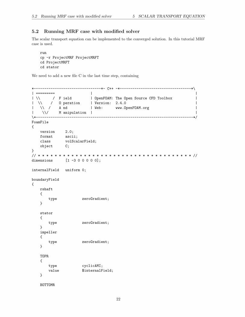
5.2 Running MRF case with modified solver

The scalar transport equation can be implemented to the converged solution. In this tutorial MRFcase is used.

run

cp -r ProjectMRF ProjectMRFT

cd ProjectMRFT

cd stator

We need to add a new file C in the last time step, containing

*--------------------------------*- C++ -*----------------------------------*\

| ========= | |

| \\ / F ield | OpenFOAM: The Open Source CFD Toolbox |

| \\ / O peration | Version: 2.4.0 |

| \\ / A nd | Web: www.OpenFOAM.org |

| \\/ M anipulation | |

\*---------------------------------------------------------------------------*/

FoamFile

version 2.0;

format ascii;

class volScalarField;

object C;

// * * * * * * * * * * * * * * * * * * * * * * * * * * * * * * * * * * * * * //

dimensions [1 -3 0 0 0 0 0];

internalField uniform 0;

boundaryField

rshaft

type zeroGradient;

stator

type zeroGradient;

impeller

type zeroGradient;

TOPR

type cyclicAMI;


BOTTOMR

22


type cyclicAMI;


CYLINDERR

type cyclicAMI;


tops

type cyclicAMI;


bottoms

type cyclicAMI;


cylinders

type cyclicAMI;


// * * * * * * * * * * * * * * * * * * * * * * * * * * * * * * * * * * * * * //

We should also add a dimensioned scalar in the constant/transportProperties file:

Sc Sc [ 0 0 0 0 0 0 0 ] 0.7; //Schmidt's number

Sct Sct [ 0 0 0 0 0 0 0 ] 0.7; //Turbulent Schmidt's number

We should also add a divergence scheme in system/fvSchemes file for C:

div(phi,C) Gauss linearUpwind Gauss;

We should also define the settings for the solution of the linear system for C in fvSolution:

C

solver smoothSolver;

smoother GaussSeidel;

nSweeps 2;

tolerance 1e-08;

relTol 0.1;

We need to initialize C and this can be done by using the setFields utility. We can copy thesetFieldsDict file from damBreak tutorial using the following command

cp $FOAM_TUTORIALS/multiphase/interFoam/laminar/damBreak/system/setFieldsDict system

23


The following changes are made to the setFieldsDict file. I used a cylinderToCell option here to pickup a region to set the field values.

defaultFieldValues

(

volScalarFieldValue C 0

);

regions

(

cylinderToCell

p1 (0 0 0.036); // centre of first circle

p2 (0 0 0.043); // centre of second circe

radius 0.035; // radius of cylinder

fieldValues

(

volScalarFieldValue C 1

);

);

Now C is initialized by running setFields in console.

setFields

I have introduced probes at different point locations in the reactor vessel to look at the concentrationat those locations over iterations. This is done by using probes utility in OpenFOAM. This isimplemented by adding the following code to the controlDict file.

functions

concentraionProbes

type probes;

functionObjectLibs ("libsampling.so");

outputControl timeStep;

outputInterval 1;

probeLocations

(

( 0.010 0.010 0.043 ) // Probe(0) probe locations coordinates

( 0.010 -0.010 0.043 ) // Probe (1)

( 0.010 0.010 -0.010 ) // Probe (2)

);

fields // field to plot

(

C

);

Now the set-up for case is done and simulation is started by typing mysimpleFoam in console.

mysimpleFoam

24

5.3 Implementation in pimpleDyMFoam 5 SCALAR TRANSPORT EQUATION

5.3 Implementation in pimpleDyMFoam

The implementation of a scalar transport equation in pimpleDyMFoam is similar to that describedfor simpleFoam. This is left as an exercise to the reader, but the results will be explained below.

Results

Project AMI case is solved initially till t=4.995 sec to attain convergence. Then the scalar transportequation is introduced and solved for more 0.65 sec. Concentration is plotted at three probe locationsand plotted over time. Location of the probes are given below

Probe 0 ( 0.010 0.010 0.043 ) //(x y z) coordinates

Probe 1 ( 0.010 -0.010 0.043 )

Probe 2 ( 0.010 0.010 -0.010 )

Figure 8: Concentration vs Time

Figure 8 shows the plot of concentration over time. It can be seen from figure that at Probe 2 theconcentration is zero till t=5.1 sec. This is as expected because Probe 2 is at the top of the reactor.Concentration at Probe 0 and 1 is decreasing and attaining a uniform value as time passes. It canalso be seen that concentration at Probe 2 is decreasing from t=5.28 sec and reaching a uniformvalue. In order to achieve a uniform concentration thought the reactor the simulation should becontinued for more time. This is not done because of time constraints.

Figure 9 shows the concentration contours in a plane normal to Y. At t=4.995s the concentration is 1in the middle of the reactor. From the figure it can also be seen how the water is moving downwardsin the reactor. This is as expected because the impeller is located close to the bottom of the reactorvessel. Effect of baffle rod and wing can also be seen from the figures. The concentration at probe2 is almost zero till 5.345s and increases over time to reach a uniform concentration.

25

5.3 Implementation in pimpleDyMFoam 5 SCALAR TRANSPORT EQUATION

0.25

0.5

0.75

C

0

1

a) at t=4.995s

0

0.2

0.4

0.6

0.8

C

-0.00557

0.936

b) at t=5.045s

0.2

0.4

0.6

C

0

0.687

c)at t=5.095s

0.1

0.2

C

0

0.295

d) at t=5.195s

0.1

0.2

C

0

0.245

e) at t=5.245s

0.04

0.08

0.12

C

0

0.155

f) at t=5.345s

0.025

0.05

0.075

0.1C

0

0.101

g) at t=5.445s

0.02

0.04

0.06

0.08

C

0

0.0827

h) at t=5.545s

0.02

0.04

0.06

C

0

0.0749

i) at t=5.645s

Figure 9: Concentration at different times

26

6 CONCLUSIONS

6 Conclusions

6.1 Meshing

cfMesh is a robust and easy to use meshing tool. It can generate hexa, tetra and polyhedral meshes.It can handle bad geometries very well. One of the main advantage is its ability to run in parallelwhich saves lot of time when generating large meshes. The available refinement settings are easy touse. It is very good with handling sharp edges if the given input geometry is good. It is very easyto generate an initial mesh, however it takes some time to generate an ideal mesh.The main disadvantage with cfMesh is, it can’t generate multi region meshes if there are multipledisconnected regions. Even though it is good at handling geometries with poor quality, final meshquality still depends largely on the quality of input geometry.

Below figure shows mesh generated in the rotor region. As you can see from below figure (a), whenthe input geometry is given as a single patch, edges of the rotor region are not captured properly.This problem is solved by dividing the geometry into individual patches. In figure (b) rotor regionis divided into 3 different patches top, bottom and cylinder.

a)with single patch b)with individual patches

Figure 10: Comparison between using a single patch and individual patches

6.2 Physical Modelling of rotation

Physical modelling of rotation is done using two methods MRF and sliding grid. The advantagesand disadvantages of both methods will be discussed in below section.

MRF

MRF is a steady state solution with a fixed impeller position. Hence the name Frozen rotor tech-nique. The main advantage with MRF is, it is not computationally expensive. All steady stateOpenFOAM solvers support MRF and it is easy to implement using fvOptions. One more advan-tage with MRF is, it is not necessary to generate mesh in two regions. The rotor region can be pickedeasily using topoSet and setSet utilities in OpenFOAM. There are number of options available inboth of these utilities to manipulate meshes. It is possible to get an unsteady solution using MRF,but this is not accurate because the stator and rotor interaction cannot be resolved. This is becauseimpeller or rotor is fixed at a single position. It can be used when there is weak interaction betweenthe stator and rotor and when unsteady solution is not required.

Sliding grid Method

It is used for unsteady simulations. In this method the rotor is rotated and the interface betweenrotor and stator is coupled using a mesh interface AMI, GGI or mixing plane. Implementation of this

27

REFERENCES 7 APPENDIX

method in OpenFOAM needs more tedious work flow. The rotating and stationary regions should begenerated as separate meshes and should be merged later. In OpenFOAM you can use mergeMeshesutility to merge meshes. This method employs PIMPLE solver to obtain an unsteady solution. Thisis computationally very expensive compared to MRF, but the rotor-stator interactions can be fullyresolved. In OpenFOAM computational time can be decreased by running it in parallel. One moredisadvantage with sliding grid is we need to implement a ramp-up function or increase the angularvelocity of the rotor gradually. This is because of the Courant-Friedrichs-Lewy (CFL) condition.This problem can be solved by properly choosing the time step and cell size during mesh generation.

References

[1] Magnus Winter. Benchmark and validation of Open Source CFD codes, with focus on compressibleand rotating capabilities, for integration on the SimScale platform. ”Chalmers University ofTechnology”

[2] Weidong Huang; Kun Li. CFD Simulation of Flows in Stirred Tank Reactors. ”Nuclear ReactorThermal Hydraulics and Other Applications”, book edited by Donna Post Guillen, ISBN 978-953-51-0987-7

[3] Hakan Nilsson. Lecture Slides, Rotating Machinery. ”Chalmers University of Technology”

[4] Userguide cfMesh-V 1.1.1

7 Appendix

Installing cfMesh

Go to http://sourceforge.net/projects/cfmesh/ and download the cfMesh-v1.1.1.tgz file.

• Export WM NCOMPPROCS=[number of cores on your CPU]

• Extract the tgz file to the folder of your choice

• Source your OpenFOAM or foam-extend environment (source [foam install folder]/etc/bashrc)

• make sure you have the gcc compiler set up properly. We compile using gcc 4.8.2 or newer.

• Make sure you have lnInclude directories generated in OpenFoam source directories for triSur-face, meshTools, foam/openFOAM, pstream/mpi, OSSPecific/Posix and edgeMEsh libraries.If you dont have them, generate them like this:to generate lnInclude:

– go to src/trisurface, wmake libso, wait untill it starts to build (or fails)

– go to src/meshTools, wmake libso, wait untill it starts to build (or fails)

– go to src/foam or src/openFoam, wmake libso, wait untill it starts to build (or fails)

– go to src/pstream/mpi, wmake libso, wait untill it starts to build (or fails)

– go to src/edgeMesh, wmake libso, wait untill it starts to build (or fails)

– go to src/OSspecific/MsWindows or POSIX, wmake libo, wait untill it starts to build (orfails)

• You can now use ./Allwmake script in cfMesh source folder to compile cfMesh

• This will build cfMesh libraries and binaries in FOAM USER APPBIN and FOAM USER LIBBIN.

28

7 APPENDIX

cfMesh can be installed by following below commands,

tar -xvzf cfMesh-v1.1.1.taz

cd cfMesh-v1.1.1/

export WM_NCOMPPROCS=[8]

source $WM_PROJECT_DIR/etc/bashrc

./Allwmake

Plotting with gnuplot

In order to plot using gnuplot, we need to go the directory of the file and follow below commands,

cd postProcessing/concentrationProbes/4.995

gnuplot

set xlabel "time"; set ylabel "C"; plot "C" using 1:2 title "Probe 0", "C" using 1:3

title "Probe 1", "C" using 1:4 title "Probe 2"

exit

Study questions

• How do you give refinement settings for a edge in cfMesh?

• Does cfMesh support regular expressions?

• How do you create a cellSet using a stl surface?

• How can you plot a graph from multiple files using gnu plot?

• Is it possible to get a unsteady solution using MRF method?

29

Project work: Modelling of chemical batch reactor - … · Project work: Modelling of chemical...

Documents

Transcript of Project work: Modelling of chemical batch reactor - … · Project work: Modelling of chemical...