Project ID: FYP 106 Modelling and simulation of electric...
60
I Project ID: FYP_106 Modelling and simulation of electric railway system By Wong Tsz Chung Billy 15055701D Final Report Bachelor of Engineering (Honours) in Electrical Engineering Of Department of Electrical Engineering The Hong Kong Polytechnic University Supervisor: Prof. Z. Xu Date: 30/03/2018
-
Upload
nguyenthien -
Category
Documents
-
view
214 -
download
0
Transcript of Project ID: FYP 106 Modelling and simulation of electric...

I
Project ID: FYP_106
Modelling and simulation of electric railway system
By
Wong Tsz Chung Billy
15055701D
Final Report
Bachelor of Engineering (Honours)
in
Electrical Engineering
Of
Department of Electrical Engineering
The Hong Kong Polytechnic University
Supervisor: Prof. Z. Xu Date: 30/03/2018

II
Abstract
In recent years, there is rapid development in the railway systems all over the
globe since it is believed that the railway systems can bring benefits to the societies in
term of sustainability. In view of this, a large number of researches and investments
have been carried out in this area to enhance the expansion of the railway systems.
During normal operation, different incidents can be happened in the railway
system such as faults and starting-up of trains. This project aims to study the impact
of those incidents to the system circuit with the aid of the simulations in MATLAB
Simulink. Models for different system components are built with assigned parameter
to obtain realistic results.
The simulation results had indicated that there is a slight difference in velocities
between the wheel and train due to adhesion characteristic. Two scenarios were
considered in the starting-up of trains’ simulation. It was found that there was
oscillation and higher peak value in current when the trains started up at a closer
distance. An external fault at the overhead catenary was simulated and the results had
illustrated that the fault current increased when the distance between the train and
substation decreased, and smaller fault resistance led to larger fault current.
In summary, this project has successfully built detail models for different
components in the electric railway system and simulations are carried out to
demonstrate the effect of incidents to the system.

III
Acknowledgement
First, I would like to express my gratitude to my supervisor, Professor Xu Zhao,
for the patient guidance and useful materials he has provided me throughout the
whole final-year project. I would also like to thank Professor Lee Kang Kuen for his
advice in the interim progress presentation.
I would also like to thank the Department of Electrical Engineering of the Hong
Kong Polytechnic University for allocating resources for the project.
Finally, I would like to thank my family and friends for their continued support
and help.

IV
Table of Content
Abstract ........................................................................................................................ II
Acknowledgement ..................................................................................................... III
Table of Content ........................................................................................................ IV
Chapter 1 Introduction ............................................................................................ 1
Chapter 2 Objective .................................................................................................. 3
Chapter 3 Literature Review ................................................................................... 4
Chapter 4 Methodology ............................................................................................ 8
4.1 MATLAB®
Simulink ...................................................................................... 8
4.2 Overview of the system ................................................................................. 9
4.3 Power Supply ............................................................................................... 10
4.4 Substation ..................................................................................................... 12
4.4.1 Six-pulse rectifier ............................................................................................... 12
4.4.2 Twelve-pulse rectifier ........................................................................................ 15
4.5 Overhead catenary and running rails ........................................................... 18
4.5.1 Overhead catenary ............................................................................................ 18
4.5.2 Running rails ...................................................................................................... 20
4.6 Inverter ......................................................................................................... 24
4.7 Traction motor ............................................................................................. 26
4.8 PWM signal generation................................................................................ 33
4.9 Traction load ................................................................................................ 35
Chapter 5 Results .................................................................................................... 41
5.1 Torque .......................................................................................................... 41
5.2 Wheel and train velocities ............................................................................ 42
5.3 PI controllers ................................................................................................ 42
5.4 Start – up of trains ........................................................................................ 44
5.5 Internal / external faults ............................................................................... 45
Chapter 6 Conclusion and future development ................................................... 51

V
6.1 Conclusion ................................................................................................... 51
6.2 Future development ..................................................................................... 52
Chapter 7 Reference ............................................................................................... 53

1
Chapter 1 Introduction
The international community regards the railway system as a crucial
development to their societies and the transport backbone of the sustainable economy.
The railway system has remarkable potential to fulfill the demand of citizens and
society, and to achieve sustainability [1].
From this point of view, there is a steady expansion on the rail transport demand
around the globe. Concerning the passenger rail service, the railway networks have
different considerations based on the distance travelled and the territory served such
as regional, urban and sub-urban [1]. Besides, transporting freight through railway
becomes a key element in the logistic market and the European Union is trying to
make rail-freight transport an attractive and competitive alternative to the industrial
and customer needs [2]. Another reason for the rapid development of railway system
is the electrification of the system. Usage of electricity as the power source is the
main advantage of railway system compared to the road and air traffic. It is believed
that railway system can solve the environmental problems ideally as some countries
are using renewable energy as the major way to generate electricity [3].
Fig. 1 Typical DC transit system power supply [4]

2
In the modern railway systems, there is a large range of voltage levels adopted,
for instance 600V, 750V and 1500V. Fig. 1 shows a typical power supply arrangement
for an electric railway system. Different types of faults can be found in the railway
system, for instance, earth faults and short-circuit faults. As a result, massive
investments and researches are carried out in this area. Researches like system
simulations and fault detection are conducted to facilitate the analysis of the different
railway systems and to maintain the system security and reliability.
Therefore, in this project, I am going to study the impacts of different scenarios,
such as the start-up of trains, internal faults or external faults, on the electric railway
system. Detailed model of electrical components in the system will be developed in
order to obtain accurate results.
This project consists of six chapters. Chapter 1 gives the brief introduction to
the current situation and the objectives. Chapter 2 gives more information on the
objectives of the project. The literature reviews in Chapter 3 demonstrates some
existing approaches to tackle the problem. Chapter 4 is about the methodologies and
detailed explanation will be provided to indicate the ways to achieve the objectives.
Chapter 5 shows the simulation results logged from the models. Chapter 6 conclude
the entire project and will discuss the future development.
3
Chapter 2 Objective
The objectives of this project are:
To study the impacts on the circuit due to various scenarios
Internal / external circuit fault
Start-up of train
To develop detailed MATLAB Simulink models of different system
components
It is hoped that the models built can well describe both the electrical and
mechanical system involved. The parameters for each model are also going to be
carefully assigned so that the result generated will be able to show the real situation.
Scenarios like the internal / external types of circuit faults and the start-up of
trains, will be simulated with the aid of those models. Data will be logged for each
simulation, these data will be used later in analyzing the impacts on the transit system.
Throughout the above objectives, the ultimate aim of this project is to facilitate
the design and analysis of electric railway systems, so that the railway system can
continue playing its role in the modern societies as a massive transportation.

4
Chapter 3 Literature Review
Hill and Lamacq [5] mentioned that an accurate model should include both the
electrical and mechanical system, the nonlinear wheel-rail dynamics should also be
considered in the mechanical system. They had used SIMULINK to develop the rail
traction drives, DC- fed voltage source inverter induction motor drives were selected
to overcome some disadvantages when simplifying circuit components into models.
Fig. 2 Inverter-fed traction drive model [5]
Sub-models were built for the components shown in Fig. 2, including the
traction load, induction motor and voltage-source inverter. Each of them will be
described as followed.
For the traction load model, it consisted of the wheel-rail interface, train
dynamics and wheel dynamics. Hill and Lamacq [5] had included the adhesion
coefficient, which was the most complicated concept, in modelling the traction load.
Wheel spin or slip, speed and surface conditions were the major factor that
determining the coefficient. Fig.3 illustrated the creepage for a railway wheel.

5
Fig. 3 Creepage for a railway wheel
For the induction motor, Hill and Lamacq [5] built the model based on the D-Q
axis representation. Fig. 4 represented the model. “State-space” block in the
SIMULINK was used for each D and Q axis. Stator voltages and rotor shaft speed
were regarded as the input and the torque was calculated by the following equation.
Fig. 4 Traction motor model [5]

6
Concerning the voltage-source inverter, Hill and Lamacq [5] suggested to use a
GTO thyristor as the power switch. The switch had the characteristic of 0.1 ohm on-
resistance and 106 ohm off-resistance. Fig. 5 showed the model for the power switch.
Fig. 5 Power switch model [5]
The GTO thyristor models were linked together to form three-phase inverter and
the model were shown below. Pulse Width Modulation (PWM) was implemented to
operate the inverter. Either asynchronous, synchronous or quasi-square-wave can be
selected as different modulation actions [5].
Fig. 6 Voltage-source inverter model [5]
7
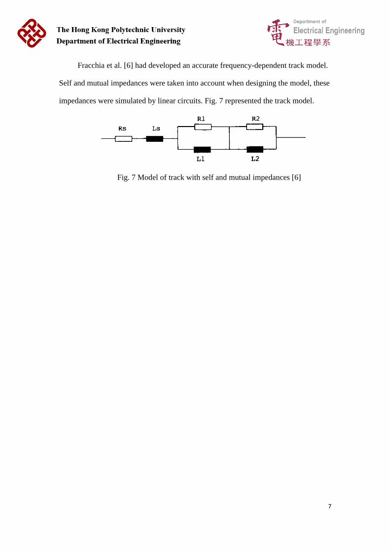
Fracchia et al. [6] had developed an accurate frequency-dependent track model.
Self and mutual impedances were taken into account when designing the model, these
impedances were simulated by linear circuits. Fig. 7 represented the track model.
Fig. 7 Model of track with self and mutual impedances [6]

8
Chapter 4 Methodology
The project is started by developing models for an electric railway system. The
models are later be used to simulate different scenarios Therefore, the models are
developed in detailed so that the results obtained will be helpful in analyzing the
electric railway system. Fig. 8 shows the overview of the proposed electric railway
system with a system block diagram. Description will be given on each component in
the following section.
Fig. 8 System block diagram of the DC transit system
4.1 MATLAB® Simulink
MATLAB® can provide high-performance technical computing power to the
users, a large variety of functions can be programmed and visualized by writing codes
with high-level language.
Simulink is a useful tool under the MATLAB® family. It can model, simulate
and analyze different systems. A number of blocks such as single-/three- phase power
supply and oscilloscope are included. A system can be easily built by dragging the
blocks from the library. It can also support linear and nonlinear system under
continuous or discrete time mode. As a result, Simulink a powerful tool and it is
selected for the development of models and simulations of this project.

9
4.2 Overview of the system
Fig. 9 Overview of the system

10
4.3 Power Supply
The whole electric railway system is powered by a three-phase power source.
Instead of using three separate voltage sources, the Three-Phase Source block in the
Simulink Library is selected to implement a balanced three-phase voltage source with
an internal R-L impedance. It is easier to manage the internal connection of the three
voltage sources. These sources can either be connected to an internal floating neutral,
a neutral connection which is made accessible through a fourth terminal or an
internally grounded neutral.
Fig. 10 Three-Phase Source block
In this project, the Three-Phase Source block is providing 33,000V for the
railway system which is the common voltage supplied to the Hong Kong MTR
Corporation. The 33kV voltage is further stepped down and rectified to suitable DC
voltage level later. The detail parameter of the block is showed in Fig. 11. Both the
internal source resistance and inductance are using the default value. The voltage will
be transmitted to the railway system’s substation through underground cable.

11
Fig.11 Block Parameter (Three-Phase Source)
95mm2 single core armoured copper cable is used for the transmission per phase
and from the typical technical data of a cable manufacturer – Nexans [7], the
resistance, inductance and capacitance are 0.2470Ω/km, 0.401mH/km and
0.324μF/km respectively. For easy calculation, it is assumed that the distance between
the power source and substation is 5km. Since the distance is less than 80km, the lines
can be modelled as short transmission lines where the resistance and inductance are
lumped and the capacitance an admittance are ignored.
Resistance Inductance Capacitance
Cable length: 5km 1.235 Ω 2.02 mH 0 F
Table 1 Parameters of the power cables

12
Fig. 12 Short transmission line model
4.4 Substation
The substation is modelled as three-phase full wave rectifier to convert the AC
voltage to DC voltage. The rectifier will have six diodes in principal. Diodes with odd
number are switched on when phase voltage are positive. On the other hand, the rest
of the diodes are switched on when the phase voltages are negative. 1500V will be
adopted as the output voltage because it is a commonly adopted voltage level in some
of the lines in the Hong Kong MTR Corporation, the voltage will be transmitted
through the overhead catenary.
There are two types of rectifier commonly found in the power transmission
system, namely the Six-pulse and Twelve-pulse rectifier. The Twelve-pulse rectifier is
a combination of two separate sets of Six-pulse rectifier, they can be either connected
in series or in parallel depending on the system. In order to determine which type of
rectifier should be used, simulation on each type of rectifier is carried out and the
decision is based on the results.
4.4.1 Six-pulse rectifier
In this simulation, the normal three-phase AC voltage source, with a difference
of 120 degree between each other phases, is being rectified by 6 diodes. A 50Ω

13
resistor and 300mH inductor are used to mimic as the load. The measurement scope
on the right-hand side will be used to log both the voltage and current of input and
output. The circuit configuration is shown below.
Fig. 13 Six-pulse rectifier configuration
With the aid of the pulse generator in the Simulink library, the pulse for
controlling the thyristors can be easily generated. Since there is only one output port
in the pulse generator block, so it is necessary to include a “Demux” to separate the
six pulses for each of the thyristor. The output signals are connected to the
corresponding thyristor based on the firing sequence. The firing angles of the
thyristors are 30 degrees.
Fig. 14 Order of commutation

14
The average DC voltage can be calculated with the equation:
𝑉𝐷𝐶 =1
𝜋/3∫ �̂�𝐿𝐿 cos 𝜔𝑡 𝑑(𝜔𝑡)
𝜋/6
𝜋/−6
… … … … … … … … … … … 𝐸𝑞. 1
, where �̂�𝐿𝐿 is the peak value of the line – line ac input value. After the
integration, the relationship between the input and output voltage is
𝑉𝐷𝐶 = 3√2
𝜋𝑉𝐿𝐿 … … … … … … … … … … … … … … … … … … . . 𝐸𝑞. 2
With a finite delay angle 𝛼 , the equation becomes:
𝑉𝐷𝐶 = 3√2
𝜋cos 𝛼 𝑉𝐿𝐿 … … … … … … … … … … … … … … … … . 𝐸𝑞. 3
Since the delay angle is set to 30 degrees and the dc output voltage is 750V,
therefore, the required secondary line – line voltage is 1282V. After the simulation,
the resulted waveforms are presented as followed, showing the input voltage, input
current, DC voltage and DC current.
Fig. 15 Simulation result for Six-pulse rectifier
The Powergui Fast Fourier transform (FFT) Analysis Tool is also used to
investigate the harmonic performance of the waveform. After the simulation, the Total

15
Harmonic Distortion (THD) is 24.36%. From Fig.16, it can be observed that the
magnitudes in the 5th order is the highest among the different order of harmonic in the
circuit. Since it is a negative sequence component, it will act against the direction of
rotation in the induction motors and in this way, it will cause torque pulsations and
shaft torsional vibration problems which both are not the desired result.
Fig. 16 FFT Analysis for Six-pulse rectifier
4.4.2 Twelve-pulse rectifier
In order to achieve a proper operation, there should have a 30 degrees difference
in voltage between the two six-pulse rectifiers. This can be tackled by connecting the
secondary sides in wye and delta respectively. The circuit configuration is shown in
Fig. 17. Since the two sets of rectifiers are connecting in series, each set is only
required to rectify 750V. By Eq. 3, the nominal line-line voltage for each secondary
side is 641V.

16
Fig. 17 Twelve-pulse rectifier configuration
From the simulation result, it can be observed that the THD is much better than
that of the six-pulse rectifier. The THD for the Twelve-pulse rectifier is 3.80% and the
input current only contains the 11th and 13th harmonic. Although there is still an 11th
harmonic order, it has a magnitude which is around 2.25% of the fundamental current.
The value is lower than that of the Six-pulse rectifier simulation which is close to 7%,
therefore, the effect on the torque pulsation and shaft torsional vibration can be
reduced.

17
Fig. 18 Simulation result for Twelve-pulse rectifier
Fig. 19 FFT Analysis for Twelve-pulse rectifier
From the two simulations, it is obvious that the system with more pulses is more
effective in reducing the Total Harmonic Distortion and the side-effect like torque
pulsation and shaft torsional vibration. Besides, the DC voltage ripples are also

18
decreased with the Twelve-pulse rectifier, so a DC power with better quality can be
transmitted to the load. Therefore, the Twelve-pulse rectifier is adopted as the model
of the substation.
4.5 Overhead catenary and running rails
4.5.1 Overhead catenary
The overhead catenary has been adopted in a worldwide scale and it also has a
wide range of operating voltages. The system consists of several components like the
messenger wire, the aluminum conductor profile and supporting devices. Mak[8] has
summarized the characteristics of the conductor profile that was adopted by the Hong
Kong MTR Corporation, some useful data is listed below:
Nominal Cross sectional area 2214mm2
Maximum Resistance at 20oC 0.0149Ω/km
Table 2 Conductor profile
If the assumed distance between the train and the substation is 5km, than the
resistance of the contact wire is 0.0745Ω. As for the inductance of the contact wire, it
is defined as the ratio of the total flux linkage to the current.
Inductance (L) =λ
𝐼… … … … … … … … … … … … … … . . Eq. 4
The magnetic field B of a straight current-carrying wire is defined as:
B =𝜇𝑜𝐼
2𝜋𝑟… … … … … … … … … … … … … … … … … … . … . 𝐸𝑞. 5
where 𝜇𝑜: Permeability of free space (4𝜋 x10-7 T m/A)
I: Current
r: Distance from the wire

19
For a length θ, the total flux linkage is
λ = ∫ ∫ 𝐵𝑑𝑟𝑑𝑧 = ∫ ∫𝜇𝑜𝐼
2𝜋𝑟𝑑𝑟𝑑𝑧 =
𝜇𝑜𝐼𝜃
2𝜋𝑙𝑛
𝑏
𝑎… … . 𝐸𝑞. 6
𝑏
𝑎
𝜃
0
𝑏
𝑎
𝜃
0
where b: Radius of the profile
a: Distance between the centre and the copper conductors
The inductance per unit length is:
𝐿
𝜃=
𝜇𝑜
2𝜋𝑙𝑛
𝑏
𝑎… … … … … … … … … … … … … … … 𝐸𝑞. 7
According to Wang and Wang [9], they suggested that the difference between
the inductance at 1 Hz and 105 Hz is approximately equal to internal inductance at DC
voltage and the inductance is given by:
L = 1.024𝜇𝑜
8𝜋[1 − 3𝑆2
1 − 𝑆2−
4𝑆4ln (𝑆)
(1 − 𝑆2)2] … … … … … … … . . 𝐸𝑞. 8
where S is the ratio of inner to outer radius.
Since it is assumed that the contact wire is a solid conductor, therefore S equals
to zero as the inner radius is zero. As a result, the inductance per unit length becomes
0.0512μH/m and the final inductance is 256μH.
Fig. 20 Parameters for 5-km line
20
4.5.2 Running rails
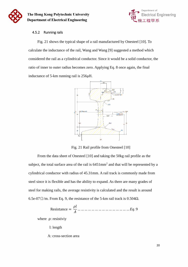
Fig. 21 shows the typical shape of a rail manufactured by Onesteel [10]. To
calculate the inductance of the rail, Wang and Wang [9] suggested a method which
considered the rail as a cylindrical conductor. Since it would be a solid conductor, the
ratio of inner to outer radius becomes zero. Applying Eq. 8 once again, the final
inductance of 5-km running rail is 256μH.
Fig. 21 Rail profile from Onesteel [10]
From the data sheet of Onesteel [10] and taking the 50kg rail profile as the
subject, the total surface area of the rail is 6451mm2 and that will be represented by a
cylindrical conductor with radius of 45.31mm. A rail track is commonly made from
steel since it is flexible and has the ability to expand. As there are many grades of
steel for making rails, the average resistivity is calculated and the result is around
6.5e-07Ω/m. From Eq. 9, the resistance of the 5-km rail track is 0.504Ω.
Resistance = 𝜌𝑙
𝐴… … … … … … … … … … … … … … … 𝐸𝑞. 9
where ρ: resistiviy
l: length
A: cross-section area

21
Fig. 22 Circuit connection (Up to inverter)
Fig. 23 Running rail model
Since the running rails are represented by two cylindrical conductors and they
are carrying the return current, therefore, there should be a certain amount of
capacitance between the two rails. The standard gauge is 1435mm which is set by
Union internationale des chemins de fer[11]. Eq. 10 is used to calculate the
capacitance between two conductors per unit length. The resulted capacitance is
8.05e-12 F/m.

22
C =𝜋휀𝑜
𝑙𝑛𝑑𝑟
… … … … … … … … … … … … … . . 𝐸𝑞. 10
where 휀𝑜: Permittivity of free space (8.85e-12)
d: Distance between two conductors
r: Radius of a conductor
After a quick simulation of the circuit, it is found that, under the current
connection of the components, there are many ripples located in the input voltage
waveform of the inverter as shown in Fig. 24. Therefore, it is necessary to install a
DC-link capacitor between the overhead catenary and the running rails.
Salcone and Bond [12] suggested formulas for calculating the capacitance
and they are presented as followed:
∆𝑉0.5𝑡 = 0.2𝑉𝑝−𝑝 … … … … … … … … … … … … … . . 𝐸𝑞. 11
C =𝑉𝐵𝑢𝑠
(32 ∗ 𝐿 ∗ ∆𝑉0.5𝑡 ∗ 𝑓𝑟𝑒𝑞2)… … … … … … … … … . 𝐸𝑞. 12
From the measuring scope, the peak - peak value of the rectified DC voltage
is measured as around 5200V. Using Eq. 8, Eq. 11 and Eq. 12, the required
capacitance to reduce the ripple is around 310 mF. From Fig. 25, it can be observed
that the voltage waveform is smoother after the installation of the capacitor.

23
Fig. 24 Input voltage waveform at the inverter
Fig. 25 Input voltage waveform at the inverter with a capacitor

24
4.6 Inverter
The inverter is used to convert the supplying DC power to AC power and feed
the AC traction motor later. Six power switching devices are required to build the
inverter and those six devices are represented by using the Universal Bridge for easy
configuration. IGBTs are becoming more common for high voltage and high power
level. For low voltage or low power application, MOSFETs are much more suitable.
Therefore, for this project, the IGBTs are adopted.
Fig. 26 PWM Generator (2-Level) block
The signal for controlling the IGBTs are generated by the PWM Generation (2-
Level) block. The frequency is set as 2000 Hz. The block can generate a symmetrical
or asymmetrical carrier signal in terms of the triangle wave. The input, which is the
reference signal, is then compared with the carrier signal. When the reference signal is
greater than the carrier, the pulse for the upper switching device is high and the pulse
or the lower device is low.
Since, under normal case, the block required the reference signal for the pulse
generation, therefore, a three-phase sine wave generator block is connected to the
block. As a result, the pulse-width modulated waveform is generated by comparing
the amplitude of the control and carrier signals. When the control signal, i.e. the sine
wave, has a higher amplitude, the output voltage will be half of the input DC voltage
(+𝑉𝐷𝐶/2). Otherwise, the output voltage will become −𝑉𝐷𝐶/2. Each phase of the sine
wave will be compared with the carrier signal, the line voltage can then be obtained
by subtracting any two voltage waveforms.

25
For this project, since we want to control the speed of the induction motor, so
the three-phase sine wave generator is not used, instead, we will obtain the
information like the flux or the transformed current from the induction motor, and
then by mathematical formula we can obtain three sine-wave-like waveforms. These
waveforms is later transmitted to the input port of the PWM Generator (2-level) for
the firing of the IGBTs. The details of obtaining the new waveform will be further
discussed in following session.
Fig. 27 Inverter configuration
Fig. 28 Normal output waveforms of the inverter (Phase-A voltage, Phase-B
voltage and Line A-B voltage)

26
4.7 Traction motor
The model for traction motor will be built with reference to the dynamic of the
rotor and stator. In order to do so, the input three-phase components have to first go
through two transformations, namely the Clarke and the Park Transforms, and the
input voltage or current will be represented in the way of two-phase orthogonal axis.
The obtained components can then be used to calculate the torque and the rotational
speed of the motor.
Clarke Transformation is used to convert the three-phase quantities into a two-
phase quadrature quantities which is represented in the α-β axis. This representation is
called the two-axis orthogonal stationary reference frame. The transformation can be
done by using the following matrix equation and Fig. 30 shows the connection inside
the Clarke Transformation block.
Fig. 29 Clarke Transformation matrix
Fig. 30 Connection inside the Clarke Transformation Block
27
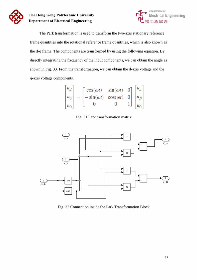
The Park transformation is used to transform the two-axis stationary reference
frame quantities into the rotational reference frame quantities, which is also known as
the d-q frame. The components are transformed by using the following equation. By
directly integrating the frequency of the input components, we can obtain the angle as
shown in Fig. 33. From the transformation, we can obtain the d-axis voltage and the
q-axis voltage components.
Fig. 31 Park transformation matrix
Fig. 32 Connection inside the Park Transformation Block

28
Fig. 33 Connection between the angle block and Park transformation block
The d- and q- axis stator and rotor voltage (𝑉𝑑𝑠, 𝑉𝑞𝑠, 𝑉𝑑𝑟, 𝑉𝑞𝑟) are related to the
stator resistance 𝑅𝑠, d- and q- axis stator and rotor current (𝑖𝑑𝑠, 𝑖𝑞𝑠, 𝑖𝑑𝑟, 𝑖𝑞𝑟), flux
linkages (𝜆𝑑𝑠, 𝜆𝑞𝑠, 𝜆𝑑𝑟, 𝜆𝑞𝑟), angular velocity of the frame and the rotor (𝜔𝑒 & 𝜔𝑟).
Their relationship can be expressed in the following equations [13]. The rotor
voltages are set to be zero because it is assumed the induction motor is a squirrel-cage
type machine. The parameters of the above components are listed in the following
table.
Table 3 Parameters of the induction motor
Value
Stator resistance 0.087 Ω
Rotor resistance 0.228 Ω
Magnetizing inductance 34.7 mH
Stator and Rotor inductance 35.5 mH
Stator and Rotor leakage
inductances
0.8 mH
Moment of inertia 4.179 kg m2

29
V𝑑𝑠 = 𝑅𝑠𝑖𝑑𝑠 +𝑑𝜆𝑑𝑠
𝑑𝑡− 𝜔𝑒𝜆𝑞𝑠 … … … … … … … … … 𝐸𝑞. 13
V𝑞𝑠 = 𝑅𝑠𝑖𝑞𝑠 +𝑑𝜆𝑞𝑠
𝑑𝑡+ 𝜔𝑒𝜆𝑑𝑠 … … … … … … … … … 𝐸𝑞. 14
V𝑑𝑟 = 𝑅𝑟𝑖𝑑𝑟 +𝑑𝜆𝑑𝑟
𝑑𝑡− (𝜔𝑒 − 𝜔𝑟)𝜆𝑞𝑟 = 0 … … … … … … … … … 𝐸𝑞. 15
V𝑞𝑟 = 𝑅𝑟𝑖𝑞𝑟 +𝑑𝜆𝑞𝑟
𝑑𝑡+ (𝜔𝑒 − 𝜔𝑟)𝜆𝑑𝑟 = 0 … … … … … … … … … 𝐸𝑞. 16
The flux linkages have the relationship between the stator and rotor inductance,
and the d- and q-axis stator and rotor current. 𝐿𝑚 is the magnetizing inductance and
it is the difference between the stator / rotor inductances and the stator / rotor leakage
inductances.
𝜆𝑑𝑠 = 𝐿𝑠𝑖𝑑𝑠 + 𝐿𝑚𝑖𝑑𝑟 … … … … … … … … … 𝐸𝑞. 17
𝜆𝑞𝑠 = 𝐿𝑠𝑖𝑞𝑠 + 𝐿𝑚𝑖𝑞𝑟 … … … … … … … … … 𝐸𝑞. 18
𝜆𝑑𝑟 = 𝐿𝑚𝑖𝑑𝑠 + 𝐿𝑟𝑖𝑑𝑟 … … … … … … … … … 𝐸𝑞. 19
𝜆𝑞𝑟 = 𝐿𝑚𝑖𝑞𝑠 + 𝐿𝑟𝑖𝑞𝑟 … … … … … … … … … 𝐸𝑞. 20
By changing the subjects and substituting Eq. 17 – 20 into Eq. 13 – 16, one can
obtain the differential equations for the flux linkages (𝜆𝑑𝑠, 𝜆𝑞𝑠, 𝜆𝑑𝑟, 𝜆𝑞𝑟). Taking the
d-axis stator flux linkage as an example, the differential equation is shown in Eq. 21.
𝑑𝜆𝑑𝑠
𝑑𝑡= V𝑑𝑠 −
𝑅𝑠𝐿𝑟
𝐿𝑠𝐿𝑟 − 𝐿𝑚2 𝜆𝑑𝑠 +
𝑅𝑠𝐿𝑚
𝐿𝑠𝐿𝑟 − 𝐿𝑚2 𝜆𝑑𝑟 + 𝜔𝑒𝜆𝑞𝑠 … … … … … 𝐸𝑞. 21
The models can be built to obtain the four flux linkage values based on the differential
equations. Fig.34 shows the general connections inside the block and Fig. 35 shows
the connection for Eq. 21.

30
Fig. 34 General connection inside the block
Fig. 35 Connection for Eq. 21
By changing subjects as 𝑖𝑑𝑠, 𝑖𝑞𝑠, 𝑖𝑑𝑟 𝑎𝑛𝑑 𝑖𝑞𝑟 for Eq. 17 – 20, one should obtain
an equation like Eq. 22 during the substitutions for Eq. 13 – 16. The four current
values can be obtained by direct substitutions and Fig. 36 shows the connection for
calculating 𝑖𝑑𝑠, 𝑖𝑞𝑠, 𝑖𝑑𝑟 𝑎𝑛𝑑 𝑖𝑞𝑟.
𝑖𝑑𝑠 = 𝐿𝑟
𝐿𝑠𝐿𝑟 − 𝐿𝑚2 𝜆𝑑𝑠 −
𝐿𝑚
𝐿𝑠𝐿𝑟 − 𝐿𝑚2 𝜆𝑑𝑟 … … … … . . 𝐸𝑞. 22

31
Fig. 36 Connections for calculating 𝑖𝑑𝑠, 𝑖𝑞𝑠, 𝑖𝑑𝑟 𝑎𝑛𝑑 𝑖𝑞𝑟
After obtaining the four current value, then the torque can be calculated by
using the following equation:
T = 3
2×
𝑃
2𝐿𝑚 (𝑖𝑑𝑟 𝑖𝑞𝑠 − 𝑖𝑞𝑠 𝑖𝑑𝑠) … … … … … … 𝐸𝑞. 23
, where p is the number of poles of the traction motor and it is assumed that the motor
has four poles. The constant part of Eq. 23 is 0.1041 with the 𝐿𝑚 setting at a value of
34.7 mH.
Fig. 37 Connection for calculating the torque

32
Fig. 38 Torque characteristic curve when load torque is 300Nm
The rotor rotating speed can then be calculated by integrating the difference in
electromagnetic torque and load torque, and the moment of inertia with respect to
time. Eq. 24 shows the calculation of the speed where J is the moment of inertia of the
rotor and 𝑇𝐿 is the load torque. Noted that, as shown in Fig. 39, the calculated
angular velocity has to be fed back to the pervious block for the calculation of the flux
linkages.
𝜔𝑟 =𝑃
2𝐽∫ (𝑇 − 𝑇𝐿) 𝑑𝑡 … … … … … … … … … … 𝐸𝑞. 24
𝑡
0
From Fig.40, we can see that the motor has an oscillation of torque between
9500Nm and -500Nm when the simulation just started. During the oscillation, the
speed of motor increased from zero to around 6000 rpm. Once the torque is stabilized,
the speed of motor is also remained at a stable value.
Fig. 39 Connections between different blocks of the traction motor

33
Fig. 40 Rotor’s angular velocity (Curve in Yellow color)
4.8 PWM signal generation
The PWM signal is generated by using the vector control. This is a control
method that both the magnitude and the phase of current and voltage are regulated. By
using this kind of control method, the motor can be made to perform desirable torque
and speed responses because the current and voltage vectors can be used to determine
the flux magnitude, as well as the torque. Fig. 41 shows the connections of blocks for
generating PWM signal.
Fig. 41 System diagram for generating PWM signal
𝜓𝛼𝑠 = ∫(𝑉𝛼 − 𝑖𝛼𝑅𝑠) 𝑑𝑡 … … … … … . 𝐸𝑞. 25
𝜓𝛽𝑠 = ∫(𝑉𝛽 − 𝑖𝛽𝑅𝑠) 𝑑𝑡 … … … … … . 𝐸𝑞. 26

34
𝜓𝑠 = √𝜓𝛼𝑠2 + 𝜓𝛽𝑠
2 … … … … … . . 𝐸𝑞. 27
𝜌𝑠 = 𝑡𝑎𝑛−1𝜓𝛽𝑠
𝜓𝛼𝑠… … … … … … … . . . 𝐸𝑞. 28
The flux amplitude and angle can be determined by the above equations. The α-
and β-axis current required in Eq. 25 and 26 is determined by using the inverse Park
Transformation. These current is later transformed back to the d-q reference frame
vectors for further comparison.
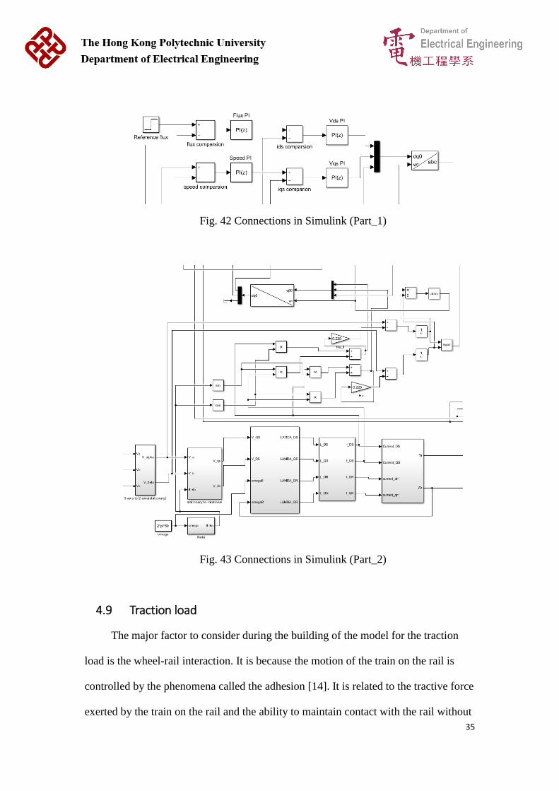
The resulted flux is then passed to the comparison block to be compared with
the reference flux. The reference speed and the motor speed is also compared in the
block. The signals are later passed to the Flux and Speed PI controllers and the output
of these PI controllers are the reference d-axis current and reference q-axis current
respectively. There is another idential block for the comparison of the d- and q-axis
current. The output of these PI controllers are the d- and q-axis stator voltage. The
determination of those P nad I parameters are based on the trial and error. Table 4
shows the desired controller parameters for the four PI controllers in the comparion
blocks.
The resulted d- and q-axis stator voltage are transformed back to the standard
three-phase frame. These voltage signals become the input of the PWM generator
mentioned in Chapter 4.6. Six firing pulses for controlling the Inverter block are
generated.
Proportional (P) Integral (I)
Flux PI controller 0.95 0.09
Speed PI controller 1.02 0.0051
d-axis stator voltage PI controller 1.1 0.13
q-axis stator voltage PI controller 0.97 0.0048
35
Fig. 42 Connections in Simulink (Part_1)
Fig. 43 Connections in Simulink (Part_2)
4.9 Traction load
The major factor to consider during the building of the model for the traction
load is the wheel-rail interaction. It is because the motion of the train on the rail is
controlled by the phenomena called the adhesion [14]. It is related to the tractive force
exerted by the train on the rail and the ability to maintain contact with the rail without
36
any sliding. When the train is able to produce sufficient tractive force, which is also
known as the tractive effort, and the force and torque can successfully overcome the
resistive force applied on the train, then the train can accelerate. The tractive effort
can be calculated as the multiple of the axle load and the coefficient of adhesion as
shown in Eq. 29
𝐹𝑇𝐸 = 𝜇 𝑁 … … … … … … … … … … . 𝐸𝑞. 29
The modelling of the coefficient of adhesion is taken from Polach[15] which has
derived equations from calculating the friction coefficient. Spiryagin et al. [16] agreed
that the models from Polach[15] provide shorter processing time and is “perfectly
suited for a simplified approach”. The corresponding equations are shown below and
some of the parameters are also extracted from Polach[15] to simulate the dry wheel-
rail conditions.
Adhesion coefficient = 2𝛿
𝜋(
휀
1 + 휀2+ arctan 휀) … … … … … … . 𝐸𝑞. 30
δ = 𝛿0[(1 − 𝐴)𝑒−𝐵𝓌 + 𝐴] … … … … … … … … … … . 𝐸𝑞. 31
ε = 1
4
𝐺𝜋𝑎𝑏𝑐11
𝑄𝛿𝑠 … … … … … … … . 𝐸𝑞. 32
,where A = ratio of friction coefficients 𝜇∞
𝜇𝑜
B = coefficient of exponential friction decrease (s/m)
𝛿0 = maximum friction coefficient at zero slip velocity
𝛿∞ = maximum friction coefficient at infinity slip velocity
ε = gradient of the tangential stress
𝓌 = total creep (slip) velocity
Q = wheel load
s = total slip %
a = half-axis of the contact ellipse in x-direction
b = half-axis of the contact ellipse in y-direction
c11 = coefficient from Kalker’s linear theory
G = shear module of steel
37
Value
A 0.4
B 0.6
𝛿0 0.55
Q 200 kN
a 6.16mm
b 9.24mm
c11 3.9339667
G 7.79 x 10¹⁰ N/m2
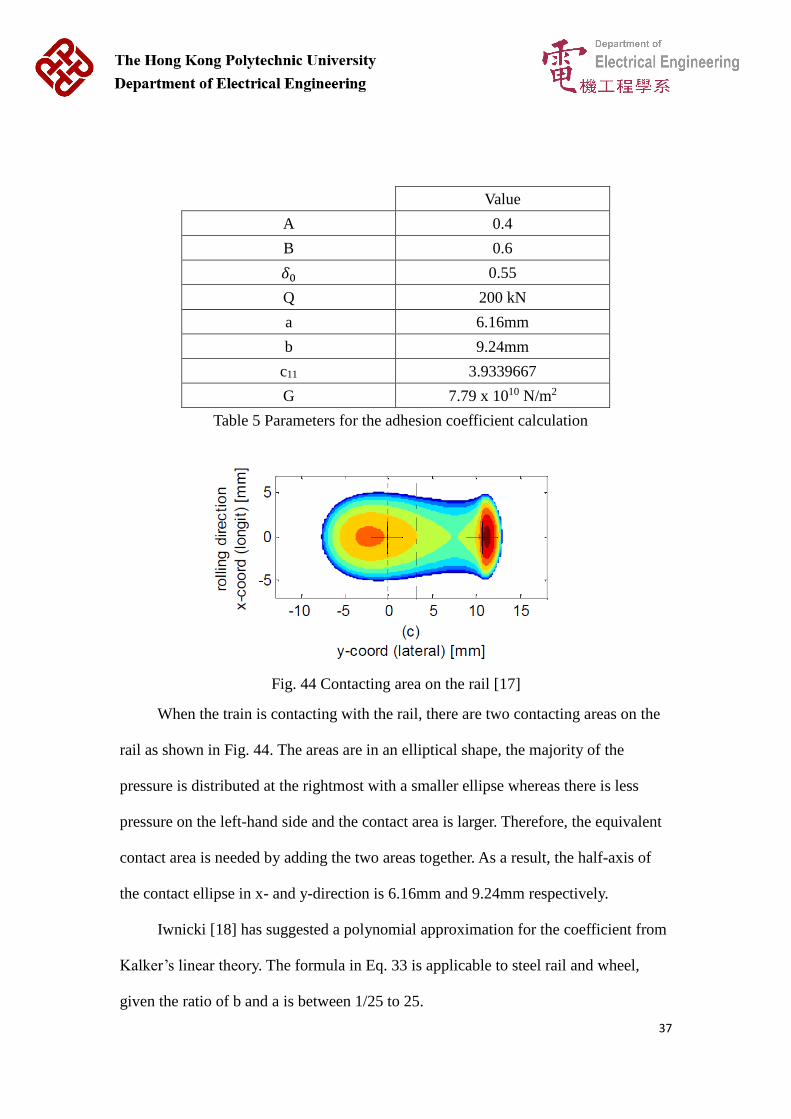
Table 5 Parameters for the adhesion coefficient calculation
Fig. 44 Contacting area on the rail [17]
When the train is contacting with the rail, there are two contacting areas on the
rail as shown in Fig. 44. The areas are in an elliptical shape, the majority of the
pressure is distributed at the rightmost with a smaller ellipse whereas there is less
pressure on the left-hand side and the contact area is larger. Therefore, the equivalent
contact area is needed by adding the two areas together. As a result, the half-axis of
the contact ellipse in x- and y-direction is 6.16mm and 9.24mm respectively.
Iwnicki [18] has suggested a polynomial approximation for the coefficient from
Kalker’s linear theory. The formula in Eq. 33 is applicable to steel rail and wheel,
given the ratio of b and a is between 1/25 to 25.
38
𝑐11 = 3.2893 +0.975
𝑏𝑎
− (0.012
𝑏𝑎
2 ) … … … … … . . 𝐸𝑞. 33
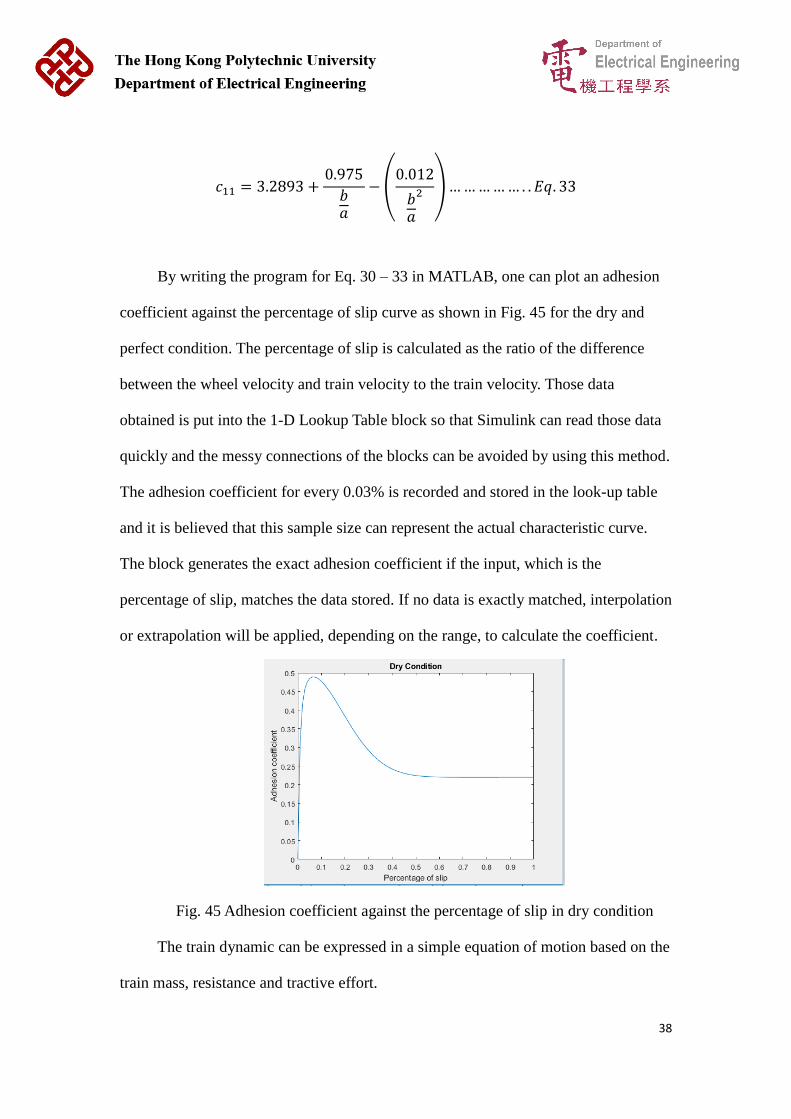
By writing the program for Eq. 30 – 33 in MATLAB, one can plot an adhesion
coefficient against the percentage of slip curve as shown in Fig. 45 for the dry and
perfect condition. The percentage of slip is calculated as the ratio of the difference
between the wheel velocity and train velocity to the train velocity. Those data
obtained is put into the 1-D Lookup Table block so that Simulink can read those data
quickly and the messy connections of the blocks can be avoided by using this method.
The adhesion coefficient for every 0.03% is recorded and stored in the look-up table
and it is believed that this sample size can represent the actual characteristic curve.
The block generates the exact adhesion coefficient if the input, which is the
percentage of slip, matches the data stored. If no data is exactly matched, interpolation
or extrapolation will be applied, depending on the range, to calculate the coefficient.
Fig. 45 Adhesion coefficient against the percentage of slip in dry condition
The train dynamic can be expressed in a simple equation of motion based on the
train mass, resistance and tractive effort.

39
𝐹𝑇𝐸 − 𝑅𝑡𝑜𝑡𝑎𝑙 = 𝑀𝑑𝑣
𝑑𝑡… … … … … 𝐸𝑞. 34
The total resistance consists of two elements, the train rolling resistance and the
gradient resistance. The gradient resistance can be expressed in Mgsinθ. The train
rolling resistance has a general formula
R𝑟 = α + β ∙ v + γ ∙ 𝑣2 … … … … … 𝐸𝑞. 35
The v2-coefficient is used in tunnel condition and since most of the railway lines
in Hong Kong are located inside the tunnel, so this coefficient is taken into account in
this project. Steimel[19] has added a constant of 15 to v2-coefficient to compensate
the head wind in the tunnel and has also provided the practical value for the
α, β and γ.
α β γ
1.0 0.0025 0.0696 ∙𝑛 + 2.7
𝐺
Table 6 Parameter for the train rolling resistance
where n = number of coaches = 8
G = weight force of train = 320 tonnes = 3139 kN
The Eq. 35 is normalized to the train weight force and the resistance force is
given in per kilo-Newton. Therefore, it is necessary to multiply with the train weight
force to obtain the true value for the resistance.
40
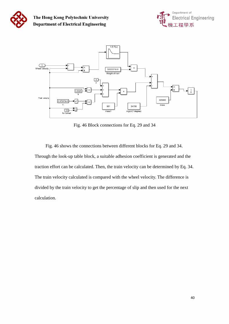
Fig. 46 Block connections for Eq. 29 and 34
Fig. 46 shows the connections between different blocks for Eq. 29 and 34.
Through the look-up table block, a suitable adhesion coefficient is generated and the
traction effort can be calculated. Then, the train velocity can be determined by Eq. 34.
The train velocity calculated is compared with the wheel velocity. The difference is
divided by the train velocity to get the percentage of slip and then used for the next
calculation.
41
Chapter 5 Results
In this chapter, simulation results of the models mentioned in the Chapter 4 will
be presented. Scenarios like the start-up of trains and internal / external faults will
also be included.
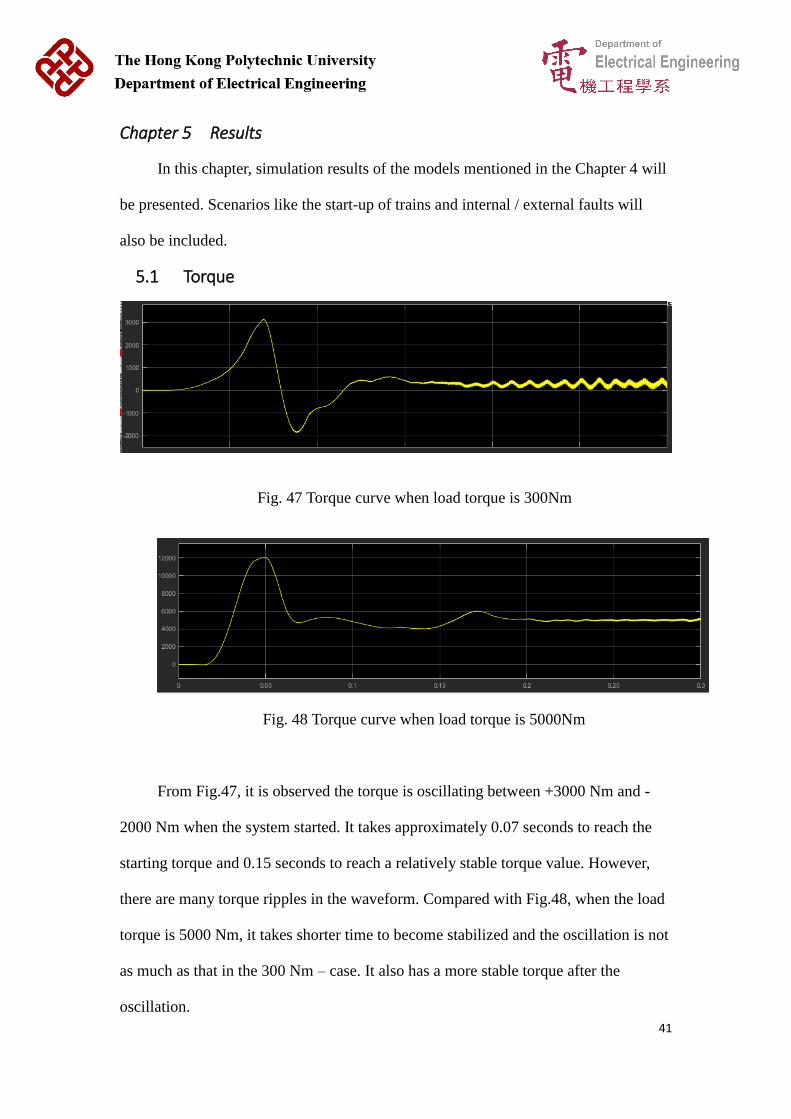
5.1 Torque
Fig. 47 Torque curve when load torque is 300Nm
Fig. 48 Torque curve when load torque is 5000Nm
From Fig.47, it is observed the torque is oscillating between +3000 Nm and -
2000 Nm when the system started. It takes approximately 0.07 seconds to reach the
starting torque and 0.15 seconds to reach a relatively stable torque value. However,
there are many torque ripples in the waveform. Compared with Fig.48, when the load
torque is 5000 Nm, it takes shorter time to become stabilized and the oscillation is not
as much as that in the 300 Nm – case. It also has a more stable torque after the
oscillation.

42
5.2 Wheel and train velocities
Fig. 49 Wheel and train velocities
From Fig. 49, the yellow line represents the wheel speed and the blue line
represent the train speed. It is observed that there is a slight difference in the speed
between the two bodies. This is related to the creep characteristic. It is important to
have the phenomenon because the wheel should be moving faster than the train, such
that the wheel is rotating and delivering sufficient tractive effort to drive the train,
instead of sliding on the rails.
5.3 PI controllers
The Proportional and Integral parameters are determined by trial and error. The
reference flux is 0.56Wb. The wheel velocity are compared with the reference speed.
The reference speed will first ramp to a certain value and hold for a short period of
time, then it will ramp again.
Case 1 Proportional (P) Integral (I)
Flux PI controller 1.4 0.125
Speed PI controller 1.02 0.0051
d-axis stator voltage PI controller 1.1 0.6
q-axis stator voltage PI controller 0.91 0.0034
Table 7 Parameters of PI controllers (Case 1)

43
Fig. 50 Simulation result of Case 1
The curve in yellow is the speed of train and it can be observed that after 0.65
seconds, the speed of train cannot track well so modification of the parameters is
needed.
Case 2 Proportional (P) Integral (I)
Flux PI controller 1 0.1
Speed PI controller 1 0.005
d-axis stator voltage PI controller 1 0.1
q-axis stator voltage PI controller 1 0.005
Table 8 Parameters of PI controllers (Case 2)
Fig. 51 Simulation result of Case 2
After the modification, the response of the train speed becomes better. It takes
around 0.15s to become stabilized. There can be a small adjustment to improve the
performance. Table 8 shows the amendment on the parameters and from Fig. 52, it

44
can be observed that it takes shorter time to become stabilized and the difference
between the reference signal and train speed is acceptable.
Case 3 Proportional (P) Integral (I)
Flux PI controller 0.95 0.09
Speed PI controller 1.02 0.0051
d-axis stator voltage PI controller 1.1 0.13
q-axis stator voltage PI controller 0.97 0.0048
Table 8 Parameters of PI controllers (Case 3)
Fig. 52 Simulation result of Case 3
5.4 Start – up of trains
The following scenarios are simulated:
Trains are starting up at 5.0km away from the substation
Trains are starting up at 0.1km away from the substation
Since the distance between the substation and trains is changed, the resistance
and inductance of the overhead catenary and running rails have to be changed as well
according to Eq. 8 and 9. The DC-link capacitance also have to amend with respect to
the ripple in the rectified DC voltage waveforms. The simulation results are as
followed:

45
Fig. 53 Simulation result of trains starting up at 5.0km away from the substation
Fig. 54 Simulation result of trains starting up at 0.1km away from the substation
It can be observed that if the trains are starting up far away from the
substation, the peak current at the initial time is smaller and there is no oscillation
before reaching the stable level. When the trains are starting at a closer distance to the
substation, there will be a higher overshoot in the current waveform and it needs some
oscillations before reaching a stable level. Therefore, the setting of the circuit breakers
should be carefully designed.
5.5 Internal / external faults
Simulation results of faults are presented in this section. The faults can be
occurred at places like the transmission line or at the train’s internal component. The
simulations are also carried out when the trains are at different locations, like 0.1km
and 5.0km away from the substation. The fault signal is generated by using the break
block as shown in Fig. 55 and 56. The type of fault happened depends on what is the
output port connected to.

46
Fig. 55 Breaker block
Fig. 56 Parameters of the breaker block
The external phase-to-ground fault is simulated in the project and the fault is
located at the overhead catenary. The internal switching time setting is selected to be
0.1s, when the time is reached, the breaker will be switched on. Different breaker
resistances will be also set to mimic the fault resistances.
Fig. 57 Block connection
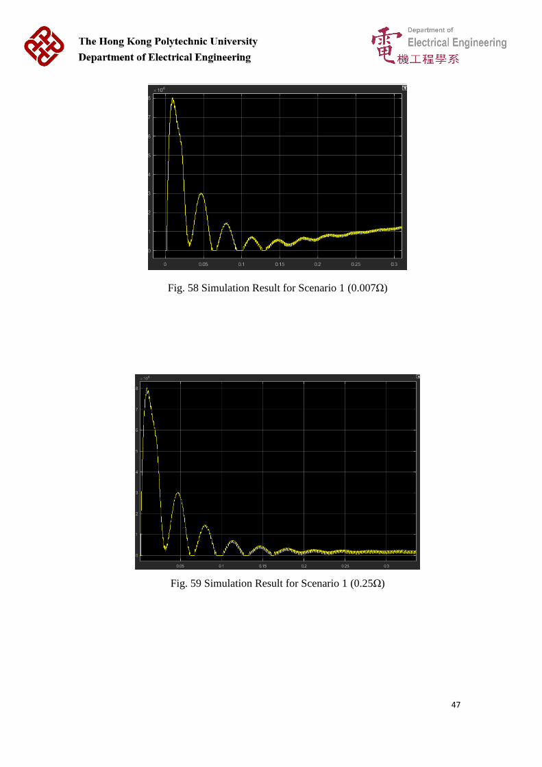
47
Fig. 58 Simulation Result for Scenario 1 (0.007Ω)
Fig. 59 Simulation Result for Scenario 1 (0.25Ω)

48
Fig. 60 Comparison between two fault resistances (scenario 1)
Scenario 1 simulates the phase-to-ground fault happened at the overhead
catenary when the train is 0.1 km away from the substation. It can be observed that
after the fault is happened at 0.1s, the current reached a higher fault value at 0.3s
which is represented in the blue in Fig. 60, when the fault resistance is 0.007Ω. The
red curve in Fig. 60 shows the current response when the fault resistance is 0.25Ω.
The fault current at 0.3s are 11820A and 2241A respectively.

49
Fig. 61 Simulation Result for Scenario 2 (0.007Ω)
Fig. 62 Simulation Result for Scenario 2 (0.25Ω)
50
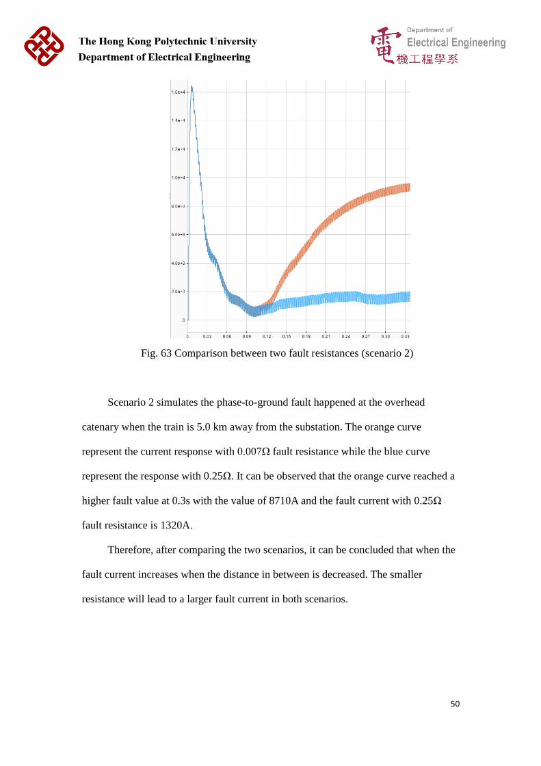
Fig. 63 Comparison between two fault resistances (scenario 2)
Scenario 2 simulates the phase-to-ground fault happened at the overhead
catenary when the train is 5.0 km away from the substation. The orange curve
represent the current response with 0.007Ω fault resistance while the blue curve
represent the response with 0.25Ω. It can be observed that the orange curve reached a
higher fault value at 0.3s with the value of 8710A and the fault current with 0.25Ω
fault resistance is 1320A.
Therefore, after comparing the two scenarios, it can be concluded that when the
fault current increases when the distance in between is decreased. The smaller
resistance will lead to a larger fault current in both scenarios.
51
Chapter 6 Conclusion and future development
6.1 Conclusion
In this project, MATLAB Simulink has provided a good environment for the
development of models and the simulations. The models of different system
components have beeen successfully built, detail descriptions on how to develop each
models are provided so as to allow the readers to understand the procedures.
Furthermore, when building the models, different parameters are put into
consideration, for instance, the selection of Six-pulse rectifier and Twelve-pulse
rectifier based on the Total Harmonic Distortion, the dynamic of stator and rotor when
build the traction motor model and the adhesion coefficient in the traction load model.
Simulations are carried out to observe the torque response, the wheel-train
speed, setting of PI controllers, start-up of trains and external faults in this report. The
simulation results show that when the load torque is low, the motor takes longer time
to become stabilized. From the wheel-train speed simulation, it is found that there is a
small difference between the speed of wheel and train because of the slip. The
adhesion ensures that the wheel is rotating to give tractive effort to drive the train
instead of sliding on the rails. The start-up of trains’ simulation indicates that when
the train is starting at a closer distance to the substation, the peak current value is
higher and vice versa. In the external fault analysis, the fault is set at the overhead
catenary with different fault resistance values, it is found that a shorter distance in
between and a smaller fault resistance leads to a higher magnitude in the fault current.
To conclude, this project has successfully built the detail models for different
components in the electric railway system and simulations are carried out to
demonstrate the effect of incidents to the system.
52
6.2 Future development
For the future development, the models built can be further co-simulated with
other specific software. Simulink is very friendly for the development of data
exchange connections with multibody packages. It makes the process of simulating
train dynamic behavior under different operational conditions relatively easily.
More mechanical system component can also be considered and included in the
traction load model, such as the bogies and the suspension. In this way, the simulation
results can be able to analyze and optimize the vehicle dynamic behavior for the
wheel – rail interface. The more realistic and comprehensive results can also be used
for the railway wheel – rail wear profile prediction and the accumulated rolling
contact fatigue damage determination through co-simulating with other software as
mentioned above.

53
Chapter 7 Reference
[1] International Union of Railways, A global vision for railway development, 2015.
[Online]. Available: http://uic.org/IMG/pdf/global_vision_for_railway_development.
pdf [Accessed Sept. 18, 2017].
[2] D. M. Z. Islam and M. Blinge, “The future of European rail freight transport and
logistics,” European Transport Research Review, vol. 9, no. 1, pp. 11, Feb 2017.
[3] The Royal Academy of Engineering Sciences, “Electricity production in
Sweden,” Sweden: The Royal Academy of Engineering Sciences, 2016.
[4] M. X. Li, J. H. He, Z. Q. Bo, H. T. Yip, L. Yu and A. Klimek, “Simulation and
Algorithm Development of Protection Scheme in DC Traction System,” 2009 IEEE
Bucharest PowerTech, pp. 1-6, Jun 2009.
[5] R. J. Hill and J. Lamacq, “Railway traction vehicle electromechanical simulation
using SIMULINK,” Computers in Railway, vol. 2, no. 96, pp. 157-166.
[6] M. Fracchia, R. J. Hill, P. Pozzobon and G. Sciutto, “Accurate track modeling for
fault current studies on third-rail metro railways,” Railroad Conference 1994
Proceedings of the 1994 ASME/IEEE Joint (in conjunction with Area 1994 Annual
Technical Conference), pp. 97-102, 1994.
[7] Nexans, 6-36kV Medium Voltage Underground Power Cables, 2010. [Online].
Available:http://www.nexans.co.uk/UK/files/Underground%20Power%20Cables%20
Catalogue%2003-2010.pdf [Accessed Dec. 26, 2017].
[8] M.K. Mak, “Adoption of Overhead Rigid Conductor Rail System in MTR
Extensions,” Journal of International Council on Electrical Engineering, vol. 2, no. 4,
pp 463-466, Sep 2014.
54
[9] Y.J. Wang and J.H. Wang, “Modeling of Frequency-Dependent Impedance of the
Third Rail Used in Traction Power Systems,” IEEE Transactions on power delivery,
vol.15, no. 2, pp. 750-755, Apr 2000.
[10] Onesteel, Rail Track Material, 2013. [Online]. Available: https:// www.
libertyonesteel.com/media/2407/onesteel-rail-track-material-catalogue.pdf [Accessed
Dec.29, 2017].
[11] Union internationale des chemins de fer, High Speed Rail History, 2015.
[Online]. Available: https://uic.org/High-Speed-History [Accessed Dec. 30, 2017].
[12] M. Salcone and J. Bond, “Selecting Film Bus Link Capacitors For High
Performance Inverter Applications,” 2009 IEEE International Electric Machines and
Drives Conference, pp. 1692-1699, May 2009.
[13] S. Shah, A. Rashid and M. Bhatti, “Direct Quadrate (D-Q) Modeling of 3-Phase
Induction Motor Using MatLab / Simulink,” Canadian Journal on Electrical and
Electronics Engineering, vol. 3, no. 5, pp. 237-243, May 2012.
[14] S. Senini, F. Flinders and W. Oghanna, “Dynamic simulation of wheel-rail
interaction for locomotive traction studies,” Proceedings of the 1993 IEEE/ASME
Joint Railroad Conference, pp. 27-34, Apr 1993.
[15] O. Polach, “Creep forces in simulations of traction vehicles running on adhesion
limit,” Wear, vol. 258, no. 7, pp. 992-1000, Mar 2004.
[16] M. Spiryagin, P. Wolfs, C. Cole, V. Spiryagin, Y. Q. Sun and T. McSweeney,
Design and Simulation of Heavy Haul Locomotive and Trains. New York: CRC Press,
2017, p.240.
[17] R. Popovici, “Friction inWheel - Rail Contacts,” Ph.D. thesis, Department of
Engineering Technology, University of Twente, Netherlands, 2010. [Online].
Available: https://www.utwente.nl/en/et/ms3/research-chairs/stt/research/publications/
phd-theses/Thesis_Popovici.pdf
[18] S. Iwnicki, Handbook of Railway Vehicle Dynamics. New York: CRC Press,
2006.

55
[19] A. Steimel, Electric Traction – Motive Power and Energy Supply Basics and
Practical Experience 2nd edition. München: Deutscher Industrieverlag, 2014, pp.38.