Project 4 Financials (Excel) - Personal World Wide Web...

of 15

Project 4 – Financials (Excel)

Project Objective To offer an introduction to building spreadsheets, creating charts, and entering functions.

Part 1 - Financial Projections

One of the most important aspects of analyzing the feasibility and profitability of a new business is creating financial statements, projecting cash flows, and keeping track of information. For the purpose of this part, you will be creating a 3-year income statement for two different business opportunities: 1) operating a plant in Location A or 2) operating a plant in Location B. This will allow you to assess the profitability of your new endeavor after a few years of commerce and therefore make an informed decision as to which opportunity you should pursue. You will begin by creating the 3-year income statement for Location A.

Income Projection for Location A

Figure 1: Location A Financials worksheet

of 15

Initial Layout:

Figure 2: Initial Data for Location A

Refer to figures 1 and 2 for the following tasks.

1. Start Microsoft Excel (instructions for Microsoft Excel 2010). You will notice you have three worksheets in your new Excel workbook.

2. In Sheet1, enter the following text in cell B3: Location A’s Projected Income Statement. 3. Select the cells B3:E3 and click on the Merge & Center button in the Home tab. 4. In cell A5, enter the text: Revenues. 5. Enter the text in column A (cells A5:A37) as shown in Figure 2, including the text in the

second table at the bottom (The Financial Summary Table). Cell A37 contains the text: * pre tax.

of 15

6. In cell C31, enter the text: FINANCIAL SUMMARY. 7. In cell B4, enter the text: YEAR. Enter the 3 years shown across that row. 8. Enter numbers for your Revenues, Cost of Sales, and Operating Expenses for the next

years. Use the numbers provided in the screenshot above. Do not enter the Total amounts. 9. Use the SUM function to calculate all of the totals for the Revenues, Cost of Sales, and

Operating Expenses for cells C10, D10, E10, C16, D16, E16, C26, D26, and E26. 10. Enter a formula to calculate the Gross Profit for the three years (cells C18:E18). For the first

year, you would enter the following formula in cell C18: =C10-C16. 11. Use a formula to calculate the Net Revenue/Loss for all three years (cells C28:E28). For the

first year, you would enter the following formula in cell C28: =C18-C26. 12. Format all of the values with $ and no cents. Under the Home tab, click the currency icon

(dollar sign on Windows and dollar bill with coins on Mac), and click the Decrease Decimal button (.00 .0) twice.

13. Use the shading, border, and font color features to make your income statement look like the one in Figure 1 above. The colors and widths do not need to be exact, but every feature must be utilized as per the specifications implied in the screenshot.

14. In Cell C1, enter your company’s name. Then merge & center it in cells C1:E1. 15. Adjust the column widths as necessary to display all cell contents.

The Financial Summary Table:

16. Use cell references in the Financial Summary Table to display the numbers for Revenues, Cost of Sales, Gross Profit, and Operating Expenses from the Income Statement above in the worksheet. Do not simply type the numbers in or your sheet will not work. For cell C32, enter = and then click on cell C10.

17. Merge & center the text Financial Summary in cells C31:E31. 18. Format the table similar to the table shown in Figure 1. If you would like, you can use the

Cell Styles option in the Home tab.

The 3-Year Financial Statistics Table:

19. Enter the text for Average, Largest, and Smallest Net Revenue/Loss in cells G32:G34. 20. For cell K32, use the Average function to calculate the average net revenue/loss by using

cells C28:E28. 21. For cell K33, use the Max function to calculate the largest net revenue/loss by using cells

C28:E28. 22. For cell K34, use the Min function to calculate the smallest net revenue/loss by using cells

C28:E28. 23. Merge & center the text 3-Year Financial Statistics in cells G31:K31. 24. Format the table using shading, borders, and font colors. Again, make them similar, but

they do not have to be exact.

The Chart

25. Select all of the Revenues Totals (C10:E10), Cost of Sales Totals (C16:E16), and Operating Expenses Totals (C26:E26) simultaneously by holding down the [Ctrl] (or control) button and selecting the three sets of cells.

26. Select the Insert tab.

of 15

27. Add a chart, by selecting the Line pull-down, and then the Line with Markers option. 28. Define the parameters of the chart:

a. Under the Chart Tools, select the Design tab. b. Click the Select Data option. c. Click the Edit button under the Horizontal (Category) Axis Labels section. Select the

years cells (C4:E4) of your spreadsheet and hit the Enter key. d. Change the name of Series1, Series2, and Series3 to Revenues, Cost of Sales, and

Operating Expenses, respectively, by selecting the Edit button under the Legend Entries (Series) section. Change them by clicking in the area for Series name and selecting the cell containing the label for Revenues. Do this for all three labels.

e. In the Select Data Source window, press the OK button. 29. Under the design tab, expand the Chart Layouts area by clicking on the arrow below the

down arrow. Select Chart Layout 5. 30. Adjust the layout of your chart by selecting the Layout tab under Chart Tools:

a. Click on the Chart Title on the chart. Change the label to your company’s name. b. Remove the Y-axis label by going to Axis Titles Primary Vertical Axis Title

None. 31. The graph should now be complete. Move it to the right side of the spreadsheet and resize

it, as per Figure 1.

Additional Items

32. To rename the worksheet, right-click on the Sheet1 tab at the bottom of the Excel sheet, and select the Rename option. Enter Location A Financials.

33. Add a textbox somewhere on your spreadsheet by selecting the Insert Text Box button. Comment on the trend by typing something like Net profit is decreasing or Net profit is increasing. Drag the text box to the proper location (near the Net Revenue/Loss numbers). Adjust the font and color of the text.

34. Include a comment on cell E36 by right-clicking on the cell and selecting the Insert Comment option (or selecting the Review tab and the New Comment button.) Comment on the third year's Net Revenue/Loss.

35. Add a descriptive header and footer to your spreadsheet by selecting the Insert tab and the Header & Footer option. For the header, enter ITP 101 Spring 2013. For the footer, enter your name.

36. Save your Excel workbook as lastname_firstname_excel which lastname and firstname are replaced with your information.

of 15

Income Projection for Location B

Figure 3: Location B Financials worksheet

Copy Worksheet for Location A to Begin Analysis for Location B Refer to figure 3, 4, and 5 for the following tasks.

1. Copy the Location A Financials worksheet by right-clicking on it and selecting the Move or Copy… option. Refer to Figure 4 to the right. a. Verify your worksheet is listed under To book. b. Below Before sheet, select Sheet 2. c. Click the Create a copy checkbox. d. Click the OK button.

Figure 4: Move or Copy

of 15

2. Rename your copied worksheet to Location B Financials.

Figure 5: Financials for Location B

3. In the Location B Financials worksheet, update the values of the Revenues, Cost of Sales, and Operating Expenses for all three years as shown in Figure 5.

4. Look at the source data in Location B’s chart, and make sure the Operating Expenses, Cost of Sales, and Revenues in the chart are referring to Location B’s income statement.

5. Rename the title in cell B3 to Location B’s Projected Income Statement. 6. Change the message in the text box and the comment in E36. 7. Save your Excel workbook.

Part 2 - Projections

When doing projections for future revenues and expenses with different scenarios possible, it is useful to have comparison charts for breaking down percentage of revenues and expenses.

For this part of the project, you will breakdown the revenues, cost of sales, and operating expenses for 2013. In the real world, you will want to break down each year.

We will also create a chart showing growth in revenues and expenses. We will show later the adjustment growth based on inflation.

of 15

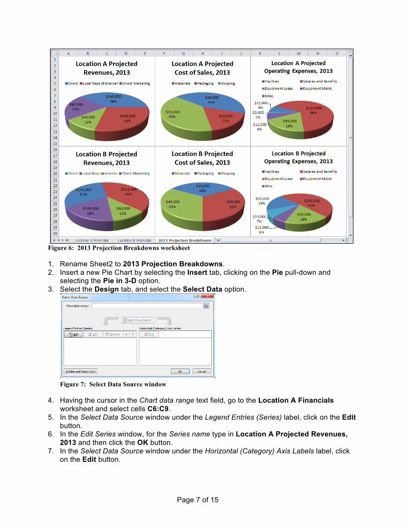
Figure 6: 2013 Projection Breakdowns worksheet

1. Rename Sheet2 to 2013 Projection Breakdowns. 2. Insert a new Pie Chart by selecting the Insert tab, clicking on the Pie pull-down and

selecting the Pie in 3-D option. 3. Select the Design tab, and select the Select Data option.

Figure 7: Select Data Source window

4. Having the cursor in the Chart data range text field, go to the Location A Financials worksheet and select cells C6:C9.

5. In the Select Data Source window under the Legend Entries (Series) label, click on the Edit button.

6. In the Edit Series window, for the Series name type in Location A Projected Revenues, 2013 and then click the OK button.

7. In the Select Data Source window under the Horizontal (Category) Axis Labels label, click on the Edit button.

of 15

8. In the Axis Labels window, for the Axis Label range go to Location A Financials worksheet and select cells A6:A9. Click the OK button.

9. In the Select Data Source window, click the OK button. 10. Under the Design tab in the Chart Layouts section, click the pull-down and select the Chart

Layout 2 option. 11. Position the chart so it approximately takes up the space from A1 through E15. 12. Click on the Pie Chart. Right-click, and select the Format Data Labels… option.

Figure 8: Format Data Label window

13. In the Format Data Label window, for the Label Contains checkboxes select the Value option. (Percentage and Show Leader Lines should already be checked.) For the Label Position radio buttons, select the Inside End (or Best Fit) option. For the Separator pull-down, select the (New Line) option. Click the Close button.

14. Under the Layout tab, click on the 3-D Rotation option. 15. In the Format Chart Area window, set the X value to 310, the Y value to 30, and the

Perspective value to 20. Click the Close button. 16. Under the Design tab, change the Chart Style to whatever you wish. 17. Select the Pie chart. Under the Format tab, click on the Shape Effects pull-down and select

the Bevel Circle option. This will soften the edge of the chart. 18. Change the size of the font of the Title so it fits nicely in the chart. Select the title, go to the

Home tab, and lower the size of the font, if necessary. 19. Repeat these same steps for the Location A Cost of Sales, Location A Operating

Expenses, Location B Revenues, Location B Cost of Sales, and Location B Operating Expenses. Try to get the values inside of the chat by changing the perspectives. Arrange the charts so that all three of Location A charts are on top and all three of Location B charts are on the bottom as shown in Figure 6.

of 15

Figure 9: Financial Trends worksheet

20. Rename Sheet3 to Financial Trends. If you need to add a new slide, click on the Insert Worksheet button at the bottom and then rename it.

21. Insert a new column chart by selecting the Insert tab, clicking on the Column pull-down and selecting the Clustered Column option.

22. Under the Design tab, click on the Select Data option. 23. In the Select Data Source window, under the Legend Entries (Series) label, click on the Add

button. 24. In the Edit Series window, for the Series name enter Location A Revenues. For the Series

values, delete the text that is there (by using the delete or backspace key). Go to the Location A Financials worksheet and highlight cells C10:E10. Click the OK button.

25. In the Select Data Source window, under the Horizontal (Category) Axis Labels label, click on the Edit button.

26. In the Axis Labels window for the Axis label range, click on the Location A Financials worksheet and select cells C4:E4. Click the OK button.

27. Back in the Select Data Source window, repeat the previous steps (23-26) for Location B Revenues, Location A Cost of Sales, Location B Cost of Sales, Location A Operating Expenses, and Location B Operating Expenses. You will need to use your brain and select the appropriate worksheet and cells. Once you are done, click the OK button.

28. Under the Design tab, click on the Chart Layouts pull-down and select Layout 7. 29. Under the Design tab, click on the Chart Styles pull-down and select Style 26. 30. Remove all axis layouts by clicking on the Layout tab and using the Axis Titles option to

remove both horizontal and vertical. 31. Add a chart tile by going to the Layout tab and selecting the Chart Title option. Enter the

title Revenue and Expense Projections.

of 15

Part 3 – Further Financial Analysis

Quite often, economic conditions govern which investment a company should make. The financial calculation of an investment’s net present value enables a company to consider these economic conditions and make an educated decision as to which investment to make. In this exercise, you will learn how to use Excel as a tool to make these kinds of informed decisions.

For this part of the project, you will be assessing the expansion of your business. Your company, whether it is a retailer or manufacturer, will be opening up a new location for business operations. You will choose between the two locations that you earlier created income statements. Each location will generate different revenues, which you previously estimated. This assignment will allow you to determine which location will be the most lucrative, based upon the prevailing economic conditions.

You will first use Excel’s built-in functions to “look up” values based upon certain criteria. Then, you will calculate the Net Present Value so as to compare investment in the two different locations with varying returns over the next three years under different economic inflationary conditions. Using an If-Then function, you will have Excel determine which location you should invest in. Then using a Payment function you will determine the required monthly payments when the cost of investing in each location is borrowed. Finally, you will chart the results of the Net Present Value calculations to “see” the complete potential of the two locations under the varying economic conditions and to determine at which inflationary rate both locations become equally attractive.

Figure 10: NPV worksheet

The NPV Sheet Layout Refer to Figure 10 for the following tasks.

1. Create a new worksheet by clicking on the Insert Worksheet icon at the bottom.

2. In the new worksheet, create the spreadsheet shown in Figure 10, including the cell formats

shown. Merge & center the text Net Present Value at Various Inflationary Rates in cells

of 15

F12:K12. The only numbers you will enter manually are the Square Footage and %NPV values.

3. For the %NPV rates (cells F13:K13), enter in 0, 0.01, 0.02, 0.03, 0.04, and 0.05, and then format them as a Percentage.

4. The text in cell A8 that display the tax rate needs to be wrapped. In the Home tab, click the Wrap Text button (which is above the Merge & Center button).

5. In cell A1, enter your name. 6. In cell H1, type in your USC email address. Then select this cell by right-clicking on it and

choose Hyperlink. Click on the e-mail address button on the left, and type in your USC email address.

7. Under Comparison of Two Locations, reference the Net Revenue/Loss amount from the Location A and Location B Financials worksheets for 2013, 2014, and 2015. For cell B15, you would reference cell C28 on the Location A Financials worksheet. You will not have a value for B14 and C14, which is the amount you would have paid for the locations today.

8. Rename the worksheet to NPV. The Purchase Costs Sheet Layout

Figure 11: Purchase Costs worksheet

Refer to Figure 11 for the following tasks.

9. Create a new worksheet. 10. In the new worksheet, enter the text and values as shown in Figure 11. 11. Format the numbers as currency with no cents. Format the interest rates as percentages. 12. Format the Purchase and Remodeling Costs Based Upon Square Footage data similar as it

appears above. Under the Home tab, use the Format as Table option. 13. Rename the worksheet to Purchase Costs. 14. Give the loan table a range name by highlighting cells B13:G14. Click on the Formulas tab,

select the Define Name option and enter LoanRates for the Name. Click the OK button. Alternatively, you may enter LoanRates in the Name Box.

15. In cells F3 and G3 reference the two locations’ square footage from the NPV worksheet. Do not simply type in their values. In the formula bar, enter an =, click the NPV sheet, click the appropriate cell, and hit the enter key.

of 15

16. In cells F4 and G4 use the VLOOKUP function to determine the purchase costs for the two different locations based upon the Purchase and Remodeling Cost table. For the VLOOKUP function for Location A, the first argument is F3, the second argument is $A$3:$C$9, and the third argument is 2 since we want the value from the second column.

17. In cells F5 and G5, use the VLOOKUP function to determine the remodeling costs for the two locations. For the third argument you want the value from the third column.

18. Use the AutoSum function in cells F6 and G6 to calculate the costs before taxes. Do not include the value for the Square Footage.

19. Save your workbook.

Calculate Total Cost: 20. Return to the NPV worksheet. 21. In cells B6 and C6, reference the purchase costs that were determined on the Purchase

Costs worksheet for Location A and Location B. 22. In cells B7 and C7, reference the remodeling costs that were determined on the Purchase

Costs worksheet for Location A and Location B. 23. In cells B8 and C8, calculate the 8.75% tax on the purchase cost of each location in cells B7

and C7 by using the appropriate formulas and cell references. For cell B8, enter =B6*8.75%. Display the results to the nearest dollar by utilizing the currency formatting.

24. In cells B9 and C9, use the AutoSum function to add up the total cost of the two locations after taxes. Be careful not to include the value for the square footage in your AutoSum calculation.

25. In cells B14 and C14, use cell references to include the cost of the two locations in the comparison table for Today. Since the values for the years are the net revenues/loss (if positive, then these are profits), the Today values for each location are the costs negated. For cell B14, the value is =-B9. These values should be negative which will be represented with a negative sign or parenthesis.

Calculate the loan amounts: 26. Return to the Purchase Costs worksheet. 27. In cells F7 and G7, use cell references to get the total cost from cells B9 and C9 from the

NPV worksheet. This is your loan amount. 28. To determine the annual interest rate for the two locations, an HLOOKUP will be necessary.

In cell F9, use the HLOOKUP function to get the interest rate. The first argument will be the total cost, since the interest rate is dependent on the principle. The second argument is the table LoanRates. The third argument is the row index number, which is 2 since we are trying to retrieve the values from the second row of the LoanRates table.

29. Change the format of cells F9 and G9 to Percentage. 30. In cells F10 and G10, calculate the monthly payments for the loan amount using the PMT

function. a. The first argument for the PMT function is the interest rate for the period of the payment.

Since our interest rate is annual, and our payments are monthly, we have to divide by 12. So the value should reference cells F9 and G9, divided by 12.

b. The second argument for the PMT function is the number of payments. Since there are 12 months in a year and we have a 3 year loan, the value is 36.

of 15

c. The third argument for the PMT function is the present value. Since this is a loan, use the loan amount.

Calculate the NPV values: 31. Return to the NPV sheet. 32. Use the NPV function in cells F14:K15 to calculate the Net Present Values for the two

locations under different inflationary rates. a. The first argument for the NPV function is the rate of discount over the length of one

period. This is the inflationary rate. For cell F14, this argument is F13. b. The second argument is a range for the income. For cell F14 which is for Location A,

this argument is $B$15:$B$17. For cells that need to reference Location B, use $C$15:$C$17.

c. For the cells F14:K15, the value of Today needs to be added to the NPV result. For cell F14, the value is NPV(…)+$B$14.

33. In cells D19 and D20, use an appropriate IF function to have Excel determine the correct answers to the two questions in rows 19 and 20 based upon the results of your NPV calculations. a. The first argument for the IF function is the logical test. Compare the values in the Net

Present Values table. For cell D19 which asks at 1% inflation, this argument is G14>G15.

b. The second argument for the IF function is the value if the logical test is true. For cell D19, we want to print the text Location A since location A would be more appealing. Thus this argument is E14.

c. The third argument for the IF function is the value if the logical test is false. For cell D19, we want to print the text Location B since location B would be more appealing. Thus this argument is E15.

34. In cells D21 and D22, reference the monthly payment values calculated on the Purchase Costs worksheet. Do not simply type in the calculated values from the sheet.

Creating the NPV chart:

Figure 12: Sample NPV Chart

On the NPV worksheet, create a line chart displaying the NPV values. Your chart data will differ from the above chart, and hence will not look identical. Adjust your commentary accordingly. 35. Select the range of cells you want to use for the chart (E13:K15).

of 15

36. Select the Insert tab, click on the Line option (in the Charts area) and select the 2-D Line chart.

37. Under Chart Tools, select the Layout tab. Use the Chart Title option to add the following title above the chart: Net Present Value Calculation.

38. Use the Axis Titles option to add the following title to the Horizontal Axis below the values: Inflationary Rates.

39. Remove the chart’s background pattern and border by selecting Plot Area None. 40. Remove the gridlines by selecting Gridlines Primary Horizontal Gridlines None and

Gridlines Primary Vertical Gridlines None. 41. Change the two Location NPV data lines to a heavier weighted line. Select each line and

click on the Format Selection option. Click on the Line Style option, and change the Width to 4 pt.

42. Change the Y-axis. Select the Vertical (Value) Axis section in the chart and click on the Format Selection option. In the Axis Options section of the Format Axis window, for the Minimum option select the Fixed radio button and change the value in the text field to be major dollar amount below the lines. Change the Maximum option to be a value above the lines. Make sure the Major unit amount is 50000. Select the Number option, and change the Category to Currency and the Decimal places text field to 0. Click the Close button.

43. Make sure the tick marks cross the X and Y-axes, and the X-axis labels should align with the tick marks. a. Click on the Horizontal (Category) Axis section in the chart, and select the Format

Selection option. In the Format Axis window, make sure the Axis Options is selected. For the Major tick mark type, change the pull-down to Cross. For the Position Axis, select the On tick marks radio button. Click the Close button.

b. Click on the Vertical (Value) Axis section in the chart, and select the Format Selection option. For the Major tick mark type, change the pull-down to Cross. Click the Close button.

44. Add a Text Box to the chart. Under the Layout tab in the Insert section, click the Text Box icon. a. If the two lines cross, then the two locations are equally attractive at the corresponding

inflation rate. In the text box, enter a message stating the inflation rate such as “The locations are equally attractive at 10%.”

b. If the two lines do not intersect, then one location is always preferable. In the text box, enter a message stating the preferable location such as “Location A is preferable.”

Final checks: 45. Verify all dollar amounts are to the nearest dollar (no decimals) on all sheets. Every dollar

amount should be formatted using the standard accounting format. 46. To test the project once you have finished, change the Square Footage on the NPV

worksheet. For example, change Location A to 6000 and Location B to 8000. All the cell values that you calculated, including the Chart, should change.

47. Change the square footage back to 5575 for Location A and 3750 for Location B. 48. Save your workbook.

of 15

Submitting the project

1. There should be a total of 6 worksheets in your Excel workbook. Arrange them in the following order: Location A Financials, Location B Financials, 2013 Projection Breakdowns, Financial Trends, NPV, Purchase Costs.

2. Save the Excel file as lastname_firstname_excel.xlsx, where lastname and firstname are replaced with your lastname and firstname.

3. Submit your Excel file on Blackboard (http://blackboard.usc.edu) under Assignments. a. Click on the Lab4 assignment. b. Next to Attach File, click on the Browse My Computer button. c. Find your lastname_firstname_excel.xlsx file and click the Choose button. d. Click on the Submit button in the bottom right corner.

Project 4 Financials (Excel) - Personal World Wide Web...

Documents

Transcript of Project 4 Financials (Excel) - Personal World Wide Web...