Progressive Indexes

Progressive IndexesTimbó Holanda, P.T.

CitationTimbó Holanda, P. T. (2021, September 21). Progressive Indexes. SIKS Dissertation Series.Retrieved from https://hdl.handle.net/1887/3212937 Version: Publisher's Version

License: Licence agreement concerning inclusion of doctoral thesis in theInstitutional Repository of the University of Leiden

Downloaded from: https://hdl.handle.net/1887/3212937 Note: To cite this publication please use the final published version (if applicable).

https://hdl.handle.net/1887/license:5

https://hdl.handle.net/1887/license:5

https://hdl.handle.net/1887/3212937

CHAPTER 3

Progressive Indexing

1 Introduction

Data scientists perform exploratory data analysis to discover unexpected patterns in

large collections of data. This process is done with a hypothesis-driven trial-and-error

approach [52]. They query data segments that could potentially provide insights, test

their hypothesis, and either zoom in on the same segment or move to a different one

depending on the insights gained.

Fast responses to queries are crucial to allow for interactive data exploration. The

study by Liu et al. [41] shows that any delay larger than 500ms (the “interactivity

threshold”) significantly reduces the rate at which users make observations and

generate hypotheses. When dealing with small data sets, providing answers within

this interactivity threshold is possible without utilizing indexes. However, exploratory

data analysis is often performed on larger data sets as well. In these scenarios, indexes

are required to speed up query response times.

Index creation is one of the major difficult decisions in database schema design [15].

Based on the expected workload, the database administrator (DBA) needs to decide

whether creating a specific index is worth the overhead in creating and maintaining

it. Creating indexes up-front is especially challenging in exploratory and interactive

data analysis, where queries are not known in advance, workload patterns change

frequently, and interactive responses are required. In these scenarios, data scientists

load their data and immediately want to start querying it without waiting for index

27

1. Introduction

construction. In addition, it is also not certain whether or not creating an index

is worth the investment at all. We cannot be sure that the column will be queried

frequently enough for the large initial investment of creating a full index to pay off.

In spite of these challenges, indexing remains crucial for improving database

performance. When no indexes are present, even simple point and range selections

require expensive full table scans. When these operations are performed on large

data sets, indexes are essential to ensure interactive query response times. Two main

strategies aim to release the DBA of having to choose which indexes to create manually.

(1) Automated index selection techniques [1, 14, 58, 23, 13, 11, 44, 53] accomplish

this by attempting to find the optimal set of indexes given a query workload, taking

into account the benefits of having an index versus the added costs of creating the

entire index and maintaining it during modifications to the database. However, these

techniques require a priori knowledge of the expected workloads and do not work well

when the workload is not known or changes frequently. Hence they are not suitable

for interactive data exploration.

(2) Adaptive Indexing techniques such as Database Cracking [36, 21, 50, 49, 26,

35, 37, 47, 46, 25, 34, 29] are a more promising solution. They focus on automatically

and incrementally building an index as a side effect of querying the data. An index

for a column is only initiated when it is first queried. As the column is queried more,

the index is refined until it eventually approaches a full index’s performance. In this

way, the cost of creating an index is smeared out over the cost of querying the data

many times, though not necessarily equally, and there is a smaller initial overhead

for starting the index creation. However, since the index is refined only in the areas

targeted by the workload, convergence to a full index is not guaranteed, and partitions

can have different sizes. The query’s performance degrades when a less refined part of

the index is queried, resulting in performance spikes whenever the workload changes.

In this chapter, we introduce a new incremental indexing technique called Progres-

sive Indexing. It differs from other indexing solutions in that the indexing budget (i.e.,

the amount of time spent on index creation and refinement) can be controlled. We

provide two indexing budget flavors: a fixed indexing budget, where the user defines a

fixed amount of time to spend on indexing per query, and an adaptive indexing budget,

where the indexing budget is adapted so that the total time spent on query execution

remains constant. We refer to the fixed indexing budget as Progressive Indexing

and the adaptive indexing budget as Greedy Progressive Indexing. As a result, both

Progressive Indexing and Greedy Progressive Indexing complements existing automatic

indexing techniques by offering predictable performance and deterministic convergence

28

Chapter 3. Progressive Indexing

independent of the workload.

1.1 Contributions

The main contributions of this chapter are:

• We introduce several novels Progressive Indexing techniques and investigate

their performance, convergence, and robustness in the face of various realistic

synthetic workload patterns and real-life workloads.

• We provide a cost model for each of the Progressive Indexing techniques. The

cost models are used to adapt the indexing budget automatically.

• We experimentally verify that the Progressive Indexing techniques we propose

provide robust and predictable performance and convergence regardless of the

workload or data distribution.

• We provide a decision tree to assist in choosing an indexing technique for a given

scenario.

• We provide Open-Source implementations of each of the techniques we describe

and their benchmarks.1

1.2 Outline

This chapter is organized as follows. Section 2 depicts related research performed on

automatic/adaptive index creation. In Section 3, we describe our novel Progressive

Indexing techniques and discuss their benefits and drawbacks. Section 4 describes

the cost-models used to adapt our indexing budget automatically. In Section 5, we

perform an experimental evaluation of each of the novel methods we introduce, and

we compare them against Adaptive Indexing techniques. Finally, in Section 6 we draw

our conclusions and present a decision tree to assist in choosing which Progressive

Indexing technique to use.

2 Related Work

In this section, we discuss the state-of-the-art of Adaptive Indexing in terms of

performance and robustness. Section 2.1 we discuss possible cracking kernels to get

1Our implementations and benchmarks are available at https://github.com/pdet/

ProgressiveIndexing

29

https://github.com/pdet/ProgressiveIndexing

https://github.com/pdet/ProgressiveIndexing

2. Related Work

the partitioning as fast as possible. In Section 2.2 we discuss three different Adaptive

Indexing algorithms that attempt to improve cracking’s robustness problem.

2.1 Cracking Kernels

A cracking kernel [47, 25] is the central part of how the partitioning of a piece is

done. This section focuses on two partitioning kernels. First, we present the branching

kernel, which uses if-else clauses to decide when to swap elements. Second, we describe

the predicated kernel that uses predication to avoid branch mispredictions.

Branching Kernel

The branching kernel is the one used in the Standard Cracking implementation and

has a clear inspiration from quicksort’s partitioning [27]. Listing 1 depicts the kernel

for the integer data type. It receives as input the array, the pivot, and the boundaries

of the partition posL and posR. The algorithm, inspects all vector elements, and

increase posL in case the element data[posL] is less than the pivot and increases posR

in case the element data[posR] is greater than or equal to the pivot. In other words,

it simply moves the cursors if the elements are already in the correct position in

reference to the pivot. If it finds both data[posL] and data[posR] that are not in the

correct position, it swaps them and move the cursors. The main problem with this

kernel is that swapping the data in the if-else clauses causes an increase in branch

mispredictions and an overall decrease in performance, as demonstrated in Boncz et

al. [10].

Listing 1 Branching Kernel

1 void branching_kernel(int& data, int pivot, size_t posL, size_t posR){

2 while (posL < posR){

3 if (data[posL] < pivot){

4 posL++;

5 }

6 else if (data[posR]>= pivot{

7 posR--;

8 }

9 else{

10 swap(data[posL++],data[posR--])

11 }

12 }

13 }

30


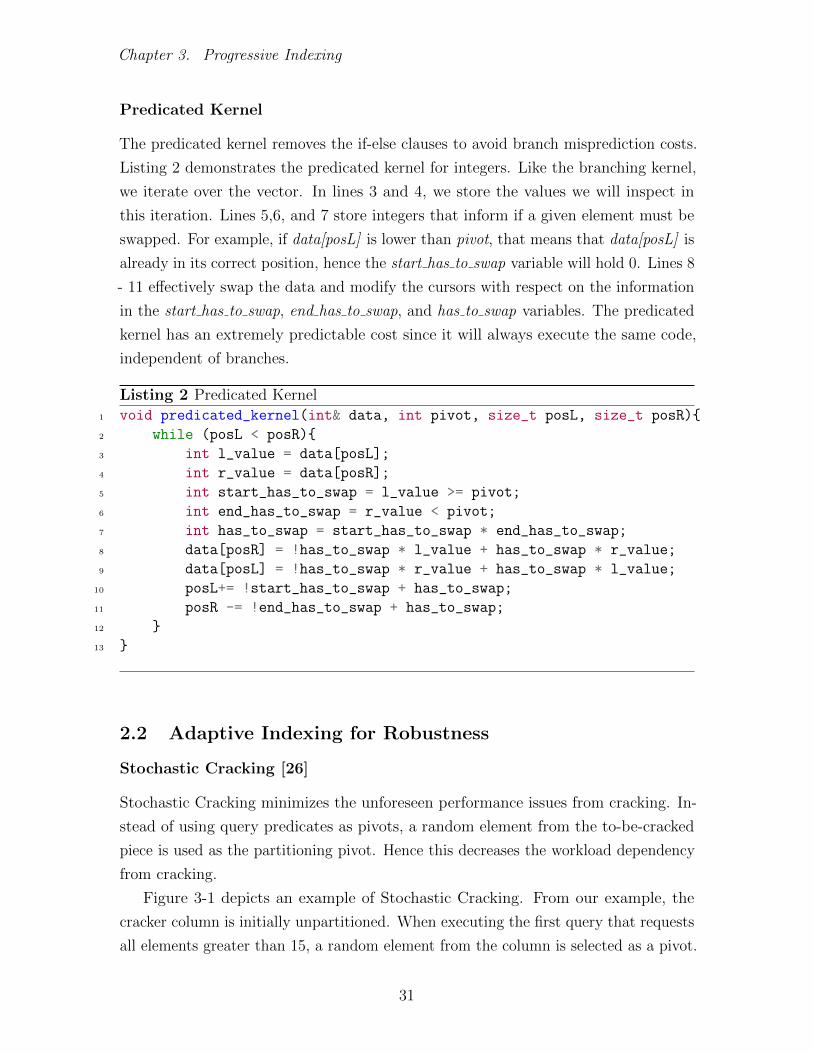
Predicated Kernel

The predicated kernel removes the if-else clauses to avoid branch misprediction costs.

Listing 2 demonstrates the predicated kernel for integers. Like the branching kernel,

we iterate over the vector. In lines 3 and 4, we store the values we will inspect in

this iteration. Lines 5,6, and 7 store integers that inform if a given element must be

swapped. For example, if data[posL] is lower than pivot, that means that data[posL] is

already in its correct position, hence the start has to swap variable will hold 0. Lines 8

- 11 effectively swap the data and modify the cursors with respect on the information

in the start has to swap, end has to swap, and has to swap variables. The predicated

kernel has an extremely predictable cost since it will always execute the same code,

independent of branches.

Listing 2 Predicated Kernel

1 void predicated_kernel(int& data, int pivot, size_t posL, size_t posR){

2 while (posL < posR){

3 int l_value = data[posL];

4 int r_value = data[posR];

5 int start_has_to_swap = l_value >= pivot;

6 int end_has_to_swap = r_value < pivot;

7 int has_to_swap = start_has_to_swap * end_has_to_swap;

8 data[posR] = !has_to_swap * l_value + has_to_swap * r_value;

9 data[posL] = !has_to_swap * r_value + has_to_swap * l_value;

10 posL+= !start_has_to_swap + has_to_swap;

11 posR -= !end_has_to_swap + has_to_swap;

12 }

13 }

2.2 Adaptive Indexing for Robustness

Stochastic Cracking [26]

Stochastic Cracking minimizes the unforeseen performance issues from cracking. In-

stead of using query predicates as pivots, a random element from the to-be-cracked

piece is used as the partitioning pivot. Hence this decreases the workload dependency

from cracking.

Figure 3-1 depicts an example of Stochastic Cracking. From our example, the

cracker column is initially unpartitioned. When executing the first query that requests

all elements greater than 15, a random element from the column is selected as a pivot.

31

2. Related Work

Figure 3-1: Standard Cracking executing two queries.

In our example, the element 7, the column is then partitioned around 7, and both

pieces must be scanned to answer the query. When query 2 is executed requesting

all elements between 5 and 15, Piece 1 is pivoted with an element within the piece,

in this case, 4, and the same happens with Piece 2, with pivot 16 being selected to

partition it. After finishing the partition, only piece 2 (i.e., all elements over 4) and

piece 3 (i.e., all elements higher than 7 and lower or equal to 16) must be scanned.

Not using the filter predicates as query pivots can result in the execution engine

reading more data than necessary even after the partitioning for that query. However,

sudden changes in the workload pattern will not have the same impact as in Standard

Cracking.

Progressive Stochastic Cracking [26]

Progressive Stochastic Cracking progressively performs Stochastic Cracking. It takes

two input parameters, the size of the L2 cache and the number of swaps allowed in

one iteration (i.e., a percentage of the total column size). When performing Stochastic

Cracking, Progressive Stochastic Cracking will only perform at most the maximum

allowed number of swaps on pieces larger than the L2 cache. If the piece fits into the

32


L2 cache, it will always perform a complete crack of the piece.

Figure 3-2: Progressive Stochastic Cracking with maximum swaps = 2 and L2 CacheSize = 8kb.

Figure 3-2 depicts an example of Progressive Stochastic Cracking, where the L2

Cache Size fits two integers and the at most two swaps can be performed per query.

Like Stochastic Cracking, the pivots are also selected randomly from within the piece

that will be partitioned. In our first query, the pivot chosen is 7. The difference is

that when executing this query, we stop pivoting after swapping two elements. When

executing Query 2, we finish the partition with pivot 7 before picking new pivots.

Coarse-Granular Index [50]

The Coarse-Granular Index improves Stochastic Cracking’s robustness by creating k

partitions when the first query is executed using equal-width binning. It also allows

for creating any number of partitions instead of limiting the number of partitions to

two, letting the DBA decide on k , choosing between the trade-off of the higher cost of

the first query versus building a more robust index.

Figure 3-3 depicts an example of the Coarse-Granular Index set to create four

partitions. When executing the first query, the algorithm will perform 3 cracking

33

2. Related Work

Figure 3-3: Coarse Granular-Index creating k = 4 partitions in the first query.

iterations from the equi-width binning (i.e., since our data goes from 1 to 20, that

means the pivots will be 5,10, and 15). After it, a standard Stochastic Cracking

iteration happens. At that point, it is only necessary to check Piece 4 since it holds

all elements over 15. A random pivot from within the piece is selected, in this case,

16, and the query answer is produced.

Adaptive Adaptive Indexing [49]

Adaptive Adaptive Indexing is a general-purpose algorithm for Adaptive Indexing. It

has multiple parameters tuned to mimic the data access of different Adaptive Indexing

techniques (e.g., Database Cracking, Sideways Cracking, Hybrid Cracking). It also

uses radix partitioning and exploits software-managed buffers using nontemporal

streaming stores to achieve better performance [51].

34


��

⇢

��

��

⇢

After 3 Queries After 4 Queries After 10 Queries

�

��

�

⇢

�

Figure 3-4: Creation phase of Progressive Indexing.

3 Progressive Indexing

In this section, we introduce Progressive Indexing. The core features of Progressive

Indexing are that (1) the indexing overhead per query is controllable, both in terms

of time and memory requirements, (2) it offers robust performance and deterministic

convergence regardless of the underlying data distribution, workload patterns, or query

selectivity, and (3) the indexing budget can be automatically tuned so more expensive

queries spend less extra time on indexing while cheaper queries spend more. To allow

for robust query execution times regardless of the data, we avoid branches in the code

and use predication when possible [48, 10].

As a result of the small initial cost, Progressive Indexing occurs without significantly

impacting worst-case query performance. Even if the column is only queried once,

only a small penalty is incurred. On the other hand, if the column is queried hundreds

of times, the index will reliably converge towards a full index, and queries will be

answered at the same speed as with an a-priori built full index.

All Progressive Indexing algorithms progress through three canonical phases to

eventually converge to a full B+-tree index: the creation phase, the refinement phase,

and the consolidation phase. Each phase’s work can be divided between multiple

queries, keeping the extra indexing effort per query strictly limited.

35

3. Progressive Indexing

Creation Phase. The creation phase progressively builds an initial “crude”

version of the index by adding another δ fraction of the original column to the index

with each query. Query execution during the creation phase is performed in three

steps(visualized in Figure 3-4):

1. Perform an index lookup on the ρ fraction of the data that has already been

indexed;

2. Scan the not-yet-indexed 1− ρ fraction of the original column;

and while doing so,

3. Expand the index by another δ fraction of the total column.

As the index grows and the fraction ρ of the indexed data increases, an ever-

smaller fraction of the base column has to be scanned, progressively improving query

performance. Once all the base column data has been added to the index, the creation

phase is followed by the refinement phase.

Refinement Phase. With the base column no longer required to answer queries,

we only perform lookups into the index to answer queries. While doing these lookups,

we further refine the index, progressively converging towards a fully ordered index.

In the refinement phase, we focus on refining parts of the index required for query

processing. After these parts have been refined, the refinement process starts processing

the neighboring parts. Once the index is fully ordered, the refinement phase is followed

by the consolidation phase.

Consolidation Phase. With the index fully ordered, we progressively construct

a B+-tree from it since a B+-Tree provides better data locality and thus is more

efficient than binary search when executing very selective queries. Once the B+-tree

is completed, we use it exclusively to answer all subsequent queries. The consolidation

phase is the same for all progressive algorithms. All algorithms end their refinement

phase with a sorted array. The B+-tree is then constructed on top of that sorted array

in a bottom-up fashion. Figure 3-5 depicts an example of the construction phase for

Progressive Quicksort in the right-most part of the figure labeled Consolidation. In

this example, the B+-Tree stored 4 elements per node. Hence we start constructing

the last level of the inner nodes pointing to one element every four elements. In this

case, the B+-Tree nicely ends with one inner node that is also the root. However,

if there were more elements, we would fully construct this level, link all nodes, and

proceed to the upper level and repeat this strategy.

36


In the following section, we discuss the details of four different Progressive Indexing

implementations. Section 3.1 describes Progressive Quicksort as a progressive version

of quicksort, aiming to achieve good performance independent of query patterns and

data distributions. In Section 3.2 we present Progressive Radixsort - Most Significant

Digit as the radixsort algorithm this index is based on, we expect good performance

over uniform distributions. In Section 3.3 we present Progressive Bucketsort, inspired

by bucketsort equi-height, which is expected to present excellent performance with

highly skewed data distributions. Finally, in Section 3.4 we present Progressive

Radixsort - Least Significant Digit, where we aim to optimize for workloads that

contain only point queries.

3.1 Progressive Quicksort

Figure 3-5 depicts snapshots of the creation phase, the refinement phase, and the

consolidation phase of Progressive Quicksort. We discuss the creation and refinement

phases in detail in the following paragraphs.

1619

7

14

1313

1

14

8

911

1

63

63161321819712114914

Original Column

A ≤ 10

10 < A

6

16

2

Uni

nitia

lized

Initialize

32

8914111213

Initialize 2

A ≤ 10

10 < A

A ≤ 7

7 < A

A ≤ 15

15 < A

Refinement

Pivo

t=10

Pivo

t=15

Pivo

t=7

1413

46

123

78

12

1619

ConsolidationSo

rted

161114

B+ T

ree

A ≤ 10

10 < A Pivo

t=10

7

632

49

111219

16

Figure 3-5: Progressive Quicksort.

37


Creation Phase

In the first iteration, we allocate an uninitialized column of the same size as the

original column and select a pivot. The pivot is selected by taking the average value

of the smallest and largest value of the column. In Figure 3-5, pivot 10 is the average

of 1 and 19. If sufficient statistics are available, the median value of the column could

be used instead. Unlike Adaptive Indexing, the pivot selection is not impacted by the

query predicates. We then scan the original column and copy the first N ∗ δ elements

to either the top or bottom of the index, depending on their relation to the pivot. In

this step, we also search for any elements that fulfill the query predicate and afterward

scan the not-yet-indexed 1− ρ fraction of the column to compute the complete answer

to the query. In subsequent iterations, we scan either the top, bottom, or both parts

of the index based on how the query predicate relates to the chosen pivot.

Refinement Phase

We refine the index by recursively continuing the quicksort in-place in the separate

sections. The refinement consists of swapping elements in-place inside the index around

the pivots of the different segments. When the pivoting of a segment is completed, we

recursively continue the quicksort in the child segments. We maintain a binary tree

of the pivot points. In this tree’s nodes, we keep track of the pivot points and how

far along the pivoting process we are. To do an index lookup, we use this binary tree

to find the array sections that could match the query predicate and only scan those,

effectively reducing the amount of data to be accessed even when the full pivoting has

not been completed yet.

When we reach a node that is smaller than the L1 cache, we sort the entire node

instead of recursing any further. After sorting a node entirely, we mark it as sorted.

When two children of a node are sorted, the entire node itself is sorted, and we can

prune the child nodes. As the algorithm progresses, leaf nodes will keep on being

sorted and pruned until only a single fully sorted array remains.

3.2 Progressive Radixsort (MSD)

Figure 3-6 depicts snapshots of the creation phase, the refinement phase, of Progressive

Radixsort (MSD). We discuss both phases in detail in the following paragraphs.

38


11

4

1

13

8

14

11

3

16

16

13

3

19

8

1414

1

63141321819712114169

6

2

Initialize Refinement

00…

13

11

17

632

4

12

9

01…

10…

11…

Uni

nitia

lized

19

00.

01.

10.

11.

1

2467

00.

01.

10.

11.

9

12

00…

01…

10…

Refinement

13

8

14

11

3

00.

01.

10.

11.

1

2467

00.

01.

10.

11.

9

12

9

16

13

6

23

78

12

14

19

Original Column

Figure 3-6: Progressive Radixsort (MSD).

Creation Phase

In the creation phase of Progressive Radixsort, we perform the radixsort partitioning

into buckets located in separate memory regions. We start by allocating b empty

buckets. Then, while scanning the original column, we place N ∗ δ elements into the

buckets based on their most significant log2 b bits. We then scan the remaining 1− ρfraction of the base column. In subsequent iterations, we scan the [0, b] buckets that

could potentially contain elements matching the query predicate to answer the query

in addition to scanning the remainder of the base column.

Bucket Count. Radix clustering performs a random memory access pattern that

randomly writes in b output buckets. To avoid excessive cache- and TLB-misses,

assuming that each bucket is at least of the size of a memory page, the number b of

buckets, and thus the number of randomly accessed memory pages, should not exceed

the number of cache lines and TLB entries, whichever is smaller [9]. Since our machine

has 512 L1 cache lines and 64 TLB entries, we use b = 64 buckets.

Bucket Layout. To avoid allocating large regions of sequential data for every

bucket, the buckets are implemented as a linked list of blocks of memory that each

39


hold up to sb elements. When a block is filled, another block is added to the list,

and elements will be written to that block. This adds some overhead over sequential

reads/writes as for every sb elements there will be a memory allocation and random

access, and for every element that is added, the bounds of the current block have to

be checked.

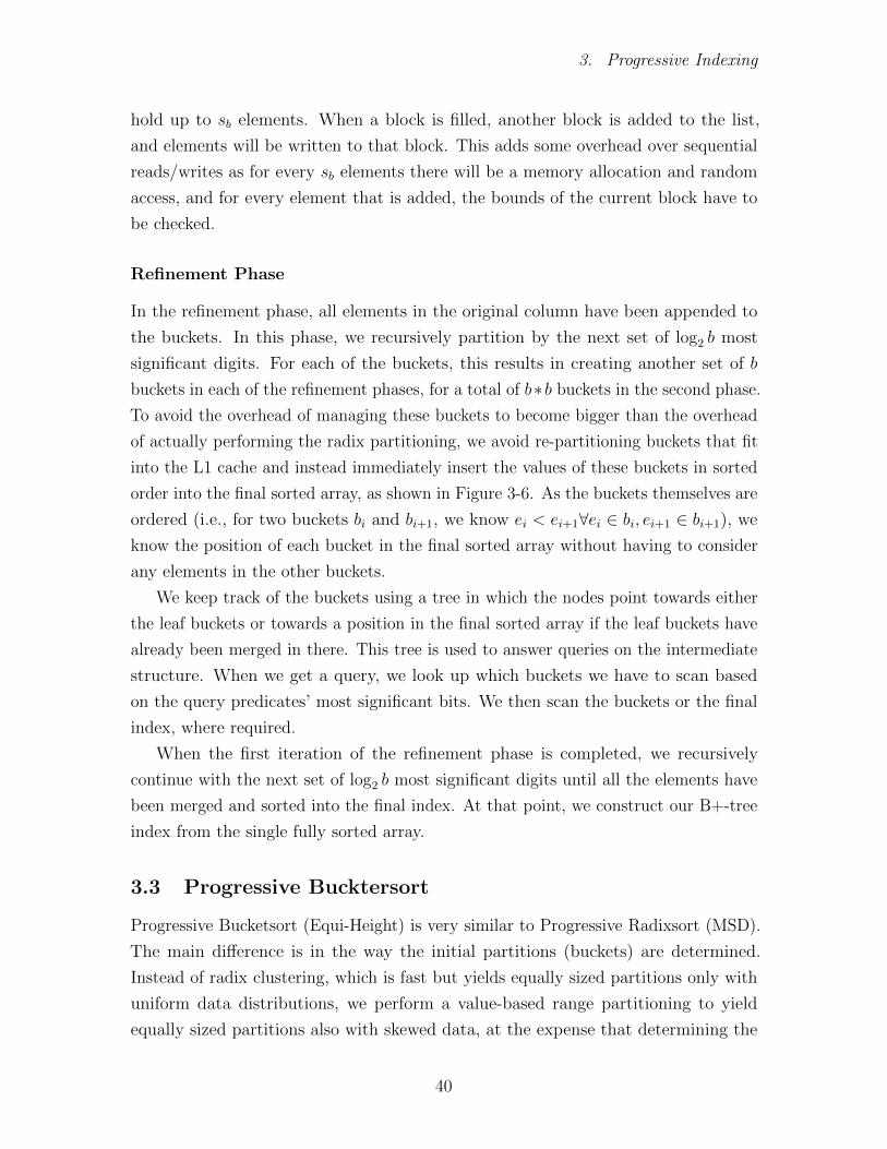
Refinement Phase

In the refinement phase, all elements in the original column have been appended to

the buckets. In this phase, we recursively partition by the next set of log2 b most

significant digits. For each of the buckets, this results in creating another set of b

buckets in each of the refinement phases, for a total of b∗b buckets in the second phase.

To avoid the overhead of managing these buckets to become bigger than the overhead

of actually performing the radix partitioning, we avoid re-partitioning buckets that fit

into the L1 cache and instead immediately insert the values of these buckets in sorted

order into the final sorted array, as shown in Figure 3-6. As the buckets themselves are

ordered (i.e., for two buckets bi and bi+1, we know ei < ei+1∀ei ∈ bi, ei+1 ∈ bi+1), we

know the position of each bucket in the final sorted array without having to consider

any elements in the other buckets.

We keep track of the buckets using a tree in which the nodes point towards either

the leaf buckets or towards a position in the final sorted array if the leaf buckets have

already been merged in there. This tree is used to answer queries on the intermediate

structure. When we get a query, we look up which buckets we have to scan based

on the query predicates’ most significant bits. We then scan the buckets or the final

index, where required.

When the first iteration of the refinement phase is completed, we recursively

continue with the next set of log2 b most significant digits until all the elements have

been merged and sorted into the final index. At that point, we construct our B+-tree

index from the single fully sorted array.

3.3 Progressive Bucktersort

Progressive Bucketsort (Equi-Height) is very similar to Progressive Radixsort (MSD).

The main difference is in the way the initial partitions (buckets) are determined.

Instead of radix clustering, which is fast but yields equally sized partitions only with

uniform data distributions, we perform a value-based range partitioning to yield

equally sized partitions also with skewed data, at the expense that determining the

40


131416

87

16

346

11

4

19

13

76

9

46

12

63141321819712114169

Original Column

3

1

Initialize Refinement

23

12

19

Refinement

A<5

9

11

321

8

12

14A<

5 A < 3

3<=A

5<=A

<10

10<=

A<14

14<=

A<20

21

A < 5

5<=A

Uni

nitia

lized

Sorte

d

A < 10

10<=A

1314

5<=A

<10

10<=

A<14

14<=

A<20 So

rted

A < 8

8<=A

A < 5

5<=A

Figure 3-7: Progressive Bucket Sort

bucket that a value belongs to is more expensive. Figure 3-7 depicts a snapshot of

the creation phase and two snapshots of the refinement phase. In the following, we

discuss these two phases in detail.

Bucket Count. To optimize for writing and reading from the buckets, our

implementation of Progressive Bucketsort uses 64 buckets, as discussed in Section 3.2.

Creation Phase

Progressive Bucketsort operates in a very similar way to Progressive Radixsort (MSD).

Instead of choosing the bucket an element belongs to based only on the most significant

bits, the bucket is chosen based on a set of bounds that more-or-less evenly divide

the set elements into the separate buckets. These bounds can be obtained either in

the scan to answer the first query or from existing statistics in the database (e.g., a

histogram).

41


Refinement Phase

In the refinement phase, all elements in the original column have been appended to the

buckets. We then merge the buckets into a single sorted array. Unlike with Progressive

Radixsort (MSD), we do not recursively keep on using Progressive Bucketsort. This

is because the overhead of finding and maintaining the equi-height bounds for each

sub-bucket is too large. Instead, we sort the individual buckets into the final sorted list

using Progressive Quicksort. Using a progressive algorithm to sort individual buckets

protects us from performance spikes caused by sorting large buckets.

The buckets are merged into the final sorted index in order. As such, we always

have a single iteration of Progressive Quicksort active at a time in which we are

performing swaps. After all the buckets have been merged and sorted into the final

index, we have a single fully sorted array from which we can construct our B+-tree

index.

3.4 Progressive Radixsort (LSD)

9

193

137

136

14

1

6

2

63141321819712114169

Original Column Initialize Refinement Refinement

…00

8

13

23

…00

…01

…10

…11

14

…01

…10

…113

1

19

12

11

416

9

.00.

..0

1..

.10.

..1

1..

8

12

4

16

6

0….

1….

4

8

16

6

1213

.00.

..0

1..

.10.

..1

1..

1

14

2

7

11

1619

12346

Figure 3-8: Progressive Radixsort (LSD).

42


Progressive Radixsort Least Significant Digits (LSD) performs a progressive radix

clustering on the least significant bits during the creation and refinement phase.

Figure 3-8 depicts a snapshot of the creation phase and two snapshots of the refinement

phase. In the following, we discuss these two phases in detail.

Bucket Count. To optimize for writing and reading from the buckets, our

implementation of Progressive Radixsort (LSD) uses 64 buckets, as discussed in

Section 3.2.

Creation Phase

This algorithm’s creation phase is similar to the creation phase of Progressive Radixsort

(MSD), except that we partition elements based on the least-significant bits instead of

the most-significant bits. We can use the buckets created to speed up point queries

because we only need to scan the bucket in which the query value falls. However,

unlike the buckets created for the Progressive Radixsort (MSD) and Progressive

Bucketsort, these intermediate buckets cannot be used to speed up range queries in

many situations. Because the elements are inserted based on their least-significant bits,

the buckets do not form a value-based range-partitioning of the data. Consequently,

we will have to scan many buckets, depending on the domain covered by the range

query.

Refinement Phase

In the refinement phase, we move elements from the current set of buckets to a new set

of buckets based on the next set of significant bits. We repeat this process until the

column is sorted. How many iterations this takes depends on the bucket count and the

column’s value domain, which we obtain from the [min,max] values. We can compute

the amount of required iterations with the formula dlog2(max−min)/log2(b)e. For

example, for a column with values in the range of [0, 216) and 64 buckets, the amount

of iterations required before convergence is dlog2(216)/log2(64)e = 3.

4 Greedy Progressive Indexing

The value of δ determines how much time is spent constructing the index and hence

determines the indexing budget. Greedy Progressive Indexing allows the user to select

between setting either a fixed indexing budget or an adaptive indexing budget. For

the fixed indexing budget, the user provides the desired indexing budget tbudget to

43

4. Greedy Progressive Indexing

Table 3.1: Parameters for Greedy Progressive Quicksort Cost Model.System ω cost of sequential page read (s)

κ cost of sequential page write (s)φ cost of random page access (s)γ elements per page

Data set N number of elements in the data set& Query α % of data scanned in partial indexIndex δ % of data to-be-indexed

ρ % of data already indexedProgressive Quicksort h height of the binary search treeProgressive b number of bucketsRadixsort sb max elements per bucket block

τ cost of memory allocation (s)B+-Tree β tree fanout

spend on indexing for the first query. We then select the value of δ based on this

budget and use that δ for the remainder of the workload. The adaptive indexing

budget allows the user to specify the desired indexing budget for the first query tbudget.

The first query will then execute in time tadaptive = tscan + tbudget. After the first query,

the value of δ will be adapted such that the query cost will stay equivalent to tadaptive

until the index is converged.

Cost Model. We use a cost model to determine how much time we can spend on

indexing when working with the adaptive indexing budget. The cost model takes into

account the query predicates, the selectivity of the query and the state of the index in

a way that is not sensitive to different data distributions or querying patterns and

does not rely on having any statistics about the data available.

4.1 Greedy Progressive Quicksort

The parameters of the Greedy Progressive Quicksort cost model are summarized in

Table 3.1.

Creation Phase

The total time taken in the creation phase is the sum of (1) the scan time of the

base table, (2) the index lookup time, and (3) the additional indexing time. The scan

time is given by multiplying the number of pages we need to scan (Nγ

) by the amount

of time it takes for a sequential page access (ω), resulting in tscan = ω ∗ Nγ

. The

pivoting time (i.e., index construction time) consists of scanning the base table pages

and writing the pivoted elements to the result array. The pivoting time is therefore

44


obtained by multiplying the time it takes to scan and write a page sequentially (κ+ω)

by the number of pages we need to write, resulting in tpivot = (κ+ ω) ∗ Nγ

.

The total time taken for the initial indexing process is given by multiplying the

scan time by the fraction of the base table we need to scan. Initially, we need to scan

the entire base table, but as the fraction of indexed data (ρ) increases, we need to scan

less. Instead, we scan the index to answer the query. The amount of data we need

to scan in the index depends on how the query predicates relate to the pivot. The

fraction of data that we need to scan is given by α and can be computed for a given

set of query predicates. The total fraction of the data that we scan is 1− ρ+ α− δ.The fraction of the data that we index in each step is δ. Hence the total time taken is

given by ttotal = (1− ρ+ α− δ) ∗ tscan + δ ∗ tpivot.Indexing Budget. In this phase, we set delta such that δ =

tbudgettpivot

. For the fixed

indexing budget, we select this δ for the first query and keep on using this δ for the

remainder of the workload. For the adaptive indexing budget, we use this formula to

select the δ for each query.

Refinement Phase

In the refinement phase, we no longer need to scan the base table. Instead, we only

need to scan the fraction α of the data in the index. However, we now need to (1)

traverse the binary tree to figure out the bounds of α, and (2) swap elements in-place

inside the index instead of sequentially writing them to refine the index. The cost for

traversing the binary tree is given by the height of the binary tree h times the cost of

a random page access φ, resulting in tlookup = h ∗ φ. For the swapping of elements,

we perform predicated swapping to allow for a constant cost regardless of how many

elements we need to swap. Therefore the cost for swapping is equivalent to the cost

of sequential writing (i.e., tswap = κ ∗ Nγ

). The total cost in this phase is therefore

equivalent to ttotal = tlookup + α ∗ tscan + δ ∗ tswap.Indexing Budget. In this phase, we set delta such that δ =

tbudgettswap

for the

adaptive indexing budget.

Consolidation Phase

In the consolidation phase, we use binary search in the sorted array until the B+-Tree

levels are complete. This results in tlookup = log2 (n) ∗ φ. To construct the B+-Tree,

we copy every β element from one level to the next. Therefore the cost of copying the

elements is the cost of access a random element from the current level and sequentially

45

4. Greedy Progressive Indexing

write it to the next, defined by tcopy = Ncopy ∗ κ ∗ γ The total cost in this phase is

equivalent to ttotal = tlookup + α ∗ tscan + δ ∗ tcopy.Indexing Budget. In this phase, we set delta such that δ =

tbudgettcopy

for the


4.2 Greedy Progressive Radixsort (MSD)

This section describes the cost model for both the creation and refinement phases of

Greedy Progressive Radixsort (MSD). The consolidation phase follows the same cost

model as described in Section 4.1. The parameters are summarized in Table 3.1.

Creation Phase

In the creation phase, the total time taken is the sum of (1) the scan time of the base

table, (2) the index lookup time, and (3) the time it takes to add elements to buckets.

The scan time of the base table is equivalent to the scan time (tscan) given in Section 3.1.

Scanning the buckets for the already indexed data has equivalent performance to

performing a sequential scan plus the random accesses we need to perform every sb

elements, hence the scan time of the buckets is equivalent to tbscan = tscan + φ ∗ Nsb

. As

we determine which bucket an element belongs to only based on the most significant

bits, finding the relevant bucket for an element can be done using a single bitshift. As

we chose the bucket count such that all bucket regions can fit in cache, the cost of

writing elements to buckets is equivalent to sequentially writing them (κ). We need

to perform a memory allocation every sb entries, which has a cost of τ . This results

in a total cost of bucketing equal to tbucket = (κ+ ω) ∗ Nγ

+ τ ∗ Nsb

. The total cost is

therefore ttotal = (1− ρ− δ) ∗ tscan + α ∗ tbscan + δ ∗ tbucket.Indexing Budget. In this phase, we set delta such that δ =

tbudgettbucket

. For the fixed

indexing budget, we select this δ for the first query and keep on using this δ for the

remainder of the workload. For the adaptive indexing budget, we use this formula to

select the δ for each query.

Refinement Phase

The total time taken for a query is the sum of (1) the time taken to scan the

required buckets to answer the query predicates and (2) the time taken to perform

the radix partitioning of the elements. The time taken to scan the buckets is the

same as in the creation phase, α ∗ tbscan. The time taken for the radix partitioning is

tbucket = (κ+ ω) ∗ Nγ

+ τ ∗ Nsb

. The total cost is therefore ttotal = α ∗ tbscan + δ ∗ tbucket.

46


Indexing Budget. In this phase, we set delta such that δ =tbudgettbucket

for the


4.3 Greedy Progressive Bucketsort

In this section, we describe the cost model for the creation phase of Greedy Progressive

Bucketsort. The refinement and consolidation phases follow the same cost model

described in Section 4.1. The parameters are summarized in Table 3.1.

Creation Phase

In the creation phase, the cost of the algorithm is identical to that of Progressive

Radixsort (MSD) except that determining which element a bucket belongs to now

requires us to perform a binary search on the bucket boundaries, costing an additional

log2 b time per element we bucket. This results in the following cost for the initial

indexing process ttotal = (1− ρ− δ) ∗ tscan + α ∗ tbscan + δ ∗ log2 b ∗ tbucket.Indexing Budget. In this phase, we set delta such that δ =

tbudgetlog2 b∗tbucket

. For the

fixed indexing budget, we select this δ for the first query and keep on using this δ for

the remainder of the workload. For the adaptive indexing budget, we use this formula

to select the δ for each query.

4.4 Greedy Progressive Radixsort(LSD)

This section describes the cost model for both the creation and refinement phases of

Greedy Progressive Radixsort (LSD). The consolidation phase follows the same cost

model as described in Section 4.1. The parameters are summarized in Table 3.1.

Creation Phase

The cost model for the Progressive Radixsort (LSD) is also equivalent to the cost

model of the Progressive Radixsort (MSD), except the value of α is likely to be higher

for range queries (depending on the query predicates) as the elements that answer

the query predicate are spread in more buckets. As scanning the buckets is slower

than scanning the original column, we also have a fallback when α == ρ we scan the

original column instead of using the buckets to answer the query.

47

5. Experimental Analysis

Refinement Phase

In this phase, we scan α fraction of the original buckets to answer the query and move

δ fraction of the elements into the new set of buckets. This results in the following

cost for the refinement process: ttotal = α ∗ tbscan + δ ∗ tbucket.Indexing Budget. In this phase, we set delta as δ =

tbudgettbucket

for the adaptive

indexing budget.

5 Experimental Analysis

In this section, we evaluate the proposed Progressive Indexing methods and the

performance characteristics they exhibit. In addition, we provide a comparison of the

performance of the proposed methods with Adaptive Indexing methods.

5.1 Setup.

We implemented all our Progressive Indexing algorithms in a stand-alone program

written in C++. We included implementations of the Adaptive Indexing algorithms

provided by the authors and implemented an adaptive cracking kernel algorithm that

picks the most efficient kernel when executing a query, following the decision tree

from Haffner et al. [25]. Both the Progressive Indexing algorithms and the existing

techniques were compiled with GNU g++ version 7.2.1 using optimization level -O3.

All experiments were conducted on a machine equipped with 256 GB of main memory

and an 8-core Intel Xeon E5-2650 v2 CPU @ 2.6 GHz with 20480 KB L3 cache.

Workloads

In the performance evaluation, we use two data sets a real data set called Skyserver

and a synthetic data set.

Skyserver

The Sloan Digital Sky Survey2 is a project that maps the universe. The data set

and interactive data exploration query logs are publicly available via the SkyServer3

website. Similar to Halim et al. [26] we focus the benchmark on the range queries that

are applied on the Right Ascension column of the PhotoObjAll table. The data set

2https://www.sdss.org/3http://skyserver.sdss.org/

48

https://www.sdss.org/

http://skyserver.sdss.org/


(a) Data Distribution

0

108

0 50000 100000 150000

Query (#)

Que

ry R

ange

(b) Workload

Figure 3-9: Skyserver

contains almost 600 million tuples, with around 160, 000 range queries that focus on

specific sections of the domain before moving to different areas. The data and the

workload distributions are shown in Figure 3-9.

Synthetic

Figure 3-10: Synthetic Workloads [26].

Synthetic. The synthetic data set is composed of two data distributions, consisting

of 108 or 109 8-byte integers distributed in the range of [0, n), i.e., for 109 the values

are in the range of [0, 109). We use two different data sets. The first one is composed

of unique integers that are uniformly distributed. In contrast, the second one follows

a skewed distribution with non-unique integers where 90% of the data is concentrated

in the middle of the [0, n) range. The synthetic workload consists of 106 queries in the

form SELECT SUM(R.A) FROM R WHERE R.A BETWEEN V1 AND V2. The values for V1

and V2 are chosen based on the workload pattern. The different workload patterns

and their mathematical description are depicted in Figure 3-10.

49


5.2 Delta Impact

The δ parameter determines the performance characteristics shown by the Progressive

Indexing algorithms. For δ = 0, no indexing is performed, meaning that algorithms

resort to performing full scans on the data, never converging to a full index. For

δ = 1, the entire creation phase will be completed immediately during the first query

execution. Between these two extremes, we are interested in seeing how different

values of the δ parameter influence the performance characteristics of the different

algorithms.

To measure the impact of different δ parameters on the different algorithms, we

execute the SkyServer workload using a δ ∈ [0.005, 1]. We measure the time taken for

the first query, the number of queries until pay-off, the number of queries necessary

for full convergence, and the total time spent executing the entire workload.

First Query.

● ●●

●

●

●

●

●

●

●

●

●

●

3

6

9

12

0.01 0.10 1.00

δ

Que

ry T

ime

(s)

● P. BucketP. QuickP. Radix (LSD)P. Radix (MSD)

Figure 3-11: First Query.

Figure 3-11 shows the performance of the first query for varying values of δ. The

first query’s performance degrades as δ increases since each query does extra work

proportional to δ. For every algorithm, however, the amount of extra work done

differs.

We can see that Bucketsort is impacted the most by increasing δ. This is because

determining which bucket an element falls into costs O(log b) time, followed by a

random write for inserting the element into the bucket. Radixsort, despite its similar

nature to Bucketsort, is impacted much less heavily by an increased δ. This is because

determining which bucket an element falls into costs constant O(1) time. Quicksort

50


experiences the lowest impact from an increasing δ, as elements are always written to

only two memory locations (the top and bottom of the array), the extra sequential

writes are not very expensive.

Pay-Off.

Figure 3-12: Pay-Off.

Figure 3-12 shows the number of queries required until the Progressive Indexing

technique becomes worth the investment (i.e., the query number q for which∑

q tprog ≤∑q tscan) for varying values of δ. We observe that with a very small δ, it takes many

queries until the indexing pays off. While a small δ ensures low first query costs, it

significantly limits the progress of index-creation per query, and consequently, the

speed-up of query processing. With increasing δ, the number of queries required until

pay-off quickly drops to a stable level.

We see that Radixsort (LSD) needs a very high amount of queries to pay-off for

low values of δ. This is because the intermediate index cannot accelerate range queries

until the index fully converges. When the value of δ is high, the index converges faster

and can be utilized to answer range queries earlier. Quicksort also has a high time to

pay-off with a low delta because the intermediate index can only be used to accelerate

range queries that do not contain the pivots. Hence in the early stages of the index,

the table often needs to be scanned. Bucketsort and Radixsort (MSD) do not suffer

from these problems. Hence they pay-off fast even with lower values for δ.

Convergence.

The δ parameter affects the convergence speed towards a full index. When δ = 0, the

index will never converge, and a higher value for δ will cause the index to converge

51


●

●

●● ● ● ●●●●●●●0

1000

2000

3000

4000

5000

0.01 0.10 1.00

δ

Que

ry N

umbe

r (#

)


Figure 3-13: Convergence.

faster as more work is done per query on building the index.

Figure 3-13 shows the number of queries required until the index converges towards

a full index. We see that Radixsort converges the fastest, even with a low δ. It is

followed by Quicksort and then Bucketsort.

The reason Radixsort converges in so few iterations is because it uses radix

partitioning, which means that after dlog2(n)/log2(b)e = dlog2(109)/log2(64)e = 5

partitioning rounds the index is fully converged. Bucketsort uses Quicksort pivoting,

which requires more passes over the data.

Cumulative Time.

●●

● ● ● ● ●●●●●●●

0

250

500

750

0.01 0.10 1.00

δ

Tota

l Tim

e (s

)


Figure 3-14: Total Time.

As we have seen before, a high value for δ means that more time is spent constructing

the index, meaning that the index converges towards a full index faster. While earlier

52


queries take longer with a higher value of δ, subsequent queries take less time. Another

interesting measurement is the cumulative time spent on answering a large number of

queries. Does the increased investment in index creation earlier on pay off in the long

run?

Figure 3-14 depicts the cumulative query cost. We can see that a higher value of δ

leads to a lower cumulative time. Converging towards a full index requires the same

amount of time spent constructing the index, regardless of the value of δ. However,

when δ is higher, that work is spent earlier on (during fewer queries), and queries can

benefit from the constructed index earlier.

Progressive Quicksort and Radixsort (LSD) perform poorly when the delta is low.

For Quicksort, this is because it will take many queries to finish our pivoting in one

element. While in Radixsort (LSD), the intermediate index that is created cannot

be effectively used to answer range queries before it fully converges, meaning a long

time until convergence results in poor cumulative time. Progressive Bucketsort and

Radixsort (MSD) perform better than Progressive Quicksort for all values of δ, with

Radixsort (MSD) slightly outperforming Bucketsort.

Another observation here is that the cumulative time converges rather quickly

with an increasing delta. The cumulative time with δ = 0.25 and δ = 1 are almost

identical for all algorithms, while the penalization of the initial query continues to

increase significantly (recall Figure 3-11).

5.3 Cost Model Validation

For both the fixed indexing budget and the adaptive indexing budget of Greedy

Progressive Indexing, we need the cost models presented in Section 4 to estimate the

actual query processing and index creation costs. For the fixed indexing budget, we

need the cost model to compute the initial value of δ based on the desired indexing

budget. For the adaptive indexing budget, we need the cost model to adapt the value

of δ for each query to the current minimum query cost.

In this set of experiments, we experimentally validate our cost models. To use the

cost models in practice, we need to obtain values for all of the constants used, such as

the scanning speed and the cost of a cache miss. Since these constants depend on the

hardware, we perform these operations when the program starts up and measure how

long it takes to perform these operations. The measured values are then used as the

constants in our cost model.

53


Fixed Indexing Budget.

1e−05

1e−03

1e−01

1e+01

1 10 100 1000

Query (#)

Tim

e (s

)

MeasuredCost Model

(a) G. P. Quicksort.

1e−05

1e−03

1e−01

1e+01

1 10 100 1000

Query (#)

Tim

e (s

)

MeasuredCost Model

(b) G. P. Radixsort (MSD).

1e−05

1e−03

1e−01

1e+01

1 10 100 1000

Query (#)

Tim

e (s

)

MeasuredCost Model

(c) G. P. Radixsort (LSD).

1e−05

1e−03

1e−01

1e+01

1 10 100 1000

Query (#)

Tim

e (s

)

MeasuredCost Model

(d) G. P. Bucketsort.

Figure 3-15: SkyServer Workload with Fixed Indexing Budget (all axes in log scale)

Before diving into the details of choosing a variable δ per query for the adaptive

indexing budget, we first experimentally validate our cost models. We run the

SkyServer benchmark with a constant δ = 0.25 for the entire query sequence and

compare the measured execution times with the times predicted by our cost models.

Figure 3-15 shows the results for all four Greedy Progressive Indexing techniques

we propose. The graphs depict the individual phases of our algorithms (cf., Section 3)

and show that significant improvements in query performance happen mainly with

the transition from one phase to the next. Given that δ determines the fraction of

data that is to be considered for index refinement with each query (rather than a

fraction of the full scan cost), the different techniques depict different per query cost,

depending on the respective index refinement operations performed as well as the

efficiency of the respective partially built indexes. The graphs also show that our cost

54


models predict the actual costs well, accurately predicting each phase transition and

the point when the full index has been finalized, and no further indexing is required.


1e−05

1e−03

1e−01

1e+01

1 10 100 1000

Query (#)

Tim

e (s

)

MeasuredCost Model

(a) G. P. Quicksort.

1e−05

1e−03

1e−01

1e+01

1 10 100 1000

Query (#)T

ime

(s)

MeasuredCost Model

(b) G. P. Radixsort (MSD).

1e−05

1e−03

1e−01

1e+01

1 10 100 1000

Query (#)

Tim

e (s

)

MeasuredCost Model

(c) G. P. Radixsort (LSD).

1e−05

1e−03

1e−01

1e+01

1 10 100 1000

Query (#)

Tim

e (s

)

MeasuredCost Model

(d) G. P. Bucketsort.

Figure 3-16: SkyServer Workload with adaptive indexing budget (all axes in log scale)

With our cost models validated, we now run the SkyServer benchmark with all

four Greedy Progressive Indexing techniques with the adaptive indexing budget. We

select tbudget = 0.2 ∗ tscan, i.e., the indexing budget is selected as 20% of the full scan

cost. Figure 3-16 depicts the results of this experiment for each of the algorithms.

In all graphs, we observe that the total execution time stays close to constant at a

high level, matching the given budget until the index is fully built, and no further

refinement is required.

In Figure 3-16a, the measured and predicted time are shown for the Greedy

Progressive Quicksort algorithm. Initially, the cost model accurately predicts the

55


performance of the algorithm. However, close to convergence, the cost model predicts

a slightly higher execution time. As the pieces become smaller, they start fitting inside

the CPU caches entirely, which results in faster swaps than predicted by our cost

model.

In Figure 3-16b, the measured and predicted time are shown for the Greedy

Progressive Radixsort (MSD) algorithm. In the initialization phase, the cost model

matches the measured time initially, but the measured time slightly decreases below

the cost model as the initialization progresses. This is because the data distribution is

relatively skewed, which results in the same buckets being scanned for every query,

which will then be cache resident and faster than predicted. In the refinement phase,

there are some minor deviations from the cost model caused by smaller radix partitions

fitting in CPU caches, which our cost model does not accurately predict.

In Figure 3-16c, the measured and predicted time are shown for the Greedy

Progressive Radixsort (LSD) algorithm. The cost model accurately predicts the

performance of the initialization and refinement phases of the algorithm but results in

several spikes later in the refinement phase. These spikes occur because the workload

we are using consists of very wide range queries. These range queries can only take

advantage of the LSD index depending on the exact range queries issued. Thus, certain

queries can be answered much faster using the index, whereas others cannot use the

index at all. As our cost model is pessimistic, this results in the measured time being

faster than the predicted time.

In Figure 3-16d, the measured and predicted time are shown for the Greedy

Progressive Bucketsort algorithm. In the initialization phase, the cost model closely

matches the measured time. After it, Greedy Progressive Quicksort is used to merge

the different buckets into a single sorted array. The different iterations of Greedy

Progressive Quicksort each have small downwards spikes when the pieces start fitting

inside the CPU caches.

5.4 Interactivity Threshold

In the previous workload, we have shown our cost models’ effectiveness at staying

on a specific interactivity threshold. In this experiment, we want to show how the

algorithms perform at different interactivity thresholds based on the full scan cost. In

this experiment, we show three different scenarios: (1) the interactivity threshold is

below the full scan cost, (2) the interactivity threshold is above the full scan cost, and

(3) the interactivity threshold decreases with the number of queries issued.

56


Threshold Below Full Scan Cost.

In the first scenario, the initial runs will always be above the interactivity threshold

as even the full scan cannot reach it. In this scenario, we start by setting δ to 0.25.

In Section 5.2 we determined this provides a fast convergence rate while not heavily

penalizing the initial queries. After the index has reached the state where it can

answer queries below the interactivity threshold, δ is set such that the query cost

stays on the interactivity threshold until convergence.

●

Index 0.000003s

Threshold (80% Scan)

0.56s

0 100 200 300 400 500

Query (#)

Que

ry T

ime

(s)


Figure 3-17: Threshold of 80% Scan Cost (Y-Axis in log scale)

Figure 3-17 shows the results for this experiment. We can see that all queries start

above the interactivity threshold, after which they gradually move towards it. The

Greedy Progressive Quicksort and Radixsort (MSD) quickly reach the interactivity

threshold. The Radixsort (LSD) takes the longest to reach it. This is because the

wide range queries cannot take advantage of the LSD radix index structure to speed

up answering the queries. However, because it stays on the δ of 0.25 the longest, i.e.,

it performs more indexing work with more initial queries, it does converge the fastest.

Figure 3-18 shows the time spent on indexing versus the time spent on query

processing for the Greedy Progressive Quicksort in this scenario. At the start, a

significant amount of time is spent on indexing as the interactivity threshold cannot

be reached yet. After the index is sufficiently converged, the interactivity threshold

can be reached, and the fixed δ = 0.25 is replaced by a variable per-query δ as

discussed in Section 5.2, which is initially rather small given that the time budget

between query processing cost and interactivity threshold is small. As more data gets

indexed, the query processing cost gradually decreases. Consequently, δ is gradually

57


●

0.0

0.2

0.4

0.6

0 100 200 300

Query (#)

Que

ry T

ime

(s)

● Index CreationQuery Processing

Figure 3-18: Progressive Quicksort - Query Processing vs. Index Creation

increased, allowing to spend more time on index creation per query until the index

fully converges.

Threshold Above Full Scan Cost.

In the second scenario, all the greedy algorithms can stay on the interactivity threshold

above the full scan cost. The only difference is the time until convergence for each of

the algorithms. These differ based on how much extra time we can spend on index

creation, which depends on how much the interactivity threshold is above the full

scan cost. For this reason, we performed two separate experiments, one where the

interactivity threshold is 1.2x the full scan cost and one where it is 2x the full scan

cost.

Figure 3-19 shows the experiment results where the threshold is 1.2x the scan cost.

In this experiment, the Radixsort (MSD) converges the fastest, and the Radixsort

(LSD) converges the slowest. This is because the intermediate index created by the

Radixsort (LSD) cannot be effectively used to speed up the range queries, and the

δ will stay at a fixed low number until convergence. As the interactivity threshold

is so close to a full scan, this value will be very low. The other indexes can use the

intermediate index to speed up the query processing, resulting in an increasing δ that

improves convergence time.

Figure 3-20 shows the results of the experiment where the threshold is 2x the

scan cost. In this experiment, the Radixsort (LSD) converges the fastest. While

the intermediate index still cannot speed up the query, as the full scan only takes

58


●

Index 0.000003s


0.84s

0 100 200 300 400 500

Query (#)

Que

ry T

ime

(s)



●

Index 0.000003s


1.4s

0 100 200 300

Query (#)

Que

ry T

ime

(s)



up half the interactivity threshold, the amount of time spent on index refinement

is significantly higher than in the previous experiment for all algorithms. As the

Progressive Radixsort (LSD) has the fastest convergence, as shown in Figure 3-13, it

is now the fastest converging algorithm.

5.5 Varying Interactivity

So far, we have used the same fixed interactivity threshold for all queries. Fully

exploiting the time budget between this threshold and pure query processing cost for

index creation ensures faster convergence towards a full index. However, it also results

59


in a rather discrete behavior: All initial queries (including index refinement) take as

long as allowed by the interactivity threshold. Once the full index is entirely built,

query times abruptly drop to the optimal times using the index. This behavior might

not always be desirable. Instead, a more gradual convergence of the query execution

times from the given interactivity threshold to the optimal case might be preferred,

possibly at the expense of slightly slower convergence.

0.00

0.25

0.50

0.75

1.00

0 200 400 600

Query (#)

Tim

e (s

)

ExponentialLinear

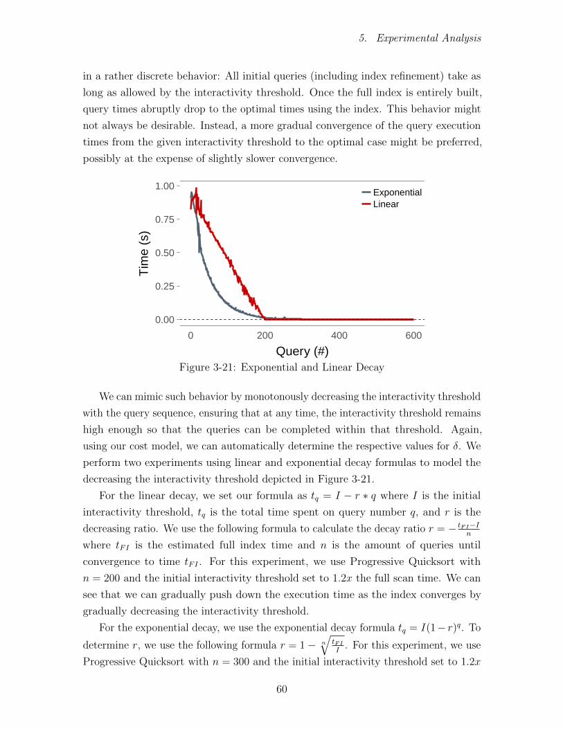
Figure 3-21: Exponential and Linear Decay

We can mimic such behavior by monotonously decreasing the interactivity threshold

with the query sequence, ensuring that at any time, the interactivity threshold remains

high enough so that the queries can be completed within that threshold. Again,

using our cost model, we can automatically determine the respective values for δ. We

perform two experiments using linear and exponential decay formulas to model the

decreasing the interactivity threshold depicted in Figure 3-21.

For the linear decay, we set our formula as tq = I − r ∗ q where I is the initial

interactivity threshold, tq is the total time spent on query number q, and r is the

decreasing ratio. We use the following formula to calculate the decay ratio r = − tFI−In

where tFI is the estimated full index time and n is the amount of queries until

convergence to time tFI . For this experiment, we use Progressive Quicksort with

n = 200 and the initial interactivity threshold set to 1.2x the full scan time. We can

see that we can gradually push down the execution time as the index converges by

gradually decreasing the interactivity threshold.

For the exponential decay, we use the exponential decay formula tq = I(1− r)q. To

determine r, we use the following formula r = 1− n

√tFII

. For this experiment, we use

Progressive Quicksort with n = 300 and the initial interactivity threshold set to 1.2x

60


the full scan time. Like the linear decay, we can see that the measured time closely

follows the interactivity threshold.

5.6 Adaptive Indexing Comparison

In this section, we will be comparing the greedy Progressive Indexing techniques with

existing Adaptive Indexing techniques. In particular, we focus on Standard Cracking

(STD), Stochastic Cracking (STC), progressive Stochastic Cracking (PSTC), Coarse

Granular Index (CGI), and Adaptive Adaptive Indexing (AA).

The implementations for the Full Index, Standard Cracking, Stochastic Cracking,

and Coarse Granular Index were inspired by the work done in Schuhknecht et al. [50]4.

The implementation for Progressive Stochastic Cracking was inspired by the work

done in Halim et al. [26]5. Progressive Stochastic Cracking is run with the allowed

swaps set to 10% of the base column. The implementation for the Adaptive Adaptive

Indexing algorithm has been provided to us by the authors of the Adaptive Adaptive

Indexing work [49], and we use the manual configuration suggested in their paper.

We compare all the Progressive Indexing techniques that we have introduced in

this work: Greedy Progressive Quicksort (PQ), Greedy Progressive Bucketsort (PB),

Greedy Progressive Radixsort LSD (PLSD), and Greedy Progressive Radixsort MSD

(PMSD). For each of the techniques, we use an adaptive indexing budget where we set

tbudget = 0.2 ∗ tscan, i.e., the cost of each query will be equivalent to 1.2 ∗ tscan until

convergence.

For reference, we also include the timing results when only performing full scans

on the data (FS) and when constructing a full index immediately on the first query

(FI). The full scan implementation uses predication to avoid branches, and the full

index bulk loads the data into a B+-tree, after which the B+-tree is used to answer

subsequent queries.

Metrics. The metrics that we are interested in are the time taken for the first

query, the number of queries required until convergence, the robustness of each of the

algorithms, and the cumulative response time. The robustness we compute by taking

the variance of the first 100 query times.

61


Table 3.2: SkyServer ResultsIndex First Q Convergence Robustness Cumulative

FS 0.75 x 0 118743.7FI 34.10 1 x 121.4

STD 5.26 x 0.290 1082.2STC 4.99 x 0.250 245.6

PSTC 4.89 x 0.240 254.5CGI 5.71 x 0.320 1008.9AA 8.50 x 0.800 188.4PQ 0.90 150 0.002 202.9

PMSD 0.90 119 0.030 157.5PLSD 0.81 368 3.4e-05 377.4

PB 0.83 138 0.009 166.4

SkyServer Workload

In this part of the experiments section, we execute the full SkyServer workload using

different indexing techniques. The results for each of the indexing techniques are

shown in Table 3.2. The algorithms have been divided into three sections: the baseline,

the Adaptive Indexing techniques, and the Progressive Indexing techniques.

The results for the baseline techniques are not very surprising. The full scan

method is the most robust, as we use predication, and no index is constructed. The

cost of each query is identical. The full scan method is also the cheapest method for the

first query’s cost as no time is spent on indexing at all. The full scan, however, takes

significantly longer to answer the full workload than the other methods. Answering

the full workload takes almost 30 hours, whereas all the other techniques finish the

entire workload under 20 minutes. The full index lies at the other extreme. It takes

50x longer to answer the first query while the index is being constructed. However, it

has the lowest cumulative time as the index can quickly answer all of the remaining

queries.

For the Adaptive Indexing techniques, we can see that their first query cost is

significantly lower than that of a full index but still significantly higher than that of a

full scan. Each of the Adaptive Indexing methods performs a significant amount of

work copying the data and cracking the index on the first query, resulting in a very

high cost for the first query. They do achieve a significantly faster cumulative time

than the full scans. However, in sum, they take longer than the full index to answer

the workload. Standard Cracking and Coarse Granular Indexing perform particularly

4https://infosys.uni-saarland.de/publications/uncracked_pieces_sourcecode.zip5https://github.com/felix-halim/scrack

62

https://infosys.uni-saarland.de/publications/uncracked_pieces_sourcecode.zip

https://github.com/felix-halim/scrack


poorly because of the workload’s sequential nature, as shown in Figure 3-9. Stochastic

Cracking and Adaptive Indexing perform better as they do not choose the pivots

based on the query predicates. Adaptive Adaptive Indexing has the best cumulative

performance, consistent with the results in Schuhknecht et al. [49].

The Progressive Indexing methods all have approximately the same cost for the

first query, which is 1.2x the scan cost. This is by design as we set the indexing

budget tbudget = 0.2 ∗ tscan for each of the algorithms. The main difference between

the algorithms is the robustness and the time until convergence. As we are executing

range queries, the Radixsort LSD performs the worst. The LSD partitioning cannot

help answer the range queries, and hence, the intermediate index does not speed up

the workload before convergence. Radixsort MSD performs the best, as the data set

is rather uniformly distributed. The radix partitioning works to efficiently create a

partitioning of the data, which can be immediately utilized to speed up subsequent

queries. For each of the Progressive Indexing methods, we see that they converge

relatively early in the workload. As we have set every query to take 1.2 ∗ tscan until

convergence, a significant amount of time can be spent on constructing the index for

each query, especially in later queries when the intermediate index can already be used

to obtain the answer efficiently. We also note that the Progressive Indexing methods

have a significantly higher robustness score than the Adaptive Indexing methods.

Progressive Indexing presents up to 4 orders of magnitude lower query variance when

compared to the Adaptive Indexing techniques. This is achieved by our cost model

balancing the per query execution cost to be (almost) the same until convergence,

while Adaptive Indexing suffers from many performance spikes.

●

Index (0.000003)

1.2x Scan (0.9)

10 1000

Query (#)

Que

ry T

ime

(log(

s))

● AA IdxP. QuickP. Stc 10%

Figure 3-22: Progressive Quicksort vs Adaptive Indexing. (all axes in log scale)

63


The execution time for each of the queries in the SkyServer workload is shown in

Figure 3-22. For clarity, we focus on the best Adaptive Indexing methods (Adaptive

Adaptive Indexing in terms of cumulative time, and Progressive Stochastic 10% in

terms of first query cost and robustness) and Progressive Quicksort. We can see

that both the Adaptive Indexing methods start with a significantly higher first query

cost and then fall quickly. Neither of them sufficiently converges, however, and both

continue to have many performance spikes. On the other hand, Progressive Quicksort

starts at the specified budget and maintains that query cost until convergence, after

which the cost drops to the cost of a full index.

Synthetic Workloads

In this part of our experiments, we execute all synthetic workloads described in

Section 5.1. All results are presented in tables. Each table is divided into four parts,

each representing one set of experiments. The first three are on data with 108 elements

and use random distribution, skewed distribution, and only point queries, respectively.

The final one is on 109 elements on random distribution. With the exception of point

queries and the ZoomIn and SeqZoomIn workloads, all queries have 0.1 selectivities.

From the Adaptive Indexing techniques, Adaptive Adaptive Indexing presents the

best cumulative time. Hence we select it for comparison. As previously, we set the

indexing budget tbudget = 0.2 ∗ tscan for each Progressive Indexing algorithm.

Table 3.3 depicts the cost of the first query for all algorithms. All Progressive

Indexing algorithms present a similar first query cost, which accounts for approximately

1.2x the scan cost, as chosen in our setup. Adaptive Indexing has a higher cost due to

the complete copy of the data and its full partition step in the first query. In general,

Progressive Indexing has one order of magnitude faster first query cost than Adaptive

Indexing.

Table 3.4 depicts the cumulative time of fully executing each workload. We can see

that Progressive Indexing outperforms Adaptive Indexing in most workloads under

uniform random data, except for the skewed and the periodic workload. This comes

with no surprise since Adaptive Indexing techniques have been designed to refine, and

boost access, to frequently accessed parts of the data. From the progressive algorithms,

radixsort (MSD) is the fastest since radixsort can outperform other techniques under

randomly distributed data.

For the skewed distribution, Adaptive Indexing outperforms Progressive Indexing

in almost all workloads due to its refinement strategy. However, Progressive Indexing

outperforms Adaptive Indexing for ZoomIn/Out workloads since each query accesses a

64


Table 3.3: First query costWorkload PQ PB PLSD PMSD AA

Uniform

Ran

dom

SeqOver 0.15 0.15 0.14 0.14 1.4ZoomOutAlt 0.15 0.15 0.14 0.14 1.4

Skew 0.15 0.15 0.14 0.14 1.4Random 0.15 0.15 0.14 0.14 1.4

SeqZoomIn 0.15 0.15 0.14 0.14 1.4Periodic 0.15 0.15 0.14 0.14 1.4

ZoomInAlt 0.15 0.15 0.14 0.14 1.4ZoomIn 0.15 0.15 0.14 0.14 1.4

Skewed


Skew 0.15 0.15 0.14 0.13 1.5Random 0.15 0.15 0.13 0.13 1.5



PointQuery


Skew 0.15 0.15 0.21 0.14 1.4Random 0.15 0.15 0.21 0.14 1.4Periodic 0.15 0.15 0.21 0.14 1.4

ZoomInAlt 0.15 0.15 0.21 0.14 1.4

109

SeqOver 1.5 1.5 1.4 1.7 13.9Skew 1.5 1.5 1.4 1.7 13.8

Random 1.5 1.5 1.4 1.7 25.4

different partition in different boundaries of the data, which leads to Adaptive Indexing

accessing large unrefined pieces in the initial queries. From the progressive algorithms,

bucketsort presents the fastest times since it generates equal-sized partitions for skewed

data distributions.

For point queries, radixsort (LSD) outperforms all algorithms in all workloads

since its intermediate index can be used early on to accelerate point queries.

Finally, for the 109 data size, Progressive Indexing manages to outperform adaptive

indexing even for the skewed workload. The key difference here is that the chunks

of unrefined data are bigger, and Progressive Indexing actually spends the time fully

converging them into small pieces. At the same time, Adaptive Indexing must manage

larger pieces of data.

Table 3.5 presents the robustness of the indexing algorithms. Progressive Indexing

presents up to four orders of magnitudes less variance than Adaptive Indexing. This is

due to the design characteristic of Progressive Indexing to inflict a controlled indexing

65

6. Summary

Table 3.4: Cumulative TimeWorkload PQ PB PLSD PMSD AA

Uniform

Random


Skew 18.8 17.7 48.1 15.9 10.1Random 24.7 22.8 53.1 21.1 29.1



Skewed


Skew 17.4 15.3 45.5 17.3 5.7Random 24.0 21.6 51.5 23.8 23.9



PointQuery


Skew 16.6 15.5 12.7 13.7 5.6Random 18.4 16.5 13.6 14.7 14.4Periodic 16.8 15.7 13.0 14.3 5.7

ZoomInAlt 17.7 15.9 13.2 14.1 15.2

109

SeqOver 516 493 924 480 653Skew 538 513 885 487 582

Random 773 718 1579 692 1104

penalty. For uniform random and skewed distributions, radixsort LSD presents the

least variance. This is due to the cost model noticing that the intermediate index

created by LSD cannot be used to boost query access, hence knowing the precise

cost of executing the query (i.e., a full scan cost). However, for point queries, the

intermediate index from LSD can already be used, which reduces the cost model

accuracy.

6 Summary

This chapter introduces Progressive Indexing, a novel incremental indexing technique

that offers robust and predictable query performance under different workloads. Pro-

gressive techniques perform indexing within an interactivity threshold and provide a

balance between fast convergence towards a full index together with a small perfor-

mance penalty for the initial queries. We propose four different Progressive Indexing

66


Table 3.5: RobustnessWorkload PQ PB PLSD PMSD AA

Uniform

Ran

dom

SeqOver 2.4e-04 5.8e-04 2.2e-05 2.1e-04 0.02ZoomOutAlt 1.7e-04 6.0e-04 2.1e-05 2.1e-04 0.02Skew 2.5e-04 6.2e-04 2.9e-05 2.3e-04 0.02Random 2.1e-04 6.5e-04 2.3e-05 2.0e-04 0.02SeqZoomIn 2.3e-04 5.5e-04 2.6e-05 2.1e-04 0.02Periodic 2.4e-04 6.6e-04 1.9e-05 2.1e-04 0.02ZoomInAlt 2.4e-04 5.4e-04 2.2e-05 2.1e-04 0.02ZoomIn 2.3e-04 3.8e-04 3.1e-05 1.4e-04 0.02

Skewed

SeqOver 3.7e-04 7.5e-04 1.6e-05 2.5e-03 0.03ZoomOutAlt 3.1e-04 7.6e-04 1.4e-05 2.7e-04 0.03Skew 3.5e-04 7.9e-04 1.4e-05 2.5e-03 0.03Random 3.4e-04 7.8e-04 1.9e-05 2.5e-03 0.03SeqZoomIn 3.6e-04 8.5e-04 1.4e-05 2.5e-03 0.03Periodic 3.2e-04 8.2e-04 1.5e-05 2.4e-03 0.03ZoomInAlt 3.4e-04 7.5e-04 1.4e-05 2.5e-03 0.02ZoomIn 1.9e-05 2.3e-04 1.4e-05 1.4e-03 0.02

PointQuery

SeqOver 2.4e-04 7.0e-04 1.5e-03 2.2e-04 0.02ZoomOutAlt 1.8e-04 6.3e-04 1.6e-03 2.1e-04 0.02Skew 2.6e-04 6.8e-04 1.6e-03 2.3e-04 0.02Random 2.2e-04 6.6e-04 1.6e-03 2.5e-04 0.02Periodic 2.2e-04 6.8e-04 1.1e-03 2.1e-04 0.02ZoomInAlt 2.3e-04 6.8e-04 1.5e-03 3.3e-04 0.02

109

SeqOver 0.02 0.03 2.8e-04 0.04 2.1Skew 8.1e-03 0.03 1.0e-04 0.03 2.1Random 0.01 0.03 2.4e-04 0.02 7.0

techniques and develop cost models for all of them that allow automatic tuning of

the budget. We show how they perform with both real and synthetic workloads

and compare their performance against Adaptive Indexing techniques. Based on

Figure 3-23: Progressive Indexing Decision Tree.

each algorithm’s main characteristics and the results of our experimental evaluation,

we conclude our work with the decision tree shown in Figure 3-23, which provides

recommendations on which technique to use in different situations. In this chapter,

we only present an algorithm to index unidimensional columns. However, queries

frequently have filters on multiple columns. In the next chapter, we will describe how

67

6. Summary

to create a Progressive Index that indexes multiple dimensions.

68

Progressive Indexes

Documents

Transcript of Progressive Indexes