Progressive Damage and Failure Analysis of Single Lap Shear and Double LapShear Bolted Joints

Ashith P. K. Joseph, Paul Davidson, Anthony M. Waas∗

William E Boeing Department of Aeronautics and Astronautics, University of Washington, 3940, Benton Ln NE, Seattle, WA, 98195

Abstract

Intra-inter crack band model (I2CBM) is proposed for studying the progressive damage and failure of laminatedcomposite bolted joints. The model combines Schapery theory for matrix microcrack modeling with crack band theoryfor lamina macroscopic failure modeling in a standard 3D finite element framework and is implemented as materiallaws at element integration points. Three different failure planes defined by material orthotropy are considered for themodeling of macroscopic failure using crack band theory. This procedure allows the model to be used either as anintraply element or as an interply element of finite thickness by an appropriate choice of the crack planes of interest.Localized bearing failure, observed in bolted joints, is modeled using a residual strength approach in the post-peakresponse of individual ply elements. Simulation results for single lap shear and double lap shear bolted joint problemsare compared against experiments for model validation.

Keywords:Composite laminates, Bolted joints, Progressive failure analysis, Virtual testing

1. Introduction

Even though composite material are finding increasing use in aviation and automotive sectors, bolted joints remainthe primary joining mechanism in most applications. Unlike bonding, bolted joints provide ease in maintainabilityand are less prone to failure due to manufacturing induced deviations from specifications. However, wherever there isa joint, bolted or bonded, it will likely be a site of damage and failure initiation in a structure. This is due to the fact5

that bolts require holes (or cut-outs) which act as a stress raiser within a structure. Hence, the need to properly sizethe bolted joint becomes of utmost concern in structural design.

Bolted joint analysis, using a computational framework, and that which is applicable for modern aerospace struc-tures, is a significant challenge owing to the complex nature of loading, and subsequent damage and response of thedamaged material[1, 2, 3, 4]. There are two parts to a bolt load, first the contact load on the hole inside surface, which10

is largely compressive. Second, the overall tensile load experienced by the bearing by-pass ligament. Hence, if onewere to isolate the failure regions, it would be the compressive/shear damage and failure due to the bolt contact loadand the tensile/shear damage and failure in the bypass ligament. There is however, significant interaction between thetwo regions, which can cause net section failure, shear-out failure, bearing failure or any combination of the above[5].15

Considerable literature is available which have identified the influencing parameters on failure of bolted joints.As with general application of laminated composites, bolt bearing strength is influenced by stack-up, hole size, ratioof hole diameter to width, ratio of hole diameter to free edge distance from hole center, in loading direction [6, 2].In addition, bearing strength of bolted joints is significantly influenced by clamp up load [7, 8, 9]. Higher clamp uploads tend to increase bearing strength, however it also can change the mode of failure. Clamp up loads introduce both20

∗Corresponding authorEmail address: awaas@aa.washington.edu (Anthony M. Waas)

Preprint submitted to Elsevier July 25, 2018

through thickness confinement of the composite, as well as friction. The process of bearing failure due to throughthickness confinement is well explained via experimental and microCT imaging by Xiao et al [10] and Wang et al [11].Their results show that bearing strength is influenced by the compressive strength of the 0◦ ply. Ultimate strength, onthe other hand, is due to much more complicated set of failure sequence. As the loading progresses, the 0◦ plies split,leading to failure in other off axis plies, which cause shear failure. Further loading induces bending of the undamaged25

ligament causing extensive delamination and 90◦ matrix failure. The complete two piece failure of a bolted joint hasalmost all possible failure modes associated with a composite material, making prediction using numerical methodschallenging.

Finite Element Analysis of bolted joint bearing strength prediction has been conducted in the past for pin loaded[12, 13] and bolted [14, 15, 16] composite lap joints. Both continuum damage and failure models [14] and Discrete30

failure models like XFEM [2] have been employed. Much of the past work has been concentrated on the predictionof bearing failure, however, as demonstrated by Crews [7], bearing failure and ultimate failure can differ quite sig-nificantly in magnitude especially under high bolt clamp up loads. Simulating progressive failure upto ultimate loadin a finite element framework, will require a model which captures in plane and out of plane failure modes and theinteraction of the two.35

In this study a new 3D Inter-Intra Crack Band Model (I2CBM) is proposed which can be used for modeling variousintraply and interply damage and failure mechanisms. In the next sections a detailed explanation of the I2CBM modelis provided, followed by numerical analysis and comparison of results for two bolted joint configurations, a DoubleLap Shear Bolted Joint (DLBJ) and a Single Lap Shear Bolted Joint (SLBJ).

2. Intra-inter Crack Band Model (I2CBM)40

The I2CBM [17, 18] is based on combining a pre-failure homogenized continuum model that includes distributedmicro-damage, with a post-peak equivalent continuum model that captures macro-cracks. Pre-peak lamina response,which dictates the overall composite material response is non-linear, especially in shear, owing to formation of microcracks in the matrix [19] (driven by local shear, figure 1). In I2CBM this nonlinearity is modeled using SchaperyTheory of micro damage [20]. Post-peak behavior, characterized by macroscopic fracture evolution is incorporated45

using crack band theory[21]. When an appropriate transition criterion is met (from pre-peak damage to post-peakfailure), post peak softening region begins and the area enclosed by the post peak response is the correspondingtoughness for that mode of failure, scaled by the element characteristic length [21, 22]. This toughness is mechanismdependent and coupon level testing is used to obtain the parameters that govern the individual toughness values.Alternatively, micromechanics modeling can be used to infer these values.50

Typical response of a stress-strain work conjugate pair implemented in I2CBM is shown in figure 1. As shownin the figure, at the lamina scale, damage is attributed to matrix microcracks and other sub-microcrack mechanismswhich are invisible to naked eye, but that which contributed to dissipation leading to nonlinearity in observed couponlevel testing, such as reported in [19]. Notice that the tangent stiffness of the stress-strain response is positive duringdamage evolution and the material is assumed be in continuum state. The energy dissipated in microcrack formation55

is denoted by S as shown in figure 1. Failure is defined by a transition criterion and corresponds to a macroscopicevent. For instance, in predominantly tensile stress states, microcracks coalesce to form a macrocrack. Macrocrackformation releases energy corresponding to the toughness of that particular failure mode. In addition to the abovefeature, additional important characteristics of the I2CBM model are as follows;

1. A single type of 3D finite element is used seamlessly throughout an analysis for both intra-ply and inter-ply60

modeling. 2. A coupled failure mechanism which links in-plane (intra-ply) failure to inter-ply (delamination) failureis used. This is based on the experimental observation that shows during in-plane loading of laminates, delaminationdue to failure of interface layer between two plies can only initiate if an intralaminar macrocrack forms within one ofthe plies. However this feature is not used when the ply elements experience out-of-plane compressive stresses andhence not relevant for bolted joint problems analyzed here. 3. To ensure correct energy dissipation during the post-65

peak regime and under mixed-mode conditions, the normal and shear surface tractions must vanish simultaneouslyat failure through cracking since a crack must have zero tractions on its surface. A novel incremental mixed modeevolution law has been implemented to achieve this[17, 18]. 4. The strength values are statistically distributed overthe geometry of the test coupon. This approach takes the strength variation measured in the experiments, and helps tomodel localization of failure events and is representative of the physical nature of material strength (it is not constant70

2

throughout a volume). 5. For compressive mechanisms of failure, residual strength approach is used to account forpost-kink banding strength retention under confined compression of zero degree plies. When the residual compressivestrength level is reached, the stress state is fixed at that value for further increments of loading in the post-peakregime. The value of the residual strength is dependent on the material and can be affected by geometric featuressuch as spatial constraints and bolt pretension. 6. Accurate calculation of element characteristic length for various75

failure modes. Since I2CBM is implemented as a user subroutine in the commercial finite element code, the averagecharacteristic lengths provided by the FE solver need not be correct and can lead to incorrect energy dissipation. Thecorrect characteristic lengths for each mode is calculated separately. 7. A global crack spacing method is used forintralaminar macro-cracking, ensuring that a certain spacing is maintained between adjacent cracks as observed inexperiments[17, 18].80

Damage : Continuum

Failure : Non-continuum

(a) Damage – Micro cracks

(c) Damage - Schematic

(e) Damage – DIC Image (f) Failure – DIC Image

(d) Failure – Schematic

(b) Failure –Macro cracks

Figure 1: Generalized stress-strain response for damage and failure events. (a) Microcracks developed in ± 45◦ tension test specimen [19]. (b)Macrocracks in ± 45◦ tension test specimen. (c) & (d) Schematic showing transition from damage to failure state. (e) & (f) DIC images showingthe transition from damage to failure state

3

2.1. Schapery Theory for 3D Stress State

Schapery theory (ST) is an energy based approach for modeling the transverse and shear moduli of homogenizedlaminae that degrade due to the development of matrix microcracks prior to the attainment of a peak stress state[20, 23, 22]. ST characterizes the non-linear matrix dominated responses as a function of the energy dissipated duringthe microcrack formation. It is also assumed that the fiber direction stiffness is unaffected by the microcrack formation85

as the fiber stiffness is much larger than matrix stiffness. In I2CBM, ST is extended from a plane stress state to 3Dstates of stress as shown in this paper. Transverse and shear moduli degradations with microcracks are modeled usingfunctions es and gs respectively as shown in equation 1 and they are functions of the energy dissipated (S) due tomatrix microcrack formation[20, 23, 22]. 2D Schapery Theory[20, 23, 22] is extended to model 3D stress states asdescribed below.90

E22 = E220es(S )G12 = G120gs(S ) (1)

Where E220 and G120 represent the initial lamina transverse and shear stiffness values respectively. Schaperymicrodamage functions es and gs are generally expressed as fifth order polynomial functions as shown in [20, 23, 22].

With the transversely isotropic assumption of the lamina, out of plane stiffness properties are degraded as shownbelow.

E33 = E220es(S )G13 = G120gs(S )G23 = G230es(S )

(2)

where E230 is the initial lamina shear stiffness in the 2-3 plane of transverse isotropy.95

The total energy of an element in the microdamaged state can be written as a sum of the elastic and microdamageenergies as below

WT = WE + S (3)

Where WT , WE and S are total energy, elastic energy and energy dissipated due to microdamage respectively.Following the procedure used in 2D Schapery theory[20, 23, 22], microdamage evolution equation can be obtainedusing the condition that the total energy is stationary with respect to microdamage energy Sr = S 1/3. Equation 4 can be100

solved at any given state to estimate microdamage energy S and can be substituted into equations 1 and 2 to calculatethe current material stiffness properties.

[2(ν12 + ν12ν23)ε11ε22 + 2(ν23 + ν12ν21)ε22ε33 + 2(ν12 + ν12ν23)ε11ε33

+(1 − ν12ν21)ε222 + (1 − ν12ν21)ε2

33] E220∆

desdS r

+G230γ223

desdS r

+ G012(γ2

12 + γ213) dgs

dS r= −6S 2

r

(4)

Where ∆ = (1 − 2ν12ν21 − ν23ν23 − 2ν12ν21ν23)

4

2.2. Crack Band Theory

E*

cG

δ = le*εcr

+ =

c

e

G

l

E*

ε

σC

εel

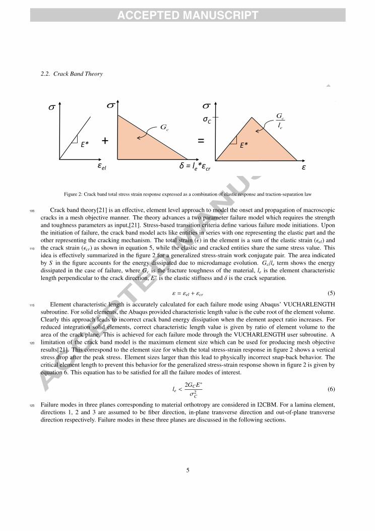
Figure 2: Crack band total stress strain response expressed as a combination of elastic response and traction-separation law

Crack band theory[21] is an effective, element level approach to model the onset and propagation of macroscopic105

cracks in a mesh objective manner. The theory advances a two parameter failure model which requires the strengthand toughness parameters as input,[21]. Stress-based transition criteria define various failure mode initiations. Uponthe initiation of failure, the crack band model acts like entities in series with one representing the elastic part and theother representing the cracking mechanism. The total strain (ε) in the element is a sum of the elastic strain (εel) andthe crack strain (εcr) as shown in equation 5, while the elastic and cracked entities share the same stress value. This110

idea is effectively summarized in the figure 2 for a generalized stress-strain work conjugate pair. The area indicatedby S in the figure accounts for the energy dissipated due to microdamage evolution. Gc/le term shows the energydissipated in the case of failure, where Gc is the fracture toughness of the material, le is the element characteristiclength perpendicular to the crack direction, E∗ is the elastic stiffness and δ is the crack separation.

ε = εel + εcr (5)

Element characteristic length is accurately calculated for each failure mode using Abaqus’ VUCHARLENGTH115

subroutine. For solid elements, the Abaqus provided characteristic length value is the cube root of the element volume.Clearly this approach leads to incorrect crack band energy dissipation when the element aspect ratio increases. Forreduced integration solid elements, correct characteristic length value is given by ratio of element volume to thearea of the crack plane. This is achieved for each failure mode through the VUCHARLENGTH user subroutine. Alimitation of the crack band model is the maximum element size which can be used for producing mesh objective120

results[21]. This correspond to the element size for which the total stress-strain response in figure 2 shows a verticalstress drop after the peak stress. Element sizes larger than this lead to physically incorrect snap-back behavior. Thecritical element length to prevent this behavior for the generalized stress-strain response shown in figure 2 is given byequation 6. This equation has to be satisfied for all the failure modes of interest.

le <2GC E∗

σ2C

(6)

Failure modes in three planes corresponding to material orthotropy are considered in I2CBM. For a lamina element,125

directions 1, 2 and 3 are assumed to be fiber direction, in-plane transverse direction and out-of-plane transversedirection respectively. Failure modes in these three planes are discussed in the following sections.

5

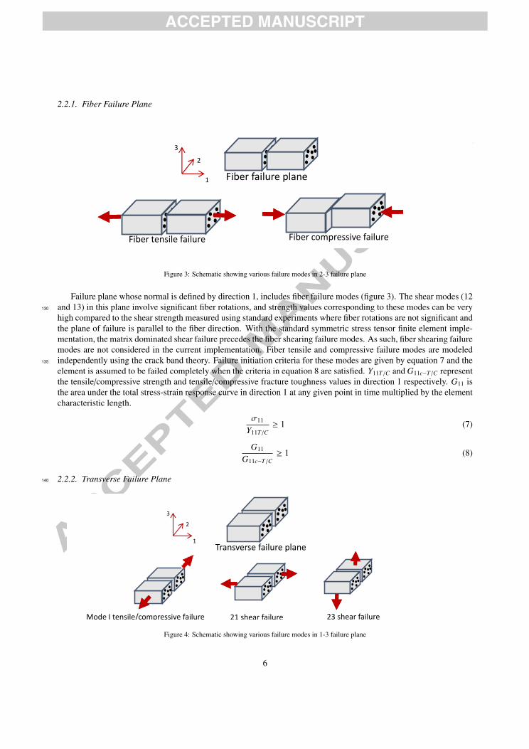
2.2.1. Fiber Failure Plane

Fiber failure plane

Fiber tensile failure Fiber compressive failure

2

3

1

Figure 3: Schematic showing various failure modes in 2-3 failure plane

Failure plane whose normal is defined by direction 1, includes fiber failure modes (figure 3). The shear modes (12and 13) in this plane involve significant fiber rotations, and strength values corresponding to these modes can be very130

high compared to the shear strength measured using standard experiments where fiber rotations are not significant andthe plane of failure is parallel to the fiber direction. With the standard symmetric stress tensor finite element imple-mentation, the matrix dominated shear failure precedes the fiber shearing failure modes. As such, fiber shearing failuremodes are not considered in the current implementation. Fiber tensile and compressive failure modes are modeledindependently using the crack band theory. Failure initiation criteria for these modes are given by equation 7 and the135

element is assumed to be failed completely when the criteria in equation 8 are satisfied. Y11T/C and G11c−T/C representthe tensile/compressive strength and tensile/compressive fracture toughness values in direction 1 respectively. G11 isthe area under the total stress-strain response curve in direction 1 at any given point in time multiplied by the elementcharacteristic length.

σ11

Y11T/C≥ 1 (7)

G11

G11c−T/C≥ 1 (8)

2.2.2. Transverse Failure Plane140

2

3

1Transverse failure plane

21 shear failure 23 shear failureMode I tensile/compressive failure

Figure 4: Schematic showing various failure modes in 1-3 failure plane

6

Transverse failure modes shown in figure 4 are characterized by macro cracks in the matrix and hence appropriatemixed mode laws are to be used in modeling these. A quadratic mixed mode criterion is used for failure initiationunder the general combined loading situation and it is given by equation 9. Y22T/C , S 12 and S 23 are tensile/compressivestrength in direction 2, 12 shear strength and 23 shear strength respectively.

σ222

Y222T/C

+τ2

12S 2

12+

τ223

S 223≥ 1 (9)

Mixed mode evolution criterion given by equation 10 is used to determine the completely failed state. G22c−T/C ,145

G12c and G23c are tensile/compressive fracture toughness in direction 2, 12 shear fracture toughness and 23 shearfracture toughness values respectively. G22, G12 and G23 are areas under the individual mode total stress-strain re-sponse curves at any given point in time multiplied by the element characteristic length. An incremental mixed modeevolution law as described in [17, 18] is used to ensure that the tractions at the failure plane vanish simultaneouslywhen equation 10 is satisfied.150

G22G22c−T/C

+ G12G12c

+G23G23c≥ 1

(10)

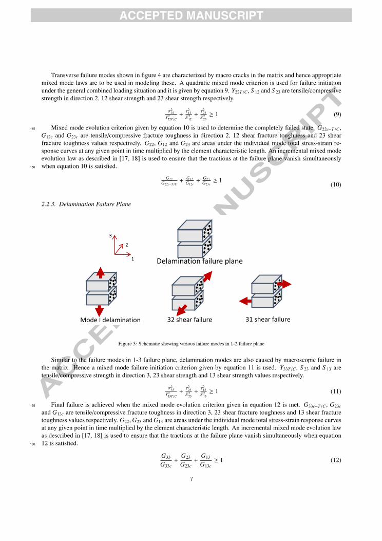
2.2.3. Delamination Failure Plane

2

3

1

Mode I delamination 32 shear failure 31 shear failure

Delamination failure plane

Figure 5: Schematic showing various failure modes in 1-2 failure plane

Similar to the failure modes in 1-3 failure plane, delamination modes are also caused by macroscopic failure inthe matrix. Hence a mixed mode failure initiation criterion given by equation 11 is used. Y33T/C , S 23 and S 13 aretensile/compressive strength in direction 3, 23 shear strength and 13 shear strength values respectively.

σ233

Y233T/C

+τ2

23

S 223

+τ2

13

S 213≥ 1 (11)

Final failure is achieved when the mixed mode evolution criterion given in equation 12 is met. G33c−T/C , G23c155

and G13c are tensile/compressive fracture toughness in direction 3, 23 shear fracture toughness and 13 shear fracturetoughness values respectively. G22, G23 and G13 are areas under the individual mode total stress-strain response curvesat any given point in time multiplied by the element characteristic length. An incremental mixed mode evolution lawas described in [17, 18] is used to ensure that the tractions at the failure plane vanish simultaneously when equation12 is satisfied.160

G33

G33c+

G23

G23c+

G13

G13c≥ 1 (12)

7

A delamination element can be created by disabling fiber and transverse failure planes. For the matrix rich interfaceelements used in this study, only delamination failure plane is activated.

2.2.4. Failure Plane InteractionsMultiple failure planes/modes can coexist in the same element. Transverse and delamination failure modes are

linked to each other as both are associated with matrix cracks. Therefore initiation of one of those failure planes165

causes the initiation in other failure plane as well. The fiber mode is treated independent of the other modes. Thestiffness matrix is treated as a diagonal matrix when any of the transition criteria is met. This is different from thestandard implementation of crack band/smeared crack model which has off diagonal terms in the stiffness matrix postfailure initiation. In I2CBM, it is assumed that post failure initiation, material is in a non-continuum state and Poissonseffects in this state are not considered. However diagonal terms are updated at failure initiation to preserve the energy170

during the stiffness matrix diagonalization process. This also simplifies the implementation of the crack band theoryas the stress-strain responses of failure modes become independent of each other but subjected to the conditions of theincremental mixed mode evolution law.

2.3. Modeling of Bearing FailureFiber kinking is an instability facilitated by the non-linear shear response of the matrix. Since compressive failure175

through fiber kinking is one of the key mechanisms in the failure analysis of bolted joints, modifications have beenmade to implement this failure mode to account for the effect of bolt pretension and other spatial constraints. Fiberkinking instability is influenced by the 3D state of stress. Significant compressive stresses in the transverse and outof plane directions can potentially stabilize the non-linear shear response and increase the effective fiber compressivestrength. While this is an area which requires more research, a simplified approach is taken in this analysis to capture180

the effects of spatial constraints on kink banding and multiple kink band mechanism observed in experiments[10].

(a)

(b)

Figure 6: (a) Cross section view of a double lap shear bolted joint configuration. (b) Multiple kink band formation in the bearing region[10]

8

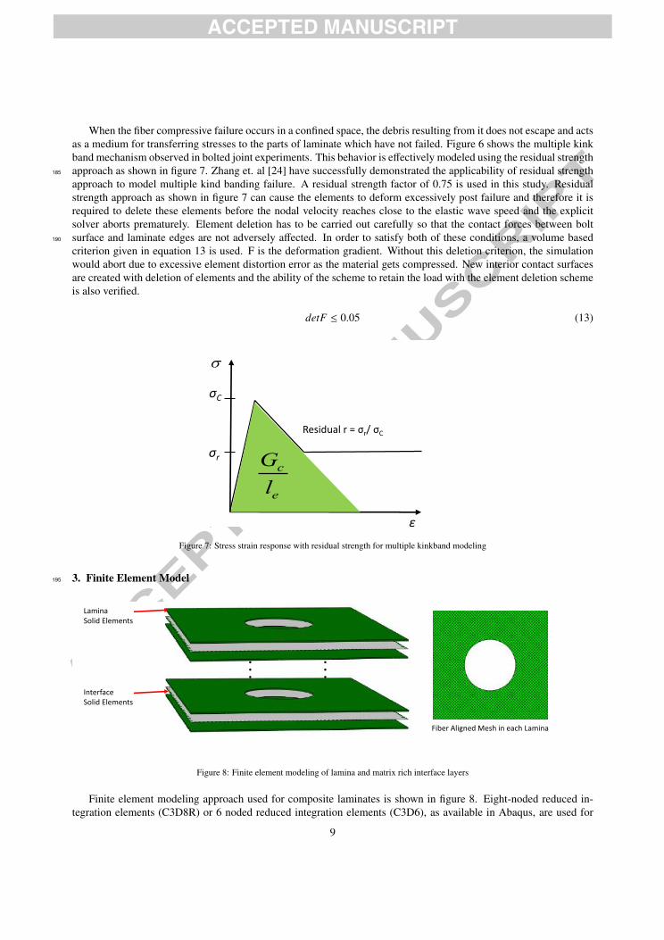
When the fiber compressive failure occurs in a confined space, the debris resulting from it does not escape and actsas a medium for transferring stresses to the parts of laminate which have not failed. Figure 6 shows the multiple kinkband mechanism observed in bolted joint experiments. This behavior is effectively modeled using the residual strengthapproach as shown in figure 7. Zhang et. al [24] have successfully demonstrated the applicability of residual strength185

approach to model multiple kind banding failure. A residual strength factor of 0.75 is used in this study. Residualstrength approach as shown in figure 7 can cause the elements to deform excessively post failure and therefore it isrequired to delete these elements before the nodal velocity reaches close to the elastic wave speed and the explicitsolver aborts prematurely. Element deletion has to be carried out carefully so that the contact forces between boltsurface and laminate edges are not adversely affected. In order to satisfy both of these conditions, a volume based190

criterion given in equation 13 is used. F is the deformation gradient. Without this deletion criterion, the simulationwould abort due to excessive element distortion error as the material gets compressed. New interior contact surfacesare created with deletion of elements and the ability of the scheme to retain the load with the element deletion schemeis also verified.

detF ≤ 0.05 (13)

ε

σC

σrc

e

G

l

Residual r = σr/ σC

Figure 7: Stress strain response with residual strength for multiple kinkband modeling

3. Finite Element Model195

. .. .. .

LaminaSolid Elements

InterfaceSolid Elements

Fiber Aligned Mesh in each Lamina

Figure 8: Finite element modeling of lamina and matrix rich interface layers

Finite element modeling approach used for composite laminates is shown in figure 8. Eight-noded reduced in-tegration elements (C3D8R) or 6 noded reduced integration elements (C3D6), as available in Abaqus, are used for

9

all the lamina and interface layers. Each lamina and matrix rich interface layers are modeled separately and they areconnected using node to surface tie commands. I2CBM material formulation is used for both lamina and matrix richinterface elements. Delamination failure plane is the only active failure plane in matrix rich interface elements. Matrix200

rich interface layer is assumed to have a thickness value corresponding to 10% of the lamina thickness based on themicroscopic images of similar carbon fiber epoxy unidirectional tape laminates. Total thickness of the laminates aremaintained in this process and the stiffness properties of the lamina layers are scaled up accordingly to maintain theexact laminate stiffness. The element size is kept as 0.01 in the region of interest. The element sizes were chosen suchthat stress convergence and crack band characteristic length restrictions are satisfied.205

Fiber aligned meshes are used for modeling each lamina layer and this is achieved using an in-house developedfiber aligned meshing tool. Stress contour around a degraded element depends on the finite element discretizationaround it and not paying attention to this may produce unexpected bias in the subsequent failure events. While materialproperties in the homogenized elements are orthotropic in nature, it is more sensible to have the nodes also alignedalong the principal material (orthotropic) planes. These issues are often seen in problems where shear cracks grow210

parallel to the fiber direction. An unstructured mesh with the same level of mesh density may lead to incorrect failurepatterns, however, as the mesh gets refined, discretization related issues even with an unstructured mesh diminish,[22].

Commercially available meshing tools do not provide any option for generating fiber aligned meshes and a skilleduser has to rely on partitioning the geometry in smart ways to achieve this. However this often leads to bad element215

definitions near the geometric discontinuities such as a hole. The present fiber aligned mesh generation tool helpsin overcoming these difficulties and generates a mesh compatible with Abaqus FE solver. It can generate the meshfor each ply in a composite as per the fiber alignment, with perfect displacement continuity between layers (as inthe ABAQUS tie command). This is a Matlab based tool which needs only a minimum number of inputs for themesh generation and can handle geometric discontinuities such as countersunk holes. A combination of 8 noded and220

6 noded Abaqus 3D elements are used for capturing geometric discontinuities and also ensures the quality of theelements. A mesh transition feature is also used which can make the mesh coarser away from the region of interestand reduce the computational cost.

All the analyses are performed using the commercial software, Abaqus, using an explicit method. Linear elasticanalysis was carried out as the initial step to ensure that the ratio of kinetic energy to internal energy is kept below 5%225

for the loading rates and mass scaling values chosen. Explicit analysis time can be reduced either by increasing theloading rate or by using mass scaling approach. A loading rate of 0.10in/s is used for all the simulations presentedhere. Variable mass scaling option in Abaqus is used with the minimum time increment value of 5e-6s.

DLBJ and SLBJ tests were conducted for a generic 36 ply composite laminate with hole diameter (D) of 0.25”.Both specimens have a specimen width to diameter (W/D) ratio of 6 and edge distance of 1.5*D. Composite laminate230

were modeled using a layer-by-layer approach where each layer of the composite ply and matrix layer is modeledexplicitly. Laminate was design for a 44% - 0◦, 44% - ± 45◦ and 12% - 90◦ plies.

To reduce the model size, a refined fiber aligned mesh region was generated around the bolt (figure 9,10). Themesh size in this region follows Bazant’s criteria [21] which provides an upper limit to the mesh size for a givenenergy release rate. The fine region is smoothly transitioned to the coarse region.235

The complete bolted joint analysis is conducted using ABAQUS explicit. It is a two-step analysis where the firststep is to simulate bolt pre-tension load and the second, the progressive failure. Bolt pre-tension load is introducedby conducting a thermal analysis of the bolt [25]. With initial temperature of the bolt shank kept at zero degrees K,a negative temperature boundary condition was applied on the bolt shank. Material thermal properties were modifiedsuch that the bolt shank contracts only in the axial direction, hence inducing bolt pre-tension. Bolt pretension value240

for the results presented here is 500lbs.General contact algorithm is used for all interface regions. An erosion set is defined for the fine mesh region where

the bolt is expected to elongate and erode the mesh. By defining an erosion set and defining internal surfaces, the codeis able to re-generate the contact surfaces as the elements are eroded. Thus, ensuring force transfer as the elementsget deleted.245

In DLBJ, composite specimen is bolted between two steel reaction skins. FEM model for DLBJ is shown in figure9, Here, relative displacement measurements are made with an extensometer attached to the steel plates and compositetest specimen, while the loading is applied in a load-controlled setting. SLBJ has a countersunk hole and bolted to asteel plate. The specimen was loaded and then unloaded in displacement control loading. The dimensions, mesh and

10

boundary conditions are shown in figure 10.250

Experimental results found in the literature show the absence of delamination in the region where the effect of boltpretension is transferred to the specimen[10]. Hence intra-inter communication is disabled in the region under thewasher and the delamination strength values are set high to prevent it’s occurrence. It was observed in the simulationthat the premature delamination failure near the hole reduces the effectiveness of modeling bearing failure usingresidual strength state. Correct delamination strength values and intra-inter communication are used in all the other255

regions for effectively capturing the final two-piece failure mechanism.

P

Composite testspecimen

Reaction skin

Spacer

Extensometercross brace

BoltCollar

NutFiber aligned refined mesh

Fiber aligned refined mesh

Figure 9: Double Lap Shear Bolted Joint model

Composite testspecimen

Nut

Counter sunk bolt

Fiber aligned refined mesh

Fiber aligned refined mesh

Figure 10: Single Lap Shear Bolted Joint model

11

Input material data used in the simulation is given in table 1. Transverse isotropy assumption is used here for allthe material parameters. Test and inverse analysis methods used for determining the input parameters are also addedin the table. Matrix rich interface layer is assumed to have the same stiffness, strength and toughness properties as thelamina transverse direction.260

Property Recommended Test

Lamina Properties

E11 [90°/0°]s Tension Test

E22 90° Tension Test

ν12 0° Tension Test

G12 ±45° Tension Test

Failure Properties

Y11𝑇 [90°/0°]s Tension Test

Y11𝐶 [90°/0°]s Compression Test/ Predicted for 1.2° fibermisalignment using shear non-linear response data

Y22𝑇 90° Tension Test

Y22𝐶 90° Compression Test

𝑆12 ±45° Tension Test

Fracture Toughness

𝐺11𝑐−𝑇/𝐶 Inverse FE analysis of open hole tension/compression

𝐺22𝑐−𝑇/𝐶 DCB Test

𝐺12𝑐 ENF Test

Table 1: Material properties needed and suggested tests/inverse analysis method to obtain them

4. Results and Discussion

Load-displacement response of the DLBJ is compared against experimental data in figure 11. Extensometerdisplacement δ as shown in figure 9 is plotted against the applied load in figure 11. The initial non-linearity inthe simulation response indicated as point A, is caused by the bearing failure and the section view of the failurepattern at that point is also shown in figure 11. The failure pattern in various layers at the bearing load is shown in265

figure 12. Splitting cracks in the 0 layer and shear cracks tangent to the hole in the 45 layer are dominant. Also,the fiber failure regions are localized in each ply according to fiber orientation. The reason for the error in the initialstiffness in the simulation is unknown and it is possibly caused by uncertainty in experimental measurements includingthe extensometer measurements and/or uncertainty in in-situ lamina elastic properties. Similar to the experiment,simulation was carried out using load controlled boundary conditions. Failure events in the post peak region are270

catastrophic and dynamic in nature due to the load controlled boundary condition.

12

Bearing Failure

Final Failure

A

B

AB

Matrix Failure

Fiber Failure

Matrix Failure

Fiber Failure

Undamaged

Post Peak Softening (Failure Initiation)

Residual State/Failed

Figure 11: Load-displacement repsonse of double lap shear bolted joint and bearing failure status at critical points

Figure 13 compares the final failure pattern in the simulation with the failed specimen. Failed specimens showpredominantly bearing and tear out failure mechanisms. Simulations are able to go through catastrophic failure eventswithout losing the contact forces due to the bearing failure model described in section 2.3. Stress concentrationscreated by the change in mesh size act as the point at which final two piece failure occurs. The deletion scheme used275

in the simulation removes the elements undergoing excessive distortion and hence is not shown in the images. Themodel could not capture some of the delamination and 90 layer transverse crack failure mechanisms shown in thefigure and it can be attributed to the dynamic nature of the failure events. The model showed negligible yielding inthe bolt and the same was observed in the experiments.

Mat

rix

Failu

reFi

ber

Fai

lure

Layer 1 (45) Layer 8 (90) Layer 15 (-45) Layer 17 (0)

Undamaged

Post Peak Softening (Failure Initiation)

Residual State/Failed

Figure 12: Lamina failure pattern in double lap shear bolted joint at bearing load (Point A in figure 11)

13

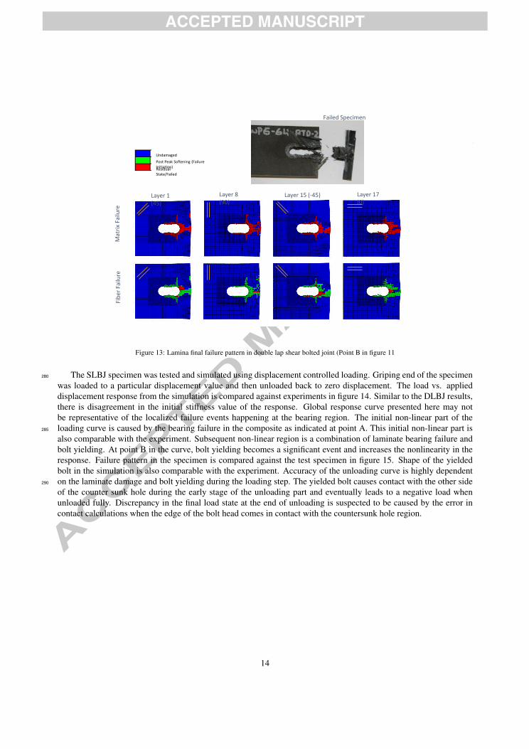
Mat

rix

Failu

reFi

ber

Fai

lure

Failed Specimen

Layer 1 (45)

Layer 8 (90)

Layer 15 (-45) Layer 17 (0)

Undamaged

Post Peak Softening (Failure Initiation)Residual State/Failed

Figure 13: Lamina final failure pattern in double lap shear bolted joint (Point B in figure 11

The SLBJ specimen was tested and simulated using displacement controlled loading. Griping end of the specimen280

was loaded to a particular displacement value and then unloaded back to zero displacement. The load vs. applieddisplacement response from the simulation is compared against experiments in figure 14. Similar to the DLBJ results,there is disagreement in the initial stiffness value of the response. Global response curve presented here may notbe representative of the localized failure events happening at the bearing region. The initial non-linear part of theloading curve is caused by the bearing failure in the composite as indicated at point A. This initial non-linear part is285

also comparable with the experiment. Subsequent non-linear region is a combination of laminate bearing failure andbolt yielding. At point B in the curve, bolt yielding becomes a significant event and increases the nonlinearity in theresponse. Failure pattern in the specimen is compared against the test specimen in figure 15. Shape of the yieldedbolt in the simulation is also comparable with the experiment. Accuracy of the unloading curve is highly dependenton the laminate damage and bolt yielding during the loading step. The yielded bolt causes contact with the other side290

of the counter sunk hole during the early stage of the unloading part and eventually leads to a negative load whenunloaded fully. Discrepancy in the final load state at the end of unloading is suspected to be caused by the error incontact calculations when the edge of the bolt head comes in contact with the countersunk hole region.

14