Programming with SPSS Syntax and Macros - ncids.org evaluation...
154
Programming with SPSS Syntax and Macros SPSS Inc. 233 S Wacker Drive, 11th Floor Chicago, Illinois 60606 312.651.3000 Training Department 800.543.6607 v10.0 Revised 12/31/99 ss
Transcript of Programming with SPSS Syntax and Macros - ncids.org evaluation...

Programming with SPSSSyntax and Macros
SPSS Inc.233 S Wacker Drive, 11th FloorChicago, Illinois 60606312.651.3000
Training Department800.543.6607
v10.0 Revised 12/31/99 ss

SPSS Neural Connection, SPSS QI Analyst, SPSS for Windows, SPSS DataEntry II, SPSS-X, SCSS, SPSS/PC, SPSS/PC+, SPSS Categories, SPSS Graphics,SPSS Professional Statistics, SPSS Advanced Statistics, SPSS Tables, SPSSTrends, SPSS Exact Tests, and SPSS Missing Value are the trademarks of SPSSInc. for its proprietary computer software. CHAID for Windows is the trademarkof SPSS Inc. and Statistical Innovations Inc. for its proprietary computersoftware. Excel for Windows and Word for Windows are trademarks of Microsoft;dBase is a trademark of Borland; Lotus 1-2-3 is a trademark of LotusDevelopment Corp. No material describing such software may be produced ordistributed without the written permission of the owners of the trademark andlicense rights in the software and the copyrights in the published materials.
General notice: Other product names mentioned herein are used foridentification purposes only and may be trademarks of their respectivecompanies.
Copyright(c) 2000 by SPSS Inc.
All rights reserved.
Printed in the United States of America.
No part of this publication may be reproduced or distributed in any form or byany means, or stored on a database or retrieval system, without the prior writtenpermission of the publisher, except as permitted under the United StatesCopyright Act of 1976.

Table of Contents - 1
SPSS Training
Programming with SPSS Syntax and MacrosTable of Contents
Introduction and Syntax ReviewA Data Manipulation Example 1 - 1A Macro Example 1 - 3Rules and Aids for SPSS Syntax 1 - 6Advice for Those Working with Syntax 1 - 9Summary 1-10
Basic SPSS Programming ConceptsCommand Types in SPSS 2 - 2The Three Types of SPSS Programming 2 - 3SPSS Data Definition 2 - 5SPSS Programming Constructs 2 - 6Do If & End If 2 - 6Do Repeat & End Repeat 2 - 7Loop & End Loop 2 - 9Scratch Variables 2-11Vector 2-12Summary 2-16
Complex File TypesASCII Data and Records 3 - 2File Types 3 - 2Syntax Basics 3 - 3Data File Structure 3 - 4Grouped Data 3 - 4Mixed Data 3 - 5Nested Data 3 - 6Reading a Mixed File 3 - 7Errors in the Data 3-10Grouped File Type Without Record Information 3-12Summary 3-17
Input ProgramsSyntax Components 4 - 2Example 1: Change the Case Base of a File 4 - 2End of Case Processing 4 - 7End of File Processing 4 - 9Checking Input Programs 4-10Incomplete Input Programs 4-11
Chapter 1
Chapter 3
Chapter 2
Chapter 4

SPSS Training
Table of Contents - 2
Exercises
Example 2: Reading Files with Missing Identifiers 4-14When Things Go Wrong 4-20Summary 4-21
Advanced Data ManipulationReading a Comma-Delimited File 5 - 2Reading Multiple Cases on the Same Record 5 - 7An Existing SPSS Data File with Repeating Data 5-11Print Command for Diagnostics 5-15Practical Example: Consolidating Transactions 5-17Summary 5-24Appendix: Identifying Missing Values by Case 5-25
Introduction to MacrosMacro Basics 6 - 2Macro Arguments 6 - 3Macro Tokens 6 - 3Viewing a Macro Expansion 6 - 7Keyword Arguments 6 - 8Using a Varying Number of Tokens 6-10When Things Go Wrong 6-15Summary 6-18
Advanced MacrosLooping in Macros 7 - 2Producing Several Clustered Bar Charts 7 - 2Double Loops in Macros 7 - 5String Manipulation Functions 7 - 7Direct Assignment of Macro Variables 7 - 7Conditional Processing 7 - 7Creating Concatenated Stub and Banner Tables 7 - 8Additional Recommendations 7-13Summary 7-13
Macro TricksCombining Input Programs and Macros 8 - 2Ordering Tables and Charts 8 - 6The Case of the Disappearing Command 8 - 9Summary 8-14
ExercisesExercises E - 1
Chapter 6
Chapter 7
Chapter 8
Chapter 5

Introduction and Syntax Review 1 - 1
SPSS Training
Introduction and SyntaxReview
A Data Manipulation ExampleA Macro ExampleRules and Aids for SPSS SyntaxAdvice for Those Working with Syntax
This course has two major topical areas. We will review how to useSPSS Syntax to perform complex data manipulations that are notavailable under the SPSS menu system. This will be of interest to
those who need to read complex data files from legacy computer systems(for example, legacy health care data, transaction oriented sales systems)and those who find they need to reorganize their data in order to performa desired analysis. Examples of the latter include marketing andcustomer relationship studies in which a number of products (or servicesof an company) are rated on each of many attributes. All informationfrom a respondent is typically stored in a single record, but needs to bespread across multiple records in order for factor analysis and perceptualmapping to be performed. When preparing data for churn (customerretention – for telecoms, credit card issuers, insurance companies)studies, comparisons might need to be made across transactional recordssorted by customer ID and date. SPSS Syntax permits a richer array ofdata manipulations in this content than would the menu system. Inshort, we will examine uses of SPSS Syntax to facilitate analysis of fileswith complex structures or files that must be restructured for a desiredanalysis.
The second topical area concerns automation in SPSS through theSPSS macro language. SPSS macros can generate SPSS Syntax, which isthen executed. For this reason, macros are very handy in situationswhere SPSS Syntax needs to be run repeatedly, but with minor andsystematic changes each time. For example, you might wish to producethirty Interactive graphs, each a clustered bar chart containing ademographic variable and one of thirty rating scale variables. Within theSPSS menu system, changes would have to be made in the Interactivegraph dialog box for each graph. Instead, an SPSS macro could generatethe SPSS Syntax for each interactive graph within a loop, substituting anew rating scale variable name per iteration. In this way, the SPSSmacro language can automate what would otherwise be time-consumingtasks for the analyst.
Chapter 1
Topics
INTRODUCTION

SPSS Training
Introduction and Syntax Review 1 - 2
Since these topics involve SPSS Syntax, we will use the dialog boxeswithin SPSS infrequently. A prerequisite for this course is familiaritywith SPSS Syntax at the level of our Introduction to SPSS Syntaxtraining course. In this chapter, we will present a sample of datamanipulation with SPSS syntax and a macro example, and provide abrief review of and some recommendations for SPSS Syntax.
To illustrate the type of data manipulation that can be performed withSPSS Syntax, we will display the beginning and final form of a data filerecording SPSS training course purchases. Within the Trainingdepartment, there was interest in examining patterns of training coursestaken by SPSS customers, and an analysis was performed using SPSSClementine. However, a requirement of the analysis was a data set inwhich all courses taken by a customer (an SPSS ID) were contained in asingle customer record.
The original data file, extracted from a transaction database,contained one record per course taken, since an instance of a course beingtaken by a customer constituted a sales transaction. We show this below.
Figure 1.1 Training Sales Data - Transaction File
A DATAMANIPULATION
EXAMPLE
Each record in this file is a sales transaction involving a specifictraining course. The two fields displayed are customer ID and coursetaken (which contains city, sequence within the year, and training coursecode information). Additional fields, such as date and price, werepreviously removed since they were not needed for this analysis. Heredifferent courses taken by an individual SPSS customer are scatteredthroughout the file. Even if the file were sorted by customer ID, the factthat the training course history for a single customer is spread across a

Introduction and Syntax Review 1 - 3
SPSS Training
number of records, that varies from customer to customer, would createdifficulties for the analysis procedures.
Figure 1.2 Training Sales Data - One Record Per Customer
The training data has been reorganized so there is a single record percustomer ID and a separate variable for each training course. Thesecourse variables are coded 1 if a customer signed up for the course and 0if not. This structure makes it easy to explore associations amongtraining courses taken by customers. The SPSS syntax to perform thedata reorganization involved two steps: creating a vector of variables inwhich each variable represented a specific course, and aggregating thisfile to the customer ID level. The logic behind these operations isreviewed in Chapter 5.
We mentioned earlier that SPSS macros generate SPSS Syntax. Acommon use of macros is to produce a series of syntax commands thatvary in specific ways, for example, a set of Interactive Graph or Tablescommands in which each command runs an analysis based on a differentvariable. Thus one macro produces the same result as many syntaxcommands (which it creates) or interactions with a dialog box. Todemonstrate, we will display results from a macro that produces a set ofInteractive graphs, substituting different variables in clustered barcharts (this macro is discussed in Chapter 7).
A MACROEXAMPLE

SPSS Training
Introduction and Syntax Review 1 - 4
Figure 1.3 Create Bar Chart Dialog Box
The dialog above will create a clustered bar chart displaying attitudetoward government action on health for different marital status groups.Note that only a single variable can be placed in horizontal and Colorboxes. (Note: actually multiple variables can be placed in a single box, butthis action will not produce multiple charts.) Thus creating a series ofcharts, in which either the horizontal axis or Color variables change,would require repeated visits to this dialog, substituting one variable at atime. However, the macro below can build many clustered bar charts.

Introduction and Syntax Review 1 - 5
SPSS Training
Figure 1.4 Macro to Produce Multiple Bar Charts (Interactive Graphs)
The details of this macro (Clu2IBar) will be discussed in Chapter 7.However, we point out that the IGRAPH command, which was pasted byclicking the Paste pushbutton in the Create Bar Chart dialog box (seeFigure 1.3), is nested within two loops, each of which iterates over a listof variables supplied by the user. The invocation of the macro (last line inprogram), supplies two variable names for the horizontal axis variableand three variable names for the cluster variable. Thus six IGRAPHcommands will be generated, resulting in the six bar charts shown below.

SPSS Training
Introduction and Syntax Review 1 - 6
Figure 1.5 Bar Charts Produced from Clu2IBar Macro
The six Interactive Graphs in the Outline pane were produced fromthe macro. In this way, macros can automate the running of sets ofsimilar analyses. The second section of this course reviews SPSS macrosin detail.
Since this course involves either the writing or generation of SPSSSyntax, we begin be reviewing the rules of SPSS Syntax and how toobtain syntax help.
The syntax rules for editing and writing SPSS commands are asfollows:
1. Each new command must begin on a new line and end with aperiod (.) or a blank line.
2. *Each command must begin in the first column of a new line.3. *Continuation lines of a command must be indented at least
one space.4. Variable names must be spelled out fully.5. Subcommands must be separated with a forward slash (/).
The slash before the first subcommand is usually optional.6. *Each line of command syntax cannot exceed 80 characters.
*Not required when running from a Syntax window, but required whenusing the INCLUDE command or the SPSS Production Facility
RULES AND AIDSFOR SPSS
SYNTAX

Introduction and Syntax Review 1 - 7
SPSS Training
Syntax commands produced by clicking the Paste pushbutton from anSPSS dialog box will conform to these rules, so the important issue is toremember them when editing or entering syntax.
There are several useful sources of help when writing SPSS syntax. Aquick reminder of the keywords and requirements for an SPSS commandare only a tool-button click away. To demonstrate:
From within SPSS:
Click File..Open..SyntaxMove to the c:\Train\ProgSynMac directoryDouble click on TransactionAggScroll down to the Vector commandClick on the Vector command (so the insertion pointer touches it)
Click the Syntax Help tool
Figure 1.6 Syntax Help
In this syntax summary for the Vector command, subcommandnames and keywords are shown in upper case (some simple commands,like Vector, have no subcommands); lower case elements describespecifications that you supply (e.g. varlist indicates a list of variablenames that you provide). Sections of the command enclosed in squarebrackets [ ] are optional, while those in braces indicate sets from which asingle choice can be made. To focus on the required elements of thecommand, scan only sections not enclosed within square brackets.

SPSS Training
Introduction and Syntax Review 1 - 8
While the syntax information about VECTOR is complete, there is noexplanation about what each specification does. Although some might beobvious from their names, many are not. Complete documentation aboutSPSS for Windows syntax commands can be found in the SPSS 10.0Syntax Reference Guide (included on the CD-ROM containing the SPSS10.0 program). If copied to your hard drive during SPSS installation, youcan access the guide from the main menu by clicking Help..SyntaxGuide..Base (or one of the optional modules). Commands are listedalphabetically and the subcommand options are fully explained.Experienced syntax command users, needing only reminders, can workfrom the Syntax Help windows. For others, the Syntax Reference Guide isnecessary.
The sequence below assumes the SPSS 10.0 Syntax Reference Guide hasbeen installed on your machine. If not, it can be installed from the SPSSfor Windows 10.0 CD-ROM.
Click Help..Syntax Guide..BaseClick the arrow beside Commands in the Outline paneScroll down to VECTORClick the arrow beside VECTOR in the Outline paneClick on VECTOR in the Outline pane
Figure 1.7 SPSS Base 10.0 Syntax Reference for Vector Command
Note

Introduction and Syntax Review 1 - 9
SPSS Training
In addition to the syntax summary accessed through the Syntax Helptool, the SPSS 10.0 Syntax Reference Guide contains discussion,explanation and examples. All are useful when investigating thepossibilities of an SPSS command. For those working often with SPSSSyntax, we strongly recommend installing the reference guide on yourmachine or purchasing a copy of the SPSS 10.0 Syntax Reference Guide inbook form.
Click File..Exit to exit Adobe Acrobat and the SPSS 10.0 SyntaxReference Guide
Finally, it is worth mentioning, at the risk of being obvious, severalrecommendations for those working with SPSS Syntax.
Display Syntax commands as Log ItemsBy default, SPSS does not display syntax in the Viewer window, althoughit is written to the SPSS journal file. If SPSS issues any error or warningmessages, it is useful to see which command they follow. For this reason,while writing, editing and testing SPSS syntax, we recommend you set onthe option to display syntax as a log item in the Viewer window. We willdo this explicitly in the next chapter, but view the Options dialog here.
Click Edit..OptionsClick the Viewer tab
Figure 1.8 Viewer Options
ADVICE FOR THOSEWORKING WITH
SYNTAX

SPSS Training
Introduction and Syntax Review 1 - 10
The checkbox in the lower left corner of Viewer tab within theOptions dialog controls whether SPSS syntax commands display in thelog.
Develop Basic Syntax Using Dialog BoxesAlthough this course proves the exception to the rule (discussing InputPrograms, Vectors and Loops), most SPSS commands can be generated byclicking the Paste pushbutton of the relevant dialog box. It is to youradvantage to use dialogs, when possible, to construct the basic SPSSsyntax and then edit is as needed. This will minimize errors by reducingyour opportunity to make typing mistakes.
Use File New to Clear DataIf errors lead to complex SPSS data operations (Input Program) notcompleting, SPSS can be left in a waiting state. That is, it will notproperly process new instructions until it has closure on the interruptedsequence. To clear the current data state of SPSS, you can run the NEWDATA command or click File..New..Data. When writing complex InputPrograms (see Chapter 4 and 5), you might consider beginning theprogram with a NEW DATA command to insure that any problem datastate has been cleared prior to running your program. We illustrate thisin Chapter 4.
Test After Each StepIt is a difficult challenge to foresee all possible data problems that aprogram might face and it rarely the case that any program, for thatmatter, runs correctly the first time. For these reasons it is important tosystematically test and check results at each stage of the process. Fullprogramming methodologies have been developed to this end. Here wemerely wish to recommend that, during development, you includedisplays or procedures to check the results of each set of operations, sothat when something goes awry you have a way of isolating andidentifying the problem. The Data Editor display in SPSS is useful forthis purpose, as are the Frequencies, Crosstabs, Case Summaries andList procedures, and the Print transformation. These will be usedrepeatedly in the examples we present in this course, and we can assureyou that the consultants in the SPSS Consulting group use them heavily.
Delete Items in Viewer WindowIf an error occurs, and you have read and understood the warningmessages in the Viewer window, it is often a good idea to delete theresults in the Viewer window before rerunning your program. This isbecause syntax commands may be appended to the last Log item in theOutline pane, making it difficult to distinguish the old warning messagesfrom the new results.
In this chapter we introduced, with examples, the major focus areas ofthis course: Syntax for complex data manipulation and SPSS Macros. Wealso briefly reviewed the available help for SPSS Syntax and offered someadvice for those working with SPSS Syntax.
SUMMARY

Basic SPSS Programming Concepts 2 - 1
SPSS Training
Basic SPSS ProgrammingConcepts
IntroductionCommand Types in SPSSThe Three Types of SPSS ProgrammingSPSS Data DefinitionSPSS Programming ConstructsA Note About Program ExecutionAnalysis Tip: Reordering Variables
All SPSS procedures are built upon a powerful programminglanguage that has been consistent, though greatly extended, sinceSPSS was first developed as a mainframe statistical software
program. This course will teach you how to use this language and otherfeatures for file and data input and manipulation, and for overall controlof SPSS execution.
The SPSS language, called syntax, is generated by the program everytime a user clicks on the OK button in a dialog box to execute aprocedure. Behind the scenes, SPSS builds syntax to send to the SPSScentral engine to execute a particular procedure or transformation. Usingthe Paste button in a dialog box places a copy of that syntax in a Syntaxwindow so that it can be edited or saved and used again.
SPSS syntax is also often called a command or set of commands. Thegrammar or rules associated with commands are fairly simple, and wewill review them as necessary throughout the chapters.
SPSS for Windows 10.0 can run entirely on your desktop machine.Alternatively, an SPSS Client, through which you request analyses andview results, can run on your desktop, while the analyses are run by theSPSS Server, possibly located on a different machine. In this course,except for the directory you use to access the training data files, it makesno difference whether the SPSS Server is located on your desktop or adifferent computer. The SPSS Server Login dialog (click File..SwitchServer) allows you to connect to a remote SPSS Server (if installed onyour network).
If you are running SPSS from a Remote (not Local) server, then touse the data files accompanying this course, they must be copied either tothe server running SPSS or to a directory that can be accessed by(mapped from) the server. The directory references in this guide assumeyou are running SPSS as a local server and can thus directly access filesstored on your hard drive.
Chapter 2
Topics
INTRODUCTION
Note about DataFile Access
When RunningSPSS from a
Remote Server

Basic SPSS Programming Concepts 2 - 2
SPSS Training
Most users successfully program in SPSS without a completeunderstanding of the various command and program states of SPSS, andyou can too. Nevertheless, it helps to know a little about this subject,particularly to help put the various capabilities of SPSS in context. Manyusers know the difference between transformations and procedures, thetwo main types of commands, but there are a few others:
File Definition Commands: As their name implies, all thesecommands are used to input data into SPSS. They includefamiliar commands such as GET, DATA LIST, or GETCAPTURE ODBC, but also others like FILE TYPE, IMPORT,or MATCH FILES.
Input Program Commands: These are specialized commands,also used to input or create data in SPSS. These commandsare more esoteric and include RECORD TYPE, REPEATINGDATA, and END CASE. We have more to say about thisbelow when discussing the data step in SPSS.
Transformation Commands: These commands are quite variedin their operation, but the key element they share in commonis that they neither input data nor analyze data. Instead, theymodify data (COMPUTE, RECODE), create new variables(VECTOR, NUMERIC), write out data (WRITE), or label data(VARIABLE LABELS). To be specific, transformations do notcause SPSS to read the data file.
Procedure Commands: Almost all of these commands analyzedata. However, the actual definition of a procedure in SPSS isa command that causes data to be read. Thus, SAVE is also aprocedure because it causes the data to be read and an SPSSsystem file ( an .SAV extension) to be created.
Utility Commands: These commands handle a variety of chores.They include commands to add comments (COMMENT,DOCUMENT), to define a new file (NEW FILE), and to definemacros (DEFINE--!END DEFINE).
Knowing about command types will be helpful in understanding howand why a program operates. For example, XSAVE, an alternative to theSAVE command, can be used within a loop because it is a transformation,not a procedure.
COMMANDTYPES IN SPSS

Basic SPSS Programming Concepts 2 - 3
SPSS Training
Logically, there are three general methods of programming in SPSS. Twoof them involve syntax, while the third uses a version of the Basicprogramming language (Sax Basic).
Standard Syntax: These programs are the most common and simplyinvolve writing a series of SPSS commands to accomplish a set of tasks.An example of a simple program is shown in the box (this program usesthe FILE TYPE command to read a non-standard ASCII data file). In astandard syntax program, each command does one thing, and it does notrefer to other SPSS syntax. Standard programs are executed eitherthrough the Run button, the INCLUDE command, or the SPSSProduction Facility.
* SPSS Example to read a nested file * .FILE TYPE NESTED FILE 'C:\TEST.DAT' / RECORD RECID 1
(A) CASE 3 (F).RECORD TYPE 'H'.DATA LIST /H1 to H10 5-14.RECORD TYPE 'F'.DATA LIST /F1 to F5 15-19.RECORD TYPE 'P'.DATA LIST /CASEX 3 P1 to P3 20-22.END FILE TYPE.
LIST
Macros: Many programs allow users to define macros, which aretypically a series of commands grouped together as a single command tomake everyday tasks easier and more convenient. Macros can often beassigned to a toolbar or menu to make them readily accessible. Normally,macros are saved as a series of instructions in a special macro language.
SPSS Macros are a bit different and not exactly parallel to the morecommon definition of a macro in other programs. First, they are writtenin SPSS syntax (plus a few special macro commands) and are essentiallyexecuted like any other syntax file. Second, they generate customizedSPSS command syntax, i.e., standard syntax, to reduce the time andeffort needed by the program writer to perform complex and repetitivetasks. There is no special macro editor in SPSS or macro facility toexecute a macro; again, a macro is simply a specialized syntax file. Belowis an example of a macro that automates the production of a bar graphand the insertion of today’s date into the title of a graph (this programactually defines two macros). The macro begins with DEFINE and endswith !ENDDEFINE.
THE THREETYPES OF SPSSPROGRAMMING

Basic SPSS Programming Concepts 2 - 4
SPSS Training
DEFINE !GRAPHIT ( ARG1 !TOKENS(1) / ARG2 !TOKENS(1)/ARG3 !TOKENS(1)) .
GRAPH /BAR(SIMPLE)=COUNT BY !ARG1 /TITLE= "EXAMPLE OF MACRO GRAPHING TITLES AND DATES" /SUBTITLE !QUOTE(!CONCAT(!UNQUOTE(!ARG2), "Something ",!UNQUOTE(!ARG3))) /FOOTNOTE= !CONCAT(""Today is ",!EVAL(@DATEIT),""" ).!ENDDEFINE .DATA LIST FREE / A.BEGIN DATA1 2 3 2 1 2 4END DATA.* The following defines a macro entity with today’s date *.DO IF $CASENUM=1 .WRITE OUTFILE 'TMP'/ 'DEFINE @DATEIT()',$TIME(ADATE),'!ENDDEFINE .'.END IF .EXECUTE.INCLUDE 'TMP' .!GRAPHIT ARG1=A ARG2="ARGUMENT 2"
ARG3="ARGUMENT 3".
SPSS Scripting Facility: The scripting facility also allows you toautomate tasks in SPSS. It has far more power and capabilities thanSPSS macros. You can accomplish the same tasks that you would with amacro, but can do much more, including the creation of dialog boxes, thecustomization of output in the Viewer window, or the writing out ofselected portions of output to a separate file for use in other programs.Scripts can be set to run automatically or run at user choice.
Unlike syntax programs or macros, scripts are written in a speciallanguage, Sax Basic, that is similar to the macro language in otherprograms, such as Visual Basic for Applications. Of course, scripts canalso use SPSS syntax in their definition, and they can be assigned to amenu choice like macros. Scripts are often somewhat lengthy compared tostandard syntax, so we won’t display an example in this chapter. SPSSScripts are covered in the Programming with SPSS Scripts trainingcourse.

Basic SPSS Programming Concepts 2 - 5
SPSS Training
A substantial portion of this course is devoted to the manipulation of filesand data with SPSS. As such it will be helpful to understand a bit aboutSPSS data file definition. More information is available in the Commandsand Program States Appendix in the SPSS Base 10.0 Syntax ReferenceGuide (this guide is available on the CD-ROM containing SPSS and canbe copied to your hard drive when SPSS is installed).
To do something in SPSS you need to define a working data file,possibly transform the data, and then analyze it. The first task isaccomplished with a file definition command. A simple instance might bethe GET command to open an SPSS data file, but a more complex one isINPUT PROGRAM to define a non-standard data file. In either case, filedefinition commands use an input program state to accomplish their job.In an input program state, SPSS must determine how to read a data file,what the definition is of a case, when to create a case, and when to createthe data file.
Often these decisions are straightforward for SPSS. When you clickon File...Open..Data, and name a file with an extension of SAV, SPSSknows how to read the file, that each logical record in the file is to bewritten to one row in the Data Editor, and that it should read the wholefile. Or in the simple program below, the execution of the DATA LISTcommand (accessed by choosing File...Read Text Data; note that as ofSPSS 10.0 a GET DATA command is pasted instead) tells SPSS thatwhat follows is a normal file, where each line of data is to be written to anew row, or case, in the Data Editor, and that the last case should bewritten and the file created when the END DATA command isencountered.
DATA LIST FREE / X.BEGIN DATA.1 2 3END DATA.LIST.
However, even in these simple commands, SPSS enters an inputprogram state that is more complex than it first appears. In fact, you canexplicitly place SPSS into this state by using the INPUT PROGRAMcommand. Thus, the following program is equivalent to the first.
INPUT PROGRAM.DATA LIST FREE / X.END INPUT PROGRAM.BEGIN DATA.1 2 3END DATA.LIST.
SPSS DATADEFINITION

Basic SPSS Programming Concepts 2 - 6
SPSS Training
The difference is that first, SPSS is explicitly put into the inputprogram state, and second, SPSS is told when to quit the input programstate (with END INPUT PROGRAM). There is, of course, no reason to useINPUT PROGRAM in this uncomplicated example, but for complex data,using an input program may be necessary to successfully read data intoSPSS. We will see more of INPUT PROGRAM in Chapter 4.
The key to understanding and using complex file definitioncommands in SPSS is to understand that you, the user, are in charge oftelling SPSS what constitutes a case or row in the Data Editor, when tocreate that case, and when to end the input program and create theworking data file. As an illustration, it is possible through an inputprogram to have SPSS read only a portion of a file rather than firstcreating a larger working data file which is then reduced by selectingcertain cases to retain.
SPSS data files must be rectangular (denormalized, in databaseterminology). This means that there must be a value for every variablefor every case. Or to put it another way, each row of the Data Editordefines a case to SPSS. Often, data come in a format that doesn’t matchthis layout, and that is one of the most common uses for the inputprogram capability. In addition, SPSS supplies several predefinedcomplex file definitions that read common types of non-rectangular files(we will discuss these in Chapter 3). Changing the case definition of a fileis a common technique to solve a variety of problems.
As with other programming languages, SPSS programs, whether they bestandard syntax, macros, or scripts, all have several standard constructsthat can be used to do many things. These include the ability to loop, tocreate an array of elements, to repeat actions, and to do actions only ifsome condition is true. We illustrate these concepts here with standardsyntax; then later you will see these constructs used again in macro0s.
A DO IF & END IF structure is used to execute transformations onsubsets of cases based on some logical condition. It is often used toreplace a long series of IF statements. The logical structure of a DO IFcommand sequence is:
DO IF (test for condition)transformationsELSE IF (test for another condition)transformationsELSE IF or ELSEfurther transformationsEND IF
SPSSPROGRAMMING
CONSTRUCTS
DO IF & END IF

Basic SPSS Programming Concepts 2 - 7
SPSS Training
The clear advantage is that not all statements are executed for eachcase, as is true for a series of IF statements. Consider regression analysesthat found that the relationship between gross domestic product (GDP)and birth rate (BTHR) is not the same for first- and third-world countries(which is definitely true). The results of the separate regression analysescan be applied to a file of first- and third-world countries efficiently withthese commands (where WORLD is the selection variable).
DO IF (WORLD = 1).COMPUTE BTHR = 10.872 + .0014 *GDP.ELSE IF (WORLD = 3).COMPUTE BTHR = 46.148 -.004 * GDP.END IF.
Although we could have accomplished the same with two IFcommands, the advantage is that the Else If and second Computecommands are not executed for first-world countries.
A DO REPEAT construct allows you to repeat the same group oftransformations on a set of variables, thereby reducing the number ofcommands that you must enter. SPSS must still execute the samenumber of commands; the efficiency comes for the user, not SPSS. Toillustrate its use, let’s access the 1994 General Social Survey file, storedin the c:\Train\ProgSynMac directory.
First, to simplify the instructions in this course, we will request thatvariable names (and not the default variable labels) be displayed indialog boxes. From within SPSS:
Click Edit..OptionsClick the Display Names option button in the Variable Lists
section of the General tabClick the Alphabetical option button in the Variable Lists
section of the General tab
In order to display SPSS commands in the Viewer window when werun analyses, we change one of the Viewer options.
Click Viewer tab in the SPSS Options dialog boxClick checkbox beside Display commands in the logClick OK
Now to read the data.
Click File...Open..DataMove to the c:\Train\ProgSynMac directory (if necessary)Double-click on GSS94
There are several questions in the file that ask about whethernational spending on various programs or areas should be increased, staythe same, or be reduced. Imagine that we wish to compare pairs of
DO REPEAT &END REPEAT
DisplayingVariable Names in
Dialog Boxes

Basic SPSS Programming Concepts 2 - 8
SPSS Training
questions (urban problems and welfare) to see whether or not arespondent gave the same answer to each. The program in Figure 2.1accomplishes that task. Open it by
Clicking on File...Open..Syntax (move toc:\Train\ProgSynMac folder if necessary)Double-click on CHAPT2
Figure 2.1 DO REPEAT & END REPEAT Program
The Do Repeat structure requires that stand-in variable names beused to represent a list of variables or constants. The stand-in variablesexist only within the DO REPEAT structure. Between the DO REPEATand END REPEAT commands, transformation commands can be used,referencing the stand-in variables. The PRINT keyword on the ENDREPEAT command tells SPSS to list the commands generated by the DOREPEAT structure. (This is a good idea except when SPSS generateshundreds of commands.)
The COMPUTE command uses another feature of SPSS syntax, true/false comparisons. The COMPUTE statement tells SPSS to compare thevalues of the elements in FIRST to SECOND, in pairs. When, forexample, NATSPAC is equal to NATENVIR, the test is true and SPSSreturns a “1” to the variable SAME. When the two responses are notequal, SPSS returns a false, or “0”, to SAME.
To see this in operation
Highlight all the lines from DO REPEAT to LIST, then click on
the Run button

Basic SPSS Programming Concepts 2 - 9
SPSS Training
After SPSS runs the commands the Viewer window opens, as shownin Figure 2.2. SPSS creates four COMPUTE commands based on the DOREPEAT structure. Scrolling down through the output from LIST (notshown) demonstrates that when NATSPAC is not equal to NATENVIR,DIFF1 is set equal to zero, and when the two responses are equal, DIFF1is set to 1 (a value of 0 for either of the spending variables is defined asmissing so the COMPUTE is not done).
Figure 2.2 Output from END REPEAT PRINT
Although in this instance little if any work was saved by the use ofDO REPEAT, in many circumstances the savings can be substantial.
The DO REPEAT structure is an iterative construct because SPSSiterates over sets of elements to carry out the user instructions. A moregeneric form of iteration is provided by the looping facility in SPSS,represented by the LOOP & END LOOP commands. They can be used toperform repeated transformations on the same case until a specifiedcutoff is reached, which can be defined by an index on the LOOPcommand, an IF statement on the END LOOP command, or otheroptions. By default, the maximum number of loops is 40, defined on theSET command. Almost any transformation can be used within a loop.
We begin with a very simple loop to illustrate its syntax.
Click on Window...CHAPT2 - SPSS Syntax Editor to return tothe Syntax Editor window
Scroll down to the program shown in Figure 2.3
LOOP & ENDLOOP

Basic SPSS Programming Concepts 2 - 10
SPSS Training
Figure 2.3 LOOP & END LOOP Example
A NOTE ABOUTPROGRAM
EXECUTION
On the LOOP command, we tell SPSS to loop five times with theindex clause of #I=1 to 5. This tells SPSS to repeat the COMPUTEcommand five times for each person in the GSS file. Usually indices areincreased by one, as in this example, but that is not always the case. Normust they begin at 1.
The COMPUTE command itself tells SPSS to add one to the previousvalue of Z, which has initially been set to 0 before the loop. The loop thenfinishes with the required END LOOP command to tell SPSS theconstruct has finished.
Notice that the program ends with an EXECUTE command. Whenrunning syntax from a Syntax window, SPSS does not immediatelyprocess transformations by reading the data file. Instead, it storestransformations in memory and waits until a command is encounteredwhich forces a pass of the data. This is in comparison to running SPSScommands from a dialog box, where the command is executedimmediately after the OK button is clicked. The EXECUTE commandforces a pass of the data and executes any preceding transformations.
Highlight the commands from the first COMPUTE toEXECUTE
Click on the Run button
To see the effect of this program

Basic SPSS Programming Concepts 2 - 11
SPSS Training
Switch to the Data Editor windowScroll to the last column in the Data View sheet
Figure 2.4 Data Editor with variable Z added
SPSS has added Z to itself plus 1 five times, and since Z initially waszero, Z is now 5 for every case in the file. To reiterate, the LOOPcommand works within a case rather than across cases. We will see manyuses of looping in programs, and the concept of looping will be repeated inmacros and scripts.
The variable #I used to index the loop does not exist in the GSS file. If itdid, we would see it next to Z in the Data Editor. It hasn’t been created bySPSS because it was declared a scratch variable. This is done byspecifying a variable name that begins with the # character. Scratchvariables are used in transformations or data definition when there is noreason to retain them in the data file. They cannot be used in procedures.
SCRATCHVARIABLES

Basic SPSS Programming Concepts 2 - 12
SPSS Training
A vector is a construct used to reference a set of existing variables ornewly created variables with an index. The vector can reference eitherstring or numeric variables.
Here is how to create a vector from existing variables.
VECTOR SAT = SATCITY TO SATHEALT.
The vector SAT is created from the five questions in the GeneralSocial Survey that ask about a respondent’s satisfaction with variousaspects of his/her life. This vector is not visible in the Data Editor as aseparate variable or set of variables because it is a logical construct fromexisting variables. These variables must be contiguous in the file; that is,they must be located next to each other when viewed in the Data Editor.
Conversely, the syntax
VECTOR X(10).
will create 10 new variables with names from X1 to X10, allinitialized to system-missing. To illustrate this point
Switch to the CHAPT2 - SPSS Syntax Editor window
Click VECTOR X(10)., then click the Run button
Go to the Data Editor (click Goto Data tool )and scroll to
the last columns
Figure 2. 5 Data Editor with Variables X1 to X10
VECTOR
The ten new variables all have system-missing values for each case.

Basic SPSS Programming Concepts 2 - 13
SPSS Training
A more interesting use of a vector is illustrated by the syntax shownin Figure 2.6. In the DO REPEAT example we compared the value of onespending variable to another to see if responses were identical. We canaccomplish a similar task with vectors and loops. In this instance we wishto compare the responses on the variable NATCITY to responses on fourother variables (NATCRIME, NATEDUC, NATRACE, AND NATARMS).And instead of creating a new variable that indicates whether theresponse on NATCITY is identical or not to the other four variables, wewill compute the difference.
Switch to the CHAPT2 - SPSS Syntax Editor windowScroll down to the program shown in Figure 2.6
Figure 2.6 Program with Vector and Loop to Compute DifferencesBetween Variables
The VECTOR command creates two new vectors. GROUP iscomposed of the five variables from NATCITY to NATARMS (again, theymust be contiguous). DIFF_ has four elements and so creates four newvariables, DIFF_1, DIFF_2, DIFF_3, and DIFF_4. We will place thedifference for each pair in this vector.
The loop increments by 1 but begins at 2 rather than 1. It loops until5 (or a total of four times) because there are four variables to compare toNATCITY. On the first pass through the loop, the COMPUTE commandcompares NATCITY (the first element of GROUP) to the second elementof GROUP (NATCRIME) and puts the difference in DIFF_(1). And so onfor three other iterations.

Basic SPSS Programming Concepts 2 - 14
SPSS Training
Highlight all the lines from VECTOR GROUP to LIST
Click the Run button
Figure 2.7 List Output Showing DIFF_1 to DIFF_4
Where a case has valid values for the spending variables, we can seethat SPSS created the four new DIFF_ variables measuring thedifference between NATCITY and the other four spending items. It wouldbe straightforward to create additional COMPUTE statements tocompare all other possible pairs.
We have used the LIST command to check the operation of SPSS intwo of the examples. Checking to see whether syntax has done what youexpected it to do is very important when doing SPSS programming. TheSUMMARIZE command, available through the menus, can do what LISTdoes and more, but LIST is easier to type and less complicated whenusing syntax.

Basic SPSS Programming Concepts 2 - 15
SPSS Training
A set of variables must be contiguous when placing them into a vector.What can you do if that is not true in an existing file? Perhaps the easiestmethod to rearrange variables is to use the trick of matching a file toitself. Figure 2.8 displays syntax from CHAPT2.SPS that illustrates thistechnique.
Switch to the CHAPT2 - SPSS Syntax Editor windowScroll down to the Match Files example
Figure 2. 8 Match Files Program
ANALYSIS TIP:REORDERING
VARIABLES
Normally, MATCH FILES is used to match one file to another.However, here the working data file (referenced by an asterisk on theFILE subcommand) is matched to itself because no other file is named.Usually files are matched using one or more link variables (for example,ID number), but here it is not necessary since we match one file to itself.The key portion of the MATCH FILES command is the KEEPsubcommand, where we list the variables we wish to retain in the orderwe want them to appear in the Data Editor. The EXECUTE command isrequired because MATCH is a transformation, not a procedure.
Highlight the lines from MATCH to EXECUTE
Click the Run button
Switch to the Data Editor window and scroll to the lastcolumns
Basic SPSS Programming Concepts 2 - 16
SPSS Training
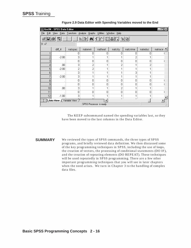
Figure 2.9 Data Editor with Spending Variables moved to the End
The KEEP subcommand named the spending variables last, so theyhave been moved to the last columns in the Data Editor.
We reviewed the types of SPSS commands, the three types of SPSSprograms, and briefly reviewed data definition. We then discussed someof the key programming techniques in SPSS, including the use of loops,the creation of vectors, the processing of conditional statements (DO IF),and the creation of repeating elements (DO REPEAT). These techniqueswill be used repeatedly in SPSS programming. There are a few otherimportant programming techniques that you will see in later chapterswhen the need arises. We turn in Chapter 3 to the handling of complexdata files.
SUMMARY

Complex File Types 3 - 1
SPSS Training
Complex File Types
IntroductionASCII Data and RecordsFile TypesSyntax BasicsData File StructureReading a Mixed FileErrors in the DataGrouped File Type Without Record Information
Most SPSS users find that the standard DATA LIST command issufficient to read the great majority of the data files theynormally encounter. This is because most data files are
rectangular, i.e., they contain the same number of records per case, thedefinition of a case is consistent throughout the file, and the variables tobe defined are identical for each case. There are, however, situations inwhich the above conditions do not hold. One example is a file at a medicalcenter with two types of records, one for inpatients and one foroutpatients, with identical variables located in different column positionson each type of record, and some variables unique to each type of patient.A standard DATA LIST cannot correctly read such a file and create aseparate case for each patient type.
To handle such a data file and any other that is non-rectangular,SPSS supplies two general solutions. The first is to use a FILE TYPEcommand, which allows the use of predefined file types that readgrouped, mixed, or nested files. The second solution is to allow the user totake complete control of the process of reading data with an INPUTPROGRAM command. This chapter discusses the use of file types; thenext chapter covers input programs. A third solution is to read the filewith a standard DATA LIST command, then use other programmingtechniques to restructure the file, such as VECTOR and LOOP. We willalso illustrate this approach in subsequent chapters.
Before reviewing the various file types, we need to discuss somebackground information.
Chapter 3
Topics
INTRODUCTION

SPSS Training
Complex File Types 3 - 2
SPSS assumes that complex files are in ASCII format so that they can beread with a DATA LIST command (within the complex file types). Filesthat are stored in a spreadsheet or database format cannot be readdirectly by SPSS with these techniques. In that case, you have twooptions. You can write out an ASCII file from the other software and thenread it into SPSS with a complex file definition. Or you can read the fileinto SPSS as you normally would, temporarily creating a working filewith an incorrect format for analysis. You can then use variousprogramming techniques to restructure the file.
The use of complex file types requires an understanding of a record.For SPSS, a record refers to a physical line of data in an ASCII data file.Technically speaking, a record ends with a carriage return and a line feed(these are invisible to users in most software). In practice, if you open adata file in a text editor, such as Notepad, each line will correspond to arecord in the data file. However, this is not always the case in wordprocessing software that wraps lengthy lines, so be careful when dealingwith a file for which you do not have a codebook that lists record length.
It is common to have several records for each case you plan to createin the final SPSS data file or to have several cases on one physical record.Understanding what constitutes a record and what the case definitionshould be in the final SPSS file is part of the art of successful data inputprogramming.
In general, ASCII text data files can be in either fixed or delimitedformat. Because complex file types must be able to locate case and/orrecord variables, though, complex data should be stored in a fixed-formatASCII text file.
The three available file types within the FILE TYPE command are:
Grouped: This is a file in which all records for a single caseare located physically together. Each case usually has onerecord of each type. Each record should have a caseidentification variable. This type of file is often identical to astandard rectangular file, the difference being that a groupedfile type allows additional checking for errors because ofmissing and out-of-sequence records, since SPSS normallyassumes that the records are in the same sequence withineach case.
Mixed: This is a file in which each record type defines a case.Some information may be the same for all record types butcan be recorded in different locations. Other information maybe recorded only for specific record types. Not all record typesneed be defined, so this is often a very efficient method toread only part of a data file.
ASCII DATA ANDRECORDS
FILE TYPES

Complex File Types 3 - 3
SPSS Training
Nested: This is a file in which the record types are related toeach other hierarchically. An example is a file containingschool records and student records, where all the studentsattending one school have their records placed together afterthe school record. Usually the lowest level of the hierarchy,the student in this example, defines a case. Information fromthe higher-level records, perhaps overall GPA at the school, isusually spread to the lower-level record when the case isdefined. All record types that form a complete set should bephysically grouped together, with an optional case identifieron each record. It is worth noting that record types can beskipped when reading the data, resulting in the creation ofcases at a higher level in the hierarchy.
Complex file type programs are begun by the command FILE TYPE andclosed with the command END FILE TYPE. These two commands encloseall definitional statements. One of the three keywords GROUPED,MIXED, or NESTED must be placed on the FILE TYPE command. Thecommands that define the data must include at least one RECORD TYPEand one DATA LIST command, though it is common to have several. Oneset of RECORD TYPE and DATA LIST commands is used to define eachtype of record in any data file. The definition of a case, again, dependsupon which FILE TYPE is specified.
The RECORD subcommand is required and names the columnlocation of the record identification information and, optionally, thevariable that will store this information. A CASE subcommand is alsoavailable (and required for a grouped file) that specifies the name andlocation of the case identification information.
This syntax illustrates the basic structure,
FILE TYPE (Grouped, Mixed, or Nested) FILE = 'Your File' /RECORD = RECID 4 CASE = ID 1-3.
RECORD TYPE 1.DATA LIST / your variables and column locations here.RECORD TYPE 2.DATA LIST / more variables here.etc.END FILE TYPE.
All three file types have subcommands available that warn the userwhen records and cases are encountered that don't meet the definitions ofthe file type, record, and case. This warning can include situations whenrecords are missing.
After the FILE TYPE--END FILE TYPE structure is processed, arectangular active file is created, no matter the original structure of theraw data file.
SYNTAX BASICS

SPSS Training
Complex File Types 3 - 4
To further illustrate the three types of files, we display samples of datafiles that can be read as grouped, mixed, or nested files.
A grouped data file often looks identical or very similar to a standardrectangular data file. However, a grouped file often has one or more of thefollowing problems:
1. A different number of records for each case2. Records out of order3. Records with the wrong record number4. Duplicate records
These situations all mean that SPSS will not read the filesuccessfully with a simple DATA LIST command. The structure of asimple grouped data file is shown in Figure 3.1.
Figure 3.1 Grouped Data File for Hospital Patients
DATA FILESTRUCTURE
GROUPED DATA
These data are from a hospital and contain information on tests andprocedures administered to each patient. Each patient’s data begins witha record that lists identifying information. The second and subsequentrecords include information on a test that was given, the date of the test,and the cost. Each record after the first defines a test, but we would likethe case definition to be a patient. The problem is that a different numberof tests is given to each patient, so we cannot specify the same number ofrecords for each patient.
A CASE subcommand is required on the FILE TYPE command inaddition to the RECORD subcommand. Records with a missing orincorrect case identification information cannot be corrected and placedwith the correct case, but SPSS will warn you about the problem.
All defined variable names for a grouped file must be unique becausemultiple records will be put together to form one case. By default all

Complex File Types 3 - 5
SPSS Training
instances of missing, duplicate, out of range (called "wild") or out-of-orderrecords will result in warnings from SPSS.
A mixed raw data file looks quite different than a rectangular data file.Again, a MIXED file type is used when each record type defines aseparate case (though not all record types need be defined). Figure 3.2depicts a portion of the file MIXED.DAT that contains job information onemployees from a large company.
Figure 3.2 Mixed Data File For Employees
MIXED DATA
Columns 2-4 contain an identification number for each employee.This is necessary for the company but not important for a FILE TYPEMIXED definition. Column 6 contains the required record identificationinformation, in this case either a 1 or 2 (there is also a record number 3not shown). The company had three separate record-keeping systems foremployee information for each division. The data from all three haverecently been placed in one file for reporting purposes.
A standard DATA LIST cannot be used to read this file because someof the same information is in a different location for each record type.Salary is recorded in a different location for each record type, and othervariables are not recorded in each system. We will attempt to read thisfile in the first example.

SPSS Training
Complex File Types 3 - 6
A nested data file also looks quite different than a rectangular data file.A FILE TYPE NESTED command is used when the records in a file arehierarchically related. One example is a file with two types of records,one for each department in a company, and one for each of the employeesin that department. All the employee records for one department areplaced consecutively together, after the record for the department inwhich they are located and before the next department record.
The variable names on all the records must be unique because onerecord of each type will be grouped together to form a case. Since not allrecord types need be mentioned on the RECORD TYPE command, it ispossible to define a case at a higher level in the hierarchy, e.g., adepartment rather than an employee. In fact, a case can be defined at anylevel in the hierarchy of record types. Figure 3.3 depicts a nested data filefor a school district.
Figure 3.3 Nested Data File for School District
NESTED DATA
The file contains data on the performance of high school studentsorganized by homeroom and school. It contains three types of records:
Record 1: The high school record contains identifyinginformation on the school plus the school's overall GPA, SATverbal and SAT math scores.
Record 2: The homeroom record contains identifyinginformation on the homeroom plus the average GPA for allstudents in the homeroom.

Complex File Types 3 - 7
SPSS Training
Record 3: The student record contains identifying informationincluding the student's sex and academic track, plus GPA,SAT verbal and SAT math scores.
There is only one variable in common for all three records, the recordidentifying information in the first column.
The data file has no case identifying information, which is typical ofreal-life situations. That isn't a problem since SPSS simply stores thehigher-level record information, spreading it to each record 3 when itcreates a case for each student, retaining this information until anotherrecord type 1 is encountered. SPSS can still successfully create the caseseven when intermediate-level records are missing (a homeroom record, inthis instance).
We will read the employee mixed data file from Figure 3.2 (namedMIXED.DAT) into SPSS and create a rectangular file with a case for eachemployee.
Here is a codebook table for the three types of employee recordsystems.
RECORD 1 RECORD 2 RECORD 3VARIABLE LOCATION LOCATION LOCATION
ID 2-4 2-4 2-4RECORD ID 6 6 6AGE 8-9 8-9 8-9SEX 11 11 11SALARY 13-17 22-26 13-17TENURE 19-20 19-20 19-20JOBCODE 22 17 not recordedLOCATION 24 15 22JOBRATE 26 13 not recorded
Not only are variables like SALARY recorded in different locations,but two variables, JOBCODE and JOBRATE, were not recorded on record3, which was the oldest record-keeping system. When the same variable,e.g., AGE, is defined by more than one record type, the format type andlength should be the same on all records. SPSS uses the first appearanceof the variable for the active file dictionary.
The appropriate commands to read this file are included in Figure 3.4and are in the file MIXED.SPS.
Click on File..Open..SyntaxIf necessary, switch directories to c:\Train\ProgSynMacDouble-click on MIXED
READING AMIXED FILE

SPSS Training
Complex File Types 3 - 8
Figure 3.4 Mixed File Type Program
The command FILE TYPE begins the file definition and puts SPSSinto an input program state. The MIXED subcommand tells SPSS thatthis is a mixed data file. The data file is named here, not on the DATALIST commands that follow. The only other required subcommand isRECORD to specify the record identification variable. The equal sign isnot required following RECORD or FILE. The record variable is incolumn 6 and will be named SYSTEM. For the employee data it isimportant to retain information that tells us under what record systemthe data were created because of duplicate IDs under each system; often,though, the record variable doesn’t need to be retained in the final file. Inthat case, it can be declared a scratch variable by beginning its namewith “#”.
Each employee data system, corresponding to a type of record in thedata file, gets its own RECORD TYPE command. The value specified onthe command (1, 2, or 3) refers to an actual value in the file MIXED.DATin the record identification position, here column 6 (refer to Figure 3.2).The DATA LIST command following each RECORD TYPE commanddefines the variables for that record type. Notice how SALARY is incolumns 13-17 for record types 1 and 3 but in columns 22-26 for recordtype 2.
An optional subcommand on the FILE TYPE command is WILD,which tells SPSS to issue a warning when it encounters undefined recordtypes in the data file. The default is NOWARN, so SPSS simply skips allrecord types not mentioned and does not display warning messages.

Complex File Types 3 - 9
SPSS Training
The input program state ends with the END FILE TYPE command,which is followed by labeling commands and then a Frequenciescommand. FILE TYPE--END FILE TYPE are not procedures and do notcause the raw data file to be read, so they must be followed by either anEXECUTE command or another procedure.
To run all the syntax
Click Run..All
SPSS displays the commands in the Viewer window (not shown) andthen the frequency table for SYSTEM. We can see that there are 212employees in the file, created from 212 records, and that there are 52 ofrecord type 1, 122 of record type 2, and 38 of record type 3 in the data file.All the information on, for example, salary, has now been placed in onecolumn despite its two different locations in the data (if you wish, switchto the Data Editor to verify this).
Figure 3.5 Frequency Table for System

SPSS Training
Complex File Types 3 - 10
We will illustrate what occurs with undefined record types by once againreading the file MIXED.DAT. Because warning messages are turned offby default, we were unaware that there are in fact 213 records, oremployees, in the file. However, the 213th case has an error in its recordtype, as shown in Figure 3.6.
Its record type should be a “3” but is instead a “4.”
Figure 3.6 Error in MIXED.DAT
ERRORS IN THEDATA
SPSS skipped this employee’s record because it was not defined on aRECORD TYPE command, but didn’t warn us. Let’s tell SPSS to do that,then reread the file.
Click Window..MIXED - SPSS Syntax Editor to return to thesyntax file
Add the subcommand /WILD=WARN to the end of the FILETYPE command, but before the period (.)
Figure 3.7 Modified File Type Command to Add Warnings From SPSS

Complex File Types 3 - 11
SPSS Training
After you have carefully added this subcommand, rerun all thecommands by
Clicking Run..All
When SPSS switches to the Viewer, you will now see a warningmessage and a note in the log under the FREQUENCIES command, asshown in Figure 3.8. The warning message is clear, telling us that therecord type (4) was ignored when building the file. You can verify this bylooking at the frequencies output, which lists only 212 cases.
The exact position of the problem is noted in the message that beginswith “Command line:”. The critical information is that it was on case 213that SPSS encountered an unknown record ID, whose value is 4. SPSSalso conveniently lists the actual line of data from the file MIXED.DATfor reference. Obviously, warnings can be helpful in finding and fixingerrors in data entry or definition.
Figure 3.8 Warning Messages for Undefined Record Type 4
It is now possible to use the file created via the FILE TYPE MIXEDcommand to report on either the total group of employees, or differencesbetween employees across record-keeping systems.

SPSS Training
Complex File Types 3 - 12
If you plan to read a file with known errors, you might think that youwant to be warned every time there is a problem defining an SPSS datafile. However, this is not always the case. If it is a large data file withmany errors, SPSS could possibly generate hundreds, even thousands, ofwarning messages. It is unlikely that you will care to scroll through allthat output. In recognition of this, the maximum number of warningsSPSS will display has been set relatively low, to a value of 10. When youdo want to see more warnings, use the SET command with this syntax:
SET MXWARNS = 100. (or to whatever value is appropriate)
Reading either a grouped or nested file into SPSS isn’t much differentthan reading a mixed file in terms of the syntax. However, one situationthat causes problems yet is still relatively common, and therefore worthexploring, is when you wish to use FILE TYPE GROUPED but don’t havea record identification variable. This is fairly common, especially becauseany rectangular data file can be read with either a standard DATA LISTor via a FILE TYPE GROUPED format. The advantage of the latter isthat SPSS will fix any problems with out-of-order records and read thefile correctly if there are missing records. However, a record type variableis needed in each instance, and you may not have created one for whatyou knew was a standard rectangular file format.
Our example here is a little more complicated. Figure 3.9 displays asmall data file that stores information on students in a statistics classand their scores on each of three assignments. There is an identificationvariable for the student in column 2, but no numeric record identifier totell SPSS that the first record has information on the first quiz, thesecond record on the first homework assignment, and the third record onthe first test. Moreover, student 2 did not complete the first homeworkassignment and so only has two records, which is the real problem.
If this file had been created with one record for each student, andeach assignment in a separate column, it would be a straightforward taskto read it into SPSS.
Figure 3.9 Grouped Data File
Analysis Tip
GROUPED FILETYPE WITHOUT
RECORDINFORMATION
We should point out that the score type (quiz1, etc.) field can be used as arecord type identifier, although it is a string field. However, we willignore this in order to demonstrate another method of reading the file.
Note

Complex File Types 3 - 13
SPSS Training
What we want to do is read this data file and create three cases, onefor each student. We also want to create three variables, one for each typeof assignment, and just as important, we want SPSS to realize that thesecond student’s second record has his score for the test, not thehomework, assignment.
There are two methods to approach this problem without using amore complex INPUT PROGRAM command sequence.
1) Read the data into SPSS, create a record identifier, write thedata back out as an ASCII file, then read it back in usingFILE TYPE GROUPED.
2) Read the data into SPSS, create a record identifier, thenmanipulate the data to create the necessary variables.
The latter choice is clearly preferable because it requires fewer passesof the data file. The file GROUPED.SPS contains the commands toimplement the second method.
Click on File..Open..Syntax (move to c:\Train\ProgSynMacfolder)
Double-click on GROUPED
Figure 3.10 Program to Read a Grouped File
The DATA LIST command reads GROUPED.DAT as if it were arectangular file. The interesting techniques in this program are whathappens after the file is read.

SPSS Training
Complex File Types 3 - 14
First, we create a RECORD variable with the LAG function. Initially,RECORD is set to 1 for each case. Then, when the current case has thesame ID as the previous case, RECORD is set equal to the value ofRECORD for the previous case plus one. When the previous case was adifferent student, then this statement is not executed and RECORDremains at 1, i.e., it is reset to 1 for each student’s first record. Thiscreates the desired record identification variable. To see this
Highlight the lines from DATA LIST to the first LISTcommand
Click on the Run button
Figure 3.11 List Output Showing Record ID
When creating programs that read or transform data, it is very helpful indebugging your programs to list out the data after an action or series ofactions is executed. If you don’t do this, then it will be very difficult tofigure out where things went wrong. Following this advice, the LISTcommand has been placed at four spots in the program. It is better to erron the side of excess here.
Our problems are not yet solved, though. Student 2 didn’t completethe homework, but the value of RECORD for his test1 score is 2, not 3.The set of IF statements fix this problem. They assign the correct value ofRECORD for each type of assignment, so that student 2’s test1 score willnow be listed as record type 3.
Switch to the GROUPED - SPSS Syntax Editor windowHighlight the lines from IF to the next LIST command
Click on the Run button
In the Viewer (not shown) we can now see that the value of RECORDfor the second line (or case) for student 2 has been changed to a 3.
Analysis Tip

Complex File Types 3 - 15
SPSS Training
One task remains, and that is to take these 8 cases in the Data Editorand turn them into 3 cases. As mentioned above, we could write this fileout and then read it back into SPSS, but that is cumbersome. A bettermethod is to use the AGGREGATE command. For analysis purposes, it isbest to create a separate variable or column for each assignment. If wesimply aggregate the current working file by student ID, that won’thappen. Why?
To create these new variables (three in this instance), we can takeadvantage of the VECTOR command we saw in Chapter 2. The VECTORcommand creates a new vector, SCORE_, with three elements. TheCOMPUTE statement then assigns the value of SCORE for a case to anelement of SCORE_ based on the value of RECORD. In other words, forthe first record type (quiz1), SCORE_1 gets the value of SCORE for thatcase, the quiz1 score. The values of SCORE_2 and SCORE_3 for that caseare system-missing. For the second record type (for hmwk1) SCORE_2gets the value of SCORE for that case, and SCORE_1 and SCORE_3 aresystem-missing.
It’s probably easier to see this in action.
Switch to the GROUPED - SPSS Syntax Editor windowHighlight the lines from VECTOR to the next LIST command
Click on the Run button
Figure 3.12 List Output Showing Vector SCORE_
The values for each assignment or test have been placed in separatevariables, with the quiz1 score in SCORE_1, the hmwk1 score inSCORE_2, and the test1 score in SCORE_3. However, there are stillthree cases for each student, with lots of missing data, and all we need isone case for each student to calculate appropriate statistics.

SPSS Training
Complex File Types 3 - 16
A file with that structure can be created using the AGGREGATEcommand, which changes the case base in a file and calculates summarystatistics for the new case base. For example, in a file of customers thatbuy five different products, AGGREGATE can create an SPSS data filewhere the case base is product (and so there are only five cases), withinformation such as the number of customers who bought each product,the mean age of customers who bought that product, and so forth.
There are three necessary subcommands for AGGREGATE, as shownin Figure 3.10. The OUTFILE subcommand tells SPSS whether to savethe new data file to disk or to make it the current working file in the DataEditor. The asterisk means to replace the current working file with thenew one. The BREAK subcommand defines the case base for the new file.By breaking on the variable ID, which here has only three unique values,we will create a file with three cases. The aggregated variablessubcommand creates the summary variables in the new file. Its format is
LIST OF NEW VARIABLES = FUNCTION (LIST OFEXISTING VARIABLES)
where you define new variable names on the left of the expression, anaggregate function on the right, followed by the same number of existingvariables that will be used to create the new variables. In our example,we use the MAX (maximum) function to create three variables calledQUIZ1, HMWK1, and TEST1, based on the maximum value of SCORE_1to SCORE_3 for each ID value. Why does this accomplish our task? Couldwe have used a different function?
To finish the program
Highlight the AGGREGATE and LIST commands
Click on the Run button
Figure 3.13 List Output Showing New Assignment Variables
The output from LIST demonstrates that there are only three cases inthe new file, one for each student. Three new variables have been created,one for each assignment. This makes it easy to calculate statistics foreach assignment. And student 2 has been correctly assigned a missingscore for HMWK1. Since AGGREGATE only creates the new summary

Complex File Types 3 - 17
SPSS Training
variables we define, the variables ASSIGN, SCORE, RECORD, andSCORE_1 to SCORE_3 are gone, which is fine. You may also want to lookat the Data Editor (not shown) to see the file format.
Unlike the definition of complex file types, every command in thisprogram could have been created from the dialog boxes except VECTOR.As this course is generally concerned with SPSS programming, weinstead worked from a Syntax file. Either approach is acceptable,although seeing the syntax often helps your understanding, and itcertainly lets you apply the same type of program in the future to anotherdata file.
We reviewed the types of complex files, their structure, and the SPSSsyntax used to read these data files. We illustrated the use of complex filetypes by reading a mixed data file, then discussed how data errors arehandled by SPSS. We then showed how to read a grouped file with an oddstructure and no numeric record type information.
Analysis Tip
SUMMARY

SPSS Training
Complex File Types 3 - 18

Input Programs 4 - 1
SPSS Training
Input Programs
IntroductionSyntax BasicsChanging the Case Base of a FileEnd of Case ProcessingEnd of File ProcessingChecking Input ProgramsIncomplete Input ProgramsReading Files with Missing IdentifiersWhen Things Go Wrong
There are situations where you encounter non-rectangular rawdata files that cannot be read directly with the complex file typesprovided by SPSS. For those situations, SPSS offers an input
program facility, as mentioned in Chapter 2, that has the capability toread essentially any type of ASCII data file. The ability to read a file willat times depend upon the cleverness of the user, as really odd files mayrequire creative solutions.
An input program can also be used to create data that match a targetdistribution, often for purposes of teaching or illustration. In other words,an input program can create data from nothing (this is the one time thatSPSS provides a free lunch, so to speak).
For very large files, input programs also offer great efficiencies, evenif the file is a standard rectangular data file. An input program can beused to select only certain cases as the file is read, saving one pass of thedata. Or it can concatenate raw data files, saving on having to createSPSS data files of each. And input programs can perform the equivalentfunctions of a grouped, mixed, or nested file type, but with addedflexibility.
The user is in charge of case definition when writing an inputprogram, so careful attention must often be paid to where in the programstream a case should be created. At times, you may also need to tell SPSSwhen to stop reading the data and create a working data file.
Chapter 4
Topics
INTRODUCTION

Input Programs 4 - 2
SPSS Training
The commands INPUT PROGRAM and END INPUT PROGRAM enclosedata definition and transformation commands that build cases from inputdata. At least one file definition command, such as a DATA LIST, mustbe included in the structure. Essentially any transformation commandscan be placed within an input program structure, but no procedures. Thismeans that you can use COMPUTE, IF, DO IF, REPEATING DATA,LOOP, or any of the other transformation commands that may help tocreate a working data file.
It is very important to understand that SPSS processes the inputprogram commands on a case-by-case basis. This may be hard to graspintuitively, given that an input program creates the definition of a case asit is executed, but we will illustrate this concept below to provide aconcrete example. Without comprehending this point, input programsmay remain somewhat mysterious in their operation.
We begin our exploration of input programs with an example thatincludes vectors and looping. Figure 4.1 displays a small data file. Thisdata file is to be used in an experiment on the effect of a drug onhypertension. Each person’s data consist of 15 measurements, recorded inthree sets of five numbers. Five different characteristics of each personwere recorded at three time points (hence the three records). Thus for thefirst person, the first five numbers are 1, 2, 3, 4, and 5, for the fivemeasurements at time 1. In this small test file, there are six lines of datafor two persons.
Figure 4.1 Data File with Three Records Per Case
SYNTAXCOMPONENTS
EXAMPLE 1:CHANGING THE
CASE BASE OF AFILE
However—and this is the problem with the file structure—we wish toflip the data because measurements of each characteristic came in sets ofthree that logically should be grouped together. Thus, the threemeasurements for the first characteristic of the first person are not 1, 2,and 3, but 1, 9, and 0. That is, they are the first numbers in each record.The three measurements for the second characteristic are 2, 8, and 0, andso forth for the remaining three characteristics.

Input Programs 4 - 3
SPSS Training
When we are done, the SPSS data file should look like Figure 4.2. Inthe restructured file, the rows have become columns and the columnshave become rows, separately for each person. That is our goal. It isusually very important when using an input program to literally sketchout the equivalent of Figure 4.2 to have a clear goal in mind.
Note that typically such files would contain subject and characteristicidentifiers, and additional information. We drop these variables to betterfocus on the data reorganization. However, without such identifiers youcannot tell what is what within the file.
Figure 4.2 The Goal: A Restructured Data File
To open the program that carries out this task
Click on File..Open..SyntaxIf necessary, switch directories to c:\Train\ProgSynMacDouble-click on INPUT1

Input Programs 4 - 4
SPSS Training
Figure 4.3 Input Program to Invert a File
The key points of the program are these:
1) Read the file as it currently exists to create fifteen variables foreach person;
2) Use a vector and looping to read the first, sixth, and eleventhvariable for each person;
3) Put these three bits of information into three variables in anew case;
4) Do this four more times for each person, to create five cases forthe five characteristics being measured of each person.
The case basis can be changed as the file is read because we are stillin an input program structure. We will walk through each command ofthis program to show how it operates.
INPUT PROGRAM: This command begins the input programdefinition. No other specification is necessary or can be added.
DATA LIST: The command reads the file INPUT1.DAT. This is astandard DATA LIST command, but because there are threerecords per person, a RECORDS subcommand is used tospecify this to SPSS. Fifteen new variables are created, onefor each measurement. They are declared scratch variables sothat they are not retained on the new file that SPSS willconstruct. The syntax for the DATA LIST uses a “/” to indicatethat SPSS should read the next record in INPUT1.DAT.
VECTOR: This command creates a vector from the fifteenvariables.

Input Programs 4 - 5
SPSS Training
LOOP: We loop from 1 to 5 (using the scratch variable #I) becausewe want to create five new cases for each person.
COMPUTES: Each pass through the loop creates three newvariables, A, B, and C. For the first value of #I, which is 1, Ais equal to the value of #V1. B is equal to #V6, and C is equalto #V11. It is important that you understand why thishappens and that this operation puts the values of 1, 9, and 0in these three variables.
At this point, SPSS has 19 variables created, #V1 to #V15, #I,and A, B, and C.
END CASE: This command tells SPSS to create a case at thispoint and pass it on to the commands immediately followingthe input program structure, when the data have all beenread. When the case is created, all 16 scratch variables areignored, so SPSS creates a case with only A, B, and C, asdesired.
When SPSS first encounters the END LOOP command, it resets thevalue of #I to 2 and passes through the three COMPUTE statements andthe END CASE command again with that value. Recall from Chapter 3that looping occurs within a case in SPSS, not across cases. Since theinitial DATA LIST statement essentially created a (temporary) case fromeach set of three records, the five passes through the loop create five newcases from these three records, or five cases per person.
When looping is done for the first person, SPSS goes on to read thenext set of three records and do the same for this person, and this willcontinue until the end of the data file is encountered.
END INPUT PROGRAM: When the physical end of the fileINPUT1.DAT is encountered, SPSS then writes out a finalversion of a working data file to the Data Editor, with onlythe variables A, B, and C. However, an input program is atransformation and so is not executed until SPSS encountersa procedure or the EXECUTE command. Here, we forceexecution with the LIST command (an SPSS procedure).
Let’s run the complete program.
Highlight all the lines in the program.
Click the Run Button
The commands are echoed in the Viewer, and the output from LISTshows that the file has been inverted as desired. The variables A, B, andC for the first case have values of 1, 9, and 0.

Input Programs 4 - 6
SPSS Training
Figure 4.4 List Output Showing New File Structure
Given the file restructuring capabilities of SPSS, we certainly couldhave read the data file without an input program, then changed the casebase with such commands as AGGREGATE afterwards. But an inputprogram is more efficient than such techniques, especially as a file growslarger. When you have the choice between these two approaches, an inputprogram is usually the better choice.

Input Programs 4 - 7
SPSS Training
END OF CASEPROCESSING
A basic problem that many people have when writing input programs ishow to properly handle end of case and end of file processing. We can usethe program INPUT1.SPS to illustrate the complexities of thesedecisions.
In Figure 4.5, the program has been slightly modified by switchingthe order of the END CASE and END LOOP statements.
Figure 4.5 Program With End Loop Before End Case
What type of data file will this structure create? How many cases willbe created? Why?
The answer is shown in Figure 4.6.

Input Programs 4 - 8
SPSS Training
Figure 4.6 New SPSS Data File
What happens is that the new program still tells SPSS to loop fivetimes within a case, but the second loop replaces the values of A, B, and Cwith new values, the third does the same, and so forth. After the fifth andlast loop, the values of A, B, and C for the first case are 5, 5, and 0—thevalues for the last number in each of the three records. At this point, wethen tell SPSS to create a case. Since we effectively didn’t change thecase basis from what the DATA LIST command created, we end up withonly two cases, one for each person. This is not what we intended, and itillustrates the importance of correctly placing the END CASE command.
Fortunately, it’s relatively easy to experiment in this fashion andusually straightforward to see the effect of command placement.

Input Programs 4 - 9
SPSS Training
When you write an input program, you can control all aspects of case andfile creation. Often, though, file creation is determined by SPSSautomatically when it runs out of raw data after reading to the end of anASCII data file. At that point, it creates the working data file. However,you can control this decision, and we illustrate this capability bymodifying INPUT1.SPS slightly.
Click Window...INPUT1 - SPSS Syntax EditorAdd a blank line after END LOOPType the command END FILE. in this lineMake sure END CASE precedes END LOOP
The syntax editor should appear as Figure 4.7
Figure 4.7 Modified Program with End File Command Added
END OF FILEPROCESSING
At first glance, it might appear that this END FILE command isredundant. After all, it occurs after both the END CASE and END LOOPcommands. What effect might this command have? Run the program by
Highlighting all the lines
Clicking on the Run Button
The output from LIST says that SPSS created five cases, not ten.Inspection of the output shows that only data from the first person in thefile was used to create the working data file. The program operatedcorrectly for the first person, creating five rows with three variables, butit dropped the second person (and it would have dropped any subsequentrecords).

Input Programs 4 - 10
SPSS Training
The END FILE command was encountered before END INPUTPROGRAM. This means that SPSS passed the decision of when to finishreading the data file to the user. Our program operates as follows:
1) Read the first three records;2) Loop five times for the first person and create five cases with
three variables each;3) Don’t read the next set of three records. Instead, stop reading
the data file and write out a working file.
Figure 4.8 List Output Showing Data From Only One Person
Like END CASE, END FILE takes effect immediately, which is whyit produces this result. It also has this effect because SPSS processes filesby case. Logically, it is true that the end of file comes just after the end ofthe looping, but in SPSS programming the entire input program is readand processed for each case before the next case is read and defined.Thus, the END FILE command is encountered for the first case, andSPSS stops reading INPUT1.DAT.
In Chapter 3 we strongly advised you to place LIST commands liberallythroughout your programs when creating and debugging them.Nevertheless, an input program is a transformation, and so procedurescannot be placed within its structure.
This makes it imperative to work with small but representative fileswhen writing an input program, as we did in the first example. Thelarger the file, the more that can go wrong and the harder to figure outwhat went wrong.
CHECKING INPUTPROGRAMS

Input Programs 4 - 11
SPSS Training
There are two types of mistakes to make in writing input programs. Thefirst is a logical mistake, such as placing the END CASE command in thewrong location. The second, just as common, is to make a typing errorwhen creating commands. In either instance, strange things can happenthat are directly related to the fact that an error occurred in the middle ofan input program structure.
When SPSS is in the input program state, it hasn’t yet created aworking data file. Moreover, SPSS will be in the middle of variousdefinitions, which are not necessarily reset when the program fails. Inother words, when there is an error in an input program, SPSS will oftenremain in the input program state. This isn’t good, because when you fixan error and rerun your program, SPSS will become confused when itsees an INPUT PROGRAM command when it is already in that state.
To illustrate this problem, we will make the most common type ofsyntax error and see what it causes.
Click Window..INPUT1 - SPSS Syntax EditorRemove the line END FILE.Remove the period after the END CASE commandHighlight all the lines
Click on the Run button
If necessary, switch to the Viewer window
When this program is run, SPSS understandably complains, althoughit doesn’t actually state that the END CASE command is missing aperiod. Instead, it becomes confused about the text “END LOOP” which itthinks the user meant to add to the END CASE command (which has nosubcommands).
Figure 4.9 Errors Created in an Input Program
INCOMPLETEINPUT
PROGRAMS

Input Programs 4 - 12
SPSS Training
Notice that the second error, on END INPUT PROGRAM, explicitlystates that there is an error created while there is an unclosed complexfile structure. If you take a look at the Data Editor (not shown), you willsee that it is empty, although it does have the three variables A, B, and Ccreated.
Now let’s fix the error and run the program again.
Click Window...INPUT1 - SPSS Syntax EditorAdd a period after the END CASE commandHighlight all the lines
Click on the Run Button
If necessary, switch to the Viewer
In Figure 4.10, you can see what occurred. After processing the firstcommand, INPUT PROGRAM, SPSS complained with an error that sucha command is not allowed in the set of file definition commands, i.e.,those commands that normally follow an INPUT PROGRAM command.
Figure 4.10 Errors Created When Rerunning the Input Program
The remainder of the program is not correctly processed, so onceagain the Data Editor is empty of cases.
Fortunately, there is an easy solution to this problem, which SPSSmentioned in Error Message 101: Use the NEW FILE command. Thiscommand clears the working data file and removes any unclosed loops orfile structures from memory. Let’s add it to the program.

Input Programs 4 - 13
SPSS Training
Click Window...INPUT1 - SPSS Syntax EditorAdd the command NEW FILE. on its own line before INPUT
PROGRAM (Alternatively, click File..New..Data)
Your screen should appear similar to Figure 4.11.
Figure 4.11 New File Command Added
Highlight all the lines
Click on the Run Button
The program has now worked flawlessly with no errors. The outputfrom LIST shows the correct file structure of 10 cases. Figure 4.12provides a look at the file in the Data Editor. The NEW FILE command isso important that, until you become accomplished at writing inputprograms, and whenever you first start writing such a program, werecommend you include it as the first command and run it each timealong with the other commands.

Input Programs 4 - 14
SPSS Training
Figure 4.12 Data Editor With Five Cases Per Person
After beginning with a relatively uncomplicated example, we nextattempt to read a deceptively simple file. This example will illustrateseveral features of input programming, including the ability to rereadlines of data.
Occasionally you may encounter files which require special treatmentbecause they have no case and/or record identifiers on every record.Figure 4.13 is an example of such a data file, recording order informationfor a consumer products company. Each customer’s data begins with aheader record that contains information on billing ID, the location of thecustomer, and the general product type. In this small data file, acustomer can make up to three orders, represented by the recordsfollowing the header record. The order records contain the price and thetype of order, 1, 2, or 3.
EXAMPLE 2:READING FILES
WITH MISSINGIDENTIFIERS

Input Programs 4 - 15
SPSS Training
Figure 4.13 INPUT2.DAT File
In this file, there are multiple records per customer, and an unequalnumber per customer, since not every customer has made three orders.The goal is to create an SPSS data file with one case per customer. Inaddition, the three order types can come out of order—for the firstcustomer, the third order appears second—and we also want to recordthese correctly in sequence in the SPSS data file. As always, it isimportant to have a picture of the goal in mind, so Figure 4.14 displaysthe SPSS Data Editor with the target file structure. Each customer,identified by the billing number, represents one case, and the orders arenow in the correct sequence, so that order number 3 for the first customeris placed in the variable VALUE3, even though it appeared on the secondrecord.
Figure 4.14 Target SPSS File Structure

Input Programs 4 - 16
SPSS Training
Would it be possible to read this file with a FILE TYPE GROUPED?If not, what are we missing? What about FILE TYPE MIXED? Or FILETYPE NESTED?
The complications in the file are that the header record has no recordinformation, and the order records have no ID variable. We must takethis into account when reading the file.
Our task will be made much simpler by using the REREADcommand. To determine the type of record, it is necessary to read it. Thatsounds so obvious it’s not worth stating, but here is the difficulty: onceSPSS has read a record, it normally goes to the next record in the datafile. However, that’s no good here, because once we’ve read a record anddetermined whether it is a header or order record, we then want toreread it to store the necessary information in the SPSS data file.REREAD tells SPSS to do exactly that.
Let’s open the program that accomplishes the task of reading thisdata file.
Click on File..Open..SyntaxIf necessary, switch directories to c:\Train\ProgSynMacDouble-click on INPUT2
Figure 4.15 displays the program in the Syntax Editor window. Thegeneral method that will read this file is to:
1) Read a field from each record to test for record type.
2) If the record is a header record, build a case with the ENDCASE command from the information currently stored. Inother words, when a header record is encountered, we know anew customer’s records are being read, so we create a case forthe previous customer from the records just above this headerrecord. And if the record is the last record in the file, build acase and end the file with the END FILE command.
3) Read the header record with the appropriate DATA LIST.
4) If the record is not a header record, read the order type andcost as scratch variables so they are not retained in the finalfile.
5) Store the results into a vector created earlier in the program.

Input Programs 4 - 17
SPSS Training
Figure 4.15 INPUT2.SPS File
This logic is displayed graphically in Figure 4.16. As before, we willwork through the program one line at a time, explaining the logic behindeach command and the structure of the syntax.
Figure 4.16 Flow Chart For INPUT2.SPS

Input Programs 4 - 18
SPSS Training
The program begins with the INPUT PROGRAM command.
NUMERIC: This command initializes the variable REGION andthe three VALUE variables that will be used to create avector for the orders. These variables are initialized tosystem-missing, an important feature, because the value ofREGION will be used to determine when the first header isbeing read for the first case.
VECTOR: This command defines the vector ORDER from thethree VALUE variables.
DATA LIST: This is the first of three DATA LIST commands. Itdefines the file to be read, and it includes the ENDsubcommand, which defines the variable #LAST (a scratchvariable so it is not retained). #LAST is a logical variablewhich takes on only two values. It has a value of 0 exceptwhen the end of file is reached (after the last record), where itis set to 1. This will allow us to tell SPSS to create the lastcase and to end the file. We read only the variable #CHECKfrom each record, from column 3. That column has non-missing information only for header records. We could havechosen any column that differentiated a header record froman order record.
DO IF #LAST: This first DO IF checks for the value of #LAST.Since #LAST is a logical variable, the DO IF is executed whenthis condition is true, i.e., when #LAST is equal to 1. And thatoccurs when no records remain and the end of file is reached.
END CASE: Notice that this command is indented four spaces. Itis good programming practice to make programs morereadable by indenting lines that fall within a DO IF structure(or DO REPEAT or LOOP). SPSS commands can be indentedwithout the period in column 1 when running interactivelyfrom the Syntax Editor, but programs run in the productionfacility or with the INCLUDE command should include theperiod (or, alternatively, a plus sign or dash) to indent acommand.
The END CASE command, for the last record in the file, tellsSPSS to create a case. We must do this check because the lastrecord is not followed by another header record, which is thenormal method used to tell SPSS when to build a case.
END FILE: The command tells SPSS to create the working datafile, again because this is the last record.
COMPUTE: The COMPUTE command creates a logical variablethat allows us to check the record type, using the variable#CHECK from the first DATA LIST. When #CHECK issystem missing, #TESTREC is set to true, or 1. This occursfor order records. Why? When #CHECK is not system–missing, #TESTREC is set to false, or zero.

Input Programs 4 - 19
SPSS Training
DO IF #TESTREC=0: This second DO IF is the heart of theprogram. It checks to see whether #TESTREC is 0, whichmeans we are reading a header record, and so must create acase.
DO IF NOT(SYSMIS(REGION)): The third DO IF, nested in thesecond, creates a case when REGION is not system missing.This is true for every header record except the first, whereREGION was initialized to system missing by the NUMERICcommand. So for all header records except the first, this DOIF command creates a case.
REREAD: After creating a case, it’s time to get on with buildingthe next case, beginning with the header record we just read.Thus, the REREAD command tells SPSS to go back to thebeginning of this record.
DATA LIST: This second DATA LIST rereads the record with aformat appropriate for a header record.
ELSE IF #TESTREC=1: This block handles order records. Theheader test variable takes on values of 0 and 1. When it isequal to 1, that means that #CHECK is system missing, so weare reading an order record, which has no information incolumn 3.
REREAD: Once again, we must tell SPSS to reread the recordbecause SPSS had to read it once to see whether it was aheader or order record.
DATA LIST: The third DATA LIST command reads the twovariables that are on order records. It uses scratch variablesbecause this information will either be passed to otherpermanent variables or is unnecessary to retain.
COMPUTE: This command plugs the cost of each order into thecorrect element of the vector ORDER. For example, if#TYPE=2, then the second element of ORDER (VALUE2) isset to the value of #COST for that record.
END IF: This closes the last DO IF.
The program ends, as always, with an END INPUT PROGRAMcommand, then a LIST command to force program execution and checkour work.
To see this in operation:
Highlight all the lines in the program
Click on the Run button
When an input program works correctly, it all seems so deceptivelysimple. In Figure 4.17 we see the output from LIST. We have created

Input Programs 4 - 20
SPSS Training
SUMMARY
three cases as planned, retaining region, billing number, and producttype, and we have placed the costs in the correct VALUE variables. Thesecond customer has a missing value for VALUE2 because he made noorder of this type.
Figure 4.17 List Output With Three Cases
Creating a program such as INPUT2.SPS is not easy, though, withoutlots of experience at programming with SPSS or with other programminglanguages. Expect to make several errors when trying to create thisprogram, which, as noted previously, can be difficult to check becauseprocedures can’t be placed in the middle of the program to check yourwork. One important thing to do is to make sure you are working in anempty Viewer window, and to empty it out on a regular basis. Otherwise,as you execute the program, syntax errors from one run of the programwill blend with errors from subsequent runs, and it will be more difficultto recognize what needs to be fixed.
One error that is sometimes made is to ignore the need to tell SPSS tostop reading the data file. What makes the decision to use an END FILEcommand tricky is that, in general, there is no requirement within aninput program to tell SPSS when to stop reading the file. So in our firstexample, no END FILE command was necessary. This is becausenormally SPSS reads the last line of data, inputs it as instructed, sees anend–of–file marker in the raw data file, and writes out a working data fileautomatically.
In this program, however, we took control of the process with theEND subcommand on DATA LIST. We did this so we would be able tocreate the last case, but SPSS then passed end of file processing to theuser.
This chapter provided a brief look at input programs via the use of asimple example. We discussed the basics of writing such programs, andthe importance of controlling end of case and end of file processing. Wealso discussed how to check and correct input programs. We thenattempted a complex input program that read a data file with missingrecord and identification fields.
WHEN THINGSGO WRONG

Advanced Data Manipulation 5 - 1
SPSS Training
Advanced Data Manipulation
IntroductionSplitting a String Variable on a DelimiterReading Multiple Cases on the Same RecordAn Existing SPSS Data File with Repeating DataPrint Command for DiagnosticsPractical Example: Consolidating TransactionsAppendix: Identify Missing Values by Case
We have discussed how to read various non-rectangular filesin SPSS, using either input programs or complex file types. Inthis chapter, we consider some examples of how to further
manipulate data in SPSS, and we discuss a few additional commandsoften used in data transformation. The examples were chosen to bothillustrate potentially useful applications and to show the operation ofthese commands.
Chapter 5
Topics
INTRODUCTION

Advanced Data Manipulation 5 - 2
SPSS Training
Often users encounter ASCII data files that are comma delimited, ratherthan in fixed or freefield format. Comma delimited means that the valuesof variables are separated by commas. Many database software programscreate such files. An example of this type of file is displayed in Figure 5.1.
Figure 5.1 Comma–Delimited Data
SPLITTING ASTRING
VARIABLE ON ADELIMITER
SPSS does have an option to automatically read this type of file,under freefield input, but this example serves to illustrate methods usedwhen working with string fields. However, there should be ten values perrecord, but the first and second records have only 9 (because there areonly 8 commas). Standard freefield input will misread such a data file.(Note the LIST option on the DATA LIST command and the default TextWizard dialog choices (click File..Read Text Data) will read the datacorrectly.)
Also, on occasion a list of string values, separated by a delimitercharacter, are stored as a single field in a data file. For example, radiostations listened to, problems encountered with a product, products usedin the last month, etc.
Such files can be read without too much fuss. The method is based onthese steps:
1) Read all of each record as a long string variable;2) Search through this string for a comma, extracting the text
before this position as a variable;3) Replace the string with the contents following the comma, and
continue the process;4) Repeat until there are no more commas, which allows for
variable-length input fields.
To accomplish these tasks we need to utilize not only the VECTORand LOOP commands, but also the string transformation capability ofSPSS. The program that illustrates this procedure is namedCOMMA.SPS.
Click on File...Open..SyntaxIf necessary, switch directories to c:\Train\ProgSynMacDouble-click on COMMA

Advanced Data Manipulation 5 - 3
SPSS Training
Figure 5.2 Comma.sps Syntax File
We are going to read the small dataset from Figure 5.1, which isincluded as inline data in the program. This method will easily generalizeto any size file, and can be used to split an existing string variable intonew variables. We now discuss program execution, step by step.
DATA LIST: Each record of data is read in as one long stringvariable, 80 characters in width, with the name VAR. Doingso makes it possible to easily search through all the data andavoids the problem of missing data between commas. Thistrick—reading all the data as a long string—is a very commontechnique to read troublesome files.
VECTOR: The command creates a vector to store the actualvariables. 10 elements of SLOTS are created because thereare ten variables for each case. Each is given a format of A5(alpha field 5 columns wide) because a number of the fieldscontain string data.
COMPUTE: For each case, #I is initialized to 0, but note that thisis outside the loop that will be created next.
LOOP: This Loop command has no index value, so it mightappear as if it will not loop at all, or loop forever, but that isnot true. Looping will continue until the maximum number ofloops is reached (40), or until a condition is met on the ENDLOOP command.

Advanced Data Manipulation 5 - 4
SPSS Training
The two COMPUTE commands find the next comma and increment#I. The INDEX function in SPSS as used in the first COMPUTE has thisformat:
INDEX(variable,test string)
It returns an integer that indicates the starting position of the firstoccurrence of the test string in the variable. It returns 0 if the test stringis not found within the variable.
COMPUTE #COMMA: The INDEX function searches throughVAR for a comma. The syntax places the test string value inapostrophes (‘,’). It sets #COMMA equal to the position of thefirst comma it finds. Thus for the first case and the firstiteration through the loop, the value of #COMMA is 2.
COMPUTE #I: The value of #I is incremented by 1. The reasonwill become apparent in a moment.
We next encounter a DO IF–END IF structure. The two COMPUTEcommands within this structure are executed when #COMMA is greaterthan 0. When does this occur? Answer: when the value that the INDEXfunction returns is greater than 0, which occurs when a comma can befound in VAR. In other words, the COMPUTE commands are executedwhen there is a value to record from VAR.
The first COMPUTE uses the SUBSTR function. SUBSTR has thisformat:
SUBSTR(variable,position,length)
It returns the substring of the variable beginning at the positionindicated and running for the length specified.
COMPUTE: SLOTS(#I): Let’s see how this operates for the firstiteration of the loop. #COMMA is equal to 2, so this says totake a substring of VAR, beginning in column 1, for onecolumn. This means to read the first column of information (a“1”) and place it in the first element of SLOTS, because #I =1(now you can see why we increment #I once each loop). Sonow SLOTS1=1 and the first variable for the first case hasbeen created.
COMPUTE VAR: This command replaces the full 80-characterVAR with a shorter version, taking a substring beginning atcolumn 3, thus leaving out the “1” and the comma that followsit for the next iteration.
END LOOP: The looping only ends when #COMMA is equal tozero. This occurs when the INDEX function can’t find anymore commas, which means we don’t need to read any more ofVAR.

Advanced Data Manipulation 5 - 5
SPSS Training
If you’ve followed the program to this point, it might appear that ourdata file reading problem has been solved, but that’s not quite the case. Aline of data does not end with a comma, but this means that the last fieldwill not be stored by SPSS because the program as written requires acomma at the end of a field (so that the preceding characters can bestored in the vector SLOTS). The last field must be handled separately.
COMPUTE SLOTS(#I): This command takes the current value ofVAR and puts it in the element for SLOTS equal to thecurrent value of #I. Thus if the last bit of data is the tenthvariable, as for the third case, this command places 78 intoSLOTS10.
The LIST command then executes the preceding transformationstatements and checks our work. Before executing the program, let’s runthrough one more example. After the program places the value of “1” inSLOTS1, it does the following:
1) Computes VAR to be equal to“alpha,23453,,43553,,,sadfs,5435”
2) Loops again, since #COMMA is equal to 23) Computes #COMMA=64) Computes #I=25) Computes SLOTS2= substring of VAR from position 1 to 5 =
“alpha”6) Recomputes VAR, etc.
To see this in action:
Highlight all the lines from DATA LIST to the first LISTcommand
Click the Run tool button
Figure 5. 3 Ten New Variables Created
The output from LIST shows that the values from the raw data havebeen correctly placed in the appropriate variables, with missing data (ablank for string variables) inserted in the right spots. The tenth variablevalue is missing for both the first and second cases. To further illustratehow the program is functioning, switch to the Data Editor window.
Click on the Goto Data tool

Advanced Data Manipulation 5 - 6
SPSS Training
The variable VAR is retained in the file and has the value of 5435 forthe first case, 34 for the second case, and 78 for the third case. It storesthe last valid value in each record because that was the last field that didnot end with a comma.
Figure 5.4 Data Editor With New Variables and VAR
Note that the VAR column is narrowed in the Data Editor so both itand the SLOT variables are visible.
This file is now a regular SPSS data file and ready to be used foranalysis, but all the variables are strings. To make the variables that arenumbers into numeric variables, we use the NUMBER function. The DOREPEAT command simply affords an easy means to create a series ofeight COMPUTE statements. The NUMBER function requires twoarguments, the variable to be converted, and a format by which to readthe variable (here F5 for 5 characters, no decimal digits).
Click Window..COMMA - SPSS Syntax EditorHighlight the commands from DO REPEAT to LIST
Click on the Run tool button
After these commands are executed, the Viewer window displays alleight COMPUTE commands created from the DO REPEAT (not shown).Figure 5.5 displays a portion of the output from LIST with the numericversions of eight of the SLOTS variables. Why do these variables all havetwo decimal digits displayed?

Advanced Data Manipulation 5 - 7
SPSS Training
Figure 5.5 List Output with Numeric Variables
This program can be readily generalized by increasing the width ofthe long string variable VAR on the DATA LIST, by using more than oneof these variables if the record length is more than 256 characters (themaximum width for a long string variable), and by setting the number ofelements for SLOTS as high as necessary to create as many fields as existin the data. MXLOOPS may have to be set higher than the default of 40as well (use SET MXLOOPS= value.).
In Chapter 4 we discussed how to rearrange a file and change thecolumns into rows. At times you may be faced with the reverse situation:many cases stored in one record. This can occur whenever all informationfor one person or organization is stored in one record of data during dataentry for efficiency’s sake. You may later wish to place each occurrencewithin an ID into a separate case for analysis purposes (such as tocalculate aggregate statistics across cases). An example of such a file is inFigure 5.6.
READINGMULTIPLE
CASES ON THESAME RECORD

Advanced Data Manipulation 5 - 8
SPSS Training
Figure 5.6 A File With Multiple Cases Per Record
Each case has identifying information in the first two fields. It thenhas up to five fields of valid data, which could be customer orders,procedures in a hospital, exam scores, and so forth. This type of structurecan be thought of as repeating data, because each case contains repeatingbits of information that are of the same type.
SPSS supplies a predefined command that will read these types ofdata. The REPEATING DATA command must be used within an inputprogram structure, and it will build one new case for each repeatinggroup. All the repeating groups must contain the same type ofinformation, but there can be a different number of repeating groups foreach record.
The user must tell SPSS how many repeating groups of data are ineach record, but often files of this type do not include such information, asin Figure 5.6. This value can be created from the data, though, as wedemonstrate below. The sample program that reads these types of data isnamed Repeat1.sps.
Click on File..Open..Syntax (move to c:\Train\ProgSynMac)Double-click on Repeat1
The method of reading the file is not complicated.
1) Read the data with a standard DATA LIST command;2) Compute a variable that records the number of repeating data
groups;3) Use the REPEATING DATA command to create the cases.
You must supply the number of repeating data groups for theREPEATING DATA command, but there is no penalty in initiallyestimating too many of these on the DATA LIST. We illustrate this byhaving SPSS read up to six variables for the critical information eventhough no more than five appear on any input record.

Advanced Data Manipulation 5 - 9
SPSS Training
Figure 5.7 REPEAT1.SPS Syntax File
Specifically, the program does these tasks:
DATA LIST: Read in the variables ID and GROUP, which appearonce per record, and then read six variables for the repeatingdata.
COMPUTE: This command uses the NVALID function, whichreturns the number of nonmissing values in a set of variablesfor each case. This puts the number of occurrences ofrepeating data into the variable TOTNUM.
REPEATING DATA: The command has only three requiredsubcommands. The STARTS subcommand specifies thebeginning column of the repeating data segments, herecolumn 6. The OCCURS subcommand tells SPSS how manyrepeating data groups are on each record, and the DATAsubcommand tells SPSS the names, locations, and formats (ifnecessary) for each variable within the repeating groups.There can be many variables within each repeating group, butwe’ve kept things simple in this example and have only one.
END INPUT PROGRAM closes the input program structure, andit is followed by the inline data.
Run the program by:

Advanced Data Manipulation 5 - 10
SPSS Training
Highlighting all the lines
Clicking on the Run Button
Figure 5.8 List Output With All Variables
Twenty one cases have been created by SPSS, for the 21 separaterepeating data values in the input file. There are four repeating groupsfor the first record (117, 837, 947, and 594), so SPSS created four casesfrom the first input record. Although no input record had six repeatingdata groups, our specification of six input variables on the DATA LISTcommand didn’t cause any difficulty. SPSS simply created a sixthvariable, V6, that is missing for every case. The critical information, inaddition to ID and GROUP, is the information stored in VARVALUE,which came from the repeating data.
At this point, we could delete the variables V1 to V6 and TOTNUMfrom the file (though the latter might be useful for analysis), and save thefile as an SPSS data file. We then can compute such quantities as themean of VARVALUE for the whole file, which would have been verydifficult to calculate with the initial file structure.
A file in this format also allows us to study the data by customer byaggregating based on ID.
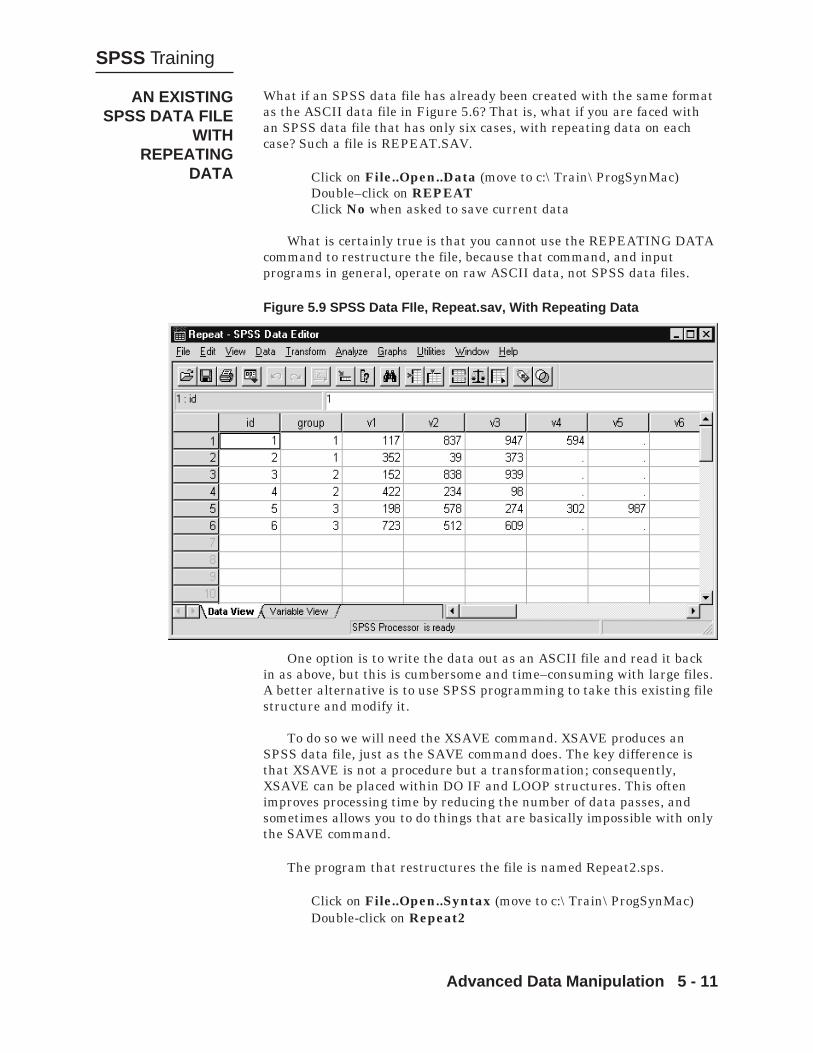
Advanced Data Manipulation 5 - 11
SPSS Training
What if an SPSS data file has already been created with the same formatas the ASCII data file in Figure 5.6? That is, what if you are faced withan SPSS data file that has only six cases, with repeating data on eachcase? Such a file is REPEAT.SAV.
Click on File..Open..Data (move to c:\Train\ProgSynMac)Double–click on REPEATClick No when asked to save current data
What is certainly true is that you cannot use the REPEATING DATAcommand to restructure the file, because that command, and inputprograms in general, operate on raw ASCII data, not SPSS data files.
Figure 5.9 SPSS Data FIle, Repeat.sav, With Repeating Data
AN EXISTINGSPSS DATA FILE
WITHREPEATING
DATA
One option is to write the data out as an ASCII file and read it backin as above, but this is cumbersome and time–consuming with large files.A better alternative is to use SPSS programming to take this existing filestructure and modify it.
To do so we will need the XSAVE command. XSAVE produces anSPSS data file, just as the SAVE command does. The key difference isthat XSAVE is not a procedure but a transformation; consequently,XSAVE can be placed within DO IF and LOOP structures. This oftenimproves processing time by reducing the number of data passes, andsometimes allows you to do things that are basically impossible with onlythe SAVE command.
The program that restructures the file is named Repeat2.sps.
Click on File..Open..Syntax (move to c:\Train\ProgSynMac)Double-click on Repeat2

Advanced Data Manipulation 5 - 12
SPSS Training
Figure 5.10 Repeat2.sps Syntax File
Not surprisingly, the program relies upon a vector and looping toaccomplish its job. It works in this fashion:
1) Create a vector to store the repeating data2) Loop as many times as there are repeating data groups3) Create the variable to store the repeating data group, and if it
is not missing, write a case to the file STACKDAT.SAV,retaining only the necessary variables.
Specifically, the commands do the following:
VECTOR: The new vector VREPEAT is created from the existingrepeating data variables, here V1 to V6.
LOOP: We loop as many times as there are repeating datagroups. However, requesting more loops than there aregroups will not cause an error or the program to functionimproperly.
COMPUTE VARVALUE: On the first loop, the value (117) of thefirst element of VREPEAT (V1) for the first record is placedinto VARVALUE.
DO IF: This is executed if the current element of VREPEAT is notmissing. In other words, the statements in the DO IFstructure are executed if there is a valid repeating data value.This check means that no cases will be created when there ismissing data, even when a record has fewer than 6 repeatingdata values.

Advanced Data Manipulation 5 - 13
SPSS Training
XSAVE: The XSAVE command has the same format as SAVE. Wename the output file and tell SPSS which variables to retain.Users often picture a SAVE command as being applied to thewhole file at once, but if that were true, XSAVE couldn’t writeout the data appropriately here. Instead, both SAVE andXSAVE write out one case at a time, until all the data fromthe current working SPSS file have been read. This meansthat XSAVE writes out the first case to STACKDAT.SAV,whose values are these:
ID GROUP VARPOSN VARVALUE
1 1 1.00 117.00
and waits for input from the next iteration of the loop.
In this manner, SPSS creates 21 cases from the original 6, one foreach valid repeating data group. The idea of looping through a record andwriting out the cases to an SPSS data file with XSAVE is the central ideaof this, and similar, SPSS programs.
The program closes with END IF and END LOOP. We then need toget the file STACKDAT.SAV to see the new structure.
Highlight all the lines from VECTOR to EXECUTE (do not runthe GET FILE command yet)
Click on the Run tool button
Switch to the Data Editor (click the Goto Data tool )
Figure 5.11 Data Editor Showing REPEAT.SAV With New Variables

Advanced Data Manipulation 5 - 14
SPSS Training
We are first looking at the existing file, not STACKDAT.DAV, so youcan understand better how this program functions. Two new variablesare created, VARPOSN and VARVALUE. The latter is system–missingfor every case because no input record had a sixth valid field of repeatingdata. What may be surprising is that VARPOSN is equal to 7, not 6, eventhough the LOOP command is designed to iterate six times. What SPSSdoes is execute the loop six times, then increment the value of VARPOSNto 7, and test for the loop ending condition (which is VARPOSN=6). Since7 is greater than 6, SPSS doesn’t execute another loop, but it has set thevalue of the index variable to one higher than the end of the loopsequence. This is how loops always operate.
Now let’s look at the new file structure.
Click Window..Repeat2 - SPSS Syntax EditorHighlight the two lines GET FILE and LIST
Click on the Run button
The output from LIST shows that we have created the desired filestructure. There are 21 cases in total, and we have only the variables weneed, unlike the program with the REPEATING DATA command, inwhich variables were dropped to create the final file.
Figure 5.12 List Output from STACKDAT.DAV
These examples have illustrated how there is often more than oneway to accomplish the same result in SPSS. If a file is small, it may makelittle difference which method is used, but for larger files, efficiency isoften important (see Chapter 8). This example also demonstrates how an

Advanced Data Manipulation 5 - 15
SPSS Training
existing file can be restructured, just as we did in Chapter 4 when wechanged columns into cases.
In the examples run thus far we frequently made use of the Listcommand to display values for specified variables in the active data file.One disadvantage of the List command is that it is a procedure. As aresult, List cannot be placed within a loop or Do If structure, and wouldbe of limited value in determining what is happening within suchstructures. Also, as a procedure the List command forces a data pass.Thus if we insert three List commands in a program, three data passesmust be performed, which is inefficient.
To answer these issues, SPSS has a transformation command calledPrint. It provides the same general features as List, but is atransformation. Print can be placed within Do If and loop structures, andcan provide detailed feedback about what occurs. However, be aware thatif a Print command is placed within a loop, then it will print a line ofoutput during each iteration of the loop for every case in the file. Suchoutput is extensive for large data files, so care must be taken. Below webriefly demonstrate the use of the Print command by inserting one intothe program run earlier that read a comma-delimited file.
Click Window..Comma - SPSS Syntax EditorInsert a blank line before the COMPUTE VAR=… lineType PRINT / '#Comma= ' #comma (F2) ' Var= ' var
(a50). (all on one line)
Figure 5.13 Comma.sps Program with Print Command Added
PRINTCOMMAND FOR
DIAGNOSTICS

Advanced Data Manipulation 5 - 16
SPSS Training
By default the Print command will print to the Viewer window, but itcan be directed to a file. Text can be added to a Print command byenclosing it in quote marks. We use this feature to identify the variableswhose values will be printed. Values for two variables (#comma and VAR)will appear. Note that unlike the List command, Print can print valuesfor scratch variables. Formats can be given for the variables printed.Here we print only the first 50 characters of the string variable VAR inorder to prevent the line from wrapping.
Click Run..AllScroll up in the Viewer window to the lines beginning with
#comma=
Figure 5.14 Output from Print Command
The output shows the values for #comma (column position for thenext comma) and VAR (the string containing the data). In each iterationof the loop we see how the first element (preceding the comma) of VAR isstripped off, leaving the tail end (beyond the comma) to be processed inthe next step. Now we have access to just what is occurring within theloop. Recall that the List command, although useful, can display only thefinal result. Thus the Print command provides a glimpse into theworkings of loops, Do Ifs, and other transformations and input programstructures. Print is extremely useful when debugging programscontaining such structures or complex transformations.

Advanced Data Manipulation 5 - 17
SPSS Training
To demonstrate how SPSS data manipulation commands can becombined to answer a practical question, we present a question posedwithin the SPSS Training Department. There was interest in exploringwhat combinations of training classes customers take in the course of ayear. However, attendance at an SPSS training class is recorded as asingle sales transaction within the sales database, so a customer whotook five training classes would appear on five sales transaction records.For the analysis, we needed a single record (case) per training customer,on which all training classes attended during the year would be recorded.In this section, the steps taken to reformat the data are detailed. Weshould note that additional data cleaning operations were performed(selecting only training class transactions within the specified timeperiod; checking that only valid training course codes were present, etc.),but are not shown here in order to allow us to focus on the datareorganization aspect of the problem.
We begin with a sales transaction file containing sales for trainingclasses.
Click File..Open..Data (move to c:\Train\ProgSynMacdirectory)
Double click on TrainTransactClick No if asked to save the contents of the Data Editor
Figure 5.15 Training-Class Sales Transactions
PRACTICALEXAMPLE:
CONSOLIDATINGTRANSACTIONS
Each record, representing a single training class transaction, containsa course code and the customer SPSS ID number. Other fields (date,price, etc.) have been previously removed from the file. The COURSEvariable is a 7-character string. The first character is a city location code.The second and third characters record the sequence number of the

Advanced Data Manipulation 5 - 18
SPSS Training
course within the city during that year. Finally, the last three characters(positions 4-6) represent a 3-digit training course topic code number (forexample 108 is “The Basics: SPSS for Windows 8.0”).
The goal is to reorganize the data so each customer appears in asingle record containing a variable for every course, coded 1 if thecustomer took the course, and 0 otherwise. This target data structure isshown below.
Figure 5.16 Training Course Data Organized by Customer ID
Now it is relatively easy to examine whether taking one course isrelated to another. It should be noted that if sequence or city informationwere deemed important, then this structure would not be adequate. Thisserves to reinforce the notion that no single data structure is convenientfor all possible analyses, and the ability to restructure data, whetherwithin a database or through a program like SPSS, is important.
So how do we go get to this data structure? The steps are summarizedbelow.
1) Extract the 3-digit training course topic number from theCOURSE variable and recode it to an integer value within acontiguous range (1-30).
2) Create a vector of course variables and for each training coursetransaction, set the appropriate course variable to 1.
3) Aggregate the course transaction file to the customer ID level.
Click File..Open..Syntax (move to c:\Train\ProgSynMac)Double click on TransactionAggScroll down to the GET command

Advanced Data Manipulation 5 - 19
SPSS Training
Figure 5.17 TransactionAgg.sps Syntax File (Beginning)
The first task is to obtain the 3-digit training course topic code fromthe COURSE variable.
STRING: We create a new string variable (SCODE) threecharacters long (A3). Since SPSS assumes newly createdvariables are numeric, we must declare SCODE to be a stringwith the STRING command before using it in the COMPUTEcommand that follows. SCODE will store the training coursetopic code.
COMPUTE SCODE: The SUBSTR (substring) function willextract, from the COURSE variable, a 3-character string,beginning in position 4 and extending three characters. Theresult of this substring extraction is placed in the SCODEvariable. If COURSE is “C22108 “, then SCODE will be “108”.
COMPUTE CODE: Since it will be easier to deal with numericcourse topic codes, that is, it is easier to type 108 than ‘108’,we convert the string training course topic code stored inSCODE into a numeric form. This is accomplished with theNUMBER function and F3 (Fixed number 3 columns long)represents the format for the numeric variable CODE. Thetwo COMPUTE commands could be consolidated into a singlecommand, with the NUMBER function being directly appliedto SUBSTR(COURSE,4,3), but the logic may be more clearwhen broken down into single steps.
LIST: Since the transaction file contains thousands of records, welimit the number of cases displayed in the LIST commandusing the CASES subcommand. Only the first 30 cases willappear in the Viewer window.

Advanced Data Manipulation 5 - 20
SPSS Training
Highlight the five lines from the STRING to the LIST command
Click the Run button
Switch to the Data Editor (click Goto Data tool )
Figure 5.18 Training Course Topic Code as a Separate Field
Switch to the TransactionAgg – SPSS Syntax Editor windowScroll down to the *Define Record Types. command
Figure 5.19 Next Portion of TransactionAgg.sps Syntax File

Advanced Data Manipulation 5 - 21
SPSS Training
* : Comments can be added to SPSS Syntax programs. Commentsbegin with an asterisk in column 1 and the remainder of thatline, and any continuation lines (up to a commandterminating period), are treated as a comment. Commentscan also begin with /* and terminate with */, and suchcomments can be inserted within a command line.
RECODE: The RECODE statement converts the training coursetopic 3-digit codes into integer values from 1 to 30, which willbe used as vector indices. These integer values are stored in avariable called RECORD (short for record type). Care must betaken to note which original training course topic code ismapped into which integer code. In this program they arerecorded in a VALUE LABELS command just above theRECODE. Note that an AUTORECODE could be used inplace of the RECODE here, but the output from theAUTORECODE, or the value labels from the new variable,would then need to be examined to determine the mapping oftraining course topic codes to the numbers 1 through 30.
VECTOR: A vector named COURSE is defined and its range setto 30, since there are 30 course topics used in the RECODE.Setting it too high would simply mean that there would be afew extra variables with all system-missing values; setting ittoo low would produce error messages since a vector subscriptwould be out of range.
COMPUTE: Since there is a single training class transaction percase, there is no need for a loop. Rather, the variable from theCOURSE vector in the RECORD position is set equal to one.For example, the first case had a training course topic code(CODE) of 108. The RECODE command would assign it avalue of 4 for the RECORD variable, so the fourth COURSEvector variable (COURSE(RECORD)) is assigned a value of 1.
Thus as each training transaction is processed, a single variable inthe COURSE vector is set equal to one, while the others remain systemmissing. We see this below.
Highlight from the RECODE to the LIST command
Click the Run button
Switch to the Data Editor (click Goto Data tool )

Advanced Data Manipulation 5 - 22
SPSS Training
Figure 5.20 Assigning Each Training Course to a Variable
Consistent with the RECODE command, we see that salestransactions of training course topic code 108 (The Basics: SPSS forWindows 8.0) now have a code of 1 in the COURSE4 variable (the fourthvariable in the COURSE vector).
We face the now familiar problem of information from a singlecustomer being spread across multiple records. As before, we will use theAggregate procedure to consolidate all the training transactions for acustomer into a single case.
Switch to the TransactionAgg – SPSS Syntax Editor windowScroll down to the AGGREGATE command
Figure 5.21 Last Portion of TransactionAgg.sps Syntax File

Advanced Data Manipulation 5 - 23
SPSS Training
The AGGREGATE command does most of the work here.
AGGREGATE: The AGGREGATE command will produce a filecontaining one case for each customer (/BREAK = SPSS_ID)and it will replace the current file in the Data Editor window(/OUTFILE = *). The variable names in the aggregate file (i.e.Basics61, DE, …, Amos) are chosen to describe the relevantSPSS training products. These will be based on theCOURSE1 to COURSE30 variables in the current file. Noticethat the FIRST (first valid value) aggregate summaryfunction is used; it will return the first valid value within thegroup formed by the BREAK variable’s value. For a course,this value will be 1 if the customer took the course and systemmissing otherwise.
FORMAT: This changes the display and writing formats for thecourse variables to be as fixed numbers one column wide.Recall the default would be as a fixed number eight columnswide and with two decimals.
RECODE: If a training course were not taken by a customer wewant the appropriate course variable’s value to be 0, notsystem missing. This is because cases with system-missingvalues are excluded from many SPSS procedures (forexample, Crosstabs). The RECODE command, which replacessystem missing with 0 for the course variables, accomplishesthis.
Highlight from the AGGREGATE to the LIST commandClick Run..Selection
Switch to the Data Editor (click the Goto Data tool )
Figure 5.22 Training Course Transactions Aggregated to CustomerLevel

Advanced Data Manipulation 5 - 24
SPSS Training
We now see, on an individual customer basis, which training courseswere taken. Within SPSS we could now use Crosstabs, Tables, or theCategories procedure Homals, to explore training course patterns.Alternatively, Clementine contains dedicated procedures (rule associationanalysis) to explore such data.
We discussed four programs that perform advanced data manipulation:reading comma–delimited files, showing two ways to read repeating dataon one record, and converting transaction level data to customer leveldata (performing complex file manipulation to create a missing datareport is in the Appendix). These few examples should provide someindication of the power of the SPSS transformation language.
SUMMARY

Advanced Data Manipulation 5 - 25
SPSS Training
SPSS via the Frequencies procedure can easily provide output to note thecategories and amount of missing information for each variable in a file.What if, instead, you wished to know which variables were missing foreach case, and to automatically produce a report of this information? Tosee an example of this type of analysis, examine Figure 5.23.
In this small file of 7 cases and 10 variables, we can see thatvariables X7 and X9 are missing for case 1, X4 and X10 for case 2, and soforth. This type of information can be very handy in searching for missingdata patterns and when doing multivariate analysis to understand whatis causing some cases to be dropped from an analysis.
Figure 5.23 Missing Data Report by Variable
APPENDIX:IDENTIFYING
MISSINGVARIABLES BY
CASE
Producing such a report from an SPSS data file, though, is a bit of achallenge. It will not require us to learn any new commands (exceptpossibly AUTORECODE), but it will require us to visualize the filestructure and the intermediate steps necessary to reach our goal.Programming this problem is an excellent example of the capability ofSPSS in the hands of a knowledgeable user.
To create the report in Figure 5.23, we need to have a file that hasone row for every case, which is already true in a standard SPSS datafile, so that certainly doesn’t sound difficult. But the tricky part is thatthe best way to create the output in Figure 5.23 is to have a series ofvariables—as many as in the original file—that are all strings, with thevalues of these strings the variable names with missing data from theoriginal file.
To make this clear, we’ve displayed the target file in the Data Editorin Figure 5.24. The fact that the values in the columns beginning withthe variable VNAMES1 are left justified indicates that these are stringvariables. This file is what we need to create.

Advanced Data Manipulation 5 - 26
SPSS Training
Figure 5.24 SPSS Data File to Create Missing Variable Report
So how do we get there? The answer involves several types ofmanipulation, but is summarized below.
1) Save a copy of the original file, but make sure there is an IDvariable.
2) Loop through this same file, creating a series of indices thatidentify which variables are missing for each case, and writethis information out, plus the case ID, to a separate file.
3) Continue with the original file, select the first case, flip the file,and compute a new variable that contains each variable'sposition in the original file. Save this as a new file.
4) Get the file saved after looping and create a counter thatincrements by 1 for each additional variable missing for eachcase, sort the file by the variable position indicator, thenmatch this file to the file saved in step 3 with a table match.
5) Take the resulting file and compute the new string variablesthat will hold the crucial information. Then aggregate thisfile, which has as many cases for each original case as therewere missing variables, to a file with one case for eachoriginal case.
We don’t expect that these actions will be intuitively obvious, unlessyou are a natural born programmer. We’ll work through the program,block by block, to see how it functions.

Advanced Data Manipulation 5 - 27
SPSS Training
Click on File..Open..Syntax (move to c:\Train\ProgSynMac)Double-click on Missvar.sps
The first portion of the program reads in a small dataset with bothnumeric and string variables. In this file, blanks represent missing datain the lines between BEGIN DATA and END DATA. There are eightnumeric variables and two string variables. An ID variable is computedby using $CASENUM, the SPSS system variable that records casenumber.
Figure 5.25 Missvar.sps Syntax File
The program is going to use the VECTOR command, but a vectormust be composed entirely of numeric or string variables, not a mixture.Accordingly, the AUTORECODE command is used to change variables X9and X10 into the numeric variables NUM9 and NUM10. AUTORECODEcreates new values beginning with 1, where that value represents thefirst value of X9 or X10 in ascending alphabetic order. A blank goes firstin the sort order, so it become a 1, and since the blank is missing data, wenext include the MISSING VALUES command to code 1 as missing forNUM9 and NUM10.
This file is then saved by dropping the original X9 and X10 (thestrings), renaming NUM9 and NUM10 back to X9 and X10 so we canretain the original variable names, and using the KEEP subcommand toplace all the variables in consecutive order in the file before ID. This isdone so that they can all be placed in one vector (because variables on avector must be contiguous in the data file).

Advanced Data Manipulation 5 - 28
SPSS Training
Run this syntax.
Highlight the lines from DATA LIST to SAVE
Click on the Run button
In the output from AUTORECODE (not shown), we can see that ablank has been recoded to a 1 for both NUM9 and NUM10.
With the original file saved in correct format, we now need to create afile that stores information on which variables are missing for whichcases.
Switch to Missvar.sps (click Window..Missvar - SPSS SyntaxEditor)
Scroll down to the next section of the program (as in Figure 5.26)
Figure 5.26 Next portion of Missvar.sps
The critical part of the whole program is next. First we must get thefile DATA.SAV, which has the new file structure we need.
VECTOR: We create a vector with the 10 variables (in a file withmore variables you would simply create a much larger vector).
LOOP: We loop 10 times because there are 10 variables. On eachloop we test with the MISSING function on a DO IF to see ifthat vector element for that case is missing.
XSAVE: If the variable is missing, we write a case to the newSPSS data file (MISSING.SAV), keeping only ID andVARNUM. ID tells us the case and VARNUM tells us whichvariable is missing, so this file is an index of that information.

Advanced Data Manipulation 5 - 29
SPSS Training
The EXECUTE statement forces execution of the transformations,including XSAVE.
Highlight the lines from GET FILE to EXECUTE
Click on the Run button
The Viewer echoes back the syntax from these commands. Theimportant thing is the information in MISSING.SAV. Figure 5.27 showsthis file. If you refer to Figure 5.24 you can see that there were twomissing variables for the first case, variables X7 and X9. Therefore,MISSING.SAV has two rows for case 1, and the VARNUM for eachrepresents which variables have missing values, 7 and 9. The second casehas missing values for variables 4 and 10, and so forth.
Figure 5.27 MISSING.SAV Data File
We’ve now created half of what we need. In some respects, in fact,this file is an answer to the original question, but it has as many cases asthere are occurrences of missing data (18 in this instance), and this wouldbe unwieldy for larger files. Also, MISSING.SAV is not in a format thatmakes it easy to create reports summarized by case.
We continue by creating a small file with the variable names.
Switch to the Data Editor (click Goto Data tool )

Advanced Data Manipulation 5 - 30
SPSS Training
The working data file has the information we need, but only if we flip,or transpose, the file. Transpose creates a new data file in which the rowsand columns in the original data file are transposed so that cases (rows)become variables and variables (columns) become cases. SPSSautomatically creates new variable names and displays a list of the newvariable names. A new string variable, CASE_LBL, containing theoriginal variable names is also automatically created.
Figure 5.28 Current Working Data File
We don’t need all the data in this file, just the labeling information,so we will select out the first case and transpose the file.
Switch to Missvar.sps (click Window..Missvar - SPSS SyntaxEditor)
Highlight the two lines SELECT IF and FLIP
Click the Run button
Switch to the Data Editor (click Goto Data tool )
We now have the file you see in Figure 5.29. This file has the variableCASE_LBL that contains the original variable names. It also has acolumn labeled VAR001 that was the first row of data, which isunimportant. For purposes of matching this file back to theMISSING.SAV file, we need to create a case ID (actually a variable ID).Since the first ten values of CASE_LBL are X1 to X10, we can create sucha variable by using the SPSS system variable $CASENUM as before.

Advanced Data Manipulation 5 - 31
SPSS Training
Figure 5.29 Transposed Data File
Switch to Missvar.sps (click Window..Missvar - SPSS SyntaxEditor)
Highlight COMPUTE and SAVE
Click on the Run button
Notice we called the ID variable VARNUM because it is really an IDvariable for the position of a variable, and we gave it that name becausethe same name is used in the MISSING.SAV file.
Switch to the Data Editor (click Goto Data tool )
Compare the working data file in the Data Editor (not shown) toFigure 5.27 that displays the MISSING.SAV file. We are going to matchthe CASE_LBL information from the file VARNAMES.SAV by VARNUMto each case in MISSING.SAV. In other words, for the first case inMISSING.SAV, with VARNUM=7, the value of “X7” will be added to thefile. For the second case, the value of “X9” will be added, etc. This actionwill place the correct variable names on MISSING.SAV. We do thisthrough a table match.
In addition, a counter will be created that increments by one for eachcase (each case represents a missing value) but resets to 1 when the IDvariable in MISSING.SAV changes. We do this for purposes of reporting,not for the match itself.

Advanced Data Manipulation 5 - 32
SPSS Training
Switch to Missvar.sps (click Window..Missvar - SPSS SyntaxEditor)
Scroll down until you see the commands in Figure 5.30
Figure 5.30 Matching Portion of MISSVAR.SPS
We must also sort the MISSVAR.SAV file by VARNUM because it isnot in that order now. The variable COUNTER is created in the standardmanner.
Highlight the lines from GET FILE to EXECUTE
Click on the Run button
Switch to the Data Editor (click Goto Data tool )
The resulting file is, of course, ordered by VARNUM. The COUNTERis out of its original order, but that won’t be a problem. We’ve added theVariable CASE_LBL to MISSING.SAV so that we can see, for example,that for cases 4, 5, and 6, each is missing on variable X2.

Advanced Data Manipulation 5 - 33
SPSS Training
Figure 5.31 Data File After Table Match
The hard part of our work is over. If you refer to Figure 5.24, you willsee a file with only seven cases, one for each of the original cases, and acolumn for each of the ten original variables. To create such a file fromthe current working data file, we need to use the AGGREGATEcommand, breaking on ID, and spreading the CASE_LBL informationinto separate variables.
We accomplish the second task first by using a vector.
Switch to Missvar.sps (click Window..Missvar - SPSS SyntaxEditor)
Referring back to Figure 5.30, the VECTOR command creates thevector VNAMES which has 10 string elements, each with format A8. Wethen place the CASE_LBL values into VNAMES, using COUNTER as theplaceholder. To see how this works, look at Figure 5.31.
When COUNTER=1, this variable is the first missing variable forthat case (in order from X1 to X10). This is true for cases 4, 5, and 6 forX2, so the value “X2” is placed in VNAMES(1) for those three cases.
Highlight the commands from VECTOR to EXECUTE
Click the Run button
Switch to the Data Editor (click Goto Data tool )

Advanced Data Manipulation 5 - 34
SPSS Training
In the Data Editor (not shown), you can see how 10 new variableshave been created from the vector VNAMES and how the values ofCASE_LBL have been placed in the correct slots in VNAMES.
The final step is to use AGGREGATE. The MAX function is one wayto take the values of VNAMES1 to VNAMES10 and place them intovariables with the same names (we could also have used the MINfunction). Although the VNAMES variables are strings, the MAX functioncan be applied. The N function puts the number of cases (here thenumber of missing variables) into the variable NMISS.
Switch to Missvar.sps (click Window..Missvar - SPSS SyntaxEditor)
Click on the AGGREGATE command
Click on the Run button
Switch to the Data Editor (click Goto Data tool )
We have created the target file structure, with one case for each casein the original data file, and 10 string variables which store the names ofthe missing variables for each case. A report can now be produced likeFigure 5.23.
Figure 5.32 Data File With Missing Variable Information
To make the syntax easier to write, we used variable names X1 toX10. You are likely to have less generic variable names, and if so, you willsimply need to specify them at the appropriate places in the program. Ifyou don’t want to do the AUTORECODE for the string variables and addthem to the numeric variables, you can do a separate report for each type

Advanced Data Manipulation 5 - 35
SPSS Training
Note:
of variable. And if you have many variables, you could use more than onevector command.
Hopefully, this program provided you some hints and examples ofhow to create elaborate SPSS programs that do data manipulation.
The SPSS Missing Values module produces a report similar to the outputfrom this program. It also contains algorithms for imputing (substitutingvalues) for missing data.

Advanced Data Manipulation 5 - 36
SPSS Training

Introduction to Macros 6 - 1
SPSS Training
Introduction to Macros
IntroductionMacro BasicsMacro ArgumentsMacro TokensViewing a Macro ExpansionKeyword ArgumentsUsing a Varying Number of TokensWhen Things Go Wrong
Macros in most software programs are small routines ofcommands that automate one or more tasks to make your workmore efficient and easier. Using a macro means not having to
construct commands each time you need to do a particular analysis ordata transformation task.
The SPSS Macro facility provides a means of constructing SPSScommands and controlling their execution. Thus, the output of a macro isa new set of tailored SPSS commands. Macros are most useful when oneor more SPSS programs contain repeating blocks of identical or similarcommands, but a macro can be useful in several different contexts. Forexample, a macro can be used to:
1) Issue a series of the same or similar commands repeatedly, usinglooping constructs.
2) Produce output from several procedures with a single command;3) Change specifications on several procedures at once.
As noted in Chapter 2, SPSS macros are a bit different than those youmay have encountered in other software. Although the SPSS macrofacility has its own language, you don’t invoke a macro editor to createmacros. And SPSS macros don’t directly automate actions you take with amouse. Instead, SPSS macros are created like any other syntax file, thenexecuted in the same manner as other syntax. SPSS macros alwayscontain regular SPSS syntax in addition to the specialized macrocommands.
Chapter 6
Topics
INTRODUCTION

Introduction to Macros 6 - 2
SPSS Training
The structure of a macro is outlined below. Macros begin with theDEFINE command and end with the !ENDDEFINE command. Macrosubcommands and keywords all begin with an exclamation point todistinguish them from regular SPSS commands. The macro name (whichcan also begin with an exclamation point) will be used in the macro call.
DEFINE macro name macro arguments and specifications are placed here
macro body
!ENDDEFINE.
The macro body can include SPSS commands, parts of commands, ormacro statements.
Once it has been constructed, using a macro is a straightforwardprocess. First, the macro has to be processed like any other syntax file.This defines the macro to SPSS. Then you must do a macro call whereyou specify the name of the macro and any necessary arguments (such asvariable names). The call, too, is equivalent to an SPSS command, so it isalso executed like any other syntax.
The macro definition commands are placed into a standard SPSSsyntax file, though they do not have to be in the same syntax file as themacro call. As a consequence, the syntax to use an existing macrorequires just two commands, as shown next. The INCLUDE commandplaces the commands in the named file into the SPSS command stream.In this instance, the INCLUDE command brings the macro definitioncommands in MACRO.SPS into SPSS. The macro call is next, using themacro name (MYMACRO) defined in MACRO.SPS. Any arguments onMYMACRO are placed after the name, and the macro call ends with aperiod, like all SPSS commands.
INCLUDE 'PathToMacro\MACRO.SPS'.MYMACRO arguments.
Highlighting these two commands and clicking on the Run button willexecute the macro. Again, no special macro editor needs to be invoked toexecute macros in SPSS. And a macro call does not have to immediatelyfollow a macro definition.
Interestingly, the macro facility does not build and executecommands by itself; rather, it expands strings in a process called macroexpansion. After the strings are expanded, the commands that containthe expanded strings are executed as part of the SPSS commandsequence. This may seem rather esoteric knowledge, but knowing thatthe macro facility manipulates strings is important when creatingcomplex macros and deciphering their errors.
MACRO BASICS

Introduction to Macros 6 - 3
SPSS Training
There are many subcommands and specifications available in the macrofacility, but macro arguments are central to macro creation. Argumentsare input to the macro that will be supplied by the user, and they can beof two types: keyword and positional.
Keyword arguments are assigned names in the macro definition, andwhen the macro is called, they are literally identified by name and thuscan be given in any order.
Positional arguments are declared after the keyword !POSITIONAL;when the macro is called, they are identified by their relative positionwithin the macro definition. The first positional argument is referred toby “!1” in the macro body, the second by “!2”, and so forth.
Tokens are used in conjunction with arguments in macros. A token is acharacter or group of characters that has a predefined function in aspecified context. That definition probably doesn’t seem too illuminatingbecause tokens are so varied in their operation. In essence, a tokendeclaration tells SPSS how to know or recognize which elements on themacro call should be associated with this argument. The simplest tokendefinition is one that assigns the next n values (or tokens) to theargument. It is better to see this in action where we can also discussother issues of macro syntax.
In the macro below, we’ll focus first on the argument and tokens. Thearguments to a macro must be enclosed in parentheses. The use of the!POSITIONAL argument keyword tells SPSS that arguments, or input, tothe macro will be positional in the macro call. The !TOKENS (4)specification declares that there will be four positional tokens.
DEFINE DESMACRO (!POSITIONAL !TOKENS (4)).DESCRIPTIVES VAR = !1.!ENDDEFINE.
DESMACRO EDUC SPEDUC AGE AGEWED.
Next comes the body of the macro, which is a simple DESCRIPTIVEScommand, with one exception. We replace the usual list of variables withthe keyword !1, which refers to the first (and only) positional argument inthe macro. When SPSS expands this macro, it will place the fourpositional tokens in place of the !1. This means, in this instance, that theymust be variables for the command to execute properly.
The macro closes with the !ENDDEFINE command. The macroDESMACRO is now defined (or at least will be once SPSS runs thesestatements). We call the macro by using its name and then supplying fourpositional arguments, which are variable names.
MACROARGUMENTS
MACRO TOKENS

Introduction to Macros 6 - 4
SPSS Training
The diagram in Figure 6.1 may make the relationship betweenarguments and tokens more clear. The keyword !POSITIONAL, anargument, refers to where in the macro body the tokens will be placed.Hence !1, the first positional argument, is placed after the equals sign.The !TOKENS (4) specification on the argument is not referred to in themacro body; instead, it tells SPSS how many elements in the positionalargument will be input by the user. In the macro call, the four variablenames are not just variable names, but also tokens.
Figure 6.1 Outline of Macro Structure
We will use the 1994 General Social Survey file to demonstrate howthis macro functions. We open the GSS file and then run this macro.
Click File..Open..DataSwitch to the c:\Train\ProgSynMac directory if necessaryDouble-click on GSS94
Then
Click File..Open..SyntaxDouble-click on MACRO1 (not shown)
Running a macro involves defining it, then calling it with anynecessary input. To do so,
Highlight the lines from DEFINE to DESMACRO
Click on the Run tool button
SPSS processes all the commands, echoing them to the Viewer. Itthen runs a DESCRIPTIVES command that has been created by themacro facility for the four variables we specified.

Introduction to Macros 6 - 5
SPSS Training
Figure 6.2 Descriptives Output from DESMACRO
That’s all there is to using a macro! Understandably, this was a lot ofwork for a DESCRIPTIVES command, but it’s best to begin with simplemacros to illustrate their features and operation.
What happens when you define the same macro twice? Let’s find outby rerunning the commands.
Switch to the MACRO1 Syntax (click Window..Macro1 - SPSSSyntax Editor)
Highlight the lines from DEFINE to DESMACRO again
Click the Run tool button
First, note that we got another set of output from DESCRIPTIVES, soclearly running the program again didn’t seem to cause any majorproblems. However, we received a warning message that politely tells usthat DESMACRO has previously been defined, but that this new instancewill take precedence.

Introduction to Macros 6 - 6
SPSS Training
Figure 6.3 Warning Message From Defining DESMACRO Twice
When you are writing macros you will undoubtedly see warning 6804now and then. Warnings can be turned off with the SET command, butwe don’t recommend that approach, especially when debugging yourmacro definitions. Clearly, this warning means that once defined in anSPSS session, a macro need not be defined again.

Introduction to Macros 6 - 7
SPSS Training
When constructing complex macros, it is usually necessary to see theexact commands created by the macro facility. This is particularly crucialwhen debugging macros. You can turn this option on with the SETcommand,
SET MPRINT ON.
We’ll try this to see the result for DESMACRO.
Switch to the MACRO1 Syntax (click Window..Macro1 - SPSSSyntax Editor)
Add the line SET MPRINT ON. just above the DESMACRO callHighlight only these two lines
Click on the Run tool button
Figure 6.4 SET MPRINT ON. Added
VIEWING AMACRO
EXPANSION
In the Viewer, the lines beginning with "M>" appear due to the SETcommand. The macro call appears just above these lines, and theDESCRIPTIVES command constructed by the macro appears below. Thefour positional tokens (EDUC, SPEDUC, AGE, and AGEWED) areplaced, in that order, on the DESCRIPTIVES command just after theequals sign (which is where the !1 positional argument was in the macrodefinition).
Figure 6.5 Macro Expansion of DESMACRO

Introduction to Macros 6 - 8
SPSS Training
Since arguments are central to macros, we next review the syntax for akeyword argument. This type of argument is given a user-definedkeyword in the macro definition. In the macro body the argument name ispreceded by an exclamation point, so keyword arguments should be sevencharacters or less in length. On the macro call, though, the keyword isspecified without the exclamation point (when and when not to use anexclamation point is often a point of confusion for those new to macros).
Switch to the MACRO1 Syntax (click Window..Macro1 - SPSSSyntax Editor)
Scroll down until you see the program in Figure 6.6
This macro is called TABX and allows the user to create acrosstabulation of two column variables and one row variable. There aretwo keyword arguments defined, ARG1 and ARG2. The first is definedwith two tokens and the second with one token. The arguments areseparated by a slash, and the whole set is enclosed in parentheses.
Figure 6.6 TABX Macro Definition
KEYWORDARGUMENTS
The body of the macro consists of a standard CROSSTABS command,but as with the previous example, the variables are replaced witharguments. The keyword !ARG2 is placed where the row variables go, and!ARG1 is put in the column variable position. They are both precededwith exclamation points because they are in the macro body. TheCROSSTABS command also requests column percentages and the chi–square statistic.
Notice that !ARG1 appears after !ARG2 in the macro body. Keywordarguments can appear in any order in the macro. When the macro iscalled, the three variables are input as arguments, two for ARG1 and onefor ARG2. Two crosstabulations will be produced, PRES92 by SEX andPRES92 by RACE.
Highlight the lines from DEFINE TABX to TABX
Click on the Run tool button

Introduction to Macros 6 - 9
SPSS Training
When the output is produced, the first thing to observe is that themacro expansion is displayed not just for the macro call, but also for themacro definition itself. This is not a problem, but it can be annoying. Youcan turn this off by placing a SET MPRINT OFF command beforeDEFINE, and then a SET MPRINT ON before the macro call.
Figure 6.7 Macro Expansion for Macro Definition and Call
If you scroll down a bit, you will see the table in Figure 6.8. Themacro facility created the CROSSTAB command shown in Figure 6.7,which when executed by SPSS created two tables. In the first table, wesee that females were more likely to vote for Clinton in 1992, and malesmore likely to vote for Perot.

Introduction to Macros 6 - 10
SPSS Training
Figure 6.8 Crosstabs of 1992 Presidential Vote and Sex
What if you wish to use a different number of inputs, or tokens, to themacro arguments? You might want to create crosstab tables with fourrow variables and three column variables the next time you call TABX.This is easily accomplished with the !CHAREND or the !ENCLOSEkeywords, both of which we will briefly review.
The next series of commands in MACRO1.SPS define a macro namedCORMACRO that calculates correlation coefficients for a series ofvariables.
Switch to the MACRO1 Syntax (click Window..Macro1 - SPSSSyntax Editor)
Scroll down until you see the CORMACRO definition
The macro definition contains two positional arguments. The firstuses the !CHAREND keyword and in quotes specifies a colon (:) as theending character. !CHAREND assigns all tokens up to the specifiedcharacter to the first positional argument, so no exact number of tokens isspecified. The second positional argument also uses !CHAREND,assigning all tokens up to the slash (/) to the second positional argument.The SPSS CORRELATIONS command is the macro body, with the twopositional arguments on either side of the WITH keyword. We have alsofirst turned macro printing off, then back on, to avoid extraneous output.
USING AVARYING
NUMBER OFTOKENS

Introduction to Macros 6 - 11
SPSS Training
Figure 6.9 CORMACRO Macro Definition
The first call of the macro assigns the variables AGE and EDUC tothe first positional argument. This is because the two variables arefollowed by a colon, which tells the macro facility that input to the firstpositional argument has ended. The second positional argument has onlyPRESTG80, ended by a slash.
Before running this we should verify that the Correlation Autoscript(Autoscripts are discussed in the Programming Scripts Using SPSScourse) is not enabled. To do so:
Click Edit..Options, then click the Scripts tabClick Enable Autoscripting checkbox, if necessary, to uncheck
itClick OK
We’ll run the commands through the first macro call.
Highlight the commands from SET MPRINT OFF to the firstcall of CORMACRO
Click on the Run tool button
You can see the macro expansion in the Viewer and theCORRELATIONS command created by the expansion. Below this is thecorrelation output, where education is reassuringly highly correlated withoccupational prestige, but not age. The key point is that SPSS knewwhere to end each set of tokens by using ending characters. This meansthat with this feature any number of variables can be specified.

Introduction to Macros 6 - 12
SPSS Training
Figure 6.10 Output From Call of CORMACRO
To illustrate another aspect of macro operation, run the second call ofCORMACRO
Switch to the MACRO1 Syntax (click Window..Macro1 - SPSSSyntax Editor)
Put your cursor on the second CORMACRO call
Click on the Run tool button
The macro call does not end with a slash after TVHOURS, the secondvariable for the second positional argument. However, the macro workedperfectly, creating the two by two correlation matrix you see in Figure6.11.

Introduction to Macros 6 - 13
SPSS Training
Figure 6.11 Output From Second Call of CORMACRO
What happened is that the macro expansion placed PRESTG80 andTVHOURS after the WITH keyword on the CORRELATIONS command,but then kept reading in the macro call because no slash had beenencountered. However, before a slash was encountered, SPSS read aperiod, which ends any command. Macro expansion stopped, and thecommand was passed to SPSS to be executed. Although you shouldn’talways rely on a period to correctly end a macro expansion, it can work incertain instances.
The !ENCLOSE token keyword can be an alternative to !CHARENDin this instance. The next macro definition in MACRO1.SPS illustratesits operation.
Switch to the MACRO1 Syntax (click Window..Macro1 - SPSSSyntax Editor)
Scroll down until you see the CORMAC2 definition

Introduction to Macros 6 - 14
SPSS Training
Figure 6.12 CORMAC2 Macro Definition
The !ENCLOSE keyword assigns all tokens between two specifiedcharacters to an argument. The starting and ending characters can beany one character string. Thus, the first positional argument, !1, willinclude all the tokens between the specified characters, which are the leftand right brackets. The syntax may look rather daunting, but thecharacters have to be placed in apostrophes, separated by a comma, andthe whole specification enclosed in parentheses. The second positionalargument, !2, also will have an indeterminate number of tokens, also tobe defined as those between left and right brackets.
The macro body is identical to the previous macro. The macro call ofCORMAC2 puts three variables between the first set of brackets. Theywill be placed on the left of the WITH keyword in the CORRELATIONScommand. The second list of variables between brackets will be placed atthe second positional argument, to the right of the WITH keyword.
Highlight the lines from SET MPRINT OFF to CORMAC2
Click on the Run tool button
The macro is expanded and creates the intended CORRELATIONScommand. SPSS executes the command and a portion of the table isdisplayed in Figure 6.13.

Introduction to Macros 6 - 15
SPSS Training
Figure 6.13 Output From Call of CORMAC2
The key to understanding errors in macros is to understand thedifference between errors in macro definition and macro calls. The macrofacility simply creates strings that (you hope) are valid SPSS commands,so incorrect SPSS syntax will not prevent macro expansion. Instead, thesyntax error will show up when SPSS executes the command.
So what does happen when the user calls a macro with the wrongtype of input? One possible problem is to add extra tokens to a list. InFigure 6.14 you see the TABX macro with an error on its call. Instead ofone token on ARG2 we have two, PRES92 and VOTE92. If we executethis call, what will SPSS do?
WHEN THINGSGO WRONG

Introduction to Macros 6 - 16
SPSS Training
Figure 6.14 Misspecified Macro Call: Extra Token
Not surprisingly, the command doesn’t work, but perhaps not in theway we might have expected. SPSS expands the macro and doesn’tcomplain upon expansion. As is evident in Figure 6.14, PRES92 is placedin the correct spot before the BY keyword, and VOTE92 is ignored whilethe rest of the command is built. Then, rather than throwing away thisextra specification, SPSS simply adds it to the end of the command andthen puts in a period. This causes a problem because it now appears thatVOTE92 is a part of the CELLS subcommand, which it certainly is not.SPSS then provides a warning message when it tries to run theconstructed command.
Figure 6.15 Error in Macro Call: Extra Token
And if instead we invoke this same macro with no tokens for ARG2,the result is another problem, as in Figure 6.16. The CROSSTABS

Introduction to Macros 6 - 17
SPSS Training
command has no variables before the BY keyword, but the macroexpansion didn’t complain about the missing argument. SPSS, of course,did complain when it processed the command, with an accurate warningmessage about the problem.
Figure 6.16 Error in Macro Call: Missing Tokens
What happens when a macro is defined with incorrect macro syntax?The answer is that you will receive error messages, and possibly quite afew, as the macro facility becomes confused. As you might imagine, one ofthe most common errors is to leave out a parenthesis. We’ve redefined thelast correlations macro (naming it CORMAC3), but left out the firstparenthesis before the first !POSITIONAL keyword. The result is themess you see in Figure 6.17.

Introduction to Macros 6 - 18
SPSS Training
Figure 6.17 Error in Macro Definition
We received error 6807, which clearly states that the DEFINEcommand is missing definitions within a set of parentheses. However,this error causes a cascade of six other similar errors, all concerning anundefined macro variable or operator. As is usual when reading errormessages, begin with the first, not the last, when looking for the problem.The CORRELATIONS command couldn’t be constructed, given theseerrors.
This chapter has reviewed the basics of macro definition and calls,focusing on arguments and tokens. The macros in this chapter weresimple so that we could focus on understanding macro construction. Thenext chapter will introduce more complex macro features and moretypical uses of macros.
SUMMARY

Advanced Macros 7 - 1
SPSS Training
Advanced Macros
IntroductionLooping in MacrosProducing Several Clustered Bar ChartsDouble Loops in MacrosString Manipulation FunctionsDirect Assignment of Macro VariablesConditional ProcessingCreating Concatenated Stub and Banner TablesAdditional Recommendations
The macro facility is very powerful and offers several additionalfeatures that were not discussed in the previous chapter. Forexample, since macros essentially manipulate and create strings,
the macro facility offers several functions that manipulate strings,including some that are equivalent to the string functions available inSPSS. Macros can also do looping to accomplish repetitive tasks andconditional processing (IF like statements). Also, macros permitassignment of values to macro variables either as constants or throughthe evaluation of an expression.
We will review two programs that illustrate some of these features.
Chapter 7
Topics
INTRODUCTION

Advanced Macros 7 - 2
SPSS Training
As we have discussed, SPSS syntax does not permit procedures to beplaced inside loops. However, macros can be used to mimic this function.Since macros produce strings which are SPSS commands, the use of aloop in a macro can yield a similar, repeating set of SPSS commands.This technique can be used to advantage in many circumstances.
There are two types of loop constructs in macros: the index loop andthe list processing loop. These constructs allow the user to iterate overjust about anything, including variables, numbers, file names, orprocedures.
The index loop is similar to the LOOP command in SPSS, looping anumber of times defined by numeric arguments on the index. The syntaxis:
!DO !VAR = start !TO finish [!BY step ].specifications!DOEND.
where !VAR could be !I or a similar macro variable, and start andfinish are numeric values supplied by arguments.
The list processing loop also begins with !DO and ends with !DOEND,but has this syntax
!DO !VAR !IN (list).specifications!DOEND.
Here, the loop iterates for as many elements as there are in the list,which is usually a macro argument (specifically, the tokens for thatargument). On each iteration of the loop, the value of !VAR is set to one ofthe values of the list, in order.
The first macro illustrates the list processing looping construct.
Click File..Open..DataSwitch directories to c:\Train\ProgSynMac if necessaryDouble click on GSS94
Now that we have the data file, we’ll open the syntax file.
Click File..Open..SyntaxDouble click on MACRO2
When creating a clustered bar chart from the menus, neitherstandard nor Interactive graphs permit multiple graph requests byplacing several variables in the Category Axis (Horizontal or X-axis inIGraphs) or Define Clusters By (by default, Color in IGraphs) boxes. That
LOOPING INMACROS
PRODUCINGSEVERAL
CLUSTERED BARCHARTS

Advanced Macros 7 - 3
SPSS Training
can be frustrating when a user wants to produce several bar charts atonce. The first macro in MACRO2.SPS, displayed in Figure 7.1, solvesthis problem by allowing several clustered bar charts to be specified atonce.
We illustrate using standard graphs because the basic Graph command issimpler than an IGraph command. For those using Interactive Graphs,equivalent macros using Interactive Graphs are included at the end ofthe Macro2.sps Syntax file.
Figure 7.1 Macro to Produce Clustered Bar Charts
The DEFINE command names the macro CLUSBAR. Two argumentsare declared, CAT and CLUS, which represent the Category Axis andDefine Clusters By variables. We use the !CHAREND keyword to assignthe first set of tokens (variable names) up to the slash (/) to CAT, andassign the remaining tokens to CLUS with the !CMDEND keyword.
The !DO--!DOEND list processing syntax tells the macro facility toloop over the tokens in !CAT, one by one. The value of the loop on eachiteration—a token from !CAT—will be placed in the macro variable !I.There will be as many iterations as there are tokens in !CAT. It’s no morecomplicated than this.
A standard GRAPH command follows !DO to produce a clustered barchart. However, rather than specify variable names after the two BYkeywords, the value of the macro variable !I is substituted in the positionof the Category Axis variable (after the first BY keyword), and !CLUS isplaced in the Define Clusters By spot (after the second BY).
Note

Advanced Macros 7 - 4
SPSS Training
Only one token is named for CLUS on the macro call, so there will beone clustering variable. But on each iteration of the loop, a token fromCAT will be placed in the position of !I. The macro call names two tokens(here variable names) for CAT, so two GRAPH commands will beconstructed, one for each token.
The macro body ends with !DOEND first to close the loop, then!ENDDEFINE to close the definition.
On the macro call, the variables NATHEAL and NATENVIR (askingabout the level of federal spending on these issues) are read as values(tokens) of CAT, and the variable CLASS as the value of CLUS.
Highlight the lines from DEFINE to CLUSBAR
Click the Run tool button
SPSS produced two clustered bar charts, creating the commandechoed in the Viewer for the first bar chart of NATHEAL and CLASS inFigure 7.2. It appears that class is related to attitude toward spending onthe nation’s health.
Figure 7.2 Bar Chart of NATHEAL and CLASS
If you scroll to the second bar chart (not shown) you can see that themacro call did indeed produce two graphs.

Advanced Macros 7 - 5
SPSS Training
The ability to loop over variable names is very powerful and allowsyou to create a huge amount of output very quickly. Below we rewrite themacro to allow additional variables for the CLUS argument.
Our next example directly extends the macro we just examined to allowmultiple variables for both the Category Axis (Horizontal or X-Axisvariable for Interactive Graphs) and Define Clusters By (by default, Colorvariable for Interactive Graphs) variables. Again we present the exampleusing a simple Graph command, and the equivalent macro using anIGraph command appears at the end of the Macro2.sps file.
Return to the Macro2 Syntax window (click Window..Macro2 –SPSS Syntax Editor)
Scroll down to the CLUSDBR macro (the command DefineCLUSDBR)
Figure 7.3 Macro Containing Double Loop
DOUBLE LOOPSIN MACROS
As before, the DEFINE command names the macro CLUSDBR andthe CAT and CLUS arguments are declared.
Within the DO !I…!DOEND loop examined earlier, there is a secondloop nested: DO !J…!DOEND. This latter syntax tells the macro facilityto loop over tokens in !CLUS, one by one. The value on each iteration ofthis inner loop– a token from !CLUS– will be placed in the macro variable!J. There will be as many iterations of this inner loop as there are tokensin !CLUS. Also, since this loop (involving !J) is nested within an outerloop (involving !I), the inner loop will be repeated in its entirety for eachtoken in !CAT, which drives the outer loop.

Advanced Macros 7 - 6
SPSS Training
Both of the macro loop variables, !I and !J, appear in the GRAPHcommand. As before !I is substituted in the position of the Category Axisvariable (after the first BY keyword), but now !J appears in the positionof the Define Clusters By spot (after the second BY). This position wasformerly occupied by the !CLUS argument itself.
Since there are two !DO structures, there must be two !DOENDs; theinner !DOEND ends the inner (!J) loop and the outer !DOEND ends theouter (!I) loop. If we reversed the order of the two loops, that is, if !DO !Jpreceded !DO !I, the same set of Graph commands (and graphs) would beproduced, but in a different order. This is because the inner loop iteratescompletely through its range or set of values for each successive value ofthe outer loop. The macro definition is closed with an !ENDDEFINE.
The macro call names two tokens for CAT (NATHEAL andNATENVIR) and two for CLUS (CLASS and MARITAL), so four GRAPHcommands will be constructed, one for each combination of a CAT andCLUS token.
Highlight the lines from SET MPRINT OFF to CLUSDBR
Click the Run tool button
Figure 7.4 Bar Chart Produced from Macro with Double Loop
The Outline pane indicates, or you can discover by scrolling in theContent pane, that the macro call produced four bar charts.
Next, we turn our attention to a more complex macro, though we willfirst review some additional macro features.

Advanced Macros 7 - 7
SPSS Training
Since macro expansion creates strings, it is only natural that the macrofacility supplies about a dozen string manipulation functions to createexactly the command needed. Some of the most commonly–used arethese.
!CONCAT (string1, string2, ...): Concatenates several strings.!QUOTE(string): Puts apostrophes around the string. Used to
construct SPSS syntax commands that require apostrophes,such as labels and titles.
!HEAD(string): Returns the first token within a string.!TAIL(string): Returns the end of the string after removing the
first token.!BLANKS(n): Generates a string containing the specified number
of blanks. However, the blanks must be quoted because themacro facility otherwise compresses (deletes) blanks in macroexpansion.
In SPSS, a COMPUTE command can assign a value to a variable, likethis:
COMPUTE X = 5.
The macro facility has essentially the same capability by use of the!LET command. Its syntax is:
!LET !var = expression
where the expression may be a single token, a constant, or a macrofunction. So it is possible to have statements like these:
!LET !X = 5!LET !Y = !CONCAT(ABC,!1)
Conditional processing in a macro is accomplished with an !IF–!IFENDconstruct. Unlike SPSS, macros use a !THEN operator to make anassignment. Thus the syntax is:
!IF (expression) !THEN statements!ELSE other statements!IFEND
When the expression is true, the statements following !THEN areexecuted. When the expression is false and when !ELSE is specified, thestatements following that command are executed.
STRINGMANIPULATION
FUNCTIONS
DIRECTASSIGNMENT OF
MACROVARIABLES
CONDITIONALPROCESSING

Advanced Macros 7 - 8
SPSS Training
Using multiple categorical variables in both the rows and columns of atable is very common. The simplest possible TABLES syntax to createsuch a table, for a set of generic variables A through F with columnpercents, is this:
TABLES /TABLE= A + B + C BY D + E + F /STATISTICS cpct( :D E F ).
If creating such tables were a recurring task, it would be handy toautomate their production rather than have to use the TABLES dialogboxes for each table. The next macro carries out this job by using severalof the macro features introduced above.
Return to the Macro2 Syntax window (click Window..Macro2 –SPSS Syntax Editor)
Scroll down until you see the commands in Figure 7.5
The macro, called STB_BAN, will create a table with any number ofvariables on the stub and banner. It also allows the user to specify a titlefor the column percent statistic and an overall table title.
Figure 7.5 STB_BAN Macro
CREATINGCONCATENATED
STUB ANDBANNER TABLES
The syntax of a TABLES command doesn’t appear very tricky toconstruct, but we have to put a plus sign (+) between the variables on thestub and banner. And if the macro is to be written to allow an unlimited

Advanced Macros 7 - 9
SPSS Training
number of variables, there is no way to specify ahead of time how manyplus signs are needed. That is the chief problem the macro solves.
We work through this macro, line by line.
DEFINE: An argument called STUB is defined that has tokensassigned to it that are enclosed in parentheses. A secondargument called BANR is defined that also has tokensassigned that are in parentheses. These two arguments willcontain the variables used in the table. If you scroll down inMACRO2.SPS, you can see that the macro call (listed below)places the variables DRINK, SMOKE, and VOTE92 in STUBand SEX, RACE, and CLASS in BANR.
STB_BAN Stub (DRINK SMOKE VOTE92 ) Banr ( SEX RACE CLASS) Colstat "Percent" TTL *Drinking, Smoking, and Voting*.
The DEFINE command continues by defining the argumentCOLSTAT and assigning it one token on the macro call. It concludes bydefining the argument TTL that will have, as a token, all the textbetween two asterisks on the macro call. Looking at the macro call inMACRO2.SPS, we can see that TTL is used to specify the table title“Drinking, Smoking, and Voting,” and COLSTAT specifies a statisticslabel for the column percent.
All of this is straightforward and similar to what we have seen before.The interesting part of the macro begins next. First, though, look at theTABLES command itself in the macro. It is reproduced here for reference:
TABLES / TABLE=!ST BY !BA /statistics cpct(!Colstat : !Banr)/ TITLE !QUOTE(!TTL).
Two arguments, !ST and !BA, which we have not defined yet, areplaced in the position of the stub and banner variables. This seems oddsince we have defined STUB and BANR as arguments to contain thesesame variables. In fact, !BANR is used after the colon in parentheses onthe STATISTICS subcommand to tell SPSS to calculate columnpercentages. We can use !BANR in the latter position because thevariables appear together with no intervening commas or plus signs, butthat is not true in the TABLE subcommand.
Four !LET commands follow the DEFINE command. They set themacro variable !STCPY equal to STUB and !BACPY equal to BANR. Inother words, they make copies of the variables that the user inputs. Thethird and fourth !LET commands set the new macro variables !ST and!BA (the ones that will actually be used in the TABLES command) to!NULL, which is an empty string of length 0.
The macro then has two similar sections, one for the stub variablesand one for the banner variables.

Advanced Macros 7 - 10
SPSS Training
!DO: This is a list processing loop, with the variable !S taking onsuccessive values of the tokens in !STUB. To follow the macrothrough, we will use the first token in !STUB, which isDRINK. That is the first value of !S.
!LET !ST: !ST, which begins as a null string, is set equal to theconcatenation of itself, plus the first token in !STCPY, whichis DRINK, plus one blank. So !ST = “DRINK ”. So far, so good.
!LET !STCPY: The !TAIL function returns all tokens except thefirst, so !STCPY now consists of SMOKE and VOTE92.
!IF: This IF construct checks to see whether !STCPY is not equalto !NULL (the null string). In this first pass through the loop,that is true, since it contains SMOKE and VOTE92. Then the!LET command sets !ST equal to the current value of !ST,which is “DRINK ”, plus a plus sign and another blank. Sonow !ST will be equal to “DRINK + ”. As you can see, we arebeginning to create the TABLES subcommand syntax.
Now we understand why copies were made of the original arguments;we are modifying the list of tokens in the macro on the fly.
On the second iteration, !S is set to SMOKE. !ST is set to “DRINK +SMOKE ”. !STCPY is set to the last token, VOTE92. Since !STCPY is notyet null, !ST is set to “DRINK + SMOKE + ”.
On the third and last iteration, !S is set to VOTE92. !ST is set to“DRINK + SMOKE + VOTE92”. !STCPY is set to the null string becausethere is only one token in !STCPY when the !TAIL function is evaluated.The !IF command returns a false result, so the !LET is no longerexecuted, and the !IF ends along with the loop. The correct stub syntaxhas been created.
Exactly the same process is used to create the syntax for the banner.Then in the TABLES command within the macro body, quotes are placedaround the title, which is input as the token for TTL, using the !QUOTEfunction.
Interestingly, !COLSTAT is placed in the position for a statistics labelbut seemingly has no quotes placed around it in the macro body.However, in the macro call, note that the value of COLSTAT (“Percent”)is specified with quotes. When you specify a token on a macro call, it isnot like specifying a label in a regular SPSS command. Since the tokenspecification for COLSTAT did not use the !ENCLOSE keyword (as wedid for TTL), all the text after COLSTAT on the call is read as one token,including the quote marks. This turns out to be an elegant solution to putquotes around labels in macros.
Let’s define the macro.
Highlight the lines from SET MPRINT OFF. to !ENDDEFINE.
Click the Run tool button

Advanced Macros 7 - 11
SPSS Training
Switch to the Viewer window
If everything worked correctly, there will be no errors in the output.
Then let’s call the macro.
Return to the Macro2 Syntax window (click Window..Macro2 –SPSS Syntax Editor)
Highlight the next three commands: SET MPRINT ON.,STB_BAN, and SET MPRINT OFF.
Click the Run tool button
The macro worked perfectly, placing three variables each on the stuband banner and creating the command you see in Figure 7.6. The token“Percent” was substituted for !COLSTAT, and the TITLE subcommandwas created with the title “Drinking, Smoking, and Voting” placed inquotes. The !BANR argument after the colon placed the three bannervariables in that spot.
Figure 7.6 Command Created From STB_BAN Call
Scrolling down a bit will display the table created from thiscommand. There are interesting relationships between the threedemographic variables and the three behavioral variables in the stub.

Advanced Macros 7 - 12
SPSS Training
Figure 7.7 Table Created From STB_BAN Call
One oddity you may have noticed is the large number of lines betweenthe macro definition in the Viewer, and the macro call and table. Aportion of these lines is shown in Figure 7.8. This occurs because of allthe periods ending the commands in the macro body, such as on the eight!LET commands.
Figure 7.8 Blank Lines Created From STB_BAN Call
SPSS commands normally end with a period, but some macrocommands don’t have that restriction, including !LET, !IF, and !DO. Thusthe following syntax is perfectly correct in a macro:

Advanced Macros 7 - 13
SPSS Training
!LET !STCPY = !Stub !LET !BACPY=!BANR !LET !ST=!NULL!LET !BA=!NULL
Not only are several commands placed on the same line, but also theline doesn’t end with a period. You can use this feature if you wish, and itwill reduce the amount of output, but usually writing macros in thisfashion makes them harder to read and debug, so it may not be the bestpractice except for the experienced user.
To ease production of macros we suggest the following steps for your firstfew macros.
1) Test the SPSS commands that the macro is designed toproduce and make certain they work.
2) Add a single argument at a time to the macro and thus isolatepotential problems.
3) Be careful about the order of arguments and how you instructSPSS to detect when a particular set of tokens for anargument is finished.
4) Use default values for macros when debugging.
The last bit of advice refers to the ability in macros to establish adefault setting for an argument. Here is an example.
DEFINE MACDEF (VARLIST = !DEFAULT (SEX) !TOKENS(3) / STATS= !TOKENS (2)).FREQUENCIES VARIABLES !VARLIST /STAT = !STATS.!ENDDEFINE.
MACDEF STATS = MEAN STDDEV.
In this simple macro for a FREQUENCIES command, we havedefined the argument VARLIST to consist of three tokens, or variables.However, if VARLIST is not specified in the macro call, it will have adefault value of “SEX” and create frequencies output only for thatvariable. And this is true even though three tokens would normally beinput for VARLIST. Using the !DEFAULT keyword is a way to reduce thenumber of things being substituted and to isolate potential problems.
We’ve discussed more advanced macro commands and functions, andwe’ve reviewed three programs that use many of these features toaccomplish common tasks.
ADDITIONALRECOMMENDATIONS
SUMMARY

Advanced Macros 7 - 14
SPSS Training

Macro Tricks 8 - 1
SPSS Training
Macro Tricks
Combining Input Programs and MacrosOrdering Tables and ChartsThe Case of the Disappearing Command
In previous chapters we have introduced the basic syntax of the SPSSmacro language and have demonstrated macro use with a series ofexamples. In this chapter, we extend the discussion by presenting
several macro features that we feel may not be obvious, but have provento be very useful in practice. These examples are based on programswritten by the SPSS Consulting group for customer applications. Themacros presented here have been simplified so we can easily focus on thesalient points.
One of the macros uses an input program to generate a data file fortesting purposes. A second pairs together crosstabulation tables andclustered bar charts based on the same variables. The final exampledemonstrates how macro logic can be used to include or exclude SPSScommands from a program. These serve to illustrate how macros are usedin practice.
Chapter 8
Topics
INTRODUCTION

SPSS Training
Macro Tricks 8 - 2
When developing custom applications, it is sometimes necessary togenerate test data against which the application is run. This is donebecause a small data sample provided by a customer may not show thefull range of variation that may be faced in practice. Also, in statisticaltraining courses it is useful to create data files that simulate variousrelationships among variables.
To have SPSS create cases with no input requires, as we mentionedearlier, an input program. Placing the input program within a macropermits you produce data files with different characteristics by simplychanging the macro arguments.
Since the macro will create a data file, no data need be in the DataEditor window in order to start.
Click File..Open..Syntax (move to c:\Train\ProgSynMac)Double-click on Simdat
Figure 8.1 Macro to Produce Random Data with Values 1 to 5
COMBININGINPUT
PROGRAMS ANDMACROS
The MAKEDAT macro contains two arguments, one for the number ofcases (NCASES) and one for the number of variables (NVARS). For eachargument a single token (TOKENS(1)) is expected, which makes sense,since only a single value need be given for the number of cases or thenumber of variables.

Macro Tricks 8 - 3
SPSS Training
INPUT PROGRAM: If we focus first on the input program(between the INPUT PROGRAM and END INPUTPROGRAM commands), we see it is composed of two loops,one to create cases and the other to create variables within acase.
VECTOR: First a vector VAR is declared. It will contain thevariables built by the macro. Since the number of variables iscontained in the macro argument !NVARS, this argument isused in the VECTOR command. The size of the vector will becontrolled through the !NVARS argument.
OUTER LOOP: The outer loop, indexed by #I, iterates from 1 tothe number of cases specified (!NCASES). Since an ENDCASE command is within this loop, each iteration of the outerloop will add a case to the file. Variables are actually assignedvalues within the inner loop, while the outer loop controlscase generation.
INNER LOOP: A secondary loop, indexed by #J, assigns randomvalues to the variables for the current case. The loop containsa COMPUTE command that sets the #Jth variable in the VARvector equal to a value produced by a pseudo-random numberfunction (RV.UNIFORM). The RV.UNIFORM(0,5) functionwill generate a continuous value, uniformly distributed, in therange 0 through 5. By adding .5 to it, then rounding, weproduce a uniformly distributed set of integer values 1 to 5. Inthis way, if #J (via !NVARS) were set to 20, twenty variables,VAR1 to VAR20, would each be assigned a value of 1 through5 for the current case.
END FILE: The END FILE command is critical here. This isbecause no data are being input, so there is no end of fileevent to trigger the creation of the SPSS data file. Withoutthe END FILE command, the program would remain pausedin an input program state.
VARIABLE LEVEL: The VARIABLE LEVEL command is used todeclare measurement level for SPSS variables. Since thevariables are assigned integer values 1 through 5, we declarethem to be nominal type. We know in advance the name ofthe first variable created VAR1. However, the name of thelast variable is constructed by concatenating (!CONCAT) thestring ‘VAR’ and the number of variables argument (!NVARS)and a blank space ‘ ‘. Thus if !NVARS were set to 20, the lastvariable would be VAR20 .
EXECUTE: Since this program contains no procedures, theEXECUTE command forces execution.
SET SEED: This is not required, but you can specify the startingpoint of the pseudo-random number generator by providing alarge integer value for the SEED. This is mainly used topermit you to reproduce the same data values later, if desired.

SPSS Training
Macro Tricks 8 - 4
When the MakeDat macro is called, it will create a data filecontaining 50 variables (!NVARS) and 1,000 cases (!NCASES).
Click Run..AllSwitch to the Viewer window
Figure 8.2 Macro Generated Commands in Log
The argument value for !NCASES (1000) appears in the first LOOP(outer loop) command. Also, the argument value for !NVARS (50), hasbeen substituted into the VECTOR, second LOOP (inner loop) andVARIABLE LEVEL commands.
Switch to the Data Editor (click Goto Data tool )

Macro Tricks 8 - 5
SPSS Training
Figure 8.3 Random Data Produced by Macro
We see values (1 through 5) for the first few variables (of 50) andcases (of 1,000).
The example presented was simple in that no relationships were imposedon the created variables. You might want to create a data set thatdemonstrates specific relationships, for example, strong or weakcorrelations. Those interested in examining a more complex variation, inwhich the variables are first forced to be uncorrelated and then arelationship imposed, should examine the Syntax file AtSimdat.sps. Itgenerates a data file containing a user-specified number of categoricaland continuous predictor variables that are related to an outcomevariable. In addition, the number of categories present in the categoricalvariables is passed as an argument.
Extensions

SPSS Training
Macro Tricks 8 - 6
In Chapter 7 we saw a macro example in which a series of clustered barcharts were generated by placing the CHART command within macroloops. We will use a variation of this to produce output that contains, foreach pair of variables on a list, a crosstabulation table and a clustered barchart displaying the same percentages.
The challenge here is to produce just the desired tables and charts inthe proper order. Specifically, if four variables were given, A, B, C and D,then we want a crosstab followed by a bar chart displaying A by B, A byC, A by D, then B by C, B by D, and finally C by D. Thus each uniquepairing of the variables on the list should produce a table and chart,which should follow each other in the Viewer window.
As you, no doubt, suspect at this point, loops will be involved.Although we have seen loops within macros earlier, here the same list ofvariables must drive two separate loops in a coordinated fashion. In orderto accomplish this, we will make use of the !TAIL macro functionreviewed in Chapter 7.
Click File..Open..Data (move to c:\Train\ProgSynMac)Double-click on GSS94Click No when asked to save contents of Data Editor
Click File..Open..Syntax (move to c:\Train\ProgSynMac)Double-click on CrossChart
Figure 8.4 CrosCht Macro
ORDERINGTABLES AND
CHARTS
The CrosCht macro takes a single argument (VLIST), a list ofvariables on which the tables and charts will be based. Below we discussthe elements of the macro.

Macro Tricks 8 - 7
SPSS Training
!LET !TAILIST: The macro variable !TAILIST is set equal to thelist of variables passed as an argument to the macro. It willbe used later to store the tail (all tokens except the first) ofthe list of variables.
!DO !COLVAR !IN (!VLIST): This is the outer loop within themacro. !COLVAR is a macro variable that stores the variablename used as column variable in the crosstab table and thecluster variable in the barchart. At each iteration of the loopthe next variable from !VLIST is assigned to !COLVAR.
!LET !TAILIST = !TAIL (!TAILIST): Here !TAILIST is set equalto the tail of itself. Since !TAILIST was initialized to !VLIST,in the first iteration of the loop it contains all variablespassed to the macro except the first. We later pair eachvariable name in !TAILIST with the variable name stored in!COLVAR to produce tables and charts. For example, if the!VLIST argument contained variables A, B, C and D, duringthe first outer loop iteration, !COLVAR = ‘A’ and !TAILIST=’B C D”. During the second iteration, !COLVAR = ‘B” and!TAILIST = ‘C D’. This allows us to match the head variableon the list with the remaining variables.
!IF..!IFEND: At the last iteration of the outer loop, !TAILIST willbe empty and no tables or charts should be attempted. The!IF statement will only generate the CROSSTAB and GRAPHcommands if !TAILIST is not null.
!DO !ROWVAR !IN (!TAILIST): The inner loop will assign, duringeach iteration, a value from !TAILIST to !ROWVAR. Thevariable name stored in !ROWVAR will be paired with thevariable name in !COLVAR to create the table and chart.
CROSSTABS and GRAPH: The macro variables !ROWVAR and!COLVAR are substituted as the row (category) and column(cluster) variables in the CROSSTAB (GRAPH) command.Since the CROSSTABS and GRAPH commands are withinthe loop, they will be run in sequence for each combination of!ROWVAR and !COLVAR variable names. This insures thatthe table and graph for a pair of variables will appearcontiguously in the Viewer window.
If the variables A, B, C, D were passed to the macro, !COLVAR and!TAILIST would take the following values at each iteration of the outerloop.
Iteration !COLVAR !TAILIST1 A B C D2 B C D3 C D4 D null

SPSS Training
Macro Tricks 8 - 8
In this way, at each outer loop iteration the first variable name on thelist of remaining variables (!TAILIST) is dropped from this list andbecomes the !COLVAR.
Click Run..All
Figure 8.5 Crosstab Tables and Graphs Produced by CrosCht Macro
The Outline pane displays the sequence of a crosstab followed by agraph for the last few variable combinations. The creative use of macrostring functions, such as !HEAD and !TAIL, permit macros to processargument lists in flexible ways.

Macro Tricks 8 - 9
SPSS Training
So far we have used macros to build commands. However, macro logic canbe used to build or not build certain commands based on argumentspassed to the macro. This can be useful if you wish data selection ormodification done only when requested. We illustrate this in a macro thatruns a simple human resources report for employee data. If an ageargument is passed to the macro, then a data selection command(SELECT IF) will be run based on the age value. If no age argument ispassed to the macro, then no data selection command is built. In addition,if age selection is performed, then a note is added to the title of thesummary report (CASE SUMMARIES procedure).
Click File..Open..Data (move to c:\Train\ProgSynMac)Double-click on BankNew
Figure 8.6 Employee Data
THE CASE OFTHE
DISAPPEARINGCOMMAND
The data file contains employee information. The macro will generatea report containing summaries of education, current salary and time incurrent job position for subgroups. Age is included in the file, but is notvisible in Figure 8.6.
Click File..Open..Syntax (move to c:\Train\ProgSynMac)Double-click on MacroSelect

SPSS Training
Macro Tricks 8 - 10
Figure 8.7 MacroSelect Syntax File
We comment on several aspects of the macro, but focus on theinstructions that build the data selection command.
REPORT1: The REPORT1 macro takes two arguments: AGE andGROUP. The AGE argument has a default value of ‘ALL’, butif an age value is supplied it will be used in a SELECT IFcommand. The GROUP argument has a default value ofJOBCAT (the job category variable name), and the GROUPvalue (variable name) will be used to create subgroups withinthe report. Since only one value can be supplied for age orgroup (this could be generalized to allow for an age range, or alist of group variables), each is declared as a single tokenargument.
!IF..!IFEND: The !IF statement tests the value of the !AGEargument. If !AGE is not equal to ‘ALL”, then an age valuehas been passed in the macro call. In this case, aTEMPORARY command is added (so the SELECT IFcommand will only be in effect for the report). Also, aSELECT IF command is created and the title string includes

Macro Tricks 8 - 11
SPSS Training
age information. If !AGE equals ‘ALL’, then no TEMPORARYand SELECT IF commands are created, and a standard titlestring is used.
TEMPORARY: The TEMPORARY command will cause anytransformation statements between it and the next procedureto be temporary changes. That is, any data selection ormodifications will apply to the next procedure, but thendisappear. It is used because we do not want the age selectionto be permanent, but rather apply only to the report.
!CONCAT: The !CONCAT statement builds a SELECT IFcommand by concatenating three strings. The first part is thebeginning of a SELECT IF command based on age (‘SELECTIF (AGE >’). Next comes the age value passed as a macroargument (!AGE), followed by the end of the command (‘).’). IfAGE 30 were specified on the macro call, the !CONCATstatement would build the following command: ‘SELECT IF(AGE > 30).’. This is a simple command and more complexvariations, based on lists of values or names, can be builtusing the type of logic we reviewed in the Table examplefound in Macro2.sps (Chapter 7).
!LET !TITLE: A macro variable storing the title to be used in thereport is set equal to a string that includes age cutoffinformation.
!ELSE..!IFEND: If no age argument was passed, then noTEMPORARY and SELECT IF commands are created, andthe !TITLE string makes no mention of an age cutoff.
SUMMARIZE: The Case Summaries procedure (SUMMARIZE)will report on education (EDUC), current salary (SALARY)and time in current job position (JOBTIME) broken intogroups based on the !GROUP value. Recall that, by default,!GROUP will be equal to JOBCAT (job category) and, if a!GROUP argument is used in the macro call, then !GROUPwill contain the variable name supplied. Also, the !TITLEcreated earlier appears in the TITLE subcommand. Note thatthe !QUOTE function is applied to !TITLE. Titles must beenclosed in quotes, but if explicit quote marks (‘!TITLE’) wereused , the report title would be “!TITLE” and not “HumanResources Report..”.
To demonstrate, the macro is called three times. The first instance,“REPORT1 AGE 50.”, supplies an age cutoff, but no group variable. Thesecond, “REPORT1 GROUP GENDER.” has no age cutoff, but requeststhat GENDER be used as the grouping variable in the report. Botharguments are used in the last example “REPORT1 AGE 35 GROUPEDUC.”. Let’s examine the results.

SPSS Training
Macro Tricks 8 - 12
Click Run..AllScroll to the first Summarize pivot table
Figure 8.8 Report with Age Selection
Note that the Case Summaries pivot table and Title items are hidden(double-click on item in Outline pane to hide) in these screen shots.
The TEMPORARY and SELECT IF commands appear in the Log andwe see that the report title reflects the age selection. The CaseSummaries report is grouped by job category (recall JOBCAT is thedefault value for !GROUP). Notice the total sample size (N summary forTotal) value of 124 employees.
Scroll to the second Summarize pivot table

Macro Tricks 8 - 13
SPSS Training
Figure 8.9 Report with Gender Groups and No Age Selection
Since AGE was not used as an argument, neither a TEMPORARY nora SELECT IF command appears in the Log. The pivot table title makesno reference to age. Also, note that the total sample size is 474, which isconsiderably larger than in the previous report, because no data selectionis being done.
Scroll to the third Summarize pivot table

SPSS Training
Macro Tricks 8 - 14
Figure 8.10 Report with Age Selection and Education Groups
An age selection is performed and is reflected in the title of thereport. The subgroup summaries are based on years of education (EDUC)since EDUC was passed as the GROUP argument.
Variations on this example can provide a flexible reporting system,especially when multiple pivot tables must be produced within an overallreport.
In this chapter we reviewed several examples (input programs withinmacros, single argument lists driving multiple loops, optionallygenerating data selection commands) that combine macro features toproduce more flexible and powerful macros.
SUMMARY

Exercises E - 1
SPSS Training
Exercises
All exercise files for this class are located in the c:\Train\ProgSynMacfolder on your training machine. If you are not working in an SPSSTraining center, the training files can be copied from the floppy disk thataccompanies this course guide. If you are running SPSS Server (clickFile..Switch Server to check), then you should copy these files to theserver or a machine that can be accessed (mapped from) the computerrunning SPSS Server.
Solutions to the major exercises (not every variation is included) can befound in SelectedSolutions.sps.
Complex File TypesUse the ASCII text file ProdNest.dat for this exercise.
As part of a household study, household members were asked to ratea new product on three measures. Since most households have multiplemembers, the data was structured in the following manner. First there isa household record that contains household ID, number of members andincome category. Next there are as many records as members of thehousehold, each contains household ID, age, sex and three ratingvariables. The goal is to read this as a nested file, so householdinformation (income) can be related to the individual ratings.
The record layout appears below:
Household record: Type ‘H’
Field ColumnsRecord Type 1Household ID 2-5Income group 8# Members 11-13
Member record: Type ‘M’
Field ColumnsRecord Type 1Household ID 2-5Age 6-8Sex 13Rating 1 18Rating 2 23Rating 3 28
a) Read the data in SPSS as a nested file type.
b) Obtain means for age and the rating variables broken down by incomegroup.
c) Examine the correlations between age and the rating variables.
Chapter 3

SPSS Training
Exercises E - 2
Input ProgramsUse the ASCII text file ProdRatings.dat for this exercise.
Customers were asked to name the three products (from a list of 10within a product category) they most often used, and then to rate each ofthe three products on five rating scale questions. Thus the data filecontains (in addition to ID and SEX), eighteen variables (three sets ofproduct plus five ratings). The task is to build a table of means withproducts in the rows and the rating scale questions across the columns.Since each customer picked three of the ten products in any order, aproduct could be in any of the three sets of variables. Thus the requiredtable cannot be produced from the original data structure (one record percustomer).
However, the table can be run if each product a customer rates is on aseparate case. Your task is to accomplish this using the REPEATINGDATA command.
The file (ProgRatings.dat) has the following format:
Variable PositionID 1-5SEX 6-10Product1 11-15P1Rating1 16-20P1Rating2 21-25P1Rating3 26-30P1Rating4 31-35P1Rating5 36-40Product2 41-45P2Rating1 46-50P2Rating2 51-55P2Rating3 56-60P2Rating4 61-65P2Rating5 66-70Product3 71-75P3Rating1 76-80P3Rating2 81-85P3Rating3 86-90P3Rating4 91-95P3Rating5 96-100
a) Read the data so that there is one case per product rated by acustomer, with variables ID, SEX, PRODUCT, and RATE1 to RATE5.
b) Use the Means procedure (Analyze..Compare Means..Means) to createa table of means of the rating scale variables broken down by product.
Chapter 4

Exercises E - 3
SPSS Training
Advanced Data ManipulationSPSS data files, TranTransact.sav and ProdRatings.save are used in thisexercise.
a) Open the TrainTransact.sav SPSS data file. Open the Syntax fileRating.sps and execute the commands, which will compute a RATINGvariable with values 1 to 100. Open the TransactionAgg.sps Syntax file.Modify the program so that if a customer takes a course, the rating isstored under the course name variable in the aggregated file. If a coursewas not taken by the customer, course variable’s value in the aggregatedfile should be system missing.
This exercise involves the same data structure as the exercise inChapter 4, except we begin with an SPSS data file. See the datadescription in the Chapter 4 exercises.
a) The SPSS data file, ProdRatings.sav, contains the following variablesID, SEX, P1, P1R1, P1R2, P1R3, P1R4, P1R5, P2, P2R1…P2R5, P3,P3R1…P3R5. The task is to create a new file with one case per productrated by a customer.
b) Use the Means procedure (Analyze..Compare Means..Means) toproduce a table of means for the rating scale variables broken down byproduct. Use the Crosstabs procedure to examine the two-way table ofproduct by sex.
Introduction to MacrosUse the GSS94.sav SPSS data file for this exercise.
a) Use the SPSS menus to run a Descriptives analysis(Analyze..Descriptive Statistics..Descriptives) for a single variable.Return to the dialog and use the Paste pushbutton to obtain the Syntaxfor the Descriptives command.
b) Build a macro named TestDes that accepts a single argument (onevariable name) and runs the DESCRIPTIVES command. Build severalvariations of the macro: one using a positional argument and one using akeyword argument. Experiment with additional argument variations:first have the argument accept a single token, then have it accept anargument enclosed within colons (i.e. : age : ), then have it accept anargument ending in a colon (:), finally have it accept the end of commandas a terminator. Test each variation with a single variable name and alist of several variables (note that the single token variation should failwhen a list of variables is used in the macro call).
c) Modify the final version of the macro created in the previous step, so itaccepts a second argument, named STATS, which will be a list of thestatistics to be displayed in the Descriptives output.
d) For those with extra time: Test the TestDes macro with the argumentsin different orders. If the macro fails due to argument order, modify themacro so that argument order does not matter.
Chapter 5
Chapter 6

SPSS Training
Exercises E - 4
Advanced MacrosUse the GSS94.sav SPSS data file for this exercise.
a) Write a macro that takes one argument: a variable list. It should run aFrequencies command, using all the variables appearing on the variablelist.
b) Modify the macro to accept a second argument: a chart option. If theChart option is set to YES, then the Frequencies command should alsoproduce bar charts (using the /BARCHART subcommand). Set the defaultvalue of the chart option to NO.
c) Test to see if your macro will work with upper and lower case letters(YES, Yes, yes). If not, use the !UPCASE function so it works inregardless of case.
d) Modify the macro so that instead of running a single Frequenciescommand for all variables passed through the argument, it runs aFrequencies command for each variable, followed by an standard piechart. Save the Syntax file as FreqMac.sps.
Macro TricksUse the BankNew.sav SPSS data file for this exercise.
a) Open the MacroSelect.sps Syntax file used in the chapter. Modify themacro so that in place of the age argument it takes a YEAR (4-digit)argument. If this argument is specified, only those born after thespecified year will be included in the report (hint: use the XDATE.YEARSPSS function to obtain the year from the bdate variable).
b) Modify this macro so the YEAR argument will take two values, abeginning year and an ending year. If this argument is used, only thoseborn within the range of years given (including the years specified) willbe included in the report. Save the macro as ModMacroSelect.sps.
c) For those with extra time: Modify the macro so that GROUP will accepta list of variables, and will use them to create additional subdivisions inthe report. (Hint: the BY keyword must separate each grouping variablefrom the next in the SUMMARIZE command).
Chapter 7
Chapter 8