Programming Projects in C for Students of Engineering
391
-
Upload
jorgelazaney -
Category
Documents
-
view
94 -
download
9
description
Sharpen your programming skills with this book. Learn to program in C. Computer programming in it easiest form.
Transcript of Programming Projects in C for Students of Engineering


Programming Projects in C for Students of Engineering, Science, and Mathematics
CS13_RostamianFM.indd 1 7/15/2014 9:34:38 AM

The SIAM series on Computational Science and Engineering publishes research monographs, advanced under-graduate- or graduate-level textbooks, and other volumes of interest to an interdisciplinary CS&E community of computational mathematicians, computer scientists, scientists, and engineers. The series includes both introductory volumes aimed at a broad audience of mathematically motivated readers interested in understanding methods and applications within computational science and engineering and mono-graphs reporting on the most recent developments in the field. The series also includes volumes addressed to specific groups of professionals whose work relies extensively on computational science and engineering.
SIAM created the CS&E series to support access to the rapid and far-ranging advances in computer modeling and simulation of complex problems in science and engineering, to promote the interdisciplinary culture required to meet these large-scale challenges, and to provide the means to the next generation of computational scientists and engineers.
Computational Science & Engineering
Editor-in-ChiefDonald EstepColorado State University
Editorial BoardOmar GhattasUniversity of Texas at Austin
Max GunzburgerFlorida State University
Des HighamUniversity of Strathclyde
Michael HolstUniversity of California, San Diego
David KeyesColumbia University and KAUST
Max D. MorrisIowa State University
Alex PothenPurdue University
Padma RaghavanPennsylvania State University
Karen WillcoxMassachusetts Institute of Technology
Series Volumes
Rostamian, Rouben, Programming Projects in C for Students of Engineering, Science, and Mathematics
Smith, Ralph C., Uncertainty Quantification: Theory, Implementation, and Applications
Dankowicz, Harry and Schilder, Frank, Recipes for Continuation
Mueller, Jennifer L. and Siltanen, Samuli, Linear and Nonlinear Inverse Problems with Practical Applications
Shapira, Yair, Solving PDEs in C++: Numerical Methods in a Unified Object-Oriented Approach, Second Edition
Borzì, Alfio and Schulz, Volker, Computational Optimization of Systems Governed by Partial Differential Equations
Ascher, Uri M. and Greif, Chen, A First Course in Numerical Methods
Layton, William, Introduction to the Numerical Analysis of Incompressible Viscous Flows
Ascher, Uri M., Numerical Methods for Evolutionary Differential Equations
Zohdi, T. I., An Introduction to Modeling and Simulation of Particulate Flows
Biegler, Lorenz T., Ghattas, Omar, Heinkenschloss, Matthias, Keyes, David, and van Bloemen Waanders, Bart, Editors, Real-Time PDE-Constrained Optimization
Chen, Zhangxin, Huan, Guanren, and Ma, Yuanle, Computational Methods for Multiphase Flows in Porous Media
Shapira, Yair, Solving PDEs in C++: Numerical Methods in a Unified Object-Oriented Approach
CS13_RostamianFM.indd 2 7/15/2014 9:34:38 AM
Programming Projects in C for Students of Engineering, Science, and Mathematics
Society for Industrial and Applied MathematicsPhiladelphia
ROUBEN ROSTAMIANUniversity of Maryland, Baltimore County
Baltimore, Maryland
CS13_RostamianFM.indd 3 7/15/2014 9:34:38 AM

Copyright © 2014 by the Society for Industrial and Applied Mathematics
10 9 8 7 6 5 4 3 2 1
All rights reserved. Printed in the United States of America. No part of this book may be reproduced, stored, or transmitted in any manner without the written permission of the publisher. For information, write to the Society for Industrial and Applied Mathematics, 3600 Market Street, 6th Floor, Philadelphia, PA 19104-2688 USA.
Trademarked names may be used in this book without the inclusion of a trademark symbol. These names are used in an editorial context only; no infringement of trademark is intended.
Intel is a registered trademark of Intel Corporation or its subsidiaries in the United States and other countries.
Linux is a registered trademark of Linus Torvalds.
Mac is a trademark of Apple Computer, Inc., registered in the United States and other countries. Programming Projects in C for Students of Engineering, Science, and Mathematics is an independent publication and has not been authorized, sponsored, or otherwise approved by Apple Computer, Inc.
Maple is a trademark of Waterloo Maple, Inc.
MATLAB is a registered trademark of The MathWorks, Inc. For MATLAB product information, please contact The MathWorks, Inc., 3 Apple Hill Drive, Natick, MA 01760-2098 USA, 508-647-7000, Fax: 508-647-7001, [email protected], www.mathworks.com.
PostScript is a registered trademark of Adobe Systems Incorporated in the United States and/or other countries.
UNIX is a registered trademark of The Open Group in the United States and other countries.
Windows is a registered trademark of Microsoft Corporation in the United States and/or other countries.
Figures 15.1 (right image) and 15.2 courtesy of Stockvault.
Figure 19.2 courtesy of the Library of Congress.
Library of Congress Cataloging-in-Publication Data
Rostamian, Rouben, 1949- Programming projects in C for students of engineering, science, and mathematics / Rouben Rostamian. pages cm. – (Computational science and engineering series ; 13) Includes bibliographical references and index. ISBN 978-1-611973-49-51. Science–Data processing. 2. Engineering–Data processing. 3. Mathematics–Data processing.
4. C (Computer program language) I. Title. Q183.9R67 2014 502.85’5133--dc23
2014012614
is a registered trademark.
CS13_RostamianFM.indd 4 7/15/2014 9:34:38 AM

root2014/7/8page v
�
�
�
�
�
�
�
�
Contents
Chapter interdependencies xi
Preface xiii
I A common background 1
1 Introduction 31.1 An overview of the book . . . . . . . . . . . . . . . . . . . . . . . . . . . . 31.2 Why C? . . . . . . . . . . . . . . . . . . . . . . . . . . . . . . . . . . . . . . . . 31.3 Which version of C? . . . . . . . . . . . . . . . . . . . . . . . . . . . . . . . . 41.4 Operating systems . . . . . . . . . . . . . . . . . . . . . . . . . . . . . . . . . 71.5 The compiler and other software . . . . . . . . . . . . . . . . . . . . . . . 71.6 Interfaces and implementations . . . . . . . . . . . . . . . . . . . . . . . . 91.7 Advice on writing . . . . . . . . . . . . . . . . . . . . . . . . . . . . . . . . . 111.8 Special notations . . . . . . . . . . . . . . . . . . . . . . . . . . . . . . . . . . 11
2 File organization 13
3 Streams and the Unix shell 15
4 Pointers and arrays 194.1 Pointers . . . . . . . . . . . . . . . . . . . . . . . . . . . . . . . . . . . . . . . . 194.2 Pointer types . . . . . . . . . . . . . . . . . . . . . . . . . . . . . . . . . . . . 204.3 The pointer to void . . . . . . . . . . . . . . . . . . . . . . . . . . . . . . . . 204.4 Arrays . . . . . . . . . . . . . . . . . . . . . . . . . . . . . . . . . . . . . . . . . 214.5 Multidimensional arrays . . . . . . . . . . . . . . . . . . . . . . . . . . . . . 234.6 Strings . . . . . . . . . . . . . . . . . . . . . . . . . . . . . . . . . . . . . . . . . 244.7 The command-line arguments . . . . . . . . . . . . . . . . . . . . . . . . . 25
5 From strings to numbers 275.1 The function strtod() . . . . . . . . . . . . . . . . . . . . . . . . . . . . 275.2 The function strtol() . . . . . . . . . . . . . . . . . . . . . . . . . . . . 285.3 The functions atof(), atol(), and friends . . . . . . . . . . . . . . . 29
6 Make 316.1 Multifile programs . . . . . . . . . . . . . . . . . . . . . . . . . . . . . . . . . 316.2 Separate compilation and linking . . . . . . . . . . . . . . . . . . . . . . . 316.3 File dependencies . . . . . . . . . . . . . . . . . . . . . . . . . . . . . . . . . . 32
v

root2014/7/8page vi
�
�
�
�
�
�
�
�
vi Contents
6.4 Makefile version 1 . . . . . . . . . . . . . . . . . . . . . . . . . . . . . . . . . 346.5 How to run make . . . . . . . . . . . . . . . . . . . . . . . . . . . . . . . . . 356.6 Makefile version 2 . . . . . . . . . . . . . . . . . . . . . . . . . . . . . . . . . 356.7 Makefile version 3 . . . . . . . . . . . . . . . . . . . . . . . . . . . . . . . . . 366.8 Makefile: The final version . . . . . . . . . . . . . . . . . . . . . . . . . . . . 386.9 Linking with external libraries . . . . . . . . . . . . . . . . . . . . . . . . . 406.10 Multiple executables in one Makefile . . . . . . . . . . . . . . . . . . . . . 40
II Projects 43
7 Allocating memory: xmalloc() 457.1 Introduction . . . . . . . . . . . . . . . . . . . . . . . . . . . . . . . . . . . . . 457.2 A review of malloc() . . . . . . . . . . . . . . . . . . . . . . . . . . . . . 457.3 The program . . . . . . . . . . . . . . . . . . . . . . . . . . . . . . . . . . . . 487.4 The interface and the implementation . . . . . . . . . . . . . . . . . . . . 497.5 Project Xmalloc . . . . . . . . . . . . . . . . . . . . . . . . . . . . . . . . . . . 52
8 Dynamic memory allocation for vectors and matrices: array.h 538.1 Introduction . . . . . . . . . . . . . . . . . . . . . . . . . . . . . . . . . . . . . 538.2 Constructing vectors of arbitrary types . . . . . . . . . . . . . . . . . . . 548.3 A scheme for dynamically allocated matrices . . . . . . . . . . . . . . . . 568.4 Constructing matrices of arbitrary types . . . . . . . . . . . . . . . . . . 578.5 Project array.h . . . . . . . . . . . . . . . . . . . . . . . . . . . . . . . . . . . . 59
9 Reading lines: fetch_line() 639.1 Introduction . . . . . . . . . . . . . . . . . . . . . . . . . . . . . . . . . . . . . 639.2 Reading one line at a time with fgets() . . . . . . . . . . . . . . . . . 639.3 Trimming whitespace and comments . . . . . . . . . . . . . . . . . . . . . 659.4 The program . . . . . . . . . . . . . . . . . . . . . . . . . . . . . . . . . . . . 669.5 The files fetch-line.[ch] . . . . . . . . . . . . . . . . . . . . . . . . . . . . . . 679.6 Project fetch_line . . . . . . . . . . . . . . . . . . . . . . . . . . . . . . . . . . 70
10 Generating random numbers 7110.1 The rand() and srand() functions . . . . . . . . . . . . . . . . . . . . 7110.2 Bitmap images . . . . . . . . . . . . . . . . . . . . . . . . . . . . . . . . . . . 7310.3 The program . . . . . . . . . . . . . . . . . . . . . . . . . . . . . . . . . . . . 7410.4 The file random-pbm.c . . . . . . . . . . . . . . . . . . . . . . . . . . . . . . 7510.5 Project Random Bitmaps . . . . . . . . . . . . . . . . . . . . . . . . . . . . . 78
11 Storing sparse matrices 7911.1 Introduction . . . . . . . . . . . . . . . . . . . . . . . . . . . . . . . . . . . . . 7911.2 The CCS format . . . . . . . . . . . . . . . . . . . . . . . . . . . . . . . . . . 8011.3 The program . . . . . . . . . . . . . . . . . . . . . . . . . . . . . . . . . . . . 8111.4 The files sparse.[ch] . . . . . . . . . . . . . . . . . . . . . . . . . . . . . . . . 8111.5 Project Sparse Matrix . . . . . . . . . . . . . . . . . . . . . . . . . . . . . . . . 82
12 Sparse systems: The UMFPACK library 8512.1 Introduction . . . . . . . . . . . . . . . . . . . . . . . . . . . . . . . . . . . . . 8512.2 The basics . . . . . . . . . . . . . . . . . . . . . . . . . . . . . . . . . . . . . . 8512.3 The program . . . . . . . . . . . . . . . . . . . . . . . . . . . . . . . . . . . . 86

root2014/7/8page vii
�
�
�
�
�
�
�
�
Contents vii
12.4 umfpack-demo1.c . . . . . . . . . . . . . . . . . . . . . . . . . . . . . . . . . . 8712.5 umfpack-demo2.c . . . . . . . . . . . . . . . . . . . . . . . . . . . . . . . . . . 8912.6 umfpack-demo3.c and the triplet form . . . . . . . . . . . . . . . . . . . . . 9012.7 Project UMFPACK . . . . . . . . . . . . . . . . . . . . . . . . . . . . . . . . . 92
13 Haar wavelets 9313.1 A brief background . . . . . . . . . . . . . . . . . . . . . . . . . . . . . . . . 9313.2 The space L2(0,1) . . . . . . . . . . . . . . . . . . . . . . . . . . . . . . . . . 9313.3 Haar’s construction . . . . . . . . . . . . . . . . . . . . . . . . . . . . . . . . 9413.4 The decomposition Vj =Vj−1⊕Wj−1 . . . . . . . . . . . . . . . . . . . . 9713.5 From functions to vectors . . . . . . . . . . . . . . . . . . . . . . . . . . . . 9813.6 The Haar wavelet transform . . . . . . . . . . . . . . . . . . . . . . . . . . 10013.7 Functions of two variables . . . . . . . . . . . . . . . . . . . . . . . . . . . . 10213.8 An overview of the wavelet module . . . . . . . . . . . . . . . . . . . . . . 10413.9 The file wavelet.h . . . . . . . . . . . . . . . . . . . . . . . . . . . . . . . . . . 10413.10 The file wavelet.c . . . . . . . . . . . . . . . . . . . . . . . . . . . . . . . . . . 10513.11 Project Wavelets . . . . . . . . . . . . . . . . . . . . . . . . . . . . . . . . . . . 109
14 Image I/O 11314.1 Digital images and image file formats . . . . . . . . . . . . . . . . . . . . . 11314.2 Bitmaps and the PBM image format . . . . . . . . . . . . . . . . . . . . . 11414.3 Grayscale images and the PGM image format . . . . . . . . . . . . . . . 11614.4 Color images and the PPM image format . . . . . . . . . . . . . . . . . . 11714.5 The libnetpbm library . . . . . . . . . . . . . . . . . . . . . . . . . . . . . . . 11814.6 A no-frills demo of libnetpbm . . . . . . . . . . . . . . . . . . . . . . . . . . 12114.7 The interface of the image-io module . . . . . . . . . . . . . . . . . . . . . 12114.8 The implementation of the image-io module . . . . . . . . . . . . . . . . 12414.9 The file image-io-test-0.c . . . . . . . . . . . . . . . . . . . . . . . . . . . . . . 12914.10 Project Image I/O . . . . . . . . . . . . . . . . . . . . . . . . . . . . . . . . . . 131
15 Image analysis 13515.1 Introduction . . . . . . . . . . . . . . . . . . . . . . . . . . . . . . . . . . . . . 13515.2 The truncation error in a grayscale image . . . . . . . . . . . . . . . . . . 13715.3 The truncation error in a color image . . . . . . . . . . . . . . . . . . . . 13815.4 Image reconstruction . . . . . . . . . . . . . . . . . . . . . . . . . . . . . . . 13815.5 The program . . . . . . . . . . . . . . . . . . . . . . . . . . . . . . . . . . . . 13915.6 The implementation of image-analysis.c . . . . . . . . . . . . . . . . . . . 13915.7 Project Image Analysis . . . . . . . . . . . . . . . . . . . . . . . . . . . . . . . 144
16 Linked lists 14716.1 Linked lists . . . . . . . . . . . . . . . . . . . . . . . . . . . . . . . . . . . . . 14716.2 The program . . . . . . . . . . . . . . . . . . . . . . . . . . . . . . . . . . . . 14816.3 The function ll_push() . . . . . . . . . . . . . . . . . . . . . . . . . . . 14816.4 The function ll_pop() . . . . . . . . . . . . . . . . . . . . . . . . . . . . 15016.5 The function ll_free() . . . . . . . . . . . . . . . . . . . . . . . . . . . 15116.6 The function ll_reverse() . . . . . . . . . . . . . . . . . . . . . . . . . 15216.7 The function ll_sort() . . . . . . . . . . . . . . . . . . . . . . . . . . . 15316.8 The function ll_filter() . . . . . . . . . . . . . . . . . . . . . . . . . 15716.9 The function ll_length() . . . . . . . . . . . . . . . . . . . . . . . . . 15916.10 Project Linked Lists . . . . . . . . . . . . . . . . . . . . . . . . . . . . . . . . . 159

root2014/7/8page viii
�
�
�
�
�
�
�
�
viii Contents
17 The evolution of species 16117.1 Introduction . . . . . . . . . . . . . . . . . . . . . . . . . . . . . . . . . . . . . 16117.2 A more detailed description . . . . . . . . . . . . . . . . . . . . . . . . . . . 16217.3 The World Definition File . . . . . . . . . . . . . . . . . . . . . . . . . . . . 16517.4 The program’s user interface . . . . . . . . . . . . . . . . . . . . . . . . . . 16617.5 The program’s components . . . . . . . . . . . . . . . . . . . . . . . . . . . 16717.6 The file evolution.h . . . . . . . . . . . . . . . . . . . . . . . . . . . . . . . . 16817.7 The files read.[ch] . . . . . . . . . . . . . . . . . . . . . . . . . . . . . . . . . 16917.8 The files write.[ch] . . . . . . . . . . . . . . . . . . . . . . . . . . . . . . . . . 17417.9 The files world-to-eps.[ch] . . . . . . . . . . . . . . . . . . . . . . . . . . . . 17517.10 Interlude (and a mini-project) . . . . . . . . . . . . . . . . . . . . . . . . . . 17617.11 The file evolution.c . . . . . . . . . . . . . . . . . . . . . . . . . . . . . . . . . 17717.12 Experiments . . . . . . . . . . . . . . . . . . . . . . . . . . . . . . . . . . . . . 18817.13 Animation . . . . . . . . . . . . . . . . . . . . . . . . . . . . . . . . . . . . . . 19017.14 Project Evolution . . . . . . . . . . . . . . . . . . . . . . . . . . . . . . . . . . 191
18 The Nelder–Mead downhill simplex 19318.1 Introduction . . . . . . . . . . . . . . . . . . . . . . . . . . . . . . . . . . . . . 19318.2 The algorithm . . . . . . . . . . . . . . . . . . . . . . . . . . . . . . . . . . . 19318.3 Problems with the Nelder–Mead algorithm . . . . . . . . . . . . . . . . . 19718.4 An overview of the program . . . . . . . . . . . . . . . . . . . . . . . . . . 19818.5 The interface . . . . . . . . . . . . . . . . . . . . . . . . . . . . . . . . . . . . 19818.6 The implementation . . . . . . . . . . . . . . . . . . . . . . . . . . . . . . . 20018.7 Project Nelder–Mead: Unconstrained optimization . . . . . . . . . . . . 20718.8 Constrained optimization . . . . . . . . . . . . . . . . . . . . . . . . . . . . 21118.9 Project Nelder–Mead: Constrained optimization . . . . . . . . . . . . . . 21218.10 Appendix: Orthogonal projection onto Ax= b . . . . . . . . . . . . . . 213
19 Trusses 21519.1 Introduction . . . . . . . . . . . . . . . . . . . . . . . . . . . . . . . . . . . . . 21519.2 One-dimensional elasticity . . . . . . . . . . . . . . . . . . . . . . . . . . . 21719.3 From energy to force . . . . . . . . . . . . . . . . . . . . . . . . . . . . . . . 22119.4 The energy of a truss . . . . . . . . . . . . . . . . . . . . . . . . . . . . . . . 22219.5 From energy to equilibrium . . . . . . . . . . . . . . . . . . . . . . . . . . . 22319.6 The Truss Description File (TDF ) . . . . . . . . . . . . . . . . . . . . . . . . 22419.7 An overview of the program . . . . . . . . . . . . . . . . . . . . . . . . . . 22619.8 The interface . . . . . . . . . . . . . . . . . . . . . . . . . . . . . . . . . . . . 22719.9 Reading and writing: truss-io.[ch] . . . . . . . . . . . . . . . . . . . . . . . 23019.10 The files truss-to-eps.[ch] . . . . . . . . . . . . . . . . . . . . . . . . . . . . . 24019.11 Interlude (and a mini-project) . . . . . . . . . . . . . . . . . . . . . . . . . . 24119.12 The file truss.c . . . . . . . . . . . . . . . . . . . . . . . . . . . . . . . . . . . . 24219.13 The file truss-demo.c . . . . . . . . . . . . . . . . . . . . . . . . . . . . . . . . 24719.14 Project Truss . . . . . . . . . . . . . . . . . . . . . . . . . . . . . . . . . . . . . 249
20 Finite difference schemes for the heat equation in one dimension 25120.1 The basic idea of finite differences . . . . . . . . . . . . . . . . . . . . . . . 25120.2 An explicit scheme for the heat equation . . . . . . . . . . . . . . . . . . 25320.3 An implicit scheme for the heat equation . . . . . . . . . . . . . . . . . . 25620.4 The Crank–Nicolson scheme for the heat equation . . . . . . . . . . . . 25820.5 The Seidman sweep scheme for the heat equation . . . . . . . . . . . . . 260

root2014/7/8page ix
�
�
�
�
�
�
�
�
Contents ix
20.6 Test problems . . . . . . . . . . . . . . . . . . . . . . . . . . . . . . . . . . . . 26320.7 The program . . . . . . . . . . . . . . . . . . . . . . . . . . . . . . . . . . . . 26620.8 The files problem-spec.[ch] . . . . . . . . . . . . . . . . . . . . . . . . . . . . 26720.9 The file heat-implicit.c . . . . . . . . . . . . . . . . . . . . . . . . . . . . . . . 27220.10 Project Finite Differences in One Dimension . . . . . . . . . . . . . . . . . 280
21 The porous medium equation 28321.1 Introduction . . . . . . . . . . . . . . . . . . . . . . . . . . . . . . . . . . . . . 28321.2 Barenblatt’s solution . . . . . . . . . . . . . . . . . . . . . . . . . . . . . . . 28321.3 Generalizations . . . . . . . . . . . . . . . . . . . . . . . . . . . . . . . . . . . 28421.4 The finite difference scheme . . . . . . . . . . . . . . . . . . . . . . . . . . . 28521.5 The program . . . . . . . . . . . . . . . . . . . . . . . . . . . . . . . . . . . . 28621.6 The files problem-spec.[ch] . . . . . . . . . . . . . . . . . . . . . . . . . . . . 28821.7 The file pme-seidman-sweep.c . . . . . . . . . . . . . . . . . . . . . . . . . . 28821.8 Project Porous Medium . . . . . . . . . . . . . . . . . . . . . . . . . . . . . . 28921.9 Appendix: The porous medium equation as a population dynamics
model . . . . . . . . . . . . . . . . . . . . . . . . . . . . . . . . . . . . . . . . . 289
22 Gaussian quadrature 29122.1 Introduction . . . . . . . . . . . . . . . . . . . . . . . . . . . . . . . . . . . . . 29122.2 Lagrange interpolation . . . . . . . . . . . . . . . . . . . . . . . . . . . . . . 29222.3 Legendre polynomials . . . . . . . . . . . . . . . . . . . . . . . . . . . . . . 29422.4 The Gaussian quadrature formula . . . . . . . . . . . . . . . . . . . . . . . 29522.5 The program . . . . . . . . . . . . . . . . . . . . . . . . . . . . . . . . . . . . 29622.6 The files gauss-quad.[ch] . . . . . . . . . . . . . . . . . . . . . . . . . . . . . 29722.7 Project Gaussian Quadrature . . . . . . . . . . . . . . . . . . . . . . . . . . . 299
23 Triangulation with the Triangle library 30123.1 Introduction . . . . . . . . . . . . . . . . . . . . . . . . . . . . . . . . . . . . . 30123.2 The program . . . . . . . . . . . . . . . . . . . . . . . . . . . . . . . . . . . . 30223.3 The file problem-spec.h . . . . . . . . . . . . . . . . . . . . . . . . . . . . . . 30323.4 The file problem-spec.c . . . . . . . . . . . . . . . . . . . . . . . . . . . . . . . 30523.5 The files mesh.h and mesh.c . . . . . . . . . . . . . . . . . . . . . . . . . . . 31123.6 The file mesh-demo.c . . . . . . . . . . . . . . . . . . . . . . . . . . . . . . . . 31323.7 Installing Triangle . . . . . . . . . . . . . . . . . . . . . . . . . . . . . . . . . 31523.8 Project Triangulate . . . . . . . . . . . . . . . . . . . . . . . . . . . . . . . . . 316
24 Integration on triangles 31924.1 Introduction . . . . . . . . . . . . . . . . . . . . . . . . . . . . . . . . . . . . . 31924.2 The Taylor, Wingate, and Bos (TWB) quadrature . . . . . . . . . . . . . 32124.3 The files twb-quad.[ch] . . . . . . . . . . . . . . . . . . . . . . . . . . . . . . 32224.4 The program . . . . . . . . . . . . . . . . . . . . . . . . . . . . . . . . . . . . 32624.5 The files plot-with-geomview.[ch] . . . . . . . . . . . . . . . . . . . . . . . 32824.6 Modifying the file problem-spec.c . . . . . . . . . . . . . . . . . . . . . . . . 32924.7 The file twb-quad-demo.c . . . . . . . . . . . . . . . . . . . . . . . . . . . . . 33024.8 Project TWB Quadrature . . . . . . . . . . . . . . . . . . . . . . . . . . . . . 334
25 Finite elements 33725.1 The Poisson equation . . . . . . . . . . . . . . . . . . . . . . . . . . . . . . . 33725.2 The weak formulation . . . . . . . . . . . . . . . . . . . . . . . . . . . . . . 33825.3 The Galerkin approximation . . . . . . . . . . . . . . . . . . . . . . . . . . 340

root2014/7/8page x
�
�
�
�
�
�
�
�
x Contents
25.4 An overview of the FEM . . . . . . . . . . . . . . . . . . . . . . . . . . . . 34125.5 Error analysis . . . . . . . . . . . . . . . . . . . . . . . . . . . . . . . . . . . . 34525.6 The program . . . . . . . . . . . . . . . . . . . . . . . . . . . . . . . . . . . . 34725.7 Changes in problem-spec.c . . . . . . . . . . . . . . . . . . . . . . . . . . . . 34925.8 The file poisson.h . . . . . . . . . . . . . . . . . . . . . . . . . . . . . . . . . . 35025.9 The file poisson.c . . . . . . . . . . . . . . . . . . . . . . . . . . . . . . . . . . 35125.10 The file fem-demo.c . . . . . . . . . . . . . . . . . . . . . . . . . . . . . . . . 35825.11 Further reading . . . . . . . . . . . . . . . . . . . . . . . . . . . . . . . . . . . 35925.12 Project FEM 1 . . . . . . . . . . . . . . . . . . . . . . . . . . . . . . . . . . . . 360
26 Finite elements: Nonzero boundary data 36126.1 The problem . . . . . . . . . . . . . . . . . . . . . . . . . . . . . . . . . . . . 36126.2 The weak formulation . . . . . . . . . . . . . . . . . . . . . . . . . . . . . . 36226.3 The Galerkin approximation . . . . . . . . . . . . . . . . . . . . . . . . . . 36426.4 The program . . . . . . . . . . . . . . . . . . . . . . . . . . . . . . . . . . . . 36626.5 The file problem-spec.[ch] . . . . . . . . . . . . . . . . . . . . . . . . . . . . 36626.6 The file poisson.c . . . . . . . . . . . . . . . . . . . . . . . . . . . . . . . . . . 36926.7 Project FEM 2 . . . . . . . . . . . . . . . . . . . . . . . . . . . . . . . . . . . . 373
A Barycentric coordinates 375A.1 Barycentric coordinates . . . . . . . . . . . . . . . . . . . . . . . . . . . . . 375A.2 Calculus on a triangle . . . . . . . . . . . . . . . . . . . . . . . . . . . . . . . 377
Bibliography 381
Index 387

root2014/7/8page xi
�
�
�
�
�
�
�
�
Chapter interdependencies
7. Xmalloc8. array.h
9. Fetch line10. Random
11. Sparse matrices12. UMFPACK
13. Wavelets14. Image I/O
15. Image analysis16. Linked lists
17. Evolution18. Nelder–Mead
19. Trusses20. Finite diffs in 1D
21. Porous medium22. Gauss quadrature
23. Triangulation24. TWB quadrature
25. FEM 126. FEM 2
A. Barycentric
7.X
mal
loc
8.ar
ray.h
9.Fe
tch
line
10.
Ran
dom
11.
Spar
sem
atri
ces
12.
UM
FPA
CK
13.
Wav
elets
14.
Imag
eI/
O16
.Li
nked
lists
18.
Neld
er–M
ead
20.
Fini
tedi
ffsin
1D
22.
Gau
ssqu
adra
ture
23.
Tria
ngul
atio
n24
.TW
Bqu
adra
ture
25.
FEM
1A
. Bar
ycen
tric
•• •• • •• •
•• •• •• • ••
•• • • •• • •• • • •• •• • •• •• • ••• • • • •• •• • • • ••• • •
To find the prerequisites of a chapter, find the chapter title along the left edge, go acrosshorizontally to the bullet marks, and then go vertically to the prerequisite chapters. Forinstance, Chapter 23: Triangulation depends on Chapter 7: Xmalloc, and Chapter 8:array.h. Chapters prior to Chapter 7 are not listed; these provide a general backgroundfor the entire book and should be considered prerequisites for everything.
xi

root2014/7/8page xii
�
�
�
�
�
�
�
�
root2014/7/8page xiii
�
�
�
�
�
�
�
�
Preface
This book is written for graduate and advanced undergraduate students of sciences, en-gineering, and mathematics as a tutorial on how to think about, organize, and implementprograms in scientific computing. It may be used as a textbook for classroom instruction,or by individuals for self-directed learning. It is the outgrowth of a course that I havetaught periodically over nearly 20 years at UMBC. In the beginning it was targeted tograduate students in Applied Mathematics to help them quickly acquire programmingskills to implement and experiment with the ideas and algorithms mostly related to theirdoctoral researches. Over the years it has gained popularity among the Mechanical En-gineering students. In recent years, about a quarter of the enrollment has come fromthe College of Engineering. Additionally, I have had the pleasure of having a number ofadvanced undergraduate student in the course; they have done quite well.
The course’s, and by extension the book’s, immediate goal is to provide an interestingand instructive set of problems—I call them Projects—each of which begins with the pre-sentation of a problem and an algorithm for solving it and then leads the reader throughimplementing the algorithm in C and compiling and testing the results. The ultimategoal in my mind, however, is pedagogy, not programming per se. Most students can at-test that there is a substantial gap between what one learns in an undergraduate coursededicated to programming and what is required to implement ideas and algorithms ofscientific computing in a coherent fashion. This book aims to bridge that gap througha set of carefully thought-out and well-developed programming projects. The book doesnot “lecture” the reader; rather, it shows the way—at times by doing, and at times byprompting what to do—to lead him/her toward a goal. Paramount in my objectives is toinstill a habit of, and an appreciation for, modular program organization. Breaking a largeprogram into small and logically independent units makes it easier to understand, test/debug, and alter/expand, and—as demonstrated abundantly throughout—it makes theparts available for reuse elsewhere.
I hope that the reader will take away more than just programming techniques fromthis book. I have strived to make the projects interesting, intriguing, inviting, challeng-ing, and illuminating on their own, apart from their programming aspects. The rangeof the topics inevitably reflects my tastes, but I hope that there is enough variety hereto enable any reader to find several rewarding projects to work on. Some of my favoriteprojects are
• the Nelder–Mead simplex algorithm for minimizing functions inRn (with or withoutconstraints) with applications to computing finite deformations of trusses underlarge loads via minimizing the energy;
• the Haar wavelet transform in one and two dimensions, with applications to imageanalysis and image compression;
xiii

root2014/7/8page xiv
�
�
�
�
�
�
�
�
xiv Preface
• a very simple yet intriguing model of evolution through natural selection and the ef-fect of the environment on the emergence of genetically distinct species (speciation);
• the comparison/contrast of several finite difference algorithms for solving the time-dependent linear heat equation and extending one of the algorithms to solving the(nonlinear and degenerate) porous medium equation; and
• a minimal implementation of the finite element method for solving second orderelliptic partial differential equations on arbitrary two-dimensional domains throughunstructured triangular meshes and linear elements.
Additionally, I am particularly pleased with the array.h header file of Chapter 8 whichprovides a set of preprocessor macros for allocating and freeing memory for vectors andmatrices of arbitrary types entirely within the bounds of standard C. That header file isused throughout the rest of the book.
To reach the book’s intended readership, that is, the advanced undergraduate throughbeginning graduate students, I have made a consistent effort throughout to keep the math-ematical prerequisites and jargon to a minimum and have not shunned from skirtingtechnical issues to the extent that I could. For instance, the Galerkin approximationand the finite element method are introduced in Chapter 25 without explicit referencesto Hilbert or Sobolev spaces, although these concepts are brought up in the subsequentchapter. I have included plenty of references to the literature to help the curious readerto learn more. I believe that a good knowledge of undergraduate multivariable calculusand linear algebra is all that is needed to follow the topics in this book, but a graduatestudent’s technical maturity certainly will help.
Part I of the book, consisting of Chapters 1 through 6, is a prerequisite for Part II,which makes up the rest of the book. A working familiarity with the concepts intro-duced in Part I is tacitly assumed throughout. The chapters of Part II consist of individualprojects. Part II is definitely not intended for linear/sequential reading. A chart on page xishows the chapter interdependencies. Chapter 18 on the Nelder–Mead simplex method,for instance, depends on Chapters 7 (memory allocation) and Chapter 8 (vectors and ma-trices). The way to read this book, therefore, is to pick a topic, look up its prerequisite inthe chart, and then sequence your reading accordingly.
For classroom teaching, I select topics that reflect the interests of the majority of theclass, which vary from semester to semester. The most recent semester’s syllabus con-sisted of, in the order of coverage, the following:
• Chapter 7: allocating memory• Chapter 8: constructing vectors and matrices• Chapter 18: minimization through the Nelder–Mead simplex method• Chapter 14: reading and writing digital images• Chapter 23: using the Triangle library to triangulate two-dimensional polygonal
domains• Appendix A: an introduction to barycentric coordinates• Chapter 24: integration over a triangulated domain• Chapter 11: storage methods for sparse matrices• Chapter 12: solving sparse linear systems using the UMFPACK library• Chapter 25: a finite element method for solving the Poisson equation with zero
Dirichlet boundary conditions• Chapter 22: Gaussian quadrature

root2014/7/8page xv
�
�
�
�
�
�
�
�
Preface xv
• Chapter 26: second order elliptic partial differential equation with arbitrary Dirich-let and Neumann boundary conditions
Naturally the syllabus and its pace should be adjusted to what the students can handle.Parts marked [optional] in a chapter’s Projects section provide exercises that go beyondminimal learning objectives. Most students voluntarily carry out all the parts, regardlessof the [optional] tags.
I should emphasize that neither the course nor this book is a primer on C. Most of mystudents have had at least one semester of an undergraduate course in C or a C-like low-level procedural programming language, although there have been a few whose prior pro-gramming experience has been nothing but MATLAB®, and they have succeeded throughhard work, self-study, and some help from me and their classmates. In class I don’t dwellon the basics of C programming. I do, however, devote time to pointing out the more sub-tle programming issues in anticipation of questions that may arise in particular projects.The topics in Part I reflect some of those class presentations. For a self-study, refresher,and reference on the C programming language I recommend Kochan’s book [35].
Every program in this book is in full conformance with the 1999 ISO standard C, alsoknown as C99. With minor changes, pointed out in Section 1.3, you may revert themto the 1989 standard, C89, if you so wish. The latest C standard, C11, was announcedin 2011, but as of this writing there are no C11 compilers that fully support it; thereforeI have avoided special features that were introduced in C11. See Section 1.3 for moreon this.
Some of the projects call for supplementary files, mostly consisting of programs orprogram fragments, which may be obtained from the book’s website at
<www.siam.org/books/cs13/>.These supplemental programs are not difficult per se but may require specialized knowl-edge, such as the detailed syntax of the PostScript language or the interface to the Trianglelibrary, which I do not wish to make prerequisites for completing the projects. The web-site also includes additional information, animations/demos, and other miscellany whichmay be of help with completing the projects.
It is customary in a book’s preface to thank those who have been instrumental inbringing the book about. For the present book my thanks go first and foremost to thescores of students who have, over the years, put up with the loose sheets of printed paperwhich I have distributed weekly in class in lieu of a conventional textbook. I trust thathaving this book in hand will make for a less stressful—even pleasurable, I hope—learningexperience. I am also indebted to the anonymous reviewers whose many constructiveideas and suggestions have been incorporated into the current presentation. Finally, myheartfelt thanks go to SIAM’s amazing staff whose enthusiastic support and expert advicein all phases of this book’s production have improved the original manuscript by an orderof magnitude.
Rouben RostamianUMBC, March 2014
root2014/7/8page 3
�
�
�
�
�
�
�
�
Chapter 1
Introduction
1.1 An overview of the bookThis is a somewhat unusual computing/programming book in that essentially all of itsprograms are presented in incomplete fragments. That is by design. You, the reader, arecharged with completing the programs by following the instructions and outlines in eachcase, and thus developing your skills in programming scientific computing algorithms. Inthat sense, this book serves a purpose similar to that of a book of études for a pianist. Youlearn by doing.
Part I, consisting of Chapters 1 through 6, brings together a set of diverse topics thatform a part of the minimal working background for the rest of the book. If you feelfamiliar with that material, skim through it just to be certain. If the material is new toyou, then read through those chapters patiently and internalize the concepts as much aspossible. As you work on the projects in Part II, you may want to revisit Part I from timeto time to reinforce your understanding of those topics.
Part II, which makes up the rest of the book, consists of Projects, one per chapter, of adiverse collection of topics. Each project begins with the presentation of a problem andan algorithm for solving it and then leads the reader through implementing the algorithmin C. Every project comes with an outline that shows how the program is broken intomultiple files, and how each file is broken into individual functions, mostly by giving thefunctions’ prototypes. The C code for the more difficult/tricky parts of the project isoften given in full. You are asked to supply the rest.
Part II is definitely not intended for linear/sequential reading. A chart on page xi showsthe chapter interdependencies. Pick a project that interests you, consult that chart todetermine its prerequisites, and then start with the very first prerequisite and make yourway forward.
There is a delicate balance between providing too much versus too little information ifa project is to be a worthwhile learning exercise without causing undue frustration. I havestrived to achieve that balance based on my experiences in the classroom.
1.2 Why C?I have to admit that I have no good answer to the question “Why C?” Come to think ofit, I have no good answer to the question “Why English?” either. I have written this bookin English because that’s the language in which I feel most comfortable expressing my
3

root2014/7/8page 4
�
�
�
�
�
�
�
�
4 Chapter 1. Introduction
ideas. I can say the same thing about C. But to be less flip about it, C has many thingsgoing for it. Let me itemize:
• C is a relatively old and well-established programming language. It dates back to theearly 1970s. C compilers have been available essentially for free on every platformsince its inception. That and Kernighan and Ritchie’s superbly lucid exposition [31]were responsible for propelling the language to widespread popularity and perma-nence. With C, you are not investing your time and effort in the faddish languageof the day.
• After evolving for several years, C was eventually standardized as ANSI C in 1989and later adopted as a worldwide ISO standard. That ANSI/ISO version of C,known as C89, is widely supported on all computing platforms. Programs writtenaccording to the standard are assured to be portable across all platforms. Kernighanand Ritchie’s second edition [32] reflected the C89 standard and helped continuethe spread of the language and its popularity. See Section 1.3 regarding C’s morerecent developments.
• The use of C in scientific computing is of a rather recent origin. C was conceived as alow-level programming language—just a small step up from an assembly language—whose initial applications were in writing operating systems and basic command-line interface tools. An abstraction layer isolates C from the vicissitudes of the un-derlying hardware and allows one to write portable code. Nevertheless, C remains“close to the metal”, especially with respect to its memory management. The lan-guage’s low-level nature imposes a somewhat steep learning curve—that’s one of itsdrawbacks—but it rewards the patient learner with a sense of absolute control anda total power over the hardware. In many cases one can almost see how the algo-rithm is reduced to shuffling data in the computer’s memory. With some extra care,one can detect and eliminate wasteful operations. Generally it is easier to write ef-ficient code in C than it is in higher-level languages where the connection with thehardware tends to be obscured by multiple layers of abstractions.And ultimately, the joy of writing a program where you retain total control andcan see the minutest details from the ground up cannot be overestimated.
• C has the advantage of being a small language. It is not an exaggeration to claimthat one with some prior experience with programming languages can comfortablylearn most of the C in less than one week. If you go through about half of thisbook’s projects, it is likely that you will have used nearly 90% of the C languageand a good part of the associated standard library. At the same time, one has toacknowledge that a small language has its drawbacks: sometimes it takes quite a bitof work to accomplish seemingly trivial tasks since the language lacks built-in “bigtools”. You, the user, are expected to build your own “big tools” from the miniaturecomponents that the language provides. That may sound disheartening at first, butit is not as bad as it may appear. True, to build a general utility for allocating andfreeing memory for vectors and matrices takes up two chapters in this book, butyou do that only once, as I did 30 years ago; then you use it an innumerable numberof times afterward.
1.3 Which version of C?I sketched the early history of the development of C up to C89 in the previous section.A new ISO standard C, known as C99, was announced in 1999. It introduced major

root2014/7/8page 5
�
�
�
�
�
�
�
�
1.3. Which version of C? 5
extensions and enhancements relative to C89, some of which, such as the complex datatype (as in z = x + i y), are vital to scientific computing, although we have no use for themin this book. (The old C89 lacks a complex data type.) Despite that, the reaction of theC programmer community to C99 was mostly cold, and not infrequently hostile. C99was, and still is, perceived as deviating from C’s original minimalist philosophy. The latestC standard, announced in 2011 and known as C11, addresses the objections by relegatingsome of the most disputed C99 extensions to optional (i.e., not required) status. There hasbeen no great rush to embrace C11; the C programming world tends to be quite conserva-tive in this regard. C89 has such a strong foothold within the C programming communitythat, after almost 25 years (as of this writing) and the emergence of two newer standards,C89 is still viewed by many as “the one true C”.
The programs in this book take advantage of some of the more useful (and noncon-troversial) features introduced in C99, such as the //-style comments and structure initial-izers with named members. All of the book’s programs are designed to conform fully to theC99 standard. Failures in conformance, if any, are bugs, and I should take the blame forthem.
To those readers who wish to stay with the classic C89 version of C, I must give thereassuring words that the infringements into the C99 territory, relative to C89, are by nomeans essential. It is quite trivial to revert this book’s code to strict C89. To help youwith that, should you have a desire to do so, here is the complete list of the C99-specificconstructs that I have used in the book:
Comments: In C89, everything between a /∗ and a ∗/ is taken as a comment and thereforeskipped over. Such comments may span more than one line. C99 adds an alterna-tive method of commenting: Everything from a // to the end-of-line is taken as acomment and is skipped over. Naturally such comments cannot span more thanone line.1 The two types of comments may coexist in a C99 program. In this bookI use the //-style comments frequently since they take up less room on a printedpage.
For-loops: In C89, a for-loop’s index must be declared outside of the loop, as in
int i;...for (i = 0; i < 6; i++)
whatever;
Upon a normal exit from that loop, the value of i will be 6. In C99 we have theoption of declaring the index within the for-loop itself, as in
for (int i = 0; i < 6; i++)whatever;
Here the index i is local; it’s not accessible outside the for-loop. I quite like thisC99 innovation; there is no sense in polluting the rest of the code with i if there isno need for it. I have used the C99-style for-loops in quite a few places, but someC89-style for-loops remain. Old habits die hard.
1Actually this is not strictly correct; a // -style comment may be continued into the next line if the line’s lastcharacter is \, but I have never felt the urge to use that feature.
root2014/7/8page 6
�
�
�
�
�
�
�
�
6 Chapter 1. Introduction
Initializing structures: Consider the following structure:
struct mystruct {int n;double x;double y;
};
In C89 we may define and initialize an instance of this structure through:
struct mystruct S = { 12, 3.14, 2.78 };
The values 12, 3.14, and 2.78 are assigned to the members n, x, and y of S,respectively. Naturally, the numbers should be listed precisely in the order in whichthe target symbols n, x, and y appear in the structure’s declaration.
In C99 we may define and initialize an instance of that structure in an alternativefashion:
struct mystruct S = { .n = 12, .x = 3.14, .y = 2.78 };
The order of the entries here is immaterial since each number is identified explicitlywith the name of its target.
There hardly seems an advantage of one method over the other in such a simplecase, but you may agree that in a structure with tens of members, C99’s explicitversion would be less confusing.
Even in the simple case above there is an advantage to the C99 version. Suppose thevalues of n and y are available at the initialization time but the value of x isn’t. Inthe C99 syntax we do
struct mystruct S = { .n = 12, .y = 2.78 }; // x is not assigned
There is no way to do that in C89 other than by assigning a dummy value to x.
The z modifier in formatted printing: The proper way of printing the value of asize_tvariable is through printf()’s %zu conversion flag, as in
size_t n = ...;printf("n = %zu\n", n);
The z modifier was introduced in C99. The (almost) equivalent code in C89 re-quires a cast, as in
size_t n = ...;printf("n = %lu\n", (unsigned long)n);
This assumes that size_t is equivalent to “unsigned long”, which it likely is,but the C standard makes no such guarantee. Clearly the C99 way is the clean wayof doing this.
Mixing declarations and code: C89 requires that all identifier declarations come beforeother code within a code block. (A code block is what is enclosed between curlybraces { and }.) Thus, for instance, one declares all identifiers as the first thingin a function definition. C99 permits the mixing of declarations and code. I haveadhered to the C89 requirement throughout most of the book, with only a fewexceptions where I felt that a midblock declaration leads to a more expressive code.I have explicitly noted such exceptions where they occur. To revert to C89, justmove those midblock declarations to the top of the block.

root2014/7/8page 7
�
�
�
�
�
�
�
�
1.5. The compiler and other software 7
Inline functions: The purpose of the inline function specifier, introduced in C99, isto suggest to the compiler that the calls to a given function be as fast as possible.The compiler may honor or ignore the request. Generally the inline specifiermakes sense in the context of small and intensely used functions. The one-linerfunction random() in Chapter 10, for instance, is declared inline. You maysafely remove the inline specifier if you want a strict C89 code.
If you are not an expert C programmer, you should have a good C reference bookat hand when reading the present book. I wish I could tell you to go get Kernighan andRitchie’s third edition, but unfortunately there is no such a thing. The second edition [32]dates back to 1989 and is showing its age, and of course it has no knowledge of C99.I am sure there are some excellent C programming textbooks on the market. Use yourfavorite if you have one. Otherwise, consider Kochan’s book [35], which is reasonablygood. Whatever you do, I suggest that you stay away from web tutorials; they tend to beerror-ridden and can lead you to form misunderstandings and develop bad habits whichmay be difficult to unlearn afterward.
1.4 Operating systemsA C program does not live in the abstract; eventually you will compile and execute iton some computer. Although a standard-conforming program is platform independent,the way the program is compiled and executed depends very much on the platform, bywhich I mean the computer’s operating system and its user interface. The most popularcomputer platforms nowadays are Windows produced by Microsoft, OS X for Mac com-puters produced by Apple, and the Unix operating system or its look-alikes, such as Linux,which can run on just about any computer hardware.
Since the thrust of this book is writing standard-conforming programs, the target plat-form is immaterial as far as the programs’ contents go. However, I am forced to resort toa specific platform in order to demonstrate how the programs are used. I have chosen todo all such demonstrations in the context of a command-line based Unix terminal mainlybecause that is what I myself use, and also because the command-line exposes everythingthere is to know about running a program; there are no menus or icons that potentiallycan hide information.
If you are a Mac user, you may already know that the OS X operating system is a vari-ant of Unix; therefore you gain full access to the Unix command-line utilities by bringingup its Terminal application. This book’s Unix command-line examples should work ona Mac without change.
If you are a Windows user, you may install Cygwin, which provides a Unix-like envi-ronment within Windows. Then you should be able to compile, execute, and experimentwith most of this book’s programs. Some obstacles will remain, such as coaxing a largeutility such as Geomview to work under Cygwin. My students find it simpler to installLinux alongside Windows on a separate partition and use that to gain unfettered access toeverything they need to carry out their projects.
1.5 The compiler and other softwareIt goes without saying that you need a C compiler to compile your programs. If yourplatform comes with a native C compiler, then use it. Otherwise you will need to down-load and install a C compiler. I use the GNU C compiler (almost always) and Intel’s Ccompiler (just for testing) on Linux, and Sun’s C compiler on Solaris. See what is availablefor yours. It is difficult to be more specific here.

root2014/7/8page 8
�
�
�
�
�
�
�
�
8 Chapter 1. Introduction
Read your compiler’s documentation. Generally a compiler is invoked on the com-mand line with a set of flags that determine the details of its behavior. I invoke the GNUC compiler as
gcc -Wall -pedantic -std=c99 -O2 files-to-compile
which compiles according to the C99 language specification and asks it to issue warningsif the code deviates from it. Change -std=c99 to -std=c89 to compile according toC89. The -O2 flag (that’s an uppercase letter “O”) asks it to produce optimized machinecode. See Chapter 6 on how to automate the compilation process.
In addition to a compiler, many projects call for specialized third-party software whichyou will need to download and install as needed. These are the following:
Geomview: This is a utility for displaying and examining images of surfaces in three di-mensions on your computer screen. We use Geomview to display the solutions ofpartial differential equations in chapters dealing with finite differences and finiteelements. Geomview is a free and open software. On most Linux distributions youmay install a precompiled Geomview package through a few mouse clicks. On aMac, you may get Geomview from <http://www.macports.org/>. There is nonative implementation for Windows, but you may run Geomview in Windows un-der Cygwin as noted earlier. Go to <http://www.geomview.org/> for instruc-tions. You may even get Geomview’s source from there and compile it on yourcomputer yourself, although that is not quite a trivial task due to dependencies ona slew of other program libraries.
Viewing an image in Geomview is as simple as typing “geomview file.gv” onthe command-line.
Remark 1.1. Paraview from <http://www.paraview.org/> provides a func-tionality similar to Geomview, and like Geomview, it is a free and open software.An advantage over Geomview is its availability on all common computing plat-forms, i.e., Mac, Unix, and Windows. I have experimented with Paraview a bitbut prefer Geomview, perhaps because of my familiarity with it.
Triangle: This is a state-of-the-art utility for triangulating two-dimensional polygonaldomains. You may download the software from its source at
<http://www.cs.cmu.edu/~quake/triangle.html>,but it won’t work out of the box since you will need to read the instructions andset a few preprocessor options. I suggest that you get the slightly modified versionfrom this book’s website at <www.siam.org/books/cs13>. My modificationsamount to setting the necessary preprocessor options to make it compile into anobject file rather than a stand-alone program. The triangulation code itself is nottouched.
UMFPACK: This is a state-of-the-art library for solving linear systems of equations, as inAx = b , where A is an n × n sparse matrix. We use UMFPACK to solve the sys-tems of equations that arise in our finite element implementations. On most Linuxdistributions you may install the UMFPACK library through a few mouse clicks.Look for a package namedlibsuitesparse-dev or umfpack-dev. On a Macyou may get UMFPACK from <http://www.macports.org/>. You may even get

root2014/7/8page 9
�
�
�
�
�
�
�
�
1.6. Interfaces and implementations 9
UMFPACK’s source from its author’s website<http://www.cise.ufl.edu/research/sparse/umfpack/>
and compile it yourself if you feel adventurous enough.
Netpbm: Netpbm is a suite of utilities and libraries for reading, writing, displaying,and manipulating images. Our image processing projects in Chapters 14 and 15rely on the Netpbm library for image I/O. On Linux, installing the netpbm andlibnetpbm10-dev packages will do. For a Mac, get Netpbm from
<http://www.macports.org/>.
An image viewer: The programs in Chapters 10, 14, and 15 produce images in thePGM and PPM formats. You will need a means of viewing such images on yourcomputer screen. Just about any image viewing program should be able to recog-nize and handle these.
A PostScript viewer: The programs in Chapters 19 and 23 produce images in the Encap-sulated PostScript (EPS) format. Viewing an EPS image requires specialized soft-ware. On Linux you may view an EPS image through the command-line as in“evince file.eps”. It is likely that your Linux distribution installs evinceautomatically. If not, then get and install it, or use your own favorite EPS viewer,of which there are many. I have no specific recommendation for Mac. Search foran EPS viewer. You will find several.
1.6 Interfaces and implementationsIt is a common practice to break up a large C program into multiple files, where the codein each file is responsible for performing a clearly defined and relatively simple task. Thena controlling unit, sometimes called the driver, ties the pieces together and makes a wholeprogram. The benefit of splitting a program in this way is that smaller programming unitsare easier to understand, verify for correctness, alter, and debug.
In this book, a module refers to a set of program files, other than the driver, that asa whole serve to perform a well-defined task. For instance, the Nelder–Mead moduleof Chapter 18 finds the minima of a given function. The Nelder–Mead module is usedin Chapter 19 to determine a truss’s deformation by minimizing its energy. The word“module” is not an officially sanctioned term in C, although it is common in other pro-gramming languages. So I have taken the liberty of using it in the C context in this book.
As a program is broken into multiple files, the code within each file is broken intomultiple functions, where each function performs a clearly defined and relatively sim-ple task. Generally only a few—often just one or two—of the many functions withina file are meant to be visible to the outside world. The rest tend to be for internal useonly within their own files, lending support to the other functions to accomplish the taskwhich that particular file is designed to accomplish, but do not communicate with, and arenot visible to, the outside. An experienced programmer marks such “internal use only”functions with a static declaration specifier. That tells the compiler and the linker thatthose functions have no visibility outside of their own files. This makes it possible fora program to have two totally different functions with identical names in two differentfiles without risking conflict, as long as the functions are declared static. This is par-ticularly significant in “real world” large projects where different parts of the program arewritten by different teams of programmers.

root2014/7/8page 10
�
�
�
�
�
�
�
�
10 Chapter 1. Introduction
#ifndef H_NELDER_MEAD_H#define H_NELDER_MEAD_H
struct nelder_mead {double (*f)(...)int ndouble **sdouble *xdouble hdouble tol...
};
int nelder_mead(struct nelder_mead *nm);
#endif /* H_NELDER_MEAD_H */
nelder-mead.h (the interface)
#include "nelder-mead.h"
static void get_centroid(...){
...}
static int done(...){
...}
int nelder_mead(struct nelder_mead *nm)
{...
}
nelder-mead.c (the implementation)
Figure 1.1: These fragments of the files nelder-mead.h and nelder-mead.c, extracted fromChapter 18’s Project Nelder–Mead, illustrate the typical splitting of a programinto an interface and an implementation.
The box on the right in Figure 1.1 shows fragments of the file nelder-mead.c fromChapter 18. Auxiliary functions get_centroid() and done() are declared staticsince they are meant for internal consumption within nelder-mead.c, while the functionnelder_mead() is not declared static because it is the ultimate purpose of the fileto make that function available to the outside world.2
The availability of the function nelder_mead() is announced through the headerfile nelder-mead.h shown in the left box in Figure 1.1. It provides a declaration of a“struct nelder_mead” structure, asserts that the function nelder_mead() takesa pointer to that structure as an argument, and returns an int.
The file nelder-mead.h is called the interface of the Nelder–Mead utility. The file nelder-mead.c is called the implementation. To connect with the Nelder–Mead utility, what auser3 needs is the interface. The details of the operation that are hidden in the implemen-tation are not the user’s concern. (Think of “No User Serviceable Parts Inside” stamped onthe implementation.) An upgrade from version 1 to version 2 of the Nelder–Mead utilitymay change the internals of the implementation, perhaps making it run more efficiently,but if the interface does not change, then the users won’t have to change anything on theirsides to reap the benefits.
A program’s interface is analogous to a restaurant’s menu, while the implementationis analogous to the restaurant’s kitchen. The restaurant’s patron interfaces with the menuand partakes of the food but has no business entering the kitchen. The kitchen staff hasno “use” for the menu, but having a copy available in the kitchen can help coordinate thestaff’s work with what is advertised at the tables. For that same reason, it is an excellent
2If I were granted one wish to change C, I would make all functions static by default. A function withoutside visibility—the technical term is external linkage—would be required to be declared so explicitly. But alas,we have to live with what we have.
3More often than not, that “user” is you. Once you are finished with implementing nelder-mead.c, you treatit at a “black box” that takes data and spits out results. You have become a “user” of nelder-mead.c.

root2014/7/8page 11
�
�
�
�
�
�
�
�
1.8. Special notations 11
idea to make a program’s interface available to the implementation. That’s one reason forhaving #include"nelder-mead.h" at the top of the file nelder-mead.c in Figure 1.1.Every properly written implementation should #include its own header file, if it hasone. As to the #ifndef H_NELDER_MEAD_H, etc., appearing in nelder-mead.h, see thediscussion of #include guards in Chapter 7.
Most programs you will encounter in this book come in *.h and *.c pairs, reflectingthe interface and implementation paradigm. Hanson’s book [26] is an excellent resourcefor learning about program organization in general, and interfaces and implementationsin particular.
1.7 Advice on writingIn the interest of eliminating excessive whitespace within printed pages, I have removedalmost all empty lines, and almost all comments, in the code samples shown. This isdefinitely not the way I write my own code in general. I use empty lines liberally to makethe code as readable and appealing as possible. I preface every function definition with agood deal of comments explaining its purpose, the nature of its arguments, and the valuethat it returns. The comments may be obvious to me at the time of writing the function,but experience shows that the human memory is fallible and one needs all the help onecan get from such comments when revisiting the code a few years hence.
Additionally, at the top of every file I identify its purpose and why it was written, andthe date, and by whom. Identifying yourself as the author is particularly important; oth-erwise, 10 years down the road you will read the file again and will have no idea whetherit is something that you wrote or someone else sent it to you. Documenting the author-ship will save you the embarrassment (or worse) of claiming a code of being yours whenit is not.
If I revise a file later on, I extend the comments by explaining when, how, and whyit was revised. Such considerations may seem to be of secondary importance in the heatof the moment, but you will be thankful for having provided them years later when yourefer to the code again.
1.8 Special notationsThroughout this book I have taken the liberty of typesetting certain C operators in specialglyphs, merely for cosmetic appeal, as shown in the table below:
typewriter notation <= >= != ->
book’s glyph ≤ ≥ �= →Naturally, you will translate the book’s glyphs into their conventional typewriter nota-tions in your code.
Within the displayed code fragments, I have used the � and ... markers to indicatea line of code that needs to be completed, e.g.,
� static void shrink(double **s, int n, int ia) ...
Mostly you will supply the elided code yourself, but I have provided the details in themore complex cases.

root2014/7/8page 13
�
�
�
�
�
�
�
�
Chapter 2
File organization
The manner of organizing files and directories on one’s computer is very much a matterof personal taste. I am not about to advise you to do what does not come naturally to you.Nevertheless, I am going to tell you how I organize my files—at least those that pertainto this book—in the hope that this may convey something worthwhile, especially in caseyou don’t have strong preferences or prejudices in these matters.
My top-level directory is called c-projects since that’s what this book is about. Feel freeto call yours something else if you so wish. Under the c-projects directory I have individualsubdirectories for each of the book’s projects. Here is a partial listing:
$ cd c-projects$ ls -Fnelder-mead/ vector-and-matrix/ xmalloc/
The “$” sign is the traditional symbol for the Unix shell prompt. You will see thatthroughout the book. The Unix command ls displays the list of files and subdirectoriesin the current directory. The -F flag tells ls to decorate directory names with trailingslashes. That helps to distinguish directories from files of other kind.
The Unix mkdir command makes a new directory:
$ mkdir gauss-quad$ ls -Fnelder-mead/ gauss-quad/ vector-and-matrix/ xmalloc/
There is a considerable interdependence among this book’s projects. For instance,the xmalloc module, whose code is developed under the xmalloc directory, is used in justabout all other projects. So is the array.h header file, which is developed under the vector-and-matrix directory. We need to devise a strategy to make files developed under onedirectory available to a project in another directory. There are various ways of doingthis, the absolute worst of which is to copy files from one directory to another. Keepingduplicate files on your computer is evil. You will edit one tomorrow and the other nextweek, and end up with two irreconcilable versions and much to be sorry about.
I do a symbolic link (called a symlink for short) instead of copying. For instance, thefile array.h from the vector-and-matrix directory and the files xmalloc.c and xmalloc.h fromthe xmalloc directory are needed in the nelder-mead directory. So I do
1 $ cd nelder-mead2 $ ln -s ../vector-and-matrix/array.h .3 $ ln -s ../xmalloc/xmalloc.[ch] .
13

root2014/7/8page 14
�
�
�
�
�
�
�
�
14 Chapter 2. File organization
[email protected]@array.h@
directory: nelder-mead
xmalloc.cxmalloc.h
directory: xmalloc
array.h
directory: vector-and-matrix
directory: c-projects
Figure 2.1: The files xmalloc.c, xmalloc.h, and array.h under the nelder-mead directoryare symbolic links to files in the xmalloc and vector-and-matrix directories,as shown. The -F flag in ls -F decorates symbolic links with trailing “@”signs for displaying purposes. Beware that the “@” is not a part a file’s name.
4 $ ls -F5 array.h@ nelder-mead.c nelder-mead.h xmalloc.c@ xmalloc.h@
The -F flag tells ls to decorate symbolic links with trailing “@” signs for displaying pur-poses; the “@” is not a part of the file’s name. Don’t overlook the dots at the ends of lines 2and 3; they signify “the current directory” to the Unix shell. So those lines are really say-ing, “link files from such-and-such place into the current directory”. Figure 2.1 shows theconcept of symbolic links in a graphical way.
For most practical purposes, a symbolic link behaves like a real file, so having thosesymbolic links in the nelder-mead directory is as good as having the actual files there.Remember, however, that if you edit xmalloc.c that appears under nelder-mead, you areactually editing the file ../xmalloc/xmalloc.c. There is only one copy of that file on thesystem, and that’s a good thing; the one appearing under the nelder-mead directory is amere “pointer” to the real one.
You will see symbolic links used extensively throughout this book for file organiza-tion purposes in the projects. Get into the habit of using them! They are available onUnix/Linux, Mac, and Windows.

root2014/7/8page 15
�
�
�
�
�
�
�
�
Chapter 3
Streams and theUnix shell
A C program communicates with the outside world by reading from and writing tostreams. A stream is an abstract concept; think of it as a pipe through which data flow.The program opens a stream for reading, or writing, and closes it when it’s done. Threestreams, called the stdin, stdout, and stderr, are opened automatically at the begin-ning of the execution of a C program—stdin for reading and the other two for writing.The program may open a number of additional streams.
There is a plethora of standard library functions for reading from streams. Theseinclude
fgetc() which reads one character at a time;fgets() which reads one line at a time;fscanf() which reads under the control of a format string; andungetc() which pushes a character back into a stream.
There are alsogetchar() and scanf()which are the specialized versions of fgetc()and fscanf() for reading from the stdin.
For writing to streams there are
fputc() which writes one character at a time;fputs() which writes one line at a time; andfprintf() which writes under the control of a format string.
There are alsoputchar() andprintf()which are the specialized versions offputc()and fprintf() for writing to the stdout.
When you type a program’s name, say progname, on the command-line at the Unixterminal and press the Enter key, things are arranged—not by C, but by the Unix shell—so that your keyboard’s output is directed to the program’s stdin, and the program’sstdout and stderr are directed to the screen. It is important to appreciate that theprogram itself is not aware of this arrangement; all it “sees” are the inner ends of thestreams; it has neither an awareness of, nor an interest in, whence the streams come or
15
root2014/7/8page 16
�
�
�
�
�
�
�
�
16 Chapter 3. Streams and the Unix shell
program
$ progname
stdinstderr
stdout
keyboard screen
program
$ progname <infile >outfile
stdinstderr
stdoutkeyboard
infile
screen
outfile
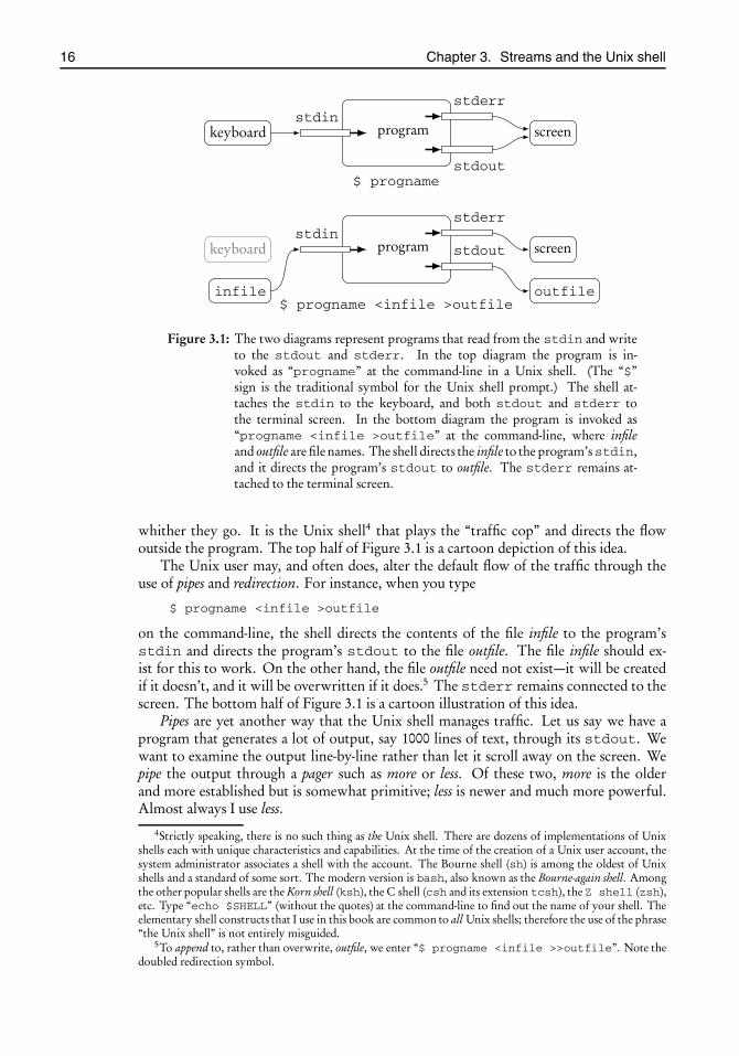
Figure 3.1: The two diagrams represent programs that read from the stdin and writeto the stdout and stderr. In the top diagram the program is in-voked as “progname” at the command-line in a Unix shell. (The “$”sign is the traditional symbol for the Unix shell prompt.) The shell at-taches the stdin to the keyboard, and both stdout and stderr tothe terminal screen. In the bottom diagram the program is invoked as“progname <infile >outfile” at the command-line, where infileand outfile are file names. The shell directs the infile to the program’sstdin,and it directs the program’s stdout to outfile. The stderr remains at-tached to the terminal screen.
whither they go. It is the Unix shell4 that plays the “traffic cop” and directs the flowoutside the program. The top half of Figure 3.1 is a cartoon depiction of this idea.
The Unix user may, and often does, alter the default flow of the traffic through theuse of pipes and redirection. For instance, when you type
$ progname <infile >outfile
on the command-line, the shell directs the contents of the file infile to the program’sstdin and directs the program’s stdout to the file outfile. The file infile should ex-ist for this to work. On the other hand, the file outfile need not exist—it will be createdif it doesn’t, and it will be overwritten if it does.5 The stderr remains connected to thescreen. The bottom half of Figure 3.1 is a cartoon illustration of this idea.
Pipes are yet another way that the Unix shell manages traffic. Let us say we have aprogram that generates a lot of output, say 1000 lines of text, through its stdout. Wewant to examine the output line-by-line rather than let it scroll away on the screen. Wepipe the output through a pager such as more or less. Of these two, more is the olderand more established but is somewhat primitive; less is newer and much more powerful.Almost always I use less.
4Strictly speaking, there is no such thing as the Unix shell. There are dozens of implementations of Unixshells each with unique characteristics and capabilities. At the time of the creation of a Unix user account, thesystem administrator associates a shell with the account. The Bourne shell (sh) is among the oldest of Unixshells and a standard of some sort. The modern version is bash, also known as the Bourne-again shell. Amongthe other popular shells are the Korn shell (ksh), the C shell (csh and its extension tcsh), the Z shell (zsh),etc. Type “echo $SHELL” (without the quotes) at the command-line to find out the name of your shell. Theelementary shell constructs that I use in this book are common to all Unix shells; therefore the use of the phrase“the Unix shell” is not entirely misguided.
5To append to, rather than overwrite, outfile, we enter “$ progname <infile >>outfile”. Note thedoubled redirection symbol.

root2014/7/8page 17
�
�
�
�
�
�
�
�
Chapter 3. Streams and the Unix shell 17
A pager receives a possibly very lengthy text and displays it one-screenful-at-a-timeon the terminal screen. You press the space-bar to display the next screenful. Both moreand less have significantly more features than this—read their man pages for the details—but this should give you an idea of what they do. Invoking the program on the Unixcommand-line as
$ progname <infile |less
directs infile to the progname’s stdin and channels progname’s stdout to less’s stdin.Did you follow that?
Finally, let us address the natural question: why are therestdout andstderr? Whydoes C open two output streams, and why are they treated differently by the Unix shell?
Let us say a part of a program’s computational task involves solving a linear system ofequations and printing the solution or, should the system be singular, printing an errormessage to let the user know of the issue. What is wrong in sending all the program’soutput to the stdout?
What is wrong is this: Should the user redirect the output to a file, then the errormessage will go into that file and possibly escape notice. On the other hand, if the er-ror message is sent to the stderr while the normal output goes out on the stdout,the error message will appear on the screen even when the output is redirected, becauseas we have seen, the shell’s redirection operator “>” redirects the stdout but not thestderr.
It’s the programmer—that’s you—who decides which parts of a program’s outputshould be written tostdout and which to stderr. You will learn that with experience.

root2014/7/8page 19
�
�
�
�
�
�
�
�
Chapter 4
Pointers and arrays
4.1 PointersObjects in C not only have values, but they also have storage locations. For instance, thedeclaration “int i;” associates a memory slot capable of holding an int value withthe identifier i. Setting i = 3 stores a representation of the number 3 in that slot.Printing i, as in “printf("%d\n", i)”, sends i’s value, that is, 3, to the program’sstdout.
The expression &i produces the memory address where i is stored. We may print thataddress as well:
printf("%p\n", (void *)&i);
This will send a numeral such as 0xbf84823c to the stdout.6 The cast to “void *”is necessary because printf()’s %p conversion expects it. The output is likely to varyin every run of the program because there is no reason for i to be stored in the samememory location every time.
The address produced by &i is of type pointer, or in this specific instance, a pointerto int. Although a pointer appears to be of numeric sort, it definitely is not of type int.Objects of type int obey the regular rules of arithmetic, e.g., 1+ 12= 13, while objectsof pointer type don’t. Compare, for instance, the numbers corresponding to &i and1 + &i:
printf("%p\n%p\n", (void *)&i, (void *)(1 + &i));
This will print something like
0xbf84823c0xbf848240
Note that the second number is not 1 plus the first. In fact, it is 4 plus the first. Why 4?It’s because the size (in bytes) of an object of type int in my computer is 4. Adding 1 toa “pointer to int” increments its value by sizeof(int). This generalizes to the funda-mental property of pointer arithmetic:
Adding an integer n to a “pointer to type T” increments the pointer’s valueby n * sizeof(T).
6The 0x prefix signals that this is a hexadecimal (i.e., base 16) representation. Hexadecimal digits are 0, 1,2, . . . , 9, a, b, c, d, e, f.
19

root2014/7/8page 20
�
�
�
�
�
�
�
�
20 Chapter 4. Pointers and arrays
What distinguishes C from many other programming languages is its ubiquitous use ofpointers and pointer arithmetic. A firm grasp of these concepts is essential for benefitingfrom the rest of this book.
4.2 Pointer typesLet p = &i, where i is of type int. We saw in the previous section that although onthe surface the value of p is a number, p is not of type int. Rather, it is of type pointerto int since it is the address of an object of int type. The proper declaration of p is“int *p;”. Note the asterisk.
Thus, p holds the memory address of where i’s value is stored. Since we know theaddress, we should be able to read its contents without referring to i. The expression *pachieves that. In general, if p is a pointer to an object, then *p is the value stored in thatobject.7 The following program accesses and prints the value stored in i, that is, 3, in twodifferent ways: once as i and once as *p. It also prints the address of the object’s locationin two different ways: once as &i and once as p. Try it out and be sure you understandevery detail before moving on.
#include <stdio.h>int main(void){
int i = 3;int *p = &i;printf("value of i = %d, same as %d\n", i, *p);printf("address of i = %p, same as %p\n",
(void *)&i, (void *)p);return 0;
}
In effect, the asterisk (*) and ampersand (&) operators are inverses of each other. Onegoes from value to address; the other goes from address to value. Applying the asteriskoperator to a pointer is called dereferencing the pointer.
4.3 The pointer to voidThe statement “void *p;” declares a special type of pointer called a pointer to void, orvoid pointer. There is no object of type void in C; therefore “void *p;” has no a priorimeaning. C defines it to be a pointer of “generic type” which can point to an object ofany type. This means that the usual pointer arithmetic does not apply to void pointers.What would be the meaning of 1+p, for instance? The pointer arithmetic would want toaddsizeof(void) top, but since there is no object of typevoid, that operation wouldmake no sense. For the same reason, it makes no sense to dereference a void pointer.
The essential property of a void pointer is that it is compatible with all other pointers.The following program illustrates this:
1 #include <stdio.h>2 int main(void)3 {4 int a = 5;5 double x = 3.14;6 void *p;7 p = &a;
7A pointer of type “void *” is an exception. More on that later.

root2014/7/8page 21
�
�
�
�
�
�
�
�
4.4. Arrays 21
8 printf("value of a = %d\n", *(int *)p);9 p = &x;
10 printf("value of x = %g\n", *(double *)p);11 return 0;12 }
In line 7 p is set to hold the address of a, while in line 9 p is set to hold the address of x.This illustrates that a void pointer is generic; it is compatible with assignments to pointersto int and double, or any other type for that matter.
On line 8 we print the contents of the memory location pointed at by p. We notedearlier that a void pointer may not be dereferenced; therefore *p would be illegal. That’swhy we cast p to a pointer to int first and then dereference the result. That shouldexplain the *(int *)p. The cast on line 10 serves a similar purpose.
The genericity of the void pointer enables us to write functions that may admit argu-ments of unspecified types. For instance,
int compare(void *a, void *b);
declares a function named compare() that admits a pair of pointers to objects of any typeas arguments. That function’s implementation may cast and dereference its arguments asappropriate, and return a value less than, equal to, or greater than zero, indicating thatthe first argument is less than, equal to, or greater than the second. Such a function issuitable for passing to the C standard library’s qsort() function, which will sort anarray according to compare()’s criterion. It is crucially important that the argumentsof compare() be generic; otherwise qsort() would be limited to sorting arrays ofonly a fixed type.
4.4 ArraysThe statement “double a[100];” declares an array of length 100 of the type double.This array can hold a sequence of 100 double-precision floating point numbers. The ar-ray’s ith element is a[i]. The array index begins with zero; therefore the array ele-ments are a[0], a[1], a[2], . . . , a[99]. This is in variance with the common usagein mathematics where a vector’s index begins with one; therefore some care is necessarywhen implementing mathematical algorithms in C. Experience shows that this culturaldifference is easy to overcome. The code fragment
double sum = 0.0;for (int i = 0; i < 100; i++)
sum += a[i];
computes the sum of the array’s 100 entries.An array is stored in a contiguous area of the memory; that is, the addresses of the
successive elements of its entries form an arithmetic progression, as illustrated in
#include <stdio.h>int main(void){
double a[4];printf("address of a[0] = %p\n", (void *)&a[0]);printf("address of a[1] = %p\n", (void *)&a[1]);printf("address of a[2] = %p\n", (void *)&a[2]);printf("address of a[3] = %p\n", (void *)&a[3]);return 0;
}
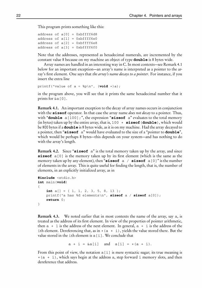
root2014/7/8page 22
�
�
�
�
�
�
�
�
22 Chapter 4. Pointers and arrays
This program prints something like this:
address of a[0] = 0xbffff6d8address of a[1] = 0xbffff6e0address of a[2] = 0xbffff6e8address of a[3] = 0xbffff6f0
Note that the addresses, represented as hexadecimal numerals, are incremented by theconstant value 8 because on my machine an object of type double is 8 bytes wide.
Array names are handled in an interesting way in C. In most contexts—see Remark 4.1below for an important exception—an array’s name is interpreted as a pointer to the ar-ray’s first element. One says that the array’s name decays to a pointer. For instance, if youinsert the extra line
printf("value of a = %p\n", (void *)a);
in the program above, you will see that it prints the same hexadecimal number that itprints for &a[0].
Remark 4.1. An important exception to the decay of array names occurs in conjunctionwith the sizeof operator. In that case the array name does not decay to a pointer. Thus,with “double a[100];”, the expression “sizeof a” evaluates to the total memory(in bytes) taken up by the entire array, that is, 100 * sizeof(double), which wouldbe 800 bytes if a double is 8 bytes wide, as it is on my machine. Had the array decayed toa pointer, then “sizeof a” would have evaluated to the size of a “pointer to double”,which would be perhaps 8 bytes—this depends on your system—and has nothing to dowith the array’s length.
Remark 4.2. Since “sizeof a” is the total memory taken up by the array, and sincesizeof a[0] is the memory taken up by its first element (which is the same as thememory taken up by any element), then “sizeof a / sizeof a[0]” is the numberof elements in the array. This is quite useful for finding the length, that is, the number ofelements, in an explicitly initialized array, as in
#include <stdio.h>int main(void){
int a[] = { 1, 1, 2, 3, 5, 8, 13 };printf("a has %d elements\n", sizeof a / sizeof a[0]);return 0;
}
Remark 4.3. We noted earlier that in most contexts the name of the array, say a, istreated as the address of its first element. In view of the properties of pointer arithmetic,then a + 1 is the address of the next element. In general, a + i is the address of theith element. Dereferencing that, as in *(a + i), yields the value stored there. But thevalue stored in the ith element is a[i]. We conclude that
a + i = &a[i] and a[i] = *(a + i).
From this point of view, the notation a[i] is mere syntactic sugar; its true meaning is*(a + i), which says begin at the address a, step forward i memory slots, and thendereference that address.
root2014/7/8page 23
�
�
�
�
�
�
�
�
4.5. Multidimensional arrays 23
Remark 4.4. The identity a[i] = *(a + i) has a curious consequence:
a[i] = *(a + i) = *(i + a) = i[a].
Therefore, 23[a] is a completely legal—albeit very unorthodox—way of writinga[23].This is hardly more than an amusing curiosity, although some claim that this can be putto good use for writing a more expressive code in certain rare circumstances. For example,since literal strings are treated as arrays in C, bothprintf()s in the program below printthe 7th letter of "Hello World" , that is, W:
#include <stdio.h>int main(void){
printf("%c\n", "Hello World"[6]);printf("%c\n", 6["Hello World"]);return 0;
}
You decide which is the more expressive.
Remark 4.5. Neither*(a + i) nora[i]has built-in error-checking mechanisms. It isyour responsibility as a programmer to make sure that the address a + i lies within thearray’s bounds. Stepping outside the array’s bounds is a fatal error and almost certainlywill crash the program with the dreaded segmentation fault message.
Remark 4.6. There are varying requirements on the declaration of arrays such as“int a[n];” in C89, C99, and C11. In C89, the value of n is required to be a nu-meric constant which is known at the time when the program is compiled. C99 allowsthe value of n to be determined during the program’s execution. Such so-called variable-length arrays proved to be quite unpopular when C99 was announced and raised strongobjections within the C programming community. C11 strikes a compromise by mak-ing the support for variable-length arrays optional. This in effect eliminates the use ofvariable-length arrays in writing portable programs because their support cannot be guar-anteed on all compilers.
For this reason I will refrain from using C99’s variable-length arrays in this book.Dynamically allocated arrays, the topic of Chapter 8, describe the portable way of dealingwith arrays whose sizes are not predetermined.
4.5 Multidimensional arraysThe declaration
double a[3][4];
makes a two-dimensional array that may be used to store a matrix of 3 rows and 4 columns.The element in row i and column j is accessed through the syntax a[i][j]. The expres-sion a[0][2] = 3.14 assigns the value 3.14 to the (0,2) element. Higher-dimensionalarrays work in the same way. For instance, the elasticity tensor of a linearly elastic mate-rial is a 3× 3× 3× 3 array which may be declared as
double C[3][3][3][3];
Its elements will be accessed through the syntax C[i][j][p][q].

root2014/7/8page 24
�
�
�
�
�
�
�
�
24 Chapter 4. Pointers and arrays
4.6 StringsThere is no intrinsic string data type in C. A string is defined to be a contiguous (inmemory) sequence of characters terminated by and including the ASCII NUL character,\0, which is called the string’s null terminator. For instance, the array s[] defined by
char s[8];s[0] = ’T’; s[1] = ’e’; s[2] = ’x’; s[3] = ’t’; s[4] = ’\0’;
represents the string “Text”. The string’s length is 4, but it takes up 5 bytes of storagebecause of the inclusion of the NUL. The array’s elements 5, 6, and 7 are past the nullterminator; therefore they are not a part of the string. Moreover, since they have notbeen assigned to, they will hold garbage values. When we pass a string to a function, weneed not supply the string’s length because the receiving function can tell the string’s endby its null terminator.8
The length and contents of the string defined above may be changed as long as wedon’t exceed the array bounds. For instance,
s[2] = ’s’; s[4] = ’i’; s[5] = ’n’; s[6] = ’g’; s[7] = ’\0’;
changes the string from “Text” to “Testing”.The declaration and initialization steps of a string may be merged into a single state-
ment, as in
char s1[8] = { ’T’, ’e’, ’x’, ’t’, ’\0’ };
or simply:
char s2[] = { ’T’, ’e’, ’x’, ’t’, ’\0’ };
In the latter case, the length of the array will be exactly 5.It is also possible to define a string simply as
char s3[] = "Text";
or
char *s4 = "Text";
Any of the strings s1 · · · s4 may be used with identical results in most contexts wherestrings are used—all four represent “Text”. However, there are subtle differences that oneneeds to be aware of, especially in relation to the sizeof operator, as can be seen here:
#include <stdio.h>int main(void){
char s1[8] = { ’T’, ’e’, ’x’, ’t’, ’\0’ };char s2[] = { ’T’, ’e’, ’x’, ’t’, ’\0’ };char s3[] = "Text";char *s4 = "Text";
printf("s1 = %s, sizeof s1 = %d\n", s1, sizeof s1);printf("s2 = %s, sizeof s2 = %d\n", s2, sizeof s2);printf("s3 = %s, sizeof s3 = %d\n", s3, sizeof s3);printf("s4 = %s, sizeof s4 = %d\n", s4, sizeof s4);return 0;
}
8Old joke floating on the Internet: These two strings walk into a bar and sit down. The bartendersays, “So what’ll it be?” The first string says, “I think I’ll have a beer fulk boorg jdk@¿ÇjfdŁ¡ kjk3sd#f67hower89åøvyo. . . “Please excuse my friend,” the second string says, “she isn’t null-terminated.”
root2014/7/8page 25
�
�
�
�
�
�
�
�
4.7. The command-line arguments 25
This prints
s1 = Text, sizeof s1 = 8s2 = Text, sizeof s2 = 5s3 = Text, sizeof s3 = 5s4 = Text, sizeof s4 = 4
Can you explain the result? Recall the discussion of the decay of array names and theexception noted in Remark 4.1 on page 22.
Remark 4.7. A quoted set of characters, such as the "Text" in the definition of s3 ands4 above, is called a string literal. Your C compiler is permitted to treat a string literal asa read-only object, making it impossible to change its letters. For instance, with the s1and s4 defined as above, setting s1[0] = ’N’ is quite legal and changes s1 to “Next”,but setting s4[0] = ’N’ is illegal and may have unpredictable results.
The C standard library provides a dozen or so functions for working with strings.There are functions to copy, concatenate, search, compare, tokenize, and print strings.For instance the strlen() function gives a string’s length (not counting the null termi-nator.)
4.7 The command-line argumentsPrograms are often invoked with command-line arguments and options. For instance,the Unix utility diff takes two file names as arguments, as in diff file1 file2,and prints the differences between the contents of the two files. How are the file namesfile1 and file2 conveyed from the command-line to the diff program?
C provides two alternative forms for declaring the function main(). If the pro-gram has no use for command-line arguments, then we use the simpler alternative,“int main(void)”. If the program needs to access the command-line arguments,then we use the second alternative: “int main(int argc, char **argv)”.In the latter case, the argc parameter will hold the number of command-line to-kens with which the program is invoked. For instance, if the command-line is“diff file1 file2”, then the value of argc will be set to 3. If a program is invokedwith no arguments, then the only command-line token is the program’s name; thereforeargc is set to 1.
The argv parameter is an array of length argc + 1 of pointers to char; argv[0]points to a string corresponding to the first command-line token, which is the name ofthe program; argv[1] through argv[argc-1] point to strings corresponding to theremaining command-line tokens; argv[argc] is the NULL pointer—it marks the end ofthe argv array much in the same way that the null terminator marks the end of a string.Figure 4.1 is a schematic representation of the idea.
The following program prints the command-line arguments and exits:
#include <stdio.h>int main(int argc, char **argv){
while (*argv �= NULL)printf("%s\n", *argv++);
return 0;}
Can you think of other ways of doing this?

root2014/7/8page 26
�
�
�
�
�
�
�
�
26 Chapter 4. Pointers and arrays
argv[0]
argv[1]
argv[2]
NULL
argv d i f f \0
f i l e 1 \0
f i l e 2 \0
Figure 4.1: The schematic representation of the memory layout of the command-linearguments when the program is invoked as “diff file1 file2”.
Remark 4.8. This section’s discourse on the values of argc and argv is intentionallysimplistic and not quite accurate. My aim has been to cover the most common case, andin that sense what I have written is accurate. It is possible, however, to step outside ofthe ordinary and encounter behaviors which are quite at odds with what I have said. Forinstance, Unix’s exec() family of functions allows one to execute a program in such away that argc appears to be zero or in such way that argc is nonzero but argv[0] issomething other than the program’s name. These issues are not of relevance to this book’smaterial; therefore I will not go into them.

root2014/7/8page 27
�
�
�
�
�
�
�
�
Chapter 5
From strings to numbers
In Section 4.7 we saw how to access the user-supplied command-line arguments as stringsargv[0], argv[1], etc. If any of these arguments is supposed to be interpreted asa number, then we need a means of converting a string to a number. The C standardlibrary provides several functions for that purpose. In this chapter we will learn about afew of these which are used frequently in the rest of this book.
5.1 The function strtod()
The standard library’s strtod() (think of it as string to double) function “converts theinitial portion of a string” to a number of type double. The expression in the quotes,which comes from the C standard, requires some explanation. The function is declaredin the standard header file stdlib.h as
double strtod(const char *nptr, char **endptr);
We see that it takes two arguments. The first argument is expected to be a pointerto a string that expresses a floating point number such as “3.14”, “-0.123”, or“6.0221415e+23”. Leading whitespace, if any, is ignored. The parsing of the stringstops when the end of the number is detected. Thus, the string may include trailing junk.For instance, “ 6.022e+23xyz” yields the same number as “6.022e+23”. HereI have used “ ” to mark whitespace characters.
The second argument, called the end-pointer, is the address of a pointer tochar. Uponreaching the end of the numeric portion of the string, strtod() sets the end-pointerto point to the memory location next to the number’s last character. For instance, ifthe string is “6.022e+23xyz”, then the end-pointer points to the character “x”. Inparticular, if there is no trailing junk, then the end-pointer points to the string’s nullterminator, that is, the “\0” character. It follows that if, after strtod() returns, the end-pointer is pointing to anything other than “\0”, then the string contains trailing junk. It’sconceivable that the user put the junk there on purpose, but more often than not, trailingjunk is the result of an unintended error in the input—perhaps a slip of the finger on thekeyboard—and we would want to catch that. Therefore, a typical call to strtod() takesthe form
#include <stdlib.h>char *str = ...; // some string herechar *endptr;
27
root2014/7/8page 28
�
�
�
�
�
�
�
�
28 Chapter 5. From strings to numbers
double x;x = strtod(str, &endptr);if (*endptr �= ’\0’)
fprintf(stderr, "your string has trailing junk!\n");else
printf("the number is %g\n", x);
Remark 5.1. The standard library also provides strtof() and strtold(), whichreturn floating point numbers of types float and long double, respectively. Thefunction strtod() dates back to C89. The other two were added in C99. We will haveuse only for strtod() in this book.
5.2 The function strtol()
The standard library’s strtol() (think of it as string to long int) function “converts theinitial portion of a string” to a number of type long int. The expression in the quotescomes from the C standard which, in the header file stdlib.h, declares the prototype:
long int strtol(const char *nptr, char **endptr, int base);
We see that strtol() takes three arguments. The first argument is expected to be astring that expresses an integer such as “123”, “-321”, or “beef” (yes, that’s a hex-adecimal number). Initial whitespace, if any, is ignored. The parsing of the string stopswhen the end of the number is detected. Thus, the string may include trailing junk. Forinstance, “ -321#@x” yields the same number as “-321”.
The second argument, called the end-pointer, works exactly like that in the case ofstrtod() described in the previous section; therefore I will not repeat that descrip-tion here. The third argument is the base in which the number is to be interpreted. Fordecimal numbers the base is 10. For hexadecimal numbers it is 16. The base may be assmall as 2 (a binary number) or as large as 35. The digits in base 35 are 0,1, . . . , 9,a, b , . . . , z(uppercase or lowercase letters are equivalent). Setting the base to zero has a special mean-ing which is not worth getting into in this brief overview. Read your C reference to findout if you are curious.
Here is a typical call to strtol():
#include <stdlib.h>char *str = ...; // some string herechar *endptr;long int n;n = strtol(str, &endptr, 10);if (*endptr �= ’\0’)
fprintf(stderr, "your string has trailing junk!\n");else
printf("the number is %d\n", n);
Remark 5.2. The standard library also provides the function strtoll()which returnsextended range integers of the type long long int. You may use strtoll() to findout the base 10 equivalent of the hexadecimal number deadbeef. On a typical computerit is likely that deadbeef is beyond the range of long int, so strtol() won’t do.
There are alsostrtoul() and strtoull()which return unsigned long intand unsigned long long int. The functions strtol() and strtoul() date

root2014/7/8page 29
�
�
�
�
�
�
�
�
5.3. The functions atof(), atol(), and friends 29
back to C89. The other two were added in C99. We will have use only for strtol() inthis book.
5.3 The functions atof(), atol(), and friendsThe C standard library function atof() (think of it as ascii to float) is the lazy man’sversion of strtod(). It is declared in stdlib.h as
double atof(const char *nptr);
Thus, atof() takes a pointer to a string and produces a floating point number of typedouble. Initial whitespace and trailing junk, if any, are silently ignored. Therefore,atof( 6.022e+23xyz) returns 6.022e+23.
The C standard library function atol() (think of it as ascii to long int) is the lazyman’s version of strtol(). It is declared in stdlib.h as
long int atol(const char *nptr);
Thus, it takes a pointer to a string and produces an integer of type long int. Initialwhitespace and trailing junk, if any, are silently ignored. Therefore, atol( -321xyz)returns -321. Unlike strtol(), there is no provision for bases other than 10.
There are also atoi() and atoll() which work just like atol() but return intand long long int, respectively. The functions atof(), atol(), and atoi() dateback to C89. The function atoll() was introduced in C99.
This section’s ato*() functions can be handy for quick-and-dirty jobs and throw-away programs. For a work of any permanence, I recommendstrtod() andstrtol().We won’t use the ato*() functions in this book.

root2014/7/8page 31
�
�
�
�
�
�
�
�
Chapter 6
Make
6.1 Multifile programsIt helps to split a program into as many logically independent parts as possible. Generallya small programming unit is easier to comprehend, debug, and improve. A “logicallyindependent part” does not stand in vacuum, however. It is always connected throughthin filaments to the other parts; otherwise one could remove it and nothing would bethe worse for it.
The “parts” of the program generally manifest themselves as files or groups of files.Programs that are spread over dozens, if not hundreds, of files are quite common. Unix’smake utility is an essential tool for managing a multipart program.
To provide a context to this exposition, I will refer to Chapter 17’s Project Evolution,although a knowledge of the details of that chapter is not a prerequisite for understand-ing this chapter. Project Evolution is spread over five *.c files and six *.h files:9
$ cd evolution$ ls -Farray.h@ read.c world-to-eps.h [email protected] read.h write.c [email protected] world-to-eps.c write.h
It’s possible to compile the entire program via a single command:10
$ gcc -Wall -pedantic -std=c99 -O2 evolution.c read.c \world-to-eps.c write.c xmalloc.c -o evolution
Indeed, this will compile the five *.c files and produce an executable file named “evolu-tion”; the -o flag precedes the name of the desired executable. The *.h files are not listedexplicitly; the compiler inserts them where indicated by the preprocessor’s #includedirectives.
6.2 Separate compilation and linkingThe single-line compilation method works, but it’s rather primitive and is hardly ever ad-visable. If you edit one of the files, say write.c, then of course you will have to recompile it,
9Files decorated with “@” are symbolic links, as explained in Chapter 2.10I have broken the line in two, as it is too long to fit between the margins of this book. A backslash (\) at
the end of a Unix command-line indicates that the line is continued into the next. See Section 1.5 regarding thecompilation flags -Wall -pedantic -std=c99 -O2.
31
root2014/7/8page 32
�
�
�
�
�
�
�
�
32 Chapter 6. Make
but there should be no need to recompile the rest of the *.c files if you haven’t touchedthem. The sensible thing to do is to compile the files individually, and when a particularfile changes, then recompile just that one, leaving the rest alone. Here is how that’s done:
$ gcc -c -Wall -pedantic -std=c99 -O2 evolution.c$ gcc -c -Wall -pedantic -std=c99 -O2 read.c$ gcc -c -Wall -pedantic -std=c99 -O2 world-to-eps.c$ gcc -c -Wall -pedantic -std=c99 -O2 write.c$ gcc -c -Wall -pedantic -std=c99 -O2 xmalloc.c
The -c flag tells gcc to compile each *.c file into a corresponding *.o file, called an objectfile. Although an object file is a finished product as far as compilation goes, it’s not suitablefor stand-alone execution since it’s only a fragment of a whole program. Consider, forinstance, the first of the five lines shown above. Within evolution.c there is a referenceto the function read_world_def() which is defined elsewhere (in read.c, to be exact).The header file read.h, which is #included in evolution.c, reassures the compiler thatthe function read_world_def()with a specific prototype will be made available later.That satisfies the compiler, and it produces the object file evolution.o with a danglingreference to the promised read_world_def().
There are many more dangling references in evolution.o. In evolution.c there are sev-eral references to the function printf(), for instance, which is defined elsewhere (inthe C standard library, to be exact). The header file stdio.h, which is #included in evo-lution.c, reassures the compiler that the function printf() with a specific prototypewill be made available later.
The loose ends are tied together in a process called linking. It’s done by giving thenames of the object files to gcc, as in
$ gcc evolution.o read.o world-to-eps.o write.o xmalloc.o \-o evolution
Again I have broken the long line in two, but you can see what is going on. There are nocompilation flags, such as -Wall, because no compilation takes place here. Gcc sees alist of object files and recognizes the request for linking. It ties the loose ends among thelisted *.o files and the standard library, and produces the executable file named “evolution”because that’s what the -o flag tells it.
Suppose we make a change in write.c. Producing a new executable amounts to
$ gcc -c -Wall -pedantic -std=c99 -O2 write.c$ gcc evolution.o read.o world-to-eps.o write.o xmalloc.o \
-o evolution
That is, we recompile write.c and relink. The other *.c files were not touched; thereforethey need not be recompiled.
6.3 File dependenciesThis is all quite straightforward until we change a header file, say write.h. Which files needto be recompiled now? We need to inspect each of the other *.c and *.h files to find outwhich of them #includes the file write.h and then recompile the affected files. Doingthis manually can be daunting because a program’s various files may be interrelated incomplex ways. Figure 6.1 shows the dependencies of the files in Project Evolution. At thevery top is the executable evolution which depends on the five *.o files. We see that theobject file write.o depends on write.h, write.c, and evolution.h. We also see that the objectfile evolution.o depends on evolution.c as well as the six header files *.h.

root2014/7/8page 33
�
�
�
�
�
�
�
�
6.3. File dependencies 33
evolution.h read.h write.h xmalloc.hwrite-to-eps.harray.h
evolution.o read.o write.o xmalloc.owrite-to-eps.o
evolution.c read.c write.c xmalloc.cwrite-to-eps.c
evolution
Figure 6.1: This diagram shows the dependency tree among the files pertaining toProject Evolution. The executable evolution (at top) depends on the *.o filesin the second row. Each of the *.o files depends on one or more *.c and *.hfiles, listed at the bottom two rows.
Fortunately, we don’t have to discover these dependencies through laborious manualinspection; gcc’s -MM flag will do that for us. In response to the command
$ gcc -MM evolution.c read.c world-to-eps.c write.c xmalloc.c
it prints
evolution.o: evolution.c evolution.h xmalloc.h array.h read.h \write.h world-to-eps.h
read.o: read.c xmalloc.h read.h evolution.hworld-to-eps.o: world-to-eps.c world-to-eps.h evolution.hwrite.o: write.c write.h evolution.hxmalloc.o: xmalloc.c xmalloc.h
Each line has the form “target: dependency1 dependency2 . . . ”. For instance, we see thatwrite.o depends on write.c, write.h, and evolution.h, as was noted earlier. Item or items tothe left of the colon are called targets. Item or items to the right of the colon are calleddependencies.
The form of the output of gcc -MM is designed specifically to mesh with the Unixutility called make. Make reads a file, usually called Makefile, that contains the list oftargets/dependencies of a project in the textual form shown above. It then figures outwhat needs to be done to compile the program without further human intervention.
You, the programmer, write the appropriate Makefile for your program. Writing aMakefile may seem akin to black magic if you don’t know the principles behind it. In thenext several sections I will construct a sequence of Makefiles, initially some rather prim-itive ones and then progressively more sophisticated and complex ones but with greaterutility. The later versions are much more practical, and I recommend that you use thoserather than the simplistic early versions, but don’t skip over the earlier versions as you readthis chapter; they show the progression of logic that leads to the somewhat complex finalproduct which may not be easily decipherable otherwise.
root2014/7/8page 34
�
�
�
�
�
�
�
�
34 Chapter 6. Make
Listing 6.1: Makefile version 1. Make recognizes a backslash \ at the end of a line as a directive tocontinue to the next line, as the Unix shell does.
1 evolution: evolution.o read.o world-to-eps.o write.o xmalloc.o2 gcc evolution.o read.o world-to-eps.o write.o xmalloc.o \3 -o evolution4
5 evolution.o: evolution.c evolution.h xmalloc.h array.h read.h \6 write.h world-to-eps.h7 gcc -Wall -pedantic -std=c99 -O2 evolution.c8
9 read.o: read.c xmalloc.h read.h evolution.h10 gcc -Wall -pedantic -std=c99 -O2 read.c11
12 world-to-eps.o: world-to-eps.c world-to-eps.h evolution.h13 gcc -Wall -pedantic -std=c99 -O2 world-to-eps.c14
15 write.o: write.c write.h evolution.h16 gcc -Wall -pedantic -std=c99 -O2 write.c17
18 xmalloc.o: xmalloc.c xmalloc.h19 gcc -Wall -pedantic -std=c99 -O2 xmalloc.c
6.4 Makefile version 1The first version of our Makefile shown in Listing 6.1 is quite verbose but also quite simpleto comprehend. Line 1 says that the target file called “evolution” depends on the five *.ofiles shown. That single line is exactly equivalent to the top half of Figure 6.1.
As it stands, line 1 is incomplete: it asserts what the target depends on but does nottell how to build it from its dependencies. We, the humans, know that it’s done throughlinking:
$ gcc evolution.o read.o world-to-eps.o write.o xmalloc.o \-o evolution
but make doesn’t know that and needs to be told. That’s where line 2 comes in. In aMakefile we may associate a command with a target/dependency pair. The command tellsmake what needs to be done to produce the target out of the dependencies. The syntax is
target : dependencies
commandtab
The tab that precedes the command is a literal Tab character and is absolutely essential;spaces won’t do. The GNU make’s manual thus puts it emphatically: “You need to puta tab character at the beginning of every command line! This is an obscurity that catchesthe unwary.”
Equipped with this knowledge, you should have no problems in deciphering theMakefile of Listing 6.1. Line 15, for instance, says that write.o depends on write.c, write.h,and evolution.h. Line 16 supplies the command that produces write.o out of thosedependencies. The indentation of that line is due to the presence of the leading tab.

root2014/7/8page 35
�
�
�
�
�
�
�
�
6.6. Makefile version 2 35
6.5 How to run make
At this point we have a file named Makefile whose contents are shown in Listing 6.1.Execute the Unix command
$ make
and—voilà!—make reads and executes the instructions in the Makefile and produces thefile evolution. What is even more impressive, if you change any of your source files andrun make again, it will detect what has changed and will know exactly which files torecompile—since it knows their interdependencies—to create a new evolution file. If yourerun make without having made any changes, it will know that there is nothing to doand will tell you so.
Remark 6.1. Occasionally it is useful to run make with the -n flag:
$ make -n
This does a “dry run”—it prints out what will be done without doing them.
Let us look once more at the Makefile in Listing 6.1. Note that there are six targetsin it. When we run make, it picks up the very first target to build. It sees that the firsttarget, that is, evolution, depends on evolution.o among other things. So it looks up andexecutes the instructions for building evolution.o. It repeats this for the other *.o files andthen puts them together to build the first target.
In view of the special role of a Makefile’s first target, it is a good idea to put the mostfrequently needed object as the first target in a Makefile. This is not absolutely necessary,however. Had we placed the evolution target somewhere else, let’s say at the end of theMakefile, we still could have requested make to build it by giving the name of the targetexplicitly on the command-line:
$ make evolution
Putting the most frequently needed object as the first target in a Makefile makes life a littleeasier since it won’t be necessary to type the target’s name on the command-line.
6.6 Makefile version 2Line 16 of Listing 6.1 instructs make to compile write.c in order to build write.o. Butthat’s rather obvious; how else would one build write.o out of write.c? Can’t make figurethat out by itself? It turns out that yes, it can! Make has a built-in rule for producing anobject file from a C file. If we don’t specify the command ourselves, make will apply thebuilt-in rule. This means that line 16 is superfluous and may be removed.
There remains an issue regarding gcc’s compilation options. If we remove line 16,then how do we tell make to compile write.c with our favorite compilation flags?
Make recognizes a built-in variable named CFLAGS. We may define CFLAGS in theMakefile as we wish. Make will apply CFLAGS along with its built-in compilation rules.Implementing these observations, we arrive at version 2 of our Makefile shown in List-ing 6.2. Relative to the previous version, I have removed the commands associated withthe *.o targets to let make apply its own built-in rules instead. Note the CFLAGS definedat the top.
Lines 3 and 4 have remained exactly as before because we still need to tell make how tobuild the evolution target from the object files. That part is very much project-dependent;no built-in rule can help there.

root2014/7/8page 36
�
�
�
�
�
�
�
�
36 Chapter 6. Make
Listing 6.2: Makefile version 2.
1 CFLAGS = -Wall -pedantic -std=c99 -O22
3 evolution: evolution.o read.o world-to-eps.o write.o xmalloc.o4 gcc evolution.o read.o world-to-eps.o write.o xmalloc.o \5 -o evolution6
7 evolution.o: evolution.c evolution.h xmalloc.h array.h read.h \8 write.h world-to-eps.h9 read.o: read.c xmalloc.h read.h evolution.h
10 world-to-eps.o: world-to-eps.c world-to-eps.h evolution.h11 write.o: write.c write.h evolution.h12 xmalloc.o: xmalloc.c xmalloc.h
Remark 6.2. Lines from 7 on down are exactly what “gcc -MM” produces (see theoutput shown on page 33); therefore one does not type those lines by hand. I certainlydidn’t.
There are several ways to grab the output of “gcc -MM” and stick it into the Makefile.If you are working on a terminal that allows copying and pasting with the mouse, youmay do just that, that is, copy the output of “gcc -MM” and paste it into the Makefile,but that is probably the clumsiest way of doing it. A better way is to rely on your Unixshell’s redirection ability to append11 gcc’s output to the Makefile:
$ gcc -MM evolution.c read.c world-to-eps.c \write.c xmalloc.c >>Makefile
You should remember, however, as you add and remove files, or change any #includelines in your sources, or anything else that may alter the file dependency tree, you need torefresh those dependency lines. To do that, edit the Makefile, delete the previous depen-dency lines, and then regenerate them as instructed above.
There are ways to automate the updating of the dependency lines in a Makefile butthey will probably be more confusing to a beginner than of help, so I won’t go there.
6.7 Makefile version 3There is something disconcerting about version 2 of the Makefile in Listing 6.2: line 4repeats the file names from line 3. That’s rather annoying because any change in oneline requires the identical change in the other. To avoid repetition, we introduce a newvariable, let’s call it OFILES,12 that declares the names of the object files:
OFILES = evolution.o read.o world-to-eps.o write.o xmalloc.o
Then we may refer to that variable instead of listing the object files explicitly. To refer toOFILES, we write $(OFILES). Thus, lines 3 and 4 simplify to
evolution: $(OFILES)gcc $(OFILES) -o evolution
Can it be made any simpler? Yes, it can! The word “evolution” appears in two places.We may avoid the repetition by changing the above to
11See the remark in footnote 5 on page 16.12Unlike CFLAGS, which is a make built-in, the name “OFILES” has no special significance; you may call it
as you wish. Many programmers use “OBJS” for this purpose.

root2014/7/8page 37
�
�
�
�
�
�
�
�
6.7. Makefile version 3 37
evolution: $(OFILES)gcc $(OFILES) -o $@
The “$@” is an internal variable in make that holds the name of the associated target. Thechoice of the symbol “@” is apropos since it looks so much like a target/bull’s-eye.
Let us remark that we have managed to reduce the bulky first three lines of Makefileversion 1 (see Listing 6.1 on page 34) to a quite simple and almost generic two-liner. Itwould be even more generic if could we get rid of the occurrence of the word “evolution”there as well. In fact, we can. Let us define a new variable, let’s call it TARGET, as in
TARGET = evolution
Then the previous block of code changes to
$(TARGET): $(OFILES)gcc $(OFILES) -o $@
To make this completely generic, we change gcc to $(CC). The latter is defined to ex-pand to the name of your system’s default C compiler. On most Linux machines $(CC)expands to cc, which is a link to gcc. If your system is equipped with multiple C com-pilers, then you may define CC in your Makefile, as in
CC = icc
which tells make to use Intel’s C compiler, icc, instead of the default.13 With this finalchange, we arrive at
$(TARGET): $(OFILES)$(CC) $(OFILES) -o $@
Hooray! This is completely generic! There are no references there to any specific projector any compiler; therefore this fragment of the Makefile will be the same in all projects.We celebrate this achievement by making version 3 of our Makefile, shown in Listing 6.3.In effect, only the first two lines in that Makefile are project-dependent. Everything elseis generic. I am not counting the material that appears below line 8 since that is automat-ically generated by “gcc -MM”.
Remark 6.3. The “#” character in a Makefile signals the beginning of a comment. Makeignores everything from there to the end of line. The entire line 8 of Listing 6.3 is acomment.
Remark 6.4. Up to this point I have adhered strictly to the syntax and semantics oforiginal make, which dates back to 1977. You should expect that any implementation ofthe make utility—and there are quite a few—should respect the Makefiles constructed upto this point, and should process them as intended.
The more recent versions of make add features of their own as extensions to the orig-inal make. One of the more popular implementations, the GNU make, adds a “$^”internal variable which expands to the list of a target’s dependencies. Thus, the secondoccurrence of $(OFILES) in the previous code snippet may be replaced by “$^”, as in
$(TARGET): $(OFILES)$(CC) $^ -o $@
13Compiler flags vary wildly from one compiler to another. If you switch to another compiler, you may haveto change CFLAGS accordingly.

root2014/7/8page 38
�
�
�
�
�
�
�
�
38 Chapter 6. Make
Listing 6.3: Makefile version 3.
1 OFILES = evolution.o read.o world-to-eps.o write.o xmalloc.o2 TARGET = evolution3 CC = gcc4 CFLAGS = -Wall -pedantic -std=c99 -O25 $(TARGET): $(OFILES)6 $(CC) $(OFILES) -o $@7
8 # below this is the output of "gcc -MM":9 evolution.o: evolution.c evolution.h xmalloc.h array.h read.h \
10 write.h world-to-eps.h11 read.o: read.c xmalloc.h read.h evolution.h12 world-to-eps.o: world-to-eps.c world-to-eps.h evolution.h13 write.o: write.c write.h evolution.h14 xmalloc.o: xmalloc.c xmalloc.h
There is not much of an advantage in using “$^” in this particular instance, but it can bequite handy in a Makefile that builds multiple executables, e.g.,
target1: file1.o file2.o$(CC) $^ -o $@
target2: file3.o file4.o$(CC) $^ -o $@
You will have to balance the convenience of using “$^” against the possible lack of porta-bility.
6.8 Makefile: The final versionThe program for Project Evolution consists of five *.c files and six *.h files. Compiling theprogram adds five *.o files as well as the executable which we have named evolution. Oc-casionally you will want to “clean up” the directory by removing all machine-generatedfiles, leaving only the original source files. You want to do that when sending your pro-gram to someone else—there is no point in sending object files and executables since theseare specific to your operating system. Such a cleanup is also helpful when you wish torecompile the entire program from scratch and watch for any compiler warnings that youmay have missed earlier.
We may remove the object file and executables in Project Evolution through the Unixcommand-line
$ rm evolution.o read.o world-to-eps.o write.o \xmalloc.o evolution
but that’s too tedious and error-prone, especially if we have a large number of files. Wemay enlist make to help us here as well. Note that the parameters given to the “rm ...”command above are exactly what were called $(OFILES) and $(TARGET) in our Make-file. Therefore, within the Makefile, that command takes the form
rm $(OFILES) $(TARGET)

root2014/7/8page 39
�
�
�
�
�
�
�
�
6.8. Makefile: The final version 39
Listing 6.4: Makefile, final version. Only the first two lines are project-dependent. Everything elseis generic. I am not counting the material that appears toward the end because that isautomatically generated by “gcc -MM”.
1 OFILES = evolution.o read.o world-to-eps.o write.o xmalloc.o2 TARGET = evolution3 CC = gcc4 CFLAGS = -Wall -pedantic -std=c99 -O25 $(TARGET): $(OFILES)6 $(CC) $(OFILES) -o $@7
8 clean:9 rm -f $(OFILES) $(TARGET)
10
11 # below this is the output of "gcc -MM":12 evolution.o: evolution.c evolution.h xmalloc.h array.h read.h \13 write.h world-to-eps.h14 read.o: read.c xmalloc.h read.h evolution.h15 world-to-eps.o: world-to-eps.c world-to-eps.h evolution.h16 write.o: write.c write.h evolution.h17 xmalloc.o: xmalloc.c xmalloc.h
Where do we put that line in the Makefile? We make up a “phony” target, let’s callit “clean”, which has no dependencies and whose associated command performs theremoval:
clean:rm $(OFILES) $(TARGET)
As we noted in Section 6.5, typing “make” on the command-line with no argumentspicks up the very first target in the Makefile. To pick up some other target, we give it as anargument to make. Thus, to reach the “clean” target, on the Unix command-line we type
$ make clean
This will work fine, but it can be improved. It’s true that the command “make clean”will remove $(OFILES) and $(TARGET), as intended, but executing the command“make clean” for a second time will elicit a complaint from rm since there will beno such files to remove. The -f flag suppresses such complaints from rm:
clean:rm -f $(OFILES) $(TARGET)
Remark 6.5. Our use of the target “clean” constitutes an abuse of themake utility. Makeis designed with the assumption that targets will be actual file names, but “clean” is nota file name; it’s a phony target. This is not an issue unless for some reason you happento have a file named “clean” in the same directory. That will confuse make to no end.The generic solution is to avoid having a file named “clean”, or if you must, then considerchanging the name of the target to something else, like “cleanup”. A solution specific toGNU make is to explicitly declare clean a “phony target”. Look up the Phony Targetssection in GNU make’s manual if you are interested.
We add the “clean” target to our Makefile and arrive at the final version shown inListing 6.4. Admittedly, calling it the “final version” is somewhat premature: it is missing

root2014/7/8page 40
�
�
�
�
�
�
�
�
40 Chapter 6. Make
important features such as a means to link with external libraries. Nevertheless, what wehave here is a good foundation to build upon, as we will see in the following sections.
6.9 Linking with external librariesWe will have several occasions in this book to link our programs with third-party libraries.For instance, the finite element solver of Chapter 25 relies on the Triangle library to tri-angulate the domain, the UMFPACK library to solve the resulting linear system, and thestandard library’s mathematics library for mathematical functions, such as sqrt(). Tolink with these libraries, we pass the-ltriangle -lumfpack -lm flags to the linker.A good way of doing this in a Makefile is to define
LIBS = -ltriangle -lumfpack -lm
and then change the command that performs the linking to
$(TARGET): $(OFILES)$(CC) $(OFILES) $(LIBS) -o $@
6.10 Multiple executables in one MakefileIn Project Nelder–Mead of Chapter 18 we write several independent demonstration pro-grams named demo-1D, demo-2D, demo-energy, demo-constrained, etc. Here are the rulesto build the first two:
OFILES_1D = xmalloc.o nelder-mead.o demo-1D.oOFILES_2D = xmalloc.o nelder-mead.o demo-2D.o
demo-1D: $(OFILES_1D)$(CC) $(OFILES_1D) -o $@
demo-2D: $(OFILES_2D)$(CC) $(OFILES_2D) -o $@
If demo-1D is the first target, then the command make, with no arguments, willbuild the executable demo-1D. To produce the remaining executables, we will have to givetheir names on the command-line, as in “make demo-2D”, “make demo-energy”,“make demo-constrained”, etc. This can be irksome if we have to rebuild the tar-gets repeatedly. Fortunately, a simple trick can automate the building of any number oftargets with a single command. Listing 6.5 shows how.
There we define the variable ALL as the list of the desired executables. As the Make-file’s first target we define a phony target called all which depends on $(ALL). Thus,entering make on the command-line picks up that first target, that is, all. Since alldepends on the list of executables, building all amounts to building all the executables.

root2014/7/8page 41
�
�
�
�
�
�
�
�
6.10. Multiple executables in one Makefile 41
Listing 6.5: This is a typical Makefile for building multiple executables. Entering the commandmake on the command-line will pick the first target, all, which depends on $(ALL),which in turns is the list of the desired executables.Note: If you are willing to use GNU make’s $^ extension (see Remark 6.4),then you may simplify this Makefile by replacing every “$(CC) ...” line with“$(CC) $^ -o $@”.
OFILES_RANK_VERTICES = rank-vertices-test.oOFILES_1D = xmalloc.o nelder-mead.o demo-1D.oOFILES_2D = xmalloc.o nelder-mead.o demo-2D.oOFILES_ENERGY = xmalloc.o nelder-mead.o demo-energy.oOFILES_CONSTRAINED = xmalloc.o nelder-mead.o demo-constrained.o
CFLAGS = -Wall -pedantic -std=c99 -O2
ALL = rank-vertices-test demo-1D demo-2D demo-energy demo-constrained
all: $(ALL)
rank-vertices-test: $(OFILES_RANK_VERTICES)$(CC) $(OFILES_RANK_VERTICES) -o $@
demo-1D: $(OFILES_1D)$(CC) $(OFILES_1D) -o $@
demo-2D: $(OFILES_2D)$(CC) $(OFILES_2D) -o $@
demo-energy: $(OFILES_ENERGY)$(CC) $(OFILES_ENERGY) -o $@ -lm
demo-constrained: $(OFILES_CONSTRAINED)$(CC) $(OFILES_CONSTRAINED) -o $@
clean:rm -f $(ALL) $(OFILES_RANK_VERTICES) $(OFILES_1D) $(OFILES_2D) \
$(OFILES_ENERGY) $(OFILES_CONSTRAINED)
# the output of "gcc -MM" goes here...

root2014/7/8page 45
�
�
�
�
�
�
�
�
Chapter 7
Allocating memory:xmalloc()
Prerequisites: None
7.1 IntroductionThe C standard library’s malloc() function, declared in the header file stdlib.h, allocatesa contiguous block of memory of the requested size (in bytes) and returns a void pointer(cf. Section 4.3) that points to the beginning of the block. The request may fail if therequested amount is greater than what’s available. In that case malloc() returns NULL.
The action to take when malloc() fails is dictated by the nature of the application.For instance, if a text editing program runs out of memory, the proper action wouldbe to notify the user of the fact and give him the opportunity to save the work beforeexiting. Similarly, if the overnight execution of a lengthy scientific computation runs outof memory, it would be prudent that it saves its current state before quitting, so that itmay be resumed later from where it was cut off rather than starting anew. At the otherextreme, if the program has nothing worthwhile to save, then the proper action would beto issue an alert and then quit.
All of this book’s programs fall in the latter category. Therefore we introduce a functionmalloc_or_exit() that serves as a front end to malloc(). It calls malloc() andchecks the result. If NULL, then it prints a diagnostic to the stderr and calls exit() toterminate the program. Otherwise it returns the result to the caller. By implementing thiswrapper around malloc(), we are freeing the user of the responsibility of checking ex-plicitly for malloc()’s success—if the program is still alive after malloc_or_exit()returns, then malloc() must have succeeded. This simplifies and streamlines our pro-grams substantially.
Furthermore, we introduce a function-like preprocessor macro, xmalloc(), whichoffers a simplified interface to malloc_or_exit(), as we shall see below. All memoryallocation in the rest of this book is done through the xmalloc() macro.
7.2 A review of malloc()Our xmalloc module relies on the standard library’s malloc() function for allocatingmemory. A typical usage of malloc() is shown in Listing 7.1. There are quite a fewideas there, so let us go through it line by line (but not necessarily in sequential order).
45
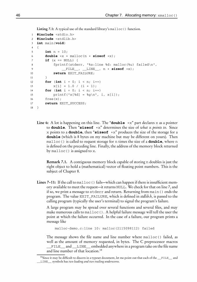
root2014/7/8page 46
�
�
�
�
�
�
�
�
46 Chapter 7. Allocating memory: xmalloc()
Listing 7.1: A typical use of the standard library’s malloc() function.
1 #include <stdio.h>2 #include <stdlib.h>3 int main(void)4 {5 int n = 10;6 double *x = malloc(n * sizeof *x);7 if (x == NULL) {8 fprintf(stderr, "%s:line %d: malloc(%u) failed\n",9 __FILE__, __LINE__, n * sizeof *x);
10 return EXIT_FAILURE;11 }12 for (int i = 0; i < n; i++)13 x[i] = 1.0 / (i + 1);14 for (int i = 0; i < n; i++)15 printf("x[%d] = %g\n", i, x[i]);16 free(x);17 return EXIT_SUCCESS;18 }
Line 6: A lot is happening on this line. The “double *x” part declares x as a pointerto double. Then “sizeof *x” determines the size of what x points to. Sincex points to a double, then “sizeof *x” produces the size of the storage for adouble (which is 8 bytes on my machine but may be different on yours). Thenmalloc() is called to request storage for n times the size of a double, where nis defined on the preceding line. Finally, the address of the memory block returnedby malloc() is assigned to x.
Remark 7.1. A contiguous memory block capable of storing n doubles is just theright object to hold a (mathematical) vector of floating point numbers. This is thesubject of Chapter 8.
Lines 7–11: If the call tomalloc() fails—which can happen if there is insufficient mem-ory available to meet the request—it returns NULL. We check for that on line 7, andif so, we print a message to stderr and return. Returning from main() ends theprogram. The value EXIT_FAILURE, which is defined in stdlib.h, is passed to thecalling program (typically the user’s terminal) to signal the program’s failure.
A large program may be spread over several functions and several files, and maymake numerous calls to malloc(). A helpful failure message will tell the user thepoint at which the failure occurred. In the case of a failure, our program prints amessage like
malloc-demo.c:line 10: malloc(2115098112) failed
The message shows the file name and line number where malloc() failed, aswell as the amount of memory requested, in bytes. The C preprocessor macros__FILE__ and __LINE__ embedded anywhere in a program take on the file nameand line number of that location.14
14Since it may be difficult to discern in a typeset document, let me point out that each of the __FILE__ and__LINE__ symbols has two leading and two trailing underscores.

root2014/7/8page 47
�
�
�
�
�
�
�
�
7.2. A review of malloc() 47
Line 12: We fill the allocated space with the sequence of numbers { 1i+1 }n−1
i=0 . Note thatthe pointer x is being treated exactly like a C array. How is that?
The answer lies in the pointer arithmetic of Section 4.1. For one thing, x pointsto the beginning of the allocated memory block. For another thing, since x isa pointer to double, adding i to x will move forward by “i times the size ofdouble” bytes in the memory space. Thus, “*(x + i)” will represent thevalue stored in the ith position. Accordingly, line 13 could have been written as“*(x + i) = 1.0 / (i + 1);”. However, *(x + i) is the same as x[i],as we noted on page 22. This explains the form of line 13.
Remark 7.2. What we have learned here is that memory allocated by malloc()may be handled with a syntax identical to that of the built-in C arrays, althoughthe two are quite different objects as far as C goes. What makes the identical syntaxpossible is the clever design of the pointer arithmetic.
Line 14: We go through the allocated memory and print out its contents. There is noth-ing new here, but observe again that the syntax to access the content of the ithlocation is just as if x were an ordinary C array.
Line 16: We call free(), which is declared in stdlib.h along with malloc(), to releasethe memory that was procured by malloc(). A well-designed program will haveas many calls to free() as there are calls to malloc(). In fact, the allocatedmemory should be freed as soon as it is no longer needed so that the program mayreclaim it for other use. There is no reason to hog a system resource if it’s no longerneeded.15
Modern operating systems automatically release all memory allocated by a pro-gram when the program terminates. In such systems, releasing memory explicitlyjust before the exit is redundant. Nevertheless, a fastidious attention to releasing allallocated memory before leaving the program is the mark of an experienced pro-grammer, much in the same way that cleaning up the area before striking the tentis an indicator of a conscientious camper. There are tangible benefits as well, otherthan just making you feel good about yourself. Experience shows that attention tothe details of allocation and freeing memory imposes a certain self-discipline whichultimately results in better structured and more elegant programs. Furthermore, ifit happens that your program is imbedded later in a larger program, the place whereyour program used to exit is no longer a point of exit of the larger program. If yourprogram does not clean up after itself, it can wreak havoc with the larger program.
As a case in point, think of your program as a solver of a static partial differentialequation and the larger program as a time-stepper that simulates an evolving dy-namics. At every one of the thousands of time-steps, the time-stepper calls yourprogram to update its state. A memory leak in your program can bring the largerprogram to a halt. I know; I am speaking from experience.
Valgrind from <http://valgrind.org/> is an open source free software that cancheck your program for memory leaks. Invoked at the command-line as
$ valgrind your-program’s-name your-program’s-arguments
15This is especially important for programs that run over extended periods of time, such as web browsers,system daemons, and servers. Memory allocated and abandoned without freeing can grow over time and bringthe system to standstill. Programs that suffer from this malady are said to “leak memory”.

root2014/7/8page 48
�
�
�
�
�
�
�
�
48 Chapter 7. Allocating memory: xmalloc()
it will run the program under its control, and at the end will print a report indicat-ing the number of times your program called malloc() and free() and whetherthere was a memory leak.
You will find an extensive discussion of memory management issues in Chapter 8 ofC Unleashed [27]. You may be interested in the memtrack utility described thereto track memory allocation and release in a complex program.
Line 17: The value of EXIT_SUCCESS, defined in stdlib.h, is passed to the calling pro-gram (typically the user’s terminal shell) to signal the program’s successful termina-tion. Returning EXIT_SUCCESS from main() is equivalent to returning 0. Themacro EXIT_SUCCESS exists for symmetry with the macro EXIT_FAILURE.There is no standard numerical code corresponding to the latter.
Line 1: The functions printf() and fprintf() are declared in the header file stdio.h.
Line 2: The functions malloc() and free(), as well as the macros EXIT_SUCCESSand EXIT_FAILURE, are declared in the header file stdlib.h.
Line 5: The value of n, defined here as 10, is used in the argument to malloc() anda couple of other places in the program. It is important to note that n need nothave been a preassigned constant. With a little more effort, we could have arrangedthings so that the program would read the value of n from the command-line, forexample. The point is, the vector x need not have a predetermined length. This isvery much in contrast to C’s native arrays, which can only have a priori fixed sizes.See Remark 4.6 on page 23 for details.
7.3 The programThis chapter’s xmalloc module facilitates allocating and freeing memory, and is used forthat purpose in almost every chapter in the rest of this book. The files xmalloc.h andxmalloc.c constitute the module’s interface and implementation. The files xmalloc-demo-1.c and xmalloc-demo-2.c are two drivers for demonstrating some of the uses and featuresof the module. This project’s directory contains
$ cd xmalloc$ ls -Fxmalloc-demo-1.c xmalloc-demo-2.c xmalloc.c xmalloc.h
We may automate the compilation with the help of a Makefile along the lines of the in-structions in Chapter 6, but the current demos are so small that writing a Makefile forthem may be an overkill. To compile them manually, we do
$ gcc -c -Wall -pedantic -std=c99 -O2 xmalloc.c$ gcc -c -Wall -pedantic -std=c99 -O2 xmalloc-demo-1.c$ gcc xmalloc.o xmalloc-demo-1.o -o xmalloc-demo-1$ gcc -c -Wall -pedantic -std=c99 -O2 xmalloc-demo-2.c$ gcc xmalloc.o xmalloc-demo-2.o -o xmalloc-demo-2
The only reason for specifying -std=c99 is the use of the fprintf()’s%zu conversionspecifier for printing values of type size_t. The z specifier was introduced in C99. Seethe discussion on page 6 for the C89 alternative.

root2014/7/8page 49
�
�
�
�
�
�
�
�
7.4. The interface and the implementation 49
Here is the transcript of an interactive session with the first demo:
$ ./xmalloc-demo-1allocating 1000 bytesmemory freedallocating 0 bytesxmalloc-demo-1.c:line 18: malloc(0) failed
As we see, the program allocates 1000 bytes successfully and then frees it. Next, it attemptsto allocate 0 bytes. Our program refuses such a request (what does it mean to allocate0 bytes?), so it prints a diagnostic message and exits. (See Part 7.1 of Section 7.5 for moreon this.)
Here is the transcript of an interactive session with the second demo:
./xmalloc-demo-21: 1000000000 bytes allocated2: 1000000000 bytes allocated
� (the next 140730 lines deleted)140734: 1000000000 bytes allocated140735: 1000000000 bytes allocatedxmalloc-demo-2.c:line 10: malloc(1000000000) failed
This demo allocates memory chunks of 1,000,000,000 bytes (1 gigabyte) in an unendingwhile-loop without freeing them. It prints a line upon each pass through the loop. Afterstepping through the loop 140,735 times, my computer’s memory is exhausted; thereforethe program exits with a diagnostic.
Does my computer truly have 140,735 gigabytes of memory? Not a chance! Whatwe see here is a Linux artifact—I am running this program on a computer with a 64-bitLinux operating system—which allocates memory generously in a virtual memory spacefar beyond what is physically available, in the hope that not all of the requested memorywill actually be needed. Under a more conservative operating system the program mayhave stopped in fewer than 8 iterations since I have only 8 gigabytes of physical memoryon this computer.
7.4 The interface and the implementationThe xmalloc module is needed in almost all of this book’s projects; therefore I expectthat every reader will go through this chapter early in their studies. For that reason,I will devote more than the usual amount of attention to details here. In particular, in thefollowing two subsections I will present essentially the entire contents of the files xmalloc.cand xmalloc.h. You will make a slight adjustment to my xmalloc.c in the Projects section.
7.4.1 xmalloc.c: The implementation
Listing 7.2 gives a preliminary version of the file xmalloc.c which implements our xmallocmodule. It defines a function malloc_or_exit()which receives, as its first argument,the number of bytes of memory to be allocated, and as the second and third argumentsthe file name and line number whence it was invoked. If the allocation is successful, itreturns a pointer to the start of the allocated memory; otherwise it prints a message ofthe sort
foo.c:line 123: malloc() of 10000 bytes failed
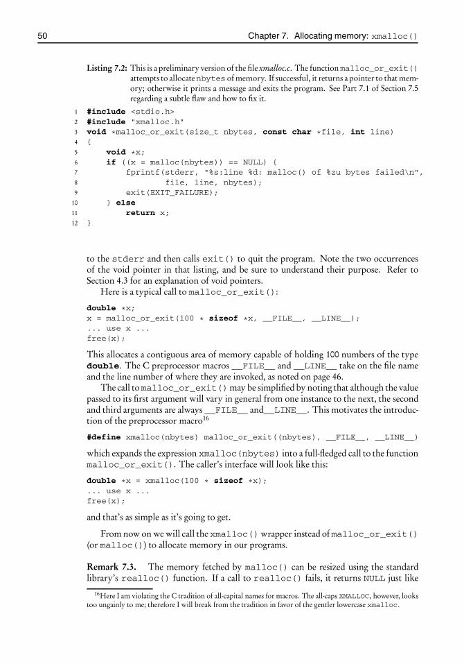
root2014/7/8page 50
�
�
�
�
�
�
�
�
50 Chapter 7. Allocating memory: xmalloc()
Listing 7.2: This is a preliminary version of the file xmalloc.c. The functionmalloc_or_exit()attempts to allocatenbytes of memory. If successful, it returns a pointer to that mem-ory; otherwise it prints a message and exits the program. See Part 7.1 of Section 7.5regarding a subtle flaw and how to fix it.
1 #include <stdio.h>2 #include "xmalloc.h"3 void *malloc_or_exit(size_t nbytes, const char *file, int line)4 {5 void *x;6 if ((x = malloc(nbytes)) == NULL) {7 fprintf(stderr, "%s:line %d: malloc() of %zu bytes failed\n",8 file, line, nbytes);9 exit(EXIT_FAILURE);
10 } else11 return x;12 }
to the stderr and then calls exit() to quit the program. Note the two occurrencesof the void pointer in that listing, and be sure to understand their purpose. Refer toSection 4.3 for an explanation of void pointers.
Here is a typical call to malloc_or_exit():
double *x;x = malloc_or_exit(100 * sizeof *x, __FILE__, __LINE__);... use x ...free(x);
This allocates a contiguous area of memory capable of holding 100 numbers of the typedouble. The C preprocessor macros __FILE__ and __LINE__ take on the file nameand the line number of where they are invoked, as noted on page 46.
The call tomalloc_or_exit()may be simplified by noting that although the valuepassed to its first argument will vary in general from one instance to the next, the secondand third arguments are always __FILE__ and__LINE__. This motivates the introduc-tion of the preprocessor macro16
#define xmalloc(nbytes) malloc_or_exit((nbytes), __FILE__, __LINE__)
which expands the expression xmalloc(nbytes) into a full-fledged call to the functionmalloc_or_exit(). The caller’s interface will look like this:
double *x = xmalloc(100 * sizeof *x);... use x ...free(x);
and that’s as simple as it’s going to get.
From now on we will call the xmalloc()wrapper instead of malloc_or_exit()(or malloc()) to allocate memory in our programs.
Remark 7.3. The memory fetched by malloc() can be resized using the standardlibrary’s realloc() function. If a call to realloc() fails, it returns NULL just like
16Here I am violating the C tradition of all-capital names for macros. The all-caps XMALLOC, however, lookstoo ungainly to me; therefore I will break from the tradition in favor of the gentler lowercase xmalloc.

root2014/7/8page 51
�
�
�
�
�
�
�
�
7.4. The interface and the implementation 51
Listing 7.3: The header file xmalloc.h provides the xmalloc module’s interface.
1 #ifndef H_XMALLOC_H2 #define H_XMALLOC_H3 #include <stdlib.h>4 void *malloc_or_exit(size_t nbytes, const char *file, int line);5 #define xmalloc(nbytes) malloc_or_exit((nbytes), __FILE__, __LINE__)6 #endif /∗ H_XMALLOC_H */
malloc(); therefore for completeness it would be useful to have an xrealloc() toaccompany xmalloc(). However, we don’t have a use for realloc() in this book;therefore I will not explore that idea any further.
7.4.2 xmalloc.h: The interface
The header file xmalloc.h, shown in its entirety in Listing 7.3, provides the interface toour xmalloc module. A few comments on its structure are in order:
Lines 1, 2, and 6: These are the header file’s so-called header guards or #include guards.Their purpose is to prevent unintended multiple inclusions of this header file inother units. To illustrate a case of multiple inclusion in the absence of #includeguards, consider two header files header1.h and header2.h and a program file prog.cthat #includes both of them. If header2.h also #includes header1.h, thenheader1.h will be read twice into prog.c, leading to potential complications.
If a header file is equipped with #include guards, as is our xmalloc.h, then this iswhat happens. When xmalloc.c #includes xmalloc.h for the first time, line 1determines that the symbol H_XMALLOC_H is undefined; therefore control passesto line 2, where H_XMALLOC_H gets defined. The rest of xmalloc.h is read as usual.
Should xmalloc.c attempt to #include xmalloc.h for a second time, line 1 willdetermine that the symbol H_XMALLOC_H is already defined; therefore control willpass to line 6, thus bypassing the main body of xmalloc.h.
Every header file should be equipped with #include guards. The guard symbol, which isH_XMALLOC_H in our case, is arbitrary, but it should be unique within all headerfiles of the entire project. The usual way of creating such a unique symbol is bybasing it on the name of the corresponding header file. Since our header file isnamed xmalloc.h, any of the choices XMALLOC, XMALLOC_H, H_XMALLOC_H, orvariations thereof, will serve the purpose. The second one is the traditional choicein C. I prefer the third one since the leading H avoids an (admittedly remote) clashwith IEEE’s POSIX standard, which reserves symbol names beginning with E forits own use.
The comment on line 6 is not required; its sole purpose is to remind one that the#endif on that line corresponds to the #ifndef H_XMALLOC_H on line 1. Ina short header file such as our xmalloc.h, this is rather superfluous, but in a headerfile that spans hundreds of lines, the reminder is a nice touch.
Remark 7.4. It is a common beginner’s mistake to name the #include guard sym-bols with a leading underscore, such as _XMALLOC, mimicking those in the C stan-dard library. The C standard, however, reserves preprocessor symbols that begin

root2014/7/8page 52
�
�
�
�
�
�
�
�
52 Chapter 7. Allocating memory: xmalloc()
with an underscore for its own private use. If you name your symbols with a lead-ing underscore, you run the risk of stepping over your compiler’s internals. That’svery bad. Don’t do it!
Line 3: At first sight it may look odd why we have #include <stdlib.h> in xmal-loc.h while #include <stdio.h> in xmalloc.c. The reason for including stdio.hin xmalloc.c is to provide a prototype for fprintf() that occurs in that file. Thereis no fprintf() in xmalloc.h and hence no need for stdio.h there. On the otherhand, we include stdlib.h in xmalloc.h because it defines the symbol size_t whichis needed in xmalloc.h.17 There is yet another—and not so obvious—minor benefit ofincluding stdlib.h in xmalloc.h. Programs that call xmalloc() to allocate memoryeventually will call free() to release that memory. When they include xmalloc.h,they receive stdlib.h (which declares the prototype of free()) as a bonus; thereforethey need not include it separately.
7.5 Project Xmalloc
Part 7.1. The function malloc_or_exit() in Listing 7.2 allocates nbytes bytesof memory and returns that memory’s address. But what should it return if nbytes iszero? The C99 standard has the following to say:
Section 7.20.3: If the size of the space requested is zero, the behavior isimplementation-defined: either a null pointer is returned, or the behavioris as if the size were some nonzero value, except that the returned pointershall not be used to access an object.
In short, allocating zero bytes is ill-defined, so we might as well treat it just as whenmalloc() fails. Modify malloc_or_exit() to account for this.
Part 7.2. Implement the adjustment suggested in the previous part. Then write a pro-gram, let’s say xmalloc-demo-1.c, that does the following:
1. calls xmalloc() to allocate 1000 bytes of memory and then prints a message say-ing that the memory was allocated;
2. frees that memory and then prints a message saying that the memory was freed;
3. calls xmalloc() to allocate 0 bytes of memory and then prints a message sayingthat the memory was allocated; and
4. frees that memory and then prints a message saying that the memory was freed.
Will the program print 4 lines? See the transcript of the interactive session on page 49.
Part 7.3. Write a program, let’s say xmalloc-demo-2.c, that allocates memory in chunksof 1,000,000,000 bytes (1 gigabyte) and abandons them (that is, does not free them), ina nonterminating (infinite) loop. Print a message on each pass. Will the program runforever? See the transcript of the interactive session on page 49.
17The symbolsize_t is also defined in the standard header file stddef.h; therefore one could include it insteadof stdlib.h if the only objective were to define size_t.

root2014/7/8page 53
�
�
�
�
�
�
�
�
Chapter 8
Dynamic memoryallocation for vectorsand matrices: array.h
Prerequisite: Chapter 7
8.1 IntroductionIn this chapter we introduce a preprocessor trick to construct vectors, matrices—and evenhigher-dimensional array-like objects—in a type-generic way in standard C.18 The prepro-cessor macro make_matrix(), for instance, constructs a matrix of any type. Thus, toconstruct 5× 7 matrices of the types int, double, and “struct point”, we do
int **a;double **x;struct point {double x; double y;} **p;int m = 5, n = 7;make_matrix(a, m, n);make_matrix(x, m, n);make_matrix(p, m, n);x[0][0] = 3.14159; // use x, etc.free_matrix(a);free_matrix(x);free_matrix(p);
Observe how the three matrices of varying types are constructed and freed through anidentical interface. There is also a make_vector() to construct type-generic vectors,and make_3array() and make_4array() to construct type-generic three- and four-dimensional arrays. All these are bundled in a header file named array.h. There is noassociated array.c file.
Preprocessor macros are not the most elegant part of the C programming language,and they are best avoided if the job can be done without them. Unfortunately, type-generic construction of arrays, as laid out above, is impossible in C89 and C99 withoutthe help of preprocessor macros since C lacks polymorphism. On the balance, the ab-solutely simple user-interfaces and the versatility of these macros far outweigh the some-what ungainly code that resides in array.h. At any rate, what we have here is better thanany alternatives of which I know. We rely on the macros provided in array.h throughoutthe rest of this book to create and destroy vectors and matrices. Thankfully, we won’thave to look inside array.h every time we use it.
18The trick works equally well in C89 and C99.
53

root2014/7/8page 54
�
�
�
�
�
�
�
�
54 Chapter 8. Dynamic memory allocation for vectors and matrices: array.h
8.2 Constructing vectors of arbitrary typesThe xmalloc() wrapper of Chapter 7 provides a convenient way for creating vectorsof various lengths and types. With simple wrappers such as19
int *make_ivector(size_t n) // provisional{
int *v = xmalloc(n * sizeof *v);return v;
}double *make_dvector(size_t n) // provisional{
double *v = xmalloc(n * sizeof *v);return v;
}
we may call make_ivector(n) and make_dvector(n) to make vectors of length nof the types int and double.
If this were the end of the story, the functions above could justly be criticized ongrounds that they make things more complicated than necessary. After all, allocatingmemory for a vector of n double-precision floating point numbers can be as simple as
double *v = malloc(n * sizeof *v);
where make_dvector() and xmalloc() don’t come into the play at all. However,this is not the end of the story. What we have so far is an infrastructure upon whichwe are going to build extensively. The significance of this will become apparent whenwe construct type-generic vectors, matrices, and higher-dimensional arrays later in thischapter.
Before doing that, however, let us revisit the two functions defined above. There issomething unsatisfactory in their approach since, continuing along those lines, we willneed to write a special-purpose vector allocation function for every new data type thatcomes along. That’s annoying, particularly since the number of potential data types isinfinite. It would be more elegant having a single function capable of constructing vectorsof all types. Although such a function is infeasible—there is no polymorphism in C—theequivalent effect is achieved easily through a function-like preprocessor macro
#define make_vector(v,n) ((v) = xmalloc((n) * sizeof *(v)))
which is type-agnostic and may be used to allocate memory for vectors of any type.20 Inthe following code fragment, we apply the make_vector() macro to make a vector oflength 100 of type double:
double *x;make_vector(x, 100);for (int i = 0; i < 100; i++)
x[i] = 1.0 / (1 + i);free_vector(x);
In the next example, we apply the same make_vector() macro to make a vector oflength 30 of type “struct point”:
19I have marked these functions “provisional” since the make_vector() macro, to be introduced shortly,does the same job and much more!
20The plethora of parentheses in this macro definition is standard fare. Consult the chapter on preprocessormacros in your C reference book for an explanation. Also see footnote 16 on page 50 regarding a break withtradition.

root2014/7/8page 55
�
�
�
�
�
�
�
�
8.2. Constructing vectors of arbitrary types 55
struct point {double x; double y;} *p;make_vector(p, 30); // make a vector of 30 pointsp[0]→x = 3.14; p[0]→y = 2.78; // define p[0]’s coordinatesp[1]→x = 12.1; p[1]→y = -0.3; // define p[1]’s coordinates... etc. ...free_vector(p);
What is free_vector()? It frees the memory allocated by make_vector(). Inprinciple, freeing that memory is a matter of calling the standard library’s free(), asin “free(x)” or “free(p)” in the two examples above. Nevertheless, we introducethe free_vector() macro as a simple wrapper around free(p), for the sake of sym-metry with make_vector(). And as long as we are at it, we go one step further andarrange things so that after freeing the memory, the corresponding pointer is set to NULL.This is an unnecessary and insignificant frill, but there are those who are passionate aboutNULL-ing freed pointers. This should please them:
#define free_vector(v) do { free(v); v = NULL; } while (0)
The free(v) and v = NULL parts require no explanation, but the do and while(0)would definitely look strange if you are seeing this well-known construction for the firsttime. Let me explain.
Preprocessor macros consisting of multiple statements must be handled with care.Consider a hypothetical macro consisting of two statements:
#define bad_macro statement1; statement2
Then observe that the code fragment
if (test1)bad_macro;
elsesomething_else;
expands to
if (test1)statement 1;statement 2;
elsesomething_else;
which is syntactically incorrect—braces are missing. Adding braces to the macro
#define bad_macro { statement1; statement2; }
does not help because now the code fragment expands to
if (test1) {statement 1;statement 2;
}; elsesomething_else;
which is still incorrect—the semicolon before the else shouldn’t be there. However,setting
#define good_macro do { statement1; statement2; } while (0)

root2014/7/8page 56
�
�
�
�
�
�
�
�
56 Chapter 8. Dynamic memory allocation for vectors and matrices: array.h
a[0]
a[1]
a[2]
NULL
a a[0][0] a[0][1] a[0][2] a[0][3] a[0][4]
a[1][0] a[1][1] a[1][2] a[1][3] a[1][4]
a[2][0] a[2][1] a[2][2] a[2][3] a[2][4]
pointer to the“pointer vector”
the “pointer vector”
Figure 8.1: The schematic representation of the memory layout for a 3×5 matrix. The“pointer vector” that appears as a vertical column on the left is a vector ofpointers to the matrix’s rows.
does the trick. The while(0) condition ensures that the block inside the braces is exe-cuted exactly once. The code fragment expands to
if (test1)do {
statement 1;statement 2;
} while (0);else
something_else;
which is just right.
8.3 A scheme for dynamically allocated matricesFigure 8.1 is a schematic representation of memory layout for a dynamically allocated3 × 5 matrix. The matrix rows are viewed as vectors of length 5 obtained by calls tomake_vector(). The addresses of the first elements of those vectors are stored in a“column” vector of length 4 shown along the diagram’s left edge. We call that the pointervector because its elements are pointers to the row vectors. The last element of the pointervector is set to NULL; it serves as a sentinel that marks the end of the vector. CompareFigure 8.1 with Figure 4.1 on page 26 concerning C’s storage scheme for the command-linearguments. They reflect identical ideas.
The identifier a, which serves as the name of the matrix, holds the address of thepointer vector’s first element. Since the elements of the pointer vector are pointers, thena is a pointer to pointer.
The elements of the pointer vector are a[i], i = 0, . . . , 3; therefore the address ofthe ith row is a[i], and hence the values stored in that row are a[i][j]. We see thatsuch dynamically allocated matrices and C’s native two-dimensional arrays have identicalsyntax for addressing the matrix’s elements. However, their internal storage and repre-sentations can be entirely different. Matrices constructed here should not be confused withC’s native two-dimensional arrays.
The provisional21 make_dmatrix() function defined below implements the schemedescribed above for constructing an m× n matrix of type double:
21I have marked this function “provisional” since the make_matrix() macro developed in the next sectiondoes the same job and much more!
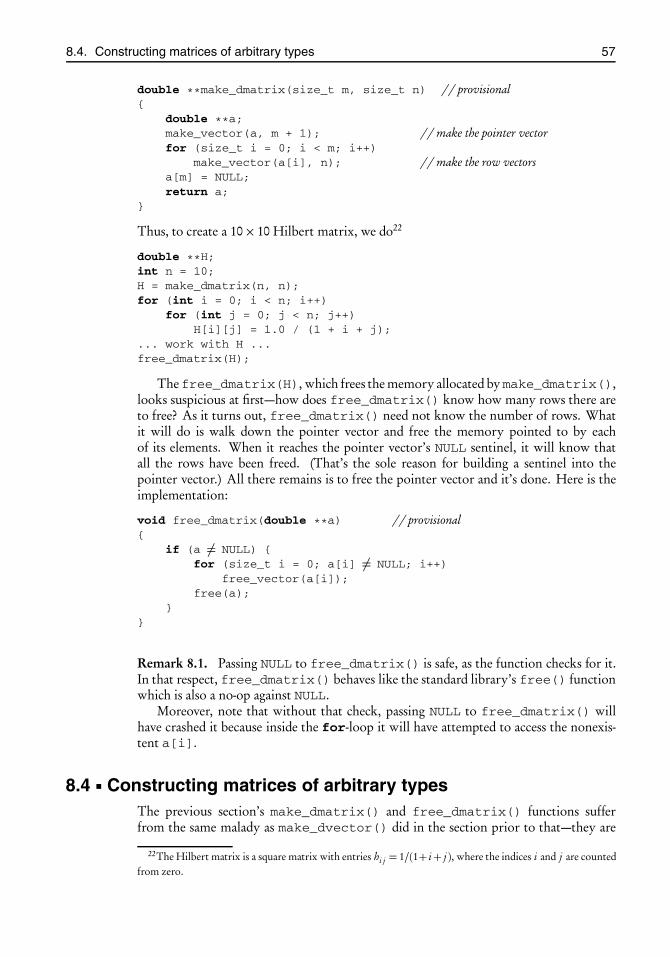
root2014/7/8page 57
�
�
�
�
�
�
�
�
8.4. Constructing matrices of arbitrary types 57
double **make_dmatrix(size_t m, size_t n) // provisional{
double **a;make_vector(a, m + 1); // make the pointer vectorfor (size_t i = 0; i < m; i++)
make_vector(a[i], n); // make the row vectorsa[m] = NULL;return a;
}
Thus, to create a 10× 10 Hilbert matrix, we do22
double **H;int n = 10;H = make_dmatrix(n, n);for (int i = 0; i < n; i++)
for (int j = 0; j < n; j++)H[i][j] = 1.0 / (1 + i + j);
... work with H ...free_dmatrix(H);
Thefree_dmatrix(H), which frees the memory allocated bymake_dmatrix(),looks suspicious at first—how does free_dmatrix() know how many rows there areto free? As it turns out, free_dmatrix() need not know the number of rows. Whatit will do is walk down the pointer vector and free the memory pointed to by eachof its elements. When it reaches the pointer vector’s NULL sentinel, it will know thatall the rows have been freed. (That’s the sole reason for building a sentinel into thepointer vector.) All there remains is to free the pointer vector and it’s done. Here is theimplementation:
void free_dmatrix(double **a) // provisional{
if (a �= NULL) {for (size_t i = 0; a[i] �= NULL; i++)
free_vector(a[i]);free(a);
}}
Remark 8.1. Passing NULL to free_dmatrix() is safe, as the function checks for it.In that respect, free_dmatrix() behaves like the standard library’s free() functionwhich is also a no-op against NULL.
Moreover, note that without that check, passing NULL to free_dmatrix() willhave crashed it because inside the for-loop it will have attempted to access the nonexis-tent a[i].
8.4 Constructing matrices of arbitrary typesThe previous section’s make_dmatrix() and free_dmatrix() functions sufferfrom the same malady as make_dvector() did in the section prior to that—they are
22The Hilbert matrix is a square matrix with entries hi j = 1/(1+ i+ j ), where the indices i and j are countedfrom zero.

root2014/7/8page 58
�
�
�
�
�
�
�
�
58 Chapter 8. Dynamic memory allocation for vectors and matrices: array.h
limited to constructing and freeing matrices of the type double. To make a matrix ofthe type int, for instance, we will have to write another version.
In Section 8.2 we overcame the problem in the case of vectors with the help of a pre-processor macro. In this section we extend that preprocessor trick to matrices. This isquite straightforward other than the issue of handling the loop counter i in the func-tion make_dmatrix() defined on page 57. The scope of that counter is limited tothe body of the function, and as such it is invisible to the outside world. Convert-ing the function to a preprocessor macro, however, exposes its innards and poses a po-tential for a clash between its loop counter and another identifier of the same namewhich may be lurking in the code. The way around this is to use a reserved identi-fier name instead of a generic i and alert the macro’s users23 of its presence. I call thecounter “make_matrix_loop_counter” since the close association with the name“make_matrix” makes it unlikely that a user will encroach upon it inadvertently. Withthis out of the way, here is the promised macro:
#define make_matrix(a, m, n) do { \size_t make_matrix_loop_counter; \make_vector(a, (m) + 1); \for (make_matrix_loop_counter = 0; \
make_matrix_loop_counter < (m); \make_matrix_loop_counter++) \
make_vector((a)[make_matrix_loop_counter], (n)); \(a)[m] = NULL; \
} while (0)
In the same way, we convert the function free_dmatrix() to a macro:
#define free_matrix(a) do { \if (a �= NULL) { \
size_t make_matrix_loop_counter; \for (make_matrix_loop_counter = 0; \
(a)[make_matrix_loop_counter] �= NULL; \make_matrix_loop_counter++) \
free_vector((a)[make_matrix_loop_counter]); \free_vector(a); \a = NULL; \
} \} while (0)
The backslashes (“\”) indicate line continuation in a preprocessor macro. I have alignedthem vertically purely for aesthetic reasons; they don’t have to be aligned. I have used thereserved identifier make_matrix_loop_counter in both macros; there is no reasonto introduce two different reserved words. Additionally, I have added a = NULL at theend of free_matrix() for the same reason we did so in the case of free_vector().
On the surface, these macros are ungainly. Nevertheless they are quite general andoffer particularly clean interfaces, and ultimately that’s what matters. Here is the previoussection’s Hilbert matrix, constructed with the help of make_matrix():
double **H;int n = 10;make_matrix(H, n, n); // was H = make_dmatrix(n, n);
23The “users” includes you!

root2014/7/8page 59
�
�
�
�
�
�
�
�
8.5. Project array.h 59
Listing 8.1: An outline of the file array.h.
1 #ifndef H_ARRAY_H2 #define H_ARRAY_H3 #include "xmalloc.h"4 � #define make_vector(...5 � #define free_vector(...6 � #define make_matrix(...7 � #define free_matrix(...8 #endif /∗ H_ARRAY_H */
for (int i = 0; i < n; i++)for (int j = 0; j < n; j++)
H[i][j] = 1.0 / (1 + i + j);... work with H ...free_matrix(H);
Only one line (as marked) has changed relative to the previous version.
8.5 Project array.hCreate a directory, say vector-and-matrix, to hold this chapter’s material. Our macrosrely on Chapter 7’s xmalloc module for allocating memory. If you organize your files assuggested in Chapter 2, your directory will look like this:
$ cd vector-and-matrix$ ls -Farray.h hilbert-matrix.c xmalloc.c@ xmalloc.h@
where the “@” decoration at the end of a file name indicates a symbolic link, as explainedin Chapter 2. The details of the files array.h and hilbert-matrix.c are described below.
Part 8.1. Put the definitions of the macros make_vector(), free_vector(),make_matrix(), and free_matrix() in a file array.h, and add #include guards, asshown in an outline form in Listing 8.1. See page 51 regarding the significance of #includeguards.
Part 8.2. Listing 8.2 provides an outline of a file named hilbert-matrix.c. In it we havea function named hilbert_matrix() which constructs and returns the address of ann × n Hilbert matrix for a given n. (See footnote 22 on page 57 for the definition of aHilbert matrix.) The function hilbert_matrix() is called from within main() tobuild an 8×8 Hilbert matrix. The program exits after printing the matrix and freeing theallocated memory.
Supply the details, compile, and execute the program. Its should print something likethis:1.000 0.500 0.333 0.250 0.200 0.167 0.143 0.1250.500 0.333 0.250 0.200 0.167 0.143 0.125 0.1110.333 0.250 0.200 0.167 0.143 0.125 0.111 0.1000.250 0.200 0.167 0.143 0.125 0.111 0.100 0.0910.200 0.167 0.143 0.125 0.111 0.100 0.091 0.0830.167 0.143 0.125 0.111 0.100 0.091 0.083 0.0770.143 0.125 0.111 0.100 0.091 0.083 0.077 0.0710.125 0.111 0.100 0.091 0.083 0.077 0.071 0.067

root2014/7/8page 60
�
�
�
�
�
�
�
�
60 Chapter 8. Dynamic memory allocation for vectors and matrices: array.h
Listing 8.2: An outline of hilbert-matrix.c.
� the necessary #includesdouble **hilbert_matrix(int n){� call make_matrix() to make and return theaddress of an nxn Hilbert matrix
}int main(void){
double **H;int n = 8;H = hilbert_matrix(n);� print the matrix� free the matrixreturn 0;
}
Listing 8.3: A type-generic implementation of the preprocessor macro print_vector(). Weuse the symbol print_vector_loop_counter for a loop counter. The users ofthis macro should be told that this is a reserved word and should not be interfered with.
#define print_vector(fmt, v, n) do { \size_t print_vector_loop_counter; \for (print_vector_loop_counter = 0; \
print_vector_loop_counter < (n); \print_vector_loop_counter++) \
printf(fmt, (v)[print_vector_loop_counter]); \putchar(’\n’); \
} while (0)
Listing 8.4: Code fragment showing a sample usage of the print_vector()macro. This shouldprint “ 1.000 0.500 0.333 0.250 0.200”.
double *v;int i, n = 5;make_vector(v, n);for (i = 0; i < n; i++)
v[i] = 1.0 / (1 + i);print_vector("%7.3f ", v, n);free_vector(v);
Part 8.3. [optional] Add the type-generic print_vector() and print_matrix()macros in array.h for printing vectors and matrices to stdout. I have shown my imple-mentation of print_vector() in Listing 8.3 and a sample usage in Listing 8.4.
I will leave it to you to write print_matrix(). You may call print_vector()from within print_matrix() to print each row.
Part 8.4. [optional] Revise your program of Part 8.2 to use print_matrix() to printthe Hilbert matrix.

root2014/7/8page 61
�
�
�
�
�
�
�
�
8.5. Project array.h 61
Part 8.5. [optional] Extend array.h by macros for making and freeing three- and four-dimensional arrays. Then you should be able to do
double ***C;double ****D;make_3array(C, 3, 5, 10);make_4array(D, 3, 3, 3, 3);C[0][0][0] = 1;D[0][0][0][0] = 1;... etc ...free_3array(C);free_4array(D);
Hint: Think of a three-dimensional array as a “column” vector whose entries are the ad-dresses of matrices. Similarly, think of a four-dimensional array as a “column” vectorwhose entries are the addresses of three-dimensional arrays.
root2014/7/8page 63
�
�
�
�
�
�
�
�
Chapter 9
Reading lines:fetch_line()
Prerequisites: None
9.1 IntroductionSome of this book’s projects involve moderately complex configuration parameters anddata. For instance, the truss solver of Chapter 19 requires information about the truss’sgeometry, loads, supports, and materials. The evolution simulator of Chapter 17 needsinformation about the size of the “world”, the initial state of the animals, their geneticstructures and energy content, among other things.
How does one convey such information to a C program? Hard-coding the parametersand data into a program would be rather primitive because any change—for instance, anadjustment of a truss’s loads—will require editing and recompiling the program. There ismuch greater flexibility and freedom if the data stands separate from the program, typi-cally in a text file supplied by the user. The program will read the data from the file andperform the required tasks. Changing the data will not require recompiling the program.
In this chapter we implement afetch_line() function whose purpose is to retrievethe next available nonempty line from an input stream. Specifically, after reading a line, ittrims it of comments and leading and trailing whitespace. If what remains is a string ofzero length, it goes on to read the next line and repeat the process; otherwise it returns apointer to the first character of the trimmed string. Upon the end of the input or an errorcondition, it returns NULL.
9.2 Reading one line at a time with fgets()
Underlying our fetch_line() is the standard library’s fgets() function which readsone line of text from an input stream and stores it in an array of char—commonly re-ferred to as a buffer—that the user provides. In the following minimal illustration, we callfgets() to read one line from the stdin:
char buf[12];fgets(buf, 12, stdin);
The buffer’s length (12 in this case) is passed to fgets() to let it know how much roomit has to work with.24 It reads at most 11 characters, one character at a time, from the
24A buffer length of 12 is much too small for most applications—100 or 128 would be more realistic—but 12is a good size for this section’s drawings/illustrations.
63

root2014/7/8page 64
�
�
�
�
�
�
�
�
64 Chapter 9. Reading lines: fetch_line()
stream and stores them in the buffer. Reading stops when any of the following occurs:
1. The input stream ends or an error occurs.
2. It reaches the limit of 11 characters.
3. It encounters the newline (\n) character. It stores the newline in the buffer.
In any case, it inserts an ASCII NUL (\0) character after the last character read25 to makethe contents of buf into a properly null-terminated string.
In cases 2 and 3, fgets() returns a pointer to buf, which is rather redundant, be-cause we already know where buf lives. In case 1 it returns the NULL pointer26, which issignificant—it tells us that there is nothing more to read.
At the end of case 3, the buffer looks like this:
⊗ ⊗ ⊗ ⊗ ⊗ \n \0 × × × × ×the string junk
buf[12]
The buffer in case 3:
where a ⊗ indicates any character other than \0 and \n, and a × indicates any characterat all. At the end of case 2 the buffer looks like this:
⊗ ⊗ ⊗ ⊗ ⊗ ⊗ ⊗ ⊗ ⊗ ⊗ ⊗ \0
the string
buf[12]
The buffer in case 2:
where the character before last may or may not be the newline character.For the benefit of those readers who have not had much experience with thefgets()
function, I have provided a complete and self-contained demo program, called fgets-demo.c,in Listing 9.1 to illustrate its use. The program reads one line at a time from the stdinand writes what it has read to the stdout until the end of input is reached. Examine itand be sure to understand every detail. Then compile it
$ gcc -Wall -pedantic -std=c89 -O2 fgets-demo.c -o fgets-demo
to produce the executable fgets-demo. To test, pass the contents of any text file to fgets-demoto see what it does. A good candidate for a text file is the program fgets-demo.c itself:
$ ./fgets-demo <fgets-demo.c
If all is well, the program should print the exact contents of fgets-demo.c to the screen.
Remark 9.1. In fgets-demo.c the buffer’s length is obtained from the value of the prepro-cessor macro BUFLEN which I have arbitrarily set to 16. Defining the buffer length as apreprocessor macro makes it possible to change the length without delving too deeply intothe innards of the program. Note that some of fgets-demo.c’s lines are significantly longerthan 16; therefore fgets() will read those lines piecemeal. Nevertheless, the program’soutput will be identical to the input. Study the three cases described at the beginning ofthis section, and see if you can explain why that is so.
25That’s the reason for the maximum of 11 rather than 12 characters.26The ASCII NUL character has nothing to do with C’s NULL pointer. Be sure not to confuse the two.
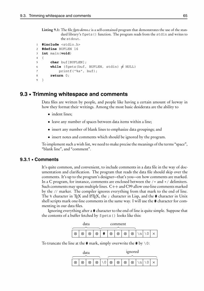
root2014/7/8page 65
�
�
�
�
�
�
�
�
9.3. Trimming whitespace and comments 65
Listing 9.1: The file fgets-demo.c is a self-contained program that demonstrates the use of the stan-dard library’s fgets() function. The program reads from the stdin and writes tothe stdout.
1 #include <stdio.h>2 #define BUFLEN 163 int main(void)4 {5 char buf[BUFLEN];6 while (fgets(buf, BUFLEN, stdin) �= NULL)7 printf("%s", buf);8 return 0;9 }
9.3 Trimming whitespace and commentsData files are written by people, and people like having a certain amount of leeway inhow they format their writings. Among the most basic desiderata are the ability to
• indent lines;
• leave any number of spaces between data items within a line;
• insert any number of blank lines to emphasize data groupings; and
• insert notes and comments which should be ignored by the program.
To implement such a wish list, we need to make precise the meanings of the terms “space”,“blank line”, and “comment”.
9.3.1 Comments
It’s quite common, and convenient, to include comments in a data file in the way of doc-umentation and clarification. The program that reads the data file should skip over thecomments. It’s up to the program’s designer—that’s you—on how comments are marked.In a C program, for instance, comments are enclosed between the /* and */ delimiters.Such comments may span multiple lines. C++ and C99 allow one-line comments markedby the // marker. The compiler ignores everything from that mark to the end of line.The % character in TEX and LATEX, the ; character in Lisp, and the # character in Unixshell scripts mark one-line comments in the same way. I will use the # character for com-menting in our data files.
Ignoring everything after a # character to the end of line is quite simple. Suppose thatthe contents of a buffer fetched by fgets() looks like this:
⊗ ⊗ ⊗ ⊗ # ⊗ ⊗ ⊗ ⊗ \n \0 ×data comment
To truncate the line at the # mark, simply overwrite the # by \0:
⊗ ⊗ ⊗ ⊗ \0 ⊗ ⊗ ⊗ ⊗ \n \0 ×data ignored

root2014/7/8page 66
�
�
�
�
�
�
�
�
66 Chapter 9. Reading lines: fetch_line()
Since the ASCII NUL character (\0) marks the end of a string, anything that comes afterit is immaterial.
9.3.2 Whitespace
When typing text into a text editor, you press the keyboard’s “space-bar” key to enterspaces between words; you may press the keyboard’s “Tab” key to indent the lines ofyour C program; you press the “Enter” key to insert a new line. These keys generate whatare known as whitespace characters. Words in a text document are typically separated bywhitespace.
There are other whitespace characters, although the common typewriter and com-puter keyboards don’t have dedicated keys for them. The C standard recognizes at leastsix whitespace characters (although it doesn’t call them “whitespace”): an ordinary space( ), form-feed (\f), newline (\n), carriage return (\r), horizontal tab (\t), and verticaltab (\v).27 It is important for our purposes to note that the ASCII NUL character (\0) isnot a whitespace character.
The C standard library provides the isspace() function which receives an objectas its argument and returns true if it is deemed whitespace, and false otherwise. The func-tion isspace() and a dozen or so other character-testing functions are declared in theheader file ctype.h; you need to #include it if you are going to use them. All those func-tions expect an unsigned char (or EOF) for their arguments; therefore the proper wayfor checking for a whitespace character requires a cast, as in
if (isspace((unsigned char)c))... do something ...
9.4 The programAs promised earlier, our fetch_line() reads the next available line from an inputstream, trims it of comments and leading and trailing whitespace, and returns a pointerto the trimmed string if the string is nonempty; otherwise it goes on to the next line andrepeats the process.
The file fetch-line.c contains the implementation of the function fetch_line().The header file fetch-line.h is the interface. The pair of files fetch-line.[ch] constitute ourfetch-line module. A third file, fetch-line-demo.c, contains a driver to demo that module.Thus, this project’s directory will contain
$ cd fetch-line$ ls -Ffetch-line-demo.c fetch-line.c fetch-line.h fgets-demo.c
The stand-alone test program fgets-demo.c was described in Section 9.2. The other threeprogram files are described below. We may automate the program’s compilation througha Makefile along the lines of the instructions in Chapter 6, but the current program is sosmall that writing a Makefile for it may be an overkill. To compile it manually, we do
$ gcc -c -Wall -pedantic -std=c89 -O2 fetch-line.c$ gcc -c -Wall -pedantic -std=c89 -O2 fetch-line-demo.c$ gcc fetch-line.o fetch-line-demo.o -o fetch-line-demo
27Additional characters may pass for whitespace depending on your locale environment. You will have toconsult the C standard if you want more details on this.

root2014/7/8page 67
�
�
�
�
�
�
�
�
9.5. The files fetch-line.[ch] 67
Listing 9.2: The header file fetch-line.h is fetch-line module’s interface.
1 #ifndef H_FETCH_LINE_H2 #define H_FETCH_LINE_H3 #include <stdio.h>4 char *fetch_line(char *buf, int buflen, FILE *stream, int *lineno);5 #endif /∗ H_FETCH_LINE_H */
You may change the std=c89 to std=c99 if you wish. The program is compatible withboth C89 and C99.
Here is a transcript of an interactive session with the program:
$ ./fetch-line-demo <fgets-demo.ctrimmed line 3: int main(void)trimmed line 4: {trimmed line 5: char buf[BUFLEN];
*** reading error: input line 6 too long for fetch_line’s buf[40]
As you see, we are feeding the file fgets-demo.c (which we encountered in Listing 9.1 onpage 65) to our demo program.28 Compare the program’s output shown here to the con-tents of fgets-demo.c. From fetch_line()’s point of view, the first two lines of the in-put are comments(!) since each begins with the # character; therefore they are discarded.The third line receives fetch_line()’s approval; hence it duly prints it, prefacing itwith the phrase “trimmed line 3:”. Line 4, consisting of a single { character, is alsoprinted without change. Line 5’s leading whitespace is trimmed away, and what remainsis printed. Line 6 is not acceptable to fetch_line(); it is too long to fit in a buffer oflength 40 which it is given to work with. Therefore it prints an error message and quits.If we increase the buffer size sufficiently (see the BUFLEN preprocessor macro in Part 9.1of Section 9.6), the program will read the file all the way to the end.
9.5 The files fetch-line.[ch]The files fetch-line.h and fetch-line.c contain our fetch-line module’s interface and imple-mentation, respectively. The contents of fetch-line.h are shown in their entirety in List-ing 9.2. That file’s sole purpose is to declare the prototype of the functionfetch_line()(on line 4). The standard library’s stdio.h header file is #included on line 3 to make theFILE symbol available for use in the next line. You will find an explanation of the #in-clude guards #ifndef ..., etc., on page 51.
The contents of the implementation file fetch-line.c are shown in an outline form inListing 9.3. It defines two functions, trim_line() and fetch_line(), whose pur-poses I will now describe.
9.5.1 The function trim_line()
The function trim_line() that appears on line 5 in Listing 9.3 is declared static29,indicating that it is only for internal use within the file fetch-line.c. The function’s sole ar-gument is a pointer s to a buffer which is expected to contain a properly NUL-terminatedstring. It trims the string of any leading or trailing whitespace and comments, as detailed
28You may feed any text file to the program; there is nothing special about fgets-demo.c, but it works nicelyfor demonstrating some of the features of our fetch-line module.
29See Section 1.6 regarding the static declaration specifier.
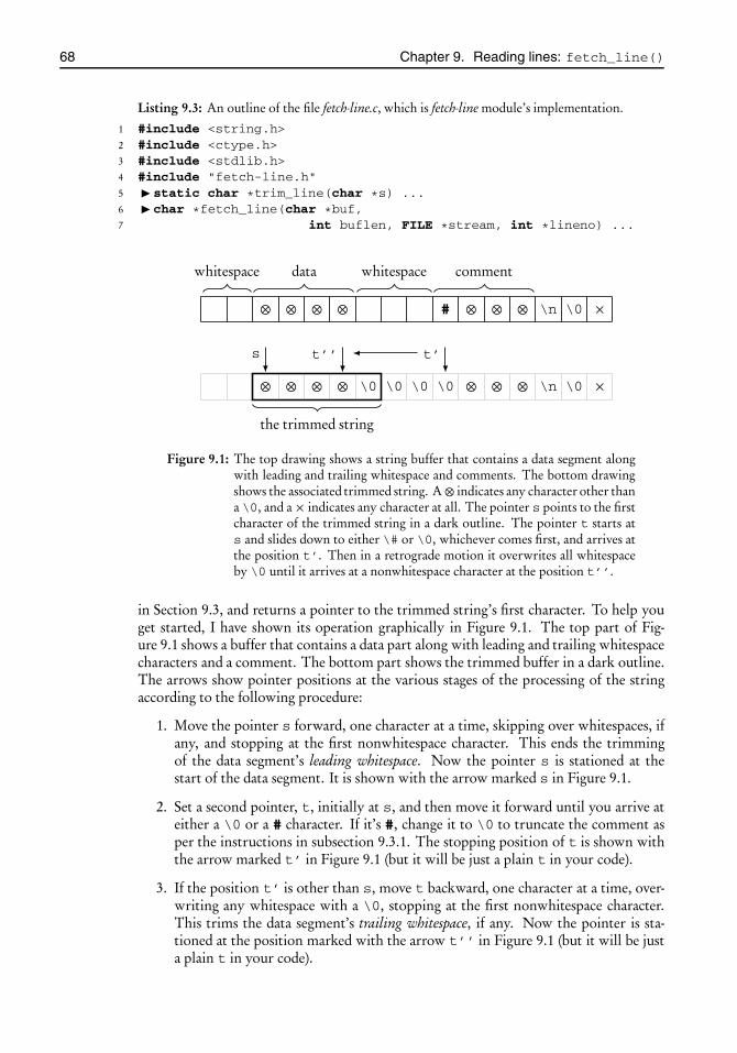
root2014/7/8page 68
�
�
�
�
�
�
�
�
68 Chapter 9. Reading lines: fetch_line()
Listing 9.3: An outline of the file fetch-line.c, which is fetch-line module’s implementation.
1 #include <string.h>2 #include <ctype.h>3 #include <stdlib.h>4 #include "fetch-line.h"5 � static char *trim_line(char *s) ...6 � char *fetch_line(char *buf,7 int buflen, FILE *stream, int *lineno) ...
⊗ ⊗ ⊗ ⊗ # ⊗ ⊗ ⊗ \n \0 ×whitespace data whitespace comment
⊗ ⊗ ⊗ ⊗ \0 \0 \0 \0 ⊗ ⊗ ⊗ \n \0 ×
the trimmed string
s t’t’’
Figure 9.1: The top drawing shows a string buffer that contains a data segment alongwith leading and trailing whitespace and comments. The bottom drawingshows the associated trimmed string. A⊗ indicates any character other thana \0, and a× indicates any character at all. The pointer s points to the firstcharacter of the trimmed string in a dark outline. The pointer t starts ats and slides down to either \# or \0, whichever comes first, and arrives atthe position t’. Then in a retrograde motion it overwrites all whitespaceby \0 until it arrives at a nonwhitespace character at the position t’’.
in Section 9.3, and returns a pointer to the trimmed string’s first character. To help youget started, I have shown its operation graphically in Figure 9.1. The top part of Fig-ure 9.1 shows a buffer that contains a data part along with leading and trailing whitespacecharacters and a comment. The bottom part shows the trimmed buffer in a dark outline.The arrows show pointer positions at the various stages of the processing of the stringaccording to the following procedure:
1. Move the pointer s forward, one character at a time, skipping over whitespaces, ifany, and stopping at the first nonwhitespace character. This ends the trimmingof the data segment’s leading whitespace. Now the pointer s is stationed at thestart of the data segment. It is shown with the arrow marked s in Figure 9.1.
2. Set a second pointer, t, initially at s, and then move it forward until you arrive ateither a \0 or a # character. If it’s #, change it to \0 to truncate the comment asper the instructions in subsection 9.3.1. The stopping position of t is shown withthe arrow marked t’ in Figure 9.1 (but it will be just a plain t in your code).
3. If the position t’ is other than s, move t backward, one character at a time, over-writing any whitespace with a \0, stopping at the first nonwhitespace character.This trims the data segment’s trailing whitespace, if any. Now the pointer is sta-tioned at the position marked with the arrow t’’ in Figure 9.1 (but it will be justa plain t in your code).

root2014/7/8page 69
�
�
�
�
�
�
�
�
9.5. The files fetch-line.[ch] 69
Listing 9.4: The function fetch_line() reads and returns the next nonempty trimmed linefrom the input stream. If the input line is too long to fit in the given buffer, it prints adiagnostic and calls exit().
1 char *fetch_line(char *buf, int buflen, FILE *stream, int *lineno)2 {3 char *s;4 if (fgets(buf, buflen, stream) == NULL)5 return NULL;6 ++*lineno;7 if (buf[strlen(buf) - 1] �= ’\n’) {8 fprintf(stderr, "*** reading error: input line %d too "9 "long for %s’s buf[%d]\n",
10 *lineno, __func__, buflen);11 exit(EXIT_FAILURE);12 }13 s = trim_line(buf);14 if (*s �= ’\0’)15 return s;16 else17 return fetch_line(buf, buflen, stream, lineno); // recurse18 }
At the completion of the process, the pointer s points to the trimmed data string. Thefunction trim_line() returns that pointer to the caller. You have all the necessaryinformation now to implement your own trim_line().
Remark 9.2. If a string contains nothing but comments and whitespace, then itis reduced to an empty string after trimming. Consequently, the pointer returned bytrim_line() points to \0. We use this observation in the next subsection to skip overempty lines in an input stream.
9.5.2 The function fetch_line()
The function fetch_line() that appears on line 6 in Listing 9.3 is presented in itsentirety in Listing 9.4. The caller of fetch_line() supplies the buffer buf of lengthbuflen and a stream which is open for reading. fetch_line() calls fgets() toread a line from stream into buf and then passes that line to trim_line() to stripit of comments and leading and trailing whitespace. If the trimmed string is nonempty,then fetch_line() returns a pointer to the start of that string; otherwise it calls itselfrecursively in search of a nonempty line. If the end of the input is reached, or if the callto fgets() experiences an error, fetch_line() returns NULL.
Our fetch_line() is not designed to resize the buffer. If an input line is too long tofit, fetch_line() takes a very drastic action: it prints a diagnostic message to stderrand then calls exit() to abort the program! There are other ways of handling suchcontingencies; I have chosen this extremely drastic route because it’s the only useful actionfor our purposes.
How does fetch_line() tell if a line is too long to fit? Since the lines are readby fgets(), and since fgets() includes the line’s terminating newline character inthe fetched buffer, as shown in the “case 3” figure on page 64, then a properly fitting linewill be a string terminated by the two characters \n\0; that is, the string’s last character,

root2014/7/8page 70
�
�
�
�
�
�
�
�
70 Chapter 9. Reading lines: fetch_line()
Listing 9.5: The file fetch-line-demo.c is a driver for the fetch-line module.
1 #include <stdio.h>2 #include "fetch-line.h"3 #define BUFLEN 404 int main(void)5 {6 char buf[BUFLEN];7 char *s;8 int lineno = 0;9 while ((s = fetch_line(buf, BUFLEN, stdin, &lineno)) �= NULL)
10 printf("trimmed line %3d: %s\n", lineno, s);11 return 0;12 }
just before the null terminator, will be \n. In Listing 9.4 we determine a string’s lastcharacter with the help of the standard library’s strlen() function, which returns astring’s length.
fetch_line()’s fourth argument, lineno, is a pointer to an integer that holds thevalue of the current line number. Whenever fetch_line() reads a line, it incrementsthe number stored there. The caller may refer to that number when issuing diagnosticsabout possible errors in the input.
9.6 Project fetch_line
Part 9.1. Listing 9.5 shows a minimalistic driver to demonstrate the functionality of ourfetch-line module. It sets up a buffer of length BUFLEN and then calls fetch_line() ina loop to read lines from the program’s stdin into that buffer. It also sets up an integercounter, lineno, initialized to zero, whose address is passed to fetch_line(). As wesaw in subsection 9.5.2, fetch_line() increments that counter every time it reads aline. Therefore lineno will contain the line number of the current line at any time. Theprogram writes out that information to the stdout in Listing 9.5, line 10.
Encode, compile, and test your fetch_line program. See the sample session onpage 67.
Part 9.2. Suppose BUFLEN is 40, as before. Create a file with gradually increasing linelengths, e.g.,
35xxxxxxxxxxxxxxxxxxxxxxxxxxxxxxxxx36xxxxxxxxxxxxxxxxxxxxxxxxxxxxxxxxxx37xxxxxxxxxxxxxxxxxxxxxxxxxxxxxxxxxxx... more lines here ...42xxxxxxxxxxxxxxxxxxxxxxxxxxxxxxxxxxxxxxxx
where the number at the beginning of each line equals the total length of that line. Whathappens when you feed that file to your program? Explain what you observe.
Part 9.3. Add whitespace (spaces, tabs, empty lines) and comments in various places inthe file that you created in Part 9.2. Verify that your program behaves as intended.
root2014/7/8page 71
�
�
�
�
�
�
�
�
Chapter 10
Generating randomnumbers
Prerequisites: Chapters 7, 8
10.1 The rand() and srand() functionsThe C standard library provides a pseudorandom number generator through the rand()function. Together with the associatedsrand() function, they are declared instdlib.has “int rand(void);” and “void srand(unsigned int seed);”.
Each call to rand() returns a random integer n with a uniform probability distribu-tion in the range 0 ≤ n ≤ RAND_MAX. The value of RAND_MAX, a large positive integer,is built into your C library and cannot be changed. The C library on my computer hasRAND_MAX = 231 − 1 = 2,147,483,647. It may be something else on yours.30 Here is acomplete program that prints four random numbers:
#include <stdio.h>#include <stdlib.h>int main(void){
for (int i = 0; i < 4; i++)printf("%d ", rand());
putchar(’\n’);return 0;
}
Here is what it prints:
1804289383 846930886 1681692777 1714636915.
If you run the program once again, it will print exactly the same four numbers! This isnot a bug—even a statistician likes reproducible experiments!
Nevertheless, if you truly want your program to generate a different sequence of ran-dom numbers, invoke srand(n) with some positive integer n—called the random gen-erator’s seed—to alter the random generator’s initial state, as in
#include <stdio.h>#include <stdlib.h>
30You can find out the value of RAND_MAX on your machine by printing it in a C program, as inprintf("RAND_MAX = %u\n", RAND_MAX); Alternatively, you may just look it up in stdlib.h if youknow where to find that header file. On a typical Unix installation it is /usr/include/stdlib.h.
71

root2014/7/8page 72
�
�
�
�
�
�
�
�
72 Chapter 10. Generating random numbers
int main(void){
srand(7); // set seed to 7for (int i = 0; i < 4; i++)
printf("%d ", rand());putchar(’\n’);return 0;
}
Now the program prints
1045618677 1863967299 1272579899 461085871.
Setting the seed to 1 is equivalent to not calling srand() at all.To generate random fractional numbers r in the closed interval [0,1], divide the value
returned by rand() by RAND_MAX, as in r = (double)rand()/RAND_MAX. Thecast is necessary; otherwise the quotient is zero according to C’s integer division rules.To generate random fractional numbers R in a prescribed interval [a, b ], generate themin [0,1] as above and then map them to [a, b ] through scaling, as in R= a+(b − a)r .
Producing random integers on a prescribed integer range is a more challenging prob-lem. To simulate a coin tossing experiment, for instance, we want random numbers in theset {0,1}. To simulate the tossing of dice, we want random numbers in the set {1,2, . . . , 6}.Unfortunately there is no simple and perfect way of doing this. A reasonably good way ofgenerating uniformly distributed random integers r in the set {0,1, . . . , n− 1} is throughthe formula
r=rand()
RAND_MAX
n+ 1
(n RAND_MAX),
where both divisions are performed in the sense of integer arithmetic; that is, the quotientis computed and the remainder is discarded. (C’s integer arithmetic does that by default.)The formula works well when n is much smaller than RAND_MAX.31 To dramatize thatstatement, let us say RAND_MAX is 1,000. (This is far from realistic; on a typical imple-mentation, RAND_MAX will be millions of times larger.) If n = 6, as in a die throwingexperiment, then the likelihood of obtaining a 0 (or a 1, or 2, or 3, or 4) according to thatformula is 167/1001, but the likelihood of obtaining a 5 is 166/1001, which is just slightlylower but not too bad. On the other hand, if n = 30, then the likelihood of obtaininga 0 (or a 1, or . . . 28) is 34/1001, but the likelihood of obtaining a 29 is 15/1001, which issignificantly lower.
In the applications of interest to us, the values of n are millions of times smaller thanRAND_MAX; therefore we run no risk of skewing our statistics by using that formula. Infact, we package the formula in a convenient function, which we call random(), forfuture use. Listing 10.1 shows the essentially one-line implementation.
Remark 10.1. The inline specifier in the function’s declaration makes it an inline func-tion, which has the effect of suggesting to the compiler that the calls to this function are tobe as fast as possible. The C standard does not prescribe how that is to be accomplished.The compiler may, at its discretion, dismantle the function and conceptually embed itsbody where it’s called, thus obviating the overhead of a function call altogether. Or it
31I learned about this formula from <http://www.c-faq.com/lib/randrange.html>. That pagealso offers a method, at the cost of some loss of efficiency, for dealing with situations where n is not necessarilysmall compared to RAND_MAX.

root2014/7/8page 73
�
�
�
�
�
�
�
�
10.2. Bitmap images 73
Listing 10.1: Returns a random integer in the set {0,1, . . . , n − 1} with uniform distribution. As-sumes n is much smaller than RAND_MAX.
1 inline int random(int n)2 {3 return rand()/(RAND_MAX/n + 1);4 }
may take some other measures to speed up the function’s use. Or it may just ignore theinlining request altogether.
The inline specifier was introduced in C99. If your compiler does not support it,it’s safe to remove it.
Remark 10.2. The C standard does not prescribe an algorithm for the pseudoran-dom number generator (PRNG) associated with rand(). Its only requirement is thatRAND_MAX be at least 32767. The algorithm is left up to the implementation.
Earlier implementations of the standard library’s rand() developed a (well-deserved)reputation for being too naive; the data they generated could hardly pass even the sim-plest tests for randomness. Serious users shunned the standard library’s rand() andused PRNGs of their own, or something else made by third parties. Some computer plat-forms supplied their own (nonstandard) PRNG, usually called random(), as an alter-native to the standard rand(). Things have improved over the years. The rand()and random() functions that comes with modern Linux distributions, for instance,both use the same rather sophisticated algorithm, which has a period of approximately16× (231 − 1). To learn more about PRNGs, consult Numerical Recipes in C [53], whichdevotes an entire chapter to the subject.
Remark 10.3. The name “random” used for the function defined in Listing 10.1 is quitelegitimate within standard C. It is likely, however, that your computer platform suppliesa nonstandard PRNG called random(), as noted in the previous paragraph. So, which ofthe two random() functions will your program use?
To avoid a potential clash between the two, be sure to tell your compiler to treat yourprogram as strictly standard C. For example, if you use the GNU C compiler, invokeit with the -std=c89 or the -std=c99 flag. In the worst case, if you have a brokencompiler that refuses to understand about standards, then rename the random() in List-ing 10.1 to Random(), or somesuch.
10.2 Bitmap imagesWe intend to exercise our random() function of Listing 10.1 to produce bitmap imageslike those shown in Figure 10.1. A bitmap image is a rectangular array of black and whitedots.
It is natural to represent a bitmap image as a matrix of zeros and ones. Each of thematrix’s entries corresponds to a dot in the image. A zero represents a white dot, a 1 ablack dot. The Portable Bitmap (PBM) convention for storing bitmap images formalizesthis idea: You put the matrix of zeros and ones in a file, say sample-bitmap.pbm, and adda header consisting of the two-character magic number32 P1, along with the image’s widthand the height (in that order). Then you may view the image by passing the file name
32See footnote 43 on page 115 for the meaning of the “magic number”.

root2014/7/8page 74
�
�
�
�
�
�
�
�
74 Chapter 10. Generating random numbers
(a) (b) (c)
Figure 10.1: Three 100× 200 bitmap images of random noise. From left to right, thefill ratio is 0.10, 0.20, and 0.40.
P14 71 1 1 11 0 0 01 0 0 01 1 1 01 0 0 01 0 0 01 0 0 0
Figure 10.2: On the left are the contents of a PBM definition file. On the right is thecorresponding 7×4 bitmap image. I have superimposed a grid to delineatethe pixels. Beware that the image shown is greatly magnified; a 7×4 bitmapimage in its natural size is too small for viewing on a computer screen, butyou can ask your image viewer to magnify it.
sample-bitmap.pbm to almost any image viewer. Figure 10.2 shows the contents of a PBMfile and the corresponding image.
Remark 10.4. As simple as it is, the plain PBM format which I have described here isthe most wasteful way of storing a bitmap image. Much better ways are available. SeeChapter 14 for further discussion of bitmaps and other forms of representing images.
10.3 The programIn principle, one can encapsulate the random() function of Listing 10.1 in a moduleconsisting of a pair of files random.h and random.c. I will not take that route, however,since the function is so simple—a one-liner, actually—that the ado about an interface andan implementation will blow things way out of proportion. I would rather just insert acopy of the four lines of Listing 10.1 into a program, wherever it’s needed. I will take thatapproach in this chapter and elsewhere.
Here is this chapter’s project. Take an m × n matrix, and imagine that its entriesrepresent a rectangular array of m rows and n columns of white dots. Then begin selectingrandom dots and coloring them black. Repeat until a certain percentage, say 10%, of thedots have been colored. That will produce a picture like Figure 10.1(a). We say that thefill ratio of that picture is 0.10. The pictures (b) and (c) have fill ratios of 0.20 and 0.40,respectively.
Figure 10.1(a) was produced by executing the command
$ ./random-pbm 100 200 1 0.10 rand-10.pbm
Those command-line arguments request a 100× 200 image and set the random numbergenerator’s seed to 1, the fill ratio to 0.10, and the name of the output file (that is, the image

root2014/7/8page 75
�
�
�
�
�
�
�
�
10.4. The file random-pbm.c 75
Listing 10.2: An outline of the file random-pbm.c.
1 #include <stdio.h>2 #include <stdlib.h>3 #include "array.h"4 � static inline int random(int n) ...5 � static int write_pbm(char **M, int m, int n, char *outfile) ...6 � static char **make_random_matrix(int m, int n, double f) ...7 � static void show_usage(char *progname) ...8 � int main(int argc, char **argv) ...
file) to rand-10.pbm. If the program is invoked with insufficient or illegal command-linearguments, it prints a help message to the stderr and exits, as in
$ ./random-pbmUsage: ./random-pbm m n s f outfile
writes an mxn random bitmap to a file named ‘outfile’f: fill ratio 0.0 <= f <= 1.0s: integer >= 1: seeds the random number generator
We use Chapter 7’s Xmalloc module and Chapter 8’s array.h header file to allocatememory for the bitmap’s matrix. Therefore, following the suggestions of Chapters 2and 6, the program’s directory will look like this:
$ cd random$ ls -FMakefile array.h@ random-pbm.c xmalloc.c@ xmalloc.h@
I will describe the contents of the file random-pbm.c in the next section.
10.4 The file random-pbm.cListing 10.2 gives an outline of the file random-pbm.c. The function random() that ap-pears on line 4 is the same as that shown in Listing 10.1. The function show_usage()that appears on line 7 is responsible for printing the help message shown in Section 10.3.I will let you write it. The remaining three functions are described in the following sub-sections.
10.4.1 The function main()
The function main() that appears on line 8 of Listing 10.2 is responsible for parsing thecommand-line arguments and then directing the rest of the program’s flow. The initialpart of the function main() is shown in Listing 10.3. Let me explain some of the details.
Line 5. The matrix M will hold the bitmap’s data. Since the data consists of zeros andones, any integer data type will do. We choose char here since it is the smallestsuch data type.
Line 8. The variable status holds the program’s exit status. We initialize it to the de-fault of EXIT_FAILURE. Later on, after obtaining reassurance that the programhas succeeded (line 38 in Listing 10.4), we will change it to EXIT_SUCCESS.
Line 9. As we saw in Section 10.3, the program is expected to be invoked with five ar-guments, and therefore argc should be 6; see Section 4.7 regarding command-line

root2014/7/8page 76
�
�
�
�
�
�
�
�
76 Chapter 10. Generating random numbers
Listing 10.3: The initial part of the function main() in file random-pbm.c.
1 int main(int argc, char **argv)2 {3 int m, n, s; // image is m× n, seed is s4 double f; // fill ratio5 char **M;6 char *outfile;7 char *endptr;8 int status = EXIT_FAILURE;9 if (argc �= 6) {
10 show_usage(argv[0]);11 return EXIT_FAILURE;12 }13 m = strtol(argv[1], &endptr, 10);14 if (*endptr �= ’\0’ || m < 1) {15 show_usage(argv[0]);16 return status;17 }18 // · · · similarly, extract n, s, f, and outfile
arguments. If argc is not 6, we print a usage message and exit. We pass argv[0]toshow_usage() so that it can print the program’s name along with the message.See the sample message shown in Section 10.3.
Line 13. We call the standard library’s strtol() function (Chapter 5) to translate thestring argv[1] to an integer. Subsequently, we verify that argv[1] is a properrepresentation of an integer and that its numerical value is no less than 1. If not, weprint a usage message and exit.
Lines 18–34. Here I have excised several lines from main() to give you an opportunityto insert your own code. You will need to extract the integers n and s, the floatingpoint number f, and the string outfile from the command-line arguments. Youwill use the strtod() function (Chapter 5) to extract the value of f.
The remaining part of the function main() is shown in Listing 10.4. Let us examine thedetails.
Line 35. Now that we have extracted the user-specified value of the seed s for the randomnumber generator, we call srand() to set the seed to s.
Line 36. We call the function make_random_matrix() (to be described later) to pro-duce an m× n matrix of random zeros and ones with a fill ratio of f .
Line 37. We call the function write_pbm() (to be described later) to write the matrix’sdata as a PBM file. The function returns 1 on success and 0 on failure. (The mostlikely cause of failure is the lack of permission to open the file for writing.) If thecall returns 1, then it has succeeded; therefore we change the value of status toEXIT_SUCCESS.
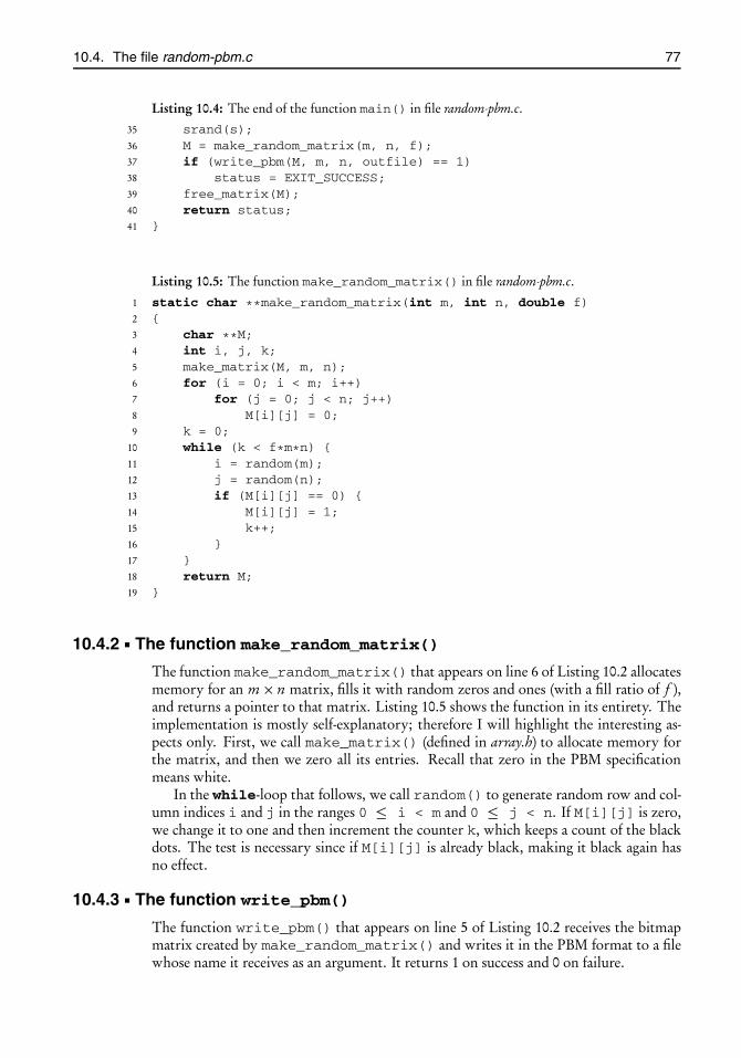
root2014/7/8page 77
�
�
�
�
�
�
�
�
10.4. The file random-pbm.c 77
Listing 10.4: The end of the function main() in file random-pbm.c.
35 srand(s);36 M = make_random_matrix(m, n, f);37 if (write_pbm(M, m, n, outfile) == 1)38 status = EXIT_SUCCESS;39 free_matrix(M);40 return status;41 }
Listing 10.5: The function make_random_matrix() in file random-pbm.c.
1 static char **make_random_matrix(int m, int n, double f)2 {3 char **M;4 int i, j, k;5 make_matrix(M, m, n);6 for (i = 0; i < m; i++)7 for (j = 0; j < n; j++)8 M[i][j] = 0;9 k = 0;
10 while (k < f*m*n) {11 i = random(m);12 j = random(n);13 if (M[i][j] == 0) {14 M[i][j] = 1;15 k++;16 }17 }18 return M;19 }
10.4.2 The function make_random_matrix()
The function make_random_matrix() that appears on line 6 of Listing 10.2 allocatesmemory for an m× n matrix, fills it with random zeros and ones (with a fill ratio of f ),and returns a pointer to that matrix. Listing 10.5 shows the function in its entirety. Theimplementation is mostly self-explanatory; therefore I will highlight the interesting as-pects only. First, we call make_matrix() (defined in array.h) to allocate memory forthe matrix, and then we zero all its entries. Recall that zero in the PBM specificationmeans white.
In the while-loop that follows, we call random() to generate random row and col-umn indices i and j in the ranges 0 ≤ i < m and 0 ≤ j < n. If M[i][j] is zero,we change it to one and then increment the counter k, which keeps a count of the blackdots. The test is necessary since if M[i][j] is already black, making it black again hasno effect.
10.4.3 The function write_pbm()
The function write_pbm() that appears on line 5 of Listing 10.2 receives the bitmapmatrix created by make_random_matrix() and writes it in the PBM format to a filewhose name it receives as an argument. It returns 1 on success and 0 on failure.

root2014/7/8page 78
�
�
�
�
�
�
�
�
78 Chapter 10. Generating random numbers
I will describe the function’s overall plan in words and let you fill in the details. First,call the standard library’s fopen() to open the output file for writing. If unsuccessful,print an appropriate message to the stderr, and then return 0. Next, write the image’sheader as described in Section 10.2. See Figure 10.2 for a sample. Then write the data partaccording to the contents of the matrix M. Finally, close the output stream and return 1.You may use the print_matrix() macro from Part 8.3 of Project array.h (page 60) toprint the matrix M.
10.5 Project Random BitmapsComplete the file random-pbm.c according to the given instructions, and then compileand experiment. Width and height values in the range 100 to 400 produce bitmaps ofreasonable size for viewing on a computer screen.
There are very many utilities for viewing images. The choice depends in your platformand personal preference. I do all of my work on a Linux laptop. Mostly I use feh forviewing images. Occasionally I use thedisplay utility that comes with the ImageMagickpackage and the venerable xv, which, unfortunately, is no longer actively maintained.
root2014/7/8page 79
�
�
�
�
�
�
�
�
Chapter 11
Storing sparse matrices
Prerequisites: Chapters 7, 8
11.1 IntroductionA sparse matrix is a matrix whose entries are mostly zero. Large sparse matrices occurquite frequently in computing. In solving a linear Partial Differential Equation (PDE)with the Finite Element Method (FEM), for instance, one subdivides the equation’s do-main into a fine mesh of simple objects such as triangles or tetrahedra and approximatesthe PDE’s solution with low degree polynomials in each. This reduces the task of solv-ing the PDE to solving a linear system of equations Ax = b , where the n× n coefficientmatrix A tends to be quite large; n = 10,000 is not out of the ordinary. Storing such ahumongous matrix can pose challenges for the computer’s memory and disk utilization.Fortunately, it is hardly ever necessary to store the matrix in toto since by the nature ofthe FEM, all but a tiny fraction of the matrix’s entries are zeros in general.
Depending on the FEM’s algorithm, the total number of nonzero entries in the n×nmatrix A may be as little as 3n. When n = 10,000, for instance, such a matrix will have atotal of 100,000,000 entries, only 30,000 of which are nonzero. In other words, only oneout of 3,333 entries is nonzero! So it would make sense to store only the nonzero entriesalong with their indices into A, rather than a hundred million zeros.
There is no standard way of storing sparse matrices—see [18, Chapter 2] and [6, Sec-tion 4.3] for surveys of the various methods—although the Compressed Column Storage(CCS) format appears to be the favorite choice nowadays, perhaps because that’s whatMATLAB uses.
It is this chapter’s objective to introduce the CCS format and see how it translatesto C code. The functions sparse_pack() and sparse_unpack() developed in theprocess convert a matrix to and from the CCS format. I must point out that we haveno practical use for these functions in the rest of the book since our work with sparsematrices will be handled through the facilities provided by the UMFPACK library, whichis the subject of the next chapter. Interacting with UMFPACK, however, does require someunderstanding of the CCS format, and that’s what you are expected to take with you fromthis chapter.
79

root2014/7/8page 80
�
�
�
�
�
�
�
�
80 Chapter 11. Storing sparse matrices
11.2 The CCS formatI will explain the CCS format in terms of the concrete 4× 5 matrix
A=
⎛⎜⎜⎝0 7 0 0 10 4 0 3 06 6 5 1 45 5 0 0 0
⎞⎟⎟⎠ ,
which is neither large nor truly sparse; nevertheless, it will serve quite adequately forconveying the idea behind CCS.
The matrix has 11 nonzero entries. Following [16] and [18], I will write nz for thenumber of a matrix’s nonzero entries. The obvious—but not the best—way of storing thematrix’s nonzero entries is as a set of nz triplets (i , j ,Ai j ) of locations and values. Weput the first components of such triplets into a vector Ai, the second components into avector Aj, and the third components into a vector Ax, and thus we get three vectors oflength nz each:
Ai= [ 2 3 0 1 2 3 2 1 2 0 2 ],Aj= [ 0 0 1 1 1 1 2 3 3 4 4 ],Ax= [ 6 5 7 4 6 5 5 3 1 1 4 ].
(Note that we are counting the row and column indices beginning with zero.) To producethis list, I scanned the matrix by columns from top to bottom and then from left to right.That’s where the “column” in the CCS comes in.33 There is a “Fortran accent” in thissince that’s the order in which matrix entries are stored in Fortran. (In contrast, C’sbuilt-in array types store two-dimensional arrays in the row order.) The CCS format wasdeveloped when Fortran was—some say it still is—the dominant programming languagein scientific computing.
As I noted above, the storage of A as the three vector set { Ai, Aj, Ax } is not the bestwe can do. A hint to the suboptimality of that representation is provided by the repetitivenature of the entries of the Aj vector. Have a look. The first two “0”s in Aj tell us thatthe matrix A has two nonzero entries in its first column. The next four “1”s in Aj tell usthat A has four nonzero entries in its second column, and so on. Can’t we express thatinformation in a more concise way? Yes, we can! For instance, the vector
A’= [ 2 4 1 2 2 ]
conveys exactly the same information as Aj (two entries in the first column, four entriesin the second column, etc.) and it is shorter.
The CCS format is a slight variant of this idea. For an m× n matrix A it introducesa vector Ap of length n + 1 with the property that Ap[j] gives the index in the vectorAx of where the matrix’s column j begins. More precisely, the vector Ap is such that theentries in the matrix’s jth column are given by
{ Ax[k] : Ap[j] ≤ k < Ap[j+1] }.34 (11.1)
33It should be obvious that the order in which the matrix’s entries are scanned is immaterial for the purposeof its representation as the { Ai, Aj, Ax } three-vector set. But the order does matter where the vector Ap isintroduced later on.
34This implies, in particular, that Ap[n] = nz.
root2014/7/8page 81
�
�
�
�
�
�
�
�
11.4. The files sparse.[ch] 81
For our matrix A we have Ap= [ 0 2 6 7 9 11 ] becausethe values { Ax[k] : 0 ≤ k < 2 } go to the matrix’s first column,the values { Ax[k] : 2 ≤ k < 6 } go to the matrix’s second column,the values { Ax[k] : 6 ≤ k < 7 } go to the matrix’s third column,the values { Ax[k] : 7 ≤ k < 9 } go to the matrix’s fourth column,the values { Ax[k] : 9 ≤ k < 11 } go to the matrix’s fifth column.
To conclude, the matrix A and its CCS representation are
A=
⎛⎜⎜⎝0 7 0 0 10 4 0 3 06 6 5 1 45 5 0 0 0
⎞⎟⎟⎠ ⇐⇒⎧⎪⎨⎪⎩
Ap= [ 0 2 6 7 9 11 ],Ai= [ 2 3 0 1 2 3 2 1 2 0 2 ],Ax= [ 6 5 7 4 6 5 5 3 1 1 4 ].
The sparse matrix representation is not particularly useful in this instance since it wouldhave been more economical to store the matrix’s 4× 5= 20 entries, zeros and all, insteadof the 6+ 11+ 11 = 28 numbers that make up the vectors Ap, Ai, Ax. The benefits ofsparse storage become apparent only when the matrix is large and has a small fraction ofnonzero entries.
11.3 The programWe are going to write a sparse matrix module in a file sparse.c that contains two C func-tions, sparse_pack() and sparse_unpack(). The first receives an m× n matrixand computes the corresponding CCS vectors Ap, Ai, Ax. The second does the reverse;that is, it receives the CCS vectors Ap, Ai, Ax and constructs the matrix A. Additionally,we will write a test/demo program in sparse-test.c to exercise those functions. The pro-gram depends on array.h (Chapter 8) and xmalloc.[ch] (Chapter 7) for allocating memoryfor vectors and matrices; therefore, following the suggestions of Chapters 2 and 6, yourproject’s directory will look like this:
$ cd sparse$ ls -FMakefile array.h@ sparse.c sparse.h xmalloc.c@ xmalloc.h@
Our implementations of sparse_pack() and sparse_unpack()work with ma-trices of type double. These are the types of matrices that most frequently require sparsestorage. Should you have a need to work with matrices of a different type, you will haveto write another pair of functions for that type. It is possible to apply Chapter 8’s pre-processor trick to produce type-generic versions of these, but it’s probably not worth theeffort since the need for sparse storage of matrices other than the type double is so rare.
11.4 The files sparse.[ch]The functions sparse_pack() and sparse_unpack(), defined in the file sparse.c,deal with preallocated vectors and matrices. That is, the caller is expected to have allocatedproperly sized vectors and matrices before calling these function. They do no memoryallocations on their own.
The implementation of the function sparse_pack() is quite straightforward, so Iwill leave it to you to write. The function sparse_unpack(), which is only slightlymore involved, is shown in Listing 11.1. It receives the CCS vectors Ap, Ai, Ax andpopulates the m× n matrix A with them.

root2014/7/8page 82
�
�
�
�
�
�
�
�
82 Chapter 11. Storing sparse matrices
Listing 11.1: The implementation of the function sparse_unpack(). It receives the CCS vec-tors Ap, Ai, Ax and populates the m× n matrix A with them.
1 void sparse_unpack(double **a, int m, int n,2 int *Ap, int *Ai, double *Ax)3 {4 int i, j, k;5 for (i = 0; i < m; i++)6 for (j = 0; j < n; j++)7 a[i][j] = 0.0;8
9 for (j = 0; j < n; j++)10 for (k = Ap[j]; k < Ap[j+1]; k++) {11 i = Ai[k];12 a[i][j] = Ax[k];13 }14
15 }
The function begins with storing zeros for all entries in the matrix A. After all, A issupposedly sparse; therefore most of its entries are zeros anyway. The nested for-loopthat begins on line 9 decodes the CCS vectors. The outer for-loop steps through thecolumns 0 ≤ j < n. The inner for-loop extracts that column’s entries according to theformula (11.1) on page 80 and inserts them into the matrix A.
To complete the module, write a header file, sparse.h, that provides the module’s in-terface. Don’t forget to put #include guards in sparse.h and #include"sparse.h" insparse.c.
11.5 Project Sparse MatrixComplete the files sparse.c and sparse.h, as instructed in the previous sections. Then writefile sparse-test.c, which provides a test/demo of our sparse module. I will describe its con-tents in words and let you make it into a C program.
• Create the 4× 5 matrix A of Section 11.2. Thus, let m = 4, n = 5, and then
double **a;make_matrix(a, m, n);a[0][0] = 0; a[0][1] = 7; ...
• Step through the matrix and count the number of its nonzero entries. Call it nz.
• Print the matrix and nz.
• Callmake_vector() to make the CCS vectors Ap, Ai, Ax of appropriate lengths.
• Call sparse_pack() to encode the matrix into the CCS vectors.
• Print the vectors Ap, Ai, Ax.
• Make an m × n matrix b. Call sparse_unpack() to unpack the CCS vectorsinto the matrix b.
root2014/7/8page 83
�
�
�
�
�
�
�
�
11.5. Project Sparse Matrix 83
• If your code is working properly, the matrices a and b should be identical; thereforetheir difference should be zero. To verify this, make a third m × n matrix; let’scall it c. In a doubly nested for-loop, set c[i][j] = a[i][j] - b[i][j].Print the matrix c. Is it all zeros?
• Free all allocated memory before exiting.
For your reference, here is what my program prints:
The sparse matrix is0 7 0 0 10 4 0 3 06 6 5 1 45 5 0 0 0
matrix is 4x5, nz = 11
Ap = 0 2 6 7 9 11Ai = 2 3 0 1 2 3 2 1 2 0 2Ax = 6 5 7 4 6 5 5 3 1 1 4
The difference of the original and reconstructed matrices:0 0 0 0 00 0 0 0 00 0 0 0 00 0 0 0 0
As you see, there are quite a few calls to print vectors and matrices. You may put thetype-generic print_vector() and print_matrix() macros developed in Part 8.3of Project array.h (page 60) to good use here.
root2014/7/8page 85
�
�
�
�
�
�
�
�
Chapter 12
Sparse systems:The UMFPACK library
Prerequisites: Chapters 7, 8, 11
12.1 IntroductionUMFPACK (pronounced in two syllables: “umph”–“pack”) is a library of C functions forsolving systems of linear equations Ax = b , where A is an n × n matrix and b is ann-vector. Although it will work with any nonsingular A, it is particularly effective in thesituations where A is large and sparse. The library, written by Tim Davis, is available asan open and free software from
<http://www.cise.ufl.edu/research/sparse/umfpack/>.It incorporates state-of-the-art algorithms for solving large sparse systems developed byDavis and a host of collaborators, and underlies many computational algorithms in soft-ware packages such as Comsol, Maple, and MATLAB.
This chapter introduces some of the most basic aspects of the UMFPACK library andshows how to interface with it in a C program. We cover only what is needed in appli-cations to finite elements in Chapters 25 and 26. To learn more, you should read UMF-PACK’s Quick Start Guide and User Guide (17 pages and 133 pages, respectively, as ofVersion 5.4.0, dated May 20, 2009) that come with UMFPACK as PDF files. Additionally,you may benefit from reading Davis’s book [16] and the articles [14, 15].
12.2 The basicsUMFPACK expects the n × n coefficient matrix A of the system Ax = b to be given inthe CCS format, that is, as the three vectors Ap, Ai, and Ax, as seen in Chapter 11. Thevector Ap is of length n+1, while Ai and Ax are of length nz each, where nz is the countof A’s nonzero entries. The system’s right-hand side, b , is an ordinary vector of length n.Solving the system Ax = b proceeds in three stages:
Stage 1: Symbolic analysis. We pass the matrix A (actually, the CCS vectors Ap, Ai, andAx) to the UMFPACK function umfpack_di_symbolic() for symbolic analysis.The goal of this stage is to analyze the pattern of distribution of the nonzero entriesin the sparse matrix A; their numeric values are immaterial. UMFPACK applies aseries of row and column permutations to arrange the pattern of the nonzeros in acertain optimal way. This transforms the matrix A to a matrix PAQ, where P and Qare permutation matrices.
85
root2014/7/8page 86
�
�
�
�
�
�
�
�
86 Chapter 12. Sparse systems: The UMFPACK library
Remark 12.1. A permutation matrix is the result of shuffling the rows or columnsof the n× n identity matrix. If the permutation matrix P is produced by shufflingthe rows of the identity matrix, then the left-multiplication PA with an arbitraryn × n matrix A applies exactly those row shuffles to A. If the permutation ma-trix P is produced by shuffling the columns of the identity matrix, then the right-multiplication AP with an arbitrary n × n matrix A applies exactly those columnshuffles to A. A permutation matrix is an orthogonal matrix, that is, P T P = I ,where I is the identity matrix and P T is the transpose of P .
Stage 2: Numeric analysis. We pass the matrix A and the permutation data (effectivelythe P and Q permutations matrices from the previous step) to the UMFPACK func-tion umfpack_di_numeric(), which applies Gaussian elimination to performan LU factorization of the permuted matrix; that is, it computes L and U so thatPAQ = LU , where L and U are n × n matrices, L is lower-triangular, and U isupper-triangular.
Stage 3: Solving the system. We pass the matrix A, the LU factorization data from theprevious step, the vector b , and the address of a preallocated vector x to the UMF-PACK function umfpack_di_solve(), which solves the system Ax = b andplaces the solution in the vector x.
Let me explain that last step in a little more detail. From the LU factorization PAQ =LU and the orthogonality of P and Q it follows that A= P T LU QT ; therefore the systemAx = b takes the form P T LU QT x = b , or equivalently, LU QT x = P b . Introducing thetemporary variable y = U QT x reduces the equation to the linear system Ly = P b , whichis quite trivial to solve for y since the coefficient matrix L is lower-triangular. Once wehave y, we go back to y =U QT x and rewrite it as y = U z by introducing the temporaryvariable z = QT x. The system of linear equations U z = y is trivial to solve for z sincethe coefficient matrix U is upper-triangular. Once we have z, we compute the solution xof the original system from z =QT x, that is, x =Q z.
That’s a lot of computation, but fortunately we don’t have to do it ourselves. UMF-PACK sees to it that it’s done. For our part, we need to know how to invoke the threesteps that lead to the solution. I will explain those through several sample programs inthe rest of this chapter.
12.3 The programWe are going to write several stand-alone demos, umfpack-demo[123].c, which show, insuccessively greater details, how to work with the UMFPACK library. The programs relyon xmalloc.[ch] (Chapter 7) and the header file array.h (Chapter 8) for allocating and free-ing memory for vectors and matrices. Furthermore, we will have use for the sparse mod-ule of Chapter 11. Therefore, following the suggestions of Chapters 2 and 6, your project’sdirectory will look like this:
$ cd umfpack$ ls -FMakefile sparse.c@ umfpack-demo1.c umfpack-demo3.c [email protected]@ sparse.h@ umfpack-demo2.c xmalloc.c@
To compile and run this chapter’s programs, you will need a properly installed UMF-PACK library on your computer. On most Linux distributions, UMFPACK is suppliedas an optional package which may be installed with a few commands or mouse clicks.

root2014/7/8page 87
�
�
�
�
�
�
�
�
12.4. umfpack-demo1.c 87
The package may be called umfpack-dev, libsuitesparse-dev, or somesuch, de-pending on the distribution. On a Mac, you may download and install UMFPACK from<http://www.macports.org/>. On other operating systems you may have to down-load UMFPACK’s source and then compile and install the library yourself. UMFPACK’sUser Guide tells you how.
The header file umfpack.h provides the interface to the UMFPACK library. In many in-stallations, that header file and several dozen others that come with UMFPACK are placedinto a directory of their own, as a subdirectory of the main “include” directory which is inthe compiler’s default search path. On my computer that directory is named suitesparse;therefore, to include umfpack.h in my programs, I do
#include <suitesparse/umfpack.h>
Installations vary. You will have to find out where your umfpack.h lives and #includeit accordingly.
Additionally, you will need to tell the compiler where to find the library itself (not theheader file) for the purposes of linking. If the library is installed in the compiler’s searchpath, then something like this should do:
$ gcc -Wall -std=c99 -pedantic -O2 umfpack-demo1.c -lumfpack
Again, there are too many variations on the possible names and locations of the libraryfor me to provide a definitive recipe. You may ask your computer guru for help if thebasic suggestions above don’t work for you.
At any rate, see Section 6.9 on how to present the required information in yourMakefile.
12.4 umfpack-demo1.cThe file umfpack-demo1.c presents an absolutely bare-bones demo of the UMFPACK li-brary. It solves the system of five equations in five unknowns Ax = b , where
A=
⎛⎜⎜⎜⎜⎝2 3 0 0 03 0 4 0 60 −1 −3 2 00 0 1 0 00 4 2 0 1
⎞⎟⎟⎟⎟⎠ , b =
⎛⎜⎜⎜⎜⎝8
45−3
319
⎞⎟⎟⎟⎟⎠ .
You may verify that the solution to the system is x =�
1 2 3 4 5 T . This problem
comes directly from UMFPACK’s User Guide.The demo file umfpack-demo1.c consists of a single function, main(), outlined in
Listing 12.1. Lines 1 through 15 essentially duplicate what was done in sparse.c in Chap-ter 11’s Project Sparse Matrix; that is, they encode the matrix A into the CCS vectors Ap,Ai, and Ax.35 The only new feature here are the variables declared on line 3, which willbe explained below. Let us look at the rest of the main() now.
Line 16. The first call to the UMFPACK library occurs on line 16. The functionumfpack_di_symbolic() corresponds to Stage 1 of the three stages of UMF-PACK’s operation described in Section 12.2. The first two arguments are the numberof rows and columns of the matrix A. Since our A is square, then both arguments
35In a small problem such as the present one, you may compute the CCS vectors by hand, in which case therewon’t be a need for Chapter 11’s sparse_pack() function at all.

root2014/7/8page 88
�
�
�
�
�
�
�
�
88 Chapter 12. Sparse systems: The UMFPACK library
Listing 12.1: An outline of the function main() in umfpack-demo1.c.
1 int main(void)2 {3 void *Symbolic, *Numeric;4 double **a;5 double *b, *x, *Ax;;6 int *Ap, *Ai;7 int n = 5;8 int i, j, nz;9 ... allocate memory for the matrix a and the vectors b and x ...
10 ... populate the matrix a and vector b with the given numbers ...11 ... compute nz as in Project Sparse Matrix ...12 ... print out a, b, and nz as in Project Sparse Matrix ...13 ... allocate memory for the vectors Ap, Ai, and Ax ...14 sparse_pack(a, n, n, Ap, Ai, Ax); // populate the CCS vectors15 ... print out Ap, Ai, Ax ...16 umfpack_di_symbolic(n, n, Ap, Ai, Ax, &Symbolic, NULL, NULL);17 umfpack_di_numeric(Ap, Ai, Ax, Symbolic, &Numeric, NULL, NULL);18 umfpack_di_solve(UMFPACK_A, Ap, Ai, Ax, x, b, Numeric, NULL, NULL);19 ... print out x ...20 umfpack_di_free_symbolic(&Symbolic);21 umfpack_di_free_numeric(&Numeric);22 ... also free the allocated memory for a, b, x, Ap, Ai, Ax ...23 return 0;24 }
are n. The next three arguments are the three vectors of A’s CCS encoding, ascomputed earlier with the help of our function sparse_pack() on line 14. Thenext argument is the address of the Symbolic pointer variable which is declaredon line 3. UMFPACK sets Symbolic to point to an (opaque) structure which itallocates and uses internally for the purpose of storing the permutation matricesP and Q (or rather, their encodings) described in Section 12.2. The final two ar-guments are NULL. It is possible to set them to certain control arrays to pass addi-tional information to UMFPACK or extract information from it. We will not usethose control arrays in this book.
Line 17. The call to umfpack_di_numeric() on line 17 corresponds to Stage 2 ofthe three stages described in Section 12.2. All arguments except the fifth are thosewe have seen before. The fifth argument receives the address of the Numericpointer variable which is declared on line 3. UMFPACK sets Numeric to pointto an (opaque) structure which it allocates and uses internally for the purpose ofstoring information regarding the matrix’s LU factorization.
Line 18. The call to umfpack_di_solve() on line 18 corresponds to Stage 3 of thethree stages described in Section 12.2. We have encountered all the arguments exceptthe first. The first argument is set to the preprocessor symbol UMFPACK_A whichtells UMFPACK to solve the system Ax = b and place the computed solution in thevector x. That’s all we need for the purposes of this book’s projects, but you maybe interested to know that you may solve the system AT x = b by setting the firstargument to UMFPACK_At. UMFPACK’s User Guide gives more than a dozen otheroptions for the first argument.
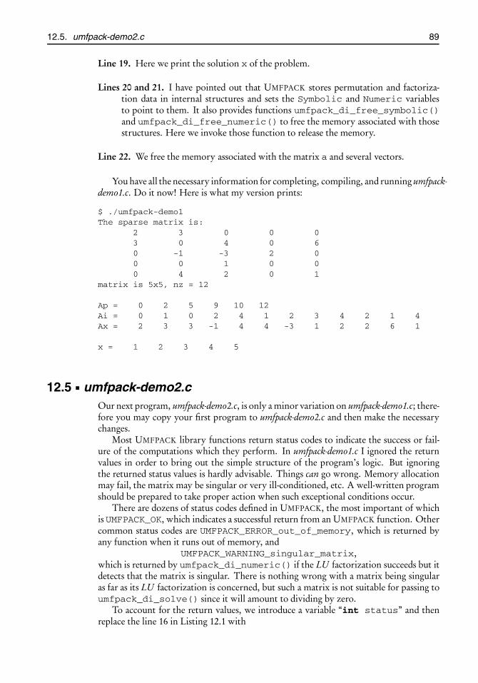
root2014/7/8page 89
�
�
�
�
�
�
�
�
12.5. umfpack-demo2.c 89
Line 19. Here we print the solution x of the problem.
Lines 20 and 21. I have pointed out that UMFPACK stores permutation and factoriza-tion data in internal structures and sets the Symbolic and Numeric variablesto point to them. It also provides functions umfpack_di_free_symbolic()and umfpack_di_free_numeric() to free the memory associated with thosestructures. Here we invoke those function to release the memory.
Line 22. We free the memory associated with the matrix a and several vectors.
You have all the necessary information for completing, compiling, and running umfpack-demo1.c. Do it now! Here is what my version prints:
$ ./umfpack-demo1The sparse matrix is:
2 3 0 0 03 0 4 0 60 -1 -3 2 00 0 1 0 00 4 2 0 1
matrix is 5x5, nz = 12
Ap = 0 2 5 9 10 12Ai = 0 1 0 2 4 1 2 3 4 2 1 4Ax = 2 3 3 -1 4 4 -3 1 2 2 6 1
x = 1 2 3 4 5
12.5 umfpack-demo2.cOur next program, umfpack-demo2.c, is only a minor variation on umfpack-demo1.c; there-fore you may copy your first program to umfpack-demo2.c and then make the necessarychanges.
Most UMFPACK library functions return status codes to indicate the success or fail-ure of the computations which they perform. In umfpack-demo1.c I ignored the returnvalues in order to bring out the simple structure of the program’s logic. But ignoringthe returned status values is hardly advisable. Things can go wrong. Memory allocationmay fail, the matrix may be singular or very ill-conditioned, etc. A well-written programshould be prepared to take proper action when such exceptional conditions occur.
There are dozens of status codes defined in UMFPACK, the most important of whichis UMFPACK_OK, which indicates a successful return from an UMFPACK function. Othercommon status codes are UMFPACK_ERROR_out_of_memory, which is returned byany function when it runs out of memory, and
UMFPACK_WARNING_singular_matrix,which is returned by umfpack_di_numeric() if the LU factorization succeeds but itdetects that the matrix is singular. There is nothing wrong with a matrix being singularas far as its LU factorization is concerned, but such a matrix is not suitable for passing toumfpack_di_solve() since it will amount to dividing by zero.
To account for the return values, we introduce a variable “int status” and thenreplace the line 16 in Listing 12.1 with

root2014/7/8page 90
�
�
�
�
�
�
�
�
90 Chapter 12. Sparse systems: The UMFPACK library
status = umfpack_di_symbolic(n, n, Ap, Ai, Ax, &Symbolic, NULL, NULL);if (status �= UMFPACK_OK) {
fprintf(stderr, "file %s, line %d: umfpack_di_symbolic() failed\n",__FILE__, __LINE__);
return EXIT_FAILURE;}
Padding every occurrence of an UMFPACK function this way results in a lot of clutter.A better strategy is to isolate the error reporting to a function of its own. Here is an idea.Define
static void error_and_exit(int status, const char *file, int line){
fprintf(stderr, "*** file %s, line %d: ", file, line);switch (status) {
case UMFPACK_ERROR_out_of_memory:fprintf(stderr, "out of memory!\n");break;
case UMFPACK_WARNING_singular_matrix:fprintf(stderr, "matrix is singular!\n");break;
default:fprintf(stderr, "UMFPACK error code %d\n", status);
}exit(EXIT_FAILURE);
}
It prints an informative error message to stderr and then calls exit() to terminatethe program. With this function on hand, you may replace line 16 in Listing 12.1 with
status = umfpack_di_symbolic(n, n, Ap, Ai, Ax, &Symbolic, NULL, NULL);if (status �= UMFPACK_OK)
error_and_exit(status, __FILE__, __LINE__);
This is more compact than the previous suggestion.Change lines 17 and 18 in the same way, and then compile and test the program. The
output should be identical to that of the previous version.To check the proper functioning of error_and_exit(), change the matrix A to
a singular one. (You may do that, for instance, by changing the two entries in the firstcolumn to zeros.) Try again. Does your program behave as designed?
12.6 umfpack-demo3.c and the triplet formEach of the two previous demo programs begins with a fully formed matrix A and thencalls sparse_pack() to produce its CCS representation vectors Ap, Ai, and Ax. If youthink about it, this is totally insane! The sole purpose of sparse storage is to avoid wastingmemory in storing a matrix’s zero entries. But what do we do? In the first place, wecommit the sin of storing the entire matrix, zeros and all, in the array A. Then we addinsult to injury by allocating yet more memory for its CCS vectors. That can’t be right,can it? No, it’s not. A proper implementation will have no matrix A at all! It will beginwith a list of A’s nonzero entries only and go from there. Let’s see how.

root2014/7/8page 91
�
�
�
�
�
�
�
�
12.6. umfpack-demo3.c and the triplet form 91
12.6.1 The triplet form
How do we produce a matrix’s nonzero entries without producing the matrix itself? Anonzero entry may be identified as a triplet (i , j , x), where the i and j are the entry’s rowand column indices, and x is its value. A sparse matrix is specified completely by a list ofsuch triplets. There is no need to store the full matrix at all.
Let’s say we wish to store N such triplets. One way is to make a vector of length Nwhose entries are structures that hold triplets. Another way, and this is the way it’s donein UMFPACK, is to make three vectors of length N each, let’s call them Ti, Tj, Tx, andstore the kth triplet as (Ti[k], Tj[k], Tx[k]). Thus, the matrix A of Section 12.4may be encoded as
int N = 20, k = 0; // N = 20 is an overestimate; N = 12 will doint *Ti, *Tj;double *Tx;make_vector(Ti, N);make_vector(Tj, N);make_vector(Tx, N);Ti[k] = 0; Tj[k] = 0; Tx[k] = 2.0; k++; // the (0,0) entry is 2.0Ti[k] = 1; Tj[k] = 0; Tx[k] = 3.0; k++; // the (1,0) entry is 3.0Ti[k] = 0; Tj[k] = 1; Tx[k] = 3.0; k++; // the (0,1) entry is 3.0...
As you see, we are defining the sparse matrix here without constructing the full matrix. InUMFPACK, a representation of a matrix through the Ti, Tj, Tx vectors is called the tripletform of that matrix. Let me point out that the order in which the entries are defined isimmaterial. For instance, the (0,1) entry is 3.0 no matter where it appears in the sequenceof assignments above.
This brings up an issue to ponder: Suppose that we enter
Ti[5] = 3; Tj[5] = 4; Tx[5] = 2.0; // the (3,4) entry is 2.0Ti[8] = 3; Tj[8] = 4; Tx[8] = 9.0; // the (3,4) entry is 9.0
One line says that the matrix’s (3,4) entry is 2.0. The other line says that it is 9.0. Sowhich is it? UMFPACK answers the question by adding the entries! Thus, the two linesshown above are interpreted to mean that the (3,4) entry is 11.0. In general, if an entryis given multiple times, its values accumulate. This is exactly what is needed in finiteelement programs. In Chapter 25, for instance, the matrix A (called the system’s stiffnessmatrix) is constructed piecemeal. The information about its entries becomes available alittle at a time and accumulates, just as in the snippet above.
12.6.2 From the triplet form to CCS
The triplet form is a temporary (but very useful) means of storing a sparse matrix. It needsto be translated to CCS because that’s what UMFPACK’s functions call for. UMFPACK’sumfpack_di_triplet_to_col() function translates from the triplet form to CCS.Thus, suppose that the triplet vectors Ti, Tj, Tx vectors (of length N each) represent ann× n sparse matrix. To obtains A’s CCS representation, we do
make_vector(Ap, n + 1);make_vector(Ai, N);make_vector(Ax, N);status = umfpack_di_triplet_to_col(n, n, N, Ti, Tj, Tx, Ap, Ai, Ax, NULL);if (status �= UMFPACK_OK)
error_and_exit(status, __FILE__, __LINE__);

root2014/7/8page 92
�
�
�
�
�
�
�
�
92 Chapter 12. Sparse systems: The UMFPACK library
The call to umfpack_di_triplet_to_col() reads the triplet vectors Ti, Tj, Txand populates the CCS vectors Ap, Ai, Ax with the corresponding data. The triplet vec-tors are not needed beyond this point, so you may free their memory now.
Remark 12.2. In view of the accumulation effect of the triplet representation, it shouldbe clear that the number of triplets specified in the Ti, Tj, Tx vectors is not the same asthe number of nonzero entries, nz, of the matrix A, which are fewer in general. Had Iknown nz, I would have allocated vectors of lengths nz, rather than N , for Ai and Axin the code fragment above. But generally we don’t know nz ahead of the time, so I usedN instead. That’s an overestimate and a bit wasteful but perhaps not worth fretting overtoo much.
Remark 12.3. Continuing on the issue brought up in the previous remark, recall thatAp[n] equals the number of nonzero entries in a CCS representation. Therefore we cantell a matrix’s true nz value by looking up the number that is stored in Ap[n]. Unfor-tunately that information arrives too late—we need to allocate the vectors Ai and Ax oflength N before calling umfpack_di_triplet_to_col(). Only then we may lookup the value of nz in Ap[n].
12.6.3 umfpack-demo3.c
Copy umfpack-demo2.c to umfpack-demo3.c. Remove the declaration “double **a;”and all references to the matrix a. Remove the header file sparse.h because it’s no longerneeded. In main(), replace the definition of the matrix A by its triplet form. Applyumfpack_di_triplet_to_col() to convert it to CCS. The rest of the file remainsthe same. It solves the system Ax = b and prints the solution, as before.
12.7 Project UMFPACK
Part 12.1. Implement, compile, and test the programs umfpack-demo1.c, umfpack-demo2.c,and umfpack-demo3.c, as discussed in this chapter.
Part 12.2. The matrix A on our programs has an entry of 3.0 in its first column andsecond row. Copy umfpack-demo3.c to umfpack-demo4.c and modify umfpack-demo4.cso that the entry is specified twice: once as 1.0, and once again as 2.0. Entries in thetriplet form accumulate; therefore that change should not affect the result. See if yourprogram confirms that.

root2014/7/8page 93
�
�
�
�
�
�
�
�
Chapter 13
Haar wavelets
Prerequisites: Chapters 7, 8
13.1 A brief backgroundAmong the disconcerting findings in the nascent field of functional analysis in the late 19thcentury was the discovery of continuous functions on a closed interval whose (trigono-metric) Fourier series converged pointwise but not uniformly; see Zygmund [84, The-orem 1.13, p. 300]. The generalization of the classical trigonometric Fourier series tothe geometric abstraction of the Hilbert space in the first decade of the 20th centuryprovided great impetus to study that and related pathological behaviors in a new light.Haar [24, 25], in a dissertation written under Hilbert, constructed a complete orthonor-mal basis for the Hilbert space L2(0,1) with the property that the (generalized) Fourierseries in that basis of any continuous function converged uniformly to that function.This showed that the failure of uniform convergence noted above is due to the choice oftrigonometric functions for the basis, rather than a generic property of all Fourier series.
Haar’s basis functions gained a new-found prominence in the 1980s, where it wasnoted that they formed a very special case of the more general theory of wavelets thatwas being developed then. Thus, they were dubbed Haar wavelets retroactively.
I will not deal with general wavelets in this book. The present exposition is driven bythe ultimate goal of applications to image analysis in Chapter 15. Haar wavelets are suitedparticularly well to that purpose; therefore I will limit the discussion to them.
Much of this chapter’s material comes from the introductory articles of Stollnitz,DeRose, and Salesin [66, 67] that later developed into the book [68]. I have found Niev-ergelt’s book [51] also quite informative and learned the “in place” wavelet transformation(see Section 13.6) from it. Strang’s expository articles [69, 70] make for good readings aswell. For algorithmic and programming issues dealing with general wavelets see [53].
13.2 The space L2(0, 1)I will use the usual notation L2(0,1) for the linear space of square (Lebesgue) integrablereal-valued functions on the interval (0,1). The inner product(·, ·) and the norm ‖ · ‖ inL2(0,1) are defined by
( f , g ) =∫ 1
0f (x)g (x)d x, ‖ f ‖2 = ( f , f ) =
∫ 1
0| f (x)|2 d x, f , g ∈ L2(0,1).
93

root2014/7/8page 94
�
�
�
�
�
�
�
�
94 Chapter 13. Haar wavelets
It can be shown (see, e.g., [48] for a very readable account) that the norm satisfies thetriangle inequality:
‖ f − g‖ ≤ ‖ f − h‖+ ‖h − g‖ for all f , g , h ∈ L2(0,1);
therefore ‖ f − g‖ is a metric, that is, a meaningful measure of “distance” between thefunctions f and g .
The inner product generalizes the idea of the dot product inRn . Thus, the functions fand g are said to be orthogonal in L2(0,1) if ( f , g ) = 0. An orthogonal set� ⊂ L2(0,1) is acollection of functions such that every pair of functions in� is orthogonal. Furthermore,an orthogonal set� is said to be orthonormal if ‖ f ‖= 1 for all f ∈� . Since it is possibleto construct orthonormal sets in L2(0,1) that have arbitrarily many elements, L2(0,1) isan infinite-dimensional space.
In analogy with the decomposition of vectors in Rn along an orthonormal basis, wesay the orthonormal set� = { fi }∞i=1 ⊂ L2(0,1) is a complete orthonormal basis in L2(0,1)if any function f ∈ L2(0,1)may be expressed as
f =∞∑
i=1
( f , fi ) fi = ( f , f1) f1+( f , f2) f2+ · · · , (13.1)
where the convergence of the infinite sum is understood in the sense of the norm ‖·‖. Theinfinite sum here is called the generalized Fourier series of the function f with respect tothe basis� . One of the outcomes of Haar’s 1910 article [24] is the explicit constructionof a basis � of L2(0,1) such that the generalized Fourier series of any continuous func-tion converges not only in the sense of the norm ‖ · ‖ but also uniformly to that function.We will study the details of Haar’s construction in the next section.
13.3 Haar’s constructionPick an integer j ≥ 0, and then partition the interval [0,1] into 2 j subintervals of equallengths through the dividing points with coordinates i/2 j , i = 0,1, . . . , 2 j . Let Vj be theset of piecewise-constant functions on [0,1] whose discontinuities, if any, fall on thosedividing points. Clearly Vj is a linear subspace of L2(0,1). Toward the construction of anorthonormal basis� j in Vj , define φ : R→R as36
φ(x) =
�1 if 0≤ x ≤ 1,0 otherwise,
(13.2)
and for any i = 0,1, . . . , 2 j − 1, set
φ ji (x) = 2 j/2φ(2 j x − i), 0≤ x ≤ 1, (13.3)
and then let � j = {φ ji }2 j−1
i=0 . (The j in φ ji is merely a superscript, not an exponent.) To
understand � j , let us study the set �2 = {φ20,φ2
1,φ22,φ2
3} first. The graphs of�2’s fourfunctions are shown in the top row in Figure 13.1. It should be clear that any functionin V2 may be expressed uniquely as a linear combination of these; therefore �2 is a ba-sis for V2. In particular, the dimension of V2, which is defined as the number of basis
36The values ofφ(x) at x = 0 and x = 1 are irrelevant in wavelet applications and will be ignored. Those wererelevant to Haar, whose aim was to prove the uniform convergence of the generalized Fourier series.

root2014/7/8page 95
�
�
�
�
�
�
�
�
13.3. Haar’s construction 95
0 14
12
34
1
φ20
0 14
12
34
1
φ21
0 14
12
34
1
φ22
0 14
12
34
1
φ23
0
14
12
34
1
ψ20
0 14
12
34
1
ψ21
0 14
12
34
1
ψ22
0 14
12
34
1ψ23
Figure 13.1: The Haar scaling functions {φ20,φ2
1,φ22,φ2
3} form a basis for V2. The Haarwavelets {ψ2
0,ψ21,ψ2
2,ψ23} form a basis for W2. Taken together, the eight
functions form a basis for V3 = V2 ⊕W2. Since j = 2, the height of thenonzero part of each of the functions shown above is 2 j/2 = 2. (These arenot drawn to scale.) All function have unit L2 norms.
elements, is 4. We write that as dimV2 = 4. Moreover, it should also be clear that thefunctions in�2 are orthogonal, that is, (φ2
i1,φ2
i2) =
∫ 10 φ
2i1(x)φ2
i2(x)d x = 0 if i1 �= i2. This
is because the regions where φ2i1
and φ2i2
are nonzero don’t overlap.37 The coefficient 2 j/2
in (13.3) is chosen on purpose so that∫ 1
0
���φ ji (x)
���2 d x =�2 j/2 2× 2− j = 1 for all j .
Thus,�2 is an orthonormal basis in V2.The observations of the previous paragraph regarding V2 generalize in a straightfor-
ward way to Vj for any j ≥ 0. Thus,� j is an orthonormal basis in Vj , and dimVj = 2 j .The spaces Vj form a nested hierarchy of increasingly richer subspaces of L2(0,1):
V0 ⊂V1 ⊂V2 ⊂ · · · ⊂ L2(0,1).
For each j , let Wj be the orthogonal complement of Vj in Vj+1. In other words, Wj is theset of all functions in Vj+1 which are orthogonal to all functions in Vj . That’s written asVj+1 = Vj ⊕Wj . Since dimVj+1 = 2 j+1 = 2× 2 j and dimVj = 2 j , then dimWj = 2 j .We conclude that any function in the 2 j+1-dimensional space Vj+1 may be decomposeduniquely into the sum of two functions in the 2 j -dimensional orthogonal subspaces Vj
and Wj .Toward constructing an orthonormal basis for Wj , let’s define ψ : R→R as38
ψ(x) =
⎧⎪⎨⎪⎩+1 if 0< x < 1
2 ,−1 if 1
2 < x < 1,0 otherwise
37Technical note: The closure of the set where a function is nonzero is called that function’s support. Weare saying that the supports of φ2
i1and φ2
i2don’t overlap. This is not literally true because two such supports
may have a point in common. But integration over a point produces zero; therefore the statement regarding theorthogonality of φ2
i1and φ2
i2still holds.
38As in the case ofφ, the values ofψ at its points of discontinuity are irrelevant in wavelet applications. Haargave them specific values because his aim was to study uniform convergence.

root2014/7/8page 96
�
�
�
�
�
�
�
�
96 Chapter 13. Haar wavelets
and, for any i = 0,1, . . . , 2 j − 1, set
ψ ji (x) = 2 j/2ψ(2 j x − i), 0≤ x ≤ 1. (13.4)
Let �′j = {ψ j
i }2 j−1i=0 . The graphs of the four functions �′
2 = {ψ20,ψ2
1,ψ22,ψ2
3} are shownin the bottom row in Figure 13.1. It is clear that they form an orthogonal set, that is,(ψ2
i1,ψ2
i2) =
∫ 10 ψ
2i1(x)ψ2
i2(x)d x = 0 if i1 �= i2. It is also clear that any of the functions in
the bottom row is orthogonal to any of the function in the top row, that is, (ψ2i1
,φ2i2) =∫ 1
0 ψ2i1(x)ψ2
i2(x)d x = 0 for all i1 and i2. Moreover, the coefficient 2 j in (13.4) is chosen on
purpose so that ‖ψ ji ‖ = 1 for all i and j . Thus, �′
2 is an orthonormal set, and span{�′2}
is orthogonal to V2. Additionally, let us observe that every element of �′2 is in V3. (Do
you see that?)The observations of the previous paragraph regarding the case j = 2 generalize in a
straightforward way to any j ≥ 0. Thus,
a. �′j is an orthonormal set;
b. span{�′j } is orthogonal to Vj ; and
c. span{�′j } ⊂Vj+1.
Recalling that Wj is the orthogonal complement of Vj in Vj+1, it follows that span{�′j } ⊂
Wj . But since span{�′j } has 2 j elements, and since dimWj = 2 j , we conclude that
span{�′j }=Wj , that is,�′
j is an orthonormal basis of Wj .
In the context of the modern theory of wavelets, the basis functionsφ ji of Vj are called
the Haar scaling functions, and the basis functions ψ ji of Wj are called the Haar wavelets
on account of their wiggly graphs; see the graphs in the bottom row in Figure 13.1.For future reference, let us note that the functions 2− j/2φ j
i and 2− j/2ψ ji both are of
amplitude 1; therefore,
2−( j−1)/2φ j−1i = 2− j/2φ j
2i + 2− j/2φ j2i+1,
2−( j−1)/2ψ j−1i = 2− j/2φ j
2i − 2− j/2φ j2i+1.
Solving for φ j−1i and ψ j−1
i we get
φ j−1i =
1�2
�φ j
2i +φj2i+1
, i = 0,1, . . . , 2 j−1 − 1, (13.5a)
ψ j−1i =
1�2
�φ j
2i −φ j2i+1
, i = 0,1, . . . , 2 j−1 − 1. (13.5b)
These express the basis functions of Vj−1 and Wj−1 as linear combination of the basisfunctions of Vj . In effect, these are the concrete realizations of the decomposition Vj =Vj−1 ⊕Wj−1. Figure 13.2 is an attempt to express this in a schematic diagram. Try tomake a sense of it.

root2014/7/8page 97
�
�
�
�
�
�
�
�
13.4. The decomposition Vj =Vj−1⊕Wj−1 97
V1 = span{φ10,φ1
1}
W1=
span{ψ
1 0,ψ1 1}
span{φ
20,φ
21}span{φ 2
2 ,φ 23 }
V1 = span{φ10,φ1
1}W1 = span{ψ1
0,ψ11}
V2 = span{φ20,φ2
1,φ22,φ2
3}=V1⊕W1
Figure 13.2: This schematic diagram is an attempt to illustrate the decomposition V2 =V1 ⊕W1. The circle represents the four-dimensional space V2. The hori-zontal and vertical lines represent the two-dimensional mutually orthog-onal subspaces V1 = span{φ1
0,φ11} and W1 = span{ψ1
0,ψ11}. The dashed
lines represent V2’s natural basis {φ20,φ2
1,φ22,φ2
3}. Their rotated positionsemphasize that they are not aligned with the spaces V1 and W1. Equa-tions (13.5a) and (13.5b) give the rotation equations that relate the solidand dashed spaces.
13.4 The decomposition Vj =Vj−1⊕Wj−1
Let us introduce the notation
α ji = ( f ,φ j
i ), β ji = ( f ,ψ j
i ), where f ∈ L2(0,1). (13.6)
In view of (13.5a) and (13.5b), we have
α j−1i = ( f ,φ j−1
i ) =�
f ,1�2
�φ j
2i +φj2i+1
�=
1�2
�α j
2i +αj2i+1
,
β j−1i = ( f ,ψ j−1
i ) =�
f ,1�2
�φ j
2i −φ j2i+1
�=
1�2
�α j
2i −α j2i+1
.
This is a very significant result—it expresses the components of f along the bases � j−1
and �′j−1 in terms of those along the basis � j , and thus it offers yet another way of
viewing the decomposition Vj =Vj−1⊕Wj−1. Let us state it formally as a theorem.
Theorem 13.1. For any function f ∈Vj , the components α ji andβ j
i defined in (13.6) satisfythe recursive relations
α j−1i =
1�2
�α j
2i +αj2i+1
, i = 0,1, . . . , 2 j−1− 1, (13.7a)
β j−1i =
1�2
�α j
2i −α j2i+1
, i = 0,1, . . . , 2 j−1− 1. (13.7b)
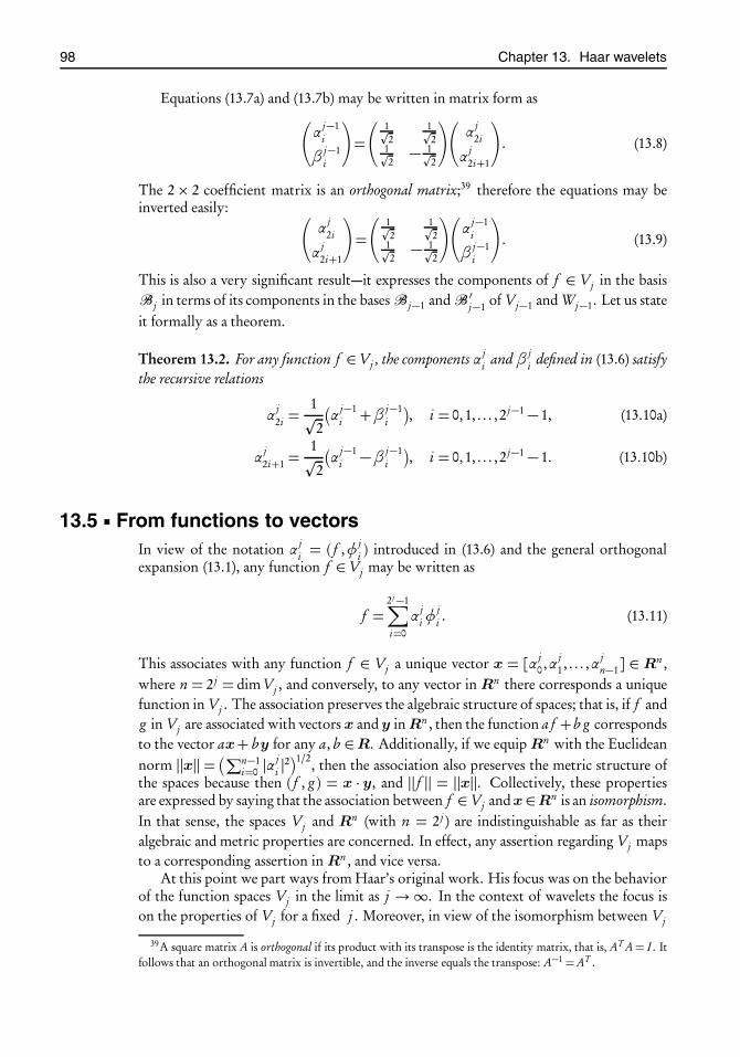
root2014/7/8page 98
�
�
�
�
�
�
�
�
98 Chapter 13. Haar wavelets
Equations (13.7a) and (13.7b) may be written in matrix form as�α j−1
i
β j−1i
�=
�1�2
1�2
1�2− 1�
2
��α j
2i
α j2i+1
�. (13.8)
The 2× 2 coefficient matrix is an orthogonal matrix;39 therefore the equations may beinverted easily: �
α j2i
α j2i+1
�=
�1�2
1�2
1�2− 1�
2
��α j−1
i
β j−1i
�. (13.9)
This is also a very significant result—it expresses the components of f ∈ Vj in the basis� j in terms of its components in the bases� j−1 and�′
j−1 of Vj−1 and Wj−1. Let us stateit formally as a theorem.
Theorem 13.2. For any function f ∈Vj , the components α ji andβ j
i defined in (13.6) satisfythe recursive relations
α j2i =
1�2
�α j−1
i +β j−1i
, i = 0,1, . . . , 2 j−1 − 1, (13.10a)
α j2i+1 =
1�2
�α j−1
i −β j−1i
, i = 0,1, . . . , 2 j−1 − 1. (13.10b)
13.5 From functions to vectorsIn view of the notation α j
i = ( f ,φ ji ) introduced in (13.6) and the general orthogonal
expansion (13.1), any function f ∈Vj may be written as
f =2 j−1∑i=0
α jiφ
ji . (13.11)
This associates with any function f ∈ Vj a unique vector x = [α j0,α j
1, . . . ,α jn−1] ∈ Rn ,
where n = 2 j = dimVj , and conversely, to any vector in Rn there corresponds a uniquefunction in Vj . The association preserves the algebraic structure of spaces; that is, if f andg in Vj are associated with vectors x and y in Rn , then the function a f +b g correspondsto the vector ax+ by for any a, b ∈R. Additionally, if we equip Rn with the Euclideannorm ‖x‖ = �∑n−1
i=0 |α ji |2 1/2, then the association also preserves the metric structure of
the spaces because then ( f , g ) = x · y, and ‖ f ‖ = ‖x‖. Collectively, these propertiesare expressed by saying that the association between f ∈Vj andx ∈Rn is an isomorphism.In that sense, the spaces Vj and Rn (with n = 2 j ) are indistinguishable as far as theiralgebraic and metric properties are concerned. In effect, any assertion regarding Vj mapsto a corresponding assertion in Rn , and vice versa.
At this point we part ways from Haar’s original work. His focus was on the behaviorof the function spaces Vj in the limit as j →∞. In the context of wavelets the focus ison the properties of Vj for a fixed j . Moreover, in view of the isomorphism between Vj
39A square matrix A is orthogonal if its product with its transpose is the identity matrix, that is, AT A= I . Itfollows that an orthogonal matrix is invertible, and the inverse equals the transpose: A−1 =AT .

root2014/7/8page 99
�
�
�
�
�
�
�
�
13.5. From functions to vectors 99
and Rn , our study will shift gradually from the function spaces Vj to the correspondingvector spaces Rn . That shift is very evident in the following discussion.
Let us illustrate Theorems 13.1 and 13.2 in the case j = 3. Since V3 = V2 ⊕W2,then an f ∈ V3 may be expressed in two ways: (a) as a linear combination of the basisfunctions�3, or (b) as the sum of a linear combinations of the bases �2 and�′
2:
f = α30φ
30+α
31φ
31+α
32φ
32+α
33φ
33+α
34φ
34+α
35φ
35+α
36φ
36+α
37φ
37,
f =�α2
0φ20+α
21φ
21+α
22φ
22+α
23φ
23
+�β2
0ψ20+β
21ψ
21+β
22ψ
22+β
23ψ
23
.
The first representation is associated with the vector�α3
0 α31 α3
2 α33 α3
4 α35 α3
6 α37
�(13.12)
in R8. The second representation is associated with the pair of vectors [α20,α2
1,α22,α2
3] and[β2
0,β21,β2
2,β23] in R4. Let us merge the latter two vectors into a single vector in R8 by
alternating their components, as in�α2
0 β20 α2
1 β21 α2
2 β22 α2
3 β23
�. (13.13)
Theorems 13.1 and 13.2 establish the transformation rule between the vectors (13.12)and (13.13). Specifically, according to Theorems 13.1,⎛⎜⎜⎜⎜⎜⎜⎜⎜⎜⎜⎜⎜⎜⎜⎜⎝
α20
β20
α21
β21
α22
β22
α23
β23
⎞⎟⎟⎟⎟⎟⎟⎟⎟⎟⎟⎟⎟⎟⎟⎟⎠=
⎛⎜⎜⎜⎜⎜⎜⎜⎜⎜⎜⎜⎜⎜⎜⎝
1�2
1�2
1�2− 1�
21�2
1�2
1�2− 1�
21�2
1�2
1�2− 1�
21�2
1�2
1�2− 1�
2
⎞⎟⎟⎟⎟⎟⎟⎟⎟⎟⎟⎟⎟⎟⎟⎠
⎛⎜⎜⎜⎜⎜⎜⎜⎜⎜⎜⎜⎜⎜⎜⎝
α30
α31
α32
α33
α34
α35
α36
α37
⎞⎟⎟⎟⎟⎟⎟⎟⎟⎟⎟⎟⎟⎟⎟⎠.
Only the nonzero entries of the coefficient matrix are shown. The matrix’s block-diagonalstructure indicates that the transformation is local in the sense that the first pair of com-ponents in (13.13) is determined by the first pair in (13.12). Similarly, the second pairof components in (13.13) is determined by the second pair in (13.12), and so on. Thus,transforming the vector (13.12) to (13.13) may be performed by a “moving window” ofwidth 2 as follows:
α30 α3
1 α32 α3
3 α34 α3
5 α36 α3
7
α20 β2
0 α21 β2
1 α22 β2
2 α23 β2
3
the vector (13.12)→
the vector (13.13)→moving window
Here, within each window the entries in the top corners determine the entries in the bot-tom corners (Theorem 13.1), and conversely, the entries in the bottom corners determinethe entries in the top corners (Theorem 13.2).

root2014/7/8page 100
�
�
�
�
�
�
�
�
100 Chapter 13. Haar wavelets
0 14
12
34
1
φ00
0 14
12
34 1ψ0
0
0
14
12
34 1ψ1
0
0 14
12
34
1ψ11
0
14
12
34
1
ψ20
0 14
12
34
1
ψ21
0 14
12
34
1
ψ22
0 14
12
34
1ψ23
Figure 13.3: The wavelet basis �3 = {φ00,ψ
00,ψ1
0,ψ10,ψ2
0,ψ21,ψ2
2,ψ23} of the eight-
dimensional space V3 shown to scale. The amplitudes of the first two are2 j/2 = 20/2 = 1. The amplitudes of the next two are 2 j/2 = 21/2 =
�2. The
amplitudes of the last four are 2 j/2 = 22/2 = 2. All function have unit L2
norms.
13.6 The Haar wavelet transformWe have seen that Vj = Vj−1 ⊕Wj−1. By the same token, Vj−1 = Vj−2 ⊕Wj−2. Substi-tuting the Vj−1 from the second equation into the first, we get Vj =Vj−2⊕Wj−2⊕Wj−1.By applying this idea repeatedly, we reduce V ’s index on the right-hand side to zero andarrive at
Vj =V0⊕W0⊕W1⊕ · · · ⊕Wj−1. (13.14)
This expression is called the wavelet decomposition of the space Vj . The union of the basesof the individual parts,� j =�0∪�′
0∪�′1∪· · ·∪�′
j−1, is an orthonormal basis in Vj andis called the Haar wavelet basis of the space Vj . When a function f ∈Vj is expressed as alinear combination of the Haar wavelet basis, the coefficients of that linear combinationare called the function’s Haar wavelet coefficients. For instance, if f ∈ V3 = V0 ⊕W0 ⊕W1⊕W2, then
f = α00 φ
00︸ ︷︷ ︸
∈V0
+β00 ψ
00︸ ︷︷ ︸
∈W0
+β10 ψ
10+β
11 ψ
11︸ ︷︷ ︸
∈W1
+β20 ψ
20+β
21 ψ
21+β
22 ψ
22+β
23 ψ
23︸ ︷︷ ︸
∈W2
and the wavelet coefficients are [α00,β0
0,β10,β1
1,β20,β2
1,β22,β2
3]. Figure 13.3 shows thegraphs of the Haar wavelet basis functions in �3. The purpose of the rest of this section isto obtain a simple algorithm for computing the Haar wavelet coefficients of functions f ∈Vjfor any j .
Remark 13.1. The space V0 consists of constant functions on the interval [0,1]. Eachwavelet in Wi is a function of zero average. Therefore in the decomposition (13.14) thecomponent in V0 picks up f ’s average over the interval [0,1]. The wavelet componentsadd progressively finer details to that average and ultimately reconstruct f .
13.6.1 Computing the wavelet coefficients
Theorem 13.1 tells us how to decompose Vj into Vj−1 ⊕Wj−1. The full wavelet decom-position in (13.14) is a matter of repeated application of that theorem. I will explain the

root2014/7/8page 101
�
�
�
�
�
�
�
�
13.6. The Haar wavelet transform 101
α40 α4
1 α42 α4
3 α44 α4
5 α46 α4
7 α48 α4
9 α410 α4
11 α412 α4
13 α414 α4
15
α30 β3
0 α31 β3
1 α32 β3
2 α33 β3
3 α34 β3
4 α35 β3
5 α36 β3
6 α37 β3
7
α20 β2
0 α21 β2
1 α22 β2
2 α23 β2
3
α10 β1
0 α11 β1
1
α00 β0
0
1.
2.
3.
4.
5.
Figure 13.4: Rows 1 through 5 show the various stages of an in place Haar transform ofan f ∈V4. Row 1 is the vector of the 16 coefficients of the expansion of fin the basis�4. To reduce clutter, only the vector’s changed elements areshown in each row. Blanks indicate values that are to be carried over froma previous row.
procedure in the case of j = 4, that is,
V4 =V0⊕W0⊕W1⊕W2⊕W3.
The generalization to arbitrary j should should be evident.Figure 13.4 illustrates the algorithm. It begins with a function f =
∑15i=0 α
4iφ
4i ∈V 4.
The associated vector in R16, that is,�α4
0 α41 α4
2 α43 α4
4 α45 α4
6 α47 α4
8 α49 α4
10 α411 α4
12 α413 α4
14 α415
�,
(13.15)
is entered in row 1 in Figure 13.4. The algorithm that I will describe changes that vectorinto its Haar wavelet transform in place; that is, the vector is overwritten by the trans-form. No extra storage is required. Rows 1 through 5 show the successive stages of theconversion of that vector. To eliminate clutter, each row shows only the parts of the vec-tor that are changed relative to the previous row. The unchanged parts are left blank. Forinstance, there are only two changed entries in row 5. The remaining 14 entries (whichare not shown) are as they were in the previous rows.
The procedure begins with the “moving window” idea, described in the previous sec-tion, applied to the vector of row 1 to produce the vector of row 2. This amounts to thedecomposition V4 = V3 ⊕W3. The α3
i and β3i in row 2 are the components of f in V3
and W3. The α3i entries await further work since V3 is to be decomposed into V2 ⊕W2.
The β3i entries are finalized at this stage. In the subsequent rows their positions are left
blank to indicate that their previous values carry over.The moving window that takes us from row 2 to row 3 moves in steps of 4 because
it is interested in the α3i coefficients only—it skips over the β3
i ’s. Similarly, the movingwindow that takes us from row 3 to row 4 moves in steps of 8. Finally the moving windowthat takes us from row 4 to row 5 moves in steps of 16, so it doesn’t move at all. It finalizesthe coefficients α0
0 andβ00 and ends the process. The overall outcome of the process is the
vector�α0
0 β30 β2
0 β31 β1
0 β32 β2
1 β33 β0
0 β34 β2
2 β35 β1
1 β36 β2
3 β37
�.
(13.16)

root2014/7/8page 102
�
�
�
�
�
�
�
�
102 Chapter 13. Haar wavelets
The transformation of the vector (13.15) into (13.16) is called the Haar wavelet trans-form on V4. The transformation may be reversed since every step of the procedure isreversible. Going from (13.16) to (13.15) is called the inverse Haar wavelet transform.
13.6.2 An extra twist
Throughout this section I have worked with functions f ∈Vj expressed in the basis � jof Vj , as in (13.11). In practice, however, a function f ∈ Vj is not given in terms of the� j basis. It is more likely given as a list of values that it takes on the 2 j subintervals ofthe interval [0,1], as in
f (x) = ci 2− j i < x < 2− j (i + 1), i = 0,1, . . . , 2 j − 1.
So to get started with the transformation algorithms described earlier, the first step wouldbe to calculate the coefficients α j
i from the values ci . This is quite easy, actually. Since theamplitude of each φ j
i is 2 j/2, then c j and α ji are related through c j = 2 j/2α j
i , or equiva-lently,
α ji =
1�dimVj
c j , (13.17)
because dimVj = 2 j . In words, the coefficients α j0,α j
1, . . . of the expansion of f in the� j
basis of Vj are obtained simply by dividing the list of the f ’s values by�
dimVj .
13.7 Functions of two variablesThe study of the previous sections led to the construction of the wavelet basis� j of piece-wise constant functions defined on the interval [0,1] partitioned into 2 j equal subinter-vals. Figure 13.3 shows the 23 = 8 members of�3.
The two-dimensional generalization partitions the square [0,1]2 through a uniform2 j1×2 j2 rectangular grid, where j1 and j2 are nonnegative integers, and considers functionsf : (x, y) ∈ [0,1]2 →R which are constant on each cell of the grid.
A basis for the resulting function space is given by the functions
� j1, j2=�
h(x, y) = f (x)g (y) : f ∈� j1, g ∈� j2
.
Figure 13.5 shows the 16 elements of the basis�2,2 from two different perspectives.The theory of wavelets in two dimensions—indeed, in n dimensions—proceeds along
lines similar to what we have seen in one dimension. I will not go through the detailshere but will refer you to the very readable accounts in [68] and [51]. After all is saidand done, it turns out that computing the Haar wavelet transform of functions in twodimensions reduces to the following. Represent the function f (x, y) as a 2 j1 × 2 j2 matrixA which holds the (constant) values of f on the cells of the grid described above. Thendo the following:
• Apply the one-dimensional Haar wavelet transform to every row of the matrix A.Let T be the resulting matrix.
• Apply the one-dimensional Haar wavelet transform to every column of the ma-trix T . The result is the Haar transform of A.
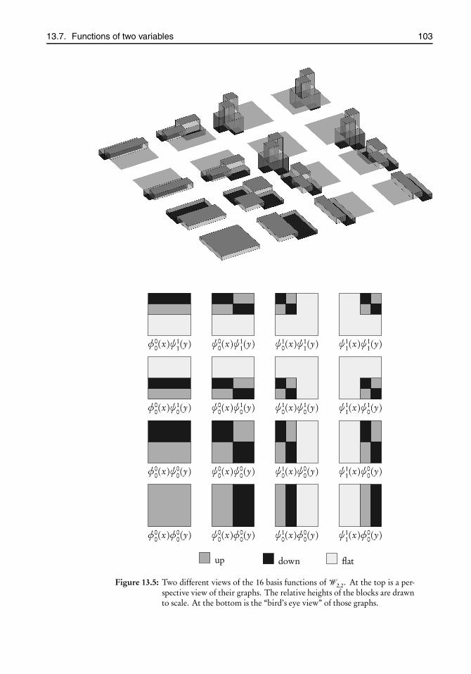
root2014/7/8page 103
�
�
�
�
�
�
�
�
13.7. Functions of two variables 103
φ00(x)φ
00(y) ψ0
0(x)φ00(y) ψ1
0(x)φ00(y) ψ1
1(x)φ00(y)
φ00(x)ψ
00(y) ψ0
0(x)ψ00(y) ψ1
0(x)ψ00(y) ψ1
1(x)ψ00(y)
φ00(x)ψ
10(y) ψ0
0(x)ψ10(y) ψ1
0(x)ψ10(y) ψ1
1(x)ψ10(y)
φ00(x)ψ
11(y) ψ0
0(x)ψ11(y) ψ1
0(x)ψ11(y) ψ1
1(x)ψ11(y)
up down flat
Figure 13.5: Two different views of the 16 basis functions of �2,2. At the top is a per-spective view of their graphs. The relative heights of the blocks are drawnto scale. At the bottom is the “bird’s eye view” of those graphs.
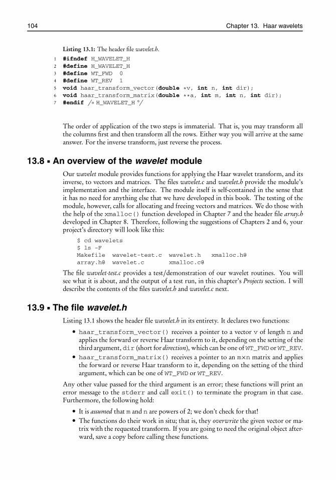
root2014/7/8page 104
�
�
�
�
�
�
�
�
104 Chapter 13. Haar wavelets
Listing 13.1: The header file wavelet.h.
1 #ifndef H_WAVELET_H2 #define H_WAVELET_H3 #define WT_FWD 04 #define WT_REV 15 void haar_transform_vector(double *v, int n, int dir);6 void haar_transform_matrix(double **a, int m, int n, int dir);7 #endif /∗ H_WAVELET_H */
The order of application of the two steps is immaterial. That is, you may transform allthe columns first and then transform all the rows. Either way you will arrive at the sameanswer. For the inverse transform, just reverse the process.
13.8 An overview of the wavelet moduleOur wavelet module provides functions for applying the Haar wavelet transform, and itsinverse, to vectors and matrices. The files wavelet.c and wavelet.h provide the module’simplementation and the interface. The module itself is self-contained in the sense thatit has no need for anything else that we have developed in this book. The testing of themodule, however, calls for allocating and freeing vectors and matrices. We do those withthe help of the xmalloc() function developed in Chapter 7 and the header file array.hdeveloped in Chapter 8. Therefore, following the suggestions of Chapters 2 and 6, yourproject’s directory will look like this:
$ cd wavelets$ ls -FMakefile wavelet-test.c wavelet.h [email protected]@ wavelet.c xmalloc.c@
The file wavelet-test.c provides a test/demonstration of our wavelet routines. You willsee what it is about, and the output of a test run, in this chapter’s Projects section. I willdescribe the contents of the files wavelet.h and wavelet.c next.
13.9 The file wavelet.hListing 13.1 shows the header file wavelet.h in its entirety. It declares two functions:
• haar_transform_vector() receives a pointer to a vector v of length n andapplies the forward or reverse Haar transform to it, depending on the setting of thethird argument, dir (short for direction), which can be one of WT_FWD or WT_REV.
• haar_transform_matrix() receives a pointer to an m×n matrix and appliesthe forward or reverse Haar transform to it, depending on the setting of the thirdargument, which can be one of WT_FWD or WT_REV.
Any other value passed for the third argument is an error; these functions will print anerror message to the stderr and call exit() to terminate the program in that case.Furthermore, the following hold:
• It is assumed that m and n are powers of 2; we don’t check for that!• The functions do their work in situ; that is, they overwrite the given vector or ma-
trix with the requested transform. If you are going to need the original object after-ward, save a copy before calling these functions.

root2014/7/8page 105
�
�
�
�
�
�
�
�
13.10. The file wavelet.c 105
Listing 13.2: An outline of the file wavelet.c.
1 #include <stdio.h>2 #include <stdlib.h>3 #include <math.h>4 #include "wavelet.h"5 #define SQRT1_2 sqrt(1.0/2)6 � static void haar_transform_vector_forward(double *v, int n) ...7 � static void haar_transform_vector_reverse(double *v, int n) ...8 � static void haar_transform_matrix_forward(double **a, int m, int n) ...9 � static void haar_transform_matrix_reverse(double **a, int m, int n) ...
10 � void haar_transform_vector(double *v, int n, int dir) ...11 � void haar_transform_matrix(double **a, int m, int n, int dir) ...
Remark 13.2. The values 0 and 1 of the preprocessor symbol WT_FWD or WT_REVdefined in wavelet.h are not significant; any two distinct integers will do.
13.10 The file wavelet.cListing 13.2 shows an outline of the file wavelet.c. The math.h header file is included toprovide a declaration of the C library function sqrt(), which is used in several placesin the code. The special case of 1/
�2 is handled separately by assigning it to a macro
named SQRT1_2. An optimizing compiler will recognize that SQRT1_2 evaluates to aconstant and therefore will replace all occurrences of SQRT1_2 in the program with thecorresponding numerical value at the time when the program is compiled. Gcc works thatway. If your compiler doesn’t, then it may evaluate 1/
�2 thousands of times during the
program’s execution and thus degrade its performance. If you face that problem, changethe definition of SQRT1_2 to
#define SQRT1_2 0.70710678118654752440 /* sqrt(1.0/2) */
The implementation’s front end is provided by the two functions defined on lines 10and 11, which we met in the previous section. These enlist the help of the four functionsdefined on lines 6 through 9, which do the real work, that is, apply the forward or reverseHaar wavelet transform to vectors and matrices. Their names clearly indicate which doeswhat. All four functions are specified static, and thus they are not accessible fromoutside wavelet.c.
13.10.1 The function haar_transform_vector()
The implementation of haar_transform_vector() that appears on line 10 of List-ing 13.2 is quite straightforward; it is shown in its entirety in Listing 13.3. You will writethe equally simple haar_transform_matrix(), which appears on line 11.
13.10.2 The function haar_transform_vector_forward()
The function haar_transform_vector_forward() that appears on line 6 of List-ing 13.2 receives a pointer v to a vector of length n and applies the algorithm ofSection 13.6 to convert that vector to the corresponding Haar wavelet transform. Thefunction is destructive in the sense that it overwrites the original vector, but it has the
root2014/7/8page 106
�
�
�
�
�
�
�
�
106 Chapter 13. Haar wavelets
Listing 13.3: The function haar_transform_vector() calls one of two auxiliary functionsto do the real transformation work. It expects to be called with the third argument setto one ofWT_FWD orWT_REV; otherwise it prints an error message and callsexit().
1 void haar_transform_vector(double *v, int n, int dir)2 {3 if (dir == WT_FWD)4 haar_transform_vector_forward(v, n);5 else if (dir == WT_REV)6 haar_transform_vector_reverse(v, n);7 else { // shouldn’t be here!8 fprintf(stderr, "*** error in haar_transform_vector(): "9 "the third argument should be one of "
10 "WT_FWD or WT_REV\n");11 exit(EXIT_FAILURE);12 }13 }
Listing 13.4: The function haar_transform_vector_forward().
1 static void haar_transform_vector_forward(double *v, int n)2 {3 double h = sqrt(n);4 int i, d;5 for (i = 0; i < n; i++)6 v[i] /= h;7 for (d = 1; d < n; d *= 2)8 for (i = 0; i < n; i += 2*d) {9 double x = SQRT1_2 * (v[i] + v[i+d]);
10 double y = SQRT1_2 * (v[i] - v[i+d]);11 v[i] = x;12 v[i+d] = y;13 }14 }
advantage of not requiring extra storage to do its work. The length of the vector, n, isassumed to be a power of 2; the function does not check for that!
Before getting into the details of the function’s implementation, let us recall the discus-sion in Section 13.5 regarding the isomorphism between (piecewise constant) functionsin Vj and vectors in Rn , where n = 2 j .
A function in f ∈ Vj is identified by the values it take on the 2 j subintervals of theinterval of [0,1]. Those values form a vector v = [c0, c1, . . . , c2 j−1], which is what thefunction haar_transform_vector_forward() receives. The first order of thingsis to apply the formula (13.17) (page 102) to calculate the components α j
i of f in Vj . The
rest of the algorithm deals with the α ji coefficients.
The complete implementation of the function is shown in Listing 13.4. Note theapplication of the formula (13.17) at the very outset on line 6.
The transformation algorithm begins on line 7. The index d begins with 1 and doublesits value on each iteration. For instance, when n = 16, as in the example of Figure 13.4on page 101, then d takes on the values 1, 2, 4, 8. These correspond, respectively, to

root2014/7/8page 107
�
�
�
�
�
�
�
�
13.10. The file wavelet.c 107
transforming lines 1 to 2, 2 to 3, 3 to 4, and 4 to 5 in that figure. The inner loop on line 8moves the “moving windows” within each row in steps of 2d . The width of the windowis d + 1.
To understand lines 9 and 10, let us focus on the specific case of d = 4 and i = 0.This corresponds to the first of the two moving windows that straddle lines 3 and 4 ofFigure 13.4. (The other window on that row corresponds to the next value of i whichis 2d , that is, 8.) It’s the job of that window to read the values of α2
0 and α21 (at its upper
corners) and compute the values of α10 andβ1
0 (at its lower corners) through the formulas(13.7a) and (13.7b) in Theorem 13.1. Note that α2
0 is located at the 0th place (which is theith place) in vector v, and α2
1 is located at the 4th place (which is the (i + d )th place) invector v. This, together with Theorem 13.1, should explain the calculations on lines 9and 10. Subsequently, on lines 11 and 12, the calculated values are inserted in the ith and(i + d )th places in the vector v, completing that step of the moving window’s operation.
Something to think about: Why are the calculations on lines 9 and 10 separated from theinsertions on lines 11 and 12? What if we do away with the intermediate x and y andcollapse those four lines into two:
v[i] = SQRT1_2 * (v[i] + v[i+d]);v[i+d] = SQRT1_2 * (v[i] - v[i+d]);
Is there anything wrong with that?
13.10.3 The function haar_transform_vector_reverse()
The function haar_transform_vector_reverse() that appears on line 7 of List-ing 13.2 implements the inverse Haar wavelet transform—it receives a pointerv to a vectorof length n and applies the algorithm of Section 13.6 in reversed steps. The function isdestructive in the sense that it overwrites the original vector, but it has the advantage ofnot requiring extra storage to do its work. The length of the vector, n, is assumed to be apower of 2. The function does not check for it!
The successive applications of haar_transform_vector_forward() followedby haar_transform_vector_reverse() to a vector should leave that vector un-changed (other than inaccuracies due to floating point arithmetic).
I will leave it to you to implement haar_transform_vector_reverse(). It’sa matter of reversing the order of computations of Listing 13.4. Let me point out thatlines 9 and 10, which reflect Theorem 13.1, should be replaced, in principle, by thosefrom Theorem 13.2. However, upon a closer scrutiny we see that the transformationmatrices in (13.8) and (13.9) are identical! As a result, lines 9 through 12 of Listing 13.4carry over without change to the new function.
13.10.4 The function haar_transform_matrix_forward()
Following the ideas introduced in Section 13.7, consider a partitioning of the square[0,1]× [0,1] into an m×n grid of identical rectangular cells, where n = 2 j1 and m = 2 j2
for some nonnegative integers j1 and j2. A piecewise constant function on that gird is iden-tified by the m×n matrix of the values that it takes on the grid’s cells. In Section 13.7 welearned that the Haar wavelet transform of such a function is obtained by applying theone-dimensional Haar wavelet transform to every row and then to every column of thematrix.
The function haar_transform_matrix_forward() that appears on line 8 ofListing 13.2 receives a pointer a to such an m×n matrix and overwrites the matrix with

root2014/7/8page 108
�
�
�
�
�
�
�
�
108 Chapter 13. Haar wavelets
the corresponding Haar wavelet transform. It expects m and n to be powers of 2; it doesnot check for that!
At first glance, the implementation of haar_transform_matrix_forward()appears to be trivial; it’s a matter of passing the matrix’s rows and columns to the one-dimensional haar_transform_vector(), as in
for (i = 0; i < m; i++) // transform rowshaar_transform_vector(a[i], n, WT_FWD);
for (j = 0; j < n; j++) // transform columnshaar_transform_vector(... column j (how?) ...);
We see that transforming the rows is trivial indeed since a[i] points to the vector thatmakes up the matrix’s row i . Transforming the columns is not so straightforward becausethe matrix’s columns cannot be accessed as vectors.
There are at least two ways around this difficulty. One way is to set aside an auxiliaryvector of length m, copy the values of the matrix’s column j into the vector, pass thevector tohaar_transform_vector(), and then copy the values from the vector backinto the matrix:
for (i = 0; i < m; i++) // transform rowshaar_transform_vector(a[i], n, WT_FWD);
for (j = 0; j < n; j++) { // transform columnsfor (i = 0; i < m; i++) // step 1: copy column to tmp
tmp[i] = a[i][j];haar_transform_vector(tmp, m, WT_FWD); // step 2: transform tmpfor (i = 0; i < m; i++) // step 3: copy tmp to column
a[i][j] = tmp[i];}
Another way of transforming columns is to forgo haar_transform_vector()altogether. Instead, duplicate the code from haar_transform_vector() and cus-tomize it for the specific purpose of transforming matrix columns:
for (i = 0; i < m; i++) // transform rowshaar_transform_vector(a[i], n, WT_FWD);
h = sqrt(m); // transform columnsfor (j = 0; j < n; j++) {
// customized version of haar_transform_vector()for (i = 0; i < m; i++)
a[i][j] /= h;for (d = 1; d < m; d*=2)
for (i = 0; i < m; i += 2*d) {double x = SQRT1_2 * (a[i][j] + a[i+d][j]);double y = SQRT1_2 * (a[i][j] - a[i+d][j]);a[i][j] = x;a[i+d][j] = y;
}}
I don’t have a strong preference of one method over the other. The first method hasa cleaner code, as it relies entirely on haar_transform_vector() to do its work.However, it requires allocating and freeing an auxiliary vector. Furthermore, the back-and-forth copying of the matrix’s columns into the auxiliary vector is ugly and wasteful.The second method avoids those disadvantages; however, the wisdom of the code dupli-cation is questionable and certainly ugly. I leave it to you to decide between the two

root2014/7/8page 109
�
�
�
�
�
�
�
�
13.11. Project Wavelets 109
methods. Pick one, and write a haar_transform_matrix_forward() for yourwavelet.c.
13.10.5 The function haar_transform_matrix_reverse()
The function haar_transform_matrix_reverse() that appears on line 9 of List-ing 13.2 implements the two-dimensional inverse Haar wavelet transform—it receives apointer a to an m×n matrix and applies the one-dimensional inverse wavelet transformto every column and then to every row. The result overwrites the original matrix. Itexpects m and n to be powers of 2; it does not check for that! There is not much else I canadd regarding this function; it’s just like the forward transform.
13.11 Project WaveletsYour wavelets module should be ready to test now. We are going to write a test/demoprogram, let’s call it wavelet-test.c, to exercise that module and verify that it works cor-rectly. Listing 13.5 gives an outline of wavelet-test.c. The function test_vector()that begins on line 4 makes a vector of length n (assuming n is a power of 2) and setsits entries to vi =
11+i , i = 0,1, . . . . It prints the vector to stdout, then it applies the
Haar wavelet transform to it and prints the result, and then it applies the inverse Haarwavelet transform to it and prints the result again. If the program works correctly, thenthe first and third vectors will be the same. Vectors and matrices are printed by callingprint_vector() and print_matrix() defined in Chapter 8’s array.h.
The functiontest_matrix() on line 28 performs a similar test on matrices. Specif-ically, test_matrix()makes an m×n matrix (assuming that m and n are powers of 2),sets its entries to ai j =
11+i+ j , and then prints the matrix, its wavelet transform, and its in-
verse wavelet transform. If the program works correctly, then the first and third matriceswill be the same. Listing 13.6 shows the output of my version of the program.

root2014/7/8page 110
�
�
�
�
�
�
�
�
110 Chapter 13. Haar wavelets
Listing 13.5: An outline of wavelet-test.c.
1 #include <stdio.h>2 #include "array.h"3 #include "wavelet.h"4 static void test_vector(int n)5 {6 double *v;7
8 make_vector(v, n);9 for (int i = 0; i < n; i++)
10 v[i] = 1.0/(1+i);11
12 printf("original vector:\n");13 print_vector("%8.4f ", v, n);14 putchar(’\n’);15
16 haar_transform_vector(v, n, WT_FWD);17 printf("transformed vector:\n");18 print_vector("%8.4f ", v, n);19 putchar(’\n’);20
21 haar_transform_vector(v, n, WT_REV);22 printf("reconstructed vector:\n");23 print_vector("%8.4f ", v, n);24 putchar(’\n’);25
26 free_vector(v);27 }28 � static void test_matrix(int m, int n)29 {30 ... a[i][j] = 1.0/(1+i+j) ...31 }32 int main(void)33 {34 test_vector(8); // test an 8-vector35 test_matrix(4,8); // test a 4×8 matrix36 return 0;37 }

root2014/7/8page 111
�
�
�
�
�
�
�
�
13.11. Project Wavelets 111
Listing 13.6: The output of wavelet-test.
original vector:1.0000 0.5000 0.3333 0.2500 0.2000 0.1667 0.1429 0.1250
transformed vector:0.3397 0.1250 0.1620 0.0208 0.1811 0.0083 0.0175 0.0045
reconstructed vector:1.0000 0.5000 0.3333 0.2500 0.2000 0.1667 0.1429 0.1250
original matrix:1.0000 0.5000 0.3333 0.2500 0.2000 0.1667 0.1429 0.12500.5000 0.3333 0.2500 0.2000 0.1667 0.1429 0.1250 0.11110.3333 0.2500 0.2000 0.1667 0.1429 0.1250 0.1111 0.10000.2500 0.2000 0.1667 0.1429 0.1250 0.1111 0.1000 0.0909
transformed matrix:0.2238 0.0500 0.0732 0.0119 0.0934 0.0056 0.0121 0.00320.0393 0.0295 0.0333 0.0029 0.0314 0.0008 0.0016 0.00040.0604 0.0333 0.0417 0.0048 0.0432 0.0016 0.0031 0.00070.0107 0.0029 0.0048 0.0008 0.0061 0.0004 0.0007 0.0002
reconstructed matrix:1.0000 0.5000 0.3333 0.2500 0.2000 0.1667 0.1429 0.12500.5000 0.3333 0.2500 0.2000 0.1667 0.1429 0.1250 0.11110.3333 0.2500 0.2000 0.1667 0.1429 0.1250 0.1111 0.10000.2500 0.2000 0.1667 0.1429 0.1250 0.1111 0.1000 0.0909

root2014/7/8page 113
�
�
�
�
�
�
�
�
Chapter 14
Image I/O
Prerequisites: Chapters 7, 8
14.1 Digital images and image file formatsA digital image is made up of tiny colored dots called pixels.40 Colors vary from one pixelto the next, but within each pixel the color is fixed. Almost always one thinks of a digitalimage as an arrangement of pixels on a rectangular grid—and that’s what we do in thischapter—but other possibilities exist. An arrangement of pixels on a hexagonal grid mayhave some advantages (see [47] for a survey), but as far as I know, no hardware exists todisplay such images.
Digital images seem to be everywhere you look nowadays. A typical computer screenhas between 1000 to 2000 pixels horizontally, and 700 to 1500 vertically. Some high-resolution monitors go substantially beyond that. A “five megapixel” digital camera pro-duces 2560× 1920 images:
2560× 1920= 4,915,200≈ 5 million pixels= 5 megapixels.
The resolution of a laser printer is measured in “dots per inch” (dpi). Ordinary ones tendto do 300 dpi or 600 dpi, but 1200 dpi and 2400 dpi ones are also available.
A rectangular image maps quite naturally to a (mathematical) matrix, but there are avariety of ways of mapping that matrix into a computer file (or a digital camera’s memorychip). That results in the variety of image formats—BMP, GIF, PNG, JPG, TIFF, etc.—that you may encounter daily. I cannot afford to talk about all possible formats. Instead,I will focus on the Netpbm family of image formats, which were introduced by JeffreyPoskanzer in the mid-1980s and developed into the current Netpbm41 suite of image ma-nipulation utilities and libraries about which we will learn in this chapter.
Netpbm recognizes three distinct image types:
• In a Portable Bitmap (PBM) image, pixels are either black or white (or any other pairof colors).
• In a Portable Graymap (PGM) image, pixel colors are shades of gray depending onthe pixel’s gray value, which is an integer g in the range 0 ≤ g ≤ M for some M
40The word “pixel” is a combination of “pix” (slang for “picture”) and “element”; thus “picture element”.41Netpbm is a free and open source software. It’s quite portable and works on all of the currently popular
operating systems.
113

root2014/7/8page 114
�
�
�
�
�
�
�
�
114 Chapter 14. Image I/O
(M = 255 being quite common). A pixel of gray value g = 0 is absolutely black,and a pixel of gray value g = M is maximally white. The in-between gray valuescorrespond to varying shades of gray.
• In a Portable Pixmap (PPM) image, pixels range over a wide spectrum of colors.A pixel’s color is specified as an integer triplet (r, g , b ) of the intensities of its red,green, and blue components, where 0 ≤ r, g , b ≤ M for some M (M = 255 beingquite common).
Each of the three image formats has a “plain” and “raw” variant. They are closelyrelated. The storage of the plain variant is entirely text based—it is trivial to inspect andedit such image data with an ordinary text editor—but it is quite wasteful in disk usage.The raw variant is stored in the binary format and is more frugal in disk usage. In thefollowing sections I will describe the details of Netpbm’s PBM, PGM, and PPM image fileformats.
The Netpbm library offers C functions to read and write images. It’s this chapter’sobjective to learn how to use those library functions. You will need a properly installedNetpbm library42 on your computer in order to compile this chapter’s programs.
Remark 14.1. The formats of the PBM, PGM, and PPM image files are so simple thatto appeal to a specialized library to read and write them is somewhat an overkill. Nev-ertheless, the Netpbm library is there, and interfacing with it provides a good learningexperience. I must add that what we see in this chapter is a minuscule part of what thatlibrary offers. To learn more about the library’s capabilities you will have to read itsdocumentation, which unfortunately is rather disorganized and not quite reader-friendly.
Remark 14.2. You may use your favorite image viewer to display this chapter’s imageson your computer screen. Most viewers recognize the PBM, PGM, and PPM image for-mats. Under Linux I use the feh image viewer most of the time. Occasionally I use thedisplay utility that comes with the ImageMagick utilities and the venerable xv, which,unfortunately, is no longer actively maintained.
Remark 14.3. I have provided a small collection of PBM, PGM, and PPM images in thebook’s website at <www.siam.org/books/cs13>, which you are invited to downloadand experiment with.
14.2 Bitmaps and the PBM image formatBitmaps are the simplest of digital images; each pixel is either black or white (or any othercolor pair). The mathematical representation of the image is a matrix of zeros and ones.Netpbm stores a bitmap image to a format called a portable bitmap (that’s where the namePBM originates) which comes in plain and raw variants, as noted earlier. By convention,a PBM image file (of either variety) is named with a .pbm extension.
The PBM format is not used in the current project; however, I begin the discussionwith it since it is so simple and intuitive. There is an elementary application involvingimages in the PBM format in Chapter 10.
42On many Linux platforms the Netpbm library may be packaged under the namelibnetpbm10-dev or something similar. On other platforms you may download the source from<http://netpbm.sourceforge.net> and follow the instructions to compile it yourself; it’s notdifficult.

root2014/7/8page 115
�
�
�
�
�
�
�
�
14.2. Bitmaps and the PBM image format 115
P1# a sample PBM f i l e16 160 0 0 0 0 0 1 1 1 0 0 0 0 0 0 00 0 0 0 1 1 0 0 0 1 1 0 0 0 0 00 0 1 1 0 0 0 0 0 0 0 1 1 0 0 00 0 1 0 0 0 0 0 0 0 0 0 1 0 0 00 1 0 0 1 1 1 0 1 1 1 0 0 1 0 00 1 0 0 0 1 0 0 0 1 0 0 0 1 0 01 0 0 0 0 0 0 0 0 0 0 0 0 0 1 01 0 0 0 0 0 0 1 0 0 0 0 0 0 1 01 0 0 0 0 0 0 1 0 0 0 0 0 0 1 00 1 0 0 1 0 0 0 0 0 1 0 0 1 0 00 1 0 0 0 1 1 1 1 1 0 0 0 1 0 00 0 1 0 0 0 0 1 0 0 0 0 1 0 0 00 0 1 1 0 0 0 0 0 0 0 1 1 0 0 00 0 0 0 1 1 0 0 0 1 1 0 0 0 0 00 0 0 0 0 0 1 1 1 0 0 0 0 0 0 00 0 0 0 0 0 0 0 0 0 0 0 0 0 0 0
Figure 14.1: On the left are the contents of a plain PBM file. On the right is the corre-sponding 16×16 bitmap image. I have superimposed a grid to show wherethe pixels are. Line 2 of the file is a comment.
14.2.1 The plain PBM format
A plain PBM image file consists entirely of ASCII characters. Here is a minimal templatefor the contents of such a file:
P1 w h x x x x x · · ·The first two characters, P1, signal that this is a plain PBM file.43 The w and h are theimage’s width and height (in pixels). They should be given as ordinary decimal numbers.The x x x · · · is a sequence of w × h of zeros and ones. What I have shown as spacesbetween the characters can be one or more whitespaces of any kind, i.e., space, tab, new-line, etc.; see Section 9.3.2 for the definition of “whitespace”. Optionally, a PBM file maycontain comments between P1 and w. A comment begins with a “#” character and ex-tends to the end of the line. Figure 14.1 shows the contents of a plain PBM file and thecorresponding 16×16 bitmap image.
14.2.2 The raw PBM format
The raw PBM format stores the image according to the template
P4 w h ----- · · ·where the magic number P4 identifies the content as a raw portable bitmap, the w and hare image width and height, as before, and each “-” represents a byte of storage. Nospaces are allowed between those bytes, and there should be exactly one whitespace characterbetween the h and the following “-”. In modern computer hardware, a byte is typically8 bits, although this is not a firm requirement. For the purpose of this discussion, let’sassume 8-bit bytes. Referring to the bitmap of Figure 14.1, the 16 pixels along the image’s
43The character sequence P1 is called the file’s magic number, although it’s not really a number. Magic num-bers are employed extensively as file content “signatures”. Unix’s file utility identifies the contents of a givenfile with some help from the file’s magic number. For example,
$ file sample-bitmap.pbmprints
sample-bitmap.pbm: Netpbm PBM image, ASCII text

root2014/7/8page 116
�
�
�
�
�
�
�
�
116 Chapter 14. Image I/O
top row may be encoded in just two bytes, as in
0 0 0 0 0 0 1 1byte 1 1 0 0 0 0 0 0 0byte 2
In contrast, the plain encoding of the 0 0 0 0 0 0 1 1 1 0 0 0 0 0 0 0 se-quence of 16 zeros, ones, and spaces takes up at least 32 bytes. Therefore, the raw storageformat wins by a factor of 16(!) in terms of economy of space.
The wastefulness of the plain PBM format is compensated by its robustness. Quotingfrom Netpbm’s documentation: “It was originally designed to make it reasonable to mailbitmaps between different types of machines using the typical stupid network mailers wehave today. Now it serves as the common language of a large family of bitmap conversionfilters.”
14.3 Grayscale images and the PGM image formatA bitmap’s pixels are either on or off—no shades of gray are possible. A grayscale image islike a bitmap in that it maps to a matrix. However, the matrix entries are not limited tozeros and ones; they take values within a prescribed range of integer values from 0 to M(typically M = 28− 1 = 255). The magnitude of an entry measures the brightness of thecorresponding pixel. Zero is absolutely black, M is maximally white, and the numbersin between correspond to varying shades of gray. Netpbm stores a grayscale image in aformat called a portable graymap (that’s where the name PGM originates), which comesin plain and raw variants, as noted earlier. By convention, a PGM image file (of eithervariety) is named with a .pgm extension.
14.3.1 The plain PGM format
A plain graymap image file consists entirely of ASCII characters. Here is a minimal tem-plate for the contents of such a file:
P2 w h M x x x x x · · ·The magic number P2 signals that this is a plain PGM file. The w and h are the image’swidth and height (in pixels), and M is the image’s maximal gray value. They should begiven as ordinary decimal numbers. The x x x · · · is a sequence of w× h of integers inthe range 0 to M inclusive, written as ordinary decimal numbers, with zero being blackand M being white. What I have shown as spaces between the file’s entries can be oneor more whitespaces of any kind, i.e., space, tab, newline, etc.; see Section 9.3.2 for thedefinition of “whitespace”. Additionally, a PGM file may contain comments between P2and w. A comment begins with a “#” character and extends to the end of the line. Fig-ure 14.2 shows the contents of a plain PGM file and the corresponding 16×16 graymapimage. Here M is 15; therefore the gray intensities range from 0 to 15.
14.3.2 The raw PGM format
The raw PGM format stores the grayscale image according to the template
P5 w h M ----- · · ·where the magic number P5 identifies the content as raw PGM, the w and h are imagewidth and height, and M is the image’s maximal gray value, as before. If M < 28 = 256,then each “-” represents a byte that encodes the gray value as an 8-digit binary integerin the range 0 to M inclusive. If 28 ≤ M < 216 = 65536, then each “-” represents a pair
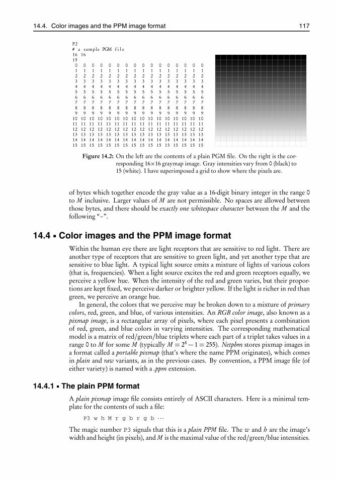
root2014/7/8page 117
�
�
�
�
�
�
�
�
14.4. Color images and the PPM image format 117
P2# a sample PGM f i l e16 1615
0 0 0 0 0 0 0 0 0 0 0 0 0 0 0 01 1 1 1 1 1 1 1 1 1 1 1 1 1 1 12 2 2 2 2 2 2 2 2 2 2 2 2 2 2 23 3 3 3 3 3 3 3 3 3 3 3 3 3 3 34 4 4 4 4 4 4 4 4 4 4 4 4 4 4 45 5 5 5 5 5 5 5 5 5 5 5 5 5 5 56 6 6 6 6 6 6 6 6 6 6 6 6 6 6 67 7 7 7 7 7 7 7 7 7 7 7 7 7 7 78 8 8 8 8 8 8 8 8 8 8 8 8 8 8 89 9 9 9 9 9 9 9 9 9 9 9 9 9 9 9
10 10 10 10 10 10 10 10 10 10 10 10 10 10 10 1011 11 11 11 11 11 11 11 11 11 11 11 11 11 11 1112 12 12 12 12 12 12 12 12 12 12 12 12 12 12 1213 13 13 13 13 13 13 13 13 13 13 13 13 13 13 1314 14 14 14 14 14 14 14 14 14 14 14 14 14 14 1415 15 15 15 15 15 15 15 15 15 15 15 15 15 15 15
Figure 14.2: On the left are the contents of a plain PGM file. On the right is the cor-responding 16×16 graymap image. Gray intensities vary from 0 (black) to15 (white). I have superimposed a grid to show where the pixels are.
of bytes which together encode the gray value as a 16-digit binary integer in the range 0to M inclusive. Larger values of M are not permissible. No spaces are allowed betweenthose bytes, and there should be exactly one whitespace character between the M and thefollowing “-”.
14.4 Color images and the PPM image formatWithin the human eye there are light receptors that are sensitive to red light. There areanother type of receptors that are sensitive to green light, and yet another type that aresensitive to blue light. A typical light source emits a mixture of lights of various colors(that is, frequencies). When a light source excites the red and green receptors equally, weperceive a yellow hue. When the intensity of the red and green varies, but their propor-tions are kept fixed, we perceive darker or brighter yellow. If the light is richer in red thangreen, we perceive an orange hue.
In general, the colors that we perceive may be broken down to a mixture of primarycolors, red, green, and blue, of various intensities. An RGB color image, also known as apixmap image, is a rectangular array of pixels, where each pixel presents a combinationof red, green, and blue colors in varying intensities. The corresponding mathematicalmodel is a matrix of red/green/blue triplets where each part of a triplet takes values in arange 0 to M for some M (typically M = 28− 1 = 255). Netpbm stores pixmap images ina format called a portable pixmap (that’s where the name PPM originates), which comesin plain and raw variants, as in the previous cases. By convention, a PPM image file (ofeither variety) is named with a .ppm extension.
14.4.1 The plain PPM format
A plain pixmap image file consists entirely of ASCII characters. Here is a minimal tem-plate for the contents of such a file:
P3 w h M r g b r g b · · ·The magic number P3 signals that this is a plain PPM file. The w and h are the image’swidth and height (in pixels), and M is the maximal value of the red/green/blue intensities.

root2014/7/8page 118
�
�
�
�
�
�
�
�
118 Chapter 14. Image I/O
P3# a sample PPM f i l e8 877 0 0 7 0 0 7 0 0 7 0 0 7 0 0 7 0 0 7 0 0 7 0 00 7 0 0 7 0 0 7 0 0 7 0 0 7 0 0 7 0 0 7 0 0 7 00 0 7 0 0 7 0 0 7 0 0 7 0 0 7 0 0 7 0 0 7 0 0 77 7 0 7 7 0 7 7 0 7 7 0 7 7 0 7 7 0 7 7 0 7 7 07 0 7 7 0 7 7 0 7 7 0 7 7 0 7 7 0 7 7 0 7 7 0 70 7 7 0 7 7 0 7 7 0 7 7 0 7 7 0 7 7 0 7 7 0 7 77 7 7 7 7 7 7 7 7 7 7 7 7 7 7 7 7 7 7 7 7 7 7 70 0 0 0 0 0 0 0 0 0 0 0 0 0 0 0 0 0 0 0 0 0 0 0 black
white
cyanmagentayellowblue
greenred
Figure 14.3: On the left are the contents of a PPM file. On the right is the corresponding8×8 pixmap image. I have superimposed a grid to show where the pixelsare. The RGB intensities vary from 0 (black) to 7 (full color). The matrixentries should be read three at a time. The first row consists of eight tripletsof the form {7 0 0}, which indicates that the top row of pixels are all red.The second row consists of eight triplets of the form {0 7 0}, whichindicates that the second row of pixels are all green.
They should be given as ordinary decimal numbers. The rest of the template consists ofa sequence of w× h of integer triplets, “r g b”, where each component is in the range 0to M inclusive, written as ordinary decimal numbers, with zero indicating an absolutelydim color (black) and M indicating the brightest possible color. What I have shown asspaces between the file’s entries can be one or more whitespaces of any kind, i.e., space,tab, newline, etc.; see Section 9.3.2 for the definition of “whitespace”. Additionally, a PPMfile may contain comments between P3 and w. A comment begins with a “#” characterand extends to the end of the line. Figure 14.3 shows the contents of a plain PPM file andthe corresponding 8×8 pixmap image. Here M is 7; therefore color intensities may rangefrom 0 to 7, although I have used only 0 and 7 in that sample.
14.4.2 The raw PPM format
The raw PPM format stores the pixmap image according to the template
P6 w h M ----- · · ·where the magic number P6 identifies the content as raw PPM, the w and h are imagewidth and height, and M is the upper range of color values, as before. If M < 28 = 256,then the rest of the file is a set of 3×w×h consecutive bytes. Each byte triplet encodes thered/green/blue colors of a pixel as three 8-digit binary numbers. If 28 ≤M < 216 = 65536,then rest of the file is a set of 6×w × h consecutive bytes. Each byte sextet encodes thered/green/blue colors of a pixel as three pairs of 16-digit binary numbers. Larger valuesof M are not permissible. Spaces and comments conform to the same requirements asthose of raw PGM files.
14.5 The libnetpbm libraryNetpbm’s libnetpbm library provides C functions for reading and writing PBM, PGM,and PPM images. The interface is declared in the header file pam.h, which declares a Cstructure called “struct pam” for storing all characteristics of an image other than itspixel values. Some of the structure’s members deal with issues outside the scope of thispresentation. Those members that are relevant to our work shown in Listing 14.1. Themeanings of the file, height, width members should be evident from the associated

root2014/7/8page 119
�
�
�
�
�
�
�
�
14.5. The libnetpbm library 119
Listing 14.1: A fragment of libnetpbm’s “struct pam” structure. Only those parts that are rele-vant to our work are shown.
1 typedef unsigned long sample;2 struct pam {3 ...4 FILE *file; // the image’s input or output stream5 int format; // coded value of image type6 int plainformat;// boolean: “true” if plain format, “false” if raw format7 int height; // image height, in pixels8 int width; // image width, in pixels9 int depth; // 1 for PBM and PGM, 3 for PPM
10 sample maxval; // same as M in the previous sections11 ...12 };
comments. The format member is an integer that encodes the image type. It is one ofPBM_FORMAT, PGM_FORMAT, PPM_FORMAT in the case of plain image formats or one ofRPBM_FORMAT, RPGM_FORMAT, RPPM_FORMAT in the case of raw image formats. Theplainformat member is a Boolean variable which is true (i.e., 1) if the image format isplain and false (i.e., 0) if the image format is raw. Considering that the format memberalready carries the information regarding raw versus plain, the plainformat memberappears to be redundant. In a sense, it is—it exists as a hack to address compatibility issueswith the earlier versions of libnetpbm. When writing an image to a file, the latest versionsof the library ignore the raw versus plain information contained in the format memberand use the raw format as a default. To get a plain format in the output, you will need toset plainformat to true.
The depth member is set to 1 for PBM and PGM images because these require asingle number to specify a pixel value. It is set to 3 for a PPM image because it requires3 numbers to specify a pixel value.
The maxval member is what I called M in the previous section. Pixel values areintegers in the range 0,1, . . . , M . The maxval is declared as an object of type “sample”.We see on line 1 that this is an alias for unsigned long in libnetpbm.
Libnetpbm provides a multitude of functions for manipulating image objects. In therest of this section I will describe those functions—10, to be precise—that we need in ourwork. The descriptions are terse but should be adequate for most purposes. For moredetails you should consult libnetpbm’s documentation.
void pm_init(const char *progname, unsigned int flags);
Every libnetpbm program should call pm_init() to initialize the library. The firstargument is the program’s name. The second argument is always zero. (It’s really a place-holder for possible future expansions of the library.)
FILE *pm_openr(char *name);FILE *pm_openw(char *name);FILE *pm_close(FILE *fp);
These are the fancy versions of the standard library’s fopen() and fclose() func-tions. Specifically, pm_openr() and pm_openw() open a file for reading or writing,respectively, and call exit() if something goes wrong. The file name "-" is interpretedas the stdin or stdout, as the case may be. The function pm_close() closes a previ-ously opened stream.

root2014/7/8page 120
�
�
�
�
�
�
�
�
120 Chapter 14. Image I/O
· · ·
g g g
a tuplerow of a PGM image
· · ·
R
G
B
R
G
B
R
G
B
a tuplerow of a PPM image
Figure 14.4: A tuplerow array holds the pixel data of one row of an image. The ar-ray’s length equals the image’s width. The array’s entries point to tuplevectors that hold a pixel’s gray values in the case of a PGM image (shownon the left) or the RGB values in the case of PPM image (shown on theright). The tuple vectors of a PGM image are of length 1. Those of aPPM image are of length 3.
void pnm_readpaminit(FILE *fp, struct pam *pam, int size);void pnm_writepaminit(struct pam *pam);
The function pnm_readpaminit() reads an image’s header information44 from thestreamfp and populates thepam structure with it. It expects to find the stream positionedat the start of the image’s header and leaves it positioned at the start of the image’s data.
The meaning of the size argument is a bit too complex to explain here, and probablyan explanation won’t be very illuminating. Suffice it to say that you should always passthe expression PAM_STRUCT_SIZE(tuple_type) for that argument. This assumesthat you have a relatively recent libnetpbm library. In the older versions of the library(specifically, versions before Netpbm 10.23) pass sizeof(struct pam) instead.
The function pnm_writepaminit() writes an image’s header, according to theinformation supplied in thepam structure, to the output stream associated with the image.
tuple *pnm_allocpamrow(struct pam *pam);void pnm_freepamrow(tuple *tuplerow);
These functions allocate and free memory for storing one row of an image’s pixel datainto an array called a tuplerow, shown schematically in Figure 14.4. The array’s lengthequals the image’s width. Each entry of the tuplerow is a pointer to an array, called atuple array. In the case of a PGM image, a tuple array has length 1. It holds the pixel’sgray value. In the case of a PPM image, a tuple array has length 3. It holds the pixel’sred, green, and blue values, in that order.
void pnm_readpamrow(struct pam *pam, tuple *tuplerow);void pnm_writepamrow(struct pam *pam, const tuple *tuplerow);
The function pnm_readpamrow() reads one row of an image into a tuplerowarray (see the previous paragraph). It expects to find the input stream associated with theimage to be positioned at the start of the desired row and leaves it positioned just after it.
The function pnm_writepamrow() writes one row of an image from a tuplerowarray. It expects to find the output stream associated with the image to be positionedwhere the row should start and leaves it positioned just after it.
44The image header is everything in the image file other than the pixel data section.
root2014/7/8page 121
�
�
�
�
�
�
�
�
14.7. The interface of the image-io module 121
14.6 A no-frills demo of libnetpbmThe file netpbm-minimal.c shown in Listing 14.2 provides a no-frills demo of libnetpbm.It reads a PGM image into a matrix a, draws a black line over it by changing the pixelsai i , i = 0,1,2, . . ., to zero, and then writes the result into another PGM file. If you haveread the descriptions of the libnetpbm functions in the previous section, you should haveno difficulty in following the program’s logic and understanding what it does; thereforeI will not elaborate on it any further other than pointing out that on line 42 we set the pamstructure’s plainformatmember to true or false, according to the input image’s format,so that a plain format input results in a plain format output and a raw format input resultsin a raw format output. In the absence of that line, the output image will be in the rawformat regardless of the input image’s format because that is libnetpbm’s default behavior.
The program depends on Chapter 8’s array.h, which in turn depends on Chapter 7’sxmalloc module. Therefore I suggest that you construct a Makefile according to the in-structions of Chapter 6 to build netpbm-minimal as well as the several other programswhich you will develop in this chapter. Here is the beginning part of the Makefile:
CFLAGS = -Wall -pedantic -std=c99 -O2LIBS = -lnetpbmnetpbm-minimal: xmalloc.o netpbm-minimal.o
$(CC) $^ $(LIBS) -o $@
14.7 The interface of the image-io moduleWe are going to develop an image-io module which will provide functions for readingand writing PGM and PPM images. Listing 14.3 shows the file image-io.h that pro-vides the module’s interface. It declares a “struct image”, which extends libnetpbm’s“struct pam” by adding new members r, g, b that point to h ×w matrices that holdan image’s red, green, and blue pixel values. (Here h and w are the image’s height andwidth in pixels.) Additionally, it declares the prototypes of functions that read and writeimages and free the allocated memory.
We use “struct image” with both PGM and PPM image types. In the case of aPGM image only one of the three matrix pointers r, g, b is needed. I will use theg pointerconsistently for that purpose since “g” may be thought of as standing both for “green” and“gray”. The r and b pointers are not used in that case and may be left unassigned.
Remark 14.4. Why are the r, g, b matrices in “struct image” of type double?The pixel values of an image are integers in the range 0 to M , where typically M is 28−1.Isn’t it more natural to store the numbers in a matrix of type unsigned char? Evenin the worst case, when M is 216−1= 65535), a matrix of type unsigned short intought to suffice.
Those observations are valid. Nevertheless, the type of storage for an image is dictatedby the application. I am using the type double for storage in anticipation of applicationsof the wavelet transform to image analysis, which is the subject of the next chapter. Therewe overwrite an image matrix with the corresponding wavelet transform, which is nolonger a matrix of integers. If your applications don’t do such drastic things to your im-ages, then feel free to change double to unsigned char or unsigned short intin image-io.h.
The image-io module relies on the xmalloc module (Chapter 7) for memory allocationand the array.h header file (Chapter 8) for building matrices. Therefore, following thesuggestions in Chapter 2, the project’s directory will contain

root2014/7/8page 122
�
�
�
�
�
�
�
�
122 Chapter 14. Image I/O
Listing 14.2: The file netpbm-minimal.c provides a no-frills demo of the libnetpbm functions.It reads a PGM image into a matrix, draws a black line over it, and then writesthe result into another PGM file. Calls to the libnetpbm functions are set on ashaded background .
1 #include <stdio.h>2 #include <pam.h>3 #include "array.h"4 int main(int argc, char **argv)5 {6 char *infile = "aya_matsuura.pgm";7 char *outfile = "zz.pgm";8 struct pam pam;9 FILE *fp;
10 double **a;11 tuple *row;12 int i, j;13
14 pm_init (argv[0], 0); // initialize the library15
16 // read image header17 fp = pm_openr (infile);
18 pnm_readpaminit (fp, &pam, PAM_STRUCT_SIZE(tuple_type));
19 printf("image: %dx%d, depth: %d\n",20 pam.width, pam.height, pam.depth);21 if (!(pam.format == PGM_FORMAT || pam.format == RPGM_FORMAT)) {22 fprintf(stderr, "Sorry, this demo handles PGM images only.\n");23 return EXIT_FAILURE;24 }25
26 make_matrix(a, pam.height, pam.width); // matrix to store image data27 row = pnm_allocpamrow (&pam); // tuplerow vector28 for(i = 0; i < pam.height; i++) { // read pixel data29 pnm_readpamrow (&pam, row);
30 for (j = 0; j < pam.width; j++) { // copy tuplerow into matrix31 a[i][j] = row [j][0];32 }33 }
34 pm_close (fp);
3536 for (i = 0; i < pam.width && i < pam.height; i++)
37 a[i][i] = 0.0; // change the ai i pixels to black38
39 // write image header40 fp = pm_openw (outfile);
41 pam.file = fp;42 pam.plainformat = pam.format == PGM_FORMAT ? 1 : 0;
43 pnm_writepaminit (&pam);
44
45 for (i = 0; i < pam.height; i++) { // write pixel data46 for(j = 0; j < pam.width; j++)47 row[j][0] = a[i][j];
48 pnm_writepamrow (&pam, row);
49 }
50 pm_close (fp);
51 free_matrix(a);
52 pnm_freepamrow (row);
53 return EXIT_SUCCESS;54 }

root2014/7/8page 123
�
�
�
�
�
�
�
�
14.7. The interface of the image-io module 123
Listing 14.3: The file image-io.h.
1 #ifndef H_IMAGE_IO_H2 #define H_IMAGE_IO_H3 #include <pam.h>4 struct image {5 struct pam pam;6 double **r;7 double **g;8 double **b;9 };
10 struct image *read_image(char *filename);11 void write_image(char *filename, struct image *img);12 void free_image(struct image *img);13 #endif /∗ H_IMAGE_IO_H */
$ cd image-io$ ls -FMakefile image-io-test-3.c netpbm-minimal.carray.h@ image-io-test-4.c [email protected] image-io-test-5.c [email protected] image-io.cimage-io-test-2.c image-io.h
The stand-alone file netpbm-minimal.c was presented in Section 14.6. The image-iomodule itself is contained in the files image-io.[ch]. The files image-io-test-[0–5].c are inde-pendent drivers for demonstrating the module’s functionality in various ways, as will bedescribed later. They compile to executables named image-io-test-[0–5]. Each executableis invoked with two arguments, as in
$ image-io-test-0 infile outfile
The program reads an image from infile, modifies the images in certain ways, and writesthe modified image to outfile. You may name the input and output files as you wish,but it is customary to name images in PGM and PPM formats with the .pgm and .ppmextensions, respectively. The program does not rely on a file name to determine the im-age format. Rather, it detects the image format through the magic number embedded inthe file.
Remark 14.5. In the descriptions of libnetpbm’s pm_openr() and pm_openw() func-tions in Section 14.5, we noted that these functions treat the special file name "-" as areference to the stdin or stdout. Therefore, the program may also be invoked as
$ image-io-test - outfile.pgm <infile.pgm
or even as
$ image-io-test - - <infile.pgm >outfile.pgm
These will work in Unix or in Unix-like systems where a file is treated a stream of bytes.On an operating system such as Windows that distinguishes between text and binary files,the redirection may corrupt a raw image.
root2014/7/8page 124
�
�
�
�
�
�
�
�
124 Chapter 14. Image I/O
Listing 14.4: An outline of the file image-io.c.
1 #include <stdio.h>2 #include <stdlib.h>3 #include "array.h"4 #include "image-io.h"5 � static void read_pgm_pixel_data(struct image *img) ...6 � static void read_ppm_pixel_data(struct image *img) ...7 � struct image *read_image(char *filename) ...8 � static void write_pgm_pixel_data(struct image *img) ...9 � static void write_ppm_pixel_data(struct image *img) ...
10 � void write_image(char *filename, struct image *img) ...11 � void free_image(struct image *img) ...
Listing 14.5: An implementation of the function read_image().
1 struct image *read_image(char *filename)2 {3 struct image *img = xmalloc(sizeof *img);4 struct pam *pam = &img→pam;5 FILE *fp = pm_openr(filename);6 pnm_readpaminit(fp, pam, PAM_STRUCT_SIZE(tuple_type));7 if (pam→format == PGM_FORMAT || pam→format == RPGM_FORMAT)8 read_pgm_pixel_data(img);9 else if (pam→format == PPM_FORMAT || pam→format == RPPM_FORMAT)
10 read_ppm_pixel_data(img);11 else {12 fprintf(stderr, "error: file ‘%s’ contains neither "13 "a PGM nor a PPM image\n", filename);14 exit(EXIT_FAILURE);15 }16 pm_close(fp);17 return img;18 }
14.8 The implementation of the image-io moduleListing 14.4 shows an outline of the file image-io.c. I will give the details of the partsdealing with PGM images. You will write the parts dealing with PPM images.
14.8.1 The function read_image()
The function read_image() that appears on line 7 of Listing 14.4 receives the name ofan existing image file. It reads the file’s contents, allocates memory for a “struct image”structure and its members, populates the structure with the image’s data, and returns apointer to that structure. If anything fails in the process, it prints a diagnostic message tothe stderr and calls exit() to kill the program. Listing 14.5 shows my implementa-tion of read_pgm_image(). It handles PGM and PPM images, both the plain and rawtypes. Extending it to handle PBM images is straightforward, and you are welcome to tryit yourself, but I will refrain from doing so in the interest of brevity.

root2014/7/8page 125
�
�
�
�
�
�
�
�
14.8. The implementation of the image-io module 125
Let us go through the details of the function read_image().
Line 3. We allocate memory for a “struct image” and set img to point to that mem-ory location. The purpose of the current function is to read image data from theinput file, deposit that information into that structure, and return the structure’saddress to the caller.
Line 4. The pointer &img→pam is needed in quite a few places in the rest of the code. Itwouldn’t be wrong to write &img→pam everywhere, but it would clutter things.The pam variable defined here is a shorthand meant to reduce clutter; doing so isn’tessential in any way.
Line 5. Here we call libnetpbm’s pm_openr() function, described in Section 14.5, toopen the image file for reading. We could have called C’s standard fopen() in-stead, as in
FILE *fp = fopen(filename, "r");
but, as noted in Section 14.5, pm_openr() offers a couple of extra helpful features.For one thing, it treats the file name "-" as a request for stdin, as seen in the usageexamples in Remark 14.5 on page 123. For another thing, it checks for errors. Ifthe requested file cannot be opened for reading, it prints a message to stderr andexits the program! Consequently, there is no point in checking for the success ofthe pm_openr() call.
Line 6. Here we call libnetpbm’s pnm_readpaminit() function, described in Sec-tion 14.5, to read the image’s header data. The first argument is the stream fp,which was set up on the previous line. The second argument, pam, points to the“struct pam”, which is embedded in “struct image”. The function willpopulate pam’s members (see Listing 14.1) with the information that it extractsfrom the image’s header. The third argument, as noted in Section 14.5, is alwaysthe expression I have shown. Also as was noted there, you may have to change it tosizeof(struct pam) if you have an older version of libnetpbm.
Line 7. Here the program branches depending on the image type. The format memberof “struct pam” encodes the image type that has just been read from the inputstream (see Section 14.5 for the details of the “struct pam”). If the image is oftype PGM, we callread_pgm_pixel_data() to read the pixel data. If the imageis of type PPM, we call read_ppm_pixel_data() to read the pixel data. (Thesefunctions will be described shortly.) If the image is something else—presumably aPBM or a PAM45—then we print a message saying that we are not prepared to handlethat type and exit the program.
Lines 16 and 17. We are done with reading the image; therefore we close the input streamand returnimg to the caller. The functionpm_close(), described in Section 14.5,is a wrapper around C’s standard fclose()—it checks for fclose()’s returnstatus and calls exit() if an error occurs.
45I have neither mentioned the PAM format up to this point, nor will I deal with it from here on. PAM isan “adaptable” format in the sense that any PBM, PGM, or PPM image may be presented as a PAM image. Youwill have to read Netpbm’s documentation if you want to learn more about that format.

root2014/7/8page 126
�
�
�
�
�
�
�
�
126 Chapter 14. Image I/O
Listing 14.6: The implementation of the function read_pgm_pixel_data().
1 static void read_pgm_pixel_data(struct image *img)2 {3 struct pam *pam = &img→pam;4 tuple *row = pnm_allocpamrow(pam);5 make_matrix(img→g, pam→height, pam→width);6 img→r = img→b = NULL;7 for (int i = 0; i < pam→height; i++) {8 pnm_readpamrow(pam, row);9 for (int j = 0; j < pam→width; j++)
10 img→g[i][j] = row[j][0];11 }12 pnm_freepamrow(row);13 }
14.8.2 The function read_pgm_pixel_data()
The function read_pgm_pixel_data() that appears on line 5 of Listing 14.4 readsthe pixel data of a PGM image. Its implementation is shown in Listing 14.6. Let us gothrough the details.
Line 3. The variable pam is introduced here for the same reason as that on line 4 of List-ing 14.5. It’s not essential in any way; it’s a shorthand meant to reduce clutter.
Line 4. Here we call libnetpbm’s pnm_allocpamrow() function, described in Sec-tion 14.5, to allocate memory for a tuplerow array. We are going to read theimage one row at a time into that array and then copy the result into a matrix. Fig-ure 14.4 shows a schematic representation of a tuplerow array. There is no needto check for success—if memory allocation fails, pnm_allocpamrow()will printa message to stderr and exit the program.
Lines 5 and 6. We call the make_matrix() macro from the header file array.h (seeChapter 8) to allocate a matrix of double, assigned to img→g, to hold the pixeldata of a (pam→height) × (pam→width) image. The members img→r andimg→b are meant for use in PPM images, so they are not needed here. We setthem to NULL so that they can be passed to free_matrix() with no ill effects;see subsection 14.8.5.
Lines 7–11. The for-loop goes through the image one row at a time. At each step it callslibnetpbm’s pnm_readpamrow() function, described in Section 14.5, to read anentire row into therow array. Thus, row[j] points to the tuple associated with thepixel at rowi and columnj. Since this is a PGM image, the tuple vector has length 1(see Figure 14.4); therefore its first (and only) element is given by row[j][0]. Westore that value in img→g[i][j].
Line 12. We are done with reading. We call libnetpbm’s pnm_freepamrow() function,described in Section 14.5, to free the memory allocated on line 4.
14.8.3 The function write_image()
The function write_image() that appears on line 10 of Listing 14.4 receives the nameof an output file and a pointer to a fully populated “struct image”. It writes the

root2014/7/8page 127
�
�
�
�
�
�
�
�
14.8. The implementation of the image-io module 127
Listing 14.7: The implementation of the function write_image().
1 void write_image(char *filename, struct image *img)2 {3 struct pam *pam = &img→pam;4 pam→file = pm_openw(filename);5 pam→plainformat6 = (pam→format == PGM_FORMAT || pam→format == PPM_FORMAT) ? 1 : 0;7 pnm_writepaminit(pam);8 if (pam→format == PGM_FORMAT || pam→format == RPGM_FORMAT)9 write_pgm_pixel_data(img);
10 else if (pam→format == PPM_FORMAT || pam→format == RPPM_FORMAT)11 write_ppm_pixel_data(img);12 else {13 fprintf(stderr, "error: file %s, line %d: shouldn’t be here!\n",14 __FILE__, __LINE__);15 exit(EXIT_FAILURE);16 }17 pm_close(pam→file);18 }
image’s data into the named file as a PGM or PPM image. If a file of the given namedoes not exist, it’s created. If it exists, it’s overwritten. If anything fails in the process, itprints a diagnostic message to the stderr and exits the program. Listing 14.7 shows theimplementation of write_image().
Line 3. We introduce the variable pam as a shorthand for &img→pam, just as we did inread_image(). This is not essential; it serves only to reduce clutter.
Line 4. Here we call libnetpbm’s pm_openw() function, described in Section 14.5, toopen the image file for writing. We could have called C’s standard fopen() in-stead, as in
FILE *fp = fopen(filename, "w");
but, as noted in Section 14.5, pm_openw() offers a couple of extra helpful features.For one thing, it treats a file named "-" as a request for stdout; see the usageexamples in Remark 14.5 on page 123. For another thing, it checks for errors. Ifthe requested file cannot be opened for writing, it prints a message to stderr andexits the program! Consequently, there is no point in checking for the success ofthe pm_openw() call.
Note that we set pam→file to the stream opened by pm_openw(). Other func-tions which write to the stream look up the stream’s address in the pam structure.
Line 5. As noted in Section 14.5, libnetpbm ignores the format encoded in the pam struc-ture’s formatmember and writes images in the raw format by default. Here we ex-amine theformatmember. If it indicates a plain format, we set theplainformatmember to true to override the library’s default behavior.
Line 7. Libnetpbm’spnm_writepaminit() function, described in Section 14.5, writesan image’s header data (e.g., the “P5 w h M” part described in subsection 14.3.2)by extracting the needed information from the pam structure. The output goes tothe stream pam→file.

root2014/7/8page 128
�
�
�
�
�
�
�
�
128 Chapter 14. Image I/O
Listing 14.8: The implementation of the function write_pgm_pixel_data().
1 static void write_pgm_pixel_data(struct image *img)2 {3 struct pam *pam = &img→pam;4 tuple *row = pnm_allocpamrow(pam);5 for (int i = 0; i < pam→height; i++) {6 for (int j = 0; j < pam→width; j++)7 row[j][0] = img→g[i][j];8 pnm_writepamrow(pam, row);9 }
10 pnm_freepamrow(row);11 }
Line 8. Here the program branches depending on the image type. If the image is of typePGM, we call write_pgm_pixel_data() to write the pixel data. If the im-age is of type PPM, we call write_ppm_pixel_data() to write the pixel data.(These functions will be described shortly.) Unless we have carelessly meddled withthe pam structure’s format member, these two should be the only possibilities.Anything else is abnormal and should never occur. Nevertheless, we supply codeto catch the hypothetical implausible case, write a diagnostic, and exit the program.
Line 17. We are done with writing; therefore we call pm_close(), described in Sec-tion 14.5, to close the output stream. The function pm_close() is a wrapperaround C’s standard fclose()—it checks for fclose()’s return status and callsexit() if an error occurs.
14.8.4 The function write_pgm_pixel_data()
The function write_pgm_pixel_data() that appears on line 8 of Listing 14.4 hasmany aspects in common with read_pgm_pixel_data(); therefore my commentswill be somewhat terser here. It receives a pointer to a fully populated “struct image”corresponding to a PGM image and writes the image’s pixel data into an output stream.Its implementation is shown in Listing 14.8. Let us go through the details.
Lines 3 and 4. These are just like what we had in read_pgm_pixel_data(). Readthe explanations there.
Lines 5–9. The outer for-loop goes through the img→g matrix one row at a time.The inner for-loop goes through the row and copies the value of img[i][j]to the first (and only) element of the tuple associated with the pixel row[j]. (Thisis the opposite of what we did when reading the image.)
Remark 14.6. Note that img→g[i][j] is of type double, while row[j][0]is of type “sample”, which is an alias for unsigned long. C’s automatic con-version rules are applied during the assignment. If the right-hand side is an integerstored as a double, then the left-hand side receives the exact value of that integer. Ifthe right-hand side is a noninteger, then its fractional part is dropped! For instance,both 3.1 and 3.9 are converted to 3; no rounding takes place. It is the responsibilityof the caller to do all necessary rounding/processing on the image’s sample valuesbefore arriving here. In particular, it is the caller’s responsibility to ensure that the

root2014/7/8page 129
�
�
�
�
�
�
�
�
14.9. The file image-io-test-0.c 129
Listing 14.9: The implementation of free_image() in file image-io.c.
1 void free_image(struct image *img)2 {3 if (img �= NULL) {4 free_matrix(img→r);5 free_matrix(img→g);6 free_matrix(img→b);7 free(img);8 }9 }
sample values lie in the range 0 to M , where M is the image’s maximum samplevalue. In Chapter 15’s applications of wavelets to image analysis, we take care ofthese details before write_pgm_pixel_data() is called. This is the purpose ofthe clip_matrx() function introduced in subsection 15.6.2.
Line 8. The function pnm_writepamrow(), described in Section 14.5, writes the pixeldata for an entire row of an image to the output stream.
Line 10. Here we free the memory associated with the row vector which was previouslyallocated on line 4.
14.8.5 The function free_image()
The function free_image() that appears on line 11 of Listing 14.4 (page 124) freesmemory resources associated with a “struct image”. The implementation shown inListing 14.9 is quite straightforward. It frees the following:
• The memory associated with the matrices img→r, img→g, img→b, allocated inread_pgm_pixel_data() or read_ppm_pixel_data(); see line 5 of List-ing 14.6 on page 126.
• The memory associated with the img structure, allocated in readimage(); seeline 3 of Listing 14.5 on page 124.
As with all other free_*() functions in this book, as well as the standard library’sfree(), calling free_image() with a NULL argument is safe.
Remark 14.7. Note the significance of NULL-ing the img→r and img→b pointers online 6 in Listing 14.6. Our free_matrix() in array.h is implemented to handle a NULLargument gracefully.
14.9 The file image-io-test-0.cThe file image-io-test-0.c, shown in Listing 14.10, provides a driver for exercising the image-io module. It simply reads a PGM or PPM image (plain or raw format) and writes it outwithout change, except for embedded comments, if any, which are discarded. The namesof the input and output files are obtained from argv[1] and argv[2]. Thus, it isinvoked as
$ image-io-test-0 infile outfile

root2014/7/8page 130
�
�
�
�
�
�
�
�
130 Chapter 14. Image I/O
Listing 14.10: The file image-io-test-0.c, shown in its entirety here, provides a driver for exercisingthe image-io module. It reads a PGM or PPM file and writes it out without change,except for embedded comments, if any, which are discarded. The names of the inputand output files are obtained from argv[1] and argv[2].
1 #include <stdio.h>2 #include "image-io.h"3 int main(int argc, char **argv)4 {5 if (argc �= 3) {6 fprintf(stderr, "Usage: %s infile outfile\n", argv[0]);7 fprintf(stderr, "Reads PGM or PPM from infile, "8 "writes identical image to outfile\n");9 return EXIT_FAILURE;
10 }11 pm_init(argv[0], 0);12 struct image *img = read_image(argv[1]);13 fprintf(stderr, "image is %dx%d, depth=%d, maxval=%d\n",14 img→pam.height, img→pam.width,15 img→pam.depth, (int)img→pam.maxval);16 write_image(argv[2], img);17 free_image(img);18 return EXIT_SUCCESS;19 }
See Section 14.7 regarding the invocation details. Here is a line-by-line description ofimage-io-test-0.c:
Line 5. We expect the program to be invoked with exactly two arguments, Thus, argcshould be 3 (see Section 4.7). Then argv[0] is the program’s name, argv[1] isthe name of the input image file, and argv[2] is the name of the output image file.If argc is other than 3, we print a message to stderr and exit.
Line 11. As noted in Section 14.5, every libnetpbm program is expected to callpm_init()to initialize the library. The first argument of pm_init() should be the name ofthe program. The second argument is always zero.
Line 12. The function read_image() (see subsection 14.8.1) reads the image file cor-responding to argv[1]. When it returns, everything about the image is stored inthe img structure.
Note the midblock declaration of struct image. This is permissible in C99but not in C89. If you wish to reduce the code to C89, then insert a declarationstruct image *img; at the top of the block and change the current line toimg = read_image(argv[1]);.
Line 13. We print some of the image’s data as a feedback to the user. The value of depthwill be 1 in the case of a PGM image and 3 in the case of a PPM image.
Line 16. The function write_image() (see subsection 14.8.3) writes the image fromthe img structure into the file corresponding to argv[2].
Line 17. We call the function free_image() (see subsection 14.8.5) to free all memoryresources associated with the image and then exit.
root2014/7/8page 131
�
�
�
�
�
�
�
�
14.10. Project Image I/O 131
14.10 Project Image I/O
Part 14.1. Complete, compile, and test the netpbm-minimal program of Section 14.6.
Part 14.2. In the preceding sections I gave the complete code for reading and writingPGM images. Complete the image-io module by adding functionality to handle PPMimages. This requires implementing the functions read_ppm_pixel_data() andwrite_ppm_pixel_data(); see lines 6 and 9 of Listing 14.4 on page 124. Modifi-cations relative to the PGM image handling code are very slight. Figure 14.4 on page 120should provide all the hints you need to get started.
Part 14.3. Compile and test your image-io-test-0 using some of the PGM and PPM imagesthat I have provided in the book’s website.46 For instance,
$ ./image-io-test-0 aya_matsuura.pgm z0.pgmimage is 512x512, depth=1, maxval=255
The program reads the image file aya_matsuura.pgm and writes the new image file z0.pgm.Since we have not modified the image, the two files should be identical. You may applythe Unix utility called cmp to verify that the files are indeed identical:
$ cmp aya_matsuura.pgm z0.pgm
If the files being compared are different, cmp prints the location of the first byte where adifference occurs. If the files are identical, cmp exists silently.
Remark 14.8. It is not true in general that the input and output files of image-io-test-0will be identical. In the description of image file formats—see, e.g., subsection 14.3.2—Inoted that an image’s header material may be interspersed with optional comments andwhitespace. Our read_image() function discards header comments as they are read.Therefore two identical images need not have identical files since their header sections maybe different. Nevertheless, the image files in the book’s website contain no comments (ex-cept for the one noted explicitly as such), and the whitespace in their headers is accordingto what libnetpbm’s utilities create; therefore your aya_matsuura.pgm and z0.pgm shouldbe identical. If not, your program is buggy.
Part 14.4. [optional]Write a program file, image-io-test-1.c, that converts a (color) PPMimage to a (grayscale) PGM image. I suggest that you start with a copy of image-io-test-0.c shown in Listing 14.10. Between reading the image (line 12) and writing the image(line 16) insert
img→pam.format = RPGM_FORMAT;img→pam.depth = 1;
This sets the image’s output format to raw PGM and the image’s depth to 1 because aPGM image’s pixel values are identified by a single number. Now, loop over the image,and at each pixel do
double avg = (img→r[i][j] + img→g[i][j] + img→b[i][j])/3.0;img→g[i][j] = (int)(0.5 + avg);
On the first line, we compute the average of the pixel’s red, green, and blue values. Theaverage is not necessarily an integer; however, a PGM image expects integers for its pixel
46See Remark 14.3 on page 114.

root2014/7/8page 132
�
�
�
�
�
�
�
�
132 Chapter 14. Image I/O
values. Therefore, on the second line we cast the result to an int before assigning it toimg→g[i][j]. Note that casting a double to int discards the number’s fractionalpart. Adding the 0.5 ensures proper rounding. For instance, if avg is 3.1, then 0.5+ 3.1is 3.6, which, after discarding the fractional part, is reduced to 3. On the other hand, ifavg is 3.9, then 0.5+ 3.9 is 4.4, which, after discarding the fractional part, results in 4.You will find an extended discussion of this in subsection 15.6.2 on page 141.
Your program will expect to be invoked with two arguments, as in
$ ./image-io-test-1 infile outfile
where infile is expected to be a PPM image. It should complain if it is invoked withthe wrong number of arguments or if the infile is not a PPM image. Here is what minedoes:
# invoked with too few args$ ./image-io-test-1Usage: ./image-io-test-1 infile outfileReads PPM image from infile, writes averaged PGM image to outfile
# infile is not a PPM image$ ./image-io-test-1 aya_matsuura.pgm z1.pgm./image-io-test-1: expected a PPM image in input
# a normal run$ ./image-io-test-1 aya_matsuura.ppm z1.pgminput image is 512x512, depth=3, maxval=255
Part 14.5. [optional] As natural as the straight averaging of the RGB values may seem,it does not work quite well. The fact is, the human eye is not equally sensitive to theluminosity of the red, green, and blue colors. Experience shows that a weighted average,with a larger weight attached to the green component, produces more natural-lookingresults. Libnetpbm’s conversion routines mix the red, green, and blue in the 77 : 150 : 29proportions, although this is not a hard and fast rule.
Copy image-io-test-1.c to image-io-test-2.c, and, noting that 77+150+29= 256, changethe averaging formula to
double avg = (77*img→r[i][j] + 150*img→g[i][j]+ 29*img→b[i][j])/256.0;
Apply the program to convert the previous PPM image into a file z2.pgm. View andcompare the images z1.pgm and z2.pgm.
Part 14.6. [optional] The image viewing program Xv averages the red, green, and bluecolors in the 20:32:12 proportions. Copy image-io-test-2.c to image-io-test-3.c, and changethe averaging algorithm according to this. Apply the program to convert the previousPPM image into a file z3.pgm. View and compare the images z1.pgm, z2.pgm, and z3.pgm.
Part 14.7. [optional] Copy image-io-test-0.c to image-io-test-4.c. Modify it so that it “ro-tates” the colors of a PPM image. That is, it writes the red colors to the green matrix, thegreen colors to the blue matrix, and the blue colors to the red matrix. View the resultingimage.
Part 14.8. [optional]Write a program file, image-io-test-5.c, that draws a black “X” overan image’s diagonals. In an image of height h and width w, the diagonal D1 that goes from

root2014/7/8page 133
�
�
�
�
�
�
�
�
14.10. Project Image I/O 133
the northwest to the southeast is given by
D1 = {(i , j ) : i = 0, . . . , h − 1, j = i(w − 1)/(h − 1)}.Observe that when i = 0, we get j = 0, and when i = h − 1, we get j = w − 1, asexpected. Note, however, that since i , h, and w are integers, the proper C encoding of theformula is
int j = 0.5 + (double)i*(w-1)/(h-1);
You figure out how to do the other diagonal. See Part 14.4 for an explanation of theextra 0.5.

root2014/7/8page 135
�
�
�
�
�
�
�
�
Chapter 15
Image analysis
Prerequisites: Chapters 7, 8, 13, 14
15.1 IntroductionIn Chapter 14 we saw how to import a PGM or PPM image as a matrix of pixels. InChapter 13 we saw how to apply the Haar wavelet transform to express a matrix in termsof the Haar wavelet basis. In this chapter we bring these techniques to their natural con-clusion by applying the Haar wavelet transform to an image. This decomposes the imageinto a sum of progressively finer wavelets. The very fine wavelets tend to have very smallcoefficients because they measure the differences between the image’s nearby pixels. Inan ordinary photograph, say of a person’s face, the differences between adjacent pixels aresmall, in general, because the texture and coloration vary smoothly. The cheeks, chin,and the forehead tend to be wide expanses of slowly varying pixels. There are exceptions,however. For instance, a finely knitted sweater, or distinctively combed hair, may exhibitsignificant variations even at the pixel scale. In any case, even in images containing finetextures, most of the coefficients of the finer wavelets tend to be very small. Figure 15.1shows a 512×512 grayscale image47 on the right. The two graphs on the left show the ab-solute values of the image’s wavelet coefficients, sorted in decreasing order in size. Thus,the horizontal axis enumerates the coefficients (these go from 1 to 512× 512 = 262,144)and the vertical axis is their magnitudes. The graph on the top shows the full range of theover quarter million coefficients. You can hardly see anything there because essentiallyall the coefficients are practically zero, and thus the graph coincides with the horizontalaxis. If you look very closely, you may discern a slight rounding near the origin. That’sall there is to be seen of the graph. In the bottom graph I have expanded the horizontalrange 1, . . . , 80 of the upper graph to zoom into the details near the origin. The very firstcoefficient is approximately 115. The next few are approximately 42, 41, 21, 16, 14, andthey drop rapidly after that.
This raises an intriguing question: What if we keep the first few thousand significantwavelet coefficients and discard the rest? Reconstructing the image from the retained co-efficients should yield a relatively faithful representation of the image since the discardedones are too small to matter.
47Actually the image that you see in the book has been reduced to fit the page. The actual image I analyzedwas 512× 512.
135

root2014/7/8page 136
�
�
�
�
�
�
�
�
136 Chapter 15. Image analysis
Figure 15.1: On the right we see a 512× 512 grayscale image. The graphs on the leftshow the absolute values of the image’s Haar wavelet coefficients, sortedin decreasing order in size. The upper graph shows all of the 512× 512=262,144 coefficients, while the lower graph zooms into the first 80. Thereis hardly anything visible in the upper graph because the points mostlycoincide with the coordinate axes. In the zoomed lower graph we see thelargest coefficient, which is approximately 115, as an isolated dot at the topof the vertical axis. The next few coefficients are approximately 42, 41, 21,16, and 14. Photograph courtesy of Stockvault.
It is this chapter’s objective to investigate that question. Experimenting with close-upimages of human faces, we find out that retaining around 5 percent of the largest waveletcoefficients suffices to recreate an image which is hardly distinguishable from the original.This observation has practical implications. For one thing, we may save a good deal ofstorage space by storing a small fraction of the wavelet coefficients instead of a full image.More importantly, if we are willing to accept a slightly deteriorated image, we may savesubstantially in network transmission time and broadcast bandwidth if we send only thesignificant wavelet coefficients. All that is needed is a Haar wavelet transformation andtruncation at the sending end and an inverse Haar wavelet transformation at the receivingend. Most videos that you watch on the Internet are brought to you this way.
This chapter’s program reads a PGM or PPM image, applies the Haar wavelet trans-form to it, and then discards as many of the smallest wavelet coefficients as possible, whilekeeping the truncation error below a prescribed threshold. It then reconstructs the im-age from the remaining wavelets and writes it out to a file. Since the wavelet techniquesthat we developed in Chapter 13 work with matrices whose dimensions are powers of 2,this chapter’s program handles images whose dimensions are powers of 2. Images of arbi-trary sizes may be cropped or padded to make them conform to this requirement.
Remark 15.1. The word “discard” can be somewhat ambiguous in this context, so letme clarify. By “discarding a coefficient” I mean setting it to zero. Afterward, when theimage is reconstructed as a sum of the products of the coefficients and the correspond-ing wavelets, a zeroed coefficient does not contribute to the sum; therefore in effect it is“discarded”.
Remark 15.2. Applying the wavelet transform to an image’s matrix and discardingthe small entries leaves us with a sparse matrix, that is, a matrix whose vast majority of

root2014/7/8page 137
�
�
�
�
�
�
�
�
15.2. The truncation error in a grayscale image 137
entries are zero. The sparse matrix storage techniques of Chapter 11 may be applied quiteprofitably here to store such transformed and truncated images, but I will not pursue thatissue here. You may find it instructive to explore the idea on your own.
15.2 The truncation error in a grayscale imageWe saw in Chapter 13 that the wavelet bases are orthonormal sets; therefore, if a = (ai j )
are the entries of a grayscale image’s wavelet coefficients, then ‖a‖ = �∑i , j a2
i j
1/2 is anorm on the space of grayscale images. The absolute error after dropping all coefficientsbelow a threshold t is eabs(t ) =
�∑|ai j |≤t a2
i j
1/2. The numerical value of the absolute errorby itself, however, is not of much interest. The relative error erel(t ) = eabs(t )/‖a‖ is muchmore illuminating since it puts the size of the truncation error in context. The relativeerror is a number between 0 and 1.
Our program receives a grayscale image and a user-specified relative error erel in theinterval [0,1]. It proceeds to determine the cut-off threshold t so that erel( t ) = erel, orequivalently,
eabs( t ) = ‖a‖erel.
The most obvious way of finding t is through the bisection algorithm (or bisection method;see, e.g., [4, 33]). Here is how:
1. Sweep through the matrix a to find the largest and smallest values of |ai j |. Call themmax and min. While you are at it, also compute ‖a‖.
2. The cut-off threshold t lies somewhere in the interval [min,max]. As an initialguess, pick t at the midpoint, that is, t = (max+min)/2.
3. Evaluate the truncation error eabs(t ) =�∑
|ai j |≤t a2i j
1/2 corresponding to that cut-off value.
4. There are three cases:
(a) Case eabs(t ) = ‖a‖erel: We have found just the right t . Stop.(b) Case eabs(t ) > ‖a‖erel: We are truncating too much. Set max = t , and go to
step 2.(c) Case eabs(t ) < ‖a‖erel: We are truncating too little. Set min = t , and go to
step 2.
In each iteration step, the length of the search interval is cut in half; therefore the iterationwill converge in a few steps. Or will it?
Unfortunately, chances are excellent that the iteration described above never will ter-minate. The problem lies in the stopping criterion in step 4(a). Actually there are twoproblems with that step. First, a comparison of floating point numbers for equalityis inherently problematic since most numbers have no exact representation as floatingnumbers. A minuscule floating point rounding here and there may throw off the equal-ity. Second, even in the absence of floating point rounding, we don’t expect the equalityeabs(t ) = ‖a‖erel ever to be satisfied in general. The eabs(t ) is computed as a discrete sum ofterms. Adding or taking away an extra term is likely to move the sum from just below‖a‖erel to just above it. There may be no combination of ai j terms that hits the targetexactly.
The way to fix things is to change the stopping criterion in step 4(a) to somethingwith more certainty. We know that the length of the search interval is halved in every

root2014/7/8page 138
�
�
�
�
�
�
�
�
138 Chapter 15. Image analysis
step, so let’s stop if that length is smaller than a small fraction of the image’s norm, as inmax−min < ε‖a‖, and set ε arbitrarily to something small, like 10−6. In summary, wechange the stopping condition in step 4(a) to
4(a)’: Stop if max−min< ε‖a‖.Remark 15.3. Although the definitions of the norm and the absolute error involvesquare roots, there is no need for computing square roots at all in the algorithm describedabove. For instance, the condition eabs(t ) > ‖a‖erel is equivalent to eabs(t )
2 > ‖a‖2 e2rel,
which involves no square roots.
15.3 The truncation error in a color imageIn Chapter 14 we encoded a PPM image as a superposition of three matrices of the image’sred, green, and blue intensities. Therefore we may apply the Haar wavelet transformto each of the three matrices, truncate them in conformance to the prescribed relativeerror erel, and then reconstruct the approximate image from the set of remaining waveletcoefficients. In that respect, color images offer no new challenges. There is a subtle issueto account for, however.
Truncating the three color matrices independently of each other can distort the im-age’s color balance. This is because a pixel’s blue component, for instance, may be elim-inated while its red component survives. To remain faithful to the original colors, weshould change a pixel’s RGB colors in unison. Here is what I suggest. Let ri j , gi j , bi j bethe entries of the (wavelet transformed) red, green, and blue matrices. Create a compositematrix, let’s call it T , such that T 2
i j =13 (r
2i j + g 2
i j +b 2i j ). That is, Ti j is the root mean square
of ri j , gi j , bi j . Truncate the matrix T in conformance to the prescribed relative error erel,just as if it represented a grayscale image. For any Ti j that gets dropped in the process,drop all three of the corresponding ri j , gi j , bi j entries.
15.4 Image reconstructionAt this point we have discarded an image’s wavelet coefficients that fall below a certainthreshold. Now we apply the inverse wavelet transform to the truncated coefficients toconstruct an approximation to the original image.
There is a slight complication here that requires our attention. Let’s say that the orig-inal image’s pixel values (color or grayscale) range from 0 to M . If we apply the wavelettransform to the image, followed by the inverse wavelet transform, without modifyinganything in between, the reconstructed image will be identical to the original, and ofcourse the reconstructed pixel values will be integers in the 0 to M range. However, if wemodify the transformed matrix, as we do when we discard some of its coefficients, thereis no guarantee that the pixel values of the reconstructed image will be integers, nor thatthey will fall in the 0 to M range. The result would be an illegal PGM or PPM image ingeneral.
In practice, we find that only a handful of the hundreds of thousands of pixel valuesfall outside the 0 to M range. We treat them by brute force. If a pixel value has fallenbelow zero, we set it to zero. If it exceeds M , we set it to M . If it is not an integer,we round it to the nearest integer. These are done in the clip_matrix() function insubsection 15.6.2.

root2014/7/8page 139
�
�
�
�
�
�
�
�
15.5. The program 139
Listing 15.1: The transcript of an interactive session with this chapter’s program. If invoked withtoo few or improper arguments, it prints a usage message to stderr and exits. Theimage file profile.pgm is available at the book’s website.
$ ./image-analysisUsage: ./image-analysis rel_err infile outfile
0.0 ≤ rel_err ≤ 1.01. Reads a PGM or PPM image from infile2. Applies the Haar wavelet transform3. Sets as many of the smallest wavelet coefficients to zero
as possible while keeping the relative error(in the L^2 norm) just under rel_err
4. Reconstructs image with the truncated coefficients andwrites to outfile
$ ./image-analysis 0.05 profile.pgm profile-05.pgmzeroed 258548 of 262144 wavelet coefficients, 3596 remaining
15.5 The programThis chapter’s program relies on the image-io module (Chapter 14) for reading and writingimages, the wavelet module (Chapter 13) for the Haar wavelet transform, the xmallocmodule (Chapter 7) for memory allocation, and the array.h header file (Chapter 8) formaking vectors and matrices. Therefore, following the suggestions in Chapters 2 and 6,this project’s directory will look like this:
$ cd image-analysis$ ls -FMakefile image-analysis.c image-io.h@ wavelet.h@ [email protected]@ image-io.c@ wavelet.c@ xmalloc.c@
The program is contained entirely in the file image-analysis.c, to be detailed below, andcompiles into an executable named image-analysis. It is expected to be invoked as in
$ ./image-analysis 0.12 infile outfile
The infile is the name of an existing PGM or PPM file; the 0.12 says that we want totruncate the image’s wavelet coefficients with a relative error of 0.12, that is, 12 percent.The program does that, constructs an image with the truncated coefficients, and writesit into the file outfile. The file names can be anything, but beware that the output willoverwrite a file with the same name as the outfile, if one exists. The relative error canbe anything from 0.0 to 1.0.
Listing 15.1 shows the transcript of an interactive session. If the program is invokedwith too few or improper arguments, it prints a usage message to stderr and exits. Oth-erwise it does what is expected of it and prints out a brief statistics regarding its operation.
15.6 The implementation of image-analysis.cListing 15.2 gives an outline of the file image-analysis.c. I have left out the headers to letyou figure out what to include. I will describe the details of the rest of the outline in thefollowing subsections.

root2014/7/8page 140
�
�
�
�
�
�
�
�
140 Chapter 15. Image analysis
Listing 15.2: An outline of the file image-analysis.c.
1 � #include ...2 � static int prune_matrix(double **a, int m, int n, double rel_err) ...3 � static void clip_matrix(double **a, int m, int n, int M) ...4 � static void reduce_pgm_image(struct image *img, double rel_err) ...5 � static void reduce_ppm_image(struct image *img, double rel_err) ...6 � void show_usage(char *progname) ...7 � int main(int argc, char **argv) ...
15.6.1 The function prune_matrix()
The function prune_matrix() that appears on line 2 of Listing 15.2 receives a pointera to an m× n matrix and a relative error, 0.0 ≤ rel_err ≤1.0, which is what wascalled erel in Section 15.2. It implements that section’s bisection algorithm to find thecut-off threshold corresponding to erel. It then zeroes all of the matrix’s entries that fallbelow the threshold and returns the count of the zeroed entries to the caller.
I will describe the workings of the function prune_matrix() in words and leave itto you to convert it to C code. You should read and understand Section 15.2 in order tobe able to follow these instructions.
1. Find the values maximum, max, and minimum, min, of the absolute values ofa[i][j]. Also compute norm2, which is square of the norm, that is, ‖a‖2.Hint: Let min = max = fabs(a[0][0]); and norm2 = 0.0;. Scan thematrix’s entries in a doubly nested for-loop, and adjust max, min, and norm2as you go along.
Important: C has at least two functions for computing absolute values. The func-tion abs() computes the absolute value of a number of integer type. The functionfabs() computes the absolute value of a number of floating point type. Carelesslyconfusing the two can lead to nasty and hard-to-spot bugs in your code. Be on guardwhen using abs() and fabs()!
Note: The function abs() is declared in stdlib.h, while fabs() is declared inmath.h. Do #include<stdlib.h> to use abs() and #include<math.h>to use fabs(). In particular, in the case of fabs() you may have to link explic-itly with the standard mathematics library through the “-lm” flag, as is the case withgcc on Linux. If you are working on a Unix or Unix-like system, information suchas this is at your fingertips in your system’s man pages. Type, for instance
$ man 3 fabs
to read all about fabs(). The “3” specifies Section 3 of the man pages. Section 3is the repository of the system’s documents on programming libraries. Type
$ man man
to learn about the organization of the man pages.2. We wish to find t so that eabs(t ) = ‖a‖erel, that is, eabs(t )2 = ‖a‖2 e2
rel. We have com-puted ‖a‖2 and are given erel; therefore we may calculate ‖a‖2 e2
rel. Call itabs_err2.You will need it in the next step.
3. Everything is all set to implement Section 15.2’s bisection algorithm for the cut-offthreshold t . Do it.
root2014/7/8page 141
�
�
�
�
�
�
�
�
15.6. The implementation of image-analysis.c 141
4. Now that we have t , scan the matrix and, wherever |ai j |< t , change it to zero. Keepa count of the number of zeroed entries.
5. Return the number of zeroed entries to the caller.
15.6.2 The function clip_matrix()
The function clip_matrix() that appears on line 3 of Listing 15.2 receives a pointer ato an m×n matrix which represents (approximately) the pixel values of a grayscale imageor one of the red, green, and blue pixel values of a color image. The matrix that arriveshere has been constructed through applying the inverse wavelet transform and may notexactly conform to the requirements of a PGM or PPM image. Specifically, its entries arenot necessarily integers, and their values are not necessarily in the 0 to M range as theyare supposed to be if they were properly formed. The clip_matrix() function imple-ments Section 15.4’s recommendations for bringing the matrix a into conformance withthe requirements of Netpbm. I will describe what it does in words and leave it to you toconvert it to C code. You should read and understand Section 15.4 in order to be able tofollow these instructions.
The function clip_matrix() scans the matrix a:
1. if ai j < 0, it sets ai j to zero;
2. else if ai j >M , it sets ai j to M ;
3. else, it rounds ai j to the nearest integer.
This should be straightforward except possibly for the “round to the nearest integer” part.Since this issue comes up frequently in programming, I will explain the solution as a stand-alone idea so that other chapters may refer to it.
Rounding a floating point number to an integer. Casting a floating point numberto an integer type in C discards the number’s fractional part. For instance, (int)3.1yields 3 and (int)(-3.1) yields -3. We see that the casting mechanism rounds floatingpoint numbers “toward zero”.
This property may be adapted to achieve rounding “toward the nearest integer” throughthe very common “0.5 trick” as follows. Suppose x = 3.1 and y = 3.9. We seethat
(int)(x + 0.5) = (int)3.6 = 3 // 3.1 is rounded to 3(int)(y + 0.5) = (int)4.4 = 4 // 3.9 is rounded to 4
To round negative numbers “toward the nearest integer”, we subtract 0.5. Thus, ifx = -3.1 and y = -3.9, we see that
(int)(x - 0.5) = (int)(-3.6) = -3 // −3.1 is rounded to −3(int)(y - 0.5) = (int)(-4.4) = -4 // −3.9 is rounded to −4
Remark 15.4. As an alternative to this “homemade” rounding trick, you may considerthe C standard library’s lrint() function, introduced in C99, which works equally wellwith negative and positive numbers. Thus, lrint(3.1) yields 3 and lrint(-3.9)yields -4. I continue using the “0.5 trick” out of a force of habit.

root2014/7/8page 142
�
�
�
�
�
�
�
�
142 Chapter 15. Image analysis
Listing 15.3: The function reduce_pgm_image().
1 static void reduce_pgm_image(struct image *img, double rel_err)2 {3 int m = img→pam.height;4 int n = img→pam.width;5 int M = img→pam.maxval;6 int zero_count;7 haar_transform_matrix(img→g, m, n, WT_FWD);8 zero_count = prune_matrix(img→g, m, n, rel_err);9 haar_transform_matrix(img→g, m, n, WT_REV);
10 clip_matrix(img→g, m, n, M);11 fprintf(stderr, "zeroed %d of %d wavelet coefficients, %d remaining\n",12 zero_count, m*n, m*n - zero_count);13 }
15.6.3 The function reduce_pgm_image()
The function reduce_pgm_image() that appears on line 4 of Listing 15.2, receivesa pointer img to a “struct image” and a rel_err number in the range [0,1]. Itexpects that img points to a PGM image. (It doesn’t check for this!) Here is what it does:
1. applies haar_transform_matrix() (with the WT_FWD flag) to the image’s ma-trix;
2. applies prune_matrix() to zero those matrix entries that fall below the cut-offthreshold corresponding to the prescribed relative error rel_err;
3. applies haar_transform_matrix() (with the WT_REV flag) to reconstruct theimage from the truncated coefficients;
4. applies clip_matrix() to bring the matrix’s entries into conformance with thePGM’s requirements; and
5. prints a brief report on the number of coefficients that were zeroed.
Listing 15.3 shows my implementation of the function.
15.6.4 The function reduce_ppm_image()
The function reduce_ppm_image() that appears on line 5 of Listing 15.2 receivesa pointer img to a “struct image” and a rel_err number in the range [0,1]. Itexpects thatimg points to a PPM image. (It doesn’t check for this!) It performs exactly thesame tasks as the reduce_pgm_image() function described above, so I won’t repeatthem. However, you will need to read Section 15.3 carefully regarding the constructionof the T matrix because that’s what will be sent to prune_matrix() for truncation.
15.6.5 The function show_usage()
The function show_usage() that appears on line 6 of Listing 15.2 prints a brief helpabout how to invoke the program. You can see the output of my implementation’sshow_usage() in Listing 15.1. It is more detailed than is customary in such things,but I was driven to it because despite having worked with this program for many years,I tend to forget the meanings of its command-line arguments and what the program ismeant to do. The show_usage() prints a little handy reminder.
root2014/7/8page 143
�
�
�
�
�
�
�
�
15.6. The implementation of image-analysis.c 143
Listing 15.4: The function main() in its entirety. The midblock declarations on lines 20 and 21are allowed in C99 but not in C89. If you wish to reduce the code to C89, then followthe instructions regarding Line 12 on page 130.
1 int main(int argc, char **argv)2 {3 char *infile, *outfile, *endptr;4 double rel_err;5
6 if (argc �= 4) {7 show_usage(argv[0]);8 return EXIT_FAILURE;9 }
10 rel_err = strtod(argv[1], &endptr);11 if (*endptr �= ’\0’ || rel_err < 0.0 || rel_err > 1.0) {12 fprintf(stderr, "*** the rel_err argument should be "13 "between 0.0 and 1.0\n");14 return EXIT_FAILURE;15 }16 infile = argv[2];17 outfile = argv[3];18
19 pm_init(argv[0], 0);20 struct image *img = read_image(infile);21 struct pam *pam = &img→pam;22 if (pam→format == PGM_FORMAT || pam→format == RPGM_FORMAT)23 reduce_pgm_image(img, rel_err);24 else if (pam→format == PPM_FORMAT || pam→format == RPPM_FORMAT)25 reduce_ppm_image(img, rel_err);26 else {27 fprintf(stderr, "*** file %s, line %d: shouldn’t be here\n",28 __FILE__, __LINE__);29 return EXIT_FAILURE;30 }31
32 write_image(outfile, img);33 free_image(img);34 return EXIT_SUCCESS;35 }
15.6.6 The function main()
The function main() that appears on line 7 of Listing 15.2 is the driver of the otherfunctions that have been discussed up to this point. It parses the command-line for theuser-specified relative error and the input and output file names. It reads the image fromthe input file into a “struct img”, detects the type of the image (PGM or PPM), andthen dispatches the images to reduce_pgm_image() or reduce_ppm_image() forprocessing. Subsequently, it writes the modified image into the output file and exits. List-ing 15.4 shows my implementation of main(). I will proceed to describe some of itsmore subtle points.
Line 6. We expect the program to be invoked with three arguments (see Section 15.5);therefore argc should be 4.

root2014/7/8page 144
�
�
�
�
�
�
�
�
144 Chapter 15. Image analysis
Lines 10–17. The user-specified relative error is in argv[1] as a string. Here we applythe standard library’s strtod() function (see Chapter 5) to extract its numericalvalue.
Line 19. This initializes the libnetpbm library. See Section 14.5 for explanation.
Line 20. We call read_image() (see subsection 14.8.1) to read the image file that’sgiven on the command-line.
Line 21. There are frequent references to img→pam in the rest of the code. We define ashorthand here to reduce clutter. (We did the same in many place in Chapter 14.)
Lines 22–30. The meanings of preprocessor symbols PGM_FORMAT, etc., are describedin Section 14.5. Here we test for the image type. If it is a plain PGM or raw PGM,we invoke reduce_pgm_image(). If it is a plain PPM or raw PPM, we invokereduce_ppm_image(). Otherwise we print an error message and exit becausewe are not equipped to handle other types of images.
On line 27 I say “shouldn’t be here” and I mean it. The function read_image()(see subsection 14.8.1) checks for the image type. If anything other than a PGM orPPM, it prints an error message and exits the program. Therefore, if the programis functioning correctly, line 27 cannot be reached. If it is reached, then there is abug.
Lines 32–34. We are done with image processing. We call write_image() (see sub-section 14.8.3) to write the reconstructed image to the specified output file, free theallocated memory, and exit.
15.7 Project Image AnalysisComplete the file image-analysis.c, compile, and test. You will find several PGM and PPMimages in the book’s website for your tests. For your reference, Figure 15.2 shows theresults I obtained on the 512×512 PGM image, profile.pgm. The unaltered image is shownin Figure 15.1 on page 136.
Observe that the image obtained by setting erel = 0.05 has suffered only a minor dete-rioration relative to the original. Also observe that it is constructed as a sum of only 3,596wavelets, while the original image is a sum of 512× 512 = 262,144 wavelets. In a sense,the wavelet analysis of the image has achieved a compression ratio of 262,144/3,596≈ 73.
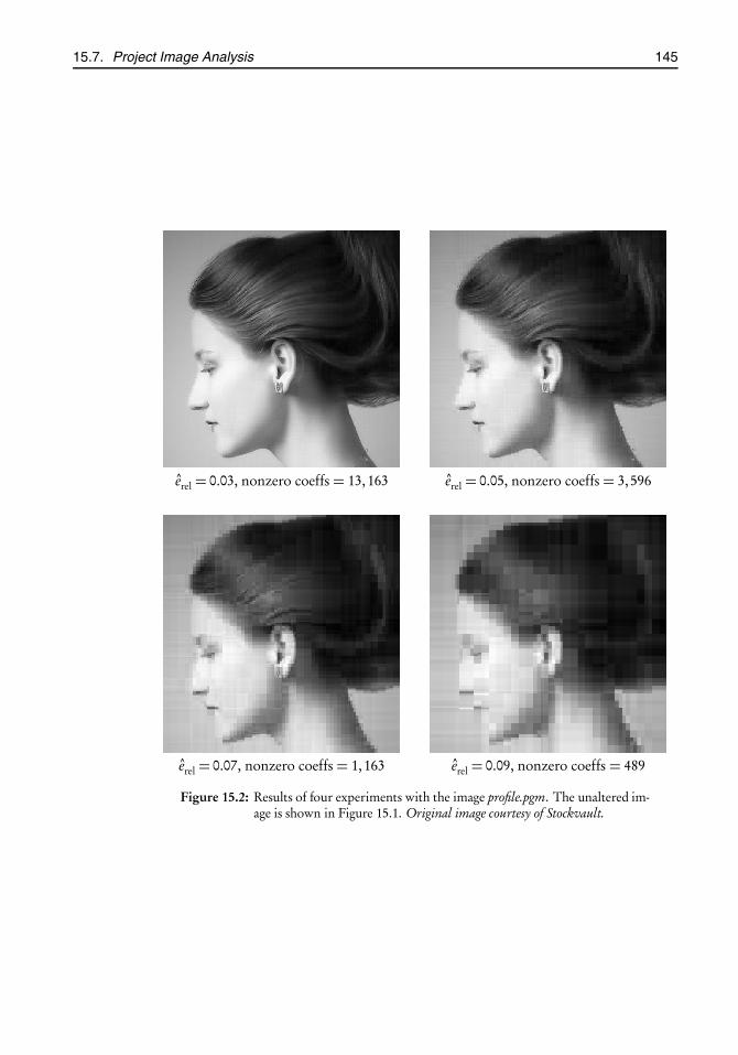
root2014/7/8page 145
�
�
�
�
�
�
�
�
15.7. Project Image Analysis 145
erel = 0.03, nonzero coeffs = 13,163 erel = 0.05, nonzero coeffs = 3,596
erel = 0.07, nonzero coeffs = 1,163 erel = 0.09, nonzero coeffs = 489
Figure 15.2: Results of four experiments with the image profile.pgm. The unaltered im-age is shown in Figure 15.1. Original image courtesy of Stockvault.

root2014/7/8page 147
�
�
�
�
�
�
�
�
Chapter 16
Linked lists
Prerequisite: Chapter 7
16.1 Linked listsA linked list is a data structure consisting of objects called nodes, where each node con-sists of a pointer to user-supplied data and a pointer to the next node, as shown in thisschematic diagram:
list
data data
· · ·
data
NULL
The last node has no successor; therefore its next-node pointer is NULL. Access to thelinked list is provided through a pointer to the first node—it’s markedlist in the diagramabove, but you may name it anything you wish. Beginning with list, we may hop froma node to the next following the next-node pointers and thus traverse the entire list. Whenwe arrive at NULL, we know we’re at the end. The C idiom for traversing a linked list is
for (p = list; p �= NULL; p = p→next {... do whatever with p ...
}
where p has the type of a “pointer to node”.Linked lists are particularly useful when dealing with collections of variable size. For
instance, in the evolution model of Chapter 17 we keep track of the “animals” in thesimulated world by chaining them into a linked list. When an animal dies, we remove thecorresponding node from the list. When an animal is born, we insert a node in the list.Thus, the linked list shrinks and expands as the animal population changes.
C has no standardized linked lists facility. Some other languages do. The containerslibrary in C++, for instance, provides extensive support for linked lists. The Lisp pro-gramming language and its derivatives have linked lists as their primary data types. (Thename “Lisp” is derived from “List processing”.) This chapter’s algorithms for manipulat-ing linked lists are influenced by Lisp and Lisp idioms.
147
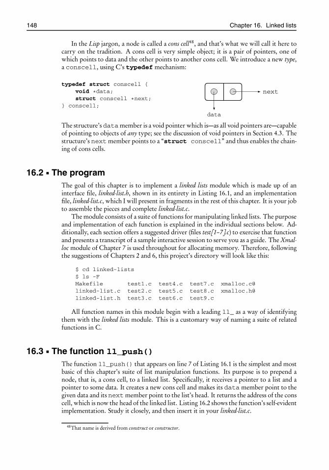
root2014/7/8page 148
�
�
�
�
�
�
�
�
148 Chapter 16. Linked lists
In the Lisp jargon, a node is called a cons cell48, and that’s what we will call it here tocarry on the tradition. A cons cell is very simple object; it is a pair of pointers, one ofwhich points to data and the other points to another cons cell. We introduce a new type,a conscell, using C’s typedef mechanism:
typedef struct conscell {void *data;struct conscell *next;
} conscell;
data
next
The structure’s datamember is a void pointer which is—as all void pointers are—capableof pointing to objects of any type; see the discussion of void pointers in Section 4.3. Thestructure’s next member points to a “struct conscell” and thus enables the chain-ing of cons cells.
16.2 The programThe goal of this chapter is to implement a linked lists module which is made up of aninterface file, linked-list.h, shown in its entirety in Listing 16.1, and an implementationfile, linked-list.c, which I will present in fragments in the rest of this chapter. It is your jobto assemble the pieces and complete linked-list.c.
The module consists of a suite of functions for manipulating linked lists. The purposeand implementation of each function is explained in the individual sections below. Ad-ditionally, each section offers a suggested driver (files test[1–7].c) to exercise that functionand presents a transcript of a sample interactive session to serve you as a guide. The Xmal-loc module of Chapter 7 is used throughout for allocating memory. Therefore, followingthe suggestions of Chapters 2 and 6, this project’s directory will look like this:
$ cd linked-lists$ ls -FMakefile test1.c test4.c test7.c [email protected] test2.c test5.c test8.c [email protected] test3.c test6.c test9.c
All function names in this module begin with a leading ll_ as a way of identifyingthem with the linked lists module. This is a customary way of naming a suite of relatedfunctions in C.
16.3 The function ll_push()
The function ll_push() that appears on line 7 of Listing 16.1 is the simplest and mostbasic of this chapter’s suite of list manipulation functions. Its purpose is to prepend anode, that is, a cons cell, to a linked list. Specifically, it receives a pointer to a list and apointer to some data. It creates a new cons cell and makes its data member point to thegiven data and its next member point to the list’s head. It returns the address of the conscell, which is now the head of the linked list. Listing 16.2 shows the function’s self-evidentimplementation. Study it closely, and then insert it in your linked-list.c.
48That name is derived from construct or constructor.

root2014/7/8page 149
�
�
�
�
�
�
�
�
16.3. The function ll_push() 149
Listing 16.1: The header file linked-list.h provides the interface of the linked lists module.
1 #ifndef H_LINKED_LISTS_H2 #define H_LINKED_LISTS_H3 typedef struct conscell {4 void *data;5 struct conscell *next;6 } conscell;7 conscell *ll_push(conscell *list, void *data);8 conscell *ll_pop(conscell *list);9 void ll_free(conscell *list);
10 conscell *ll_reverse(conscell *list);11 conscell *ll_sort(conscell *list,12 int (*cmp)(const void *a, const void *b, void *params),13 void *params);14 conscell *ll_filter(conscell *list,15 int (*filter)(const void *a),16 conscell **removed);17 int ll_length(conscell *list);18 #endif /∗ H_LINKED_LISTS_H */
Listing 16.2: The function ll_push() in linked-list.c prepends a node to a linked list.
1 conscell *ll_push(conscell *list, void *data)2 {3 conscell *new = xmalloc(sizeof *new);4 new→data = data;5 new→next = list;6 return new;7 }
16.3.1 A demo of ll_push(): test1.c
The file test1.c in Listing 16.3 provides a driver demonstrating a typical use ofll_push().It begins with an empty linked list, then pushes four items into it, and then scans the listand prints the data values stored in it. Let’s go through the code line by line:
Line 5. The list variable declared here points to the first element of our linked list. Itis initialized to NULL, indicating that the list is empty, i.e., it has no nodes.
Line 6. A few arbitrary numbers are introduced here to serve as data in our demonstra-tion.
Line 7. We pass the address of the first number, &a, toll_push(), which creates a conscell and prepends it to the list and returns the address of the updated list. We updatethe value of list by assigning the new address to it. The next three lines repeatthe process with &b, &c, and &d.
Line 12. We traverse the list and print the data stored in it. Since the data pointers arevoid pointers, they cannot be dereferenced as they are; that’s the reason for castingp→data to (int *) before dereferencing.

root2014/7/8page 150
�
�
�
�
�
�
�
�
150 Chapter 16. Linked lists
Listing 16.3: File test1.c provides a demo of ll_push(). It begins with an empty linked list andthen pushes four items into it.
1 #include <stdio.h>2 #include "linked-list.h"3 int main(void)4 {5 conscell *list = NULL; // an empty list6 int a = 101, b = -45, c = 1000, d = 12;7 list = ll_push(list, &a);8 list = ll_push(list, &b);9 list = ll_push(list, &c);
10 list = ll_push(list, &d);11 printf("the original linked list:\n");12 for (conscell *p = list; p �= NULL; p = p→next)13 printf("%d ", *(int *)p→data);14 putchar(’\n’);15 return 0;16 }
We compile the program into an executable called test1 and run it. We get
$ ./test1the original linked list:12 1000 -45 101
Note the reversed order relative to the original a, b, c, and d. Can you explain why thathappens?
Remark 16.1. Don’t take the program in test1.c as a finished product. A well-behavedprogram will free all allocated memory before it exits. This one doesn’t. You may wantto return here and fix test1.c after you read about ll_free() in Section 16.5.
16.4 The function ll_pop()
The function ll_pop() that appears on line 8 of Listing 16.1 is almost an inverse ofll_push()—it removes a linked list’s head node. Specifically, it frees the memory allo-cated previously for that node’s cons cell and returns the address of the list’s new head.We design ll_pop() so that it is safe to call it with an empty list; since there are no nodesto remove, it will do nothing. Generally, the function is used as
list = ll_pop(list);
After popping a node, the associated data becomes inaccessible. Grab and save the data ifyou are going to need it. If you have explicitly allocated memory for the data, it is yourresponsibility to free that memory before you pop the node. The function ll_pop()itself has no knowledge of the nature of data that the cons cell points to.
Write an implementation of ll_pop()—it’s not hard—and add it to your linked-list.c.
16.4.1 A demo of ll_pop(): test2.c
Copy test1.c to test2.c, and add code to pop two nodes then print the result. Then popthree more nodes and print the result. Here’s what mine says:

root2014/7/8page 151
�
�
�
�
�
�
�
�
16.5. The function ll_free() 151
$ ./test2the original linked list:12 1000 -45 101the list after popping two nodes:-45 101the list after popping three more nodes:
The last step prints nothing because the list is empty. Note that applying ll_pop()five times to a linked list of four nodes is permissible according to our specifications ofll_pop().
16.5 The function ll_free()
The function ll_free() that appears on line 9 of Listing 16.1 frees the memory allo-cated for all the cons cells of a linked list. Normally you will apply ll_free() to a linkedlist when you are done with it.
Have in mind that ll_free() has no knowledge of the nature of the data that thelist’s nodes point to. If you have explicitly allocated memory for the data, you will haveto traverse the list and free that memory before calling ll_free().
Here is a possible implementation of ll_free():
void ll_free(conscell *list) // version 1: iterative{
while (list �= NULL) {conscell *p = list→next; // remember the next nodefree(list); // free the head nodelist = p; // produce a shorter list
}}
Note the delicate “tap dance” there. If we free a node prematurely, we will lose its next-node pointer and therefore will be cut off from the rest of the list. The trick is to lookone node ahead and save its address before freeing the current node.
The implementation above is an iterative algorithm—it walks through the linked listin a while-loop and performs an operation on each node until it reaches the end. Al-ternatively, ll_free() may be implemented in a recursive algorithm that takes quite adifferent point of view. I will describe the very Lisp-ish algorithm in words first:
1. If the list is empty, then there is nothing to do.2. Otherwise detach and free the head node and apply ll_free() to the rest of the
list.
Here is the C implementation of that algorithm. Note that in contrast to the iterativeversion, this one has no explicit looping constructs at all!
void ll_free(conscell *list) // version 2: recursive{
if (list �= NULL) {conscell *p = list→next; // remember the next nodefree(list); // free the head nodell_free(p); // recurse: free the rest of the list
}}

root2014/7/8page 152
�
�
�
�
�
�
�
�
152 Chapter 16. Linked lists
Choose one or the other implementation of ll_free(), and insert it in your linked-list.c. They have equivalent effects, so the choice does not matter for our purposes, but itwould be an excellent idea if you tried both methods for the sake of experimentation.
16.5.1 A demo of ll_free(): test3.c
Copy test1.c to test3.c. Add code to free the linked list before exiting, and print what itdoes, as in
ll_free(list);printf("linked list memory freed\n");
Here is what mine says:
$ ./test3the original linked list:12 1000 -45 101linked list memory freed
Remark 16.2. The ll_free() function frees the memory allocated for a linked list’scons cells. It does nothing to free the memory allocated, if any, for the correspondingdata. It is the programmer’s responsibility to free all memory associated with the databefore calling ll_free(). To make this chapter’s examples as simple as possible, I havelimited the sample data to numerical values that require no memory allocation and there-fore no freeing. In the more practical instances that we will encounter in the future chap-ters, memory for data is always allocated and must be freed.
Remark 16.3. After ll_free(list) returns, the value of list is meaningless; itpoints to an area of memory that no longer belongs to you, and of course you should noteven consider referring to it. Generally this is not a problem—why would you want torefer to a nonexistent list, anyway?—but some programmers derive comfort from settingthe value of a freed pointer to NULL. If that’s what you want, then you will have to setlist = NULL explicitly after ll_free(list) returns.
Alternatively, you may redesign ll_free() completely so that instead of list, ittakes the list’s address, as in ll_free(&list), for argument. It this way it will knowwhere list is stored, and therefore it will be able to set it to NULL before it returns, thusfreeing the caller from the concern of NULL-ing the pointer explicitly. Hanson [26], forinstance, takes this approach.
16.6 The function ll_reverse()
You have observed that when we assemble a linked list one node at a time, the list comesout in the reverse order of the insertions. This is not of concern in many cases, but in afew cases where it is, we should like to be able to reverse the order of the nodes of a givenlist. The function ll_reverse() that appears on line 10 of Listing 16.1 on page 149does exactly that. It receives a list and returns the address of the reversed list:
list = ll_reverse(list);
An algorithm for ll_reverse() may not be immediately obvious—I know, it wasn’tobvious to me the first time I thought about it—but once you see it, it turns out to beabsolutely trivial. I urge you, therefore, to stop reading now and spend a few minutesthinking about how you would go about reversing a linked list. After you figure it out (orif you give up) come back and read on.

root2014/7/8page 153
�
�
�
�
�
�
�
�
16.7. The function ll_sort() 153
The idea is this: think of two lists, list1 which is the original one, and list2 which isinitially empty. Remove the first node from list1, and prepend it to list2. Repeat untillist1 is exhausted. Then list2 is the desired reversed list. Return list2 to the caller. Done.
Write an implementation of the ll_reverse(), and add it to your collection inlinked-list.c.
16.6.1 A demo of ll_reverse(): test4.c
To test your work, copy test3.c to test4.c. Reverse the original list, and print it out. Hereis what mine says:
$ ./test4the original linked list:12 1000 -45 101the reversed linked list:101 -45 1000 12linked list memory freed
16.7 The function ll_sort()
The purpose of the function ll_sort() that appears on line 11 of Listing 16.1 onpage 149 is to reorder a list’s nodes according to a prescribed comparison criterion. Thedeclaration ofll_sort() in that listing is somewhat long; therefore I have broken it intothree lines. This should not obscure the fact that ll_sort() takes three arguments:
1. The first argument, list, points to the linked list to be sorted.2. The second argument, cmp(), is a user-supplied comparison function which con-
forms to the prototype
int cmp(const void *a, const void *b, void *params);
and which is the subject of subsection 16.7.1.3. The third argument, params, is a pointer to a set of parameters which the compar-
ison function may or may not need. The function ll_sort() passes that pointerto the comparison function whenever it calls it.
The function ll_sort() returns a pointer to the head of the reordered list; therefore atypical call looks like this:
list = ll_sort(list, cmp, params);
If the comparison function has no use for parameters, then passing NULL for paramswill do
list = ll_sort(list, cmp, NULL);
In the next subsection I will elaborate on the nature of the comparison function. Inthe subsection after that I will describe the sorting algorithm.
16.7.1 The comparison function
I will explain the specifics of ll_sort()’s comparison function through the followingtwo examples.
Example 1: Suppose the data associated with each node is an integer. We wish to sort thelist in the increasing (or decreasing) order of those numbers.

root2014/7/8page 154
�
�
�
�
�
�
�
�
154 Chapter 16. Linked lists
Example 2: Suppose the data associated with each node is a coordinate pair (x, y). Wewish to sort the list according to increasing distances away from a given point p =(x0, y0).
In each case the comparison function takes a pair of data items and decides which oneshould come first in the list. Customarily, a compassion function cmp(a,b) returnsan integer less than, greater than, or equal to zero if the first argument is considered tobe “less than”, “greater than”, or “equal” the second, respectively, for sorting purposes.A reasonable comparison function for Example 1 above would be
int cmp1(int a, int b) // tentative{
if (a < b)return -1;
else if (a > b)return 1;
elsereturn 0;
}
For Example 2 it would make sense to introduce a structure to hold a coordinate pair
struct point { double x; double y; };
and then pass the addresses of such structures to the comparison function, as in
int cmp2(struct point *a, struct point *b, struct point *p) // tentative{
double dx, dy, d1, d2;dx = a→x - p→x; // the x distance of a from pdy = a→y - p→y; // the y distance of a from pd1 = dx*dx + dy*dy; // square of distance of a from pdx = b→x - p→x; // the x distance of b from pdy = b→y - p→y; // the y distance of b from pd2 = dx*dx + dy*dy; // square of distance of b from pif (d1 < d2)
return -1;else if (d1 > d2)
return 1;else
return 0;}
The function calculates the distances (actually the squares of the distances) of the pointsa and b from p and returns -1, 0, or +1 depending on the relationship between thosedistances.
Unfortunately neither of the two preceding comparison functions is suitable for ourpurposes since their arguments are so tightly coupled with their data types. We want thesorting function ll_sort() to be generic, that is, applicable to any linked list, regardlessof the associated data types. With that in mind, we postulate a universal comparisonfunction in the form49
int cmp(const void *a, const void *b, void *params);
49The purpose of the const qualifiers here is to reassure the compiler that the data that a and b point to willbe read but not modified. This can help the compiler produce a better optimized code; otherwise they are notessential. Don’t worry about them if they look unfamiliar.

root2014/7/8page 155
�
�
�
�
�
�
�
�
16.7. The function ll_sort() 155
Since a void pointer is compatible with pointers to all data types, this form of the com-parison function is ideal; pointers to data of any type may be passed to it. The function’sfirst two arguments point to the items that are to be compared. The third argument pointsto parameters that may or may not be useful for the purpose of that comparison. Modi-fying the previous comparison function cmp1() into the new form, we arrive at
int cmp1(const void *aa, const void *bb, void *pp) // correct form{
int a = *(int *)aa;int b = *(int *)bb;if (a < b)
return -1;else if (a > b)
return 1;else
return 0;}
The function casts the void pointer aa to a pointer-to-int and then dereferences it toobtain its value, a. It does the same with bb. Then it proceeds just as in the previousversion of cmp1(). The parameter pp is not used. Similarly, the modified version ofcmp2() takes the form
int cmp2(const void *aa, const void *bb, void *pp) // correct form{
struct point *a = (struct point *)aa;struct point *b = (struct point *)bb;struct point *p = (struct point *)pp;double dx, dy, d1, d2;
dx = a→x - p→x;dy = a→y - p→y;d1 = dx*dx + dy*dy; // square of distance of a from pdx = b→x - p→x;dy = b→y - p→y;d2 = dx*dx + dy*dy; // square of distance of b from pif (d1 < d2)
return -1;else if (d1 > d2)
return 1;else
return 0;}
Nowcmp1() andcmp2() have identical signatures/prototypes, and that’s what matters.Their innards are quite different.
16.7.2 Quicksort
Sorting is a huge subject and there are books written on it. See, e.g., Knuth’s The Art ofComputer Programming [34]. I will describe what is known as the quicksort algorithm,which, in its recursive form, is particularly well suited to sorting linked lists. Here is thealgorithm in words:

root2014/7/8page 156
�
�
�
�
�
�
�
�
156 Chapter 16. Linked lists
the original list (unsorted)1.
list12. list2head
sorted list13. sorted list2head
the reassembled (sorted) list4.
Figure 16.1: This diagram shows the four steps of the quicksort algorithm. Line 1 rep-resent the original (unsorted) list. In line 2 we have isolated the list’s headand split the rest into list1 and list2, where all items in list1 are “less than”the head (according to the comparison criterion) and list2 consists of what’sleft. In line 3 we have sorted list1 and list2, and in line 4 we have pasted thethree pieces to form a completely sorted list.
1. If the list is empty, there is nothing to do. The result is the empty list.2. Otherwise, detach the list’s first node (the head) and set it aside. Split the rest into
two lists, list1 and list2, where list1 consists of all the nodes that are “less than” thefirst node (according to the comparison function) and list2 consists of the others.
3. Sort list1 and list2.4. Reassemble the list as list1 →head→list2. This is the desired sorted list.
The procedure is highly recursive since the sorting of the sublists list1 and list2 in step 3invokes the sorting procedure all over again. Figure 16.1 shows the procedure in a dia-grammatic way. Listing 16.4 gives a quite literal implementation of that algorithm in C.Study Listing 16.4 carefully, and be sure that you understand every bit of it; then add itto your linked-list.c.
Remark 16.4. Although the ll_sort() function is unabashedly recursive in its out-line, the while-loop embedded in the middle of Listing 16.4 is iterative. Is it possi-ble to replace it with recursion as well? Certainly! The purpose of that while-loopis to split a given list into list1 and list2 according to a given criterion. The functionll_filter(), which is the subject of the next section, does exactly that and is strictlyrecursive. Therefore one may, in principle, replace the while-loop in ll_sort() witha call to ll_filter() and obtain a purely recursive ll_sort(). Unfortunately thecoding details of passing arguments from ll_sort() to ll_filter() become some-what cumbersome and obscure the conceptual simplicity of the underlying idea.50 Youmay want to try it for yourself to see that.
16.7.3 A demo of ll_sort(): test5.c
To test/demoll_sort(), copy test3.c to test5.c. Add two comparison function, cmp1()and cmp2(), one for sorting the linked list in the ascending order of its numerical dataand the other in the descending order. Compile and run the program. Here is what minesays:
50This is not a shortcoming of the idea. Rather, it is an indication that we have reached the limits of what onemay express comfortably in C. A functional programming language, such as Lisp, on the other hand, can expressthe idea elegantly and succinctly.
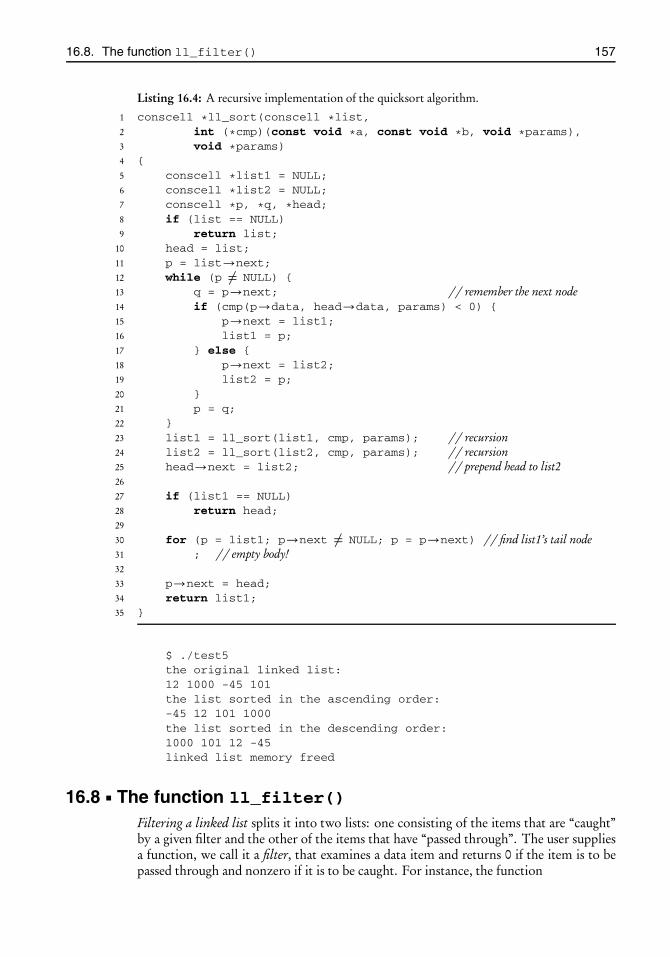
root2014/7/8page 157
�
�
�
�
�
�
�
�
16.8. The function ll_filter() 157
Listing 16.4: A recursive implementation of the quicksort algorithm.
1 conscell *ll_sort(conscell *list,2 int (*cmp)(const void *a, const void *b, void *params),3 void *params)4 {5 conscell *list1 = NULL;6 conscell *list2 = NULL;7 conscell *p, *q, *head;8 if (list == NULL)9 return list;
10 head = list;11 p = list→next;12 while (p �= NULL) {13 q = p→next; // remember the next node14 if (cmp(p→data, head→data, params) < 0) {15 p→next = list1;16 list1 = p;17 } else {18 p→next = list2;19 list2 = p;20 }21 p = q;22 }23 list1 = ll_sort(list1, cmp, params); // recursion24 list2 = ll_sort(list2, cmp, params); // recursion25 head→next = list2; // prepend head to list226
27 if (list1 == NULL)28 return head;29
30 for (p = list1; p→next �= NULL; p = p→next) // find list1’s tail node31 ; // empty body!32
33 p→next = head;34 return list1;35 }
$ ./test5the original linked list:12 1000 -45 101the list sorted in the ascending order:-45 12 101 1000the list sorted in the descending order:1000 101 12 -45linked list memory freed
16.8 The function ll_filter()
Filtering a linked list splits it into two lists: one consisting of the items that are “caught”by a given filter and the other of the items that have “passed through”. The user suppliesa function, we call it a filter, that examines a data item and returns 0 if the item is to bepassed through and nonzero if it is to be caught. For instance, the function

root2014/7/8page 158
�
�
�
�
�
�
�
�
158 Chapter 16. Linked lists
int catch_the_odds(int a) // tentative form{
return a%2;}
is a filter that catches odd integers and lets the evens pass through. For the reasons ex-plained in the previous section, this function will have to be modified into the genericform
int catch_the_odds(void *aa) // correct form{
int a = *(int *)aa;return a%2;
}
in order to mesh with the ll_filter() function which we intend to develop in thissection and which appears on line 14 of Listing 16.1 on page 149. The declaration ofll_filter() in that listing is long; therefore I have broken it into three lines. Thefunction takes three arguments:
1. The first argument, list, points to the linked list that is to be filtered.2. The second argument, filter(), is a user-supplied filter function as described
above.3. The third argument, removed, is the address of a pointer to the linked list of the
items caught by the filter.
The function returns the linked list of the items that pass through the filter. A typical useof the filter() takes the form
conscell *list, *removed = NULL;... create the list, then ...list = ll_filter(list, filter, &removed);
After the last line, removed points to the linked list of the caught items, and listpoints to the linked list of the items that have passed through.
As to the implementation of ll_filter(), both iterative of recursive strategies arepossible. In the iterative strategy we keep track of the address of the previous node aswe traverse the list. If the current node is to be removed, we make the current node’sprevious node point to the current node’s next node. I will leave it to you to implementthis if you wish. It’s an instructive exercise; try it, it’s not very hard.
The recursive strategy, again very Lisp-ish, is short and sweet. Here it is in words:
1. If the list is empty, there is nothing to do; return the empty list.2. Otherwise, if the filter catches the list’s head, (a) detach the head from the list, (b) at-
tach it to the removed list, and (c) filter and return the rest of the list.3. Otherwise (a) detach the head from the list, (b) filter the rest of the list, (c) reattach
the head, and (d) return the list.
This maps essentially word for word to C. Study the following code, and then insert itinto your linked-list.c:
conscell *ll_filter(conscell *list,int (*filter)(const void *a), conscell **removed)
{if (list == NULL)

root2014/7/8page 159
�
�
�
�
�
�
�
�
16.10. Project Linked Lists 159
return list;else if (filter(list→data)) {
conscell *p = list→next; // remember the next nodelist→next = *removed;
*removed = list;return ll_filter(p, filter, removed);
} else {list→next = ll_filter(list→next, filter, removed);return list;
}}
16.8.1 A demo of ll_filter(): test6.c
To test/demo ll_filter(), copy test3.c to test6.c, define a filter that catches the oddintegers, apply the filter to the existing linked list, and print the caught and passed throughlists. Here is what mine says:
$ ./test6the original list:12 1000 -45 101the list after removing the odds:12 1000these items were removed:101 -45memory of passed-through list freedmemory of caught list freed
16.9 The function ll_length()
The function ll_length(), whose prototype is given on line 17 of Listing 16.1 onpage 149, returns the length, that is, the number of nodes, of a linked list. As with theother ll_*() functions, this may also be implemented in an iterative or recursive fash-ion. Write one or the other version (or both!), and insert it in your linked-list.c.
To test/demo your work, copy test3.c to test7.c and add code to write and print thenumber of nodes. Here is what mine says:
$ ./test7the original linked list:12 1000 -45 101the list has 4 nodeslinked list memory freed
16.10 Project Linked Lists
Part 16.1. Complete and test your linked-list.[ch] and the driver files test[1–7].c as in-structed in the preceding sections.
Part 16.2. [optional] Our ll_sort() handles comparison functions which may de-pend on a parameter (which we named params). Modify the function ll_filter()to handle filter functions that depend on a parameter in a similar way.

root2014/7/8page 160
�
�
�
�
�
�
�
�
160 Chapter 16. Linked lists
Part 16.3. [optional] Extend the linked lists module by adding a function ll_append()with the prototype
conscell *ll_append(cons struct *list1, cons struct list2);
which concatenates list1 and list2; that is, it makes list1’s last node point tolist2’s first node. It returns the address of the new list. The return value is redun-dant since it is no different from the address of list1. Nonetheless, it is a nice touch todo so since that conforms to the style of the other ll_*() functions.
Write a driver, test8.c, to test/demonstrate the function.
Part 16.4. [optional] Extend the linked lists module by adding a function ll_map()with the prototype
conscell *ll_map(conscell *list, void (*map)(void *data));
which applies a given function, map(), to the data at every node of a linked list. Forinstance, if we let
void square_me(void *data){
int *n = data;
*n = (*n) * (*n);}
then calling list = ll_map(list, square_me) with test1.c’s linked list shouldproduce
$ ./test9the original list:12 1000 -45 101the squared list:144 1000000 2025 10201linked list memory freed
Write a driver, test9.c, to demonstrate this.
root2014/7/8page 161
�
�
�
�
�
�
�
�
Chapter 17
The evolution of species
Prerequisites: Chapters 7, 8, 9, 10, 16
17.1 IntroductionIn the late 1980s Michael Palmiter devised a very simple model of evolution by naturalselection which exhibited a strikingly realistic behavior.51 A. K. Dewdney popularized itin a Scientific American article [17]. I learned about these from Conrad Barski’s book [7],where he develops a variant of the simulation in Lisp. In this chapter we will write aC version and introduce variations of our own. The models appear to be quite robustand insensitive to the details of the evolutionary mechanisms in the sense that all variantsexhibit similar evolutionary characteristics.
The simulation begins with one or more individuals endowed with random geneticstructures whose descendants reproduce, evolve, and gradually adapt to their environ-ments in the course of many (millions of) generations. In the long run, genetically distinctpopulations emerge in environmentally distinct regions of the simulated world.
Let me first briefly describe a rough overview of the basic ideas; then I will supply thedetails.
In the simulation, time flows in discrete “time ticks”. The “world” consists of a two-dimensional rectangular grid of cells. “Animals” move about in the world, hopping froma cell to an adjacent cell at each time tick, expending a certain amount of energy on eachhop. If an animal’s energy drops to zero, it dies and is removed from the simulation.Food sprouts in random cells. If an animal stumbles upon a cell containing food, it eatsthe food and gains energy. If an animal’s energy increases past a certain threshold (thereproduction threshold), it splits into two animals in a manner of asexual reproduction,and each of the two inherits half of the parent’s energy.
Each animal is endowed with a “chromosome” which is a vector of length 8 of positiveintegers. The chromosome remains unchanged over an animal’s lifetime. The vector’seight entries are the “genes”. If one or more of an animal’s genes are distinctly greaterthan the rest, we say that those are its “dominant genes”. The chromosome is the onlycharacteristic that distinguishes one animal species from another in this model.
At every time tick one of the animal’s eight genes, selected at random, becomes “acti-vated”. A gene of a larger value has a greater probability of being selected. The activation
51As of this writing (September 2013) Palmiter’s simulated evolution program is available for purchase at<http://lifesciassoc.home.pipeline.com/instruct/evolution/>.
161

root2014/7/8page 162
�
�
�
�
�
�
�
�
162 Chapter 17. The evolution of species
of gene number k, k = 0, . . . , 7, makes the animal rotate in its place by an angle of 45× kdegrees relative to its current orientation. After the rotation, the animal takes one stepforward into the adjacent cell. Thus, an animal with a dominant gene 0 will tend to moveforward along a straight line, while an animal with a dominant gene 2 will tend to goaround in tight circles. An animal’s genetic structure, therefore, affects the mode of itsmovements, which in turn affects its chances of finding food and survival.
An animal inherits its parent’s genetic structure modulo small mutations. If the mu-tations are favorable to survival, then that animal and its descendants thrive. If the muta-tions are unfavorable, the descendants dwindle and die out. In the long run, this leads toa population which is increasingly more adept at survival.
Speciation, that is, the emergence of distinct species, occurs in response to environ-mental pressures. To demonstrate this, we set aside a small area of the world as a fertileregion where food grows more plentifully than elsewhere, which is the desert, and wherefood is sparse.
Simulations show that in the long run two distinct classes of species emerge. Onespecies consists of “desert dwellers” who are compelled by their dominant genes to travelover long distances, whereby increasing their chances of finding the sparsely scatteredfood in the desert. The others live in the fertile region and have dominant genes that limittheir movements to small jitters, thereby keeping them within the fertile region wherefood is plentiful. As Dewdney puts it, “What normally is a disastrous genetic defect isactually an advantage in an overpopulated Garden of Eden.”
Following Dewdney and Palmiter, I will refer to the fertile region as the “Garden ofEden” or simply the “Eden”.
17.2 A more detailed descriptionThe previous section’s brief sketch of the simulation’s setup should give you a reasonablycomplete picture of the scenario which we intend to pursue. In the current section I willdwell on the setup’s details. Thus, without further ado, let us proceed to the descriptionof the simulation’s components.
The world: The “world” is a rectangle whose opposite edges are identified; that is, if ananimal leaves the bottom edge, it emerges from the corresponding spot on the topedge. The left and right edges are identified in a similar way.52 This obviates theneed for boundary conditions and thereby simplifies the model.
The world rectangle is discretized into an h×w grid of cells. The time is discretizedinto discrete time-steps. We refer to the cell in the world’s ith row and j th columnas the cell (i , j ) in analogy to the customary addressing of the rows and columnsof a matrix, but in contrast with matrices, our indices begin at zero. Figure 17.1(a)shows a (much too small) 6×8 world. A 100×100 world is much more interestingfor simulations. Each cell has eight neighboring cells, numbered 0, . . . , 7, as shownin the diagram of Figure 17.1(b). For a cell near an edge of the rectangle, neigh-boring cells wrap around to the opposite edge according to the world’s toroidalstructure.
In the future we will have occasions to refer to the world’s “center” cell, which is acell that is closest to the world rectangle’s center. If h and w are odd, then the (i , j )index of the center cell is exactly
�(h − 1)/2, (w − 1)/2
. (You will have to draw a
little picture to see that. Remember that cell indices begin with zero.) For general
52A topologist would say that this world is a torus or has a toroidal topology.

root2014/7/8page 163
�
�
�
�
�
�
�
�
17.2. A more detailed description 163
food in cell (1,6)
animal in cell (0,0)
animal in cell (3,4)
j
i
(a) A 6× 8 world with a 2× 2 Eden
01
2
34
5
6
7
(b) A cell and its neighbors
Figure 17.1: The diagram on the left shows a (much too small) 6× 8 world. There is a2× 2 Eden at the center. The i and j arrows at the top left are remindersthat cells are indexed as in a matrix—from left to right in columns, fromtop to bottom in rows. The diagram on the right shows a generic cell andits eight neighboring cells, which are numbered 0 through 7.
h and w, we define the center cell by rounding the fractions to integers according to
world’s center cell=!"
h − 1
2
#,"
w − 1
2
#$. (17.1)
The notation �x� indicates the greatest integer less than or equal to x. For non-negative integers p and q , the quotient p/q in C is evaluated to
%p/q
&by default;
therefore no special effort is required to evaluate the expression in (17.1).
The Eden: The Eden is a rectangular subset of the world which has a richer than normalfood supply. The spatial inhomogeneity due to the presence of the Eden leads tospeciation, that is, the emergence of genetically distinct species. Figure 17.1(a) showsa 2×2 Eden in a 6×8 world. Setting one or both of Eden’s dimensions to zero eliminatesthe Eden altogether.
The world’s toroidal structure implies that the Eden’s location within the world isimmaterial; all placements of the Eden are equivalent for the purposes of the simu-lation. The Eden’s location, however, does affect the ease of some of the computa-tions. Specifically, to interpret the simulation’s results, it is essential, as we shall seelater, to sort the animals according to their distances away from the Eden. Calcu-lating such distances is easy if the Eden is located at or near the world’s center cellsince the concept of the distance then coincides with the usual notion of distance.If, however, the Eden is placed off center, then the distance calculations becomeslightly more involved due to the wrapping of the rectangle’s edges. For this rea-son, I will assume from now on that the Eden is “centered” on the world rectangleas best as possible. Specifically, let the Eden be an h ′ × w ′ rectangle of cells. Weposition the Eden so that the cell at its northwest corner coincides with the world’s

root2014/7/8page 164
�
�
�
�
�
�
�
�
164 Chapter 17. The evolution of species
cell (i , j ), where
(i , j ) =!"
h − 1
2
#,"
w − 1
2
#$−!"
h ′ − 1
2
#,"
w ′ − 1
2
#$. (17.2)
Convince yourself that this centers the Eden in a best possible way relative to theworld. Exact centering is not always possible since that depends on the parity of theworld’s and Eden’s dimensions. Deviations from the exact center are insignificantif the world rectangle is large, as it is in our simulations.
When the Eden is positioned according to (17.2), then its “center” cell agrees—modulo the usual parity issues—with the world’s center cell given in (17.1). Werecord this here for future reference:
the Eden’s center cell=
!"h − 1
2
#,"
w − 1
2
#$. (17.3)
Food: At every time-step a morsel of food is dropped (or sprouts) in a randomly selectedcell.53 If an Eden exists, an additional morsel of food is dropped there. A foodmorsel contains a certain amount54 of nutritional energy. A cell may hold morethan one morsel of food.
Animals: Animals move about from cell to cell. Any number of animals may occupy acell simultaneously. At every time-step every animal moves to a neighboring cellaccording to a mechanism that we shall describe. A move costs the animal 1 unitof energy. If the animal’s energy drops to zero, it dies and is removed from thesimulation. If it arrives at a cell that contains one or more morsels of food, it eatsone morsel and gains energy.
Genes: An animal has a “chromosome” ⟨g0, g1, . . . , g7⟩ consisting of eight integer-valued“genes”, with gk ≥ 1 for all k. The chromosome is an intrinsic characteristic of ananimal; it does not change during the animal’s lifetime.
Movement: An animal may face in any of the eight possible directions numbered0,1, . . . , 7, as shown in Figure 17.1(b). At every time-step one of the animal’s eightgenes is randomly selected and “activated”. The activation of the gene gk promptsthe animal to turn in its place by 45× k degrees counterclockwise, relative to itscurrent orientation. It follows that if the animal is facing the direction d (whered ∈ {0,1 . . . , 7}), then after the activation of gene gk it will be facing the directiond + k mod 8.
After turning, the animal steps forward to the neighboring cell that it faces. Thiscompletes a movement cycle.
The probability of the selection of a gene is proportional to the gene’s value. Thatis, a gene of larger value is more likely to be selected. For example, an animal withthe chromosome structure ⟨1,3,42,2,1,3,4,2⟩ will turn 90 degrees in almost everymove since g2 is the dominant gene.
Reproduction: If an animal’s energy exceeds a certain level,55 it splits in two in a man-ner of an asexual reproduction. The two halves are almost identical clones of the
53We assume uniform probability distribution; that is, one cell is as likely to receive a morsel as another.54This is called PlantEnergy in our program.55This is called ReproductionThreshold in our program.

root2014/7/8page 165
�
�
�
�
�
�
�
�
17.3. The World Definition File 165
original, except for (i) each one inherits half of the original’s energy; and (ii) oneof the two may inherit a slightly mutated chromosome, as described in the nextparagraph.
Mutation: When copying a chromosome, we allow for a possible mutation by adding arandomly selected number from the set {−1,0,1} to a randomly selected gene. (Allrandom numbers here are uniformly distributed.) If the gene value drops below 1,we change it back to 1 because we don’t want genes of 0 or negative values.56
This completes the description of our imaginary world. We initialize it with zerofood and just one animal57 with an arbitrary genetic structure but endowed with a largishinitial energy; otherwise it’s likely that it will die before it finds the first food morsel orhas a chance to reproduce.
What becomes of the descendants of that animal in the long run? The principal tenetof the theory of evolution by natural selection is that mutations that are deleterious tosurvival wipe themselves out since, on the whole, animals with such mutations are out-competed by the others; therefore they don’t live long enough to reproduce. Conversely,mutations that are favorable to survival result in animals that successfully reproduce andbring forth descendants who are equally good, if not better, at survival.
Our simulations indicate that in a world without an Eden, the genetics of the pop-ulation evolve so that the genes g0, g1, and g7 gain dominance. These are the genes re-sponsible for propelling the animal more or less in the forward direction. An animal thatcovers large territories has a better chance of encountering food than a sedentary animalthat hovers in a small area waiting for food morsels to drop in its lap.
With the scenario described above, the animal population remains more or less ho-mogeneous because probabilistically each animal is like the other. Simulations show thatthe population evolves en masse toward a more fit species.
The situation is drastically different in the presence of the Eden. Simulations showthat in the long run the animals diverge into two very distinct species:
The desert-dwellers have dominant g0, g1, and g7 genes and consequently mostly moveforward and cover large territories.
The Eden dwellers have dominant g3, g4, and g5 genes and consequently hover in theEden area to partake of its rich food supply.
It is a testimony to the robustness of the natural selection mechanism that a primitivemodel such as the one under consideration here exhibits the characteristic traits of evolu-tion and speciation observed in the much more complex real world.
17.3 The World Definition FileOur program reads the simulation’s parameters from a user-supplied World DefinitionFile (WDF ), a sample of which is shown in Listing 17.1. The WDF is read with the helpof the fetch_line() function developed in Chapter 9 which strips away blank lines,comments, and leading and trailing whitespace from its input. The general form of astripped-down WDF is
56Genes of value zero are not objectionable; they just will have zero probability of getting activated. It maybe worthwhile to experiment with this alternative. I haven’t.
57The program allows initialization with any number of animals, but starting with just one is more striking.

root2014/7/8page 166
�
�
�
�
�
�
�
�
166 Chapter 17. The evolution of species
Listing 17.1: The WDF world-no-eden.wdf defines a world with only one animal and no Eden.The animal is provided with a good amount of initial energy to give it a chance tofind food, and perhaps reach the reproduction threshold, before dying of starvation.
1 # A World Definition File for the evolution simulator2 World 100 100 # height x width3 Eden 0 0 # No Eden!4 Plant Energy 805 Reproduction Threshold 3006
7 # Animals:8 ( 0 0) 0 200 | 5 5 5 5 5 5 5 5 |
1 World h w2 Eden h w3 Plant Energy e4 Reproduction Threshold t5 (n n) n n | n n n n n n n n |6 ...
Line 1 gives the world’s height and width, that is, the number of vertical and horizon-tal cells that make up the world rectangle, and line 2 gives the Eden’s height and width.Lines 3 and 4 give the values of the plant and reproduction threshold energies. Line 5,which specifies the initial state of an animal, may be repeated any number of times (hencethe “...” on line 6) to initialize the world with the desired number and kinds of animals.The n’s in that line stand for integers, not necessarily all the same. Its meaning is betterexplained through the explicit notation
( i j ) d e | g0 g1 g2 g3 g4 g5 g6 g7 |,where (i j ) is the animal’s location (cell index) subject to 0≤ i < h, 0≤ j < w, where hand w are the world’s height and width; d ∈ {0,1, . . . , 7} is the direction that it faces; e isits energy; and g0 through g7 are its gene values, where every gk ≥ 1.
Note that the WDF does not prescribe the Eden’s location relative to the world rect-angle. We are going to use the formula (17.2) for the Eden’s placement.
17.4 The program’s user interfaceOur program reads the simulation’s parameters from the stdin, runs the simulation,and writes the results to the stdout. If specifically requested, it also produces a numberof graphical snapshots of the world which may be viewed individually, or in sequence asan animation as detailed in Sections 17.12 and 17.13.
Let us say that the program’s executable file is named evolution. We invoke it througha command-line of the form
$ ./evolution options <world-no-eden.wdf >outfile.wdf
where world-no-eden.wdf is the WDF shown in Listing 17.1. The output, which is di-rected to a file named outfile.wdf, contains the state of the world after a prescribed numberof time-steps. The format of the output conforms to the specifications of WDF ; therefore

root2014/7/8page 167
�
�
�
�
�
�
�
�
17.5. The program’s components 167
it can be used to reinitialize the simulation if you wish.58 Of course you may name theinput and output files as you wish; the program itself is unaware of those file names. It’syour Unix shell that directs the data flow through the redirection symbols “<” and “>”;see Chapter 3 for an overview of the Unix shell.
The number of time-steps, or updates as we call it in the program, is specified in theoptions part of the command-line. If options is set to 1000000, as in
$ ./evolution 1000000 <world-no-eden.wdf >outfile.wdf
the simulation will perform 1,000,000 updates. The largest possible number you may en-ter here is ULONG_MAX, which is defined in the standard header file limits.h and whichis the largest unsigned long int that your C compiler can handle. On a typicalcomputer nowadays it is likely to be one of 232 − 1 = 4,294,967,295 ≈ 4.3 × 10⁹ or264− 1 ≈ 1.8× 10¹⁹. Beware that if you enter a number larger than ULONG_MAX on thecommand-line, it will be truncated to ULONG_MAX (silently!). In practice, however, thereis not much reason for that many iterations; 10 million updates are more than enough fordemonstrating evolutionary trends and speciation.
If you invoke the program as
$ ./evolution 1000000 20 <world-no-eden.wdf >outfile.wdf
it will perform the 1,000,000 updates as before; then it will take 20 snapshots of the worldinterleaved with 19 updates. The snapshots will be written as Encapsulated PostScript(EPS) files named fig0000.eps, . . . , fig0019.eps. Only then it will write the outfile.wdf andexit.
Why only 19 updates? The sequence of operations consists ofS U S U ... S U S,where S stands for a snapshot and U stands for an update. As you see, there is one lessupdate than there are snapshots. It follows that the command
$ ./evolution 0 1 <world-no-eden.wdf >outfile.wdf
will capture a snapshot of the world’s initial state which can be useful in itself.If you enter unrecognizable options or no options at all, the program prints a brief
usage note and exits:
$ ./evolutionUsage: ./evolution n [f] <infile >outfile
n ≥ 0 : (required) number of updatesf ≥ 0 : (optional) number of snapshots after n updatesReads World Definition from infile, performsn updates, and writes result to outfile
This message is produced through the show_usage() function, which is the subject ofsubsection 17.11.2.
17.5 The program’s componentsThe program relies on Chapter 7’s xmalloc module for allocating memory, Chapter 8’sarray.h for building vectors and matrices, Chapter 16’s linked lists module for managinglinked lists, and Chapter 9’s fetch-line module for reading lines from a WDF . Therefore,
58Actually the output does not record the complete state of the world since our WDF format carries no infor-mation about which cells contain food. Consequently, the information about the food distribution is lost if youstop and restart the program. Part 17.4 of this chapter’s Projects section suggests an extension to the programwhereby the locations of the food morsels are recorded in a WDF .

root2014/7/8page 168
�
�
�
�
�
�
�
�
168 Chapter 17. The evolution of species
Listing 17.2: The file evolution.h.
1 #ifndef H_EVOLUTION_H2 #define H_EVOLUTION_H3 #include "linked-list.h"4 struct animal {5 int i; // row number of animal’s position6 int j; // column number of animal’s position7 int d; // direction the animal is facing: 0, . . . ,78 int e; // animal’s energy9 int genes[8]; // the animal’s chromosome (array of genes)
10 } animal;11 struct world {12 int world_h; // world’s height13 int world_w; // world’s width14 int eden_h; // Eden’s height15 int eden_w; // Eden’s width16 int plant_energy; // plant energy17 int reproduction_threshold; // reproduction threshold18 int **plants; // world_h × world_w array of plants19 conscell *herd; // the head of the linked list of the animals20 };21 #endif /∗ H_EVOLUTION_H */
following the recommendations of Chapters 2 and 6, the program’s directory will looklike this:
$ cd evolution$ ls -FMakefile fetch-line.h@ read.h write.carray.h@ interlude.c world-and-eden.wdf write.hevolution.c linked-list.c@ world-no-eden.wdf [email protected] linked-list.h@ world-to-eps.c [email protected]@ read.c world-to-eps.h
The file named world-and-eden.wdf is just like world-no-eden.wdf of Listing 17.1 exceptthat it has a 10× 10 Eden. To get started with this project, make an evolution directory,create the files world-no-eden.wdf and world-and-eden.wdf, and establish the symlinks asshown above. In the rest of this chapter I will describe the contents of the remaining files.
17.6 The file evolution.hThe file evolution.h, shown in Listing 17.2, declares two structures, one to hold ani-mal properties and the other to hold the world’s properties. The associated commentsshould adequately explain the purpose of every member except, perhaps, the last two ofstruct world.
The plants member points to a matrix of size world_h × world_w. The (i , j )entry of that matrix is the number of food morsels in the world’s cell (i , j ). The herdmember is the head of the linked list of the animals.
Since struct world refers to conscell, and since conscell is declared in theheader file linked-list.h, we #include that header file on line 3.

root2014/7/8page 169
�
�
�
�
�
�
�
�
17.7. The files read.[ch] 169
Listing 17.3: An outline of the file read.c.
1 #include <stdio.h>2 #include "xmalloc.h"3 #include "fetch-line.h"4 #include "linked-list.h"5 #include "read.h"6 #define BUFLEN 10247 � static int get_world_dimens(struct world *world,8 char *str, int lineno) ...9 � static int get_eden_dimens(struct world *world,
10 char *str, int lineno) ...11 � static int get_plant_energy(struct world *world,12 char *str, int lineno) ...13 � static int get_reproduction_threshold(struct world *world,14 char *str, int lineno) ...15 � static struct animal *get_animal_specs(char *str, int lineno) ...16 � static char *fetch_line_aux(char *buf, int buflen,17 FILE *stream, int *lineno) ...18 � int read_wdf(struct world *world) ...
17.7 The files read.[ch]Listing 17.3 shows an outline of the file read.c that defines a function read_wdf()(line 18) whose purpose is to read a WDF and parse its contents. All the other func-tions in read.c are for read_wdf()’s private use; therefore they are declared staticto make them invisible to the outside world. (See Section 1.6 for an explanation of thestatic specifier.) In the following subsections I will describe the roles of the individualfunctions that appear in Listing 17.3.
The function read_wdf() repeatedly calls the function fetch_line() (from thefetch-line module of Chapter 9) to extract nonempty trimmed lines from a WDF thatarrives from the stdin. According to the conventions of a WDF (see Section 17.3), thefirst four such lines are expected to be the specifications of the world’s and the Eden’sdimensions and the plant and reproduction threshold energies. These may be followedby any number of animal specification lines. Altogether, there are five distinct types oflines that we expect to encounter; therefore we write five distinct function to handle thosetypes. These are the functions
get_world_dimens() get_reproduction_threshold_energy()get_eden_dimens() get_plant_energy()get_animal_specs()
that appear on lines 7 through 15 of Listing 17.3. I will describe the details of these andthe related functions in the following subsections.
17.7.1 The function get_world_dimens() and friends
The function get_world_dimens() that appears on line 7 of Listing 17.3 is respon-sible for parsing the first line of a WDF , which is expected to be a string of the form"World h w", where the integers h and w are the world’s height and width. If thestring is properly formed, get_world_dimens() extracts the numbers h and w, storesthem in the world_h and world_w members of the struct world, and returns 1 to

root2014/7/8page 170
�
�
�
�
�
�
�
�
170 Chapter 17. The evolution of species
Listing 17.4: The function get_world_dimens() in the file read.c.
1 static int get_world_dimens(struct world *world, char *str, int lineno)2 {3 if (sscanf(str, "World %d %d",4 &world→world_h, &world→world_w) == 2)5 return 1;6 else {7 fprintf(stderr, "stdin:line %d: expected to find "8 "World dimensions here\n", lineno);9 return 0;
10 }11 }
indicate success. Otherwise the line is garbled; therefore it prints a diagnostic on thestderr and returns 0 to indicate failure. Listing 17.4 shows my implementation ofget_world_dimens(). The function receives a pointer to struct world whereit will store the world’s height and width; a pointer to the string to parse; and the linenumber of the string as it was read from the stdin. The error diagnostic prints that linenumber to help the user locate the trouble spot.
The standard library function sscanf() returns the number of successfully matchedand assigned items in the call. Therefore, if the input string is properly formed, we expectsscanf() to return 2. That’s what we are checking on line 3 of Listing 17.4.
I will let you write the functions get_eden_dimens(), get_plant_energy(),and get_reproduction_threshold_energy() that appear in Listing 17.3. Theseare close variants of get_world_dimens(). Add your implementations to read.c.
17.7.2 The function get_animal_specs()
The purpose of the function get_animal_specs() that appears on line 15 of List-ing 17.3 is to read the specifications of one animal in a WDF . (Refer to the sample WDFin Listing 17.1 on page 166 regarding animal specifications.) As such, it is very similar tothe previous subsection’s get_world_dimens() function. Nevertheless, I have shownthe entire function in Listing 17.5 because there is a slight twist.
The call to sscanf() works exactly as before, but it is reading 12 integers now. Ifsscanf() returns other than 12, get_animal_specs() prints the usual diagnosticmessage and returns NULL to indicate failure. Otherwise it stores the 12 numbers in astruct animal. This is where the new aspect comes in; the structure has to be created.So it calls xmalloc() to allocate memory for a struct animal and populates it withthe values retrieved by sscanf(). Finally it returns a pointer to the structure to thecalling function. Note that unlike the previous section’s get_*() functions that returnint, this one returns a pointer to a struct animal on success or NULL on failure.
17.7.3 The function fetch_line_aux()
The function fetch_line_aux() that appears on line 16 of Listing 17.3 is a helperfunction which plays no deep role but is quite convenient for our purposes. Recall thatthe function fetch_line() which we developed in Chapter 9 returns NULL whenthe input is exhausted. In the context of reading a WDF , if the end of the input oc-curs after all the required data is in, the situation is normal; we expect that to happen.If, however, the end of the input occurs before all the world’s parameters are retrieved,

root2014/7/8page 171
�
�
�
�
�
�
�
�
17.7. The files read.[ch] 171
Listing 17.5: The function get_animal_specs() in file read.c
1 static struct animal *get_animal_specs(char *str, int lineno)2 {3 struct animal *animal;4 int i, j, d, e, genes[8], r;5 r = sscanf(str, "( %d %d ) %d %d | %d %d %d %d %d %d %d %d |",6 &i, &j, &d, &e,7 &genes[0], &genes[1], &genes[2], &genes[3],8 &genes[4], &genes[5], &genes[6], &genes[7]);9 if (r == 12) {
10 animal = xmalloc(sizeof *animal);11 animal→i = i;12 animal→j = j;13 animal→d = d;14 animal→e = e;15 for (int k = 0; k < 8; k++)16 animal→genes[k] = genes[k];17 return animal;18 } else {19 fprintf(stderr, "stdin:line %d: expected to find an "20 "animal description here\n", lineno);21 return NULL;22 }23 }
Listing 17.6: The function fetch_line_aux() in file read.c is a simple wrapper aroundfetch_line().
1 static char *fetch_line_aux(char *buf, int buflen,2 FILE *stream, int *lineno)3 {4 char *s = fetch_line(buf, buflen, stream, lineno);5 if (s == NULL)6 fprintf(stderr, "stdin:line %d: premature end of input\n",7 *lineno);8 return s;9 }
there is cause for alarm; usually that’s an indication that the WDF is malformed. TheNULL returned by fetch_line() does not distinguish between these two cases. Thefunction fetch_line_aux(), whose implementation is shown in Listing 17.6, actsjust like fetch_line() but prints a diagnostic message to stderr when the end of in-put is reached. We call the plain fetch_line() when “no more input” is an acceptableoutcome and call fetch_line_aux() when it is not. Add fetch_line_aux() toyour read.c.
17.7.4 The function read_wdf()
We have all the necessary ingredients now to put together the function read_wdf()that appears on line 18 of Listing 17.3 on page 169 and whose purpose was outlined in thebeginning of the current section.
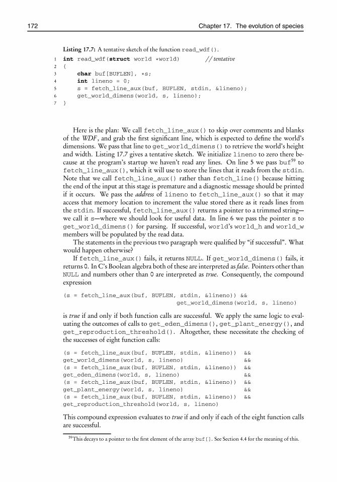
root2014/7/8page 172
�
�
�
�
�
�
�
�
172 Chapter 17. The evolution of species
Listing 17.7: A tentative sketch of the function read_wdf().
1 int read_wdf(struct world *world) // tentative2 {3 char buf[BUFLEN], *s;4 int lineno = 0;5 s = fetch_line_aux(buf, BUFLEN, stdin, &lineno);6 get_world_dimens(world, s, lineno);7 }
Here is the plan: We call fetch_line_aux() to skip over comments and blanksof the WDF , and grab the first significant line, which is expected to define the world’sdimensions. We pass that line to get_world_dimens() to retrieve the world’s heightand width. Listing 17.7 gives a tentative sketch. We initialize lineno to zero there be-cause at the program’s startup we haven’t read any lines. On line 5 we pass buf59 tofetch_line_aux(), which it will use to store the lines that it reads from the stdin.Note that we call fetch_line_aux() rather than fetch_line() because hittingthe end of the input at this stage is premature and a diagnostic message should be printedif it occurs. We pass the address of lineno to fetch_line_aux() so that it mayaccess that memory location to increment the value stored there as it reads lines fromthe stdin. If successful, fetch_line_aux() returns a pointer to a trimmed string—we call it s—where we should look for useful data. In line 6 we pass the pointer s toget_world_dimens() for parsing. If successful, world’s world_h and world_wmembers will be populated by the read data.
The statements in the previous two paragraph were qualified by “if successful”. Whatwould happen otherwise?
If fetch_line_aux() fails, it returns NULL. If get_world_dimens() fails, itreturns 0. In C’s Boolean algebra both of these are interpreted as false. Pointers other thanNULL and numbers other than 0 are interpreted as true. Consequently, the compoundexpression
(s = fetch_line_aux(buf, BUFLEN, stdin, &lineno)) &&get_world_dimens(world, s, lineno)
is true if and only if both function calls are successful. We apply the same logic to eval-uating the outcomes of calls to get_eden_dimens(), get_plant_energy(), andget_reproduction_threshold(). Altogether, these necessitate the checking ofthe successes of eight function calls:
(s = fetch_line_aux(buf, BUFLEN, stdin, &lineno)) &&get_world_dimens(world, s, lineno) &&(s = fetch_line_aux(buf, BUFLEN, stdin, &lineno)) &&get_eden_dimens(world, s, lineno) &&(s = fetch_line_aux(buf, BUFLEN, stdin, &lineno)) &&get_plant_energy(world, s, lineno) &&(s = fetch_line_aux(buf, BUFLEN, stdin, &lineno)) &&get_reproduction_threshold(world, s, lineno)
This compound expression evaluates to true if and only if each of the eight function callsare successful.
59This decays to a pointer to the first element of the array buf[]. See Section 4.4 for the meaning of this.

root2014/7/8page 173
�
�
�
�
�
�
�
�
17.7. The files read.[ch] 173
Listing 17.8: The function read_wdf() in the file read.c. It reads a WDF and return 1 on successand 0 on failure.
1 int read_wdf(struct world *world)2 {3 int animal_count = 0;4 char buf[BUFLEN];5 struct animal *animal;6 int lineno = 0;7 char *s;8
9 int result =10 (s = fetch_line_aux(buf, BUFLEN, stdin, &lineno)) &&11 get_world_dimens(world, s, lineno) &&12 (s = fetch_line_aux(buf, BUFLEN, stdin, &lineno)) &&13 get_eden_dimens(world, s, lineno) &&14 (s = fetch_line_aux(buf, BUFLEN, stdin, &lineno)) &&15 get_plant_energy(world, s, lineno) &&16 (s = fetch_line_aux(buf, BUFLEN, stdin, &lineno)) &&17 get_reproduction_threshold(world, s, lineno);18
19 if (!result)20 return 0;21
22 while ((s = fetch_line(buf, BUFLEN,23 stdin, &lineno)) �= NULL) {24 if ((animal = get_animal_specs(s, lineno)) == NULL)25 return 0;26 else {27 world→herd = ll_push(world→herd, animal);28 animal_count++;29 }30 }31
32 fprintf(stderr, "# %d animal%s read from the input\n",33 animal_count, animal_count == 1 ? "" : "s");34
35 return 1;36 }
The entire function read_wdf() is shown in Listing 17.8. Lines 9 through 17 assignthe value of the compound statement of the eight function calls to the variable result.On line 19 we check the value of result; if it is not true, then at least one of the eightfunction calls has failed. In that case we return from read_wdf() with a status valueof 0 to indicate failure. The calling function will have to deal with the consequences.There is no need to print anything here because each of the eight functions prints its owndiagnostics when an error occurs.
Remark 17.1. Tacit in the logic detailed above is what is known as the short-circuitingproperty of C’s Boolean operators. Specifically, C evaluates compound statements suchas A && B && C && · · · from left to right. It stops the evaluation chain as soon as theoutcome of the overall statement becomes evident. For instance, if A is false, then the
root2014/7/8page 174
�
�
�
�
�
�
�
�
174 Chapter 17. The evolution of species
Listing 17.9: The header file read.h.
1 #ifndef H_READ_H2 #define H_READ_H3 #include "evolution.h"4 int read_wdf(struct world *world);5 #endif /∗ H_READ_H */
entire compound statement is false regardless of the values of B andC; therefore B andC arenot evaluated at all. We often rely on the short-circuiting property in very crucial ways,and what we have in the result = · · · construction is no exception. Note that if the callto the first fetch_line_aux() fails, swill be NULL. If the next expression, that is, thecall to get_world_dimens(), were to be evaluated, the program would crash becausethere is no provision in get_world_dimens() for handling a NULL input. But weneed not be concerned about that since the NULL outcome of the first call short-circuitsthe computation and get_world_dimens() is never called.
Lines 22–30 of read_wdf() handle the animal specification lines. The input mayspecify any number of animals; therefore we process those through a while-loop. Westop when fetch_line() returns NULL, which signals that there is no more data toread. Note that we call fetch_line() rather than fetch_line_aux() becausereaching the end of the input at this stage is normal.
The string fetched on line 22 is passed to get_animal_specs() on line 24. Ifget_animal_specs() returns NULL, it indicates that the string is malformed. Thenwe return from read_wdf() with a status of 0 to indicate failure. Otherwise, we havereceived a pointer to a valid struct animal; therefore on line 27 we call ll_push()to insert that animal in the linked list of animals and then increment animal_count.The animal count does not have a great significance; it’s sent to the stderr on line 32as an information item to reassure the user that the expected number of lines were read.Finally, read_wdf() returns with a status of 1 to indicate the successful completion ofits task.
This completes the description of the file read.c. We add a companion read.h headerfile, shown in Listing 17.9, that presents read.c’s interface. Since the functionread_wdf()is the only one in read.c with external linkage—all others arestatic—thenread_wdf()is the sole function declared in read.h. On line 3 we #include evolution.h since it con-tains the declaration of “struct world”, which is referenced on line 4.
17.8 The files write.[ch]The file write.c defines a function write_wdf() whose purpose is to write a report ofthe current state of the world. The report’s format conforms to the specifications of aWDF , making it possible to use it as input to the evolution simulator for a continuationof the simulation. Listing 17.10 gives an outline of write.c, and Listing 17.11 shows asample report. The report’s top half is produced by simply writing out the informationthat is available in the struct world. The listing of the animals in the bottom half isproduced through a call to the function print_herd() (line 4 of Listing 17.10), whichreceives a pointer to the linked list of animals, walks through the list, and prints the in-formation in each node. To simplify its work, print_herd() delegates the printing ofeach animal line to a helper function, print_animal() (line 3 of Listing 17.10), which
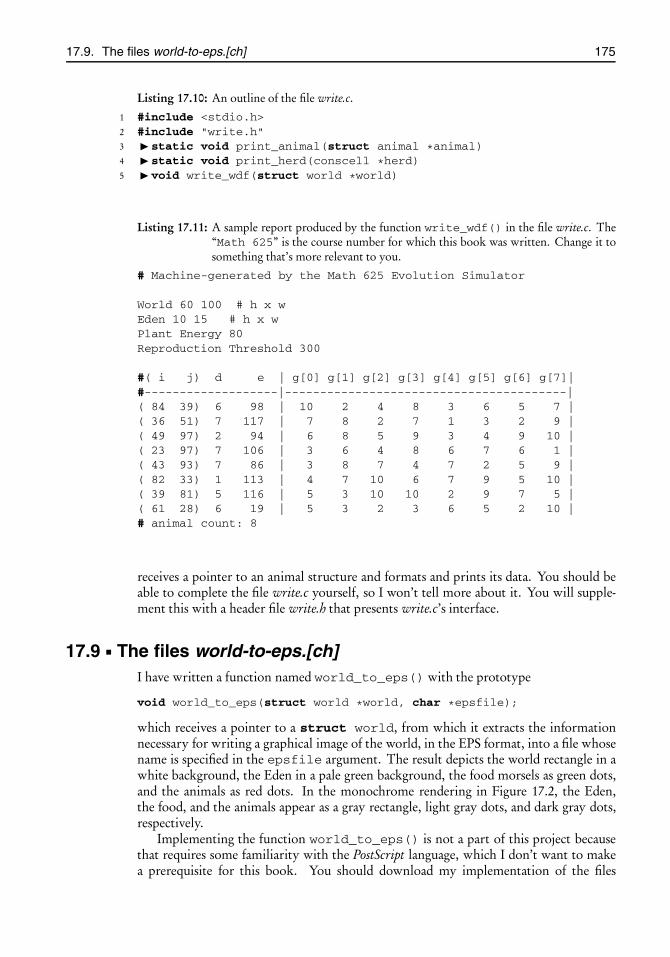
root2014/7/8page 175
�
�
�
�
�
�
�
�
17.9. The files world-to-eps.[ch] 175
Listing 17.10: An outline of the file write.c.
1 #include <stdio.h>2 #include "write.h"3 � static void print_animal(struct animal *animal)4 � static void print_herd(conscell *herd)5 � void write_wdf(struct world *world)
Listing 17.11: A sample report produced by the function write_wdf() in the file write.c. The“Math 625” is the course number for which this book was written. Change it tosomething that’s more relevant to you.
# Machine-generated by the Math 625 Evolution Simulator
World 60 100 # h x wEden 10 15 # h x wPlant Energy 80Reproduction Threshold 300
#( i j) d e | g[0] g[1] g[2] g[3] g[4] g[5] g[6] g[7]|#-------------------|----------------------------------------|( 84 39) 6 98 | 10 2 4 8 3 6 5 7 |( 36 51) 7 117 | 7 8 2 7 1 3 2 9 |( 49 97) 2 94 | 6 8 5 9 3 4 9 10 |( 23 97) 7 106 | 3 6 4 8 6 7 6 1 |( 43 93) 7 86 | 3 8 7 4 7 2 5 9 |( 82 33) 1 113 | 4 7 10 6 7 9 5 10 |( 39 81) 5 116 | 5 3 10 10 2 9 7 5 |( 61 28) 6 19 | 5 3 2 3 6 5 2 10 |# animal count: 8
receives a pointer to an animal structure and formats and prints its data. You should beable to complete the file write.c yourself, so I won’t tell more about it. You will supple-ment this with a header file write.h that presents write.c’s interface.
17.9 The files world-to-eps.[ch]I have written a function named world_to_eps() with the prototype
void world_to_eps(struct world *world, char *epsfile);
which receives a pointer to a struct world, from which it extracts the informationnecessary for writing a graphical image of the world, in the EPS format, into a file whosename is specified in the epsfile argument. The result depicts the world rectangle in awhite background, the Eden in a pale green background, the food morsels as green dots,and the animals as red dots. In the monochrome rendering in Figure 17.2, the Eden,the food, and the animals appear as a gray rectangle, light gray dots, and dark gray dots,respectively.
Implementing the function world_to_eps() is not a part of this project becausethat requires some familiarity with the PostScript language, which I don’t want to makea prerequisite for this book. You should download my implementation of the files

root2014/7/8page 176
�
�
�
�
�
�
�
�
176 Chapter 17. The evolution of species
Figure 17.2: A sample PostScript image produced through the command“./evolution 1000000 1 < world-and-eden.wdf”.The small square near the center is the Eden.
world-to-eps.c and world-to-eps.h from this book’s website, drop them in this project’s di-rectory, and compile them along with the rest of your files.
17.10 Interlude (and a mini-project)We are at about the halfway mark through Project Evolution. It’s a good idea to stop for amoment and test what we have thus far.
Your assignment is to write a program, say interlude.c, that calls read_wdf() to reada WDF from the stdin and then calls write_wdf() to print a report to the stdout.
(a) Compile the program into an executable, say interlude; then run it as
$ ./interlude <world-no-eden.wdf
where world-no-eden.wdf is given in Listing 17.1 on page 166. If all is well, thisshould print out the contents of the input file, minus comments and extra whites-pace, and exit.
(b) Copy world-no-eden.wdf to a temporary file, say tmp.wdf. Insert a few more animalsin it, and try
$ ./interlude <tmp.wdf
(c) Introduce deliberate errors of various sorts in tmp.wdf, and verify that your programcatches them.
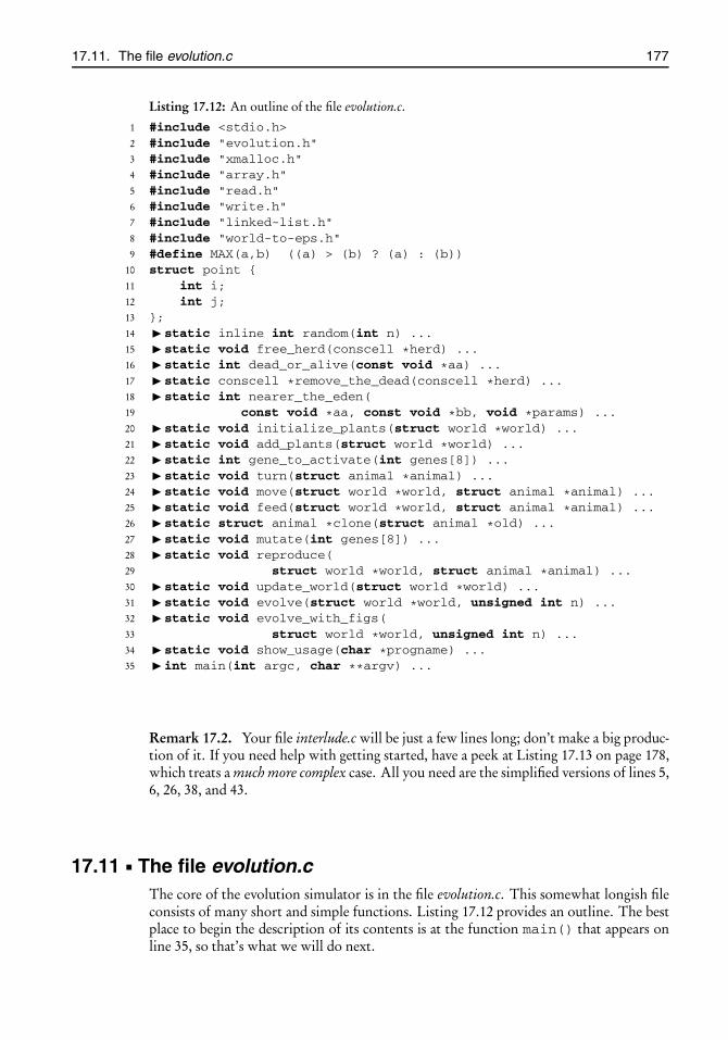
root2014/7/8page 177
�
�
�
�
�
�
�
�
17.11. The file evolution.c 177
Listing 17.12: An outline of the file evolution.c.
1 #include <stdio.h>2 #include "evolution.h"3 #include "xmalloc.h"4 #include "array.h"5 #include "read.h"6 #include "write.h"7 #include "linked-list.h"8 #include "world-to-eps.h"9 #define MAX(a,b) ((a) > (b) ? (a) : (b))
10 struct point {11 int i;12 int j;13 };14 � static inline int random(int n) ...15 � static void free_herd(conscell *herd) ...16 � static int dead_or_alive(const void *aa) ...17 � static conscell *remove_the_dead(conscell *herd) ...18 � static int nearer_the_eden(19 const void *aa, const void *bb, void *params) ...20 � static void initialize_plants(struct world *world) ...21 � static void add_plants(struct world *world) ...22 � static int gene_to_activate(int genes[8]) ...23 � static void turn(struct animal *animal) ...24 � static void move(struct world *world, struct animal *animal) ...25 � static void feed(struct world *world, struct animal *animal) ...26 � static struct animal *clone(struct animal *old) ...27 � static void mutate(int genes[8]) ...28 � static void reproduce(29 struct world *world, struct animal *animal) ...30 � static void update_world(struct world *world) ...31 � static void evolve(struct world *world, unsigned int n) ...32 � static void evolve_with_figs(33 struct world *world, unsigned int n) ...34 � static void show_usage(char *progname) ...35 � int main(int argc, char **argv) ...
Remark 17.2. Your file interlude.c will be just a few lines long; don’t make a big produc-tion of it. If you need help with getting started, have a peek at Listing 17.13 on page 178,which treats a much more complex case. All you need are the simplified versions of lines 5,6, 26, 38, and 43.
17.11 The file evolution.cThe core of the evolution simulator is in the file evolution.c. This somewhat longish fileconsists of many short and simple functions. Listing 17.12 provides an outline. The bestplace to begin the description of its contents is at the function main() that appears online 35, so that’s what we will do next.
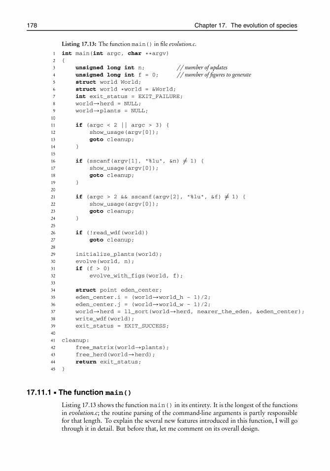
root2014/7/8page 178
�
�
�
�
�
�
�
�
178 Chapter 17. The evolution of species
Listing 17.13: The function main() in file evolution.c.
1 int main(int argc, char **argv)2 {3 unsigned long int n; // number of updates4 unsigned long int f = 0; // number of figures to generate5 struct world World;6 struct world *world = &World;7 int exit_status = EXIT_FAILURE;8 world→herd = NULL;9 world→plants = NULL;
10
11 if (argc < 2 || argc > 3) {12 show_usage(argv[0]);13 goto cleanup;14 }15
16 if (sscanf(argv[1], "%lu", &n) �= 1) {17 show_usage(argv[0]);18 goto cleanup;19 }20
21 if (argc > 2 && sscanf(argv[2], "%lu", &f) �= 1) {22 show_usage(argv[0]);23 goto cleanup;24 }25
26 if (!read_wdf(world))27 goto cleanup;28
29 initialize_plants(world);30 evolve(world, n);31 if (f > 0)32 evolve_with_figs(world, f);33
34 struct point eden_center;35 eden_center.i = (world→world_h - 1)/2;36 eden_center.j = (world→world_w - 1)/2;37 world→herd = ll_sort(world→herd, nearer_the_eden, &eden_center);38 write_wdf(world);39 exit_status = EXIT_SUCCESS;40
41 cleanup:42 free_matrix(world→plants);43 free_herd(world→herd);44 return exit_status;45 }
17.11.1 The function main()
Listing 17.13 shows the function main() in its entirety. It is the longest of the functionsin evolution.c; the routine parsing of the command-line arguments is partly responsiblefor that length. To explain the several new features introduced in this function, I will gothrough it in detail. But before that, let me comment on its overall design.

root2014/7/8page 179
�
�
�
�
�
�
�
�
17.11. The file evolution.c 179
The execution of the function main() may have to be halted at various points due topossible faulty data submitted by the user. For instance, the user may have given illegalcommand-line arguments, or perhaps the WDF is incomplete or garbled. Whenever anysuch error is encountered within main(), the program’s flow jumps via a goto to thecleanup label on line 41, subsequent to which the memory resources are freed and theprogram terminates with the exit status assigned to a variable named exit_status,60
which is assigned the default value of EXIT_FAILURE on line 7. Only when the programnears the completion of its mission on line 39 is its value changed to EXIT_SUCCESS.
Here we begin the line by line analysis of the function main():
Line 1: We invoke main() with the argc and argv parameters because we intend tocapture the command-line arguments. Here you will need the information fromSection 4.7 on the details of how the command-line arguments are stored in mem-ory.
Lines 3 and 4: The user specifies the number of iterations and the number of snapshotson the command-line. The former is required; the latter is optional. Further down,where we parse the command-line arguments, we store those numbers in the vari-ables n and f, respectively. We set f to zero here as its default value.
Line 5: The World defined here is a struct worldwhich is to hold the complete datathat characterizes the world at every instant. Most of our program’s functions needaccess to that data to perform their tasks. It suffices to pass World’s address to suchfunctions. They will query the structure for data through that address, and evenmodify that data if they are supposed to.
Line 6: We define the auxiliary variable world (with lowercase w) to hold World’s ad-dress. This is by no means essential since we may equally well use &World forWorld’s address. There is a slight drawback to that, however. Within main() wehave access to both World and its address, &World. Outside of main() we haveaccess only to World’s address. Working with World in main() and World’saddress outside main() results in a certain cognitive dissonance that we wish toavoid. That’s why we work with world instead of &World in the rest of main().
Line 7: Upon exit, the program will return the value of exit_status to the callingenvironment. We set exit_status toEXIT_FAILURE as its default value. Onlyif all is well will we change it to EXIT_SUCCESS.
Lines 8 and 9: The world→herd points to the head of the linked list of animals. Weset it to NULL here to indicate that initially the linked list is empty.
The world→plants is going to point to a world_h × world_w matrix (to beallocated later) whose (i , j ) entry holds the number of plants in cell (i , j ). We set itto NULL here for a different, and a more subtle, reason.
In several places in main() where we encounter unacceptable situations, webail out through a “goto cleanup”, which makes the execution jump to thecleanup label where free_matrix(world→plants) is called, among otherthings, to free the memory associated with the plants matrix. If we omit line 9,then world→plantswill have an undetermined (junk) value; therefore the call tofree_matrix(world→plants) is likely to crash the program. On the other
60There is nothing special about the name “exit_status”. I called it that because it expresses its intentwell.
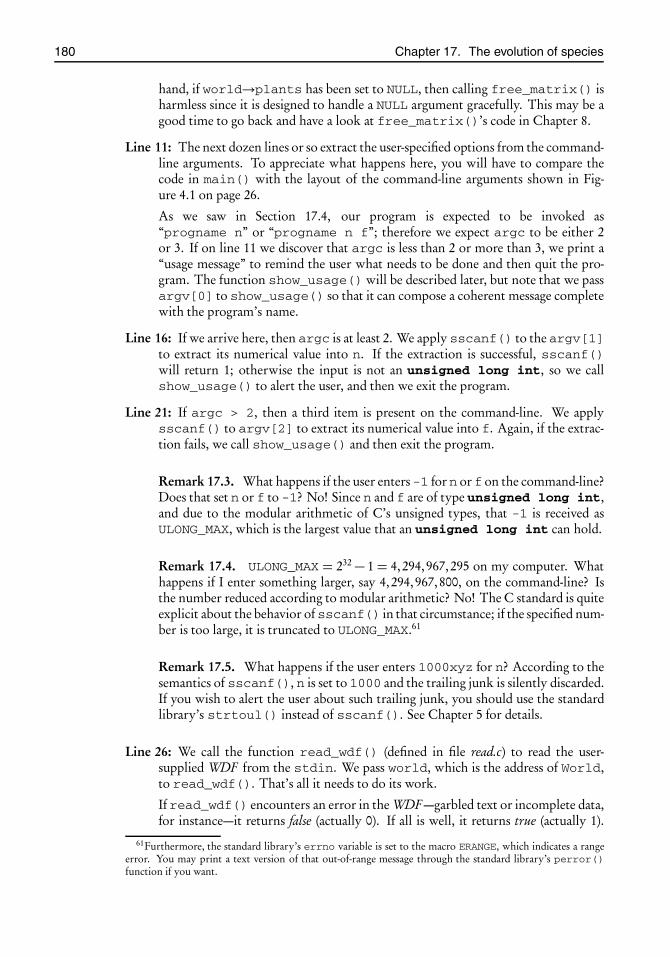
root2014/7/8page 180
�
�
�
�
�
�
�
�
180 Chapter 17. The evolution of species
hand, if world→plants has been set to NULL, then calling free_matrix() isharmless since it is designed to handle a NULL argument gracefully. This may be agood time to go back and have a look at free_matrix()’s code in Chapter 8.
Line 11: The next dozen lines or so extract the user-specified options from the command-line arguments. To appreciate what happens here, you will have to compare thecode in main() with the layout of the command-line arguments shown in Fig-ure 4.1 on page 26.
As we saw in Section 17.4, our program is expected to be invoked as“progname n” or “progname n f”; therefore we expect argc to be either 2or 3. If on line 11 we discover that argc is less than 2 or more than 3, we print a“usage message” to remind the user what needs to be done and then quit the pro-gram. The function show_usage() will be described later, but note that we passargv[0] to show_usage() so that it can compose a coherent message completewith the program’s name.
Line 16: If we arrive here, then argc is at least 2. We apply sscanf() to the argv[1]to extract its numerical value into n. If the extraction is successful, sscanf()will return 1; otherwise the input is not an unsigned long int, so we callshow_usage() to alert the user, and then we exit the program.
Line 21: If argc > 2, then a third item is present on the command-line. We applysscanf() to argv[2] to extract its numerical value into f. Again, if the extrac-tion fails, we call show_usage() and then exit the program.
Remark 17.3. What happens if the user enters -1 for n or f on the command-line?Does that set n or f to -1? No! Since n and f are of type unsigned long int,and due to the modular arithmetic of C’s unsigned types, that -1 is received asULONG_MAX, which is the largest value that an unsigned long int can hold.
Remark 17.4. ULONG_MAX = 232 − 1 = 4,294,967,295 on my computer. Whathappens if I enter something larger, say 4,294,967,800, on the command-line? Isthe number reduced according to modular arithmetic? No! The C standard is quiteexplicit about the behavior of sscanf() in that circumstance; if the specified num-ber is too large, it is truncated to ULONG_MAX.61
Remark 17.5. What happens if the user enters 1000xyz for n? According to thesemantics of sscanf(), n is set to 1000 and the trailing junk is silently discarded.If you wish to alert the user about such trailing junk, you should use the standardlibrary’s strtoul() instead of sscanf(). See Chapter 5 for details.
Line 26: We call the function read_wdf() (defined in file read.c) to read the user-supplied WDF from the stdin. We pass world, which is the address of World,to read_wdf(). That’s all it needs to do its work.
If read_wdf() encounters an error in the WDF —garbled text or incomplete data,for instance—it returns false (actually 0). If all is well, it returns true (actually 1).
61Furthermore, the standard library’s errno variable is set to the macro ERANGE, which indicates a rangeerror. You may print a text version of that out-of-range message through the standard library’s perror()function if you want.
root2014/7/8page 181
�
�
�
�
�
�
�
�
17.11. The file evolution.c 181
On line 26 we check the return value. If it’s other than true, we jump to cleanupand therefore exit the program. No message is printed here because read_wdf()itself prints diagnostics as it encounters problems.
Line: 29: The function initialize_plants() allocates memory for the matrix ofplants and sets all its elements to zero. The world begins with no plants at all.
Line: 30: This is where the real action takes place—evolve(world, n) takes the worldthrough n time-steps.
Line 31: If f is nonzero, then the program takes f graphical snapshots of the world,interleaving world updates with snapshots.
Lines 34–37: We define eden_center according to the formula (17.3) on page 164. Thestruct point structure that occurs on line 34 is declared on line 10 in List-ing 17.12. We call ll_sort() to sort the linked list of the animals accordingto increasing distance from eden_center. Thus, animals nearer the Eden willcome first in the list, and a listing of the herd should reveal genetic differences, ifany, between the animals near and far from the Eden. The comparison function,nearer_the_eden(), that appears as an argument to ll_sort() on line 37 isdescribed in subsection 17.11.6 on page 182.
Remark 17.6. The placement of the declaration of eden_center on line 34assumes C99. To revert to C89, move that declaration to the top of main() sinceC89 requires all declarations to precede executable statements in a block.
Line 38: We write the world’s current data in the WDF format to the stdout.
At this point the program has accomplished its mission; therefore on the next linewe change the value of exit_status to EXIT_SUCCESS.
Line 41: The cleanup label has been the jumping target from many places throughoutmain(). There is not much to do once we arrive here. We free the memory re-sources and return from main()—and consequently exit the program—with thestatus of exit_status, which has been set earlier to one of EXIT_SUCCESS orEXIT_FAILURE.
This completes the description of the somewhat longish function main(). In com-parison, the remaining functions in evolution.c are shorter and simpler. We set out todescribe those next.
17.11.2 The function show_usage()
The function show_usage() that appears on line 34 in Listing 17.12 on page 177 printsa brief help message on the program’s usage. It is invoked from several places in main()(in Listing 17.13) wherever the user’s input disagrees with the program’s expectations.I will not give an outline; you write the whole thing. My version prints
Usage: ./evolution n [f] <infile >outfilen ≥ 0 : (required) number of updatesf ≥ 0 : (optional) number of snapshots after n updatesReads World Definition from infile, performsn updates, and writes result to outfile

root2014/7/8page 182
�
�
�
�
�
�
�
�
182 Chapter 17. The evolution of species
Remark 17.7. The program’s name arrives as an argument to show_usage(). Usethat; don’t hard-code the program’s name into the function’s body.
Remark 17.8. On the “Usage” line I have placed f in square brackets. That’s the tradi-tional way—at least in the Unix world—of indicating that the argument is optional.
17.11.3 The function random()
The function random() that appears on line 14 in Listing 17.12 on page 177 is exactlythe function random() of Listing 10.1 on page 73 in Chapter 10. Just copy the codefrom there into your evolution.c.
17.11.4 The function free_herd()
The function free_herd() that appears on line 15 in Listing 17.12 on page 177 freesthe memory resources associated with a linked list of animals. Note that the functionll_free() developed in Chapter 16 merely frees the memory of a linked list’s conscells. It does not touch the data that the cons cells point to. Freeing the linked list ofanimals, therefore, requires two passes, first to free the data and then to free the cons cells,as in
1 static void free_herd(conscell *herd)2 {3 for (conscell *p = herd; p �= NULL; p = p→next)4 free(p→data);5 ll_free(herd);6 }
17.11.5 The functions dead_or_alive() and remove_the_dead()
After each time-step, the program scans the linked list of the animals and removes thedead. An animal is dead if its energy has dropped to zero or below. The functiondead_or_alive() that appears on line 16 in Listing 17.12 on page 177 receives apointer to an animal and returns true or false (that is, 1 or 0) depending on whether theanimal is alive or dead, respectively. I will leave it to you to implement that function.
The function remove_the_dead() that appears on line 17 in Listing 17.12 is asimple wrapper around Chapter 16’s ll_filter() function to cull the herd. Here it isin its entirety:
1 static conscell *remove_the_dead(conscell *herd)2 {3 conscell *dead = NULL;4 herd = ll_filter(herd, dead_or_alive, &dead);5 free_herd(dead);6 return herd;7 }
Be sure to understand how it works, and then add it to your evolution.c.
17.11.6 The function nearer_the_eden()
The most striking and significant finding of this simulated evolution is that in the presenceof the Eden, the animals evolve into two distinct species: those who live in or near the
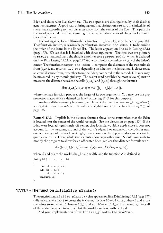
root2014/7/8page 183
�
�
�
�
�
�
�
�
17.11. The file evolution.c 183
Eden and those who live elsewhere. The two species are distinguished by their distinctgenetic structures. A good way of bringing out that distinction is to sort the linked list ofthe animals according to their distances away from the center of the Eden. This puts thespecies of one kind near the beginning of the list and the species of the other kind nearthe end of the list.
The sorting is performed through the functionll_sort(), as explained on page 181.That function, in turn, relies on a helper function, nearer_the_eden(), to determinethe order of the items in the linked list. The latter appears on line 18 in Listing 17.12(page 177). We see that it is invoked with three arguments. The first two are pointersto struct animal, and the third is a pointer to a struct point, which is declaredon line 10 in Listing 17.12 on page 177 and which holds the indices (ei , e j ) of the Eden’scenter. The function nearer_the_eden() computes the distances of the two animalsfrom (ei , e j ), and returns -1, 0, or 1 depending on whether the first animal is closer to, atan equal distance from, or farther from the Eden, compared to the second. Distance maybe measured in any meaningful way. The easiest (and possibly the most relevant) metricmeasures the distance between the cells (ai ,aj ) and (ei , e j ) through the formula
dist�(ai ,aj ), (ei , e j )
=max
�|ai − ei |, |aj − e j | ,
where the max function produces the larger of its two arguments. You may use the pre-processor macro MAX() defined on line 9 of Listing 17.12 for this purpose.
You have all the necessary bits now to implement the functionnearer_the_eden()and add it to your evolution.c. It will be a slight variant of the function cmp2() ofpage 155.
Remark 17.9. Implicit in the distance formula above is the assumption that the Edenis located near the center of the world rectangle. (See the discussion on page 163.) If theEden were located significantly off center, that formula wouldn’t apply since it does notaccount for the wrapping around of the world’s edges. For instance, if the Eden is nearone of the edges of the world rectangle, then a point on the opposite edge can be actuallyquite close to the Eden, while the formula above says otherwise. Should you wish tomodify the program to allow for an off-center Eden, replace that distance formula with
dist�(ai ,aj ), (ei , e j )
=max
�φ(ai − ei , h),φ(aj − e j , w)
,
where h and w are the world’s height and width, and the function φ is defined as
int phi(int x, int L){
int d = abs(x);if (d > L/2)
d = L - d;return d;
}
17.11.7 The function initialize_plants()
The functioninitialize_plants() that appears on line 20 in Listing 17.12 (page 177)calls make_matrix() to create the h×w matrix world→plants, where h and w arethe values stored in world→world_h and world→world_w. Furthermore, it sets allof the matrix’s entries to zero so that the world starts out with no food.
Add your implementation of initialize_plants() to evolution.c.

root2014/7/8page 184
�
�
�
�
�
�
�
�
184 Chapter 17. The evolution of species
Listing 17.14: An outline of the function add_plants() in the file evolution.c.
1 static void add_plants(struct world *world)2 {3 int i = random(world→world_h);4 int j = random(world→world_w);5 world→plants[i][j]++;6
7 if (world→eden_h > 0 && world→eden_w > 0) {8 i = ... �9 j = ... �
10 world→plants[i][j]++;11 }12 }
17.11.8 The function add_plants()
The function add_plants() that appears on line 21 in Listing 17.12 on page 177 isexecuted once at the beginning of every time-step. It is responsible for depositing onemorsel of food in a random cell in the world and another morsel of food in a random cellin the Eden, if an Eden exists.
Listing 17.14 shows an outline. On lines 3 and 4 we pick random numbers i and jin the ranges {0,1, . . . , h − 1} and {0,1, . . . , w − 1}, where h and w are the dimensionsof the world, that is, world→world_h and world→world_w. Consequently, (i , j )represents a random cell in the world. Incrementing world→plants[i][j] on line 5amounts to depositing a morsel of food there.
The purpose of the function’s second half is to deposit an additional morsel of food inthe Eden. You should be able to fill the excised parts with the help of the formula (17.2)on page 164.
17.11.9 The function gene_to_activate()
The functiongene_to_activate() that appears on line 22 in Listing 17.12 on page 177receives a chromosome, i.e., an array of eight genes, ⟨g0, g1, . . . , g7⟩, and selects a randomgene to activate. It returns the index (i.e., a number in the set {0,1, . . . , 7}) of the selectedgene.
If we were to select any of the genes with equal probability, then it would have beena matter of calling random(8) to get the desired index. But our task is a bit more com-plicated; we wish to assign higher probability of selection to genes of larger values. Theway to do this is to consider eight line segments of lengths gk for k = 0,1, . . . , 7. Lay themback-to-back, and in order, from left to right, to obtain a line segment of overall lengthL =
∑7k=0 gk . Figure 17.3 shows this for the chromosome ⟨2,4,1,1,6,3,1,2⟩, which has
L= 20.Pick a random number r with uniform distribution in the range {0,1, . . . , L−1}. (Let-
ting r = random(L) will do that.) The key observation is that such a number is morelikely to fall on a longer segment than a short one.
The outcome r = 9, for instance, falls on the segment corresponding to the gene g4,as seen in Figure 17.3. In that case gene_to_activate() will return 4 to signal thatthe gene g4 is to be activated.
How does gene_to_activate() know that r = 9 falls on the interval g4? It seesthat r − (g0 + g1+ g2+ g3)> 0 but r − (g0+ g1 + g2+ g3 + g4)< 0. That’s how.
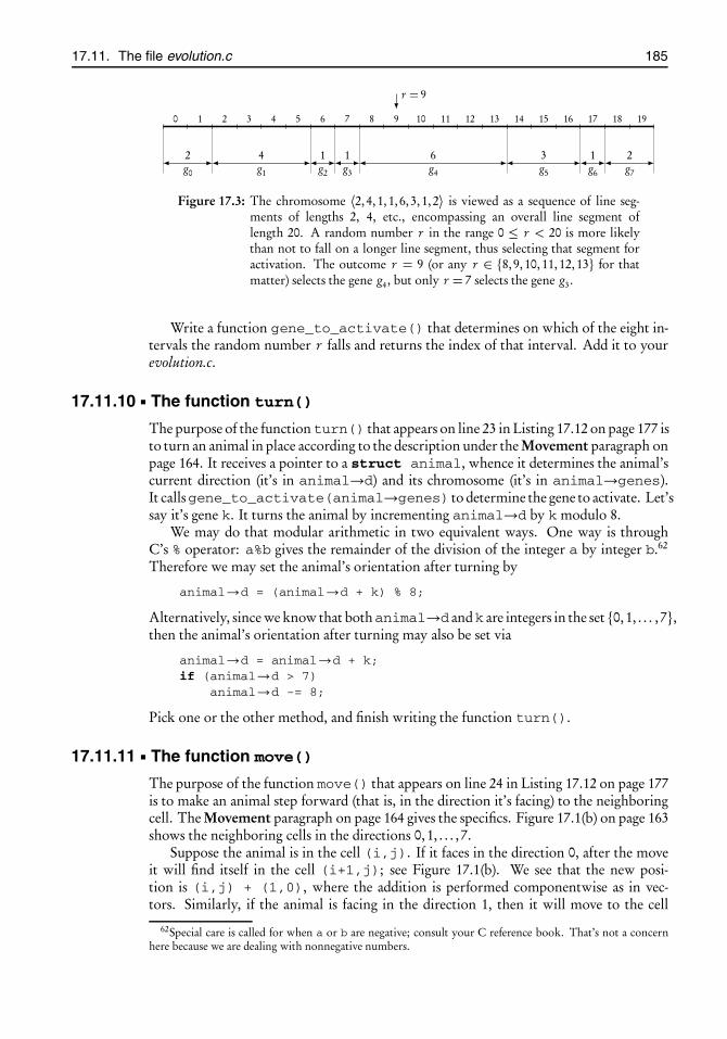
root2014/7/8page 185
�
�
�
�
�
�
�
�
17.11. The file evolution.c 185
0 1 2 3 4 5 6 7 8 9 10 11 12 13 14 15 16 17 18 19
r = 9
g0
2g1
4g2
1g3
1g4
6g5
3g6
1g7
2
Figure 17.3: The chromosome ⟨2,4,1,1,6,3,1,2⟩ is viewed as a sequence of line seg-ments of lengths 2, 4, etc., encompassing an overall line segment oflength 20. A random number r in the range 0 ≤ r < 20 is more likelythan not to fall on a longer line segment, thus selecting that segment foractivation. The outcome r = 9 (or any r ∈ {8,9,10,11,12,13} for thatmatter) selects the gene g4, but only r = 7 selects the gene g3.
Write a function gene_to_activate() that determines on which of the eight in-tervals the random number r falls and returns the index of that interval. Add it to yourevolution.c.
17.11.10 The function turn()
The purpose of the functionturn() that appears on line 23 in Listing 17.12 on page 177 isto turn an animal in place according to the description under the Movement paragraph onpage 164. It receives a pointer to a struct animal, whence it determines the animal’scurrent direction (it’s in animal→d) and its chromosome (it’s in animal→genes).It callsgene_to_activate(animal→genes) to determine the gene to activate. Let’ssay it’s gene k. It turns the animal by incrementing animal→d by k modulo 8.
We may do that modular arithmetic in two equivalent ways. One way is throughC’s % operator: a%b gives the remainder of the division of the integer a by integer b.62
Therefore we may set the animal’s orientation after turning by
animal→d = (animal→d + k) % 8;
Alternatively, since we know that bothanimal→d andk are integers in the set {0,1, . . . , 7},then the animal’s orientation after turning may also be set via
animal→d = animal→d + k;if (animal→d > 7)
animal→d -= 8;
Pick one or the other method, and finish writing the function turn().
17.11.11 The function move()
The purpose of the function move() that appears on line 24 in Listing 17.12 on page 177is to make an animal step forward (that is, in the direction it’s facing) to the neighboringcell. The Movement paragraph on page 164 gives the specifics. Figure 17.1(b) on page 163shows the neighboring cells in the directions 0,1, . . . , 7.
Suppose the animal is in the cell (i,j). If it faces in the direction 0, after the moveit will find itself in the cell (i+1,j); see Figure 17.1(b). We see that the new posi-tion is (i,j) + (1,0), where the addition is performed componentwise as in vec-tors. Similarly, if the animal is facing in the direction 1, then it will move to the cell
62Special care is called for when a or b are negative; consult your C reference book. That’s not a concernhere because we are dealing with nonnegative numbers.
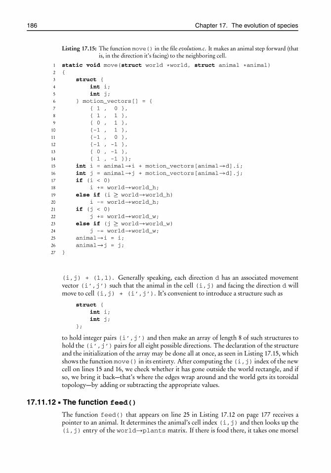
root2014/7/8page 186
�
�
�
�
�
�
�
�
186 Chapter 17. The evolution of species
Listing 17.15: The function move() in the file evolution.c. It makes an animal step forward (thatis, in the direction it’s facing) to the neighboring cell.
1 static void move(struct world *world, struct animal *animal)2 {3 struct {4 int i;5 int j;6 } motion_vectors[] = {7 { 1 , 0 },8 { 1 , 1 },9 { 0 , 1 },
10 {-1 , 1 },11 {-1 , 0 },12 {-1 , -1 },13 { 0 , -1 },14 { 1 , -1 }};15 int i = animal→i + motion_vectors[animal→d].i;16 int j = animal→j + motion_vectors[animal→d].j;17 if (i < 0)18 i += world→world_h;19 else if (i ≥ world→world_h)20 i -= world→world_h;21 if (j < 0)22 j += world→world_w;23 else if (j ≥ world→world_w)24 j -= world→world_w;25 animal→i = i;26 animal→j = j;27 }
(i,j) + (1,1). Generally speaking, each direction d has an associated movementvector (i’,j’) such that the animal in the cell (i,j) and facing the direction d willmove to cell (i,j) + (i’,j’). It’s convenient to introduce a structure such as
struct {int i;int j;
};
to hold integer pairs (i’,j’) and then make an array of length 8 of such structures tohold the (i’,j’) pairs for all eight possible directions. The declaration of the structureand the initialization of the array may be done all at once, as seen in Listing 17.15, whichshows the function move() in its entirety. After computing the (i,j) index of the newcell on lines 15 and 16, we check whether it has gone outside the world rectangle, and ifso, we bring it back—that’s where the edges wrap around and the world gets its toroidaltopology—by adding or subtracting the appropriate values.
17.11.12 The function feed()
The function feed() that appears on line 25 in Listing 17.12 on page 177 receives apointer to an animal. It determines the animal’s cell index (i,j) and then looks up the(i,j) entry of the world→plants matrix. If there is food there, it takes one morsel

root2014/7/8page 187
�
�
�
�
�
�
�
�
17.11. The file evolution.c 187
and feeds it to the animal. The food count in the cell drops by one and the animal’s energyincreases by world→plant_energy. That’s all. You should be able to do the details.
17.11.13 The function clone()
The function clone() that appears on line 26 in Listing 17.12 on page 177 receives apointer to an animal. It creates an identical animal and returns a pointer to it. The func-tion is quite straightforward. It calls xmalloc() as in
struct animal *new = xmalloc(sizeof *new);
to allocate memory for the clone and then copies all the data from the original to theclone. You should be able to do the details.
17.11.14 The function mutate()
The function mutate() that appears on line 27 in Listing 17.12 on page 177 receives apointer to a chromosome and mutates it in the way described under the headingMutation on page 165. Its implementation is quite straightforward, so I will leave thework to you, but here are two hints.
First, observe that random(3) returns a random integer in the set {0,1,2}; thereforerandom(3)-1 is a random integer in the set {−1,0,1}. Second, you may have use forthe preprocessor macro MAX() defined on line 9 in Listing 17.12, which finds the largerof its two arguments.
17.11.15 The function reproduce()
The function reproduce() that appears on line 28 in Listing 17.12 on page 177 receivesa pointer to an animal and splits it in two. Specifically, it cuts down the animal’s energy tohalf, callsclone() to make an exact copy, calls mutate() to mutate the cloned animal’schromosome, and then pushes the cloned animal into the linked list of the animals. Hereis that function in its entirety:
1 static void reproduce(struct world *world, struct animal *animal)2 {3 animal→e /= 2;4 struct animal *new = clone(animal);5 mutate(new→genes);6 world→herd = ll_push(world→herd, new);7 }
Examine the code carefully, and especially note how ll_push() is used. When you feelcomfortable with your understanding, insert the function in your evolution.c.
17.11.16 The function update_world()
The function update_world() that appears on line 30 in Listing 17.12 on page 177updates the world by one time-step. It sees to it that (a) dead animals are removed fromthe linked list of animals; (b) each of the remaining animals turns and then moves to anadjacent cell, eats food if there is any, and reproduces if it has sufficient energy; and (c) addsa plant somewhere in the world, and another one somewhere in the Eden, if there is anEden. Listing 17.16 shows my implementation. As always, go through it carefully andanalyze every piece. Then insert it into your evolution.c.
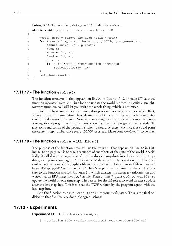
root2014/7/8page 188
�
�
�
�
�
�
�
�
188 Chapter 17. The evolution of species
Listing 17.16: The function update_world() in the file evolution.c.
1 static void update_world(struct world *world)2 {3 world→herd = remove_the_dead(world→herd);4 for (conscell *p = world→herd; p �= NULL; p = p→next) {5 struct animal *a = p→data;6 turn(a);7 move(world, a);8 feed(world, a);9 a→e--;
10 if (a→e ≥ world→reproduction_threshold)11 reproduce(world, a);12 }13 add_plants(world);14 }
17.11.17 The function evolve()
The function evolve() that appears on line 31 in Listing 17.12 on page 177 calls thefunction update_world() in a loop to update the world n times. It’s quite a straight-forward function, so I will let you write the whole thing, which is not much.
Evolution by its nature is an extremely slow process. To achieve any discernible effect,we need to run the simulation through millions of time-steps. Even on a fast computerthis may take several minutes. Now, it is annoying to stare at a silent computer screenwaiting for the program to finish and not knowing how much progress is being made. Togive some indication of the program’s state, it would be extremely nice if it could printthe current step number once every 100,000 steps, say. Make your evolve() to do that.
17.11.18 The function evolve_with_figs()
The purpose of the function evolve_with_figs() that appears on line 32 in List-ing 17.12 on page 177 is to take a sequence of snapshots of the state of the world. Specif-ically, if called with an argument of n, it produces n snapshots interleaved with n-1 up-dates, as explained on page 167. Listing 17.17 shows an implementation. On line 5 wesynthesize the name of the graphics file in the array buf. The sequence of file names willbe fig0000.eps, fig0001.eps, and so on. On line 6 we pass the file name and the world struc-ture to the function world_to_eps(), which extracts the necessary information andwrites it as an EPS image into a fig*.eps file. Then on line 8 it calls update_world() toupdate the world by one time-step. The reason for the if-test is to avoid an extra updateafter the last snapshot. This is so that the WDF written by the program agrees with thelast snapshot.
Add the function evolve_with_figs() to your evolution.c. This is the final ad-dition to that file. You are done. Congratulations!
17.12 ExperimentsExperiment #1: For the first experiment, try
$ ./evolution 1000 <world-no-eden.wdf >out-no-eden-1000.wdf
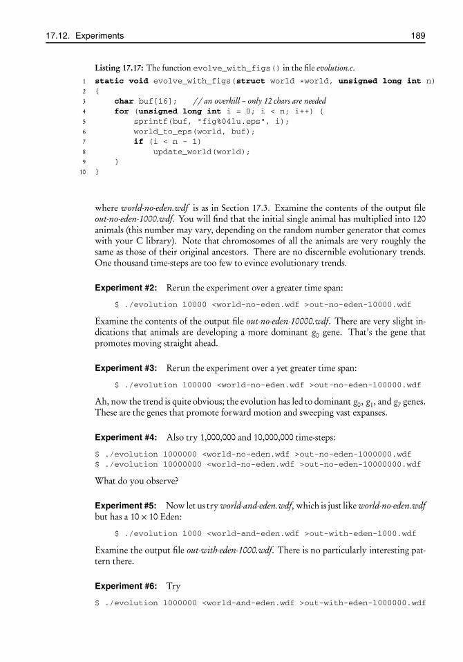
root2014/7/8page 189
�
�
�
�
�
�
�
�
17.12. Experiments 189
Listing 17.17: The function evolve_with_figs() in the file evolution.c.
1 static void evolve_with_figs(struct world *world, unsigned long int n)2 {3 char buf[16]; // an overkill – only 12 chars are needed4 for (unsigned long int i = 0; i < n; i++) {5 sprintf(buf, "fig%04lu.eps", i);6 world_to_eps(world, buf);7 if (i < n - 1)8 update_world(world);9 }
10 }
where world-no-eden.wdf is as in Section 17.3. Examine the contents of the output fileout-no-eden-1000.wdf. You will find that the initial single animal has multiplied into 120animals (this number may vary, depending on the random number generator that comeswith your C library). Note that chromosomes of all the animals are very roughly thesame as those of their original ancestors. There are no discernible evolutionary trends.One thousand time-steps are too few to evince evolutionary trends.
Experiment #2: Rerun the experiment over a greater time span:
$ ./evolution 10000 <world-no-eden.wdf >out-no-eden-10000.wdf
Examine the contents of the output file out-no-eden-10000.wdf. There are very slight in-dications that animals are developing a more dominant g0 gene. That’s the gene thatpromotes moving straight ahead.
Experiment #3: Rerun the experiment over a yet greater time span:
$ ./evolution 100000 <world-no-eden.wdf >out-no-eden-100000.wdf
Ah, now the trend is quite obvious; the evolution has led to dominant g0, g1, and g7 genes.These are the genes that promote forward motion and sweeping vast expanses.
Experiment #4: Also try 1,000,000 and 10,000,000 time-steps:
$ ./evolution 1000000 <world-no-eden.wdf >out-no-eden-1000000.wdf$ ./evolution 10000000 <world-no-eden.wdf >out-no-eden-10000000.wdf
What do you observe?
Experiment #5: Now let us try world-and-eden.wdf, which is just like world-no-eden.wdfbut has a 10× 10 Eden:
$ ./evolution 1000 <world-and-eden.wdf >out-with-eden-1000.wdf
Examine the output file out-with-eden-1000.wdf. There is no particularly interesting pat-tern there.
Experiment #6: Try
$ ./evolution 1000000 <world-and-eden.wdf >out-with-eden-1000000.wdf

root2014/7/8page 190
�
�
�
�
�
�
�
�
190 Chapter 17. The evolution of species
Examine the output file out-with-eden-1000000.wdf. Do you see that there are two distinctspecies now? Recall that the program sorts the animals according to their distances awayfrom the Eden.
Experiment #7: Also try
$ ./evolution 10000000 <world-and-eden.wdf >out-with-eden-10000000.wdf
The two distinct species stand out even more clearly now. Do you see the foreign speciesstreaking through the Eden?
17.13 AnimationTry
$ ./evolution 100000 20 <world-and-eden.wdf >/dev/null
This runs the evolution for an initial 100,000 steps; then it takes 20 snapshots inter-leaved with updates. The snapshots are stored in the EPS files named fig0000.eps throughfig0019.eps. Figure 17.2 on page 176 shows a sample snapshot.
The /dev/null that appears in the command above is Unix’s “black hole”; any streamdirected to it just vanishes. I am redirecting the program’s stdout stream to /dev/nullsince I am not interested in seeing the WDF file that it writes—I have seen it already inthe previous section’s experiments.
How do we view the snapshots? There are many ways, but these depend very muchon your computer’s operating system. I can tell you what I use on Linux. You will haveto find out what is available to you if your operating system is different.
• You may view the individual snapshots through any PostScript image viewer. Theprograms display, evince, and gv are among the many such utilities freelyavailable on Linux platforms. I prefer evince for viewing single frames:
$ evince fig0007.eps
• The display utility noted above is a part of the ImageMagick suite of image view-ing and manipulation programs. The suite also contains theanimate utility, whichanimates a sequence of images. Try
$ animate -delay 25 fig*.eps
You will have to give it a few seconds at startup since it has to read and digest all theframes ahead of time. Then it will show the 20 images in quick succession, as in amovie, and will loop forever. To stop the animation, move the mouse cursor insidethe animation window and press the keyboard’s “q” key.The-delay 25 option makes the animation pause for 25/100 of a second betweenframes. Adjust it for slower or faster playback.
• I prefer more control in an animation. I like to stop it where I want to and moveforward or backward one frame at a time. For that, see if you have the feh imageviewing utility on your computer. It comes with most Linux distributions. Youmay also download the source for free from <http://feh.finalrewind.org/>
and compile it yourself.Feh does not recognize PostScript. You will have to convert the fig*.eps files to araster-based image format, such as PNG. This may be done through the convertutility that comes with ImageMagick:
$ convert fig*.eps fig%04d.png

root2014/7/8page 191
�
�
�
�
�
�
�
�
17.14. Project Evolution 191
Within a few seconds, this will convert the PostScript files fig0000.eps throughfig0019.eps to PNG images fig0000.png through fig0019.png. The %04d specifies4-digit, zero-filled numbering of the output files. View the resulting images with
$ feh fig*.png
Press the keyboard’s right and left arrows to move forward and backward throughthe images. Or just hold down one of those keys to let feh flip through those imagesas fast as it can, thus creating the illusion of an animation.
You will find a GIF animation in the book’s website. I made that by packing a se-quence of individual snapshots into an animated GIF file. Read the website to learn howit is done.
17.14 Project Evolution
Part 17.1. Complete and test the mini-project of Section 17.10.
Part 17.2. Run the experiments suggested in Sections 17.12 and 17.13. Then change theparameters in the WDF s and try again. Is evolution always successful?
Part 17.3. [optional] Entering large numbers such as 10000000 on the command-lineis inconvenient because you have to carefully count the zeros. Modify the program’scommand-line parsing section to make it recognize the K, M, G suffixes63 for numbers.Thus, 10K would mean ten thousand, 15M would mean 15 million, and 2G would mean2 billion.
Part 17.4. [optional] The WDF defined in Section 17.3 carries no information about thedistribution of food in the world. That’s why our simulation begins with zero food. Seeif you can extend the definition of WDF to handle a prescribed food distribution. Youmay consider a syntax like
Food (i0,j0,n0) (i1,j1,n1) ...
to indicate that the cell (i0, j0) has n0 morsels of food, etc. You will need to modify thefunctions read_wdf() and write_wdf() to handle such a specification.
This extension increases the program’s versatility significantly since the WDF writtenby write_wdf() now contains the simulation’s complete state upon the program’s exit.That WDF then may be used as input to the program to continue the simulation whereit was left off.
Part 17.5. [optional] Write a one-dimensional version of the evolution simulator. Theworld would be a line interval whose ends are identified; i.e., an animal exiting at one endemerges at the other end. (Topologically the world would be a circle.) The chromosomewill consist of two genes ⟨g0, g1⟩. If g0 is activated, the animal will not turn. If g1 isactivated, it will do an about-face.
63These are the first letters of Kilo, Mega, and Giga, which correspond to multiplicative factors of 103, 106,and 109, respectively.
root2014/7/8page 193
�
�
�
�
�
�
�
�
Chapter 18
The Nelder–Meaddownhill simplex
Prerequisites: Chapters 7, 8
18.1 IntroductionThe Nelder–Mead simplex method [49, 50] is an algorithm for finding the local minimaof a function f : Rn →R, called the objective function in optimization parlance. The ideabehind it is very geometric. It starts with a suitably chosen initial simplex64 in Rn andevolves it according to certain rules. The simplex undergoes iterative expansions, contrac-tions, and displacements, and if everything goes according to plan, it moves “downhill”toward a local minimum of f . The term “downhill simplex” was used in [53] to refer tothis behavior. A significant merit of the algorithm is that it is gradient-free, that is, it doesnot require a knowledge of the function’s gradient, which may be difficult or expensiveto compute. Consequently, it may be applied to minimize nondifferentiable functions,but see the caveats in Section 18.3.
18.2 The algorithmThe algorithm works in iterative cycles. I will explain what is done in one cycle. Thecycles are repeated until certain convergence criteria are met. The calculations involvefour parameters, βr ,βe ,βc , andβs , which permit some customization of the algorithm,although almost always these are taken as
βr = 1, βe = 2, βc =1
2, βs =
1
2.
Now, without further ado, let us begin with the description of the algorithm.
Rank the vertices. Let us write x(i ) ∈Rn , i = 0,1, . . . , n, for the simplex’s n+1 verticesat the start of a cycle, and let yi = f (x(i )) be the function values at those vertices.Three of the n+ 1 vertices play key roles in what happens next. The best vertex is
64A simplex in n dimensions is the generalization of a triangle (two dimensions) and a tetrahedron (threedimensions). It is the convex hull of n + 1 points in the n-dimensional Euclidean space. Equivalently, itmay be thought of as the “solid” object formed by a set of n vectors emanating from a common point in then-dimensional space. If the vectors form a linearly independent set, then the simplex has a positive n-dimensionalvolume; otherwise it is a degenerate simplex.
193

root2014/7/8page 194
�
�
�
�
�
�
�
�
194 Chapter 18. The Nelder–Mead downhill simplex
one with the lowest function value (it’s best because we are aiming to minimize thefunction). The worst vertex is one with the highest function value. The next to worstvertex is one with the highest function value after excluding the worst vertex. Wewrite ia, i y, and i z for the indices of the best, next to worst, and worst vertices,respectively, because a, y, and z are the first, next to last, and last letters of thealphabet.65
The definitions of ia, i y, and i z are not quite unambiguous. What are the best,next to worst, and worst vertices if the vector of the function values is [7,7,7,7] or[5,5,1,1,7,7]? We partially remove the ambiguity by requiring that ia, i y, and i zbe distinct. Stated formally, we require that
ia �= i y, i y �= i z, i z �= ia,yia =min
iyi , yi z =max
iyi , yiy =max
i �=i zyi
if n ≥ 2. (18.1a)
Thus, if the function values are [7,7,7,7], then ia = 0, i z = 1, i y = 2 will do,but ia = i z = i y = 0 is not acceptable. Similarly, if the function values are[5,5,1,1,7,7], then ia will have to be one of 2 or 3; and either of the choices i z = 4,i y = 5 or i z = 5, i y = 4 will do.66
In defining the best, next to worst, and worst vertices above I have assumed implic-itly that the simplex has at least three vertices, that is, the dimension of space n ≥ 2.The one-dimensional case, n = 1, is special; the simplex is a line segment, and henceit has only two vertices. From the definition of i y it follows that i y = ia. Thereforepicking distinct ia, i y, and i z is impossible. We make an exception in the case ofn = 1 and change the first line of the conditions (18.1a) to
ia = i y �= i z if n = 1. (18.1b)
The ambiguities noted above are not the only ones. There are quite a few decisionsin the rest of the algorithm that call for tie-breakings of various sorts, e.g., makingcomparisons with “<” versus “≤”. I will gloss over the precise tie-breaking rules—asdid Nelder and Mead in their paper—therefore your program may not work exactlyas someone else’s that breaks the ties differently. See [40] for a set of precise tie-breaking rules that lead to a uniquely defined Nelder–Mead algorithm.
Reflect. Compute the centroid x of the simplex face opposite to x(i z),
x=1
n
∑i �=i z
x(i ), (18.2)
compute the “reflection” x(r ) of x(i z) through x,
x(r )− x=−βr (x(i z)− x), (18.3a)
and let y (r ) = f (x(r )). Ifβr = 1, as it almost always is, thenx(r ) is the true reflectionof x(i z) through x because then x(r ) − x = x− x(i z). The reflection diagram inFigure 18.1 illustrates this.At this point the algorithm branches into four cases, depending on the relationshipbetween the value of y (r ) and the vertex values yi , i = 0,1, . . . , n.
65Here I am breaking away from the tradition in mathematics of using single letters for variable names becauseI could not think of suitable replacements for the double-letter names ia, i y, and i z. From the programmingpoint of view, however, these are quite natural; programmers routinely use multiletter symbols for variables.
66Here, and everywhere else in this book for that matter, array indices begin with zero.

root2014/7/8page 195
�
�
�
�
�
�
�
�
18.2. The algorithm 195
x(i z)
x
x(r )
reflection
x(i z)
x
x(r )
x(e)
expansion
x(i z)
x
x(r )
x(c)outer contraction
x(i z)
x(c)
xinner contraction
x(ia)shrink
Figure 18.1: These diagrams show all possible transformations of a Nelder–Mead sim-plex in two dimensions (n = 2) with the standard choices of the parametervalues: βr = 1, βe = 2, βc = 1/2, βs = 1/2.
Case 1: y (r ) < yia
This is a terrific occurrence; what used to be the worst vertex changes to thebest vertex upon reflection. Thus, the line that connects x(i z) through x tox(r ) appears to be a direction of steep descent of the function f . Take advan-tage of the opportunity, and expand the simplex in that direction by a factorof βe . Thus, calculate a point x(e) such that
x(e)− x=βe (x(r )− x), (18.3b)
and let y (e) = f (x(e)). Usually one takes βe = 2. This is illustrated in theexpansion diagram in Figure 18.1. Replace the vertex x(i z) with the better ofx(e) and x(r ), and end the iteration cycle.
Remark 18.1. This is slightly different from Nelder and Mead’s originalprescription which is the following: Pick x(e) if y (e) < yia ; else pick x(r ).
Case 2: yia ≤ y (r ) < yiy
Replace the vertex x(i z) with x(r ), and end the iteration cycle.
Case 3: yiy ≤ y (r ) < yi z
Replacing x(i z) by x(r ) under these conditions will constitute some improve-ment, but it will not be very useful since the worst vertex remains the worstvertex after the replacement. Thus, try another tack: push x(r ) toward the

root2014/7/8page 196
�
�
�
�
�
�
�
�
196 Chapter 18. The Nelder–Mead downhill simplex
centroid x by a factor of βc to arrive at a point x(c),
x(c)− x=βc (x(r )− x), (18.3c)
and let y (c) = f (x(c)). Usually one takes βc = 1/2. The outer contractiondiagram in Figure 18.1 illustrates this. If y (c) < y (r ), accept x(c) as a replace-ment for the vertex x(i z) and end the cycle; otherwise shrink the simplex (seebelow) and end the cycle.
Case 4: yi z ≤ y (r )
In this case a reflection is of no use at all since the worst point becomes evenworse. Try another tack: push x(i z) toward the centroid x by a factor of βcto arrive at a point x(c),
x(c)− x=βc (x(i z)− x), (18.3d)
and let y (c) = f (x(c)). The inner contraction diagram in Figure 18.1 illustratesthis. If y (c) < yi z , accept x(c) as a replacement for the vertex x(i z) and end thecycle; otherwise shrink the simplex (see below) and end the cycle.
Shrink. The shrink process referred to in cases 3 and 4 above shrinks the simplex towardits best vertex x(ia) by moving all other vertices toward x(ia) by a factor of βs :
x(i )new−x(ia) =βs (x(i )−x(ia)) for all i �= ia. (18.3e)
Usually one takesβs = 1/2. This is illustrated in the shrink diagram in Figure 18.1.
Are we there yet? There is no universally accepted stopping criterion for the Nelder–Mead algorithm. Nelder and Mead’s original article [49] suggested the criterion√√√√ 1
n
n∑i=0
(yi − y)2 < ε,
motivated by applications in statistics, where y is the average of the yi ’s, and ε is aprescribed measure of accuracy. The stopping criterion proposed in [53] is
2|yi z − yia ||yi z |+ |yia | < ε
for some prescribed ε. Either criterion is met if the variation of the objective func-tion’s values over the simplex’s vertices is small. The simplex’s size does not enterinto the consideration.
Wright [80] quotes others who have suggested
maxi �=ia
‖x(i )−x(ia)‖ ≤ εmax(1,‖x(ia)‖)
for the stopping criterion, where ε is a prescribed measure of accuracy. This crite-rion is met if the simplex is sufficiently small. The objective function’s values donot enter into the consideration.
The following hybrid criterion accounts for both the simplex’s size and the objec-tive function’s values. It is quite robust and has worked well for my purposes, sothat’s what I prescribe for our program.

root2014/7/8page 197
�
�
�
�
�
�
�
�
18.3. Problems with the Nelder–Mead algorithm 197
The user supplies a number, h, that establishes a “length scale” in Rn . A good hshould be of an order of magnitude commensurate with the features of interest inthe objective function’s domain. The length scale h serves dual purposes. For onething, it enters the stopping criterion described below, and for another thing, it isused to set the simplex’s initial size.
The user also supplies a dimensionless number, τ (for tolerance), that determines thealgorithm’s accuracy. The program lets ε = h × τ and declares that the algorithmhas converged if
‖x(i z)−x(ia)‖ ≤ ε and |yi z − yia | ≤ ε2. (18.4)
This assumes that ε is suitable for measuring the “smallness” of both x and y quan-tities. It also assumes that the objective function behaves like a quadratic at theminimizing point, which is generally the case if the function is smooth. You arefree to replace these generic conditions with others which you deem better suitedto problems of special interest to you.
To avoid runaway computations, should the algorithm fail to converge, the programkeeps a count of the number of times it evaluates the objective function. It halts theiterations if the evaluation count exceeds a user-specified ceiling.
18.3 Problems with the Nelder–Mead algorithmThe Nelder–Mead algorithm is remarkable among computational algorithms in thatthere are hardly any convergence theorems about it. It is not known, for instance, whetherthe algorithm always converges for a function as simple as f (x, y) = x2+ y2.
McKinnon [45] has produced a clever example of a convex function f , defined on allof R2, and an initial simplex which, when evolved according to the Nelder–Mead algo-rithm, converges to a point which is not a local minimum of f . This rules out any un-conditional convergence theorems, even for convex functions.
The function in McKinnon’s example is three times continuously differentiable (i.e.,it is in C 3(R2) but not in C 4(R2)). It is not known whether additional smoothness mayplay a role in yielding a convergence theorem. The only concrete convergence result isin [40], where it is shown that the algorithm converges for a wide class of convex func-tions in R1.
Many modifications of the Nelder–Mead algorithm exist. Convergence theorems areavailable in some modified versions. See, e.g., Torczon [76], Kelley [30], and additionalreferences in [40]. If you are interested in gradient-free optimization methods in general,you will find the survey article of Kolda, Lewis, and Torczon [36] quite informative.
In view of the lack of convergence theorems, and especially in view of McKinnon’scounterexample, it may be a good idea to follow up an application of Nelder–Mead withan independent check to verify that the computed point is indeed a local minimum. Onepossibility, suggested in [53], is to restart the Nelder–Mead algorithm with a new initialsimplex centered at the point returned by a previous run and verify that the simplex con-verges to the same point. Alternatively, one may use the minimizer produced by Nelder–Mead as an initial guess for a different algorithm, such as a conjugate gradient method. Ifthe point produced by Nelder–Mead is indeed a minimum, any additional checks shouldincur only a small computational cost.

root2014/7/8page 198
�
�
�
�
�
�
�
�
198 Chapter 18. The Nelder–Mead downhill simplex
18.4 An overview of the programOur implementation of the Nelder–Mead algorithm is in the file nelder-mead.c. Theheader file nelder-mead.h provides the application’s interface. Additionally, the programrelies on the previously developed xmalloc() for allocating memory and array.h formanaging vectors and matrices. Therefore, following the recommendations of Chapters 2and 6, the program’s directory will look like this:
$ cd nelder-mead$ ls -FMakefile demo-2D.c nelder-mead.c [email protected]@ demo-constrained.c nelder-mead.h [email protected] demo-energy.c rank-vertices-test.c
The demo-*.c files are drivers for various demonstrations. I will describe their contentsand those of rank-vertices-test.c in the sections that follow.
Up to this point I have taken the objective function to be something of the typef : Rn → R. This turns out to be too limiting in practice. Objective functions thatoccur in many interesting applications involve adjustable parameters. Therefore we ex-pand our scope to include objective functions of the form f (x,μ), where x ∈Rn , and μis a parameter. The C prototype of such a function is
double f(double *x, int n, void *params); // the objective function
where x points to an array of length n. The third argument, being a void pointer (seeSection 4.3), allows passing pointers to data of any type to such a function.
The program introduces a structure named struct nelder_mead, which is arepository of data that completely specifies a minimization problem. The minimizationis performed by the function nelder_mead(), which has the prototype
int nelder_mead(struct nelder_mead *nm);
It receives the problem’s statement in its nm argument, applies the Nelder–Mead algo-rithm as described earlier, and, if successful, inserts the computed minimum value andthe coordinates of the minimizing point back into the structure. It returns the numberof times that the objective function was evaluated in the process. That’s useful informa-tion because it tells the user the amount of effort that was spent on finding the minimum.There is a second, and more important, reason for returning the evaluation count. Theuser specifies a number—we call it maxevals in the program—that sets an upper boundon the number of evaluations of the objective function. The iteration halts if the num-ber of function evaluations exceeds maxevals. This prevents a runaway computation incase the algorithm fails to converge. Consequently, a representative call to the functionnelder_mead() takes the form
nevals = nelder_mead(nm);if (nevals < maxevals)
printf("nelder-mead converged after %d evaluations\n", nevals);else
printf("no convergence after %d evaluations\n", nevals);
18.5 The interfaceThe header file nelder-mead.h is shown in Listing 18.1. It declares the prototype of thefunction nelder_mead() (on line 14) and the struct nelder_mead that holds thenecessary data for communicating between the Nelder–Mead minimizer and application

root2014/7/8page 199
�
�
�
�
�
�
�
�
18.5. The interface 199
Listing 18.1: The header file nelder-mead.h.
1 #ifndef H_NELDER_MEAD_H2 #define H_NELDER_MEAD_H3 struct nelder_mead {4 double (*f)(double *x, int n, void *params); // the objective function5 int n; // dimension of the space6 double **s; // (n+ 1)× n matrix: the simplex7 double *x; // n-vector: the iteration’s starting/ending point8 double h; // the problem’s length scale9 double tol; // tolerance; stopping criterion
10 int maxevals; // max number of evaluations11 double minval; // the computed minimum value12 void *params; // parameters to be passed to f ()13 };14 int nelder_mead(struct nelder_mead *nm);15 #endif /∗ H_NELDER_MEAD_H */
programs. Let us begin by examining the structure’s details. Line numbers refer to thosein Listing 18.1.
Lines 4 and 12: The member f of struct nelder_mead is a pointer to a user-supplied objective function. The function nelder_mead() will call f() repeat-edly in the minimization process. When doing so, it will have to supply f() witha parameter in its third argument. It takes that parameter from the structure’sparams member (line 12). The user sets the value of the latter as appropriate whencalling nelder_mead().
Line 5: The member n is the dimension of the space over which the minimization takesplace. That is, it is the n in f : Rn →R.
Line 6: The member s is a pointer to an (n + 1)× n matrix whose rows hold the co-ordinates of the simplex’s vertices. Specifically, row i holds the coordinates of thevertex x(i ). As the simplex evolves, the entries of the matrix change. From nowon the word simplex may refer to the geometric object or to the matrix s; they areisomorphic. The program offers two options regarding s:
Option 1: The user may set s to NULL, in which case the program will allocatememory for and construct a simplex matrix based on the initial point x (line 7)and the length scale h (line 8). It will free the memory allocated for that matrixbefore returning.
Option 2: The user may set s to a custom-built matrix (using make_matrix())that specifies the initial simplex. The program will overwrite the matrix’sentries as the simplex evolves. The user remains responsible for freeing thememory associated with the matrix.
Use the first option if you have no particular interest in building your own ini-tial simplex. The second option is essential for constrained minimization; see Sec-tion 18.8.
Line 7: The member x points to a vector of length n and plays a dual role. Before callingnelder_mead() it holds a user-supplied initial point where the search is to begin.When nelder_mead() returns, it holds the coordinates of the minimizing point.

root2014/7/8page 200
�
�
�
�
�
�
�
�
200 Chapter 18. The Nelder–Mead downhill simplex
If you supply your own simplex matrix (see the previous paragraph), the programwon’t have a use for a starting point; therefore there is no need to initialize x in thatcase. Nevertheless, x must still point to a properly allocated n-vector because theprogram is going to write the coordinates of the minimizing point into it.
Line 8: The member h provides nelder_mead() with an idea of the problem’s lengthscale. Without it, nelder_mead() cannot tell whether 1000 is small or large(small or large compared to what?). The value of h enters in two very differentplaces in the program: one, in building the initial simplex; and two, in determiningthe stopping criterion.
To build the initial simplex (if the user has not supplied one) the program fills therows of an (n+1)×n matrix with n+1 copies of the coordinates of the initial pointx and then adds h to all members of the first subdiagonal:
s =
⎛⎜⎜⎜⎜⎜⎝x0 x1 x2 · · · xn−1x0 x1 x2 · · · xn−1x0 x1 x2 · · · xn−1...
......
. . ....
x0 x1 x2 · · · xn−1
⎞⎟⎟⎟⎟⎟⎠+⎛⎜⎜⎜⎜⎜⎝
0 0 0 · · · 0h 0 0 · · · 00 h 0 · · · 0...
......
. . ....
0 0 0 · · · h
⎞⎟⎟⎟⎟⎟⎠ . (18.5)
Consequently, the rows of s correspond to the vertices of a simplex with one vertexat x, from which n legs of length h each emanate parallel to the coordinate axes.
Lines 9, 10, and 11: The members tol and maxevals, together with h, determine thecalculation’s stopping criteria. We assume that the iteration has converged if (18.4),or equivalently,
‖x(i z)−x(ia)‖2 < ε2 and |yi z − yia | ≤ ε2 (18.6)
holds, where ε = h × tol. When this happens, nelder_mead() copies the valueof the coordinates of the vertex x(ia) into the vector x, sets the minval to the valueof yia , and returns.
To prevent runaway computations, nelder_mead() keeps track of the numberof times the objective function is evaluated. If the number of evaluations exceedsmaxevals, it stops the iterations and returns.
Line 12: The user supplies a parameter here for nelder_mead() to pass as the thirdargument to the objective function f(). If the objective function has no use forparameters, pass NULL for its value.
18.6 The implementationListing 18.2 shows an outline of the implementation file nelder-mead.c. The only objectthere with external linkage is the function nelder_mead(); everything else is for in-ternal use and therefore declared static. I will describe the purposes of the variousfunctions in the following subsections.
18.6.1 The function rank_vertices()
Let us recall from Section 18.2 that {yi }ni=0 are the objective function’s values at the sim-
plex’s vertices, and the indices of the best, next to best, and worst vertices are ia, i y,

root2014/7/8page 201
�
�
�
�
�
�
�
�
18.6. The implementation 201
Listing 18.2: An outline of the file nelder-mead.c. Flesh out the parts marked with �.
1 #include <stdio.h>2 #include "array.h"3 #include "nelder-mead.h"4 #define REFLECT 1.05 #define EXPAND 2.06 #define CONTRACT 0.57 #define SHRINK 0.58 � static inline void rank_vertices(double *y, int m,9 int *ia, int *iy, int *iz) ...
10 � static void get_centroid(double **s, int n, int iz,11 double *C) ...12 � static inline void transform(double *P, double *Q, int n,13 double beta, double *R) ...14 � static void shrink(double **s, int n, int ia) ...15 � static inline void replace_row(double **s, int i,16 double **r) ...17 � static int done(double **s, int n, double *y,18 int ia, int iz, double err2) ...19 � int nelder_mead(struct nelder_mead *nm) ...
and i z. The function rank_vertices() that appears on line 8 in Listing 18.2 receivesa pointer y to a vector of length m (where in fact m equals n+1, but the function neednot know that) and calculates the three indices. Since a function in C cannot returnmore than one value, we return the three index values indirectly through pointers thatthe user provides as arguments. That’s why the arguments ia, i y, and i z are declared aspointers to int in the function’s prototype. I will leave it to you to write the functionrank_vertices(). Have in mind the restrictions imposed in (18.1a) and (18.1b): Theindices should be distinct (when m ≥ 3) and ia = i y �= i z when m = 2. I suggest thatyou focus on the m ≥ 3 case. If you do things right, your code will work without changewith m = 2 as a bonus.
The function rank_vertices() works in the iteration’s innermost loop;therefore we want it to be as efficient as possible. Toward that end, I have added theinline specifier on line 8 to help accelerate things a bit, if possible.67 Implementingrank_vertices() is quite straightforward if one is willing to make two or three passesover the vector y. Doing it in a single pass is more challenging but not overly difficult.Challenge yourself to write rank_vertices() so that it works in one pass.
How do you know whether your rank_vertices() works correctly? I have writ-ten a stand-alone program called rank-vertices-test.c, which you can get from the book’swebsite. Near the top of that file there is a place where you insert your implementationof the rank_vertices() function. Then compile and run the program:
$ cc -Wall -pedantic -std=c99 -O2 rank-vertices-test.c$ ./a.out
If your rank_vertices() works correctly, the program will execute and exit silently;otherwise it will print diagnostics telling you what’s not working.
Write your rank_vertices(), and be sure to test it with rank-vertices-test.c. If allis well, then insert it in nelder-mead.c.
67The inline specifier was introduced in C99. Remove it if you wish to retain C89 compatibility.
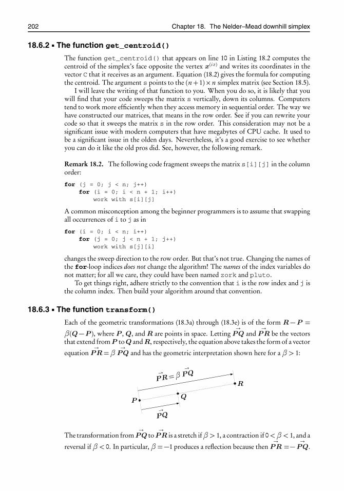
root2014/7/8page 202
�
�
�
�
�
�
�
�
202 Chapter 18. The Nelder–Mead downhill simplex
18.6.2 The function get_centroid()
The function get_centroid() that appears on line 10 in Listing 18.2 computes thecentroid of the simplex’s face opposite the vertex x(i z) and writes its coordinates in thevector C that it receives as an argument. Equation (18.2) gives the formula for computingthe centroid. The argument s points to the (n+1)×n simplex matrix (see Section 18.5).
I will leave the writing of that function to you. When you do so, it is likely that youwill find that your code sweeps the matrix s vertically, down its columns. Computerstend to work more efficiently when they access memory in sequential order. The way wehave constructed our matrices, that means in the row order. See if you can rewrite yourcode so that it sweeps the matrix s in the row order. This consideration may not be asignificant issue with modern computers that have megabytes of CPU cache. It used tobe a significant issue in the olden days. Nevertheless, it’s a good exercise to see whetheryou can do it like the old pros did. See, however, the following remark.
Remark 18.2. The following code fragment sweeps the matrix s[i][j] in the columnorder:
for (j = 0; j < n; j++)for (i = 0; i < n + 1; i++)
work with s[i][j]
A common misconception among the beginner programmers is to assume that swappingall occurrences of i to j as in
for (i = 0; i < n; i++)for (j = 0; j < n + 1; j++)
work with s[j][i]
changes the sweep direction to the row order. But that’s not true. Changing the names ofthe for-loop indices does not change the algorithm! The names of the index variables donot matter; for all we care, they could have been named zork and pluto.
To get things right, adhere strictly to the convention that i is the row index and j isthe column index. Then build your algorithm around that convention.
18.6.3 The function transform()
Each of the geometric transformations (18.3a) through (18.3e) is of the form R−P =
β(Q−P ), where P , Q, and R are points in space. Letting→
PQ and→
PR be the vectorsthat extend fromP toQ andR, respectively, the equation above takes the form of a vector
equation→
PR=β→
PQ and has the geometric interpretation shown here for a β> 1:
P
R
Q
→PQ
→PR=β
→PQ
The transformation from→
PQ to→
PR is a stretch ifβ> 1, a contraction if 0<β< 1, and a
reversal ifβ< 0. In particular, β=−1 produces a reflection because then→
PR =− →PQ.

root2014/7/8page 203
�
�
�
�
�
�
�
�
18.6. The implementation 203
The function transform() that appears on line 12 in Listing 18.2 receives pointsP , Q and a number β and computes R from R−P =β(Q−P ), or equivalently,
R= (1−β)P +βQ. (18.7)
Write an implementation of the function transform(), and add it to your nelder-mead.c.
18.6.4 The function shrink()
The function shrink() that appears on line 14 in Listing 18.2 shrinks the simplextoward the vertex x(ia) according to (18.3e). Actually (18.3e) is a set of n equations,each of which transforms one vertex of the simplex. The obvious way of implementingshrink() is to apply transform() in a loop.
Write an implementation of shrink(), and add it to your nelder-mead.c.
18.6.5 The function replace_row()
Consider the reflection diagram in Figure 18.1. What should the program do when thealgorithm decides to accept x(r ) as the replacement for x(i z)? It will have to replace rowi z of the matrix s with the coordinates of the point x(r ). Here is one possible way ofdoing this:
for (j = 0; j < n; j++)s[iz][j] = r[j];
(Here I have writtenr for the pointer to the array of length n that holds the coordinates ofthe point x(r ).) The same effect may be achieved with much greater efficiency by simplyexchanging the pointers to the vector x(r ) and the matrix’s row i z:
double *tmp = s[iz];s[iz] = r;r = tmp;
This accomplishes the previous version’s for-loop (and n assignments) in exactly threeassignments (independently of n). The savings can be significant if n is large. Since suchexchanges are called for in several places in the algorithm, it makes sense to isolate the ex-change code into a function. That is done in the function replace_row() that appearson line 15 in Listing 18.2. Here is a very wrong implementation of replace_row():
/∗ wrong ! ∗/static inline void replace_row(double **s, int i, double *r){
double *tmp = s[iz];s[iz] = r;r = tmp;
}
That code’s last line gives away what is wrong with it. Assigning a value to r justbefore leaving accomplishes nothing because r is a private variable within the functionreplace_row(); it goes away as soon as the function returns, so any assignment to itis a waste.
The correct way is to set things up so that replace_row() receives not the valueof the pointer r but its address. Then replace_row() will be able to write into that

root2014/7/8page 204
�
�
�
�
�
�
�
�
204 Chapter 18. The Nelder–Mead downhill simplex
Listing 18.3: Here is the correct implementation of the function replace_row(). The argu-ment r is the address of a pointer to a vector (in other words, a pointer to a pointer),and hence the double asterisks.
1 static void inline replace_row(double **s, int i, double **r)2 {3 double *tmp = s[i];4 s[i] = *r;5 *r = tmp;6 }
address, which will retain its value after replace_row() returns. Listing 18.3 showsthe correct implementation.
Be sure to understand what it does, and then add it to your nelder-mead.c.
18.6.6 The function done()
The purpose of the function done() that appears on line 17 in Listing 18.2 is to testwhether the termination conditions in (18.6) have been reached. It returns true if yes andfalse if no. The arguments are the simplex s, the vector y of length n+1 that holds theobjective function’s values evaluated at the vertices, the indices ia and iz of the best andworst vertices, and the argument err2 which has the value (h× tol)2 because that’s whatis needed in (18.6).
Write an implementation of done(), and add it to your nelder-mead.c.
18.6.7 The function nelder_mead()
The prototype of the function nelder_mead() appears on line 19 in Listing 18.2. Itimplements the Nelder–Mead simplex algorithm with the help of the auxiliary functionsalready described.
The function is somewhat long; therefore I have broken it into two pieces. Listing 18.4shows the top part of the function; it deals mainly with housekeeping tasks. It defines thealiases s, n, h, and tol as shorthands for nm→s, etc., because these occur so frequentlyin the code. The variable err2 plays the role of ε2 of (18.6).
The pointers y, C, Pr, Pe, Pc declared on line 8 are going to be set to point to variousvectors. Specifically, y will point to a vector of length n + 1 that will hold the valuesof the objective function at the simplex’s vertices. The pointer C will point to vector oflength n that will hold the coordinates of the centroid x which we encountered in thedescription of the algorithm. The pointers Pr, Pe, Pc will point to vectors of length neach that will hold the coordinates of the points x(r ), x(e), x(c). The variables yr, ye, ycwill hold the values of the objective function evaluated at the points x(r ), x(e), x(c). Thevariable simplex_to_be_freed is a Boolean flag; it is set to false if the user suppliesthe simplex matrix s; otherwise it is set to true. Near the end of nelder_mead(),just before it returns, the memory associated with the simplex matrix will be freed ifsimplex_to_be_freed is true. Otherwise the function’s caller (who supplied thematrix) is responsible for freeing it.
The variable fevalcount keeps a count of the evaluations of the objective function.It is nelder_mead()’s return value.
The last five lines of Listing 18.4 call the macro make_vector() from array.h toallocate memory for the vectors y, C, Pr, Pe, Pc.

root2014/7/8page 205
�
�
�
�
�
�
�
�
18.6. The implementation 205
Listing 18.4: An outline of the function nelder_mead() – part 1.
1 int nelder_mead(struct nelder_mead *nm)2 {3 double **s = nm→s;4 int n = nm→n;5 double h = nm→h;6 double tol = nm→tol;7 double err2 = (h*tol)*(h*tol);8 double *y, *C, *Pr, *Pe, *Pc;9 double yr, ye, yc;
10 int ia, iy, iz;11 int simplex_to_be_freed = 0;12 int fevalcount;13 int i, j;14
15 make_vector(y, n+1); // vertex values16 make_vector(Pr, n); // the reflected point x (r )
17 make_vector(Pe, n); // the expanded point x (e)
18 make_vector(Pc, n); // the contracted ponts x (c)
19 make_vector(C, n); // centroid of the face opposite vertex i z
Let us turn now to the second part of the function nelder_mead(), shown in List-ing 18.5. Normally the user sets the member s of the struct nelder_mead to NULL,which has the effect of delegating the construction of the simplex matrix to the functionnelder_mead(). In that case, the make_matrix() macro from array.h is invokedon line 21 to build that matrix. Then the flag simplex_to_be_freed is set to trueto signal that the memory allocated here should be freed before the function returns.I have left out the part where the entries s[i][j] of the matrix are assigned values. Doit according to (18.5).
Lines 25–27 evaluate the objective function at the simplex’s vertices and store theirvalues in the vector y. Since that takes n + 1 function evaluations, fevalcount is ini-tialized to n+1. Remember to update fevalcount upon every future evaluation of theobjective function.
Let us turn for a moment to the last few lines of Listing 18.5. There we free all the allo-cated memory and return fevalcount, the number of times that the objective functionwas evaluated, to the caller. Note the checking of thesimplex_to_be_freed flag; thisfunction shouldn’t free memory that was handed to it by the caller.
The bulk of Listing 18.5 is one big while-loop, beginning on line 29 and ending online 57. It loops for as long as fevalcount ≤ nm→maxevals. The while-loop’sbody follows closely the algorithmic steps in Section 18.2. Thus, rank_vertices()is called on line 30 to determine the simplex’s best, worst, and next to worst vertices;then done() is called to see whether the termination criteria are met, and if so, theny[ia], which is the value of the objective function at the simplex’s best vertex, is copiedto nm→minval. This is what the caller will see as the sought minimum value. We alsocopy the coordinates of the simplex’s best vertex, that is, row ia of the simplex matrix,into the vector nm→x to let the caller know where the minimum occurred. Line 33 is aplaceholder for that. Do it yourself. The break on line 34 terminates the while-loop.
If the call to done() returns false, control transfers to line 36, where the process of re-flecting, expanding, contracting, and shrinking the simplex begins. Thus, the centroid C

root2014/7/8page 206
�
�
�
�
�
�
�
�
206 Chapter 18. The Nelder–Mead downhill simplex
Listing 18.5: An outline of the function nelder_mead() – part 2.
20 if (s == NULL) { // build simplex if not supplied by user21 make_matrix(s, n+1, n);22 simplex_to_be_freed = 1;23 � assign values to s[i][j]; // see (18.5)24 }25 for (i = 0; i < n + 1; i++)26 y[i] = nm→f(s[i], n, nm→params);27 fevalcount = n+1;28
29 while (fevalcount ≤ nm→maxevals) {30 rank_vertices(y, n+1, &ia, &iy, &iz);31 if (done(s, n, y, ia, iz, err2)) {32 nm→minval = y[ia];33 � copy the best vertex into the vector nm→x ...34 break;35 }36 get_centroid(s, n, iz, C);37 transform(C, s[iz], n, -REFLECT, Pr);38 yr = nm→f(Pr, n, nm→params);39 fevalcount++;40
41 if (yr < y[ia]) { // Case 142 transform(C, Pr, n, EXPAND, Pe);43 ye = nm→f(Pe, n, nm→params);44 fevalcount++;45 if (ye < yr) {46 replace_row(s, iz, &Pe);47 y[iz] = ye;48 } else {49 replace_row(s, iz, &Pr);50 y[iz] = yr;51 }52 } else if (yr < y[iy]) { // Case 253 � ...54 } else { // Cases 3 and 455 � ...56 }57 } // end of the while-loop58
59 � free vectors y, C, Pr, Pe, Pc60 if (simplex_to_be_freed)61 free_matrix(s);62 return fevalcount;63 }
of the face opposite the worst vertex is computed on line 36; then transform() is calledto determine the reflection Pr of the worst vertex through C. Line 38 evaluates the objec-tive function at Pr and assigns it to yr; then fevalcount is incremented. This bringsthe program to where the description of the four cases begins on page 195. On lines 41–51I have implemented Case 1. I have left the remaining three cases to you to complete.

root2014/7/8page 207
�
�
�
�
�
�
�
�
18.7. Project Nelder–Mead: Unconstrained optimization 207
Remark 18.3. Remember that an application of shrink() in Case 3 and Case 4,moves n of the simplex’s n + 1 vertices. Therefore you should update the vector y[]by reevaluating the objective function at the moved vertices and update fevalcountaccordingly.
Remark 18.4. Once you implement the four cases, you will observe that the code forhandling Case 3 is almost identical to that of Case 4. See if you can streamline the logicto eliminate duplicate code.
18.7 Project Nelder–Mead: Unconstrained optimization
Part 18.1. It’s time to give our Nelder–Mead minimizer a try. The file demo-2D.c ofListing 18.6 gives a rather trivial demo of the utility. It is set up to minimize the functionf (x, y) = 3+ (x − 2)2 + (y − 1)2. If all goes well, it will find the minimum value of 3which occurs at the point (2,1), or actually something very close to that, depending on thesetting of the tol value. The demo illustrates the basics of initializing thenelder_meadstructure, calling nelder_mead(), and interpreting the results. See if your code findsthe minimum correctly. Here is what mine does:
$ ./demo-2Dconverged after 87 function evaluationsComputed solution: min = 3 at (1.99999, 1)
Remark 18.5. The initialization of struct nelder_mead in demo-2D.c takes advan-tage of a feature introduced in C99, whereby a structure’s members may be initialized bynaming them. See the discussion under the heading Initializing structures on page 6.
Part 18.2. Here is a more interesting minimization exercise (still in two dimensions).(This is an extremely special case of a truss—a subject treated fully in Chapter 19.) Con-sider a simple two-dimensional structure made of two elastic rods, AC and BC , hinged attheir ends, where A(0,0) and B(1,0) are fixed, but C (1,1) is free to move in the verticalplane when a load is applied to it. The rods elongate and shorten to accommodate theload, but they don’t bend. We wish to determine the structure’s deformed shape when aload vector ⟨a, b ⟩ is applied at C .
A B
C (1,1)
The load-free stateC is at (1,1)
⟨a, b ⟩
A B
C (x, y)
Deformation due to load ⟨a, b ⟩C moves from (1,1) to (x, y)
The mechanics of an elastic rod are completely characterized by its stored energy func-tion W that measures the energy required to stretch or compress a rod of unit length and
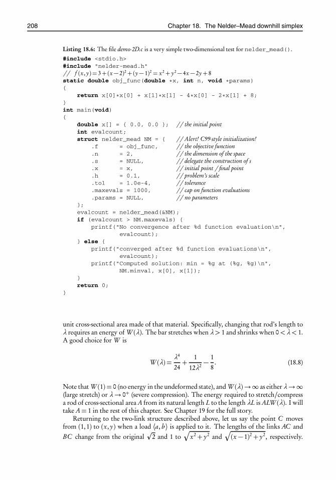
root2014/7/8page 208
�
�
�
�
�
�
�
�
208 Chapter 18. The Nelder–Mead downhill simplex
Listing 18.6: The file demo-2D.c is a very simple two-dimensional test for nelder_mead().
#include <stdio.h>#include "nelder-mead.h"// f (x, y) = 3+ (x− 2)2+ (y− 1)2 = x2+ y2− 4x − 2y+ 8static double obj_func(double *x, int n, void *params){
return x[0]*x[0] + x[1]*x[1] - 4*x[0] - 2*x[1] + 8;}int main(void){
double x[] = { 0.0, 0.0 }; // the initial pointint evalcount;struct nelder_mead NM = { // Alert! C99-style initialization!
.f = obj_func, // the objective function
.n = 2, // the dimension of the space
.s = NULL, // delegate the construction of s
.x = x, // initial point / final point
.h = 0.1, // problem’s scale
.tol = 1.0e-4, // tolerance
.maxevals = 1000, // cap on function evaluations
.params = NULL, // no parameters};evalcount = nelder_mead(&NM);if (evalcount > NM.maxevals) {
printf("No convergence after %d function evaluation\n",evalcount);
} else {printf("converged after %d function evaluations\n",
evalcount);printf("Computed solution: min = %g at (%g, %g)\n",
NM.minval, x[0], x[1]);}return 0;
}
unit cross-sectional area made of that material. Specifically, changing that rod’s length toλ requires an energy of W (λ). The bar stretches when λ> 1 and shrinks when 0<λ< 1.A good choice for W is
W (λ) =λ4
24+
1
12λ2 −1
8. (18.8)
Note that W (1) = 0 (no energy in the undeformed state), and W (λ)→∞ as either λ→∞(large stretch) or λ→ 0+ (severe compression). The energy required to stretch/compressa rod of cross-sectional area A from its natural length L to the length λL is ALW (λ). I willtake A= 1 in the rest of this chapter. See Chapter 19 for the full story.
Returning to the two-link structure described above, let us say the point C movesfrom (1,1) to (x, y) when a load ⟨a, b ⟩ is applied to it. The lengths of the links AC and
BC change from the original�
2 and 1 to�
x2+ y2 and�(x − 1)2+ y2, respectively.

root2014/7/8page 209
�
�
�
�
�
�
�
�
18.7. Project Nelder–Mead: Unconstrained optimization 209
It follows that structure’s total energy is
� (x, y) =�
2W��
x2+ y2
�2
�+W
*�(x − 1)2+ y2
+− a(x − 1)− b (y − 1). (18.9)
The last two terms express the work due to the displacement of the load.It is shown in Chapter 19 that the structure’s equilibria (in general there are multiple
equilibrium states) correspond to the stationary points of the energy function � (x, y).68
If the stationary point is a (local or global) minimum, the equilibrium is stable. If thestationary point is a (local or global) maximum or a saddle, the equilibrium is unstable.
Figure 18.2 shows the graphs and level sets of the energy function � (x, y) in two casestudies. In Case study 1 the load is ⟨0,−0.3⟩. The energy function has three stationarypoints: D1 is the global minimum; D2 and D3 are saddles. In Case study 2 the load is⟨0,−0.1⟩. The energy function has five stationary points: D1 and D2 are minima; D3, D4,and D5 are saddles. The drawings along the bottom of Figure 18.2 show the structure’sthree possible equilibrium configurations corresponding to Case study 1. Can you drawthe five equilibrium configurations for Case study 2? You need not do any calculationsfor this; just examine the energy surface and the positions of the five equilibria.
The Nelder–Mead algorithm is ideally suited for finding the local minima of � (x, y).69
Write a program demo-energy.c to compute the coordinates of the equilibrium point D1in Case study 1 and the equilibrium points D1 and D2 in Case study 2. In Case study 1my program prints
$ ./demo-energyExpected answer: min = -0.6395281605 at (0.8319642234, -1.2505278260)Computed solution: min = -0.6395281277 at (0.8315845906, -1.2505201990)Converged after 71 function evaluations
The solution given on the “Expected answer” line is correct in all its digits. I computed thatindependently by solving the system of nonlinear equations
,∂ �/∂ x = 0,∂ �/∂ y = 0
-with high precision in Maple and then pasted the answer into demo-energy.c for compar-ison with the Nelder–Mead result. As to the computation’s parameters, I took h=1.0,tol=1.0e-3 and chose (−1,1) for the starting point just to be nasty since that’s so ob-viously far from the expected equilibrium. I initialized the simplex to NULL to let theprogram build the simplex on its own.
To help you check your results, here are the coordinates and function values of thelocal minima D1 and D2 of Case study 2:
D1: min = -0.2047379473 at (0.9208762303, -1.0926128103)D2: min = -0.0055676481 at (1.1554672673, 0.8776603419)
Remark 18.6. The load ⟨a, b ⟩ enters the energy function (18.9) as a parameter. See ifyou can set up your code so that the energy function reads the load vector through itsparams argument.
Remark 18.7. The “smokestacks” in the graphs in Figure 18.2 are inherited from thevertical asymptote at zero of the function W (x) in (18.8). They tell us that � (x, y)→+∞as the point C is pushed too close to the points A or B . (Do you see that?) In particular,� is undefined at A and B . This raises a serious concern: what would happen if a vertex
68A stationary point (also called a critical point) of a function f (x) : Rn →R is where∇ f (x) = 0.69Nelder–Mead cannot find saddle points. I found the coordinates of the saddle points D2 and D3 shown in
Figure 18.2 by solving directly the nonlinear system of equations ∂ �/∂ x = 0 and ∂ �/∂ y = 0.

root2014/7/8page 210
�
�
�
�
�
�
�
�
210 Chapter 18. The Nelder–Mead downhill simplex
Case study 1: load = ⟨0,−0.3⟩.D1
D2
D3A
B
Case study 2: load = ⟨0,−0.1⟩.
D1
D2
D3
D4
D5A
B
load
A B
C
D1
load
A B
C
D2
loadA B
C
D3
A(0,0) B(1,0) C (1,1)
D1(0.83,−1.25) D2(0.59,0.03) D3(−0.67,0.42)
Figure 18.2: The plots at the top are the graphs and level sets of the energy func-tion (18.9) corresponding to (a) Case study 1 (on the left) where the loadis ⟨a, b ⟩ = ⟨0,−0.3⟩, and (b) Case study 2 (on the right) where the load is⟨a, b ⟩= ⟨0,−0.1⟩. The former has three stationary points: D1 is the globalminimum; D2 and D3 are saddles. The latter has five stationary points: D1and D2 are minima; D3, D4, and D5 are saddles. I have shown the plots ofthe energy surface from two different perspectives in order to convey a bet-ter sense of what they look like. The drawings along the bottom show thetruss’s three possible configurations corresponding to Case study 1. Youdo similar drawings for Case study 2.
of the simplex steps on either A or B during the iteration? The outcome of that eventdepends on your compiler. It may be set up to handle a floating point division by zerogracefully and produce an “infinity” which is larger than all possible floating numbers,or it may just crash the program. To be on the safe side, it would be a good idea to chop

root2014/7/8page 211
�
�
�
�
�
�
�
�
18.8. Constrained optimization 211
off and flatten the smokestacks at a sufficiently large elevation to avoid them running toinfinity. That certainly will not affect the locations of W ’s minima, which are the objectsof our interest. Thus, noting that W (10−3)≈ 83333, it would be safe to redefine W as
1 double W(double x)2 {3 double eps = 1.0e-3;4 if (x < eps)5 x = eps;6 W(x) = ... � // enter (18.8) here7 }
Part 18.3. Try your Nelder–Mead on a function of one variable. Write a programdemo-1D.c to minimize the function
f (x) = x2− 2x + 2= (x − 1)2+ 1.
18.8 Constrained optimizationThe simplex algorithm may be applied to minimization problems subject to constraintsof certain types, as Nelder and Mead point out in their article [49]. Affine constraints areparticularly easy to handle. Specifically, let f : Rn →R as before, and let� be an affinespace in Rn defined by
� = {x ∈Rn : Ax= b},where A is an m× n matrix and b is an m-vector. We wish to compute
minx∈� f (x). (18.10)
We assume, without loss of generality, that rank(A) = m because otherwise we may re-duce the matrix to the row echelon form, discard the zero rows that appear at the bottom,and redefine A to what remains, without changing the space � . We also assume m < nbecause otherwise� reduces to a point or an empty set. With such an A, the constraintAx= b is equivalent to a set of m scalar and linearly independent constraints:
n∑j=1
ai j x j = bi , i = 1, . . . , m.
The key to extending the Nelder–Mead algorithm to the constrained problem (18.10)is the realization that the Nelder–Mead transformations, given in (18.3a) through (18.3e)and summarized in (18.7), are affine-preserving in the sense that if the points P and Q arein an affine space� , then the point R= (1−β)P +βQ is also in� . Thus, to solve theproblem (18.10) it suffices to pick the initial simplex within � . Then the transformedsimplexes will remain within� , and if the iteration arrives at a minimizer, it would be asolution of the constrained optimization problem (18.10).
One way to get the initial simplex to lie within� is to pick an unconstrained initialsimplex inRn and project it onto� . It can be shown (see Section 18.10) that the operatorP of the orthogonal projection onto� is given by
Px=�I −AT (AAT )−1A
�x+AT (AAT )−1b, x ∈Rn , (18.11)
where I is the n× n identity matrix and the superscript T denotes the transpose.

root2014/7/8page 212
�
�
�
�
�
�
�
�
212 Chapter 18. The Nelder–Mead downhill simplex
Remark 18.8. If A is a 1×n matrix (that is, it is a row vector,) then the projection operatortakes on a particularly simple form. For convenience, let us introduce the n-vector a =AT . Then the definition of the affine space � takes the form� = {x ∈Rn : a ·x= c},where c is a constant.70 It’s not difficult to verify that the projection formula (18.11)collapses to
Px=x+1
‖a‖2
�c −a ·x a. (18.12)
Remark 18.9. A full-fledged application of either of the projection formulas (18.11)or (18.12) is an overkill in those simple cases where the nature of the projection is evi-dent a priori. For instance, if� is a hyperplane perpendicular to one of the coordinatesaxes, as in
� = ,x= (x1, x2, . . . , x7) ∈R7 : x5 = 12-, (� is perpendicular to the x5 axis),
then projecting the simplex onto� amounts to setting all entries in column 5 of the initialsimplex matrix to 12. Since the transformation (18.7) applied to the simplex matrix leavesa column of constants invariant, the simplex remains in� as it evolves.71 This is how weenforce the immobility of a truss’s fixed joints in Chapter 19.
Remark 18.10. Although projecting a simplex onto a proper affine space flattens it intoa degenerate simplex of zero volume, this does not seem to have an adverse effect on theNelder–Mead algorithm’s operation.
Remark 18.11. It is possible to transform the constrained optimization problem (18.10)to an unconstrained one through elimination of variables. Specifically, we may solve them× n linear system Ax= b for m of the unknowns in terms of the rest. (Recall that weare assuming that rank(A) = m, and m < n.) We eliminate the solved variables in f (x)and thus arrive at an unconstrained function g : Rn−m →R. Applying the Nelder–Meadsimplex algorithm to the unconstrained and lower-dimensional function g is more effi-cient compared to the projection method above—it requires fewer function evaluations,as experiments show. This has to be balanced against the programmer’s time and effortin reducing f to g .
18.9 Project Nelder–Mead: Constrained optimization
Part 18.4. Minimize f (x, y, z) = x2 + y2 + z2 subject to the constraint x + y + z = 3.It is easy to see that the minimum is 3 and occurs at (1,1,1). Write a program, demo-constrained.c, to do that with the projection method. My program says
$ ./demo-constrainedconverged after 140 function evaluationsmin = 3 at (1, 1, 1)
For the parameters I took h=0.1, tol=1.0e-5 and the initial point at (1,2,3). My pro-gram builds the initial simplex according to (18.5) and then projects it onto the constraintspace by applying (18.12).
70Thus,� is a hyperplane in Rn , with a as a normal vector.71This is pointed out in Nelder and Mead’s article [49].

root2014/7/8page 213
�
�
�
�
�
�
�
�
18.10. Appendix: Orthogonal projection onto Ax= b 213
0
Px−v = PN (A)(x−v)
x−v
v
Px
x
N (A)
� = v+N (A)
Figure 18.3: An imitation of a drawing on page 437 of [46].
18.10 Appendix: Orthogonal projection onto Ax = b
Although the projection formula (18.11) is well known among the specialists in linearalgebra, it is difficult to locate in ordinary textbooks. It may be derived through an ap-plication of the singular value decomposition theorem, although that’s an overkill sinceno singular values appear in the formula. Plesník [52] states the formula and refers thereader to Meyer’s book [46]. I did not find an explicit form of the formula there, but thebook offers all the ingredients needed for deriving it. Let me state the result formally as atheorem and then sketch a proof.
Theorem 18.1. Consider the m× n matrix A and the m-vector b, and let
� = {x ∈Rn : Ax= b}.Suppose rank(A) =m. Then the orthogonal projector P : Rn →� is given by
Px=�I −AT (AAT )−1A
�x+AT (AAT )−1b, x ∈Rn ,
where I is the n× n identity matrix.
Proof. The affine space � is parallel to the nullspace N (A) of A since for any u and v in� we have Au= b and Av = b; therefore A(u−v) = 0. Figure 18.3 depicts the origin 0,the nullspace N (A) of A, and the affine space� , which is parallel to N (A). Pick and fix av ∈� , that is, Av = b. It should be clear that� = v+N (A).
The diagram also shows an arbitrary point x ∈ Rn and its orthogonal projectionPx onto � . Subtracting v from both x and Px moves them to x− v and Px− v, asshown, and thus the problem of projecting onto an affine space reduces to the problemof projecting onto a subspace. Writing PN (A) for the orthogonal projector onto N (A), wehave Px−v = PN (A)(x−v). Thus,
Px= v+ PN (A)(x−v).
It remains to characterize the projector PN (A). It can be shown (see page 434 of [46]) thatif A is m × n and rank(A) = n, then PN (AT ) = I −A(AT A)−1AT . It follows that if A is

root2014/7/8page 214
�
�
�
�
�
�
�
�
214 Chapter 18. The Nelder–Mead downhill simplex
m× n and rank(A) =m, then PN (A) = I −AT (AAT )−1A. We conclude that
Px= v+�I −AT (AAT )−1A
�(x−v)
= v+�I −AT (AAT )−1A
�x− �I −AT (AAT )−1A
�v
=�I −AT (AAT )−1A
�x+AT (AAT )−1Av
=�I −AT (AAT )−1A
�x+AT (AAT )−1b.

root2014/7/8page 215
�
�
�
�
�
�
�
�
Chapter 19
Trusses
Prerequisites: Chapters 7, 8, 9, 16, 18
19.1 IntroductionA truss consists of a two- or three-dimensional network of slender links joined at nodes.72
The junctions at the nodes are assumed to be hinge-like; that is, no bending moment istransmitted through a node. External loads are applied only at the nodes. The links arestraight and do not bend.
A truss deforms under loads: links shrink and stretch, nodes move, internal and ex-ternal reaction forces are developed, and the truss either finds a new equilibrium stateor collapses. The natural (unloaded) geometry of a truss is called its reference configura-tion. The shape of a truss after it reaches equilibrium under a set of applied loads is calleddeformed configuration.
Trusses are ubiquitous in our daily lives. We see them in radio and cellular telephonetransmission towers, electric power transmission lines, bridges, roof supports, construc-tion crane booms, and orbital space station platforms, both in fiction and reality.
Figure 19.1 shows a very simple two-dimensional truss supported on two nodes. Theleft node is fully anchored; it cannot move, but the truss can pivot about it. The rightnode is on rollers; it is free to move horizontally but not vertically. Truss bridges aresupported this way. Figure 19.2 is a photograph of a real truss bridge.
A major phase in the structural design and analysis of a truss is the determination ofstresses and strains in its links induced by the externally applied loads. A well-designedtruss utilizes its structural components in an optimal way; it is strong, lightweight, andeconomical. At the same time it should not deform excessively or break under the loadsthat it’s meant to support.
In the traditional engineering practice, the geometry of a truss, i.e., the positions ofits nodes and the links that connect them, is decided in advance. Then cross-sectionalsizes and materials of the links are selected to enable the truss to sustain the anticipatedloads. The geometric design is based on the engineer’s intuition, his/her aesthetic consid-erations, the available structural materials, and his/her experience with robust structuresthat have withstood the test of time.73
72Links and nodes are also known as members and joints, respectively.73Recent developments in the area of topology design of structures replace this ad hoc design process with sophis-
ticated techniques that produce optimally designed structures without a priori assumptions on the geometry.See [8, 3] for more information.
215
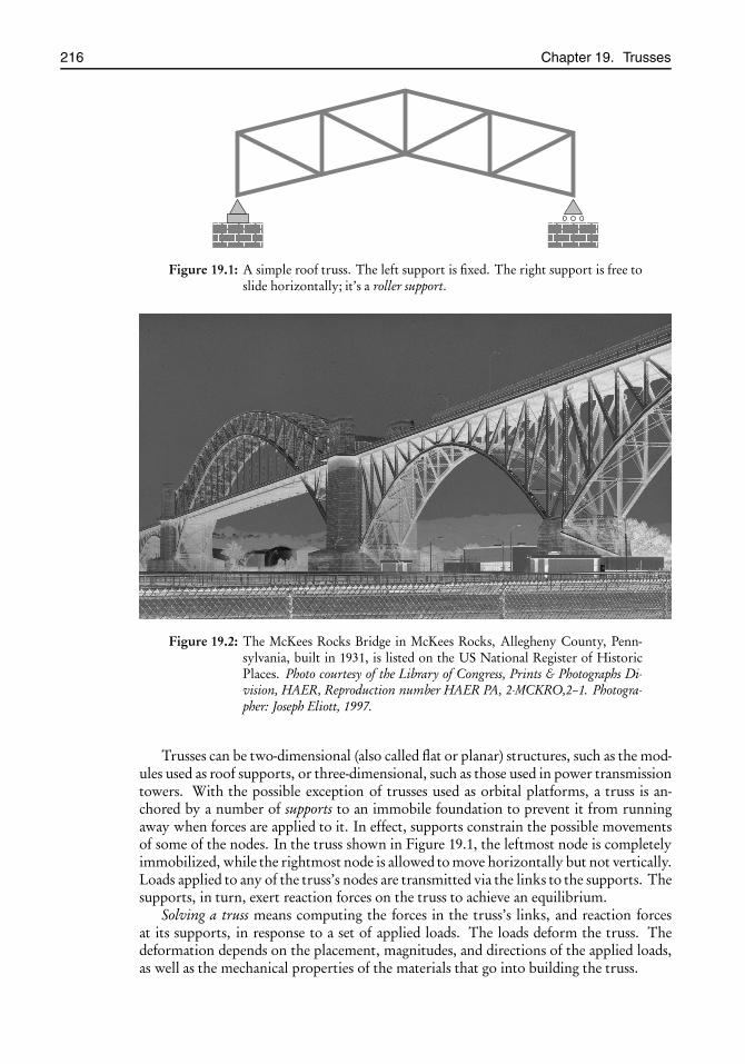
root2014/7/8page 216
�
�
�
�
�
�
�
�
216 Chapter 19. Trusses
Figure 19.1: A simple roof truss. The left support is fixed. The right support is free toslide horizontally; it’s a roller support.
Figure 19.2: The McKees Rocks Bridge in McKees Rocks, Allegheny County, Penn-sylvania, built in 1931, is listed on the US National Register of HistoricPlaces. Photo courtesy of the Library of Congress, Prints & Photographs Di-vision, HAER, Reproduction number HAER PA, 2-MCKRO,2–1. Photogra-pher: Joseph Eliott, 1997.
Trusses can be two-dimensional (also called flat or planar) structures, such as the mod-ules used as roof supports, or three-dimensional, such as those used in power transmissiontowers. With the possible exception of trusses used as orbital platforms, a truss is an-chored by a number of supports to an immobile foundation to prevent it from runningaway when forces are applied to it. In effect, supports constrain the possible movementsof some of the nodes. In the truss shown in Figure 19.1, the leftmost node is completelyimmobilized, while the rightmost node is allowed to move horizontally but not vertically.Loads applied to any of the truss’s nodes are transmitted via the links to the supports. Thesupports, in turn, exert reaction forces on the truss to achieve an equilibrium.
Solving a truss means computing the forces in the truss’s links, and reaction forcesat its supports, in response to a set of applied loads. The loads deform the truss. Thedeformation depends on the placement, magnitudes, and directions of the applied loads,as well as the mechanical properties of the materials that go into building the truss.
root2014/7/8page 217
�
�
�
�
�
�
�
�
19.2. One-dimensional elasticity 217
In structural mechanics, large deformations of structures such as bridges or booms ofa crane are unacceptable. Such structures are designed purposely to deform only imper-ceptibly under loads within the design range; you wouldn’t want to feel a bridge moveunderneath you as you drive over it. A consequence of the small deformation require-ment is that for design purposes the shape of the bridge my be assumed to be independentof the applied forces. The effects of the infinitesimal extensions of the links have onlysecond order effects on the shape and may be ignored in engineering practice. Solvingsuch a truss reduces to solving a system of linear equations.
If, however, we admit large deformations whereby the geometry changes consider-ably under the applied loads, the equilibrium equations form a fully nonlinear system.Nonlinearity enters in the analysis of large deformations from two different sources:(i) geometric nonlinearities are introduced due to the finite deformation of the truss’sgeometry, and (ii) mechanical nonlinearities are introduced because the elastic responseof materials under large deformation is generally nonlinear.
The program developed in this chapter solves trusses that may undergo arbitrarilylarge deformations. Admittedly, large deformations are of no great practical interest;however, they make for an interesting and fun academic exercise. I should emphasize,however, that this does not mean that the program developed here is worthless. Let’snote that if the truss members are sufficiently stiff and the applied loads are not too large,then the truss’s deformation will be small; therefore our solver will pick up the usualsolution of an infinitesimally deformed truss.
Finally, let me point out that I have limited this chapter’s programs to planar trussesonly to simplify the exposition. The theory, however, is developed in the generaln-dimensional context. Extending the programs to three-dimensional trusses is straight-forward and poses no conceptual or programming challenges.
19.2 One-dimensional elasticityAn elastic solid is a material that deforms when you exert forces on it and returns to itsoriginal shape when you remove those forces. At least that’s the intuitive idea. A rubberband, an automobile tire, a baseball, and a coiled spring are good examples of elastic solids.Less conspicuous elastic behavior is all around us. You sit on a seat cushion and it deformsto accommodate you; you rise and it bounces back to its original shape. A skyscrapersways in high winds and earthquakes. When the wind and seisms subside, it returns toits upright position. A bridge sags when a train passes over it. It resumes its normalshape when the train is gone. A paper clip is elastic in small deformations; it regains itsoriginal shape when you remove it from a thin stack of papers. It is not elastic under largedeformations; if you bend it severely, it will not return to its original shape. What we havethere is plastic behavior. That is the subject of study in the theoretical and experimentalplasticity. We won’t deal with plasticity in this book.
Theoretical elasticity is a deep and interesting subject. In this section I will present avery special case of elasticity as it applies to one-dimensional deformations, that is, defor-mations that are dominated by displacements in a single direction. The stretching of arubber band is an example of one-dimensional deformations, but the deformation of anautomobile tire where it hits the ground is not.
19.2.1 Stress
Figure 19.3 shows an elastic solid specimen in the shape of a cylinder of length L andcross-sectional area A in its natural (undeformed) state. It also shows the deformed shape
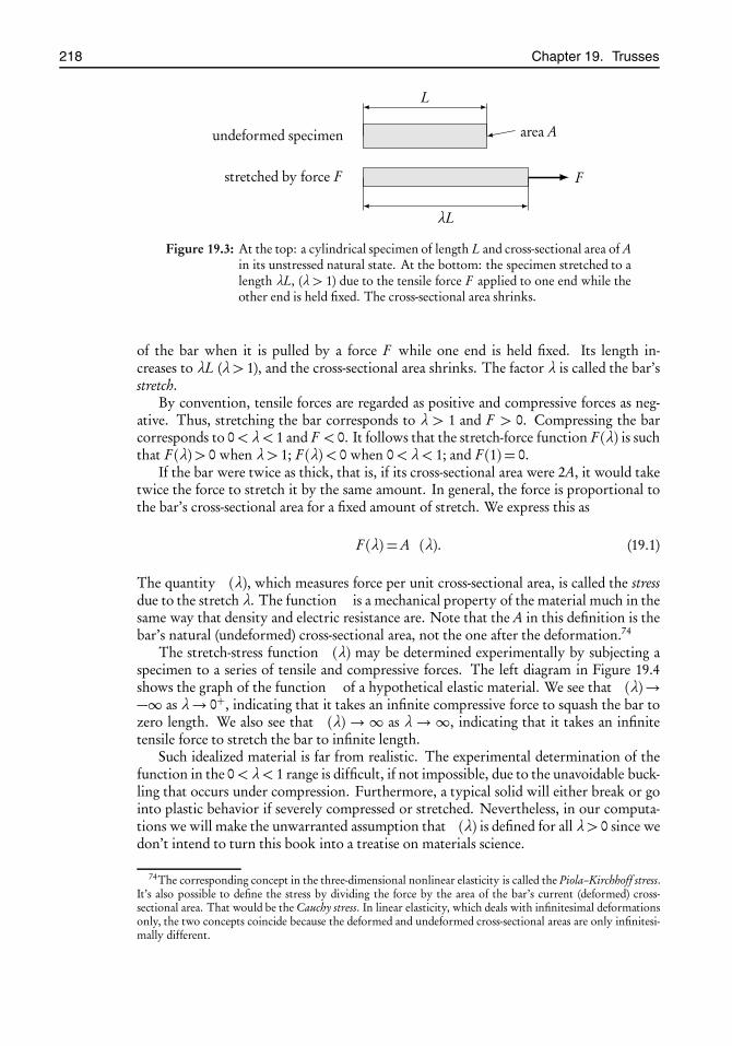
root2014/7/8page 218
�
�
�
�
�
�
�
�
218 Chapter 19. Trusses
undeformed specimen
L
area A
Fstretched by force F
λL
Figure 19.3: At the top: a cylindrical specimen of length L and cross-sectional area of Ain its unstressed natural state. At the bottom: the specimen stretched to alength λL, (λ > 1) due to the tensile force F applied to one end while theother end is held fixed. The cross-sectional area shrinks.
of the bar when it is pulled by a force F while one end is held fixed. Its length in-creases to λL (λ > 1), and the cross-sectional area shrinks. The factor λ is called the bar’sstretch.
By convention, tensile forces are regarded as positive and compressive forces as neg-ative. Thus, stretching the bar corresponds to λ > 1 and F > 0. Compressing the barcorresponds to 0< λ< 1 and F < 0. It follows that the stretch-force function F (λ) is suchthat F (λ)> 0 when λ > 1; F (λ)< 0 when 0< λ< 1; and F (1) = 0.
If the bar were twice as thick, that is, if its cross-sectional area were 2A, it would taketwice the force to stretch it by the same amount. In general, the force is proportional tothe bar’s cross-sectional area for a fixed amount of stretch. We express this as
F (λ) =Aσ(λ). (19.1)
The quantity σ(λ), which measures force per unit cross-sectional area, is called the stressdue to the stretch λ. The function σ is a mechanical property of the material much in thesame way that density and electric resistance are. Note that the A in this definition is thebar’s natural (undeformed) cross-sectional area, not the one after the deformation.74
The stretch-stress function σ(λ) may be determined experimentally by subjecting aspecimen to a series of tensile and compressive forces. The left diagram in Figure 19.4shows the graph of the function σ of a hypothetical elastic material. We see that σ(λ)→−∞ as λ→ 0+, indicating that it takes an infinite compressive force to squash the bar tozero length. We also see that σ(λ) → ∞ as λ → ∞, indicating that it takes an infinitetensile force to stretch the bar to infinite length.
Such idealized material is far from realistic. The experimental determination of thefunction in the 0< λ< 1 range is difficult, if not impossible, due to the unavoidable buck-ling that occurs under compression. Furthermore, a typical solid will either break or gointo plastic behavior if severely compressed or stretched. Nevertheless, in our computa-tions we will make the unwarranted assumption that σ(λ) is defined for all λ> 0 since wedon’t intend to turn this book into a treatise on materials science.
74The corresponding concept in the three-dimensional nonlinear elasticity is called the Piola–Kirchhoff stress.It’s also possible to define the stress by dividing the force by the area of the bar’s current (deformed) cross-sectional area. That would be the Cauchy stress. In linear elasticity, which deals with infinitesimal deformationsonly, the two concepts coincide because the deformed and undeformed cross-sectional areas are only infinitesi-mally different.
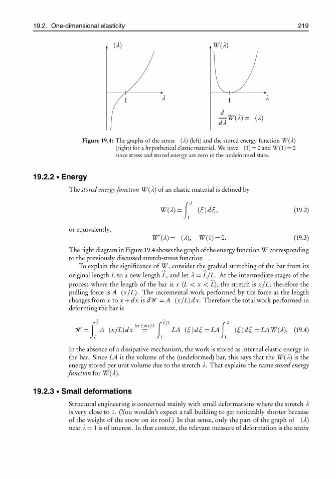
root2014/7/8page 219
�
�
�
�
�
�
�
�
19.2. One-dimensional elasticity 219
λ
σ(λ)
1 λ
W (λ)
1
d
dλW (λ) = σ(λ)
Figure 19.4: The graphs of the stress σ (λ) (left) and the stored energy function W (λ)(right) for a hypothetical elastic material. We have σ (1) = 0 and W (1) = 0since stress and stored energy are zero in the undeformed state.
19.2.2 Energy
The stored energy function W (λ) of an elastic material is defined by
W (λ) =∫ λ
1σ(ξ )dξ , (19.2)
or equivalently,W ′(λ) = σ(λ), W (1) = 0. (19.3)
The right diagram in Figure 19.4 shows the graph of the energy function W correspondingto the previously discussed stretch-stress function σ .
To explain the significance of W , consider the gradual stretching of the bar from itsoriginal length L to a new length .L, and let λ = .L/L. At the intermediate stages of theprocess where the length of the bar is x (L < x < .L), the stretch is x/L; therefore thepulling force is Aσ(x/L). The incremental work performed by the force as the lengthchanges from x to x + d x is d� = Aσ(x/L)d x. Therefore the total work performed indeforming the bar is
� =∫ .L
LAσ(x/L)d x
let ξ=x/L=
∫ .L/L
1LAσ(ξ )dξ = LA
∫ λ
1σ(ξ )dξ = LAW (λ). (19.4)
In the absence of a dissipative mechanism, the work is stored as internal elastic energy inthe bar. Since LA is the volume of the (undeformed) bar, this says that the W (λ) is theenergy stored per unit volume due to the stretch λ. That explains the name stored energyfunction for W (λ).
19.2.3 Small deformations
Structural engineering is concerned mainly with small deformations where the stretch λis very close to 1. (You wouldn’t expect a tall building to get noticeably shorter becauseof the weight of the snow on its roof.) In that sense, only the part of the graph of σ(λ)near λ= 1 is of interest. In that context, the relevant measure of deformation is the strain
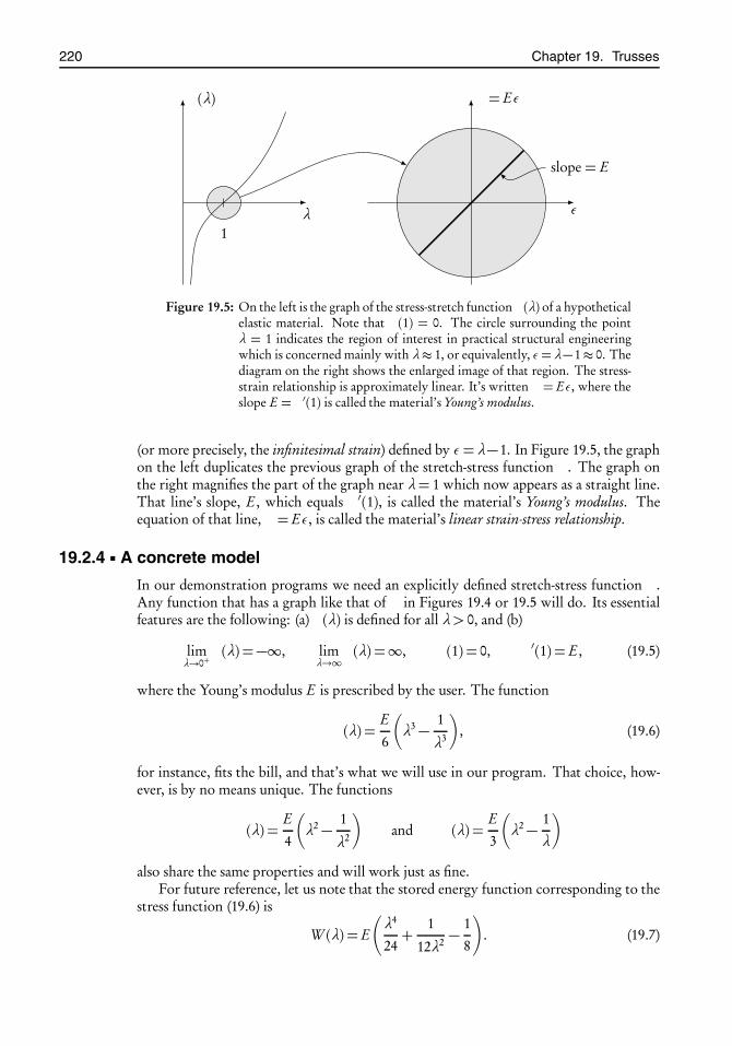
root2014/7/8page 220
�
�
�
�
�
�
�
�
220 Chapter 19. Trusses
λ
σ(λ)
1
ε
σ = Eε
slope = E
Figure 19.5: On the left is the graph of the stress-stretch function σ (λ) of a hypotheticalelastic material. Note that σ (1) = 0. The circle surrounding the pointλ = 1 indicates the region of interest in practical structural engineeringwhich is concerned mainly with λ≈ 1, or equivalently, ε= λ−1≈ 0. Thediagram on the right shows the enlarged image of that region. The stress-strain relationship is approximately linear. It’s written σ = Eε, where theslope E = σ ′(1) is called the material’s Young’s modulus.
(or more precisely, the infinitesimal strain) defined by ε= λ−1. In Figure 19.5, the graphon the left duplicates the previous graph of the stretch-stress function σ . The graph onthe right magnifies the part of the graph near λ= 1 which now appears as a straight line.That line’s slope, E , which equals σ ′(1), is called the material’s Young’s modulus. Theequation of that line, σ = Eε, is called the material’s linear strain-stress relationship.
19.2.4 A concrete model
In our demonstration programs we need an explicitly defined stretch-stress function σ .Any function that has a graph like that of σ in Figures 19.4 or 19.5 will do. Its essentialfeatures are the following: (a) σ(λ) is defined for all λ > 0, and (b)
limλ→0+
σ(λ) =−∞, limλ→∞σ(λ) =∞, σ(1) = 0, σ ′(1) = E , (19.5)
where the Young’s modulus E is prescribed by the user. The function
σ(λ) =E
6
�λ3− 1
λ3
�, (19.6)
for instance, fits the bill, and that’s what we will use in our program. That choice, how-ever, is by no means unique. The functions
σ(λ) =E4
�λ2− 1
λ2
�and σ(λ) =
E3
�λ2− 1
λ
�also share the same properties and will work just as fine.
For future reference, let us note that the stored energy function corresponding to thestress function (19.6) is
W (λ) = E
!λ4
24+
1
12λ2 −1
8
$. (19.7)

root2014/7/8page 221
�
�
�
�
�
�
�
�
19.3. From energy to force 221
19.3 From energy to forceConsider a rod of natural length L and cross-sectional area A, one end of which is attachedto, and can pivot about, a fixed point in space, call it a, and the other end is free to bepushed, pulled, and moved about; call it x.
f
a
x
‖x−a‖fixed
pivot
Let f be the force vector applied at x, and let e(x) be the elastic energy stored in therod. I will show that the gradient of e(x) equals f . Stated in symbols,
∇e(x) = f . (19.8)
To see why, note that the rod’s length is ‖x−a‖; therefore, according to (19.4), its elasticenergy is
e(x) = LAW�‖x−a‖
L
�.
Compute the gradient by applying the chain rule from multivariable calculus. We get
∇e(x) = LAW ′�‖x−a‖
L
�1
L
x−a
‖x−a‖ .
Now, (‖x−a‖)/L is the bar’s stretch, λ, and W ′(λ) = σ(λ) according to (19.3), so we get
∇e(x) =Aσ(λ)x−a
‖x−a‖ .
According to (19.1), Aσ(λ) is the magnitude of the applied force. Since the expression(x−a)/‖x− a‖ is a unit vector along the bar’s direction, the product of the two is theapplied force vector, as asserted.
Remark 19.1. Here I want to change the notation on you and rewrite (19.8) as
ddx
e(x) = f . (19.8’)
The change may look odd at first sight, but it’s perfectly legal as long as one defines whatis meant by the notation d/dx, where x is not a scalar. But that’s nothing new. Considera function f : X → Y , where X and Y are normed spaces (they need not be finite dimen-sional even). The Fréchet derivative D f of f at a point x ∈X is a bounded linear operator(D f )(x) : X →Y such that
limh→0
/// f (x + h)− f (x)− �(D f )(x)�(h)
///Y
‖h‖X= 0.

root2014/7/8page 222
�
�
�
�
�
�
�
�
222 Chapter 19. Trusses
0 5 10
14
1383
1
7
11
2
6
124 9
0 1 2 3
4 5 6 7
F 3
F 7
Figure 19.6: On the left we see a cantilever truss of eight nodes and 15 links in its nat-ural (unloaded) state. Nodes and links are numbered independently, in noparticular order. Nodes 0 and 4 are anchored and immobile; all others aremovable. On the right we see the deformed truss under the loads appliedat nodes 3 and 7.
When X = R and Y = R, this agrees with the definition of the derivative in freshmancalculus. If X =Rn and Y =R, this agrees with the definition of the gradient in multi-variable calculus. In (19.8’) I have taken the liberty of changing the notation (De)(x) to
ddx e(x), as it is more expressive for our purposes.
19.4 The energy of a trussThe left drawing in Figure 19.6 depicts a two-dimensional cantilever truss consisting ofeight nodes (labeled 0–7) and 15 links (labeled 0–14). Nodes 0 and 4 are anchored to awall and cannot move. The other nodes are free to move in response to applied loads.The right drawing in Figure 19.6 shows the truss’s deformed state under loads applied tonodes 3 and 7. In general, loads may be applied to any of the nodes.
Generalizing from that concrete example, let us consider a two- or three-dimensionaltruss of n nodes, labeled 0,1, . . . , n−1, and l links, labeled 0,1, . . . , l −1. The order of theenumeration of the nodes and links is immaterial.
For each link p, where p ∈ {0,1, . . . , l − 1}, let Lp and Ap denote the link’s unde-formed length and cross-sectional area, Wp be the stored energy function of the link’smaterial, and λp be the link’s stretch after the truss is loaded.
Furthermore, for each node q , where q ∈ {0,1, . . . , n− 1}, let F q denote the externalload (a vector) applied to the node q , and let �xq and xq be the node’s position in spacebefore and after loading, respectively.
Any arbitrary choice of positions {x0,x1, . . . ,xn−1} of the n nodes defines a (gener-ally nonequilibrium) configuration of the truss in space. We define the total energy �associated with that configuration as
� (x0,x1, . . . ,xn−1) =l−1∑p=0
Ap LpWp(λp)−n−1∑q=0
F q · (xq −�xq ). (19.9)
The first summation expresses the total elastic energy stored in the links in that config-uration. The second summation is the total work done by the loads due to their dis-placements. Let us observe that since the positions of a truss’s nodes determines the(deformed) lengths of the truss’s links, the stretches λp are easily computed in terms of{x0,x1, . . . ,xn−1}.

root2014/7/8page 223
�
�
�
�
�
�
�
�
19.5. From energy to equilibrium 223
F k
F k
xk
xk + dxk
Figure 19.7: This shows a fragment of a truss, with a focus on the node xk and fourlinks that radiate from it. An external load F k is acting on the node. Tointerpret the partial derivative ∂ �/∂ xk , displace the node xk by a smallamount dxk while keeping all other nodes fixed. We show that the changein energy in that deformation equals the sum of the internal and externalforces applied to xk .
We will see the significance of the definition (19.9) when we analyze its implicationsin the next section.
19.5 From energy to equilibriumConsider the truss of n nodes and l links introduced in the previous section. Figure 19.7shows a fragment of that truss, with a focus on some node xk which has four links radi-ating from it. The choice of four links is for illustration only; the argument that followsis independent of the number of links that join at xk . The nodes at the other ends of thelinks are shown as little circles, but their labels are not since those labels are irrelevant tothe argument that follows.
The truss’s total energy � (x0,x1, . . . ,xn−1) is defined in (19.9). We may calculate thepartial derivatives of � with respect to each of its arguments with the help of the dif-ferentiation formula (19.8’). But before we do that, let us examine the meaning of thatoperation. The differential
�∂ �/∂ xk
·dxk measures the change in � as the node xk isdisplaced to a location xk +dxk while all other nodes are held fixed. Figure 19.7 shows the“before” and “after” geometries.
Since all nodes except xk are held fixed, the only links that change in length are thosethat connect to xk . Therefore the summation over p in (19.9) reduces to a sum over thoselinks that connect to xk . Similarly, the summation over q reduces to a single term sincenodes other than xk do not move. In summary,
∂ �∂ xk
·dxk =0 ∑
p∈ links to xk
∂
∂ xk
�Ap LpWp(λp)
−F k1·dxk .
According to the differentiation formula (19.8’), each term in the summation above equalsthe force vector f p within the corresponding link. Therefore the equation above takesthe form
∂ �∂ xk
·dxk =0* ∑
p∈ links to xk
f p+−F k
1·dxk .

root2014/7/8page 224
�
�
�
�
�
�
�
�
224 Chapter 19. Trusses
This is an extremely important result! The quantity in the square brackets is the vectorsum of all forces (internal and external) applied to the point xk . When the truss is inequilibrium, the sum of the forces applied to xk should be zero (this is Newton’s second law;otherwise xk must accelerate). We conclude that the left-hand side is zero. But since dxk
is arbitrary, then the derivative of � is zero. We state this as the following.
Theorem 19.1. If a truss is in equilibrium with the external forces, then
∂ �∂ xk
= 0, k = 0,1, . . . , n− 1.
In other words, the equilibrium configurations of a truss correspond to the stationarypoints of the function � . There may be several stationary points of � corresponding todifferent states of equilibrium. The local minima of � correspond to stable equilibria.Figure 18.2 on page 210 shows that the energy function � can be quite complex even fora trivially simple truss; the “truss” there has only three nodes and two links!
Remark 19.2. Structural engineering deals mostly with infinitesimal strains. In thatcase the energy is a convex quadratic function of its arguments, and consequently it hasa unique stationary point which is a local minimum. In that context, Theorem 19.1 iscalled the minimum energy principle.
The programs in the following sections find the equilibrium configurations of trussesby searching for the minima of � via the Nelder–Mead downhill simplex algorithm.
19.6 The Truss Description File (TDF )A Truss Description File (TDF ) is a plain text file that specifies a truss’s geometry, materials,supports, and applied loads. I have supplied the sample TDF s Cantilever.tdf and Pratt.tdfin the book’s website to get you started. You may create your own TDF s quite easily andadd them to the collection.
To write a TDF , make a drawing of the intended truss, and then assign (a) coordi-nates (xq , yq ) to every node, and (b) numeric labels (integers) to every node and everylink. These may be assigned in no particular order, but there should be no duplicate la-bels within the nodes and no duplicate labels within the links. In the supplied TDF s thelabels are assigned sequentially beginning with zero, but that’s not a requirement; gapswithin the sequence are quite alright. This allows you to insert or remove nodes andlinks anywhere within an existing TDF .
Listing 19.1 shows the contents of the file Cantilever.tdf. Figure 19.6 shows the truss’sgeometry, along with the node and link labels.
As you see in Listing 19.1, a TDF consists of three sections that deal with thenodes, the links, and the loads. Our truss solver utility reads the TDF through thefetch_line() function that we developed in Chapter 9. Therefore a TDF may beinterspersed with comments and blanks since fetch_line() will trim them away. Letus examine the details of the TDF .
The nodes section. The nodes section begins with the string “begin nodes” and ends with“end nodes”. In between are lines of the form
node n: x y
where n is a node number, and x and y are that node’s coordinates.

root2014/7/8page 225
�
�
�
�
�
�
�
�
19.6. The Truss Description File (TDF ) 225
Listing 19.1: Here are the contents of the file Cantilever.tdf. The truss’s geometry is shown inFigure 19.6. It has eight nodes (labeled 0–7) and 15 links (labeled 0–14), and loads areapplied to nodes 3 and 7. Nodes 0 and 4 are fixed, as indicated by the asterisks.
# Cantilever.tdf# A cantilever truss of eight nodes and 15 links
# Format: "node n: x y" where x and y are the node’s coordinatesbegin nodes
node 0: *0 *0node 1: 1 0node 2: 2 0node 3: 3 0node 4: *0 *1node 5: 1 1node 6: 2 1node 7: 3 1
end nodes
# Format: "link n: n1 n2 A E" where n1 and n2 are the node# numbers of the link’s ends, A is the link’s cross-sectional# area, and E is the link’s Young’s modulus.begin links
link 0: 0 1 1 1link 1: 0 5 1 1link 2: 4 1 1 1link 3: 4 5 1 1link 4: 1 5 1 1link 5: 1 2 1 1link 6: 1 6 1 1link 7: 5 2 1 1link 8: 5 6 1 1link 9: 2 6 1 1link 10: 2 3 1 1link 11: 2 7 1 1link 12: 6 3 1 1link 13: 6 7 1 1link 14: 3 7 1 1
end links
# Format: "load n: fx fy" where (fx, fy) is the load applied to node n.# Nodes not listed here have no externally applied loads.begin loads
load 7: 0.003 -0.010load 3: -0.008 -0.005
end loads
An asterisk preceding a coordinate immobilizes it. Thus, nodes 0 and 4 in List-ing 19.1 are immobile/fixed/anchored. A node description “node n: x *y” in-dicates that the node’s y coordinate is fixed but x is free to move. Such a constraintis called a roller support. The right end of the truss in Figure 19.1 on page 216 is ona roller support.

root2014/7/8page 226
�
�
�
�
�
�
�
�
226 Chapter 19. Trusses
The program recognizes four types of node specifications:
node n: x y # unconstrainednode n: *x y # vertical rollernode n: x *y # horizontal rollernode n: *x *y # anchored
Other types of constraints, such as nodes that roll on inclined planes, are possible,but our program does not implement those.
The links section. The links section begins with the string “begin links” and ends with“end links”. In between are lines of the form
links n: n1 n2 A E
where n is a link number, and n1 and n2 are the node numbers of the link’s ends,A is its cross-sectional area, and E is its Young’s modulus. The program expects to besupplied with templates�σ(λ) for the stress function and �W (λ) for the stored energyfunction that satisfy the properties
limλ→0+
�σ(λ) =−∞, limλ→∞�σ(λ) =∞, �σ(1) = 0, �σ ′(1) = 1,
�W ′(λ) = �σ(λ), �W (1) = 0.
(Compare with (19.3) and (19.5).) The program takes W (λ) = E �W (λ) and σ(λ) =E�σ(λ) as the link’s stress function and stored energy function, where the Young’smodulus E is supplied by the user. In view of the models (19.6) and (19.7), thefunctions
�σ(λ) =1
6
�λ3− 1
λ3
�, �W (λ) =
λ4
24+
1
12λ2 −1
8(19.10)
are suitable choices for such templates.
The loads section. The loads section begins with the string “begin loads” and ends with“end loads”. In between are lines of the form
load n: fx fy
where n is a node number, and fx and fy are the horizontal and vertical compo-nents of the load vector applied to that node. There is no need to list every node inthis section; nodes are assigned zero load by default.
19.7 An overview of the programWe are going to develop a truss solver utility. The solver reads the specifications of a trussfrom the stdin, computes its deformations under a set of given loads, and writes theresult to the stdout. The shape of the deformed truss in Figure 19.6 on page 222 wascomputed that way.
The program relies on the fetch-line module of Chapter 9 to read input, the xmallocmodule of Chapter 7) to allocate memory, the Nelder–Mead module of Chapter 18 to min-imize the energy, the array.h header file of Chapter 8 to construct vectors and matrices,and the linked lists module of Chapter 16 to manage linked lists. Therefore, if you or-ganize your files as suggested in Chapters 2 and 6, this project’s directory will look likethis:

root2014/7/8page 227
�
�
�
�
�
�
�
�
19.8. The interface 227
$ cd trusses$ ls -FCantilever.tdf fetch-line.h@ nelder-mead.h@ truss-to-eps.hMakefile interlude.c truss-demo.c truss.cPratt.tdf linked-list.c@ truss-io.c truss.harray.h@ linked-list.h@ truss-io.h [email protected]@ nelder-mead.c@ truss-to-eps.c xmalloc.h@
You will get the files Cantilever.tdf, Pratt.tdf, and truss-to-eps.[ch] from the book’s web-site. The first two are sample TDF s (see Section 19.6). The last two provide a functiontruss_to_eps() that writes the geometry of a truss into a graphics file in the EPSformat. I will explain the purposes and contents of the remaining files in the forthcomingsections.
The file truss-demo.c (details in Section 19.13) provides a demo of the truss solver. Run-ning the compiled executable truss-demo as
$ ./truss-demo <Cantilever.tdf
reads the TDF Cantilever.tdf, solves the truss, i.e., determines the deformation under thegiven loads, and writes out the result in a format conforming to the TDF specificationto the stdout (which is your computer screen by default). A typical output is sev-eral screenfuls long; therefore one often pipes the output into the Unix pager program“less”, which displays the result one screenful at a time
$ ./truss-demo <Cantilever.tdf |less
or redirects it to a file, as in
$ ./truss-demo <Cantilever.tdf >Cantilever.out
See Chapter 3 if you need a refresher on Unix’s stream redirection and pipes.The program’s output corresponding to the TDF Cantilever.tdf of Listing 19.1 is
shown in Listing 19.2 and continues into Listing 19.3. The deformed configuration isshown in Figure 19.6 on page 222, and also in Figure 19.10 on page 249.
19.8 The interfaceThe header file truss.h in shown in Listing 19.4. It declares the prototype of the func-tion solve_truss() (on line 31), the structures struct node and struct linkthat are capable of holding data for individual nodes and links, and the structurestruct truss, which is a wrapper around the overall data that characterizes a truss.
The truss’s nodes are stored in a linked list, and the nodes_list member of thestruct truss (line 25, Listing 19.4) points to the head of that list. Similarly, the truss’slinks are stored in a linked list, and the links_list member of the struct truss(see line 26) points to the head of that list.
Let us examine the details of truss.h.
The struct node structure. The struct node structure, whose declaration be-gins on line 5, has members to hold the coordinates (X,Y) (uppercase X and Y) of a nodein the truss’s reference configuration and the coordinates (x,y) (lowercase x and y) ofthe same node in the deformed configuration. The members xfixed and yfixed areBoolean variables; xfixed is true if the x coordinate of the node is fixed and false oth-erwise. Similarly for yfixed. The fx and fy are the components of the load vectorapplied to this node. If the node is a support node, then rx and ry are the components

root2014/7/8page 228
�
�
�
�
�
�
�
�
228 Chapter 19. Trusses
Listing 19.2: Here is the output of our truss solver corresponding to the TDF Cantilever.tdf ofListing 19.1. (The output continues into Listing 19.3.) The deformed configurationis seen in Figure 19.6 on page 222. The “Math 625” that appears near the top is thecourse number for which this book was written. Change it to something that’s morerelevant to you.The placements of the asterisks in the nodes section appears to be quite differentfrom those in Cantilever.tdf —there is excessive whitespace between an asterisk andthe coordinate value that follows. Removing the excessive whitespace requires a cer-tain amount of extra maneuvering which is not worth the effort since all extra whites-pace is ignored by our TDF reader.
# Configuration of deformed truss computed by the# Math 625 truss solver utility.
# node n: x ybegin nodesnode 0: * 0.0000 * 0.0000node 1: 0.9530 -0.0636node 2: 1.9136 -0.2008node 3: 2.8828 -0.3804node 4: * 0.0000 * 1.0000node 5: 1.0420 0.9312node 6: 2.0608 0.7885node 7: 3.0567 0.6035end nodes
# link n: n1 n2 A Ebegin linkslink 0: 0 1 1.00 1.00e+00link 1: 0 5 1.00 1.00e+00link 2: 4 1 1.00 1.00e+00link 3: 4 5 1.00 1.00e+00link 4: 1 5 1.00 1.00e+00link 5: 1 2 1.00 1.00e+00link 6: 1 6 1.00 1.00e+00link 7: 5 2 1.00 1.00e+00link 8: 5 6 1.00 1.00e+00link 9: 2 6 1.00 1.00e+00link 10: 2 3 1.00 1.00e+00link 11: 2 7 1.00 1.00e+00link 12: 6 3 1.00 1.00e+00link 13: 6 7 1.00 1.00e+00link 14: 3 7 1.00 1.00e+00end links
# load nn: fx fybegin loadsload 3: -0.0080 -0.0050load 7: 0.0030 -0.0100end loads
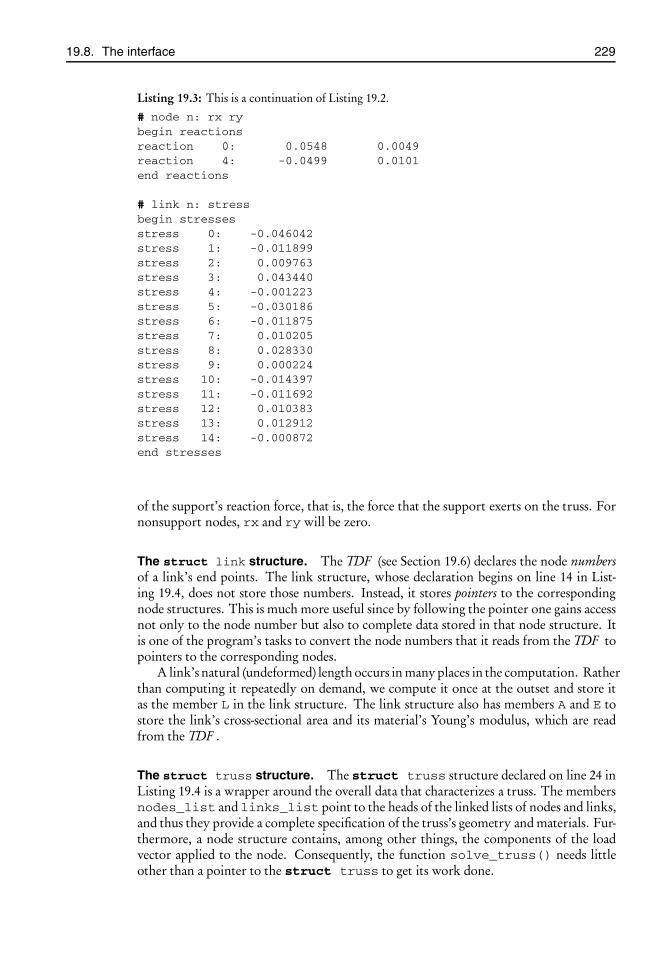
root2014/7/8page 229
�
�
�
�
�
�
�
�
19.8. The interface 229
Listing 19.3: This is a continuation of Listing 19.2.
# node n: rx rybegin reactionsreaction 0: 0.0548 0.0049reaction 4: -0.0499 0.0101end reactions
# link n: stressbegin stressesstress 0: -0.046042stress 1: -0.011899stress 2: 0.009763stress 3: 0.043440stress 4: -0.001223stress 5: -0.030186stress 6: -0.011875stress 7: 0.010205stress 8: 0.028330stress 9: 0.000224stress 10: -0.014397stress 11: -0.011692stress 12: 0.010383stress 13: 0.012912stress 14: -0.000872end stresses
of the support’s reaction force, that is, the force that the support exerts on the truss. Fornonsupport nodes, rx and ry will be zero.
The struct link structure. The TDF (see Section 19.6) declares the node numbersof a link’s end points. The link structure, whose declaration begins on line 14 in List-ing 19.4, does not store those numbers. Instead, it stores pointers to the correspondingnode structures. This is much more useful since by following the pointer one gains accessnot only to the node number but also to complete data stored in that node structure. Itis one of the program’s tasks to convert the node numbers that it reads from the TDF topointers to the corresponding nodes.
A link’s natural (undeformed) length occurs in many places in the computation. Ratherthan computing it repeatedly on demand, we compute it once at the outset and store itas the member L in the link structure. The link structure also has members A and E tostore the link’s cross-sectional area and its material’s Young’s modulus, which are readfrom the TDF .
The struct truss structure. The struct truss structure declared on line 24 inListing 19.4 is a wrapper around the overall data that characterizes a truss. The membersnodes_list and links_list point to the heads of the linked lists of nodes and links,and thus they provide a complete specification of the truss’s geometry and materials. Fur-thermore, a node structure contains, among other things, the components of the loadvector applied to the node. Consequently, the function solve_truss() needs littleother than a pointer to the struct truss to get its work done.
root2014/7/8page 230
�
�
�
�
�
�
�
�
230 Chapter 19. Trusses
Listing 19.4: The header file truss.h.
1 #ifndef H_TRUSS_H2 #define H_TRUSS_H3 #include "linked-list.h"4
5 struct node {6 int n; // node number7 double X, Y; // node coordinates before deformation8 double x, y; // node coordinates after deformation9 int xfixed, yfixed; // true if coord is constrained
10 double fx, fy; // components of the applied load11 double rx, ry; // components of reaction at support, if any12 };13
14 struct link {15 int n; // link number16 struct node *np1; // pointer to node at one end17 struct node *np2; // pointer to node at the other end18 double L; // link’s natural length19 double A; // link’s cross-sectional area20 double E; // the Young’s modulus21 double stress; // link’s stress22 };23
24 struct truss {25 conscell *nodes_list; // linked list of nodes26 conscell *links_list; // lined list of links27 int nnodes; // number of nodes28 int nlinks; // number of links29 };30
31 int solve_truss(struct truss *truss,32 double h, double tol, int maxevals);33
34 #endif /∗ H_TRUSS_H */
The function solve_truss(). The function solve_truss()whose prototype ap-pears on line 31 in Listing 19.4 receives a pointer to a truss structure and calculates itsdeformation by searching for a minimizer of the energy. It passes arguments h, tol, andmaxevals to nelder_mead(), which actually performs the minimization. The con-figuration data of the deformed truss is printed to the stdout in a format compatiblewith a TDF . The function returns true upon success and false if anything goes wrong.Diagnostics are printed to the stderr.
19.9 Reading and writing: truss-io.[ch]The task of reading and parsing a TDF is sufficiently complex to warrant isolating it intoa separate file truss-io.c with an associated header file truss-io.h.
In fact, truss-io.c makes up the bulk of the program. In my implementation it is 332lines long, while the solver itself (in file truss.c, more on that later) is only 177 lines long.Despite that length, the interface truss-io.h, shown in Listing 19.5, is quite simple.

root2014/7/8page 231
�
�
�
�
�
�
�
�
19.9. Reading and writing: truss-io.[ch] 231
Listing 19.5: The file truss-io.h.
1 #ifndef H_TRUSS_IO_H2 #define H_TRUSS_IO_H3 #include <stdio.h>4 #include "truss.h"5 struct truss *read_truss(FILE *stream);6 void write_truss(struct truss *truss);7 void free_truss(struct truss *truss);8 #endif /∗ H_TRUSS_IO_H */
The function read_truss() reads a TDF from an input stream, aggregates the in-formation into a truss structure, and returns a pointer to that structure. It allocates mem-ory for the various structures as needed. Its sole argument, stream, is the stream fromwhich it is to read the data. Our program invokes read_truss() with stream set tostdin, although other streams may be used equally well.
The function write_truss() acts almost as the inverse of read_truss(). Itwrites the data of the deformed truss to the stdout in a format consistent with the TDFspecifications. It would be a trivial change to make it write to an arbitrary output streamrather than to the stdout, as done in read_truss(). You may do it that way if youwish.
The function free_truss() receives a pointer to a truss structure and frees thememory resources previously allocated by read_truss(). Normally you will callfree_truss() at the end of the computation, just before exiting.
In addition to these three functions with external linkage, the file truss-io.c contains10 functions with internal linkage, i.e., specified static. Listing 19.6 shows an outlineof truss-io.c. I will describe its details in the following subsections.
19.9.1 The function read_truss()
The function read_truss() that appears on line 34 of Listing 19.6 is the controllingfunction of most of the rest of the file truss-io.c, and it has a big job to do. Nevertheless,it is quite clean and straightforward, as it delegates the messy work to the other func-tions. Its objective is to read a TDF from the specified stream, store the information in astruct truss, and return that structure’s address. Listing 19.7 shows the contents ofthe function read_truss() in its entirety. Let’s go through it line by line.
In the first few lines it declares a pointer to the truss structure that it’s going to con-struct, as well as pointers to the linked lists of the truss’s nodes and links. The variablelineno is initialized at 0; it will be incremented upon reading the input stream’s succes-sive lines. Its purpose is to help the program issue helpful diagnostic messages, completewith line numbers, when problems occur in the input. There’s not much use in saying“there is an error somewhere” without saying where.
After these initial preparations, the function commences to read, on line 8, the TDF ’snode specifications section since that is the first section in a TDF . Actually, it delegates thetask to the function get_nodes() which specializes in reading a TDF ’s nodes. We willsee the details of the implementation of get_nodes() in subsection 19.9.2. What weneed to know at this stage is that upon success, get_nodes() constructs and returns alinked list of node structures that carries the information extracted from the TDF ’s nodessection.
If get_nodes() fails for some reason, e.g., due to incomplete or garbled data, it freeswhatever memory it has allocated in its aborted attempt and returns NULL. In that case
root2014/7/8page 232
�
�
�
�
�
�
�
�
232 Chapter 19. Trusses
Listing 19.6: An outline of the file truss-io.c.
1 #include <stdio.h>2 #include <string.h>3 #include <math.h>4 #include "linked-list.h"5 #include "fetch-line.h"6 #include "xmalloc.h"7 #include "truss.h"8 #include "truss-io.h"9 #define BUFLEN 128
10 #define SQ(x) ((x)*(x))11
12 // functions for reading nodes13 � static void free_nodes_list(conscell *nodes) ...14 � static struct node *make_node(int n, double x, double y,15 int xfixed, int yfixed) ...16 � static struct node *process_node_line(char *str) ...17 � static conscell *get_nodes(FILE *stream, int *lineno) ...18
19 // functions for reading links20 � static void free_links_list(conscell *links) ...21 � static struct link *make_link(int n, int n1, int n2,22 double A, double E, conscell *nodes_list) ...23 � static struct link *process_link_line(char *str,24 conscell *nodes_list) ...25 � static conscell *get_links(FILE *stream, int *lineno,26 conscell *nodes_list) ...27
28 // functions for reading loads29 � static int process_load_line(char *str, conscell *nodes_list) ...30 � static int get_loads(FILE *stream, int *lineno,31 conscell *nodes_list) ...32
33 // functions with external linkage34 � struct truss *read_truss(FILE *stream) ...35 � void write_truss(struct truss *truss) ...36 � void free_truss(struct truss *truss) ...
the if (...) test on line 8 halts the function read_truss() and returns NULL tothe caller.
If the reading of the nodes section is successful, control transfers to line 10, whereanother specialized function, get_links(), is called to read the TDF ’s links section.If successful, get_links() constructs and returns a linked list of link structures thatcarries the information extracted from the TDF ’s links section. Otherwise it frees what-ever memory it has allocated in the process and returns NULL. In that case theif (...)test on line 10 halts the function read_truss(), but before returning NULL to thecaller, it dutifully frees the memory associated with the linked list of nodes which it hadobtained earlier.
The next segment, beginning on line 15, calls the function get_loads(), which spe-cializes in reading a TDF ’s loads section. Unlike the previous two segments, this functiondoes not return a linked list. It simply reads the loads vectors from the TDF and inserts

root2014/7/8page 233
�
�
�
�
�
�
�
�
19.9. Reading and writing: truss-io.[ch] 233
Listing 19.7: The function read_truss() in the file truss-io.c. It reads a TDF from the stream,stores the information in a struct truss, and returns that structure’s address.
1 struct truss *read_truss(FILE *stream)2 {3 struct truss *truss;4 conscell *nodes_list;5 conscell *links_list;6 int lineno = 0;7
8 if ((nodes_list = get_nodes(stream, &lineno)) == NULL)9 return NULL;
10 if ((links_list = get_links(stream, &lineno, nodes_list))11 == NULL) {12 free_nodes_list(nodes_list);13 return NULL;14 }15 if (!get_loads(stream, &lineno, nodes_list)) {16 free_nodes_list(nodes_list);17 free_links_list(links_list);18 return NULL;19 }20
21 nodes_list = ll_reverse(nodes_list);22 links_list = ll_reverse(links_list);23
24 truss = xmalloc(sizeof *truss);25 truss→nodes_list = nodes_list;26 truss→links_list = links_list;27 truss→nnodes = ll_length(nodes_list);28 truss→nlinks = ll_length(links_list);29 fprintf(stderr, "read %d nodes, %d links\n",30 truss→nnodes, truss→nlinks);31 return truss;32 }
them into the corresponding nodes. That’s the reason why it receives the linked list ofnodes as an argument. If the reading is successful, it returns true; otherwise it returns false.In the latter case, the if (...) test on line 15 halts the function read_truss(), butbefore returning NULL to the caller, it dutifully frees the memory associated with thelinked lists of nodes and links which had been constructed earlier.
If the reading of the TDF ends with success, control is transferred to line 21, wherethe function ll_reverse() from Chapter 16 is called to reverse the order of the nodeslist. This is by no means necessary, but it’s desirable: A linked list is assembled by pushingsuccessive links into the head of the list, so it ends up in the reverse order of the arrival ofthe items. Without the reversal, the nodes in the program’s output will be printed in thereverse order of the input. Line 22 serves a similar purpose in relation to the linked listof links.
At this point success is at hand. We call xmalloc() to allocate memory for a trussstructure, hang the linked lists of nodes and links on it, print a informational message (tothe stderr) announcing the number of nodes and links read, and return the address ofthe truss structure to the caller.

root2014/7/8page 234
�
�
�
�
�
�
�
�
234 Chapter 19. Trusses
Listing 19.8: The function get_nodes() in the file truss-io.c. It is responsible for reading thenodes section of a TDF . The preprocessor macro BUFLEN is defined on line 9 inListing 19.6 on page 232.
1 static conscell *get_nodes(FILE *stream, int *lineno)2 {3 conscell *nodes_list = NULL; // an empty list4 struct node *node;5 char buf[BUFLEN];6 char *str;7 if ((str = fetch_line(buf, BUFLEN, stream, lineno)) == NULL) {8 fprintf(stderr, "*** error: no node data in input\n");9 return NULL;
10 }11 if (strcmp(str, "begin nodes") �= 0) {12 fprintf(stderr, "*** error: no ‘begin nodes’ in input\n");13 return NULL;14 }15 while ((str = fetch_line(buf, BUFLEN, stream, lineno)) �= NULL) {16 if (strcmp(str, "end nodes") == 0)17 return nodes_list;18 if ((node = process_node_line(str)) == NULL) {19 fprintf(stderr, "*** error: bad syntax on input line %d\n",20 *lineno);21 free_nodes_list(nodes_list);22 return NULL;23 }24 nodes_list = ll_push(nodes_list, node);25 }26 fprintf(stderr, "*** error: no ‘end nodes’ in input\n");27 free_nodes_list(nodes_list);28 return NULL;29 }
Remark 19.3. Normally the user will redirect the program’s stdout to a file to capturethe solution’s data. That informational message noted above is not a part of the solution,so we print it to the stderr, which will flow to the screen and catch the user’s attention,as explained in Chapter 3. The moral of the story: stderr is not exclusively for errormessages.
19.9.2 The function get_nodes()
The function get_nodes() that appears on line 17 of Listing 19.6 on page 232 is respon-sible for reading the nodes section of a TDF . As we saw in subsection 19.9.1, it constructsand returns a linked list of node structures carrying the information extracted from theTDF .
In Listing 19.8 I have shown the function in its entirety, not because it’s particularlylong or complex, but because its gingerly, almost paranoiac, manner of stepping throughthe TDF sets the tone for the several similar functions which we will encounter.
It begins with defining an empty linked list called nodes_list, and it sets up a char-acter buffer buf[BUFLEN], which will hold successive lines read from the TDF through

root2014/7/8page 235
�
�
�
�
�
�
�
�
19.9. Reading and writing: truss-io.[ch] 235
calls to fetch_line(). The preprocessor macro BUFLEN is defined on line 9 in List-ing 19.6 on page 232.
The first call to fetch_line() occurs on line 7. The expectation here is to findthe string “begin nodes”, which announces the beginning of the TDF ’s nodes section; seeSection 19.6 for the details of a TDF . If input ends before fetch_line() finds any-thing substantive—remember that fetch_line() skips over blanks and comments—fetch_line() returnsNULL, in which caseget_nodes() issues a diagnostic on line 8and returns NULL to the caller.
On the other hand, if fetch_line() returns non-NULL, then control transfers toline 11, where the fetched string is compared against the target “begin nodes” with the helpof the standard library’s strcmp(). The latter returns zero if the stings exactly match,and nonzero otherwise.75 If the comparison fails, get_nodes() issues a diagnostic online 12 and returns NULL to the caller.76
If the string “begin nodes” is found, we expect that the subsequent lines will be eithernode specifications or the “end nodes” string. The while-loop that spans lines 15–25repeatedly calls fetch_line() to extract, examine, and processes successive lines fromthe TDF .
Line 16 compares the fetched string against “end nodes”. If it’s a match, the nodessection has ended and the function’s job is finished. The pointer nodes_list, whichpoints to the head of the linked list of the nodes, is returned to the caller.
Otherwise, the helper function process_node_line() is called on line 18 to pro-cess the string. We will see the details of that function in the next subsection. What weneed to know at the moment is that if the string is malformed, it rejects it and returnsNULL, in which case a diagnostic message is printed (line 19), the linked list constructedthus far is freed, and get_nodes() returns NULL. If the string is well formed, however,it extracts the node number and the node’s coordinates from the string, allocates memoryfor a node structure, inserts the extracted values in it, and returns that node’s address. Online 24 the new node is pushed into the linked list of nodes, and then the while-looprepeats.
The normal return from the function get_nodes() is from line 17, which happenswhen the string “end nodes” is reached. If that string is missing, the while-loop falls offits end and the control transfers to line 26, where an appropriate diagnostic is printed, thelinked list of nodes is freed, and get_nodes() returns NULL.
19.9.3 The function process_node_line()
The function process_node_line() appearing on line 16 of Listing 19.6 on page 232receives a string as an argument which is expected to be a node specification line from aTDF . If the string meets the expectation, it allocates a struct node, fills in the node’smembers with data that it extracts from the string, and returns the node’s address to thecaller. If the string is malformed, it returns NULL.
The first task of process_node_line() is to decide which of the four types ofnode specifications listed on page 226 it has received. They are different only by theplacement of the asterisks that indicate immobile coordinates. Thus, a string of the form“node n: x *y” specifies a node whose y coordinate is fixed but the x coordinate is
75Here we rely on the proper functioning of our fetch_line() function, which is designed to removeboth leading and trailing spaces from a string. An errant whitespace here will foul up the comparison.
76Perhaps that diagnostic is too cryptic. It could be made more explicit by saying something likefprintf(stderr, Expected ‘begin nodes’but found %s on line %d\n",
str, *lineno);

root2014/7/8page 236
�
�
�
�
�
�
�
�
236 Chapter 19. Trusses
Listing 19.9: This fragment of the function process_node_line() (in the file truss-io.c) scansa string for one of the four possible input types listed on page 226. You will add codeto handle the other three types. If the string fails to match one of the four types, thefunction returns NULL.
1 static struct node *process_node_line(char *str)2 {3 double x, y;4 int n;5 if (sscanf(str, "node %d: %lf %lf", &n, &x, &y) == 3)6 return make_node(n, x, y, 0, 0);7 else if (sscanf(str, "node %d: *%lf %lf", &n, &x, &y) == 3)8 ...9 else
10 return NULL;11 }
Listing 19.10: The function make_node() in the file truss-io.c.
1 static struct node *make_node(int n, double x, double y,2 int xfixed, int yfixed)3 {4 struct node *node = xmalloc(sizeof *node);5 node→n = n;6 node→X = node→x = x;7 node→Y = node→y = y;8 node→xfixed = xfixed;9 node→yfixed = yfixed;
10 node→fx = node→fy = 0.0;11 node→rx = node→ry = 0.0;12 return node;13 }
free to move (it’s a horizontal roller support). Consequently, in the corresponding nodestructure (see Listing 19.4 on page 230) it should set xfixed = 0 and yfixed = 1.
Our process_node_line() delegates the creation of the node structure and set-ting the values of its various members to yet another helper function, make_node().We will examine the details of make_node() in the next subsection. What we needto know at the moment is that it receives the values of n, x, y, xfixed, and yfixed asarguments; then it allocates memory for astruct node, fills in those five values, and re-turns that node’s address. Equipped with that knowledge, you should be able to completethe function process_node_line(), a fragment of which is shown in Listing 19.9.
19.9.4 The function make_node()
The function make_node() that appears on line 14 of Listing 19.6 on page 232 allocatesmemory for a node structure and fills the values of the n, x, y, xfixed, and yfixedmembers with those that it receives as arguments. Listing 19.10 shows its implementation.As you see, it does more than just filling in the five members.
For one thing, on lines 6 and 7 it sets the node’s undeformed coordinates (X,Y),as well as the deformed coordinates (x,y), to the values received (which are the values

root2014/7/8page 237
�
�
�
�
�
�
�
�
19.9. Reading and writing: truss-io.[ch] 237
read from the TDF ). In subsection 19.12.6 we will see that the truss solver constructs theNelder–Mead initial simplex from the values stored in the (x,y) coordinates. Conse-quently, the search for the minimum energy begins from the truss’s undeformed state. InPart 19.5 of this chapter’s Projects section we will also see that the user has the opportunityto override this default choice if he/she so wishes.
For another thing, the load vector components fx and fy are set to zero as defaults.These may be overwritten later when the program reads the loads section of the TDF .If a node is not mentioned in that section, the default values remain in effect.
Finally, the support reaction force components, rx and ry, are set to zero as defaults.They will remain zero for nonsupport nodes. The reaction forces at the support nodeswill be calculated and updated after the truss is solved.
Remark 19.4. This ends the chain of function that collectively read a TDF ’s nodedescription section. Each function delegates the details of a complex task to the next“specialist” function:
read_truss() � get_nodes() � process_node_line() � make_node()
Such a division of labor helps to make the logic of the program transparent and avoidsexcessively long and complex functions which may be difficult to comprehend and debug.
19.9.5 The function free_nodes_list()
The function free_nodes_list() that appears on line 13 of Listing 19.6 on page 232frees all memory resources associated with a linked list of nodes. Merely applying Chap-ter 16’s ll_free() won’t suffice since that frees only the memory associated with thecons cells, but the data members of the cons cells point to node structures which alsotake up memory. Therefore, free_nodes_list() should traverse the linked list andfree those node structures first, and only then apply ll_free() to free the cons cells.I leave it to you to implement free_nodes_list().
Normallyfree_nodes_list() is called when the program has completed its workwith the analysis of the truss—probably just before it exits—but there are other occasionsfor it as well. For instance, it is called on line 21 of Listing 19.8 (page 234) to free a partiallybuilt list when errors are encountered during the reading of the TDF .
19.9.6 Reading a TDF ’s links section
The functions on lines 20–25 of Listing 19.6 (page 232) are devoted to reading a TDF ’slinks section much in the same way that the functions on lines 13–17 were devoted toreading the nodes section. The chain of the function calls is similar:
read_truss() � get_links() � process_link_line() � make_link()
The differences between the link and node reading functions are slight; therefore there isno point in repeating what has been said in subsections 19.9.2 through 19.9.5. I will limitmy comments to pointing out a few differences.
The functions free_links_list() and get_links() basically are copies ofthe functions free_nodes_list() and get_nodes(), where all occurrences of“node” change to “link”. Note, however, unlike get_nodes(), get_links() receivesa pointer to the linked list of nodes. It has no direct use for that linked list itself; it merelypasses it to process_link_line(), which in turn passes it to make_link(), whichneeds it for assigning node pointers to the link’s endpoints. Once make_link() de-termines those endpoints, it extracts the node coordinates (X1,Y1) and (X2,Y2) of the
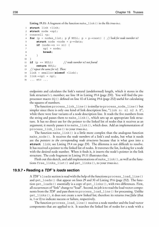
root2014/7/8page 238
�
�
�
�
�
�
�
�
238 Chapter 19. Trusses
Listing 19.11: A fragment of the function make_link() in the file truss-io.c.
1 struct link *link;2 struct node *np1;3 conscell *p;4 for (p = nodes_list; p �= NULL; p = p→next) { // look for node number n15 struct node *node = p→data;6 if (node→n == n1) {7 np1 = node;8 break;9 }
10 }11 if (p == NULL) // node number n1 not found12 return NULL;13 // repeat the same for n2. Then:14 link = xmalloc(sizeof *link);15 link→np1 = np1;16 ... etc ...
endpoints and calculates the link’s natural (undeformed) length, which it stores in thelink structure’s L member; see line 18 in Listing 19.4 (page 230). You will find the pre-processor macro SQ() defined on line 10 of Listing 19.6 (page 232) useful for calculatingthe squares of numbers.
The function process_link_line() is similar toprocess_node_line() butsimpler since there is only one kind of link description line, “link n: n1 n2 A E”,while there were four variants of a node description line. It reads the five numbers fromthe string and passes them to make_link(), which sets up an appropriate link struc-ture. It has no direct use for the pointer to the linked list of nodes that it receives as anargument; it merely passes it to make_link(), which does. Add an implementation ofprocess_link_line() to your truss-io.c.
The function make_link() is a little more complex than the analogous functionmake_node(). It receives the node numbers of a link’s end nodes, but what it needsare the pointers to the corresponding node structures because that is what goes into astruct link; see Listing 19.4 on page 230. The dilemma is not difficult to resolve.It has received a pointer to the linked list of nodes. It traverses the list, looking for a nodewith the desired node number. When it finds it, it inserts the node’s pointer in the linkstructure. The code fragment in Listing 19.11 illustrates that.
Flesh out this sketch, and add implementations of make_link(), as well as the func-tions free_links_list() and get_links(), to your truss-io.c.
19.9.7 Reading a TDF ’s loads section
A TDF ’s loads section is read with the help of the functions process_load_line()and get_loads() that appear on lines 29 and 30 of Listing 19.6 (page 232). The func-tion get_loads() essentially is a copy of get_links(), with two differences. First,all occurrences of “link” change to “load”. Second, its job is to read the load vector compo-nents from the TDF and pass them to process_load_line() for processing. Unlikeget_links(), it does not create a new linked list; therefore its returns true/false (thatis, 1 or 0) to indicate success or failure, respectively.
The function process_load_line() receives a node number and the load vectorcomponents that are applied to it. It searches the linked list of nodes for a node with a

root2014/7/8page 239
�
�
�
�
�
�
�
�
19.9. Reading and writing: truss-io.[ch] 239
matching node number and deposits the components of the load vector in the node’s fxand fy members, and then it returns 1 (true). If a node with the given node number doesnot exist (this indicates an error in the TDF ), it returns 0 (false). The search for the nodeis performed exactly like that in make_link().
Add your implementation of process_load_line() andget_loads() to yourtruss-io.c.
This concludes the description of the details of read_truss() and its ancillaryfunctions.
19.9.8 The function write_truss()
The function write_truss() that appears on line 35 of Listing 19.6 (page 232) is calledafter the truss solver (described later) has done its job of determining the truss’s deforma-tion. It writes to the solution to the stdout in a form conforming to the format of aTDF , followed by extra data that give stresses in the links and reaction forces at the sup-ports. Listing 19.2 on page 228 (continued into Listing 19.3 on the next page) shows theoutput corresponding to the TDF Cantilever.tdf of Section 19.6.
The first part of the output, that shown in Listing 19.2, consists of the usual three sec-tions of a TDF . In fact, the contents of the links and loads sections are identical—ignoringthe cosmetic formatting differences—to those of the input file because link connectivityand applied loads are no different before and after. The contents of the nodes section, how-ever, are very different; the coordinates here are those of the truss’s deformed state. I usedthose coordinates to draw (manually) the deformed shape in Figure 19.6 on page 222.Those same coordinates are used by the truss_to_eps() function of Section 19.10 toautomatically generate the drawing shown in Figure 19.10 on page 249.
Remark 19.5. As is noted in the caption of Listing 19.2, the placements of the aster-isks against the nodes 0 and 4 are quite different from those seen in the (manually typed)Cantilever.tdf, where the asterisks are attached to the respective x and y coordinate val-ues. It is possible to achieve a similar effect on the output; however, the extra work is notworth the effort, so I have left it as it is. Despite that annoying difference, the result stillconforms to the TDF specifications since sscanf() ignores extra whitespace.
The continuation of the output in Listing 19.3 shows additional data regarding thetruss’s state. The section between “begin reactions” and “end reactions” contains linesof the form reaction n: rx ry, where n is a node number, and rx and ry are thecomponents of the support reaction at that node. A support reaction is the force exertedby the support on the truss. Only the support nodes are listed. The calculation of thesupport reactions is the subject of subsection 19.12.4.
The section between “begin stresses” and “end stresses” contains lines of the formstress n: s, where n is a link number and s is the stress in that link. This is crucialinformation for truss design—excessive stress will make a link buckle or snap. We will seehow to compute the stresses in subsection 19.12.3.
19.9.9 The function free_truss()
The function free_truss() that appears on line 36 of Listing 19.6 (page 232) is respon-sible for freeing all the allocated memory associated with the truss. That memory consistsof those of the linked list of the nodes, the linked list of the links, and the truss structureitself. We already have functions to free up the linked lists; therefore the implementationof free_truss() is quite trivial:

root2014/7/8page 240
�
�
�
�
�
�
�
�
240 Chapter 19. Trusses
-0.00e+00
0.00e+00
com
pres
sion
tens
ion
0
0 1 2 3
4 5 6 7
0
1
2
3
4
5
6
7
8
9
10
11
12
13
14
-0.00e+00
0.00e+00
com
pres
sion
tens
ion
0
Figure 19.8: Two images of the truss Cantilever.tdf (see Section 19.6) in its referenceconfiguration produced by truss_to_eps(). The labels in the bottomfigure are produced by giving the TR_PLOT_WITH_LABELS option in thefunction’s third argument.
1 void free_truss(struct truss *truss)2 {3 if (truss �= NULL) {4 free_nodes_list(truss→nodes_list);5 free_links_list(truss→links_list);6 free(truss);7 }8 }
The check against NULL makes it safe to call free_truss() with a NULL argu-ment. This is consistent with the standard library’s free() function, as well as all otherfree_*() functions in this book, which handle a NULL gracefully.
Add this implementation of free_truss() to your truss-io.c.
19.10 The files truss-to-eps.[ch]I have written a function named truss_to_eps() with the prototype
void truss_to_eps(struct truss *truss, char *epsfile, int labels);
which receives a pointer to a struct truss, from which it extracts the informationnecessary for drawing an image of the loaded truss, in the EPS format, into a file whosename is specified in the epsfile argument. The image depicts the truss, the supports,and the load vectors. The third argument must be one of
TR_PLOT_WITH_NO_LABELS or TR_PLOT_WITH_LABELS
If the TR_PLOT_WITH_LABELS is given, the node and link numbers are drawn on theimage as well. Figure 19.8 shows images of the truss Cantilever.tdf (see Section 19.6) in itsreference configuration, with and without labels, produced by truss_to_eps(). Thedeformed image of that same truss is shown in Figure 19.10 on page 249.

root2014/7/8page 241
�
�
�
�
�
�
�
�
19.11. Interlude (and a mini-project) 241
Listing 19.12: The file interlude.c is a simple driver for testing the read_truss() andwrite_truss() functions.
1 #include <stdlib.h>2 #include "truss-to-eps.h"3 #include "truss-io.h"4 #include "truss.h"5 int main(void)6 {7 struct truss *truss;8 if ((truss = read_truss(stdin)) == NULL)9 return EXIT_FAILURE;
10 truss_to_eps(truss, "z-with-labels.eps", TR_PLOT_WITH_LABELS);11 truss_to_eps(truss, "z-without-labels.eps", TR_PLOT_WITH_NO_LABELS);12 write_truss(truss);13 free_truss(truss);14 return EXIT_SUCCESS;15 }
Links are drawn in colors that represent the magnitudes of stress in them. Compres-sion is shown in dark red, tension in dark blue, and neutral (zero or almost zero stress) inlight green. A color scale accompanying the drawing shows the correspondence betweenthe stress and the varying hues.
The function truss_to_eps() consults the values of the (lowercase) (x,y) nodecoordinates77 to draw the truss. It follows that the resulting image corresponds to thetruss’s undeformed shape if truss_to_eps() is called before solving the truss and thedeformed shape if called after.
Implementing the function truss_to_eps() is not a part of this project becausethat requires some familiarity with the PostScript language, which I don’t want to make aprerequisite for this book. You should download my implementation of the files world-to-eps.c and world-to-eps.h from this book’s website, drop them in this project’s directory,and compile them along with the rest of your files.
19.11 Interlude (and a mini-project)At this point we have functions to read and write a TDF . It’s a good idea to stop for amoment and test those before we move on.
The file interlude.c shown in Listing 19.12 is a simple and self-explanatory driver fortesting your read_truss() and write_truss() functions. Compile and link witheverything else that it depends on to produce an executable named interlude, and thenrun it:
$ ./interlude <Cantilever.tdf >Cantilever.out
where Cantilever.tdf is as in Section 19.6. If your program works correctly, its outputshould agree with the Cantilever.tdf modulo cosmetic differences. Additionally, it willproduce two EPS files named z-with-labels.eps and z-without-labels.eps which you may viewwith any PostScript viewer. Figure 19.8 shows the results.
For further testing, copy Cantilever.tdf to a temporary file, say tmp.tdf, introducedeliberate errors of various sorts in it, and verify that your program catches them.
77See subsection 19.12.6 for an explanation of the distinction between the (x,y) and (X,Y) coordinates.

root2014/7/8page 242
�
�
�
�
�
�
�
�
242 Chapter 19. Trusses
Listing 19.13: An outline of the file truss.c.
1 #include <stdio.h>2 #include <math.h>3 #include "linked-list.h"4 #include "array.h"5 #include "nelder-mead.h"6 #include "truss.h"7 #define SQ(x) ((x)*(x))8 � static double stress_function(double lambda) ...9 � static double stored_energy_function(double lambda) ...
10 � static double link_stretch(struct link *link) ...11 � static void evaluate_stresses(struct truss *truss) ...12 � static void evaluate_reactions(struct truss *truss) ...13 � static double total_energy(double *x, int n, void *params) ...14 � int solve_truss(struct truss *truss,15 double h, double tol, int maxevals) ...
19.12 The file truss.cThe file truss.c defines the function solve_truss(), which provides the primary userinterface to our truss solving utility. Listing 19.13 shows an outline of truss.c. Six ancillaryfunctions (lines 8–13) with internal linkage provide support to solve_truss(). I willexplains the purposes of each of those functions in the following subsections.
19.12.1 The stress_function() and stored_energy_function()
The functions stress_function() and stored_energy_function() that ap-pear on lines 8 and 9 of Listing 19.13 evaluate the template functions �σ(λ) and �W (λ)defined in equations (19.10) on page 226. Add your implementations of these to yourtruss.c.
19.12.2 The function link_stretch()
The functionlink_stretch() that appears on line 10 of Listing 19.13 receives a pointerto a link structure and calculates the link’s stretch λ, which, as defined in subsection 19.2.1,is the ratio of the link’s deformed and reference lengths.
Since a link structure contains pointers to the nodes at the link’s endpoints, you mayfollow those pointers to access the coordinates (x,y) of those nodes and thus calculatethe link’s deformed length through the usual formula
�(x2− x1)
2+(y2− y1)2. You will
find the preprocessor macro SQ() defined on line 7 of Listing 19.13 useful for calculat-ing squares of numbers. You won’t need to calculate the link’s length in the referenceconfiguration—that length is available in the member L of the link structure.
Add your implementation of link_stretch() to your truss.c.
19.12.3 The function evaluate_stresses()
The function evaluate_stresses() that appears on line 11 of Listing 19.13 walksthrough the truss’s linked list of links, calculates the stress in each link, and stores itin the link structure’s stress member. According to (19.10), the stress is σ = E�σ(λ).The values of λ and �σ(λ) are computed by calling the functions link_stretch() and

root2014/7/8page 243
�
�
�
�
�
�
�
�
19.12. The file truss.c 243
x j
−→−→F
i j
−→←−F i
xi
Figure 19.9: Four links connect to, and exert forces on, the support node xi . Addition-ally, an external load of F i is applied directly to the node. The support’sreaction is equal and opposite to the vector sum of the forces.
stress_function(). The value of Young’s modulus E is available as the link struc-ture’s E member.
Add your implementation of evaluate_stresses() to your truss.c.
19.12.4 The function evaluate_reactions()
The function evaluate_reactions() that appears on line 12 of Listing 19.13 com-putes the reactions at the support nodes. These are the forces that the supports exert onthe truss.
Figure 19.9 shows a support node xi (marked by a triangle) and the four links78 thatconnect to it. In addition to the forces exerted through the links, an external force,F i , is applied directory to the node.
The link that connects the node xi to another node, x j , exerts a force of magnitudeAi jσ(λi j ) on the support, where Ai j is that link’s cross-sectional area and λi j is its stretch.The force vector, which is directed along the link as shown in the figure, is given by
F i j =Ai jσ(λi j )x j −xi
‖x j −xi‖ . (19.11)
The fraction in the expression above produces the unit vector along the link, directedfrom xi to x j . The support’s reaction Ri is equal and opposite the vector sum of all theforces exerted on it:
Ri =−*F i +
∑links to xi
F i j+.
You should be able to write your ownevaluate_reactions()now. Listing 19.14provides a sketch. Note that in summing the loads on lines 12 and 13 we rely onnode→rxand node→ry being initially zero, which is the case since these were zeroed in the func-tion make_node(); see subsection 19.9.4.
Add your implementation of evaluate_reactions() to truss.c.
19.12.5 The function total_energy()
The function total_energy() that appears on line 13 of Listing 19.13 implementsthe energy of the truss, � (x0,x1, . . . ,xn−1), defined in (19.9) on page 222. It is shown inSection 19.5 that a minimizer of � corresponds to an equilibrium position of the truss.
78The choice of four links is for illustration only. The number of the links is immaterial in the followingdiscussion.
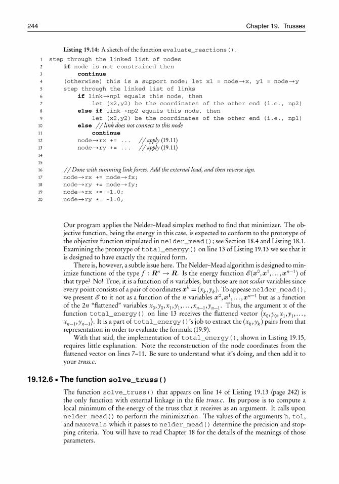
root2014/7/8page 244
�
�
�
�
�
�
�
�
244 Chapter 19. Trusses
Listing 19.14: A sketch of the function evaluate_reactions().
1 step through the linked list of nodes2 if node is not constrained then3 continue4 (otherwise) this is a support node; let x1 = node→x, y1 = node→y5 step through the linked list of links6 if link→np1 equals this node, then7 let (x2,y2) be the coordinates of the other end (i.e., np2)8 else if link→np2 equals this node, then9 let (x2,y2) be the coordinates of the other end (i.e., np1)
10 else // link does not connect to this node11 continue12 node→rx += ... // apply (19.11)13 node→ry += ... // apply (19.11)14
15
16 // Done with summing link forces. Add the external load, and then reverse sign.17 node→rx += node→fx;18 node→ry += node→fy;19 node→rx *= -1.0;20 node→ry *= -1.0;
Our program applies the Nelder–Mead simplex method to find that minimizer. The ob-jective function, being the energy in this case, is expected to conform to the prototype ofthe objective function stipulated in nelder_mead(); see Section 18.4 and Listing 18.1.Examining the prototype of total_energy() on line 13 of Listing 19.13 we see that itis designed to have exactly the required form.
There is, however, a subtle issue here. The Nelder–Mead algorithm is designed to min-imize functions of the type f : Rn → R. Is the energy function � (x0,x1, . . . ,xn−1) ofthat type? No! True, it is a function of n variables, but those are not scalar variables sinceevery point consists of a pair of coordinates xk = (xk , yk ). To appease nelder_mead(),we present � to it not as a function of the n variables x0,x1, . . . ,xn−1 but as a functionof the 2n “flattened” variables x0, y0, x1, y1, . . . , xn−1, yn−1. Thus, the argument x of thefunction total_energy() on line 13 receives the flattened vector ⟨x0, y0, x1, y1, . . . ,xn−1, yn−1⟩. It is a part of total_energy()’s job to extract the (xk , yk ) pairs from thatrepresentation in order to evaluate the formula (19.9).
With that said, the implementation of total_energy(), shown in Listing 19.15,requires little explanation. Note the reconstruction of the node coordinates from theflattened vector on lines 7–11. Be sure to understand what it’s doing, and then add it toyour truss.c.
19.12.6 The function solve_truss()
The function solve_truss() that appears on line 14 of Listing 19.13 (page 242) isthe only function with external linkage in the file truss.c. Its purpose is to compute alocal minimum of the energy of the truss that it receives as an argument. It calls uponnelder_mead() to perform the minimization. The values of the arguments h, tol,and maxevals which it passes to nelder_mead() determine the precision and stop-ping criteria. You will have to read Chapter 18 for the details of the meanings of thoseparameters.

root2014/7/8page 245
�
�
�
�
�
�
�
�
19.12. The file truss.c 245
Listing 19.15: The function total_energy() in the file truss.c evaluates the truss’s total en-ergy, � (x0,x1, . . . ,xn−1). The argument x is the flattened vector ⟨x0, y0, x1, y1, . . . ,xn−1, yn−1⟩.
1 static double total_energy(double *x, int n, void *params)2 {3 struct truss *truss = params;4 conscell *p;5 double e = 0.0;6 int j = 0;7 for (p = truss→nodes_list; p �= NULL; p = p→next) {8 struct node *node = p→data;9 node→x = x[j++];
10 node→y = x[j++];11 }12 for (p = truss→links_list; p �= NULL; p = p→next) {13 struct link *link = p→data;14 e += link→E * link→A * link→L15 * stored_energy_function(link_stretch(link));16 }17 for (p = truss→nodes_list; p �= NULL; p = p→next) {18 struct node *node = p→data;19 e -= (node→x - node→X) * node→fx20 + (node→y - node→Y) * node→fy;21 }22 return e;23 }
The position of the initial simplex is a crucial factor in determining the outcome ofthe Nelder–Mead iterations. If the objective function has multiple local minima, as doesa truss’s energy function in general, the algorithm is likely to converge to the local mini-mum that is closest to the starting point.
Our solver’s default choice for the initial simplex corresponds to the truss’s referenceconfiguration, but the user may override that default if so desired. To understand thisfully, we need to take a closer look at the role of a node’s coordinates.
Let us recall that thestruct node structure maintains two set of coordinates, (X,Y)and (x,y), for each node. The (X,Y) coordinates hold the node’s position in the truss’sreference configuration. These are assigned once and don’t change for the duration of theprogram. The (x,y) coordinates are initialized to (X,Y); see subsection 19.9.4. Afterthe truss is solved, they take on the values of the node’s deformed position.
The program builds the Nelder–Mead initial simplex based on the values of the (low-ercase) (x,y) coordinates. Since these are initialized to coincide with the (uppercase)(X,Y), the default initial simplex corresponds to the truss’s reference configuration.The user has the opportunity to alter the values of (x,y) at will between calls toread_truss() and solve_truss(), and thereby to set the initial simplex near adesired target position. See Part 19.4 in this chapter’s Projects section for an example.
Listing 19.16 shows my implementation of solve_truss(). Here I will commenton some of its more interesting features.
On line 6 the dimension N of the space is set to twice the number of nodes. This isbecause the objective function, that is, the energy, is a function of that many variables; seethe discussion about the “flattened” variables in the previous subsection.

root2014/7/8page 246
�
�
�
�
�
�
�
�
246 Chapter 19. Trusses
Listing 19.16: The function solve_truss() in the file truss.c.
1 int solve_truss(struct truss *truss, double h, double tol, int maxevals)2 {3 double **s;4 double *x;5 conscell *p;
6 int N = 2*truss→nnodes; // dimension of the energy space7 struct nelder_mead NM;8 int i, j, evalcount;9 make_vector(x, N);
10 for (j = 0, p = truss→nodes_list; p �= NULL; p = p→next) {11 struct node *node = p→data;12 x[j++] = node→x;13 x[j++] = node→y;14 }
15 make_matrix(s, N + 1, N); // the simplex matrix16 for (i = 0; i < N + 1 ; i++)17 for (j = 0; j < N; j++)18 s[i][j] = x[j];19 for (j = 0; j < N; j++)20 s[j+1][j] += h;
21 // project the simplex over the constraint space22 for (j = 0, p = truss→nodes_list; p �= NULL; p = p→next) {23 struct node *node = p→data;24 if (node→xfixed)25 for (i = 0; i < N + 1 ; i++)26 s[i][j] = node→X;27 j++;28 if (node→yfixed)29 for (i = 0; i < N + 1 ; i++)30 s[i][j] = node→Y;31 j++;32 }33 NM.f = total_energy;34 NM.n = N;35 NM.s = s;36 NM.x = x;37 NM.h = h;38 NM.tol = tol;39 NM.maxevals = maxevals;40 NM.params = truss;41 evalcount = nelder_mead(&NM);42 free_vector(x);43 free_matrix(s);44 if (evalcount > maxevals) {45 fprintf(stderr, "No convergence after %d "46 "function evaluation\n", evalcount);47 return 0;48 } else {49 fprintf(stderr, "Nelder-Mead converged after %d "50 "function evaluations\n", evalcount);51 evaluate_stresses(truss);52 evaluate_reactions(truss);53 return 1;54 }55 }
root2014/7/8page 247
�
�
�
�
�
�
�
�
19.13. The file truss-demo.c 247
Line 7 defines NM as an instance of a struct nelder_mead. This will bundle allthe information required for the minimization and pass that to nelder_mead() forprocessing.
The action begins on line 9, where a vector x of length N is created to serve as thecalculation’s independent variable. Recall that N is twice the number of nodes.
The for-loop on lines 10–14 flattens the energy function’s arguments—it traversesthe linked list of the truss’s nodes, reads the coordinates node→x and node→y of eachnode, and enters them as consecutive entries in the vector x.
Lines 15–20 create the (N+1) × N simplex matrix and populate its rows with copiesof the vector x first, and then they adjust them according to (18.5) on page 200 to form asimplex of size h.
The coordinates of some of the truss’s support nodes may be completely fixed (in ananchor node) or partially fixed (in a rolling node). Therefore, although the energy is afunction of N variables ⟨x0, y0, x1, y1, . . . , xn−1, yn−1⟩, not all of those variables are free tochange. Thus, the minimization of the energy takes place not on an N-dimensional space,but on an affine subspace defined by constraints of the form xk =�xk or yk =�xy , for certainindices k, where�xk and�xy are fixed.
Minimizing functions subject to affine constraints is explained in Section 18.8. Theoutcome of that section’s discussion is that if we project an arbitrary initial simplex ontothe constraint subspace, the Nelder–Mead algorithm will ensure that its subsequenceiterates remain within that subspace. Furthermore, Remark 18.9 on page 212 points outthat projecting onto constraint spaces of the form xk = �xk is particularly simple; it’s amatter of setting every entry in the corresponding column of the simplex matrix equalto�xk . This is precisely what is done on lines 22–32 of Listing 19.16. Examine that code,and make sure that you understand its details.
Now all is ready for calling the Nelder–Mead minimizer. On lines 33–40 we set upthe members of the NM structure; then on line 41 we pass the address of that structureto nelder_mead(). Once nelder_mead() returns, there is no longer a need for thevector x and matrix s, so we free them on lines 42 and 43.
There is a chance, of course, that Nelder–Mead fails to converge. We have designednelder_mead() so that it halts if the number of function evaluations exceeds the maxi-mum prescribed in maxevals. On line 44 we check the evaluation count againstmaxevals. If it is more, then we conclude that the algorithm hasn’t converged, so weprint a message to that effect to stderr and return 0, that is, false, to the caller. Other-wise, we print an a informative message regarding success (again, tostderr), then we callthe postprocessing functionsevaluate_stresses() andevaluate_reactions()to compute the stresses in the links and the reaction forces at the supports, and finally wereturn 1, that is, true, to the caller.
19.13 The file truss-demo.cThe file truss-demo.c shown in Listing 19.17 provides a driver for demonstrating, and ex-perimenting with, our truss solver. It is quite short, and much of it is self-explanatory;nevertheless, I will make a few comments on it.
Line 11. The function read_truss() is invoked to read a TDF from the stdin. Ifthe call fails, as it will if the TDF contains incomplete or inconsistent data, it returnsNULL, in which case the program exits with an EXIT_FAILURE status. We neednot print a message here since read_truss() prints its own diagnostics. If the
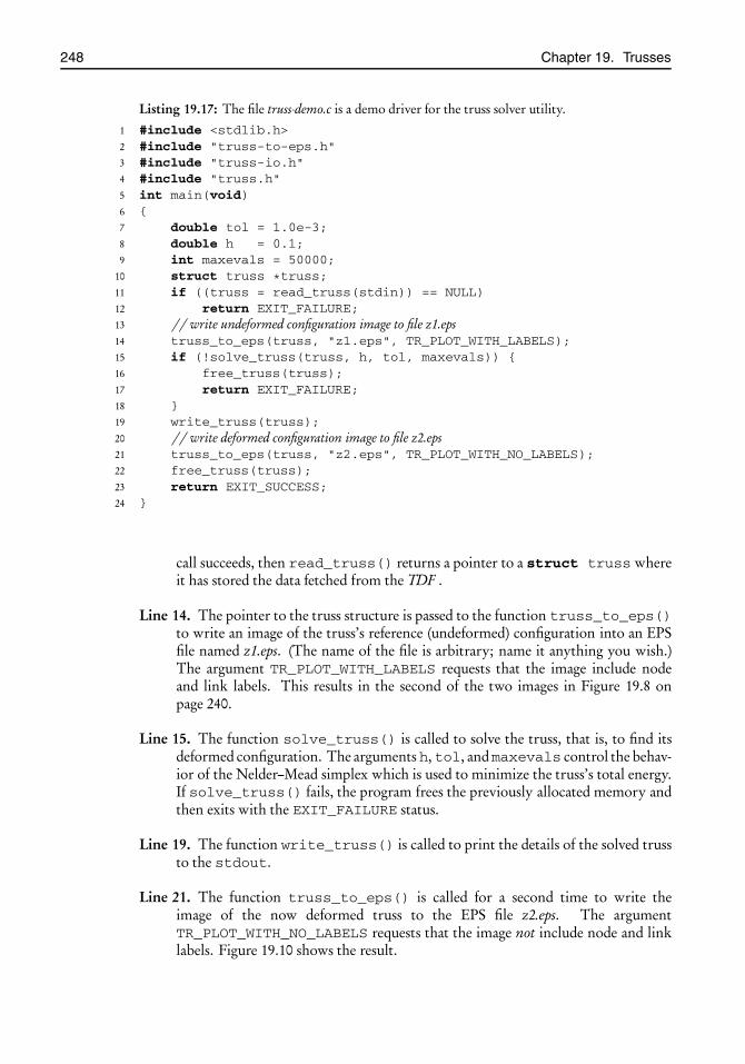
root2014/7/8page 248
�
�
�
�
�
�
�
�
248 Chapter 19. Trusses
Listing 19.17: The file truss-demo.c is a demo driver for the truss solver utility.
1 #include <stdlib.h>2 #include "truss-to-eps.h"3 #include "truss-io.h"4 #include "truss.h"5 int main(void)6 {7 double tol = 1.0e-3;8 double h = 0.1;9 int maxevals = 50000;
10 struct truss *truss;11 if ((truss = read_truss(stdin)) == NULL)12 return EXIT_FAILURE;13 // write undeformed configuration image to file z1.eps14 truss_to_eps(truss, "z1.eps", TR_PLOT_WITH_LABELS);15 if (!solve_truss(truss, h, tol, maxevals)) {16 free_truss(truss);17 return EXIT_FAILURE;18 }19 write_truss(truss);20 // write deformed configuration image to file z2.eps21 truss_to_eps(truss, "z2.eps", TR_PLOT_WITH_NO_LABELS);22 free_truss(truss);23 return EXIT_SUCCESS;24 }
call succeeds, then read_truss() returns a pointer to a struct truss whereit has stored the data fetched from the TDF .
Line 14. The pointer to the truss structure is passed to the function truss_to_eps()to write an image of the truss’s reference (undeformed) configuration into an EPSfile named z1.eps. (The name of the file is arbitrary; name it anything you wish.)The argument TR_PLOT_WITH_LABELS requests that the image include nodeand link labels. This results in the second of the two images in Figure 19.8 onpage 240.
Line 15. The function solve_truss() is called to solve the truss, that is, to find itsdeformed configuration. The arguments h, tol, andmaxevals control the behav-ior of the Nelder–Mead simplex which is used to minimize the truss’s total energy.If solve_truss() fails, the program frees the previously allocated memory andthen exits with the EXIT_FAILURE status.
Line 19. The function write_truss() is called to print the details of the solved trussto the stdout.
Line 21. The function truss_to_eps() is called for a second time to write theimage of the now deformed truss to the EPS file z2.eps. The argumentTR_PLOT_WITH_NO_LABELS requests that the image not include node and linklabels. Figure 19.10 shows the result.

root2014/7/8page 249
�
�
�
�
�
�
�
�
19.14. Project Truss 249
-4.60e-02
4.60e-02
com
pres
sion
tens
ion
0
Figure 19.10: The truss Cantilever.tdf deformed under the applied loads, as drawn bytruss_to_eps().
Finally the program calls free_truss() to free all allocated memory and then exitswith an EXIT_SUCCESS status.
19.14 Project Truss
Part 19.1. Complete and test the mini-project of Section 19.11.
Part 19.2. Complete the rest of the program described in this chapter, and run testswith the supplied Cantilever.tdf and Pratt.tdf. Vary the applied loads to see whether thetruss responds as expected. Note that the driver truss-demo.c in Listing 19.17 writes thetruss’s reference configuration to a file named z1.eps and the deformed configurations toa file named z2.eps. You may wish to change these to more meaningful names.
Part 19.3. Write a TDF that describes the two-link truss shown on page 207. Set theYoung’s modulus, E , and cross-sectional area, A, to 1 for both links, and apply a loadof ⟨0,−0.3⟩ to the node C . Under these conditions, there is a single stable equilibriumcorresponding to a global minimum D1, as shown in the top-left drawing of Figure 18.2.Apply the driver truss-demo.c to find the coordinates of D1 and the shape of the deformedtruss.
Answer: D1 : (0.8319642234,−1.250527826).
Part 19.4. Repeat the previous part, but change the load to ⟨0,−0.1⟩. Under theseconditions, there are two stable equilibria corresponding to the local minima D1 and D2,as shown in the top-right drawing of Figure 18.2. These are:
D1 : (0.9208762302,−1.092612810), D2 : (1.155467267,0.8776603420).
Verify that applying the driver truss-demo.c finds the minimum at D2. Refer to subsec-tion 19.12.6 for an explanation of why the default search converges to a configurationclosest to the truss’s undeformed configuration.
Part 19.5. [Optional]We wish to repeat the previous part but pick up the minimum atD1 instead. To that end, you will have to start the Nelder–Mead simplex near D1. It’s bestto copy the driver truss-demo.c to a new file, let’s call it truss-demo-two-links.c, and modifyit as follows: After calling read_truss() but before solve_truss(), change the

root2014/7/8page 250
�
�
�
�
�
�
�
�
250 Chapter 19. Trusses
(lowercase) (x,y) coordinates of the node at vertex C (see the drawing in Figure 18.2)to something like (0.5,−1.0).
Part 19.6. [Optional] Our program deals with planar (two-dimensional) trusses. Manytrusses in real applications are three-dimensional, e.g., the boom of a construction craneor a high-voltage power transmission tower. Write a version of the truss solver for three-dimensional trusses. For that, copy truss-io.[ch] and truss.[ch] to truss3D-io.[ch] andtruss3D.[ch], and then edit the new files to make them handle the extra dimension. Youwill find out that the required changes are few and quite trivial. Unfortunately youwill lose the use of truss_to_eps() since that’s strictly for plotting two-dimensionaltrusses. Geomview would be a good substitute for the three-dimensional case. You willhave to study its documentation to learn about the format of its graphics files.
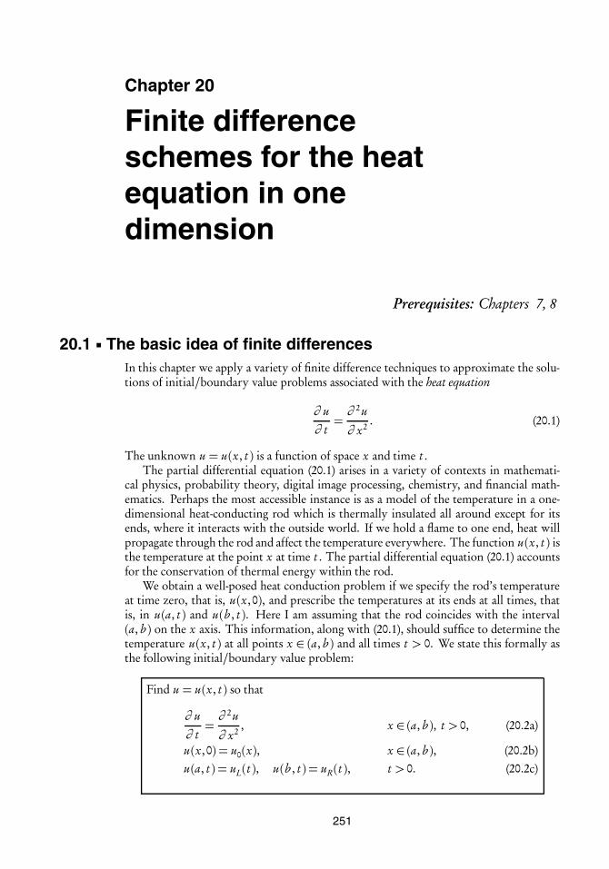
root2014/7/8page 251
�
�
�
�
�
�
�
�
Chapter 20
Finite differenceschemes for the heatequation in onedimension
Prerequisites: Chapters 7, 8
20.1 The basic idea of finite differencesIn this chapter we apply a variety of finite difference techniques to approximate the solu-tions of initial/boundary value problems associated with the heat equation
∂ u∂ t=∂ 2u
∂ x2 . (20.1)
The unknown u = u(x, t ) is a function of space x and time t .The partial differential equation (20.1) arises in a variety of contexts in mathemati-
cal physics, probability theory, digital image processing, chemistry, and financial math-ematics. Perhaps the most accessible instance is as a model of the temperature in a one-dimensional heat-conducting rod which is thermally insulated all around except for itsends, where it interacts with the outside world. If we hold a flame to one end, heat willpropagate through the rod and affect the temperature everywhere. The function u(x, t ) isthe temperature at the point x at time t . The partial differential equation (20.1) accountsfor the conservation of thermal energy within the rod.
We obtain a well-posed heat conduction problem if we specify the rod’s temperatureat time zero, that is, u(x, 0), and prescribe the temperatures at its ends at all times, thatis, in u(a, t ) and u(b , t ). Here I am assuming that the rod coincides with the interval(a, b ) on the x axis. This information, along with (20.1), should suffice to determine thetemperature u(x, t ) at all points x ∈ (a, b ) and all times t > 0. We state this formally asthe following initial/boundary value problem:
Find u = u(x, t ) so that
∂ u
∂ t=∂ 2u
∂ x2 , x ∈ (a, b ), t > 0, (20.2a)
u(x, 0) = u0(x), x ∈ (a, b ), (20.2b)u(a, t ) = uL(t ), u(b , t ) = uR(t ), t > 0. (20.2c)
251
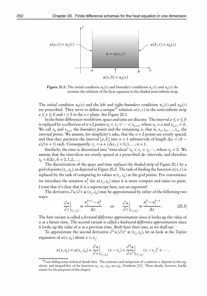
root2014/7/8page 252
�
�
�
�
�
�
�
�
252 Chapter 20. Finite difference schemes for the heat equation in one dimension
x
t
a b
u(a, t ) = uL(t ) u(b , t ) = uR(t )
u(x, 0) = u0(x)
u = u(x, t )
Figure 20.1: The initial condition u0(x) and boundary conditions uL(t ) and uR(t ) de-termine the solution of the heat equation in the shaded semi-infinite strip.
The initial condition u0(x) and the left and right boundary conditions uL(t ) and uR(t )are prescribed. They serve to define a unique79 solution u(x, t ) in the semi-infinite stripa ≤ x ≤ b and t > 0 in the x-t plane. See Figure 20.1.
In the finite differences worldview, space and time are discrete. The interval a ≤ x ≤ bis replaced by a collection of n+2 points x0 < x1 < · · ·< xn+1, where x0 = a and xn+1 = b .We call x0 and xn+1 the boundary points and the remaining n, that is, x1, x2, . . . , xn , theinternal points. We assume, for simplicity’s sake, that the n+ 2 points are evenly spaced,and thus they partition the interval [a, b ] into n + 1 subintervals of length Δx = (b −a)/(n+ 1) each. Consequently, xj = a+ jΔx, j = 0,1, . . . , n+ 1.
Similarly, the time is discretized into “time-slices” t0 < t1 < t2 · · · , where t0 = 0. Weassume that the time-slices are evenly spaced at a prescribed Δt intervals, and thereforetk = kΔt , k = 0,1,2, . . . .
The discretization of the space and time replaces the shaded strip of Figure 20.1 by agrid of points (xj , tk ), as depicted in Figure 20.2. The task of finding the function u(x, t ) isreplaced by the task of computing its values u(xj , tk ) at the grid points. For conveniencewe introduce the notation uk
j for u(xj , tk ) since it is more compact and easier to parse.I trust that it’s clear that k is a superscript here, not an exponent!
The derivative ∂ u/∂ t at (xj , tk )may be approximated by either of the following twoways:
∂ u
∂ t
����(xj ,tk )
≈ uk+1j − uk
j
Δtor
∂ u
∂ t
����(xj ,tk )
≈ ukj − uk−1
j
Δt. (20.3)
The first variant is called a forward difference approximation since it looks up the value ofu at a future time. The second variant is called a backward difference approximation sinceit looks up the value of u at a previous time. Both have their uses, as we shall see.
To approximate the second derivative ∂ 2u/∂ x2 at (xj , tk ), let us look at the Taylorexpansion of u(x, tk ) about x = xj :
u(x, tk ) = u(xj , tk )+∂ u
∂ x
����(xj ,tk )
(x − xj )+∂ 2u
∂ x2
����(xj ,tk )
(x − xj )2+ · · · .
79I am hiding some technical details here. The existence and uniqueness of a solution u depend on the reg-ularity and integrability of the functions u0, uL , uR; see e.g., Friedman [21]. Those details, however, hardlymatter for the purposes of this chapter.
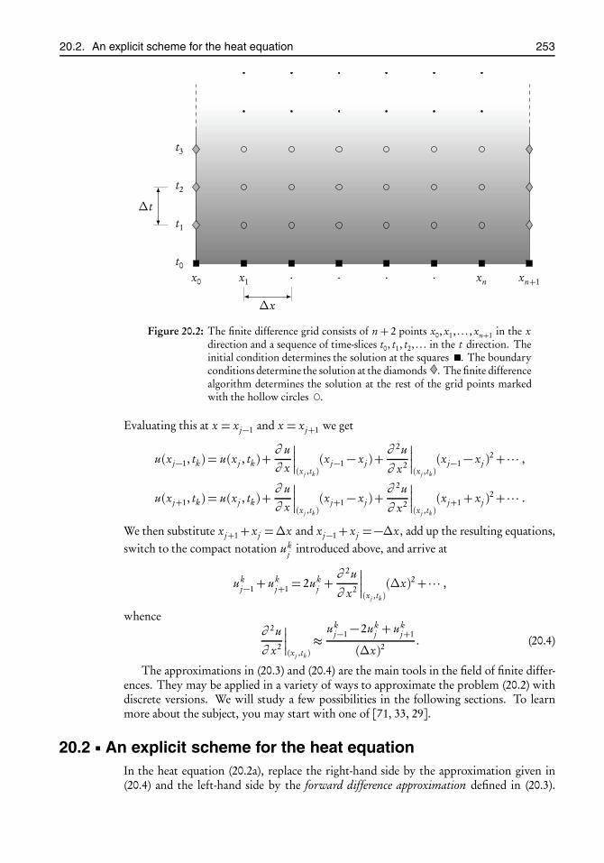
root2014/7/8page 253
�
�
�
�
�
�
�
�
20.2. An explicit scheme for the heat equation 253
x0 x1 · · · · xn xn+1
t0
t1
t2
t3
Δx
Δt
Figure 20.2: The finite difference grid consists of n + 2 points x0, x1, . . . , xn+1 in the xdirection and a sequence of time-slices t0, t1, t2, . . . in the t direction. Theinitial condition determines the solution at the squares . The boundaryconditions determine the solution at the diamonds . The finite differencealgorithm determines the solution at the rest of the grid points markedwith the hollow circles .
Evaluating this at x = xj−1 and x = xj+1 we get
u(xj−1, tk ) = u(xj , tk )+∂ u∂ x
����(xj ,tk )
(xj−1 − xj )+∂ 2u
∂ x2
����(xj ,tk )
(xj−1− xj )2+ · · · ,
u(xj+1, tk ) = u(xj , tk )+∂ u∂ x
����(xj ,tk )
(xj+1 − xj )+∂ 2u
∂ x2
����(xj ,tk )
(xj+1+ xj )2+ · · · .
We then substitute xj+1+ xj =Δx and xj−1+ xj =−Δx, add up the resulting equations,switch to the compact notation uk
j introduced above, and arrive at
ukj−1+ uk
j+1 = 2ukj +
∂ 2u
∂ x2
����(xj ,tk )
(Δx)2+ · · · ,
whence∂ 2u
∂ x2
����(xj ,tk )
≈ ukj−1− 2uk
j + ukj+1
(Δx)2. (20.4)
The approximations in (20.3) and (20.4) are the main tools in the field of finite differ-ences. They may be applied in a variety of ways to approximate the problem (20.2) withdiscrete versions. We will study a few possibilities in the following sections. To learnmore about the subject, you may start with one of [71, 33, 29].
20.2 An explicit scheme for the heat equationIn the heat equation (20.2a), replace the right-hand side by the approximation given in(20.4) and the left-hand side by the forward difference approximation defined in (20.3).
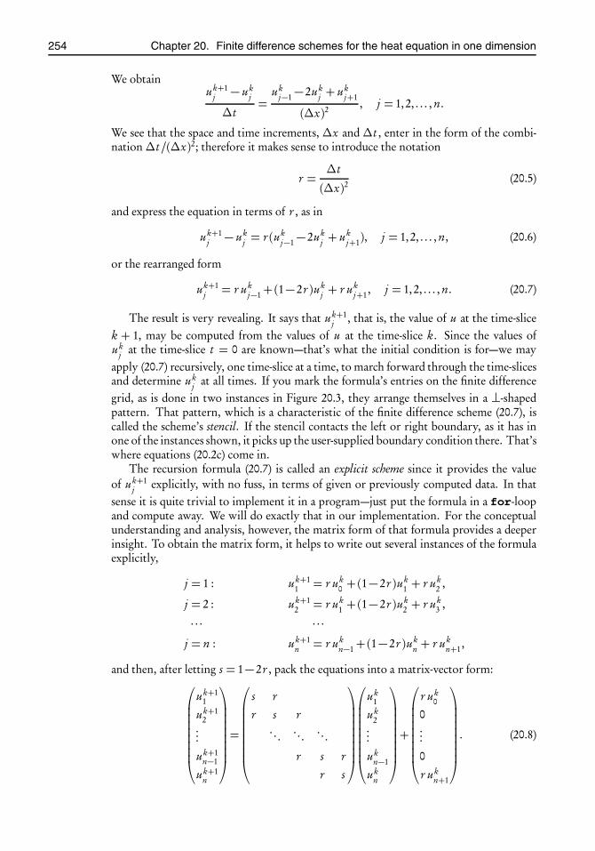
root2014/7/8page 254
�
�
�
�
�
�
�
�
254 Chapter 20. Finite difference schemes for the heat equation in one dimension
We obtainuk+1
j − ukj
Δt=
ukj−1− 2uk
j + ukj+1
(Δx)2, j = 1,2, . . . , n.
We see that the space and time increments, Δx and Δt , enter in the form of the combi-nationΔt/(Δx)2; therefore it makes sense to introduce the notation
r =Δt
(Δx)2(20.5)
and express the equation in terms of r , as in
uk+1j − uk
j = r (ukj−1− 2uk
j + ukj+1), j = 1,2, . . . , n, (20.6)
or the rearranged form
uk+1j = r uk
j−1+(1− 2r )ukj + r uk
j+1, j = 1,2, . . . , n. (20.7)
The result is very revealing. It says that uk+1j , that is, the value of u at the time-slice
k + 1, may be computed from the values of u at the time-slice k. Since the values ofuk
j at the time-slice t = 0 are known—that’s what the initial condition is for—we mayapply (20.7) recursively, one time-slice at a time, to march forward through the time-slicesand determine uk
j at all times. If you mark the formula’s entries on the finite differencegrid, as is done in two instances in Figure 20.3, they arrange themselves in a ⊥-shapedpattern. That pattern, which is a characteristic of the finite difference scheme (20.7), iscalled the scheme’s stencil. If the stencil contacts the left or right boundary, as it has inone of the instances shown, it picks up the user-supplied boundary condition there. That’swhere equations (20.2c) come in.
The recursion formula (20.7) is called an explicit scheme since it provides the valueof uk+1
j explicitly, with no fuss, in terms of given or previously computed data. In thatsense it is quite trivial to implement it in a program—just put the formula in a for-loopand compute away. We will do exactly that in our implementation. For the conceptualunderstanding and analysis, however, the matrix form of that formula provides a deeperinsight. To obtain the matrix form, it helps to write out several instances of the formulaexplicitly,
j = 1 : uk+11 = r uk
0 +(1− 2r )uk1 + r uk
2 ,
j = 2 : uk+12 = r uk
1 +(1− 2r )uk2 + r uk
3 ,
· · · · · ·j = n : uk+1
n = r ukn−1+(1− 2r )uk
n + r ukn+1,
and then, after letting s = 1− 2r , pack the equations into a matrix-vector form:⎛⎜⎜⎜⎜⎜⎜⎜⎜⎝
uk+11
uk+12
...
uk+1n−1
uk+1n
⎞⎟⎟⎟⎟⎟⎟⎟⎟⎠=
⎛⎜⎜⎜⎜⎜⎜⎜⎜⎝
s r
r s r. . . . . . . . .
r s r
r s
⎞⎟⎟⎟⎟⎟⎟⎟⎟⎠
⎛⎜⎜⎜⎜⎜⎜⎜⎜⎝
uk1
uk2
...
ukn−1
ukn
⎞⎟⎟⎟⎟⎟⎟⎟⎟⎠+
⎛⎜⎜⎜⎜⎜⎜⎜⎜⎝
r uk0
0...
0
r ukn+1
⎞⎟⎟⎟⎟⎟⎟⎟⎟⎠. (20.8)

root2014/7/8page 255
�
�
�
�
�
�
�
�
20.2. An explicit scheme for the heat equation 255
x0 x1 · · · · xn xn+1
t0
t1
t2
t3
Δx
Δt ukj−1 uk
j ukj+1
uk+1j
Figure 20.3: The explicit finite difference scheme acts on a ⊥-shaped stencil. It deter-mines the values of uk+1
j at the time-slice k+1 in terms of the three valuesof u from the previous time-slice. When the stencil hits the left or rightboundary, its picks up the prescribed boundary value from there.
The matrix is tridiagonal, having s = 1− 2r on its main diagonal and r on its first upperand lower subdiagonals. All other entries are zeros. We note that the matrix acts on thegrid’s internal nodes at the time-slice k. The additive vector in the equation’s extremeright imports the prescribed data from the boundary nodes x0 and xn+1. In effect, theequation defines a transition operator that maps the solution from the time-slice k to thetime-slice k + 1.
The recursion scheme (20.7), or its matrix equivalent (20.8), provides an extremelyquick and simple method for solving the heat equation and its relatives (general parabolicequations). Of course it is natural to ask the following: Does it produce a good approx-imation? Does the approximation improve as Δx and Δt go to zero? It turns out thatthe answers to both questions are a qualified “yes”. The catch is that you cannot takeΔxand Δt entirely independently of each other. The method is guaranteed to work only ifr ≤ 1/2, where r is defined in (20.5).
To get a feel for the source of the trouble, consider the special case where the boundaryconditions uL(t ) and uR(t ) in (20.2c) are zero. Then we expect the rod’s temperature togo to zero in the long run, regardless of the initial condition, since its ends are being keptat zero temperature. The finite difference scheme should confirm that. But does it?
When the boundary conditions are zero, the iteration scheme in (20.8) takes the formuk+1 =Auk , where A is the tridiagonal matrix in that equation, and uk is the vector thatit multiplies. We see that u1 = Au0, u2 =Au1, etc., and consequently uk = Aku0. It canbe shown (see [33], for instance) that the eigenvalues of A are
λ j = 1− 2r cosjπ
n+ 1, j = 1,2, . . . , n. (20.9)
Therefore, if r ≤ 1/2, then all eigenvalues are strictly less than 1, and consequently Ak → 0as k →∞, confirming our expectation. If r > 1/2, however, and n is sufficiently large,

root2014/7/8page 256
�
�
�
�
�
�
�
�
256 Chapter 20. Finite difference schemes for the heat equation in one dimension
then it is possible for some of the eigenvalues to be greater than 1; therefore Aku0 willgrow unbounded as k →∞, at least for some choices of u0. That is a totally unreasonableway for heat to behave; the iteration is producing junk!
An iteration scheme is said to be stable if small perturbations in the problem’s dataresult only in small perturbations in the solution. Otherwise it is said to be unstable. Theexplicit finite difference scheme defined by (20.7)—or the equivalent (20.8)—is condition-ally stable: it is stable when r ≤ 1/2.
Why should conditional stability concern us? Even with the most generous choiceof r = 1/2, (20.5) tells us that Δt = 1
2 (Δx)2. This implies that if Δx is small, then Δtwill be uncomfortably small. For instance, if Δx = 1/10, then Δt = 1/200. Thus, tocompute the solution up to time t = 1, we will have to march through 200 time-slices.If we change Δx to 1/100 to achieve a higher accuracy, then Δt changes to 1/20,000,forcing us to plod through 20,000(!) time-slices to traverse the time interval 0 to 1. That’san inordinate amount of work.
The implicit finite difference scheme, introduced in the next section, removes thatrestriction on r .
20.3 An implicit scheme for the heat equationIn the heat equation (20.2a), replace the right-hand side by the approximation given in(20.4) and the left-hand side by the backward difference approximation defined in (20.3).We obtain
ukj − uk−1
j
Δt=
ukj−1− 2uk
j + ukj+1
(Δx)2, j = 1,2, . . . , n.
For notational consistency with the previous section, shift the superscript k up by one,and also set r =Δt/(Δx)2, as before, to get
uk+1j − uk
j = r (uk+1j−1 − 2uk+1
j + uk+1j+1 ), j = 1,2, . . . , n. (20.10)
Then rearrange/group terms to arrive at
− r uk+1j−1 +(1+ 2r )uk+1
j − r u j+1j+1 = uk
j , j = 1,2, . . . , n. (20.11)
The formula’s entries form a�-shaped stencil on the finite difference grid. Two instancesof the stencil are shown in Figure 20.4. If the stencil contacts the left or right boundary,as it has in one of the instances shown, it picks up the user-supplied boundary conditionthere.
On the surface, this looks very similar to the previous section’s (20.7). There is, how-ever, something fundamentally different here. Equation (20.7) expresses u at the time-slicek + 1 explicitly in terms of the values of u at the previous time-slice. Equation (20.11),however, does not do that. It expresses a certain combination of the values of u at thetime-slice k + 1 in terms of u at the previous time-slice. It is called an implicit scheme forthat reason.
To grasp fully what the implicit scheme (20.11) represents, let us write it out in detail:
j = 1 : −r uk+10 +(1+ 2r )uk+1
1 − r uk+12 = uk
1 ,
j = 2 : −r uk+11 +(1+ 2r )uk+1
2 − r uk+13 = uk
2 ,
· · · · · ·j = n : −r uk+1
n−1+(1+ 2r )uk+1n − r uk+1
n+1 = ukn .

root2014/7/8page 257
�
�
�
�
�
�
�
�
20.3. An implicit scheme for the heat equation 257
x0 x1 · · · · xn xn+1
t0
t1
t2
t3
Δx
Δt
uk+1j−1 uk+1
j uk+1j+1
ukj
Figure 20.4: The implicit finite difference scheme acts on a�-shaped stencil. It relates alinear combination of three values of uk+1
j at the time-slice k+1 to a valueof u from the previous time-slice. When the stencil hits the left or rightboundary, its picks up the prescribed boundary value from there.
Then, after letting80 s = 1+ 2r , pack it into a matrix-vector form:⎛⎜⎜⎜⎜⎜⎜⎜⎜⎝
s −r
−r s −r. . . . . . . . .
−r s −r
−r s
⎞⎟⎟⎟⎟⎟⎟⎟⎟⎠
⎛⎜⎜⎜⎜⎜⎜⎜⎜⎝
uk+11
uk+12
...
uk+1n−1
uk+1n
⎞⎟⎟⎟⎟⎟⎟⎟⎟⎠=
⎛⎜⎜⎜⎜⎜⎜⎜⎜⎝
uk1
uk2
...
ukn−1
ukn
⎞⎟⎟⎟⎟⎟⎟⎟⎟⎠+
⎛⎜⎜⎜⎜⎜⎜⎜⎜⎝
r uk+10
0...
0
r uk+1n+1
⎞⎟⎟⎟⎟⎟⎟⎟⎟⎠. (20.12)
The matrix is tridiagonal, having s = 1+2r on its main diagonal and−r on its first upperand lower subdiagonals. All other entries are zeros. As a whole, the equation relates thestate of the solution at the grid’s internal nodes at the time-slice k+1 to those at the time-slice k. The additive vector in the equation’s extreme right imports the prescribed datafrom the boundary nodes x0 and xn+1.
Computing the solution at the time-slice k + 1 calls for solving the system of linearequations (20.12). The task is quite simple on account of the coefficient matrix beingtridiagonal. We will study the solution algorithm in subsection 20.9.3. For now, let uslook at the scheme’s stability.
As in the previous section, consider the special case where the boundary conditionsuL(t ) and uR(t ) in (20.2c) are zero. Then the iteration scheme in (20.12) takes the formBuk+1 = uk , where B is the tridiagonal matrix. We see that Bu1 = u0, Bu2 = u1, etc.,and consequently Bkuk = u0, and therefore uk = B−ku0.
Considering that s = 1+ 2r in this section while s = 1− 2r in the previous section,it should be evident that the matrix B here is related to the previous section’s matrixA through the change of variables r → −r . Therefore B’s eigenvalues are obtained by
80Beware that s = 1+ 2r is different from the previous definition of s .

root2014/7/8page 258
�
�
�
�
�
�
�
�
258 Chapter 20. Finite difference schemes for the heat equation in one dimension
changing r to−r in (20.9). Thus, B−1’s eigenvalues are
λ j =1
1+ 2r cos jπn+1
, j = 1,2, . . . , n.
We see that these are all strictly less than 1 regardless of the value of r (we are takingit for granted that r > 0). It follows that B−k → 0 as k → ∞; therefore the iterationscheme (20.12) is stable for all r . One expresses this by saying that the scheme is uncondi-tionally stable.
Unconditional stability is a good thing since it removes the worry about the rightchoice of r . But lest you jump to unwarranted conclusions, let me point out that thingsare not quite as rosy as you might expect.
Toward the end of the previous section, when discussing the stability of the explicitscheme, I noted that the requirement r ≤ 1/2 is quite inconvenient since Δt = r (Δx)2forces exceedingly small time-steps when Δx is somewhat small. The implicit scheme,however, imposes no restriction on r , so one may be tempted to take arbitrarily largetime-steps Δt , uncoupled from the size of Δx. This, however, does not work as well aswe may wish. It can be shown (see [33], for instance) that the discretization error in theimplicit scheme is of the order of magnitude of Δt + (Δx)2. For best results we want tokeep Δt and (Δx)2 in more or less comparable sizes; otherwise the larger of the two willdominate the error. This, in effect, limits Δt to something of the order of magnitude of(Δx)2 even though there is no restriction on r . The implicit scheme, therefore, has notreleased us from the bind of small time-steps.
The Crank–Nicolson scheme, introduced in the next section, gets around this dilemma.
20.4 The Crank–Nicolson scheme for the heat equationThe Crank–Nicolson scheme is obtained by summing the explicit and implicit differenc-ing formulas (20.6) and (20.10),
2(uk+1j − uk
j ) = r�uk
j−1 − 2ukj + uk
j+1 + uk+1j−1 − 2uk+1
j + uk+1j+1
,
and regrouping:
− r uk+1j−1 +2(1+ r )uk+1
j − r uk+1j+1 = r uk
j−1+2(1− r )ukj + r uk
j+1, j = 1,2, . . . , n. (20.13)
The formula’s entries form a -shaped stencil on the finite difference grid. Two instancesof the stencil are shown in Figure 20.5. If the stencil contacts the left or right boundary,as it has in one of the instances shown, it picks up the user-supplied boundary conditionsthere.
To fully grasp what the Crank–Nicolson scheme (20.13) represents, let us write it outin detail:
j = 1 : − r uk+10 + 2(1+ r )uk+1
1 − r uk+12 = r uk
0 + 2(1− r )uk1 + r uk
2 ,
j = 2 : − r uk+11 + 2(1+ r )uk+1
2 − r uk+13 = r uk
1 + 2(1− r )uk2 + r uk
3 ,
· · · · · ·j = n : − r uk+1
n−1 + 2(1+ r )uk+1n − r uk+1
n+1 = r ukn−1+ 2(1− r )uk
n + r ukn+1.

root2014/7/8page 259
�
�
�
�
�
�
�
�
20.4. The Crank–Nicolson scheme for the heat equation 259
x0 x1 · · · · xn xn+1
t0
t1
t2
t3
Δx
Δt ukj−1 uk
j ukj+1
uk+1j−1 uk+1
j uk+1j+1
Figure 20.5: The Crank–Nicolson finite difference scheme acts on an -shaped stencil.It relates a linear combination of three values of u k+1
j at the time-slice k+1to three values of u from the previous time-slice. When the stencil hits theleft or right boundary, its picks up the prescribed boundary values fromthere.
After setting81 s = 2(1+ r ) and s ′ = 2(1− r ), it takes the form
⎛⎜⎜⎜⎜⎜⎜⎜⎜⎝
s −r
−r s −r. . . . . . . . .
−r s −r
−r s
⎞⎟⎟⎟⎟⎟⎟⎟⎟⎠
⎛⎜⎜⎜⎜⎜⎜⎜⎜⎝
uk+11
uk+12
...
uk+1n−1
uk+1n
⎞⎟⎟⎟⎟⎟⎟⎟⎟⎠
=
⎛⎜⎜⎜⎜⎜⎜⎜⎜⎝
s ′ r
r s ′ r. . . . . . . . .
r s ′ r
r s ′
⎞⎟⎟⎟⎟⎟⎟⎟⎟⎠
⎛⎜⎜⎜⎜⎜⎜⎜⎜⎝
uk1
uk2
...
ukn−1
ukn
⎞⎟⎟⎟⎟⎟⎟⎟⎟⎠+
⎛⎜⎜⎜⎜⎜⎜⎜⎜⎝
r uk0 + r uk+1
0
0...
0
r ukn+1+ r uk+1
n+1
⎞⎟⎟⎟⎟⎟⎟⎟⎟⎠. (20.14)
It can be shown that the Crank–Nicolson scheme is unconditionally stable for all r >0. That’s good news. Even better news is that the discretization error of this scheme isof the order (Δt )2+ (Δx)2. Unlike the previous section’s implicit scheme, here Δt andΔx occur in equal powers. This allows taking time-steps of the same order of magnitudeas the space discretization. For this reason, Crank–Nicolson should be your default finitedifference scheme unless other considerations prevail.
81Beware that s = 2(1+ r ) is different from the previous definitions of s .
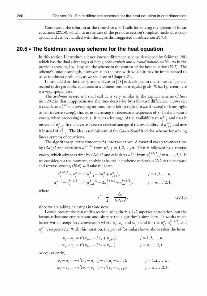
root2014/7/8page 260
�
�
�
�
�
�
�
�
260 Chapter 20. Finite difference schemes for the heat equation in one dimension
Computing the solution at the time-slice k + 1 calls for solving the system of linearequations (20.14), which, as in the case of the previous section’s implicit method, is tridi-agonal and can be handled with the algorithm suggested in subsection 20.9.3.
20.5 The Seidman sweep scheme for the heat equationIn this section I introduce a lesser known difference scheme developed by Seidman [58]which has the dual advantages of being both explicit and unconditionally stable. As in theprevious sections, I will explain the scheme in the context of the heat equation (20.2). Thescheme’s unique strength, however, is in the ease with which it may be implemented tosolve nonlinear problems, as we shall see in Chapter 21.
I must add that the theory and analysis in [58] is developed in the context of generalsecond order parabolic equations in n dimensions on irregular grids. What I present hereis a very special case.
The Seidman sweep, as I shall call it, is very similar to the explicit scheme of Sec-tion 20.2 in that it approximates the time derivative by a forward difference. However,it calculates uk+1
j in a sweeping motion, from left to right (forward sweep) or from rightto left (reverse sweep), that is, in increasing or decreasing sequences of j . In the forwardsweep, when processing node j , it takes advantage of the availability of uk+1
j−1 and uses it
instead of ukj−1. In the reverse sweep it takes advantage of the availability of uk+1
j+1 and uses
it instead of ukj−1. The idea is reminiscent of the Gauss–Seidel iterative scheme for solving
linear systems of equations.The algorithm splits the time-stepΔt into two halves. A forward sweep advances time
by (Δt )/2 and calculates uk+1/2j from uk
j , j = 1,2, . . . , n. That is followed by a reverse
sweep, which advances time by (Δt )/2 and calculates uk+1j from uk+1/2
j , j = n, . . . , 2,1. Ifwe consider, for the moment, applying the explicit scheme of Section 20.2 to the forwardand reverse sweeps, (20.6) will take the form
uk+1/2j − uk
j = r ′(ukj−1− 2uk
j + ukj+1), j = 1,2, . . . , n,
uk+1j − uk+1/2
j = r ′(uk+1/2j−1 − 2uk+1/2
j + uk+1/2j+1 ), j = n, . . . , 2,1,
where
r ′ =r2=
Δt
2(Δx)2, (20.15)
since we are taking half steps in time now.I could present the rest of this section using the k + 1/2 superscript notation, but the
formulas become cumbersome and obscure the algorithm’s simplicity. It works muchbetter with a temporary convention where uj , vj , and wj stand for the uk
j , uk+1/2j , and
uk+1j , respectively. With this notation, the pair of formulas shown above takes the form
vj − uj = r ′(uj−1− 2uj + uj+1), j = 1,2, . . . , n,
wj − vj = r ′(vj−1− 2vj + vj+1), j = n, . . . , 2,1,
or equivalently,
vj − uj =−r ′(uj − uj−1)− r ′(uj − uj+1), j = 1,2, . . . , n,
wj − vj =−r ′(vj − vj−1)− r ′(vj − vj+1), j = n, . . . , 2,1.
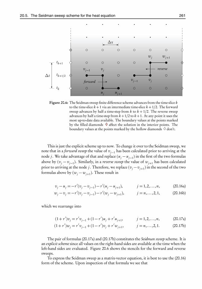
root2014/7/8page 261
�
�
�
�
�
�
�
�
20.5. The Seidman sweep scheme for the heat equation 261
tk
tk+1/2
tk+1
Δx
Δt
vj−1 vj
uj uj+1
forward vj−1 vj
wj wj+1
reverse
Figure 20.6: The Seidman sweep finite difference scheme advances from the time-slice kto the time-slice k+ 1 via an intermediate time-slice k+ 1/2. The forwardsweep advances by half a time-step from k to k + 1/2. The reverse sweepadvances by half a time-step from k+1/2 to k+1. At any point it uses themost up-to-date data available. The boundary values at the points markedby the filled diamonds affect the solution in the interior points. Theboundary values at the points marked by the hollow diamonds don’t.
This is just the explicit scheme up to now. To change it over to the Seidman sweep, wenote that in a forward sweep the value of vj−1 has been calculated prior to arriving at thenode j . We take advantage of that and replace (uj − uj−1) in the first of the two formulasabove by (vj − vj−1). Similarly, in a reverse sweep the value of wj+1 has been calculatedprior to arriving at the node j . Therefore, we replace (vj −vj+1) in the second of the twoformulas above by (wj −wj+1). These result in
vj − uj =−r ′(vj − vj−1)− r ′(uj − uj+1), j = 1,2, . . . , n, (20.16a)
wj − vj =−r ′(vj − vj−1)− r ′(wj −wj+1), j = n, . . . , 2,1, (20.16b)
which we rearrange into
(1+ r ′)vj = r ′vj−1 +(1− r ′)uj + r ′uj+1, j = 1,2, . . . , n, (20.17a)
(1+ r ′)wj = r ′vj−1 +(1− r ′)vj + r ′wj+1, j = n, . . . , 2,1. (20.17b)
The pair of formulas (20.17a) and (20.17b) constitutes the Seidman sweep scheme. It isan explicit scheme since all values on the right-hand sides are available at the time when theleft-hand sides are evaluated. Figure 20.6 shows the stencils for the forward and reversesweeps.
To express the Seidman sweep as a matrix-vector equation, it is best to use the (20.16)form of the scheme. Upon inspection of that formula we see that

root2014/7/8page 262
�
�
�
�
�
�
�
�
262 Chapter 20. Finite difference schemes for the heat equation in one dimension
⎛⎜⎜⎜⎜⎜⎝v1v2...vn−1vn
⎞⎟⎟⎟⎟⎟⎠−⎛⎜⎜⎜⎜⎜⎝
u1u2...un−1un
⎞⎟⎟⎟⎟⎟⎠=−r ′
⎛⎜⎜⎜⎜⎜⎝1 0
−1 1 0... .. . . . .
−1 1 0−1 1
⎞⎟⎟⎟⎟⎟⎠⎛⎜⎜⎜⎜⎜⎝
v1v2...vn−1vn
⎞⎟⎟⎟⎟⎟⎠
− r ′
⎛⎜⎜⎜⎜⎜⎝1 −10 1 −1
... .. . . . .0 1 −1
0 1
⎞⎟⎟⎟⎟⎟⎠⎛⎜⎜⎜⎜⎜⎝
u1u2...un−1un
⎞⎟⎟⎟⎟⎟⎠+ r ′
⎛⎜⎜⎜⎜⎜⎝v00...0un+1
⎞⎟⎟⎟⎟⎟⎠ .
Writing u, v, and w for the column vectors with the components uj , vj , wj and letting
A=
⎛⎜⎜⎜⎜⎜⎝1 0
−1 1 0... .. . . . .
−1 1 0−1 1
⎞⎟⎟⎟⎟⎟⎠ , a=
⎛⎜⎜⎜⎜⎜⎝v00...0un+1
⎞⎟⎟⎟⎟⎟⎠ , b=
⎛⎜⎜⎜⎜⎜⎝v00...0wn+1
⎞⎟⎟⎟⎟⎟⎠ ,
this takes on the compact form v−u=−r ′Av− r ′AT u+ r ′a, or equivalently,
(I + r ′A)v = (I − r ′AT )u+ r ′a, (20.18a)
where I is the identity matrix and AT is the transpose of A. Similar considerations regard-ing the reverse sweep in the formula (20.16b) lead to
(I + r ′AT )w = (I − r ′A)v+ r ′b. (20.18b)
The analysis in [58] shows that the iteration scheme expressed in the pair of equa-tions (20.18a) and (20.18b) is unconditionally stable for all r ′ > 0. I am not aware of astudy of the scheme’s rate of convergence, and I have not analyzed it myself. Numericalexperiments—see the error graphs in Figure 20.7—point to a rate of convergence of theorder (Δx)2+(Δt )2+ (Δt )2
(Δx)2, like that of the Du Fort–Frankel scheme (see [71]), but that’s
a mere conjecture on my part.
In favor of the Seidman sweep, one may note the following:
1. The Seidman sweep, being an explicit method, is easy to program, as we shall seelater in this chapter.
2. The Seidman sweep handles discontinuities in the initial and boundary conditionsmore gracefully than Crank–Nicolson.
3. The Seidman sweep has a definite advantage over implicit schemes in solving non-linear problems. An implicit scheme, such as Crank–Nicolson, requires solving ann × n nonlinear tridiagonal system at every step. The Seidman sweep, being anexplicit scheme, needs to solve 2n single (uncoupled) nonlinear equations in everyforward/reverse sweep pair. Chapter 21 applies the Seidman sweep to solve thehighly nonlinear porous medium equation.
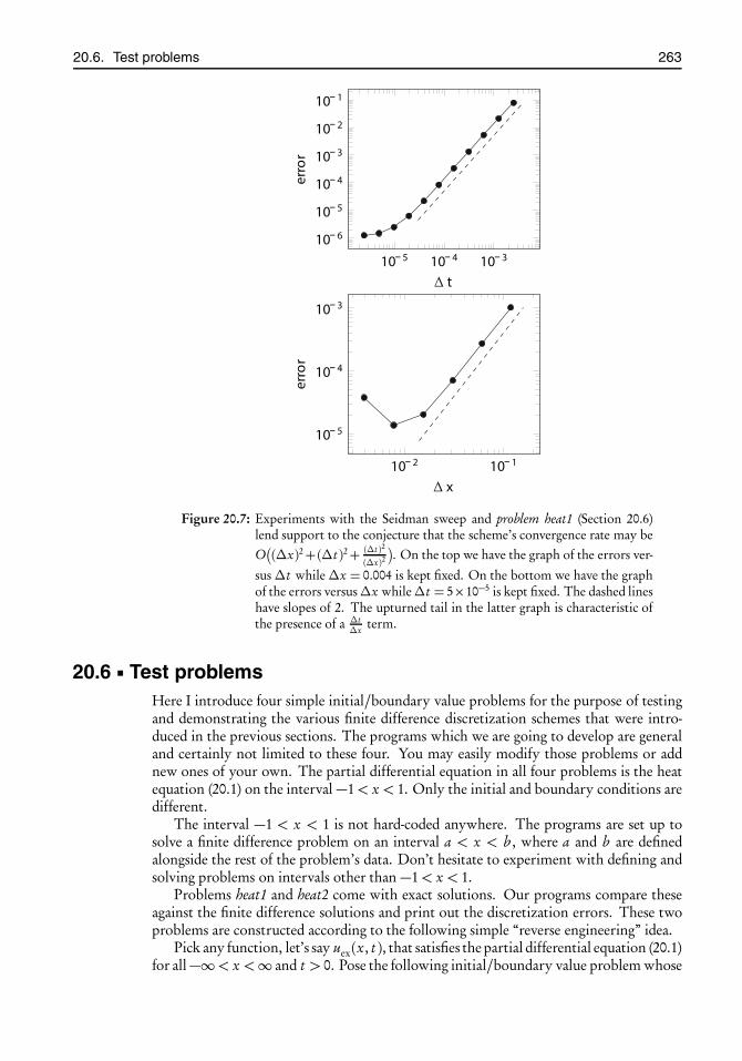
root2014/7/8page 263
�
�
�
�
�
�
�
�
20.6. Test problems 263
10 5 10 4 10 3
10 6
10 5
10 4
10 3
10 2
10 1
terror
10 2 10 1
10 5
10 4
10 3
x
error
Figure 20.7: Experiments with the Seidman sweep and problem heat1 (Section 20.6)lend support to the conjecture that the scheme’s convergence rate may beO�(Δx)2+(Δt )2+ (Δt )2
(Δx)2 . On the top we have the graph of the errors ver-
sus Δt while Δx = 0.004 is kept fixed. On the bottom we have the graphof the errors versusΔx whileΔt = 5×10⁻⁵ is kept fixed. The dashed lineshave slopes of 2. The upturned tail in the latter graph is characteristic ofthe presence of a Δt
Δx term.
20.6 Test problemsHere I introduce four simple initial/boundary value problems for the purpose of testingand demonstrating the various finite difference discretization schemes that were intro-duced in the previous sections. The programs which we are going to develop are generaland certainly not limited to these four. You may easily modify those problems or addnew ones of your own. The partial differential equation in all four problems is the heatequation (20.1) on the interval −1< x < 1. Only the initial and boundary conditions aredifferent.
The interval −1 < x < 1 is not hard-coded anywhere. The programs are set up tosolve a finite difference problem on an interval a < x < b , where a and b are definedalongside the rest of the problem’s data. Don’t hesitate to experiment with defining andsolving problems on intervals other than −1< x < 1.
Problems heat1 and heat2 come with exact solutions. Our programs compare theseagainst the finite difference solutions and print out the discretization errors. These twoproblems are constructed according to the following simple “reverse engineering” idea.
Pick any function, let’s say uex(x, t ), that satisfies the partial differential equation (20.1)for all−∞< x <∞ and t > 0. Pose the following initial/boundary value problem whose

root2014/7/8page 264
�
�
�
�
�
�
�
�
264 Chapter 20. Finite difference schemes for the heat equation in one dimension
data is defined in terms of uex(x, t ):⎧⎪⎪⎪⎪⎪⎪⎨⎪⎪⎪⎪⎪⎪⎩
∂ u
∂ t=∂ 2u
∂ x2 , x ∈ (a, b ), t > 0,
u(x, 0) = uex(x, 0), x ∈ (a, b ),u(a, t ) = uex(a, t ), t > 0,u(b , t ) = uex(b , t ), t > 0.
(20.19)
Clearly u(x, t ) = uex(x, t ) is a solution of the problem. (Actually, it’s the solution sincesuch problems have unique solutions.) To test the accuracy of our solvers, we have themsolve (20.19) and then compare the results with uex(x, t ).
Problem heat1: You should have no difficulty in verifying that the function
uex(x, t ) = e− 12π
2 t cos1
2πx (20.20)
is a solution of the heat equation (20.1). Check that for yourself! We define the problemheat1 by plugging (20.20) into the general template (20.19) with a =−1, b = 1.
Problem heat2: The error function, erf, despite its infelicitous appellation, occurs quitefrequently in the study of differential equations, probability, and statistics. It is defined as
erf(x) =2�π
∫ x
0e−t 2
d t .
The domain of erf is the entire real line. It increases monotonically from −1 at x =−∞to +1 at x =+∞. Figure 20.8 depicts its graph. Since the derivative of erf(x) is 2�
πe−x2
,you should be able to verify without much trouble that the function
uex(x, t ) = erf�
x
2�
t
�(20.21)
is an exact solution of the heat equation (20.1). We wish to use this finding to “reverse-engineer” an initial/boundary value problem according to the template (20.19), but we hita snag: The second of the equations in (20.1) calls for the value of uex(x, 0). Plugging t = 0in (20.21) won’t do since that would entail a division by zero on account of the
�t in the
denominator. We get around this by observing that although the expression uex(x, t ) isundefined at t = 0, its limit as t approaches zero from above does exist:
limt→0+
uex(x, t ) =�−1 if x < 0,+1 if x > 0.
This still leaves out the x = 0 case. There is no way around that since uex(x, t ) is ir-reparably discontinuous there. That’s not a significant obstacle, however, since the heatequation is good at smearing out discontinuities. Any value assigned to uex(0,0) will fadeaway quite fast. In our program we let uex(0,0) = 0. That’s as good a choice as any. Thus,our uex really looks like this:
uex(x, t ) =
⎧⎪⎪⎪⎪⎨⎪⎪⎪⎪⎩erf
*x
2�
t
+if t > 0,
−1 if t = 0 and x < 0,+1 if t = 0 and x > 0,0 if t = 0 and x = 0.
(20.22)

root2014/7/8page 265
�
�
�
�
�
�
�
�
20.6. Test problems 265
−4 −2 2 4
−1
−0.5
0.5
1
x
erf(x)
Figure 20.8: The graph of the error function erf(x).
With the continuity issue out of the way, we define the problem heat2 by plugging (20.22)into the general template (20.19) with a =−1, b = 1.
Remark 20.1. Due to the linearity of the heat equation (20.1), any constant multiple ofa solution is also a solution. In the implementation of problem heat2, I use 0.4× uex(x, t )since the resulting flattened graph has a more appealing look. There is no deep reasonbehind that choice.
Problem heat3: Take the “rectangular bump” function
u0(x) =�
1, |x|< 0.4,0 otherwise
for the initial condition, and define the problem heat3 as⎧⎪⎪⎪⎨⎪⎪⎪⎩∂ u
∂ t=∂ 2u
∂ x2 , x ∈ (−1,1), t > 0,
u(x, 0) = u0(x), x ∈ (−1,1),u(−1, t ) = u(1, t ) = 0, t > 0.
Problem heat4: This problem is defined as⎧⎪⎪⎪⎪⎪⎪⎨⎪⎪⎪⎪⎪⎪⎩
∂ u∂ t=∂ 2u
∂ x2 , x ∈ (−1,1), t > 0,
u(x, 0) = 0, x ∈ (−1,1),u(−1, t ) = 0, t > 0,u(1, t ) = 0.8, t > 0.
What does this say about the value of the solution at x = 1, t = 0?. The initial conditionsays u(1,0) is 0. The boundary condition says u(1,0) is 0.8. Therefore we expect thesolution u(x, t ) to be discontinuous at x = 0, t = 0. The purpose of this problem is toexamine how well the various finite difference schemes handle that discontinuity.

root2014/7/8page 266
�
�
�
�
�
�
�
�
266 Chapter 20. Finite difference schemes for the heat equation in one dimension
20.7 The programThe rest of this chapter is devoted to details of the implementations of the four finitedifference schemes introduced in the previous sections. We will write four individualprograms, one for each scheme, encoded in the files heat-explicit.c, heat-implicit.c, heat-crank-nicolson.c, and heat-seidman-sweep.c. The problems to be solved are defined in afile named problem-spec.c, which may contain any number of initial/boundary valueproblems.
We rely on xmalloc.[ch] from Chapter 7 to allocate memory and the file array.h fromChapter 8 to construct vectors and matrices. Thus, following the suggestions in Chap-ters 2 and 6, the contents of the project’s directory will look like this:
$ cd fd1$ ls -FMakefile heat-implicit.c [email protected]@ heat-seidman-sweep.c [email protected] problem-spec.cheat-explicit.c problem-spec.h
I have named my directoryfd1 since the programs here deal with finite difference schemesin a one-dimensional space.
There is a good deal of duplication among the heat-*.c files since the supporting code—parsing the command-line arguments, computing errors, plotting the solutions—is com-mon to all four. It is possible to merge the four programs into one and factor out thecommon parts, but the logic can get a bit twisty; therefore I will not go down that path.You are welcome to try it if you wish.
Currently my problem-spec.c contains four boundary value problems named heat1,heat2, heat3, heat4 that were introduced in the previous section. Each of these can besolved with any of the four finite difference schemes; therefore we are going to produce atotal of 16 solutions altogether.
Conceptually, each solution is a matrix of the computed ukj values of the solution at
the finite difference grid points. We may set up the programs to print out those matricesas tables of numbers, but it is more informative to produce pictures of the graphs of thesolutions u(x, t ) as surfaces drawn in three dimensions. Thus, for each solution we writethe grid values to a file in a special format that is suitable for feeding to Geomview (seepage 8) which will render the surface on your computer screen and let you rotate it withthe mouse. The graphs of the various solutions shown in this chapter are snapshots of aGeomview window.
Here is a transcript of a sample session with the heat-explicit program that implementsthe explicit scheme:
$ ./heat-explicitUsage: ./heat-explicit T n s
T : solve over 0 ≤ t ≤ Tn : number of grid points a=x[0], x[1], ... , x[n], x[n+1]=bs : number of time-slices 0=t[0], t[1], ... , t[s]=T
$ ./heat-explicit 0.2 9 10problem heat1:-1 < x < 1, 0 < t < 0.2, dx = 0.2, dt = 0.02, r = dt/dx^2 = 0.5geomview script written to file ex1.gvmax error at time 0.2 is 0.00506898

root2014/7/8page 267
�
�
�
�
�
�
�
�
20.8. The files problem-spec.[ch] 267
problem heat2:-1 < x < 1, 0 < t < 0.2, dx = 0.2, dt = 0.02, r = dt/dx^2 = 0.5geomview script written to file ex2.gvmax error at time 0.2 is 0.00999372
problem heat3:-1 < x < 1, 0 < t < 0.2, dx = 0.2, dt = 0.02, r = dt/dx^2 = 0.5geomview script written to file ex3.gv
problem heat4:-1 < x < 1, 0 < t < 0.2, dx = 0.2, dt = 0.02, r = dt/dx^2 = 0.5geomview script written to file ex4.gv
The meanings of the program’s arguments should be clear from the “Usage” message thatappears above. The programs heat-implicit, heat-crank-nicolson.c, and heat-seidman-sweep.cmay be invoked in the same way. Figures 20.9 and 20.10 shows the results of running thefour programs, each solving the four problems heat1, heat2, heat3, and heat4. The figures’captions give the command-line arguments with which the programs were invoked.
Since the problems heat1 and heat2 are supplied with exact solutions, the programcomputes and prints the error in those two cases. The error is defined by
err= max0≤ j≤n+1
|uex(xj ,T )− u sj |, (20.23)
where the superscript s corresponds to the time index at the time T , that is, ts = T .Let us note that heat-explicit was involved with the command-line arguments, 0.5 10 32.
In words, the problem is solved over the range 0≤ t ≤ 0.5 through 32 time-steps; thereforeΔt = 0.5/32= 1/64. The x domain, which is the interval (−1,1), has 10 internal nodes;therefore Δx = 2/11. We see that r = (Δt )/(Δx)2 ≈ 0.472656< 0.5, that is, the schemeis within the threshold of stability; see Section 20.2. In contrast, if we run heat-explicitwith the arguments 0.352 20 20, we will have r = 1.9404> 0.5; therefore the scheme willbe unstable. Figure 20.11 shows the resulting calamity when it’s applied to the problemheat1.
20.8 The files problem-spec.[ch]The file problem-spec.h provides a data structure designed to hold the definition of aninitial/boundary value problem. The file problem-spec.c uses that data structure to de-fine concrete realizations of any number of such problems. The next two subsectionsgive the details of the contents of these files.
20.8.1 The file problem-spec.h
The file problem-spec.h, shown in it entirety in Listing 20.1, declares a data structure named“struct problem_spec” for storing definitions of initial/boundary value problemsof the type (20.2) on page 251. The members a andb of that structure hold the coordinatesof the endpoints of the interval a ≤ x ≤ b . The member ic points to a function thatsupplies the problem’s initial condition u0(x), while the members bcL and bcR point tofunctions uL(t ) and uR(t ) that supply the left and right boundary conditions. Finally, themember u_exact points to a function that returns the problem’s exact solution. If sucha function is provided, the program will use it to compute and print the error (at the finaltime) in the finite difference scheme. If an exact solution is not available, set that pointerto NULL.
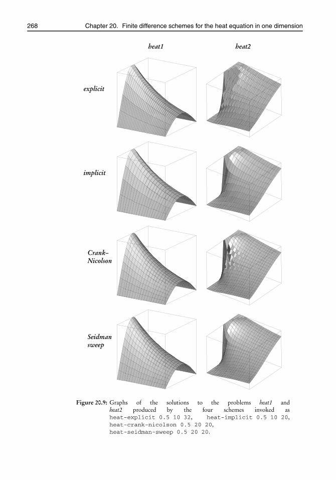
root2014/7/8page 268
�
�
�
�
�
�
�
�
268 Chapter 20. Finite difference schemes for the heat equation in one dimension
heat1 heat2
explicit
implicit
Crank–Nicolson
Seidmansweep
Figure 20.9: Graphs of the solutions to the problems heat1 andheat2 produced by the four schemes invoked asheat-explicit 0.5 10 32, heat-implicit 0.5 10 20,heat-crank-nicolson 0.5 20 20,heat-seidman-sweep 0.5 20 20.

root2014/7/8page 269
�
�
�
�
�
�
�
�
20.8. The files problem-spec.[ch] 269
heat3 heat4
explicit
implicit
Crank–Nicolson
Seidmansweep
Figure 20.10: Graphs of the solutions to the problems heat3 andheat4 produced by the four schemes invoked asheat-explicit 0.5 10 32, heat-implicit 0.5 10 20,heat-crank-nicolson 0.5 20 20,heat-seidman-sweep 0.5 20 20.

root2014/7/8page 270
�
�
�
�
�
�
�
�
270 Chapter 20. Finite difference schemes for the heat equation in one dimension
xt
u(x, t )
Figure 20.11: Running heat-explicit with the command-line arguments 0.352 20 20yields an unstable scheme since r = (Δt )/(Δx)2 ≈ 1.9404> 0.5. Here wesee the solution of the problem heat1 begin to fall apart as we approacht = 0.352. Beyond this the oscillations grow very large so quickly thatdrawing a graph is impractical.
Listing 20.1: The contents of the file problem-spec.h.
1 #ifndef H_PROBLEM_SPEC_H2 #define H_PROBLEM_SPEC_H3 struct problem_spec {4 double a; // left end at x = a5 double b; // right end at x= b6 double (*ic)(double x); // initial condition7 double (*bcL)(double t); // left boundary condition8 double (*bcR)(double t); // right boundary condition9 double (*u_exact)(double x, double t); // exact solution, if any
10 };11 #endif /∗ H_PROBLEM_SPEC_H */
20.8.2 The file problem-spec.c
My problem-spec.c contains the definitions of the four initial/boundary value problemsheat1, heat2, heat3, and heat4 introduced in Section 20.6. You are invited to modify theseor add problems of your own.
Listing 20.2 shows the part of the file problem-spec.c where the problem named heat1is defined. Following the “reverse-engineering” idea expounded in (20.19), I use the exactsolution given in (20.20) to set the problem’s initial and boundary conditions. Lines 6through 22 are self-explanatory, so there is no need to elaborate other than note that thecosine function, cos(), and the exponential function, exp(), are defined in C’s standardmathematics library; therefore you may need to link it to your program by specifying the-lm flag at the linking stage. The header file math.h (line 2) provides the prototypes ofthose functions.
Lines 23 through 35 define a function named heat1() that sets up and populatesa struct problem_spec with the problem’s data and returns the structure’s address.The static specifier on line 25 is absolutely essential. A static object is available

root2014/7/8page 271
�
�
�
�
�
�
�
�
20.8. The files problem-spec.[ch] 271
Listing 20.2: This is the top of my file problem-spec.c. It shows the requisite #includes, plus allthe components that define the problem heat1. I use the exact solution given in (20.20)to set the problem’s initial and boundary conditions.
1 #include <stdio.h>2 #include <math.h>3 #include "problem-spec.h"4
5 // heat1( ): quite a basic one-dimensional heat equation with exact solution6 static double heat1_exact(double x, double t)7 {8 double Pi = 4*atan(1);9 return exp(-Pi*Pi/4*t) * cos(Pi/2*x);
10 }11 static double heat1_ic(double x)12 {13 return heat1_exact(x,0);14 }15 static double heat1_bcL(double t)16 {17 return heat1_exact(-1,t);18 }19 static double heat1_bcR(double t)20 {21 return heat1_exact(1,t);22 }23 struct problem_spec *heat1(void)24 {25 static struct problem_spec spec = { // C99-style initialization!26 .a = -1.0,27 .b = 1.0,28 .ic = heat1_ic,29 .bcL = heat1_bcL,30 .bcR = heat1_bcR,31 .u_exact = heat1_exact,32 };33 printf("problem heat1:\n");34 return &spec;35 }
throughout the duration of the program’s execution. Without the static specifier, thestructure will come into existence when the function is entered and will evaporate whenthe function is exited. In that case returning the structure’s address would make no senseat all since it would be the address of an evaporated entity.82
I am initializing the structure à la C99. The program won’t compile if your compilerdoes not recognize the C99 syntax. See the comments under the Initializing structuresheading on page 6 if you wish to change the initialization to the equivalent C89 syntax.
82Listing 20.2 exhibits two completely unrelated meanings of C’s static keyword which should not beconfused. The one on line 25 pertains to the corresponding object’s lifetime, as explained above. All otheroccurrences of static in that listing pertain to linkage. The one on line 6, for instance, indicates that thefunction heat1_exact() is inaccessible/invisible outside this file. Consult your C reference/manual for amore detailed explanation.

root2014/7/8page 272
�
�
�
�
�
�
�
�
272 Chapter 20. Finite difference schemes for the heat equation in one dimension
Listing 20.3: An outline of the file heat-implicit.c.
1 � #include ...2 � static void trisolve(int n, double *a, double *d, double *c, double *b,3 double *x) ...4 � static double get_error(struct problem_spec *spec,5 double *u, int n, double T) ...6 � static void plot_curve(FILE *fp, double *u, int n, int steps, int k) ...7 � static void heat_implicit(struct problem_spec *spec,8 double T, int n, int steps, char *gv_filename) ...9 � static void show_usage(char *progname) ...
10 � int main(int argc, char **argv) ...
The problem heat2 is defined in the same way. We use the exact solution (20.22) to setthe problem’s initial and boundary conditions. I will leave it to you to supply the details.You will need to know that the error function, erf, is defined in C’s standard mathematicslibrary and is called erf().
Problems heat3 and heat4 do not come with predefined exact solutions; therefore wedefine their initial and boundary conditions from scratch. For example,
1 static double heat3_ic(double x)2 {3 return fabs(x) < 0.4 ? 1.0 : 0.0;4 }
Again, I will leave it to you to supply the remaining details.
20.9 The file heat-implicit.cIn this section I will go through the complete contents of the file heat-implicit.c, whichprovides an implementation of the implicit finite difference scheme for solving the heatequation. I will leave the writing of the files heat-explicit.c, heat-crank-nicolson.c, and heat-seidman-sweep.c as projects for you.
Listing 20.3 provides an outline of heat-implicit.c. The function main() parses thecommand-line arguments and then makes a sequence of calls, one per problem to besolved, to heat_implicit(), which, in turn, sets up a for-loop to march forwardthrough the time steps and at each step calls trisolve() to solve the tridiagonal sys-tem (20.12) and plot_curve() to construct a section of the three-dimensional surfaceplots that we see in Figures 20.9 and 20.10. Upon exiting the loop, if an exact solution isprovided, the function get_error() is called to print the discrepancy between the ex-act and computed solutions. The details of these functions are described in the subsectionsbelow, albeit not in the order that they appear in Listing 20.3.
20.9.1 The function main()
As we saw in the transcript of the interactive session with the program on page 266, theprogram is expected to be invoked with three arguments, as in
$ ./heat-implicit T n s
where T specifies the upper end of the time range 0 ≤ t ≤ T , n is the number of theinternal grid points in the x direction, and s is the number of time-steps. To be precise,

root2014/7/8page 273
�
�
�
�
�
�
�
�
20.9. The file heat-implicit.c 273
Listing 20.4: The function main() in the file heat-implicit.c. Lines 3–6 supply the prototypes ofthe functions heat1() through heat4(), which are defined in problem-spec.c.
1 int main(int argc, char **argv)2 {3 struct problem_spec *heat1(void);4 struct problem_spec *heat2(void);5 struct problem_spec *heat3(void);6 struct problem_spec *heat4(void);7 char *endptr;8 double T;9 int n, steps;
10 if (argc �= 4) {11 show_usage(argv[0]);12 return EXIT_FAILURE;13 }14 T = strtod(argv[1], &endptr);15 if (*endptr �= ’\0’ || T ≤ 0.0) {16 show_usage(argv[0]);17 return EXIT_FAILURE;18 }19 n = strtol(argv[2], &endptr, 10);20 if (*endptr �= ’\0’ || n < 1) {21 show_usage(argv[0]);22 return EXIT_FAILURE;23 }24 steps = strtol(argv[3], &endptr, 10);25 if (*endptr �= ’\0’ || steps < 0) {26 show_usage(argv[0]);27 return EXIT_FAILURE;28 }29 heat_implicit(heat1(), T, n, steps, "im1.gv");30 heat_implicit(heat2(), T, n, steps, "im2.gv");31 heat_implicit(heat3(), T, n, steps, "im3.gv");32 heat_implicit(heat4(), T, n, steps, "im4.gv");33 return EXIT_SUCCESS;34 }
the x coordinates of the grid points are a = x0, x1, . . . , xn , xn+1 = b , and the time-slicestake place at 0= t0, t1, . . . , ts = T . Therefore Δt = T /s andΔx = (b − a)/(n+ 1).
One of the tasks of the function main() that appears on line 10 of Listing 20.3 is toextract the values of T, n, and s from the command-line. Listing 20.4 gives the details ofits implementations.
Lines 3–6 supply the prototypes of the functions heat1() through heat4(), whichare defined in problem-spec.c. I could have put those prototypes in the file problem-spec.hbut chose not to since I don’t like the idea of a problem-spec.h file which changes withthe addition of every new problem in problem-spec.c. I have placed those prototypes inmain() since that’s the only place where they are needed.
Lines 10–28 extract the values of T , n, and s (the last is called steps in the code) fromthe command-line. See Chapter 5 regarding the functions strtod() and strtol().The next four lines call the function heat_implicit() four times to solve the fourproblems heat1, heat2, heat3, and heat4. The arguments heat1(), heat2(), heat3(),

root2014/7/8page 274
�
�
�
�
�
�
�
�
274 Chapter 20. Finite difference schemes for the heat equation in one dimension
and heat4() retrieve the “struct problem_spec” for each of the four problemsdefined in problem-spec.c. The arguments "im1.gv", etc., are file names to which theprogram is to write the computed solutions in the form of Geomview scripts for plotting.The file names are arbitrary, but it’s a good idea to name them so that they are easy for youto identify. When solving the problems with the Crank–Nicolson method, for instance,I would name them "cn1.gv", etc.
20.9.2 The function show_usage()
The function show_usage() that appears on line 9 of Listing 20.3 is responsible forprinting the “Usage” message shown in the transcript of the interactive session on page 266.It is called in several places in Listing 20.4. Implement the function, and add it to yourheat-implicit.c.
20.9.3 The function trisolve()
The function trisolve() that appears on line 2 of Listing 20.3 is a generic solver ofn× n tridiagonal linear systems of equations of the form
⎛⎜⎜⎜⎜⎜⎜⎜⎝
d0 c0a0 d1 c1
a1 d2 c2... . . . . . .
an−3 dn−2 cn−2an−2 dn−1
⎞⎟⎟⎟⎟⎟⎟⎟⎠
⎛⎜⎜⎜⎜⎜⎜⎜⎝
x0x1x2...xn−2xn−1
⎞⎟⎟⎟⎟⎟⎟⎟⎠=⎛⎜⎜⎜⎜⎜⎜⎜⎝
b0b1b2...bn−2bn−1
⎞⎟⎟⎟⎟⎟⎟⎟⎠ .
There is no point in storing the full n × n coefficient matrix. We store only the diag-onal ⟨d0, . . . , dn−1⟩, the subdiagonal ⟨a0, . . . ,an−2⟩, and the superdiagonal ⟨c0, . . . , cn−2⟩ asordinary vectors.
We assume that the coefficient matrix is nonsingular. Our code does not check forthat. It can be shown that matrices that arise through finite difference schemes applied toparabolic problems are nonsingular.
We solve the system through a simple Gaussian elimination without pivoting. Toeliminate a0, we introduce the multiplier m = a0/d0 and then subtract m times the firstequation from the second equation. This (i) reduces the entry in the a0 position to zero;(ii) changes the entry in the d1 position to d1−mc0; and (iii) changes the entry in the b1position to b1−mb0. The entry in the c1 position does not change.
We repeat the procedure to eliminate the rest of the subdiagonal, in sequence, fromtop to bottom. When operating on row i (i = 1,2, . . . , n − 1) we set m = ai−1/di−1 andthen subtract m times row i−1 from row i . This (i) eliminates the ai−1 entry; (ii) changesthe di entry to di −mci−1; and (iii) changes the bi entry to bi −mbi−1.
Listing 20.5 shows my implementation of trisolve(). In lines 4–8 you will findthe literal encoding of the statements made above.
Remark 20.2. We don’t bother to zero the ai entries in our code since we have no usefor the ai ’s beyond this point. Consequently, the elimination’s overall effect is to changethe di and bi vectors, but the ai and ci vectors remain unchanged! We take advantage ofthis when calling trisolve(), as we will see shortly.

root2014/7/8page 275
�
�
�
�
�
�
�
�
20.9. The file heat-implicit.c 275
Listing 20.5: The function trisolve() in the file heat-implicit.c.
1 static void trisolve(int n, double *a, double *d, double *c, double *b,2 double *x)3 {4 for (int i = 1; i < n; i++) {5 double m = a[i-1]/d[i-1];6 d[i] -= m*c[i-1];7 b[i] -= m*b[i-1];8 }9 x[n-1] = b[n-1]/d[n-1];
10 for (int i = n-2; i ≥ 0; i--)11 x[i] = (b[i] - c[i]*x[i+1]) / d[i];12 }
After eliminating the subdiagonal, the system takes the form⎛⎜⎜⎜⎜⎜⎜⎜⎝
d0 c0d1 c1
d2 c2... . . .
dn−2 cn−2dn−1
⎞⎟⎟⎟⎟⎟⎟⎟⎠
⎛⎜⎜⎜⎜⎜⎜⎜⎝
x0x1x2...xn−2xn−1
⎞⎟⎟⎟⎟⎟⎟⎟⎠=⎛⎜⎜⎜⎜⎜⎜⎜⎝
b0b1b2...bn−2bn−1
⎞⎟⎟⎟⎟⎟⎟⎟⎠ .
The di ’s and bi ’s are different from what they were before, but the ci ’s are the same. Thesystem’s last equation, that is, dn−1 xn−1 = bn−1, yields xn−1 = bn−1/dn−1. We computethe rest of the xi ’s through back substitution. To wit, the equation before the last, thatis, dn−2 xn−2 + cn−2xn−1 = bn−2, yields the value of xn−2 since xn−1 is already known.In general, the equation in row i (i = n − 2, . . . , 0), that is, di xi + ci xi+1 = bi , yieldsxi = (bi− ci xi+1)/di in terms of the previously calculated xi+1. Lines 9–11 in Listing 20.5reflect this finding.
20.9.4 The function plot_curve()
The function plot_curve() that appears on line 6 of Listing 20.3 is responsible forproducing the graphs shown in Figures 20.9 and 20.10 on pages 268 and 269. Well, to bepedantic, plot_curve() does not literally produce those graphs, Geomview does. Whatplot_curve() does is to help write a script which when fed to Geomview producesthose graphs.
To understand the details, we need to know what Geomview expects to see in its inputscript. The requirement is quite simple—to plot the graph of a function z = f (x, y) overan m× n mesh, we supply the graph’s (x, y, z) coordinates at the mesh points, where themesh is scanned from left to right in each row and then by rows from top to bottom. Wewrap the resulting sequence of N = mn coordinate triplets (x, y, z) in a minimal code tomake it palatable to Geomview and save it to a file, like this:
# the skeleton of a Geomview input file{ appearance { +edge }MESH m nx[1] y[1] z[1]x[2] y[2] z[2]

root2014/7/8page 276
�
�
�
�
�
�
�
�
276 Chapter 20. Finite difference schemes for the heat equation in one dimension
...x[N] y[N] z[N]}
The numbers are separated by whitespace.83 One or more consecutive whitespace countas one whitespace. Line breaks are not required; you may put the 3N numbers all on asingle line if you like. The “appearance { +edge }” at the top of the script tellsGeomview to draw the mesh lines. If you change +edge to -edge, the surface will bedrawn without the mesh lines. The keyword “MESH” should be typed in capital letters,as shown.
This is exactly how the graphs in Figures 20.9 and 20.10 were produced. Each graphdepicts the solution uk
j on an (n+2)× (s+1) grid, where n+2 and s+1 are the numbersof grid points in the x and t directions, respectively. As we will see in the next subsection,the values of uk
j are computed iteratively, one time-slice at a time, as vectors
u= ⟨uk0 , uk
1 , . . . , ukn , uk
n+1⟩ (20.24)
of length n + 2. The function plot_curve() receives the vector u. It calculates thecoordinates xj of the entry uk
j and appends the n+2 triplets (xj , tk , ukj ) to the Geomview
script. Sinceplot_curve() handles only one time-slice of the overall graph, it is named“plot curve” rather than “plot surface”.
Calculating the coordinates xj is straightforward. The finite difference scheme has ninternal grid points in the x direction; therefore the interval a ≤ x ≤ b is divided inton + 1 subintervals of length (b − a)/(n+ 1) each. It follows that the j th grid point is atxj = a+
�(b − a)/(n+ 1)
�j , j = 0,1, . . . , n+ 1. Similarly, since we are taking s steps over
the time interval 0≤ t ≤ T , then tk = T k/s , k = 0,1, . . . , s .A direct implementation of the calculation above, however, can produce disappoint-
ing results. Here is why.Suppose we solve an initial/boundary value problem over the domain D = {(x, t ) :
−1≤ x ≤ 1, 0≤ t ≤ 0.1}, which is a 2×0.1 rectangle. Plotting the solution to the correctscale over this long and narrow rectangle will produce a pretty useless graph. Since it’s sonarrow, one won’t be able to see any details.
It is preferable to forgo the correct scaling in favor of stretching D into a square forplotting purposes. That’s quite a natural thing to do, and that is what I have done in allthe graphs shown in this chapter. Had you noticed that before I mentioned it?
So here is the idea: Instead of using the true xj coordinates calculated above, just usexj = j/(n+1), j = 0,1, . . . , n+1. As j ranges from 0 to n+1, the values of xj range from0 to 1. Similarly, instead of using the true tk values calculated above, just take tk = k/s .As k ranges from 0 to s , the values of tk range from 0 to 1. The net result is that thedomain D is replaced by the square [0,1]× [0,1] for plotting purposes.
Remark 20.3. The natural next step is to scale and translate the u values to the range[0,1] so that the displayed graph lies entirely within the cube [0,1]× [0,1]× [0,1]. I willdefer this to a (not so difficult) project in this chapter’s Projects section. I have posed theproblems heat1 through heat4 so that their u values lie more or less in the [0,1] range toobviate a need for scaling. To view the solutions to arbitrary problems you will definitelyneed to scale.
83It’s safe if you think of “whitespace” as the characters produced by the keyboard’s space-bar or tab or enterkeys. For the precise meaning of “whitespace” see subsection 9.3.2.

root2014/7/8page 277
�
�
�
�
�
�
�
�
20.9. The file heat-implicit.c 277
Listing 20.6: The implementation of the function plot_curve() in the file heat-implicit.c.
1 static void plot_curve(FILE *fp, double *u, int n, int steps, int k)2 {3 for (int j = 0; j < n+2; j++)4 fprintf(fp, "%g %g %g\n",5 (double)k/steps, (double)j/(n+1), u[j]);6 }
Listing 20.7: The implementation of the function get_error() in the file heat-implicit.c.
1 static double get_error(struct problem_spec *spec, double *u,2 int n, double T)3 {4 double err = 0.0;5 for (int j = 0; j < n+2; j++) {6 double x = spec→a + (spec→b - spec→a)/(n+1)*j;7 double diff = fabs(u[j] - spec→u_exact(x, T));8 if (diff > err)9 err = diff;
10 }11 return err;12 }
This has been a long narrative, but if you have followed the argument, you shouldhave no difficulty in understanding how it results in the pleasingly brief implementationof plot_curve() shown in Listing 20.6.
20.9.5 The function get_error()
The function get_error() that appears on line 4 of Listing 20.3 is called only whenan exact solution, uex(x, t ), is supplied with the problem. It receives the vector u (see(20.24)) corresponding to the final time T and calculates and returns the error calculatedaccording to (20.23). Examine the implementation in Listing 20.7, and be sure that youunderstand its details.
20.9.6 The function heat_implicit()
The function heat_implicit() that appears on line 7 of Listing 20.3 (page 272) con-tains the core of the implicit finite difference scheme. It advances an iterative loop from atime-slice tk to the time-slice tk+1, k = 0,1,2, . . ., by solving the system of equations (20.12)on page 257.
Conceptually, the values ukj form an (n + 2)× (s + 1) matrix, where n + 2 and s + 1
are the numbers of the grid points in the x and t directions. In our implementation wedo not store that matrix uk
j at all. Instead, we work with two vectors of length n+2 each,called the current row and the next row, that hold the rows k and k + 1 of that matrix:
current row: u= ⟨uk0 , uk
1 , . . . , ukn , uk
n+1⟩,next row: v = ⟨uk+1
0 , uk+11 , . . . , uk+1
n , uk+1n+1 ⟩.
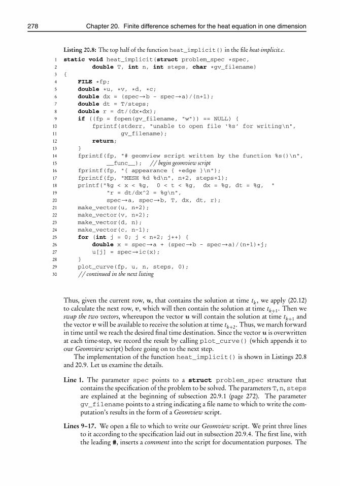
root2014/7/8page 278
�
�
�
�
�
�
�
�
278 Chapter 20. Finite difference schemes for the heat equation in one dimension
Listing 20.8: The top half of the function heat_implicit() in the file heat-implicit.c.
1 static void heat_implicit(struct problem_spec *spec,2 double T, int n, int steps, char *gv_filename)3 {4 FILE *fp;5 double *u, *v, *d, *c;6 double dx = (spec→b - spec→a)/(n+1);7 double dt = T/steps;8 double r = dt/(dx*dx);9 if ((fp = fopen(gv_filename, "w")) == NULL) {
10 fprintf(stderr, "unable to open file ‘%s’ for writing\n",11 gv_filename);12 return;13 }14 fprintf(fp, "# geomview script written by the function %s()\n",15 __func__); // begin geomview script16 fprintf(fp, "{ appearance { +edge }\n");17 fprintf(fp, "MESH %d %d\n", n+2, steps+1);18 printf("%g < x < %g, 0 < t < %g, dx = %g, dt = %g, "19 "r = dt/dx^2 = %g\n",20 spec→a, spec→b, T, dx, dt, r);21 make_vector(u, n+2);22 make_vector(v, n+2);23 make_vector(d, n);24 make_vector(c, n-1);25 for (int j = 0; j < n+2; j++) {26 double x = spec→a + (spec→b - spec→a)/(n+1)*j;27 u[j] = spec→ic(x);28 }29 plot_curve(fp, u, n, steps, 0);30 // continued in the next listing
Thus, given the current row, u, that contains the solution at time tk , we apply (20.12)to calculate the next row, v, which will then contain the solution at time tk+1. Then weswap the two vectors, whereupon the vector u will contain the solution at time tk+1 andthe vector v will be available to receive the solution at time tk+2. Thus, we march forwardin time until we reach the desired final time destination. Since the vector u is overwrittenat each time-step, we record the result by calling plot_curve() (which appends it toour Geomview script) before going on to the next step.
The implementation of the function heat_implicit() is shown in Listings 20.8and 20.9. Let us examine the details.
Line 1. The parameter spec points to a struct problem_spec structure thatcontains the specification of the problem to be solved. The parameters T, n, stepsare explained at the beginning of subsection 20.9.1 (page 272). The parametergv_filename points to a string indicating a file name to which to write the com-putation’s results in the form of a Geomview script.
Lines 9–17. We open a file to which to write our Geomview script. We print three linesto it according to the specification laid out in subsection 20.9.4. The first line, withthe leading #, inserts a comment into the script for documentation purposes. The

root2014/7/8page 279
�
�
�
�
�
�
�
�
20.9. The file heat-implicit.c 279
Listing 20.9: The bottom half of the function heat_implicit() in the file heat-implicit.c.
31 // continued from the previous listing32 for (int j = 0; j < n-1; j++)33 c[j] = -r;34 for (int k = 1; k ≤ steps; k++) {35 double *tmp;36 double t = T*k/steps;37 v[0] = spec→bcL(t);38 v[n+1] = spec→bcR(t);39 u[1] += r*v[0];40 u[n] += r*v[n+1];41 for (int i = 0; i < n; i++)42 d[i] = 1 + 2*r;43 trisolve(n, c, d, c, u+1, v+1);44 tmp = v;45 v = u;46 u = tmp;47 plot_curve(fp, u, n, steps, k);48 }49 fprintf(fp, "}\n"); // end geomview script50 fclose(fp);51 printf("geomview script written to file %s\n", gv_filename);52 if (spec→u_exact �= NULL) {53 double err = get_error(spec, u, n, T);54 printf("max error at time %g is %g\n", T, err);55 }56 free_vector(u);57 free_vector(v);58 free_vector(d);59 free_vector(c);60 putchar(’\n’);61 }
comment contains the name of the current function, that is, heat_implicit(),which is captured by the __func__ identifier. The __func__ identifier84 wasintroduced in C99. If you are limited to C89, then remove __func__ and hard-code the function name instead. You may remove or change that comment, or addmore such comment lines as you see fit; e.g., you may want to add your name andemail address. To add the current date, see the documentation of strftime() inthe standard library.
Line 18. We print a message to the stdout with the problem’s basic data for the user’sinformation. The transcript of the interactive session on page 266 shows how itmanifests.
Lines 21–24. We allocate memory for the solver’s working vectors. The vectors u and vare the current row and the next row vectors introduced earlier in this subsection.The vector d will hold the diagonal of the n × n tridiagonal matrix in (20.12)
84Since it may be difficult to discern in a typeset document, let me point out that there are two leading andtwo trailing underscores in __func__.

root2014/7/8page 280
�
�
�
�
�
�
�
�
280 Chapter 20. Finite difference schemes for the heat equation in one dimension
(page 257). The vector cwill hold both the subdiagonal and the superdiagonal sincethe two are the same in this case.
Lines 25–29. We initialize the vector u with the problem’s initial condition providedby the function spec→ic() and then call plot_curve() to insert that initialtime-slice into our geomview script.
Continuing on to Listing 20.9:
Line 32. We initialize the super/subdiagonal vector c in accordance with system (20.12).As noted in Remark 20.2 (page 274), the vector c does not change during the solvingprocess.
Lines 34–48. This is where the real action takes place. Given the current row u, it ap-plies (20.12) to compute the next row v and repeats. Let me point out a few sub-tleties.
Lines 37–38. The first and last entries of the vector v, that is, v[0] and v[n+1],fall on the domain’s boundary; therefore their values are read from the sup-plied boundary conditions.
Lines 39–40. We adjust the vector u by adding the rightmost column of (20.12)to it.
Line 41. We initialize the diagonal vector d to 1+ 2r , in accordance with (20.12).Unlike the vectorc, which is not changed bytrisolve(), the vectord does;therefore it needs to be refreshed upon each iterative pass.
Line 43. Having thus prepared the vectors u, v, c, and d, we pass them totrisolve() to solve the system (20.12). Although the state vectors u and vare of length n+2 each, the system (20.12) is only n×n since it updates internalnodes only! That’s the reason for passing u+1 and v+1 totrisolve(); theseskip the first elements of the two vectors. Their last elements are skipped aswell since trisolve() accesses only the first n entries of the vectors it re-ceives.
Lines 44–47. We swap the vectors u and v so that u now contains the problem’smost up-to-date state and then call plot_curve() to plot that time-slice.
The rest of the code is self-explanatory, so I won’t elaborate.
20.10 Project Finite Differences in One Dimension
Part 20.1. Implement, compile, and test heat-implicit.c.
Part 20.2. Copy heat-implicit.c to heat-explicit.c, and modify it to implement the explicitfinite difference scheme of Section 20.2. If r = Δt/(Δx)2 is greater than 0.5, print amessage warning the user of the scheme’s instability, but continue with the computationnevertheless.
Part 20.3. Copy heat-implicit.c to heat-crank-nicolson.c, and modify it to implement theCrank–Nicolson finite difference scheme of Section 20.4.

root2014/7/8page 281
�
�
�
�
�
�
�
�
20.10. Project Finite Differences in One Dimension 281
Part 20.4. Copy heat-implicit.c to heat-seidman-sweep.c, and modify it to implement theSeidman sweep finite difference scheme of Section 20.5.
You will find that unlike the previous iteration schemes that required a current rowand a next row (the vectors u and v), you will be working with just one vector. The mostobvious implementation of the Seidman scheme changes that vector in place as you sweepit from left to right and then from right to left.
Part 20.5. [optional] The function trisolve() computes the components of the vec-tor d[]; see Listing 20.5, line 6. That vector, however, does not change during the pro-gram’s execution. Therefore recomputing it upon every invocation of trisolve() iswasteful. See if you can change your program to compute d[] just once.
Part 20.6. [optional] Implement the suggestion of Remark 20.3.

root2014/7/8page 283
�
�
�
�
�
�
�
�
Chapter 21
The porous mediumequation
Prerequisites: Chapters 7, 8, 20
21.1 IntroductionThe porous medium equation
∂ u
∂ t=∂ 2u m
∂ x2 (m > 1) (21.1)
is a model of diffusion of a substance, typically gas, through a porous medium. The un-known u(x, t ) is the gas density at the point x at time t . The exponent m—which is notnecessarily an integer—is a physical property of the diffusing material. Equation (21.1)arises in other contexts as well. Have a look at this chapter’s appendix to see how it comesabout as a model in population dynamics. You will find a quite readable treatise on thesubject, along with an extensive bibliography, in Vázquez [77]. One thing you shouldknow is that if the initial condition u(x, 0) is nonnegative, then the solution u(x, t ) isnonnegative for all t > 0, and therefore the exponentiation makes sense in that case. SeeSection 21.3 for a generalization to solutions of varying sign.
The goal in this chapter is to develop a finite difference scheme to solve initial/boundary value problems corresponding to (21.1). As we will see, the Seidman sweepscheme introduced in Section 20.5 leads to quite a simple implementation.
21.2 Barenblatt’s solutionWhen m = 1, (21.1) reduces to the heat equation; cf. (20.1) on page 251. The conditionm > 1, however, makes the porous medium equation a totally different beast compared tothe heat equation. You may intuit a sign of trouble if you express (21.1) in the equivalentform ∂ u
∂ t =∂∂ x
�mu m−1 ∂ u
∂ x
, which makes it clear that it is a nonlinear diffusion equation,
as in ∂ u∂ t =
∂∂ x
�κ∂ u∂ x
, whose diffusion coefficient, κ = mu m−1, varies with the density.
Since m > 1, κ tends to zero as density tends to zero. Thus, the diffusion process degen-erates near zero densities. The porous medium equation is the archetype of the class ofdegenerate parabolic equations.
The bulk of the theory of parabolic equations concerns the nondegenerate case. Justabout everything breaks down when degeneracy occurs. One of the striking facts about
283

root2014/7/8page 284
�
�
�
�
�
�
�
�
284 Chapter 21. The porous medium equation
the porous medium equation—a consequence of the degeneracy—is that its solutions ex-hibit a finite speed of propagation into vacuum (i.e., a zero density region). This is verymuch in contrast to the heat equation whose solutions spread out at infinite speed. Thefinite speed of propagation is evident in the class of self-similar solutions to (21.1) con-structed by Barenblatt:
u(x, t ) =1
(t +δ)β
�2c − γ
* x
(t +δ)β
+23+
�α, −∞< x <∞, t ≥ 0, (21.2)
where
α=1
m− 1, β=
1
m+ 1, γ =
m− 1
2m(m+ 1),
and where c ≥ 0 and δ ≥ 0 are arbitrary constants. The notation [ · ]+ means max(·, 0).We see that at any time t > 0 the support85 of the solution is
|x|<√√√ c
γ(t +δ)β,
which propagates at a finite (but nonconstant) speed, as asserted.In the special case of m = 3, Barenblatt’s solution takes on a particularly simple form,
u(x, t ) =1
(t +δ)1/4
√√√√c − x2
12(t +δ)1/2, (21.3)
or equivalently,x2
12c(t +δ)1/2+
u2
c(t +δ)−1/2= 1.
Therefore, the graph of u versus x (for any fixed t ) is precisely the upper half of an ellipse
with semimajor and semiminor axes lengths of�
c(t +δ)−1/2 and�
12c(t +δ)1/2. Theellipse flattens and spreads out as t increases. The area under the ellipse, which is pro-portional to the mass of the diffusing substance, remains constant at
�3πc . Figure 21.1
shows snapshots of the graphs of u(x, t ) for several choices of t .Barenblatt’s solution is quite handy as a test case for our finite difference solver. We
set up a problem with initial and boundary data derived from Barenblatt’s solution, andthen we expect that the solution produced by our solver will agree with Barenblatt’s.
21.3 GeneralizationsSince the exponent m in (21.1) is not necessarily an integer, the expression u m is not welldefined if u is negative. The extension
∂ u
∂ t=∂ 2(|u|m−1 u)
∂ x2 (21.4)
of (21.1) admits negative u, is well-posed as a partial differential equation, and reducesto (21.1) when u is nonnegative. For this reason, most of the literature on the porous
85The support of a function is the closure of the set where it is nonzero.

root2014/7/8page 285
�
�
�
�
�
�
�
�
21.4. The finite difference scheme 285
x
u(x, t )
−1 − 25
0 25
1
1t0 = 0
t1 = 7/100
t2 = 203/400t3 = 4
Figure 21.1: These flattening and spreading ellipses are snapshots of Barenblatt’s solu-tion, (21.3), of the porous medium equation with m = 3 at various times.The parameters δ = 1/75 and c =
�3/15 are chosen so that the solution
at time t0 = 0 has amplitude 1 and support [−2/5,2/5]. I will leave it toyou to verify that (a) at time t1 = 7/100 the solution curve takes the formof a semicircle of radius
42/5, and (b) the solution front arrives at x =±1
at time t2 = 203/400. The solution curve at t3 = 4 is also shown to give abetter feel for how the solution spreads out in time.
medium equation addresses (21.4) rather than the special case (21.1). Yet a further gener-alization of (21.4) is the equation
∂ u
∂ t=∂ 2φ(u)
∂ x2 , (21.5)
where φ : R → R is some smooth monotonically increasing function with φ(0) = 0and φ′(0) = 0. Much of the theory pertaining to the porous medium equation may bedeveloped in the context of (21.5) with very minimal assumptions onφ. See, for instance,the articles [2, 9] and the book [77]. Clearly, (21.4) is the special case of (21.5) withφ(u) =|u|m−1u. I will state and explain this chapter’s algorithm in the context of (21.5) for thesake of generality but will drop to the simple case of (21.1) for illustrations.
21.4 The finite difference schemeThe porous medium equation’s counterpart of the initial/boundary value problem (20.2)is the following:
Find u = u(x, t ) so that
∂ u∂ t=∂ 2φ(u)
∂ x2 , x ∈ (a, b ), t > 0, (21.6a)
u(x, 0) = u0(x), x ∈ (a, b ), (21.6b)u(a, t ) = uL(t ), u(b , t ) = uR(t ), t > 0. (21.6c)
As in the case of Chapter 20’s heat equation, the initial condition u0(x) and the left andright boundary conditions uL(t ) and uR(t ) serve to define a unique solution u(x, t ) inthe semi-infinite strip a ≤ x ≤ b and t > 0 in the x-t plane. Also as before, in a finite

root2014/7/8page 286
�
�
�
�
�
�
�
�
286 Chapter 21. The porous medium equation
difference approximation we replace the interval a ≤ x ≤ b with a collection of n + 2equally spaced points x0 < x1 < · · · < xn+1, where x0 = a and xn+1 = b , and we letΔx = (b − a)/(n+ 1). Similarly, we discretize the time into “time-slices” t0 < t1 < t2 . . .,where t0 = 0, and the spacing between the slices is a prescribedΔt . Figure 20.2 on page 253shows the resulting finite difference grid.
In the rest of this section I will use the notation and ideas introduced in Section 20.5without further elaboration. The forward and reverse difference formulas (20.16) (onpage 261) now take the form
vj − uj =−r�φ(vj )−φ(vj−1)
− r�φ(uj )−φ(uj+1)
, j = 1,2, . . . , n, (21.7a)
wj − vj =−r�φ(vj )−φ(vj−1)
− r�φ(wj )−φ(wj+1)
, j = n, . . . , 2,1, (21.7b)
where
r =Δt
2(Δx)2,
as in (20.15). (I have changed the notation from r ′ to r here since there is no chance ofconfusion within this chapter.) We rearrange the equations (21.7) into
vj + rφ(vj ) = rφ(vj−1)+ uj − rφ(uj )+ rφ(uj+1), j = 1,2, . . . , n, (21.8a)
wj + rφ(wj ) = rφ(vj−1)+ vj − rφ(vj )+ rφ(wj+1), j = n, . . . , 2,1. (21.8b)
During the forward sweep, all the terms on the right-hand side of (21.8a) are known.We solve the nonlinear equation vj + rφ(vj )= “known” to find vj . Similarly, during thereverse sweep, all the terms on the right-hand side of (21.8b) are known. We solve the non-linear equation wj + rφ(wj ) = “known” to find wj . Thus, in comparison with the heatequation of Chapter 20, the only extra effort is in solving a nonlinear equation of theform ξ + rφ(ξ ) = c at each step. This may be accomplished through a Newton’s itera-tion without much trouble by starting with an initial guess ξ0. Sinceφ is expected to be amonotonically increasing function, any reasonable choice for ξ0 will do. I suggest takingξ0 = c and leave its implementation as an instructive project. In the rest of this chapter,however, I will focus on the special case of φ(u) = u3, which avoids Newton’s iterationaltogether. Here is why.
To solve the cubic equation ξ + rξ 3 = c for ξ , we multiply it through by r 1/2 to getr 1/2ξ + r 3/2ξ 3 = r 1/2c . Letting η= r 1/2ξ and k = r 1/2c , we arrive at the cubic equationη+η3 = k. You may verify that the unique real root of η+η3 = k has the explicit form
η=γ
6− 2
γ, where γ =
�108k + 12
412+ 81k2�1/3. (21.9)
Thus, we evaluate η and then set ξ = r−1/2η= η/�
r .
21.5 The programThe rest of this chapter is devoted to details of the implementations of the Seidman sweepfor solving the initial/boundary value problem (21.6) in the special case whenφ(u) = u3.The case of a general φ is left as a project.
Our program relies on xmalloc.[ch] from Chapter 7 to allocate memory and the filearray.h from Chapter 8 to construct vectors and matrices. Additionally, we will adaptthe previous chapter’s problem specification file, problem-spec.c, to the case in hand. Thefile problem-spec.h remains unchanged, so a symbolic link will do. Thus, following thesuggestions in Chapters 2 and 6, the contents of the project’s directory will look like this:

root2014/7/8page 287
�
�
�
�
�
�
�
�
21.5. The program 287
$ cd pme$ ls -FMakefile pme-seidman-sweep.c problem-spec.h@ [email protected] problem-spec.c xmalloc.c@
Here is a transcript of a sample interactive session:
$ ./pme-seidman-sweepUsage: ./pme-seidman-sweep T n s
T : solve over 0 ≤ t ≤ Tn : the number of grid points a=x[0], x[1], ... , x[n], x[n+1]=bs : the number of time slices 0=t[0], t[1], ... , t[s]=T
$ ./pme-seidman-sweep 1 20 20problem pme1:-1 < x < 1; 0 < t < 1, dx = 0.0952381,
dt = 0.05, r = dt/(2*dx^2) = 2.75625geomview script written to file pme1.gvmax error at time 1 is 0.013731
problem pme2:-1 < x < 1; 0 < t < 1, dx = 0.0952381,
dt = 0.05, r = dt/(2*dx^2) = 2.75625geomview script written to file pme2.gv
The program solves two initial/boundary value problems for the porous mediumequation, both with φ(u) = u3. These are the following:
Problem pme1: This produces a finite difference approximation to Barenblatt’s solu-tion (21.2) of the porous medium equation with m = 3, c =
�3/15, and δ = 1/75
on the bounded interval −1 ≤ x ≤ 1. The values of c and δ are chosen so thatthe initial condition (whose graph is the upper half of an ellipse) has amplitude 1and is supported on the interval [−2/5,−2/5]. Figure 21.1 shows snapshots of thesolution at a few selected times. Figure 21.2(left) shows the graph of the solutionu(x, t ) as a surface in three dimensions.
Implementing the problem involves writing a function to evaluate Barenblatt’s solu-tion u(x, t ) in (21.2) and then extracting its initial and boundary data by evaluatingu(x, 0) and u(±1, t ), as explained in the “reverse-engineering” idea in (20.19) onpage 264.
Problem pme2: This solves the initial/boundary value problem (21.6) on the interval−1≤ x ≤ 1 with the boundary data uL(t ) = uR(t )≡ 0 and the initial data
u0(x) =
⎧⎪⎨⎪⎩1/2 if 0< x < 1/2,−1/2 if − 1/2< x < 0,0 otherwise.
In particular, this tests the scheme’s ability to handle initial data of variable sign.Figure 21.2(right) shows the graph of the solution u(x, t ) as a surface in threedimensions.

root2014/7/8page 288
�
�
�
�
�
�
�
�
288 Chapter 21. The porous medium equation
Figure 21.2: Graphs of the solutions u(x, t ) of problemspme1 (left) and pme2 (right) assurfaces in three dimensions computed by our finite difference solver andrendered in Geomview. Compare the graph of pme1 to the correspondingsnapshots in Figure 21.1.
21.6 The files problem-spec.[ch]The file problem-spec.h is identical to the file of the same name in the previous chapter, so asymbolic link will do. The file problem-spec.c, which is shown in an outline in Listing 21.1,contains the specifications of problems pme1 and pme2. The function barenblatt()on line 3 implements Barenblatt’s solution (21.2), where m, c , and δ are given as param-eters. The function pme1_exact(), which is given in its entirety beginning on line 7,produces a special case of Barenblatt’s solution corresponding to m = 3, c =
�3/15, and
δ = 1/75. The functions pme1_ic(), pme1_bcL(), and pme1_bcR(), which yieldthe problem’s initial and boundary data, simply evaluate pme1_exact() at t = 0 andx = ±1. The function pme1() on line 15 is identical to the function heat1() givenon lines 23–35 of Listing 20.2 on page 271 except for all occurrences of “heat1” beingreplaced by “pme1”.
Similarly, functions pme2_ic(), pme2_ic(), pme2_bcL(), and pme2(), yieldthe problem specification of problem pme2 as described at the end of the previous sec-tion. You should have no problem in filling in the details. No exact solution is availablefor pme2.
21.7 The file pme-seidman-sweep.cThe file pme-seidman-sweep.c contains the implementation of the Seidman sweep schemefor solving the boundary value problem (21.6) assuming φ(u) = u3. The changes relativeto the file heat-seidman-sweep.c of Chapter 20, which I assume that you wrote and testedearlier, are quite minimal. In effect, we need just one extra function, let’s call it croot(),to solve the cubic equation η+η3 = k according to the formula (21.9). Here it is:
1 static double croot(double k)2 {3 double s = sqrt(12 + 81*k*k);4 double gamma = pow(108*k + 12*s, 1.0/3);5 return gamma/6 - 2/gamma;6 }
root2014/7/8page 289
�
�
�
�
�
�
�
�
21.9. Appendix: The porous medium equation as a population dynamics model 289
Listing 21.1: An outline of the file problem-spec.c.
1 #include ...2 // Barenblatt’s solution3 � static double barenblatt(double x, double t, double m,4 double c, double delta) ...5
6 // pme1: Barenblatt’s solution with m = 3, and special choices of c and δ7 static double pme1_exact(double x, double t)8 {9 double c = sqrt(3)/15, delta = 1.0/75;
10 return barenblatt(x, t, 3, c, delta);11 }12 � static double pme1_ic(double x) ...13 � static double pme1_bcL(double t) ...14 � static double pme1_bcR(double t) ...15 � struct problem_spec *pme1(void) ...16
17 // pme2: initial condition with variable sign18 � static double pme2_ic(double x) ...19 � static double pme2_bcL(double t) ...20 � static double pme2_bcR(double t) ...21 � struct problem_spec *pme2(void) ...
The for-loops that actually perform the forward or reverse sweeps are only slightlydifferent from their Chapter 20 counterparts. Calculating vj or wj out of equations (20.17)(page 261) requires only a division by 1+ r ′. Calculating vj or wj out of equations (21.8)(page 286) calls for solving a cubic equation. We have croot() to do that. Problemsolved.
21.8 Project Porous Medium
Part 21.1. Copy the files problem-spec.c and heat-seidman-sweep.c from Chapter 20 tothe current project’s directory, and modify them as instructed above to produce a finitedifference solver for the porous medium equation (21.6) with φ(u) = u3.
Part 21.2. [Optional] Modify your program to handle a general φ : R→ R assumingφ(0) = 0 andφ is monotonically increasing. You will replace the function croot()witha solver (using Newton’s iteration) for the equation ξ + rφ(ξ ) = c .
21.9 Appendix: The porous medium equation as a populationdynamics modelIt is not out of place to show how (21.6a) arises out of a simple population model. Al-though the treatment of this chapter has been limited to a one-dimensional space, thederivation of the model works more transparently in an n-dimensional setting, and that’swhat I will do. At the very end you may set n = 1 if you like.
Consider a certain hypothetical population that lives in the n-dimensional space Rn .Assume that there exists a population density function u(x, t ) so that the population in any
root2014/7/8page 290
�
�
�
�
�
�
�
�
290 Chapter 21. The porous medium equation
arbitrary regionω ⊂Rn at time t is given by∫ω
u(x, t )dx. Also assume that there existsa vector function v(x, t ) that gives the velocity of the movement of the individuals at thepoint x at time t . For simplicity’s sake, let’s assume that the members of the populationdon’t reproduce and don’t die. Then the rate of increase of the population in ω equalsexactly the inflow of the population through its boundary, that is,
d
d t
∫ω
u dx=−∫∂ ω
uv ·nda,
where n is the outward unit normal to the boundary ∂ ω of ω.We move the time derivative to under the integration sign. That’s permissible since
ω is independent of time. On the right-hand side, we may apply the Divergence Theorem(see, e.g., the section titled “Curl and Divergence” in Stewart [65]) from multivariablecalculus to change the boundary integral to a volume integral. We get∫
ω
∂ u∂ t
dx=−∫ω
div(uv)da.
Sinceω is arbitrary, we conclude that
∂ u∂ t+ div(uv) = 0.
What we have obtained is the equation of conservation of mass. That we derived it in thecontext of population dynamics is quite irrelevant. The density u and velocity v couldhave been those of the exhaust gases of a rocket, the air flowing around an airplane’s wings,blood coursing through an animal’s veins, or a vibrating metal plate. The equation of theconservation of mass links a material’s velocity and density functions, assuming that thematerial is neither created nor destroyed.
Returning to the population model, assume that the species are averse to living in highdensity areas. More precisely, if the population density is not constant in a particularindividual’s neighborhood, the individual runs to a lower density area; that is, it movesin the opposite direction of the density gradient,∇u, and the speed of the movement is afunction of the density itself, let’s say v =−ψ(u)∇u. Substituting this in the equation ofconservation of mass results in
∂ u∂ t= div
�uψ(u)∇u
�.
To connect this to the porous medium equation, introduce a function φ through φ(u) =∫ u0 σψ(σ)dσ , that is, φ′(u) = uψ(u) andφ(0) = 0. Then the expression inside the square
brackets becomes φ′(u)∇u, that is, ∇φ(u), and we conclude that
∂ u
∂ t= div∇φ(u) =∇2φ(u).
In the one-dimensional case this reduces to (21.6a).

root2014/7/8page 291
�
�
�
�
�
�
�
�
Chapter 22
Gaussian quadrature
Prerequisites: None
22.1 IntroductionThe Gaussian quadrature algorithm gives the optimal distribution of integration pointsand weights for integrating numerically a function of one variable on an interval. Specif-ically, an n-point quadrature rule on the interval (−1,1) selects n points {xj }n
j=1, andweights {wj }n
j=1, so that for all reasonably nice functions f (x) defined on (−1,1) one has∫ 1
−1f (x)d x ≈
n∑j=1
wj f (xj ). (22.1)
The interval (−1,1) is the natural setting for developing the theory of the Gaussian quadra-ture, but that does not limit the algorithm’s applicability; integrals on arbitrary intervals(a, b )may be reduced to integrals on (−1,1) through a change of variables:∫ b
af (x)d x =
b − a
2
∫ 1
−1f�
b + a
2+
b − a
2ξ
�dξ (22.2a)
=b − a
2
∫ 1
−1f�
a2(1− ξ )+ b
2(1+ ξ )
�dξ . (22.2b)
The two forms shown are obviously equivalent. Pick whichever you like.To get a feel for what is meant by the “optimal distribution of integration points and
weights” in this section’s opening paragraph, let us consider the following (very) trivialthought experiment. Suppose we are interested in integrating constant functions only,that is, functions f (x) such that f (x) ≡ c for some c , independently of x. In that case∫ 1−1 f (x)d x = 2c = 2 f (x∗). Any x∗ will do since f is constant. Comparing to (22.1), this
corresponds to a 1-point quadrature (n = 1), with w1 = 2 and x1 = x∗.There is no question that the formula 2 f (x∗) gives exact results when f is constant.
Also, there is no question that the formula 2 f (x∗)won’t work for nonconstant functions.Or will it? What if f (x) = c0+ c1 x for some constants c0 and c1? Then we have∫ 1
−1f (x)d x =
∫ 1
−1(c0+ c1x)d x =
�c0x +
1
2c1x2
������1
−1
= 2c0 = 2 f (0).
291
root2014/7/8page 292
�
�
�
�
�
�
�
�
292 Chapter 22. Gaussian quadrature
Surprise! The one-point quadrature rule with w1 = 2 and x1 = 0 gives exact results for allfunctions f (x) = c0+ c1x.
In contrasting the two cases considered so far, we see that the one-point quadrature for-mula is able to integrate identically constant functions exactly. The choice of the quadra-ture point x1 = x∗ is immaterial. However, the special choice of x1 = 0 enables it toproduce, as a bonus, the exact integrals of the nonconstant functions f (x) = c0 + c1x aswell. This is the meaning of the “optimal distribution of integration points and weights”noted earlier. This observation generalizes in the following ways:
1. To any arbitrary choice of n distinct points {xj }nj=1 in the interval (−1,1), there
corresponds weights {wj }nj=1 so that
∫ 1
−1p(x)d x =
n∑j=1
wj p(xj ) for all polynomials p of degree n− 1. (22.3)
2. There exists a special choice of n points {xj }nj=1 in the interval (−1,1), and weights
{wj }nj=1, so that
∫ 1
−1p(x)d x =
n∑j=1
wj p(xj ) for all polynomials p of degree 2n− 1. (22.4)
We will justify these statements in sections 22.2 and 22.4. For now, let us note that thespecial choice of quadrature points yields a bonus whereby the quadrature’s applicabilityextends from polynomials of degree n − 1 to polynomials of degree 2n − 1. The earlierexamples with f (x)≡ c and f (x) = c0+c1x correspond to the case n = 1 of the statementsabove. There, the special choice of x∗ = 0 extended the quadrature’s applicability frompolynomials of degree 0 to polynomials of degree 1.
Gaussian quadrature refers to the special choice of points and weights noted above.It is the goal of this chapter to explain some of the mathematics behind the Gaussianquadrature and then produce a C module that yields the lists of points and weights of aGaussian quadrature of a desired degree on demand.
Remark 22.1. More often than not, we use Gaussian quadrature to integrate functionsother than polynomials. In that case we obtain an approximation to the true value of theintegral: ∫ 1
−1f (x)d x ≈
n∑j=1
wj f (xj ).
The accuracy of the result depends on how close the function f is to a degree 2n − 1polynomial. For detailed error estimates see [4, 28].
22.2 Lagrange interpolationA generic polynomial p(x) = c0 + c1x + c2x2 + · · · + cn−1 xn−1 of degree n − 1 in x isdetermined by its n coefficients {ci}n−1
i=0 . It is within reason then to expect that a set ofcoefficients may be found so that yi = p(xi ), i = 1,2, . . . , n, where
,(xi , yi )
-ni=1 are given,
and the xi ’s are distinct.

root2014/7/8page 293
�
�
�
�
�
�
�
�
22.2. Lagrange interpolation 293
−3 −2 −1 1 2 3
−1
1
x
�5(x)
Figure 22.1: The graph of the sixth degree polynomial �5(x), with the property that�5(x) = 0 for x =−3,−2,−1,0,2,3, and �5(1) = 1.
The brute force method of obtaining the coefficients {ci}n−1i=0 is by solving the system
of n linear equations yi = p(xi ) in the n unknowns ci . The clever way of obtaining thecoefficients is through Lagrange interpolation. To do the latter, consider the product
π j (x) =n∏
i=1i �= j
(x − xi ) = (x − x1) · · · (x − xj−1)(x − xj+1) · · · (x− xn )
for j = 1,2, . . . , n, and note that π j (x) is a polynomial of degree n−1 in x, andπ j (xi ) = 0for all i except for i = j , when it equals
π j (xj ) =n∏
i=1i �= j
(xj − xi ) = (xj − x1) · · · (xj − xj−1)(xj − xj+1) · · · (xj − xn).
It follows that the function
� j (x) =
n∏i=1i �= j
(x − xi )
n∏i=1i �= j
(xj − xi )=(x − x1) · · · (x − xj−1)(x− xj+1) · · · (x− xn )
(xj − x1) · · · (xj − xj−1)(xj − xj+1) · · · (xj − xn)
is polynomial of degree n− 1 in x, and
� j (xi ) =�
0 if i �= j ,1 if i = j .
(22.5)
For instance, let the coordinates xi be selected as the sequence of the seven values
[−3,−2,−1,0,1,2,3].
Since x5 = 1, we have
�5(x) =1
48(x+ 3)(x + 2)(x + 1)x(x − 2)(x − 3) (note: no (x − 1) term!).
Figure 22.1 shows the graph of the sixth degree polynomial �5(x). Note that �5(x) is zerowhen x ∈ {−3,−2,−1,0,2,3}, and �5(1) = 1, as expected.

root2014/7/8page 294
�
�
�
�
�
�
�
�
294 Chapter 22. Gaussian quadrature
Going back to the problem of determining the polynomial p(x) of degree n − 1 sothat yi = p(xi ) for i = 1,2, . . . , n, it’s clear that
p(x) =n∑
j=1
� j (x)yj (22.6)
fits the bill since it is of degree n− 1, and p(xi ) = yi due to (22.5).The polynomial p(x) constructed above is unique. To see why, suppose that there
is another n − 1 degree polynomial, q(x), such that yi = q(xi ) for i = 1,2, . . . , n. Letr (x) = p(x)− q(x). Then we have r (xi ) = 0 for all i = 1,2, . . . , n. Thus, the n− 1 degreepolynomial r has n roots. By the Fundamental Theorem of Algebra that can happen onlyif r (x) is identically zero. It follows that p(x)≡ q(x).
Equation (22.6) is called Lagrange’s interpolation formula. It is important to note thatthe functions � j (x) do not depend on the yj ’s. The yj ’s appear only as coefficients in (22.6).Furthermore, since yi = p(xi ), it is convenient to express (22.6) in the form
p(x) =n∑
j=1
� j (x)p(xj ), (22.7)
which removes the yj ’s from the picture altogether. Then integrating over the interval(−1,1) we arrive at∫ 1
−1p(x)d x =
n∑j=1
�∫ 1
−1� j (x)d x
�p(xj ) for all polynomials p of degree n− 1. (22.8)
If we define the constants wj according to
wj =∫ 1
−1� j (x)d x, j = 1,2, . . . , n,
then (22.8) exactly agrees with, and therefore proves, the statement (22.3).
22.3 Legendre polynomialsThe inner product of two functions f and g over the interval (−1,1) is defined by
( f , g ) =∫ 1
−1f (x)g (x)d x.
The inner product extends the idea of the dot product of vectors to functions. The func-tions f and g are said to be orthogonal if ( f , g ) = 0. For instance, if f (x) ≡ 1, g (x) = x,and h(x) = x2, then ( f , g ) =
∫ 1−1 x d x = 0, and therefore f and g are orthogonal. On the
other hand, ( f , h) =∫ 1−1 x2 d x = 2
3 �= 0, and therefore f and h are not orthogonal.Starting with the sequence of monomials 1, x, x2, x3, . . ., we may apply the Gram–
Schmidt orthogonalization procedure—see any textbook on linear algebra—to produce asequence of orthogonal functions. The sequence of polynomials thus generated are calledLegendre polynomials, the first few of which are
P0(x) = 1, P1(x) = x, P2(x) =1
2(3x2− 1), P3(x) =
1
2(5x3− 3x),
P4(x) =1
8(35x4− 30x2+ 3), P5(x) =
1
8(635− 70x3+ 15x).

root2014/7/8page 295
�
�
�
�
�
�
�
�
22.4. The Gaussian quadrature formula 295
−1 −0.5 0.5 1
−1
−0.5
0.5
1
x
Pn(x)
Figure 22.2: The graphs of the Legendre polynomials Pn(x) for n = 0,1,2,3,4.
The orthogonality relationship is
(Pm , Pn) =∫ 1
−1Pm(x)Pn(x)d x =
�0 if m �= n,
22n+1 if m = n.
There is a vast literature on the study of orthogonal polynomials, of which the Legen-dre polynomials are a very special case. If you are interested in learning more about these,Szego [73] is a good starting point. You will find simplified presentations of some of therelevant concepts in the books by Atkinson [4] (particularly, equations (4.4.21), (4.4.26),and (5.3.28)) and Hildebrand [28] (particularly, equations (7.6.9), (8.5.5), and (8.5.8)). Itturns out that for any n, the Legendre polynomial Pn(x) has n distinct real roots, all ofwhich lie in the interval (−1,1). Figure 22.2 shows the graphs of the first few Legendrepolynomials.
Furthermore, it is possible to show that the Legendre polynomials and their deriva-tives satisfy the recursion equations
(n+ 1)Pn+1(x) = (2n+ 1)xPn(x)− nPn−1(x), (22.9a)
(x2− 1)P ′n(x) = nxPn(x)− nPn−1(x). (22.9b)
These, together with P0(x)≡ 1 and P1(x) = x, provide a practical way of evaluating Pn(x)and P ′n(x) for all n and x.
22.4 The Gaussian quadrature formulaConsider a polynomial p(x) of degree 2n − 1 for some integer n ≥ 1. By applying theEuclidean long division algorithm to the fraction p(x)/Pn (x), we obtain
p(x)Pn(x)
= q(x)+r (x)
Pn(x),
where the quotient q(x) and the remainder r (x) are polynomials of degree n − 1 each.Rearranging the terms, we get
p(x) = Pn(x)q(x)+ r (x). (22.10)

root2014/7/8page 296
�
�
�
�
�
�
�
�
296 Chapter 22. Gaussian quadrature
Table 22.1: The coordinates xj and weights wj of the 4-point Gaussian quadrature.
j x j wj
1 −0.86113631159405257522 0.347854845137453857372 −0.33998104358485626480 0.652145154862546142633 0.33998104358485626480 0.652145154862546142634 0.86113631159405257522 0.34785484513745385737
Therefore ∫ 1
−1p(x)d x = (Pn , q)+
∫ 1
−1r (x)d x.
The inner product (Pn , q) is zero since the nth degree polynomial Pn(x) is orthogonalto all lower degree polynomials. Thus, the problem of integrating the (2n − 1)-degreepolynomial p(x) reduces to the problem of integrating the (n − 1)-degree polynomialr (x). The latter problem, however, was thoroughly analyzed in Section 22.2 and led tothe statement (22.8). Thus, we have∫ 1
−1p(x)d x =
n∑j=1
�∫ 1
−1� j (x)d x
�r (xj ). (22.11)
Up to this point, the evaluation points x1, x2, . . . , xn have been arbitrary. Magic hap-pens when we choose those to be the roots of the nth degree polynomial Pn(x), that is,Pn(xj ) = 0, j = 1,2, . . . , n. Then (22.10) indicates that p(xj ) = r (xj ) for all j ; there-fore (22.11) takes the form∫ 1
−1p(x)d x =
n∑j=1
�∫ 1
−1� j (x)d x
�p(xj ) for all polynomials p of degree 2n− 1,
which proves the statement (22.4).The integral of � j (x), which yields the quadrature’s weights wj , may be evaluated in
terms of the Legendre polynomials and their derivatives:
wj =∫ 1
−1� j (x)d x =
−2
(n+ 1)P ′n(xj )Pn+1(xj )=
2
(1− x2j )P
′n(xj )
2 , j = 1,2, . . . , n.
See, e.g., Atkinson [4, page 276, equation (5.3.28)] and Hildebrand [28, page 391, equa-tions (8.5.5) and (8.5.8)].
As a practical matter, the polynomial Pn(x) and its derivative P ′n(x) may be evalu-ated through the recursion formulas in (22.9). Then Newton’s method may be appliedto compute the roots xj of Pn(x). This supplies everything that is needed for evaluatingthe weights wj from the formulas given above. See Numerical Recipes in C [53] for animplementation in C. Table 22.1 shows the coordinates xj and weights wj of the 4-pointGaussian quadrature for illustration.
22.5 The programAs noted above, it is possible to write a C program to compute the Gaussian quadraturecoordinates xj and the corresponding weights wj on demand. However, since the com-puted data is static/unchanging, it makes better sense to compute them once for all and

root2014/7/8page 297
�
�
�
�
�
�
�
�
22.6. The files gauss-quad.[ch] 297
Listing 22.1: An interactive session with the gauss-quad-demo program. The five problems that aresolved here are described in this chapter’s Projects section.
$ ./gauss-quad-demoUsage: ./gauss-quad-demo n
n = number of quadrature points
$ ./gauss-quad-demo 2integrating a cubic function over (-1, 1)exact = 2.6666666666666665computed = 2.6666666666666665
integrating a cubic function over (2, 5)exact = 204.7500000000000000computed = 204.7500000000000000
integrating a quadratic function over (-1,1) x (-1,1)exact = 6.66666666666666696computed = 6.66666666666666607
integrating a quadratic function over (-1, 2) x (-1, 5)exact = 208.00000000000000000computed = 208.00000000000000000
integrating sin(x) over (0, 3.14159)exact = 2.0000000000000000computed = 1.9358195746511373
save them for future use. I have done that and have made the data file available at thisbook’s website in the files gauss-quad.[ch]. Your job is to write a driver, let’s call it gauss-quad-demo.c, to demonstrate the use of that data by performing a few integrations. Thisproject’s directory, therefore, will look like this:
$ cd gauss-quad$ ls -FMakefile gauss-quad-demo.c gauss-quad.c gauss-quad.h
My gauss-quad-demo.c contains five demonstrations. They are described in this chapter’sProjects section. You are encouraged to modify these or add demonstrations of your own.Listing 22.1 shows a transcript of an interactive session.
22.6 The files gauss-quad.[ch]I have computed the coordinates and weights of n-point Gaussian quadratures for n =1, . . . , 15 and placed them in the file gauss-quad.c, which you may download from thisbook’s website. I did the calculations in Maple with 40 digits of accuracy and then printedthe results with 20 digits of accuracy, as in "%.20f". The associated header file gauss-quad.h declares a structure
struct Gauss_qdat {double p; // pointdouble w; // weight
};
root2014/7/8page 298
�
�
�
�
�
�
�
�
298 Chapter 22. Gaussian quadrature
that holds a point/weight pair. An n-point quadrature table may be stored in an arrayof length n of such structures. I do, however, store the table in an array of length n+ 1.The (n+1)st extra entry is a dummy {0.0, -1.0} point/weight pair which serves as thetable’s terminal sentinel. In scanning the table, we recognize the sentinel by its negativeweight value since the normal Gauss quadrature weights are never negative. The inclu-sion of sentinel is by no means essential. I have introduced it merely for computationalconvenience. You will see its use in the code fragment at the end of this section.
In view of this, Table 22.1’s 4-point quadrature data is then encoded as the C structure:
static struct Gauss_qdat quaddata4[] = { /∗ n = 4 ∗/{ -0.86113631159405257522, 0.34785484513745385737},{ -0.33998104358485626480, 0.65214515486254614263},{ 0.33998104358485626480, 0.65214515486254614263},{ 0.86113631159405257522, 0.34785484513745385737},{ 0.0, -1.0},
};
This is one of the 15 quadrature tables defined in gauss-quad.c; they provide quadraturedata for n-point Gaussian quadratures for any n = 1,2, . . . , 15. The tables are namedquaddata1[], quaddata2[], . . . , quaddata15[].
To provide further organization to the data tables, I have defined an array, calledQuadTables[], each of whose entries points to one of the data tables:
static struct Gauss_qdat *QuadTables[] = {NULL, // no 0-point quadraturequaddata1,quaddata2,...quaddata15
};
Thus, Gauss_qdat[n] evaluates to a pointer to the n-point quadrature table.You may observe that the quadrature tables and the QuadTables[] array are all
specified static; therefore they are not directly accessible outside gauss-quad.c. Accessto the data is provided through the front-end function gauss_qdat(), which is definedin gauss-quad.c as
struct Gauss_qdat *gauss_qdat(int *n){
int ntables = (sizeof QuadTables / sizeof QuadTables[0]) - 1;if (*n < 1)
*n = 1;else if (*n > ntables)
*n = ntables;return QuadTables[*n];
}
The function begins with calculating ntables, which is the number of available quadra-ture tables. (See Remark 4.2 on page 22 for an explanation of that calculation.) We knowthat there are 15 tables, but that number is not hard-coded in the function since it maychange in the future.
The parameter n points to an integer n which the caller sets as the number of desiredquadrature points. If the requested number falls outside the 1 ... ntables range,it is brought into the range first (silently), and then a pointer to an appropriate table isreturned to the caller. Since the value stored in *nmay have to be changed during this call,

root2014/7/8page 299
�
�
�
�
�
�
�
�
22.7. Project Gaussian Quadrature 299
the function receives a pointer to an integer rather than an integer in its argument. Thecaller may examine the value of *n after the function returns if that value is of concern.
The following code fragment illustrates the use of our quadrature tables in integratinga function f over the interval [−1,1]:struct Gauss_qdat *gqdat;int n = 10; // want a 10-point quadraturegqdat = gauss_qdat(&n); // get the quadrature tablesum = 0.0;for (int i = 0; i < n; i++)
sum += gqdat[i].w * f(gqdat[i].p);printf("integral = %g\n", sum);
Alternatively, we may use the table’s sentinel for the stopping criterion:struct Gauss_qdat *gqdat;int n = 10; // want a 10-point quadraturegqdat = gauss_qdat(&n); // get the quadrature tablesum = 0.0;while (gqdat→w �= -1) { // watch for the sentinel
sum += gqdat→w * f(gqdat→p);gqdat++;
}printf("integral = %g\n", sum);
I (slightly) prefer the second version’s index-free code, but that’s a matter of taste. Dowhichever way that makes better sense to you.
22.7 Project Gaussian Quadrature
Part 22.1. Write a program gauss-quad-demo.c which reads the number n of quadraturepoints from the command-line and applies Gaussian quadrature to integrate the cubicfunction f (x) = 1+ x + x2 + x3 over the interval [−1,1]. The exact answer is 8/3. Canyou tell, before running your program, the minimal number of quadrature points thatwould produce the exact answer within the machine’s floating point accuracy?
Part 22.2. Extend gauss-quad-demo.c to compute, additionally, the integral of the pre-vious part’s f over the interval [2,5]. You will use one or the other of the change ofvariables formulas in (22.2). The exact answer is 819/4= 204.75.
Part 22.3. According to Fubini’s Theorem, the double integral over the square [−1,1]×[−1,1]may be expressed as nested single integrals:∫ 1
−1
∫ 1
−1f (x, y)d x d y =
∫ 1
−1
!∫ 1
−1f (x, y)d x
$d y.
If we approximate each of the single integrals on the right-hand side through a Gaussianquadrature, we get∫ 1
−1
∫ 1
−1f (x, y)d x d y ≈
m∑i=1
wi
* n∑j=1
wj f (xj , yi )+=
m∑i=1
n∑j=1
wi wj f (xj , yi ).
Extend gauss-quad-demo.c to apply the Gaussian quadrature with m = n to approximatethe integral of the quadratic function g (x, y) = 1+ x + y + x2 + xy + y2 over the square[−1,1]× [−1,1]. The exact answer is 20/3.

root2014/7/8page 300
�
�
�
�
�
�
�
�
300 Chapter 22. Gaussian quadrature
Part 22.4. Extend gauss-quad-demo.c to integrate the previous part’s g over the rectangle[−1,2]× [1,5]. The exact answer is 208.
Part 22.5. Extend gauss-quad-demo.c to compute∫ π
0 sin x d x. The exact answer is 2.Since the integrand is not a polynomial, a Gaussian quadrature can only produce an ap-proximate answer. Examine the answer’s accuracy as the number of quadrature pointsincreases. Note: Don’t hard-code the numerical value of π in your program. Instead, use4*atan(1).
root2014/7/8page 301
�
�
�
�
�
�
�
�
Chapter 23
Triangulation with theTriangle library
Prerequisites: Chapters 7, 8
23.1 IntroductionTriangulating a planar polygonal domain means dividing the domain into a union of tri-angles so that
1. every triangle has a nonempty interior;2. no two triangles have common interior parts; and3. any side of any triangle is either a part of the domain’s boundary or is the side of
another triangle.
Figure 23.1 shows sample triangulations. We see that a polygonal domain may have anumber of holes. Thus, a “polygonal domain” means a planar region bounded by one ormore nonintersecting polygonal boundaries.
A triangulated domain is also called a triangular mesh. A “mesh” is a more generalconcept than triangulation; one may have a mesh consisting of quadrilaterals or hexagons,for example. In this book we will work with triangular meshes only; therefore when I saya “mesh”, I mean a triangular mesh.
Triangulated domains are used frequently in the finite element method (FEM) forsolving partial differential equations (PDEs). (More on that in Chapter 25.) Stated veryloosely, the solution to the PDE is approximated by a low degree polynomial on eachtriangle. The FEM sees to it that the polynomial patches connect continuously across ad-jacent edges. The coefficients of the polynomials are adjusted to obtain the best possiblesolution.
Producing good triangulations is a complicated matter and an active area of research.A good triangulation—the technical term is a “quality triangulation”—produces triangleswhose angles are neither too small nor too large. We don’t want needle-like triangles; theaccuracy of the finite element approximation depends on that.
Triangle is a C library written by Jonathan Shewchuk [60, 61] for producing qual-ity triangulations of planar polygons, possibly with holes. It is available in source formfrom <https://www.cs.cmu.edu/~quake/triangle.html>. We will use Triangle formeshing in this and subsequent chapters. See Section 23.7 on how to install Triangle inyour working environment.
301
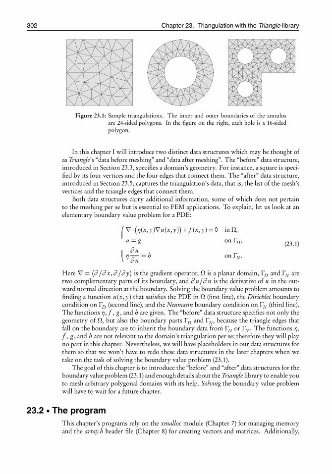
root2014/7/8page 302
�
�
�
�
�
�
�
�
302 Chapter 23. Triangulation with the Triangle library
Figure 23.1: Sample triangulations. The inner and outer boundaries of the annulusare 24-sided polygons. In the figure on the right, each hole is a 16-sidedpolygon.
In this chapter I will introduce two distinct data structures which may be thought ofas Triangle’s “data before meshing” and “data after meshing”. The “before” data structure,introduced in Section 23.3, specifies a domain’s geometry. For instance, a square is speci-fied by its four vertices and the four edges that connect them. The “after” data structure,introduced in Section 23.5, captures the triangulation’s data, that is, the list of the mesh’svertices and the triangle edges that connect them.
Both data structures carry additional information, some of which does not pertainto the meshing per se but is essential to FEM applications. To explain, let us look at anelementary boundary value problem for a PDE:⎧⎪⎪⎪⎨⎪⎪⎪⎩
∇ · �η(x, y)∇u(x, y) + f (x, y) = 0 in Ω,
u = g on ΓD ,
η∂ u∂ n= h on ΓN .
(23.1)
Here ∇ = ⟨∂ /∂ x,∂ /∂ y⟩ is the gradient operator, Ω is a planar domain, ΓD and ΓN aretwo complementary parts of its boundary, and ∂ u/∂ n is the derivative of u in the out-ward normal direction at the boundary. Solving the boundary value problem amounts tofinding a function u(x, y) that satisfies the PDE in Ω (first line), the Dirichlet boundarycondition on ΓD (second line), and the Neumann boundary condition on ΓN (third line).The functions η, f , g , and h are given. The “before” data structure specifies not only thegeometry of Ω, but also the boundary parts ΓD and ΓN , because the triangle edges thatfall on the boundary are to inherit the boundary data from ΓD or ΓN . The functions η,f , g , and h are not relevant to the domain’s triangulation per se; therefore they will playno part in this chapter. Nevertheless, we will have placeholders in our data structures forthem so that we won’t have to redo these data structures in the later chapters when wetake on the task of solving the boundary value problem (23.1).
The goal of this chapter is to introduce the “before” and “after” data structures for theboundary value problem (23.1) and enough details about the Triangle library to enable youto mesh arbitrary polygonal domains with its help. Solving the boundary value problemwill have to wait for a future chapter.
23.2 The programThis chapter’s programs rely on the xmalloc module (Chapter 7) for managing memoryand the array.h header file (Chapter 8) for creating vectors and matrices. Additionally,
root2014/7/8page 303
�
�
�
�
�
�
�
�
23.3. The file problem-spec.h 303
you will need the files triangle.[ch], mesh-to-eps.[ch], and mesh.c from the book’s website.I will describe their purposes later. Then, following the suggestions in Chapters 2 and 6,the initial state of this project’s directory will look like
$ cd meshing$ ls -FMakefile mesh-to-eps.h problem-spec.h [email protected]@ mesh.c [email protected] mesh.h [email protected] problem-spec.c xmalloc.c@
You will write mesh.h, problem-spec.[ch], and mesh-demo.c as you read through this chap-ter. The symbolic links triangle.[ho] are explained in Section 23.7.
Let us say the program compiles into the executable file mesh-demo. Here is a transcriptof a sample session:
$ ./mesh-demoUsage: ./mesh-demo a
a = maximal triangle area
$ ./mesh-demo 0.02domain is a squarevertices = 52, edges = 130, elems = 79PostScript output written to file square.eps
domain is a triangle with holevertices = 90, edges = 220, elems = 130PostScript output written to file triangle-with-hole.eps
domain is an annulus (really a 24-gon) of radii 0.325 and 0.65vertices = 74, edges = 174, elems = 100PostScript output written to file annulus.eps
domain is an L-shape with three holes (actually 16-gonsvertices = 141, edges = 349, elems = 206PostScript output written to file three-holes.eps
In the first attempt, the program is invoked without an argument. It writes a messagesaying that it expects an argument a which prescribes the maximal triangle area whichsets an upper bound on the areas of the mesh’s triangles and thus controls the finenessof the mesh. In the second attempt the program is invoked with an argument of 0.02.We see in the transcript that it meshes four distinct domains and prints the numbers ofvertices, edges, and elements in each case. An “element” in this context means a triangle;that’s a harbinger of future uses of this utility for FEM analysis.
Additional information in the transcript indicates that the program writes an imageof each mesh into a PostScript file. These may be viewed with any PostScript viewer.
23.3 The file problem-spec.hIt was noted in Section 23.1 that the program deals with separate “before meshing” and“after meshing” data structures. In this and the next section I will describe the former. InSection 23.5 I will describe the latter.
The “before meshing” data structure is called “struct problem_spec” because itcarries a problem specification. It is declared in the file problem-spec.h, which is shown inits entirety in Listing 23.1. Let us see what we have there:
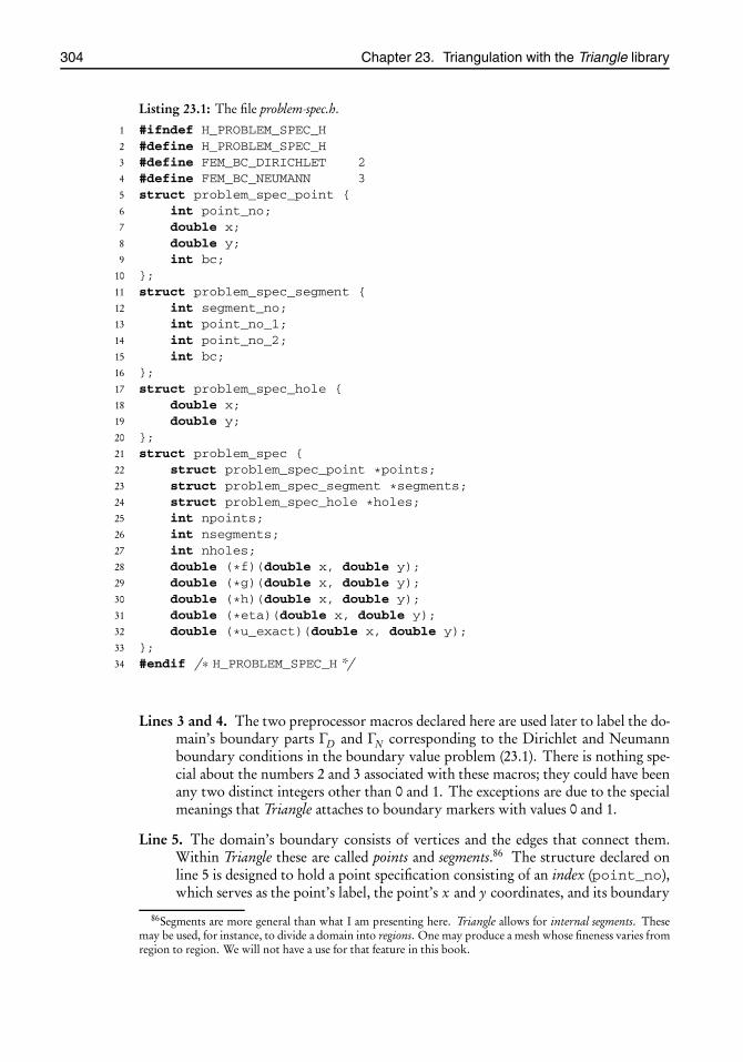
root2014/7/8page 304
�
�
�
�
�
�
�
�
304 Chapter 23. Triangulation with the Triangle library
Listing 23.1: The file problem-spec.h.
1 #ifndef H_PROBLEM_SPEC_H2 #define H_PROBLEM_SPEC_H3 #define FEM_BC_DIRICHLET 24 #define FEM_BC_NEUMANN 35 struct problem_spec_point {6 int point_no;7 double x;8 double y;9 int bc;
10 };11 struct problem_spec_segment {12 int segment_no;13 int point_no_1;14 int point_no_2;15 int bc;16 };17 struct problem_spec_hole {18 double x;19 double y;20 };21 struct problem_spec {22 struct problem_spec_point *points;23 struct problem_spec_segment *segments;24 struct problem_spec_hole *holes;25 int npoints;26 int nsegments;27 int nholes;28 double (*f)(double x, double y);29 double (*g)(double x, double y);30 double (*h)(double x, double y);31 double (*eta)(double x, double y);32 double (*u_exact)(double x, double y);33 };34 #endif /∗ H_PROBLEM_SPEC_H */
Lines 3 and 4. The two preprocessor macros declared here are used later to label the do-main’s boundary parts ΓD and ΓN corresponding to the Dirichlet and Neumannboundary conditions in the boundary value problem (23.1). There is nothing spe-cial about the numbers 2 and 3 associated with these macros; they could have beenany two distinct integers other than 0 and 1. The exceptions are due to the specialmeanings that Triangle attaches to boundary markers with values 0 and 1.
Line 5. The domain’s boundary consists of vertices and the edges that connect them.Within Triangle these are called points and segments.86 The structure declared online 5 is designed to hold a point specification consisting of an index (point_no),which serves as the point’s label, the point’s x and y coordinates, and its boundary
86Segments are more general than what I am presenting here. Triangle allows for internal segments. Thesemay be used, for instance, to divide a domain into regions. One may produce a mesh whose fineness varies fromregion to region. We will not have a use for that feature in this book.
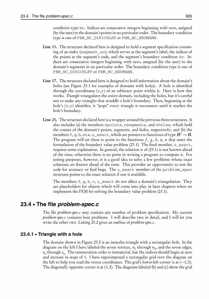
root2014/7/8page 305
�
�
�
�
�
�
�
�
23.4. The file problem-spec.c 305
condition type bc. Indices are consecutive integers beginning with zero, assigned(by the user) to the domain’s points in no particular order. The boundary conditiontype is one of FEM_BC_DIRICHLET or FEM_BC_NEUMANN.
Line 11. The structure declared here is designed to hold a segment specification consist-ing of an index (segment_no), which serves as the segment’s label, the indices ofthe points at the segment’s ends, and the segment’s boundary condition bc. In-dices are consecutive integers beginning with zero, assigned (by the user) to thedomain’s segments in no particular order. The boundary condition type is one ofFEM_BC_DIRICHLET or FEM_BC_NEUMANN.
Line 17. The structure declared here is designed to hold information about the domain’sholes (see Figure 23.1 for examples of domains with holes). A hole is identifiedthrough the coordinates (x, y) of an arbitrary point within it. Here is how thisworks. Triangle triangulates the entire domain, including the holes, but it’s carefulnot to make any triangles that straddle a hole’s boundary. Then, beginning at thehole’s (x, y) identifier, it “pops” every triangle it encounters until it reaches thehole’s boundary.
Line 21. The structure declared here is a wrapper around the previous three structures. Italso includes (a) the members npoints, nsegments, and nholes, which holdthe counts of the domain’s points, segments, and holes, respectively; and (b) themembers f, g, h, eta, u_exact, which are pointers to functions of type R2 →R.The program will set these to point to the functions f , g , h, η, u that enter theformulation of the boundary value problem (23.1). The final member, u_exact,requires some explanation. In general, the solution u of (23.1) is not known aheadof the time; otherwise there is no point in writing a program to compute it. Fortesting purposes, however, it is a good idea to solve a few problems whose exactsolutions are known ahead of the time. This provides an opportunity to test thecode for accuracy or find bugs. The u_exact member of the problem_specstructure points to the exact solution if one is available.
The members f, g, h, c, u_exact do not affect a domain’s triangulation. Theyare placeholders for objects which will come into play in later chapters when weimplement the FEM for solving the boundary value problem (23.1).
23.4 The file problem-spec.cThe file problem-spec.c may contain any number of problem specification. My currentproblem-spec.c contains four problems. I will describe two in detail, and I will let youwrite the other two. Listing 23.2 gives an outline of problem-spec.c.
23.4.1 Triangle with a hole
The domain shown in Figure 23.2 is an isosceles triangle with a rectangular hole. In thediagram on the left I have labeled the seven vertices, n0 through n6, and the seven edges,e0 through e6. The enumeration order is immaterial, but the indices should begin at zeroand increase in steps of 1. I have superimposed a rectangular grid over the diagram onthe left to help you read the vertex coordinates. The grid’s lower-left corner is at (−1,0).The diagonally opposite corner is at (1,2). The diagrams labeled (b) and (c) show the grid

root2014/7/8page 306
�
�
�
�
�
�
�
�
306 Chapter 23. Triangulation with the Triangle library
Listing 23.2: An outline of the file problem-spec.c.
1 � #include ...2 � struct problem_spec *triangle_with_hole(void) ... // see Listing 23.33 � struct problem_spec *annulus(int n) ... // see Listing 23.44 � void free_annulus(struct problem_spec *spec) ... // see Listing 23.55 � struct problem_spec *square(void) ...6 � struct problem_spec *three_holes(int n) ...7 � void free_three_holes(struct problem_spec *spec) ...
n0 n1
n2
e0
e1e2
n3 n4
n5n6
e3
e4
e5
e6
(a) (b) (c)
Figure 23.2: (a) Triangle with a hole before meshing; (b) after meshing with the maxi-mum area parameter set to 0.2; and (c) after meshing with maximum areaparameter set to 0.02. In (a) I have superimposed a rectangular grid to helpyou read the vertex coordinates. The grid’s lower-left corner is at (−1,0).The diagonally opposite corner is at (1,2). The hollow circle at (0,0.75)marks an arbitrary point within the hole. Triangle relies on this to recog-nize the inside of a hole.
generated by the program corresponding to setting the maximum area of triangles to 0.2and 0.02, respectively.
The function triangle_with_hole() that appears on line 2 of Listing 23.2 re-turns a pointer to a problem_spec structure corresponding to the domain in Figure23.2(a). Its implementation is shown in Listing 23.3. Let’s examine the details.
Line 3. We define and initialize the array points[] of the following type:“struct problem_spec_point”. That structure, described in Section 23.3,holds a point’s index, its x and y coordinates, and its boundary condition type.Since our domain has seven vertices/points, the array points[] is of length 7.Lines 5 through 12 define those points.
Thestatic specifier in the declaration of points[]means that the array persiststhroughout the program’s lifetime (that is, from when the program is invoked untilwhen in exits). Thus, a pointer to the structure remains meaningful after the functiontriangle_with_hole() returns. In the absence of the static specifier, thearray would have come into existence upon entering the function and would havevanished upon exiting; therefore the address returned by the function would havebeen meaningless.
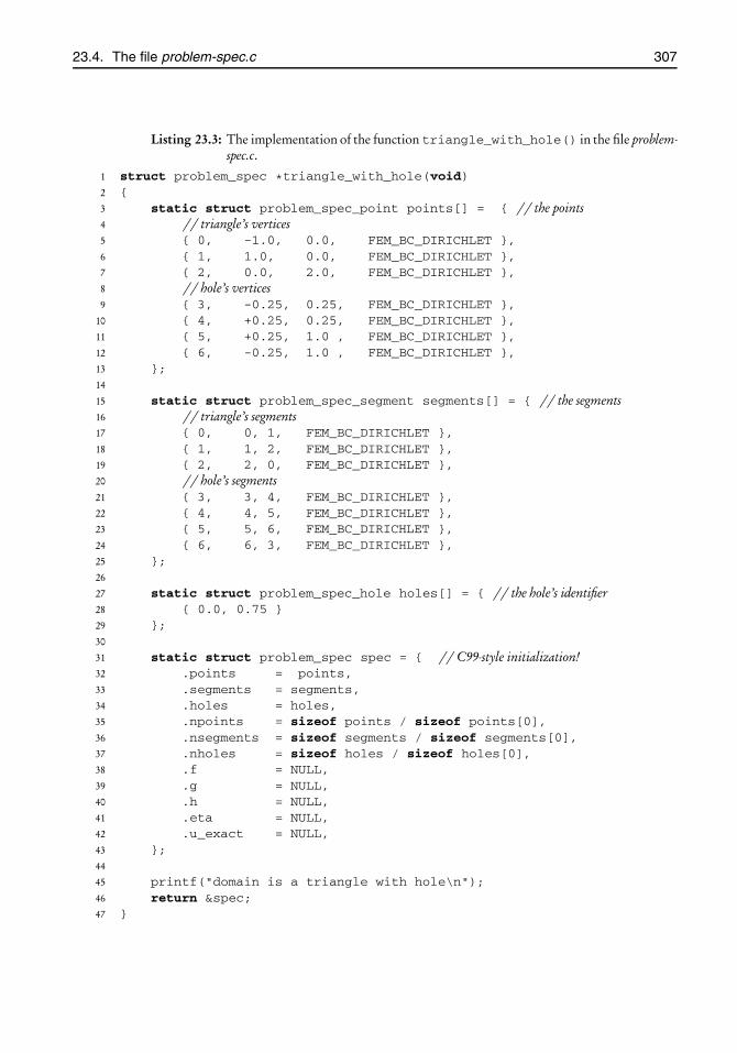
root2014/7/8page 307
�
�
�
�
�
�
�
�
23.4. The file problem-spec.c 307
Listing 23.3: The implementation of the function triangle_with_hole() in the file problem-spec.c.
1 struct problem_spec *triangle_with_hole(void)2 {3 static struct problem_spec_point points[] = { // the points4 // triangle’s vertices5 { 0, -1.0, 0.0, FEM_BC_DIRICHLET },6 { 1, 1.0, 0.0, FEM_BC_DIRICHLET },7 { 2, 0.0, 2.0, FEM_BC_DIRICHLET },8 // hole’s vertices9 { 3, -0.25, 0.25, FEM_BC_DIRICHLET },
10 { 4, +0.25, 0.25, FEM_BC_DIRICHLET },11 { 5, +0.25, 1.0 , FEM_BC_DIRICHLET },12 { 6, -0.25, 1.0 , FEM_BC_DIRICHLET },13 };14
15 static struct problem_spec_segment segments[] = { // the segments16 // triangle’s segments17 { 0, 0, 1, FEM_BC_DIRICHLET },18 { 1, 1, 2, FEM_BC_DIRICHLET },19 { 2, 2, 0, FEM_BC_DIRICHLET },20 // hole’s segments21 { 3, 3, 4, FEM_BC_DIRICHLET },22 { 4, 4, 5, FEM_BC_DIRICHLET },23 { 5, 5, 6, FEM_BC_DIRICHLET },24 { 6, 6, 3, FEM_BC_DIRICHLET },25 };26
27 static struct problem_spec_hole holes[] = { // the hole’s identifier28 { 0.0, 0.75 }29 };30
31 static struct problem_spec spec = { // C99-style initialization!32 .points = points,33 .segments = segments,34 .holes = holes,35 .npoints = sizeof points / sizeof points[0],36 .nsegments = sizeof segments / sizeof segments[0],37 .nholes = sizeof holes / sizeof holes[0],38 .f = NULL,39 .g = NULL,40 .h = NULL,41 .eta = NULL,42 .u_exact = NULL,43 };44
45 printf("domain is a triangle with hole\n");46 return &spec;47 }

root2014/7/8page 308
�
�
�
�
�
�
�
�
308 Chapter 23. Triangulation with the Triangle library
Line 15. We define and initialize the array segments[] of the following type:“struct problem_spec_segment”. That structure, described in Sec-tion 23.3, holds a segment’s index, the indices of the points at its ends, and itsboundary condition type. Since our domain has seven edges/segments, the arraysegments[] is of length 7. Lines 17 through 24 define those segments. The pre-vious paragraph’s comments on the static specifier apply here as well.
Line 27. We define and initialize the array holes[] of the following type:“struct problem_spec_hole”. That structure, described in Section 23.3,holds the x and y coordinates of an arbitrary point inside a hole. Since our do-main has one hole, holes[] is an array of length 1. I have picked (0,0.75) as thishole’s identifier point; see Figure 23.2(a). The previous paragraph’s comments onthe static specifier apply here as well. See the next paragraph regarding domainswith no holes.
Line 31. We define and initialize spec, an object of type “struct problem_spec”,which was described in Section 23.3. Its first three members are the addresses ofthe points[], segments[], and holes[] arrays defined earlier. Its next threemembers are the lengths of those arrays. I could have entered 7, 7, and 1 for thoselengths, but I didn’t. Instead, I let the program itself calculate the lengths followingthe idea noted in Remark 4.2 on page 22. This makes the program more robustbecause if I choose to insert or delete a point in the points[] array, I won’t haveto update the entry here. The rest of the structure’s members are pointers to thevarious functions that enter the definition of the boundary value problem (23.1).These are irrelevant to meshing, so I am setting them to NULL for now.
Remark 23.1. If the domain has no holes, then set.holes toNULL and.nholesto 0.
Line 45. The informational message printed here is by no means essential; however, ithelps make the function a little more user-friendly. Inspect the transcript of theinteractive session in Section 23.2 to see where the message “domain is a trianglewith hole” appears.
23.4.2 An annulus
Figure 23.3 shows an annular domain bounded by two octagons. In the diagram on theleft, I have labeled the domain’s 16 vertices, n0 through n15, and the 16 edges, e0 throughe15. The enumeration order is immaterial, but the indices should begin at zero and in-crease in steps of 1. The distances of the inner points from the center are 0.325. Thedistances of the outer points from the center are twice that. There is no particular reasonfor these choices other than the desire to make the area of the annulus to be approxi-mately 1 so that we may compare its triangulation in a meaningful way to that of a 1× 1square. On the right, I have shown the mesh produced by invoking the program with theargument 0.02.
The function annulus() that appears on line 3 of Listing 23.2 on page 306 returnsa pointer to a problem_spec structure corresponding to the domain in Figure 23.3(a).Its implementation is shown in Listing 23.4. Unlike triangle_with_hole(), whichtakes no arguments, annulus() takes one argument, n, and produces n-gons for theannulus’s inner and outer boundaries. The domain in Figure 23.3 was produced by callingannulus(8).

root2014/7/8page 309
�
�
�
�
�
�
�
�
23.4. The file problem-spec.c 309
n0
n1
n2n3
n4
n5 n6
n7
n8
n9
n10
n11
n12
n13
n14
n15
e0
e1e2
e3
e4
e5 e6
e7
e8
e9e10
e11
e12
e13 e14
e15
(a) (b)
Figure 23.3: (a) An octagonal annulus before meshing; (b) mesh produced byannulus(8) with maximum area parameter set to 0.02. In (a) I haveshown my labeling of the points and segments.
There is a fundamental difference between the functions triangle_with_hole()and annulus(). In the former, the geometry is fixed once for all. I took advantageof that when I combined the declaration and initialization of the points[] array (seeline 3 in Listing 23.3 on page 307). I treated the segments[] and holes[] arrays(Listing 23.3, lines 15 and 27) in the same way. In contrast, the geometry of the annulusis unknown ahead of the time since it depends on the argument n. That prevents us fromcombining the definitions and initializations of the arrays. Instead, we call xmalloc()to allocate arrays of appropriate lengths according to n and then populate their entriesone at a time in for-loops. Additionally, we supply a function, free_annulus(),that the user will call to free the allocated memory when it’s no longer needed. Let usexamine the details.
Line 3. We need the number π to calculate the vertex coordinates. We have tanπ/4= 1,and thereforeπ= 4 tan−1 1. Here we apply the standard library’s atan() functionto evaluate the inverse tangent.
Line 4. We define the annulus’s inner and outer radii a and b . You may change thesenumbers if you wish. Better yet, you may want to modify annulus() so that itreceives a and b as arguments, as in annulus(a,b,n).
The choice of a = 0.325 and b = 2a results in an annulus of area of π(b 2 − a2) ≈0.995. I wanted to get an area close to 1 to compare its triangulation to that of a1× 1 square. There is no deep reason for that choice.
Line 5. Here we declare “spec” as a pointer to “struct problem_spec” and at thesame time allocate memory for the structure.
Lines 6–8. We allocate vectors/arrays to hold the domain’s geometry. The first two vec-tors are of length 2n each because the domain has 2n vertices and 2n edges. Thethird vector is of length 1 because there is only one hole.
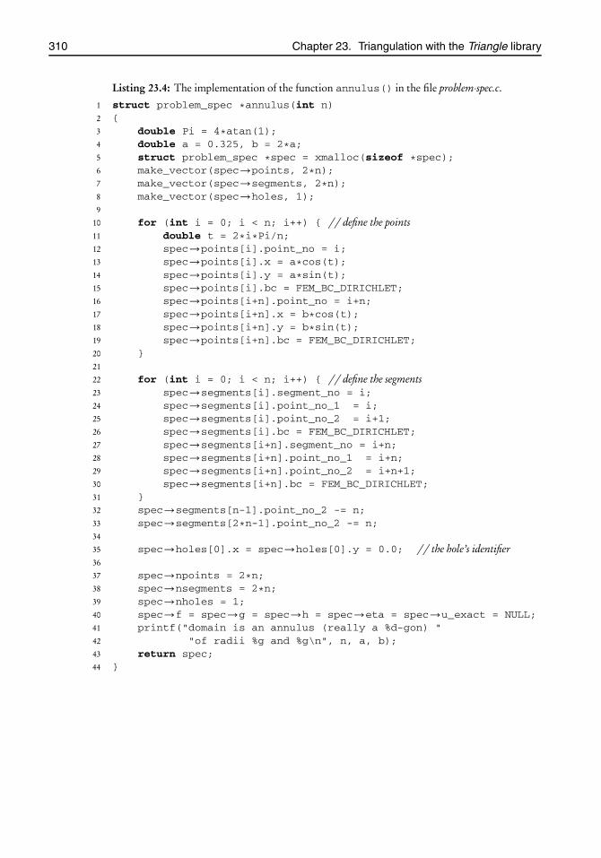
root2014/7/8page 310
�
�
�
�
�
�
�
�
310 Chapter 23. Triangulation with the Triangle library
Listing 23.4: The implementation of the function annulus() in the file problem-spec.c.
1 struct problem_spec *annulus(int n)2 {3 double Pi = 4*atan(1);4 double a = 0.325, b = 2*a;5 struct problem_spec *spec = xmalloc(sizeof *spec);6 make_vector(spec→points, 2*n);7 make_vector(spec→segments, 2*n);8 make_vector(spec→holes, 1);9
10 for (int i = 0; i < n; i++) { // define the points11 double t = 2*i*Pi/n;12 spec→points[i].point_no = i;13 spec→points[i].x = a*cos(t);14 spec→points[i].y = a*sin(t);15 spec→points[i].bc = FEM_BC_DIRICHLET;16 spec→points[i+n].point_no = i+n;17 spec→points[i+n].x = b*cos(t);18 spec→points[i+n].y = b*sin(t);19 spec→points[i+n].bc = FEM_BC_DIRICHLET;20 }21
22 for (int i = 0; i < n; i++) { // define the segments23 spec→segments[i].segment_no = i;24 spec→segments[i].point_no_1 = i;25 spec→segments[i].point_no_2 = i+1;26 spec→segments[i].bc = FEM_BC_DIRICHLET;27 spec→segments[i+n].segment_no = i+n;28 spec→segments[i+n].point_no_1 = i+n;29 spec→segments[i+n].point_no_2 = i+n+1;30 spec→segments[i+n].bc = FEM_BC_DIRICHLET;31 }32 spec→segments[n-1].point_no_2 -= n;33 spec→segments[2*n-1].point_no_2 -= n;34
35 spec→holes[0].x = spec→holes[0].y = 0.0; // the hole’s identifier36
37 spec→npoints = 2*n;38 spec→nsegments = 2*n;39 spec→nholes = 1;40 spec→f = spec→g = spec→h = spec→eta = spec→u_exact = NULL;41 printf("domain is an annulus (really a %d-gon) "42 "of radii %g and %g\n", n, a, b);43 return spec;44 }

root2014/7/8page 311
�
�
�
�
�
�
�
�
23.5. The files mesh.h and mesh.c 311
Listing 23.5: The function free_annulus() in the file problem-spec.c.
1 void free_annulus(struct problem_spec *spec)2 {3 if (spec �= NULL) {4 free_vector(spec→points);5 free_vector(spec→segments);6 free_vector(spec→holes);7 free(spec);8 }9 }
Line 10. In a for-loop we define the vertex coordinates through⎧⎪⎪⎨⎪⎪⎩xi = a cos
2πi
n,
yi = a sin2πi
n,
⎧⎪⎪⎨⎪⎪⎩xn+i = b cos
2πi
n,
yn+i = b sin2πi
n,
i = 0,1, . . . , n− 1.
Thus, the inner vertices are labeled 0 through n − 1, and the outer vertices are la-beled n through 2n− 1. Figure 23.3(a) illustrates the n = 8 case.
Line 22. The for-loop defines the segment i as connecting vertex i to vertex i + 1 fori = 0,1, . . . , 2n − 1. This is not quite correct, however, since the segment n − 1should connect the vertex n − 1 to vertex 0, as the polygon closes onto itself. Thesame problem exists with the segment 2n − 1. We fix these in the two lines thatimmediately follow the for-loop.
Line 35. Here we define the identifier point of the domain’s hole. I have taken the ob-vious choice (0,0), but any other point within the hole, e.g. (a/2,0), would havebeen just as good.
Line 37. We are done with defining the domain’s components. We assign the spec struc-ture’s remaining members, print an informative message, and return spec to thecaller.
This completes the details of the function annulus(). In Listing 23.5 we providea companion function, free_annulus(), to enable the user to free the memory allo-cated within annulus(). The function enters on line 4 of Listing 23.2 on page 306.
23.5 The files mesh.h and mesh.cAt this point we have a framework for specifying a domain’s geometry, such as thatshown in Figure 23.3(a). In this section we introduce a companion framework to addressa domain’s triangulation, such as that seen in Figure 23.3(b).
The data structures for holding the triangulation’s data are declared in the file mesh.hshown in Listing 23.6. Let us examine it.
Line 4. A struct node holds data for a node of the mesh. For the purposes of thisbook, you may think of a node as a triangle’s vertex. In more general FEM appli-cations, nodes may include points other than vertices.

root2014/7/8page 312
�
�
�
�
�
�
�
�
312 Chapter 23. Triangulation with the Triangle library
Listing 23.6: The file mesh.h.
1 #ifndef H_MESH_H2 #define H_MESH_H3 #include "problem-spec.h"4 struct node {5 int nodeno;6 double x;7 double y;8 double z;9 int bc;
10 };11 struct edge {12 int edgeno;13 struct node *n[2]; // pointers to the edge’s endpoints14 int bc;15 };16 struct elem {17 int elemno;18 struct node *n[3]; // pointers to the element’s nodes19 struct edge *e[3]; // pointers to the element’s edges20 double ex[3], ey[3]; // x and y components of the edge vectors21 double area; // element’s area22 };23 struct mesh {24 struct node *nodes; // the array of node structures25 struct edge *edges; // the array of edge structures26 struct elem *elems; // the array of elem structures27 int nnodes;28 int nedges;29 int nelems;30 };31 struct mesh *make_mesh(struct problem_spec *spec, double a);32 void free_mesh(struct mesh *mesh);33 #endif /∗ H_MESH_H */
We see that the node structure has members to hold a node’s index, a boundarycondition type (bc), and the node’s (x, y) coordinates. There is no use for the zmember as far as meshing goes. Later, when we solve PDEs, z will hold the valueof the solution at the point (x, y).
Line 11. A struct edge holds data for an edge of the mesh. An edge is the side ofa triangle. It connects two nodes. The edge structure has members to hold anedge number, a boundary condition type (bc), and an array, n[2], that holds twopointers to the node structures corresponding to the edge’s endpoints.
Line 16. A struct elem holds data for an element of the mesh. I use “element” asa synonym for “triangle” in this context. The element structure has a memberelemno to hold an element’s number; an array n[3] to hold pointers to the nodestructures of the element’s vertices; and an array e[3] to hold pointers to the edgestructures of the element’s edges. Furthermore, the arrays ex[3] and ey[3] holdthe x and y components of the element’s edge vectors, which are depicted in Fig-ure A.1 on page 376. The area member holds the element’s area.
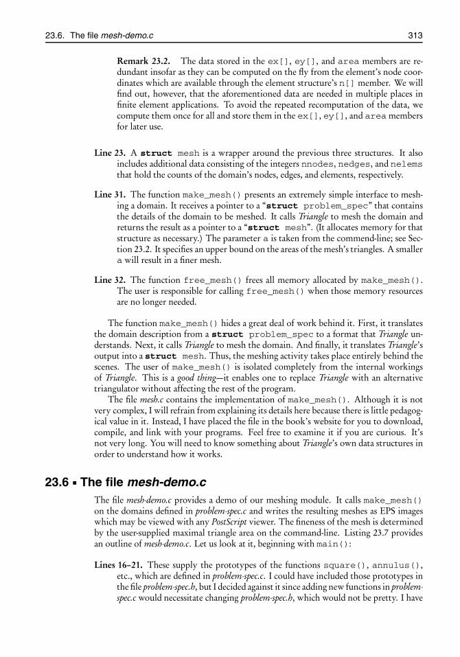
root2014/7/8page 313
�
�
�
�
�
�
�
�
23.6. The file mesh-demo.c 313
Remark 23.2. The data stored in the ex[], ey[], and area members are re-dundant insofar as they can be computed on the fly from the element’s node coor-dinates which are available through the element structure’s n[] member. We willfind out, however, that the aforementioned data are needed in multiple places infinite element applications. To avoid the repeated recomputation of the data, wecompute them once for all and store them in the ex[], ey[], and area membersfor later use.
Line 23. A struct mesh is a wrapper around the previous three structures. It alsoincludes additional data consisting of the integers nnodes, nedges, and nelemsthat hold the counts of the domain’s nodes, edges, and elements, respectively.
Line 31. The function make_mesh() presents an extremely simple interface to mesh-ing a domain. It receives a pointer to a “struct problem_spec” that containsthe details of the domain to be meshed. It calls Triangle to mesh the domain andreturns the result as a pointer to a “struct mesh”. (It allocates memory for thatstructure as necessary.) The parameter a is taken from the commend-line; see Sec-tion 23.2. It specifies an upper bound on the areas of the mesh’s triangles. A smallera will result in a finer mesh.
Line 32. The function free_mesh() frees all memory allocated by make_mesh().The user is responsible for calling free_mesh() when those memory resourcesare no longer needed.
The function make_mesh() hides a great deal of work behind it. First, it translatesthe domain description from a struct problem_spec to a format that Triangle un-derstands. Next, it calls Triangle to mesh the domain. And finally, it translates Triangle’soutput into a struct mesh. Thus, the meshing activity takes place entirely behind thescenes. The user of make_mesh() is isolated completely from the internal workingsof Triangle. This is a good thing—it enables one to replace Triangle with an alternativetriangulator without affecting the rest of the program.
The file mesh.c contains the implementation of make_mesh(). Although it is notvery complex, I will refrain from explaining its details here because there is little pedagog-ical value in it. Instead, I have placed the file in the book’s website for you to download,compile, and link with your programs. Feel free to examine it if you are curious. It’snot very long. You will need to know something about Triangle’s own data structures inorder to understand how it works.
23.6 The file mesh-demo.cThe file mesh-demo.c provides a demo of our meshing module. It calls make_mesh()on the domains defined in problem-spec.c and writes the resulting meshes as EPS imageswhich may be viewed with any PostScript viewer. The fineness of the mesh is determinedby the user-supplied maximal triangle area on the command-line. Listing 23.7 providesan outline of mesh-demo.c. Let us look at it, beginning with main():
Lines 16–21. These supply the prototypes of the functions square(), annulus(),etc., which are defined in problem-spec.c. I could have included those prototypes inthe file problem-spec.h, but I decided against it since adding new functions in problem-spec.c would necessitate changing problem-spec.h, which would not be pretty. I have

root2014/7/8page 314
�
�
�
�
�
�
�
�
314 Chapter 23. Triangulation with the Triangle library
Listing 23.7: An outline of the file mesh-demo.c.
1 � #include ...2 static void do_demo(struct problem_spec *spec,3 double a, char *eps_filename)4 {5 struct mesh *mesh = make_mesh(spec, a);6 printf("vertices = %d, edges = %d, elems = %d\n",7 mesh→nnodes, mesh→nedges, mesh→nelems);8 mesh_to_eps(mesh, eps_filename);9 free_mesh(mesh);
10 }11
12 � static void show_usage(char *progname) ...13
14 int main(int argc, char **argv)15 {16 struct problem_spec *square(void);17 struct problem_spec *triangle_with_hole(void);18 struct problem_spec *annulus(int n);19 void free_annulus(struct problem_spec *spec);20 struct problem_spec *three_holes(int n);21 void free_three_holes(struct problem_spec *spec);22 struct problem_spec *spec;23 char *endptr;24 double a;25
26 � check argc, call show_usage() and exit if other than 227 a = strtod(argv[1], &endptr);28 � check endptr, call show_usage() and exit if bad29
30 do_demo(triangle_with_hole(), a, "triangle-with-hole.eps");31 putchar(’\n’);32
33 spec = annulus(24);34 do_demo(spec, a, "annulus.eps");35 free_annulus(spec);36 putchar(’\n’);37
38 � also do square()39 � also do three_holes()40 return EXIT_SUCCESS;41 }
chosen to include the prototypes in main() since that’s the only place where theyare needed.
Lines 26–28. The program is to be invoked with exactly one argument, a, which spec-ifies the mesh’s maximal triangle area. Therefore, we expect argc to be 2. Weapply the standard library’s strtod() function (see Chapter 5) to extract a. Callshow_usage() and exit if the argument is malformed or if it represents a non-positive number.
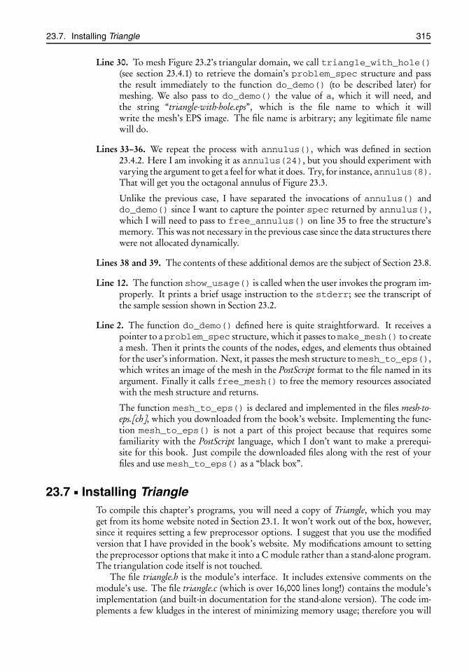
root2014/7/8page 315
�
�
�
�
�
�
�
�
23.7. Installing Triangle 315
Line 30. To mesh Figure 23.2’s triangular domain, we call triangle_with_hole()(see section 23.4.1) to retrieve the domain’s problem_spec structure and passthe result immediately to the function do_demo() (to be described later) formeshing. We also pass to do_demo() the value of a, which it will need, andthe string “triangle-with-hole.eps”, which is the file name to which it willwrite the mesh’s EPS image. The file name is arbitrary; any legitimate file namewill do.
Lines 33–36. We repeat the process with annulus(), which was defined in section23.4.2. Here I am invoking it as annulus(24), but you should experiment withvarying the argument to get a feel for what it does. Try, for instance, annulus(8).That will get you the octagonal annulus of Figure 23.3.
Unlike the previous case, I have separated the invocations of annulus() anddo_demo() since I want to capture the pointer spec returned by annulus(),which I will need to pass to free_annulus() on line 35 to free the structure’smemory. This was not necessary in the previous case since the data structures therewere not allocated dynamically.
Lines 38 and 39. The contents of these additional demos are the subject of Section 23.8.
Line 12. The function show_usage() is called when the user invokes the program im-properly. It prints a brief usage instruction to the stderr; see the transcript ofthe sample session shown in Section 23.2.
Line 2. The function do_demo() defined here is quite straightforward. It receives apointer to a problem_spec structure, which it passes tomake_mesh() to createa mesh. Then it prints the counts of the nodes, edges, and elements thus obtainedfor the user’s information. Next, it passes the mesh structure to mesh_to_eps(),which writes an image of the mesh in the PostScript format to the file named in itsargument. Finally it calls free_mesh() to free the memory resources associatedwith the mesh structure and returns.
The function mesh_to_eps() is declared and implemented in the files mesh-to-eps.[ch], which you downloaded from the book’s website. Implementing the func-tion mesh_to_eps() is not a part of this project because that requires somefamiliarity with the PostScript language, which I don’t want to make a prerequi-site for this book. Just compile the downloaded files along with the rest of yourfiles and use mesh_to_eps() as a “black box”.
23.7 Installing TriangleTo compile this chapter’s programs, you will need a copy of Triangle, which you mayget from its home website noted in Section 23.1. It won’t work out of the box, however,since it requires setting a few preprocessor options. I suggest that you use the modifiedversion that I have provided in the book’s website. My modifications amount to settingthe preprocessor options that make it into a C module rather than a stand-alone program.The triangulation code itself is not touched.
The file triangle.h is the module’s interface. It includes extensive comments on themodule’s use. The file triangle.c (which is over 16,000 lines long!) contains the module’simplementation (and built-in documentation for the stand-alone version). The code im-plements a few kludges in the interest of minimizing memory usage; therefore you will

root2014/7/8page 316
�
�
�
�
�
�
�
�
316 Chapter 23. Triangulation with the Triangle library
get warnings when you compile it with gcc’s -Wall -pedantic flags. Nevertheless,the compiled program seems to work on the machines I have tested.
You may drop the files triangle.h and triangle.c into your project’s directory and treatthem like any *.c and *.h file of your own. Although that will work, it’s not a good idea.First, mixing triangle.h and triangle.c with your own files is ugly. Second, triangle.h andtriangle.c are needed in several other projects. It makes no sense to keep multiple copiesof them. Third, triangle.c is quite large and it takes several seconds to compile even on afast machine. It will slow you down if you have to compile it often.
To address these issues, I suggest that you put triangle.h and triangle.c in a directoryof their own, let’s say ../triangle/, relative to your current project’s directory. Go to thatdirectory, and compile Triangle once for all:
$ cd ../triangle/$ cc -Wall -pedantic -std=c89 -O2 triangle.c -c
This will produce the object file triangle.o. There will be several warnings due to thekludges noted above. Ignore the warnings.
Now go to your project’s directory and establish symbolic links to Triangle:
$ cd ../meshing/$ ln -s ../triangle/triangle.[ho] .
(Don’t overlook the space and the period at the end of that command.) This makes thefiles triangle.h and triangle.o available to your project. Compile and link with the rest ofyour project’s files as usual.
Remark 23.3. If you know how to make libraries on your operating system, youmay build a true library out of triangle.o and install it, along with triangle.h, in stan-dard places where the compiler looks for libraries and header files. Then you may linkyour program with Triangle simply by giving a -ltriangle flag to the compiler at thelinking stage. There are too many variations and platform dependencies on making andinstalling libraries; therefore I cannot afford to go into that subject in any depth. If youdon’t know how, ask someone versed in the use of your platform to show you.
23.8 Project TriangulateListing 23.2 on page 306 gives an outline of the file problem-spec.c. Some of its parts havebeen explained in the preceding sections. Complete the rest of that file according to theinstructions below.
Part 23.1. The function square() in Listing 23.2 defines a domain in the form of asimple square (0,1)× (0,1).
1. Add the definition of square() to problem-spec.c.2. Insert the necessary code in mesh-demo.c (see line 38 of Listing 23.7) that calls
do_demo() to mesh the domain. A sample result is shown in Figure 23.1 onpage 302.
Part 23.2. The function three_holes() in Listing 23.2 defines an L-shaped domainwith three holes removed, as shown in Figure 23.1 on page 302. Each hole is an n-gon,where n is received as an argument.

root2014/7/8page 317
�
�
�
�
�
�
�
�
23.8. Project Triangulate 317
1. Add the definition of three_holes() to problem-spec.c.2. Insert the necessary code in mesh-demo.c (see line 39 of Listing 23.7) that calls
do_demo() to mesh the domain.
Suggestion: Set the domain’s reentrant vertex at (0,0) and the other vertices at (s , 0), (s , s),(−s , s), (−s ,−s), and (0,−s). Let r = s/4 be the hole radius. You may pick any numberyou wish for s . I used s = 0.64 because that makes the domain’s area approximately equalto 1.
root2014/7/8page 319
�
�
�
�
�
�
�
�
Chapter 24
Integration on triangles
Prerequisites: Chapters 7, 8, 23, and Appendix A
24.1 IntroductionThe Gaussian quadrature algorithm of Chapter 22 gives the optimal distribution of quadra-ture points and weights for integrating numerically a function of one variable on an inter-val. It identifies the points and weights as simple functions of the roots of certain Legendrepolynomials.
Unfortunately no such definitive procedure exists for integrating a function of twovariables over a triangle. True, one may regard the triangle as the image of a square,and the square as the product of two intervals, and thus extend the Gaussian quadratureto a triangle. However, the distribution of the quadrature points obtained this way isfar from optimal, as evidenced by the illustration in Figure 24.1; the quadrature pointscrowd into one vertex, requiring many essentially redundant function evaluations there.An efficient quadrature scheme will distribute the quadrature points more evenly on thetriangle. The purpose of this chapter is to introduce one such quadrature scheme that hasbeen developed by Taylor, Wingate, and Bos [75, 74].
An n-point quadrature rule on a triangle T selects n points,(xi , yi )
-ni=1, and weights
{wi}ni=1, so that for all reasonably nice functions f (x, y) defined on T one has
∫T
f (x, y)d x d y ≈n∑
i=1
wi f (xi , yi ).
Cartesian coordinates, however, do not mesh well with triangles. Barycentric coordi-nates (see Appendix A) work much better, and that’s what we will use most of time whendealing with triangles.
A point inside a triangle may be expressed in Cartesian coordinates (x, y) or barycen-tric coordinates (λ1,λ2,λ3), where 0 ≤ λ1,λ2,λ3 ≤ 1 and λ1 + λ2 + λ3 = 1. There is aone-to-one correspondence between the Cartesian and barycentric coordinates. There-fore, to a function f (x, y) expressed in Cartesian coordinates there corresponds a func-tion f (λ1,λ2,λ3) in barycentric coordinates so that f (x, y) = f (λ1,λ2,λ3), where (x, y)and (λ1,λ2,λ3) refer to the same point. The n-point quadrature formula shown above
319

root2014/7/8page 320
�
�
�
�
�
�
�
�
320 Chapter 24. Integration on triangles
ξ
η
x
y�
x = (1−η)ξ /2y = η
Figure 24.1: The diagram shows a mapping of the square (−1,1)× (−1,1) in the (ξ ,η)plane to a triangle in the (x, y) plane. The (4× 4)-point Gaussian quadra-ture on the square maps to a certain quadrature scheme on the triangle.The distribution of the triangle’s quadrature points, however, is far fromoptimal—they crowd into one vertex.
may be expressed in the equivalent form∫T
f (x, y)d x d y ≈n∑
i=1
wi f�λ(i )1 ,λ(i )2 ,λ(i )3
,
where�λ(i )1 ,λ(i )2 ,λ(i )3
are the barycentric coordinates of the quadrature points.
The benefit of formulating the quadrature in terms of the barycentric coordinates isthat once we determine a good set of quadrature points on one triangle—any triangle willdo—the result extends to all triangles. This is because any triangle may be mapped ontoany another through a linear transformation, and barycentric coordinates are invariantunder linear mappings (subsection A.1.2).
The quadrature weights, however, are proportional to the triangle’s area since theJacobian determinant of a linear transformation is constant and measures the ratio of theareas. The usual practice is to tabulate the weights corresponding to a standard referencetriangle, let’s call it Tstd, and then adjust the quadrature formula for arbitrary triangles bymultiplying by the area ratios. This leads to the quadrature formula∫
Tf (x, y)d x d y ≈ |T |
|Tstd|n∑
i=1
wi f�λ(i )1 ,λ(i )2 ,λ(i )3
, (24.1)
where |T | and |Tstd| are the areas of the triangle T and the standard reference triangle Tstd.Generally a larger n gives a better approximation. The optimal placement of the
quadrature points and their weights depends on n.87 The coarsest approximation is ob-tained with n = 1, which calls for sampling the function in just one point to estimate thevalue of the integral. How good is the formula (24.1) if we pick the sampling point, thatis,�λ(1)1 ,λ(1)2 ,λ(1)3
, arbitrarily in T and take w1 = |Tstd|? Certainly not very good but not
entirely useless either. For instance, it will give exact results for constant functions. (Doyou see that?) We can do even better. If we sample the function at the triangle’s centroid,then it is not hard to see that (24.1) with n = 1 will give exact results not only for con-stants but also for all first degree polynomials! In that sense, the choice of the quadraturepoint (λ1,λ2,λ3) = (1/3,1/3,1/3), which picks up the centroid, and the weight w = |Tstd|is optimal for a one-point quadrature.
87In that regard I should have written�λ(n,i )
1 ,λ(n,i )2 ,λ(n,i )
3
and w (n)i to make the dependence on n explicit, but
I didn’t want to complicate the notation.

root2014/7/8page 321
�
�
�
�
�
�
�
�
24.2. The Taylor, Wingate, and Bos (TWB) quadrature 321
This brings up a question: What is the smallest number of quadrature points, n, forwhich the formula (24.1) gives exact answers for all quadratic polynomials? There is noreason to stop at quadratics. We may ask the question of polynomials of any degree. Forinstance, what is the smallest number of quadrature points, n, for which the formula (24.1)gives exact answers for all polynomials of degree 14?
A general answer to such questions is not known. There are various algorithms forcomputing n and the corresponding points and weights, but there is no assurance thatthey actually are optimal. For instance, according to Table 2 of [74], three different algo-rithms in [13], [78], and [74] for exact quadrature of polynomials of degree 14 call for 42,46, and 45 points, respectively. It is not known if 42 points is the fewest possible.
The goal of this chapter is to learn how to integrate on triangles with the help of thequadrature data developed by Taylor, Wingate, and Bos [75, 74]. Unlike most other chap-ters of this book, this chapter’s study does not lead to a self-contained module. The reasonis that in applications such as finite element models, integrations take place at the inner-most level of multiply nested loops. It is significantly more efficient to insert a customizedintegration code directly in the heart of the nested loops rather than pass data back andforth to a general external module to evaluate the integrals. Consequently, we will usethis chapter’s ideas and techniques, rather than its C code, in future chapters.
24.2 The Taylor, Wingate, and Bos (TWB) quadratureThe article [74] describes the algorithm used by Taylor, Wingate, and Bos to determinequadrature data (i.e., points and weights) for integration over triangles. The raw data isavailable for electronic downloading from arXiv.org ; see [75]. The same data, wrappedinto a C program, is available at this book’s website as files twb-quad.[ch]. In this sectionI will describe the organization of the data in those files and explain how to use themin computations. I call the resulting procedure TWB quadrature after the initials of theauthors. Before we go on, I must add that there are other data sets for quadrature ontriangles. Lyness and Cools [42] provide a survey of the available methods at the time ofits publication in 1994. This was updated later in Cools [13]. Wandzura and Xiao [78]provide an alternative set of quadrature tables. The article by Xiao and Gimbutas [82]generalizes the technique to higher-dimensional domains. Also see the references in [74].My choice of the TWB quadrature for the purposes of this book is mostly due to the easyavailability of their data.
The TWB quadrature data consists of 14 tables, each corresponding to a certain quadra-ture strength. A quadrature table is said to have a strength of d if it produces exact answersfor all polynomials of degree less than or equal to d . The “exact answer” should be quali-fied, however, since it is subject to the computer’s floating point roundoff errors, as wellas the numerical precision of the tables themselves. The order of magnitude of the relativeerror in a TWB quadrature is roughly around 10−14. Table 5.1 of [75] gives more detailederror estimates.
Table 24.1 lists the quadrature strengths, d , and the corresponding number of quadra-ture points, n, of the 14 TWB quadrature tables. Thus, for instance, a polynomial ofdegree 5 may be integrated exactly through a 10-point TWB quadrature. Table 24.2 liststhat quadrature’s 10 coordinates and weights. For each quadrature point it gives two ofthe three barycentric coordinates (λ1,λ2,λ3). The third may be computed from λ1+λ2+λ3 = 1. The weights add up to 2, indicating that the area of the standard reference trian-gle, |Tstd|, is 2. Integrating a function over a triangle is a matter of plugging the numbersfrom that table into the formula (24.1). Figure 24.2 shows the distribution of the TWBquadrature points corresponding to strengths d = 5 and d = 11.
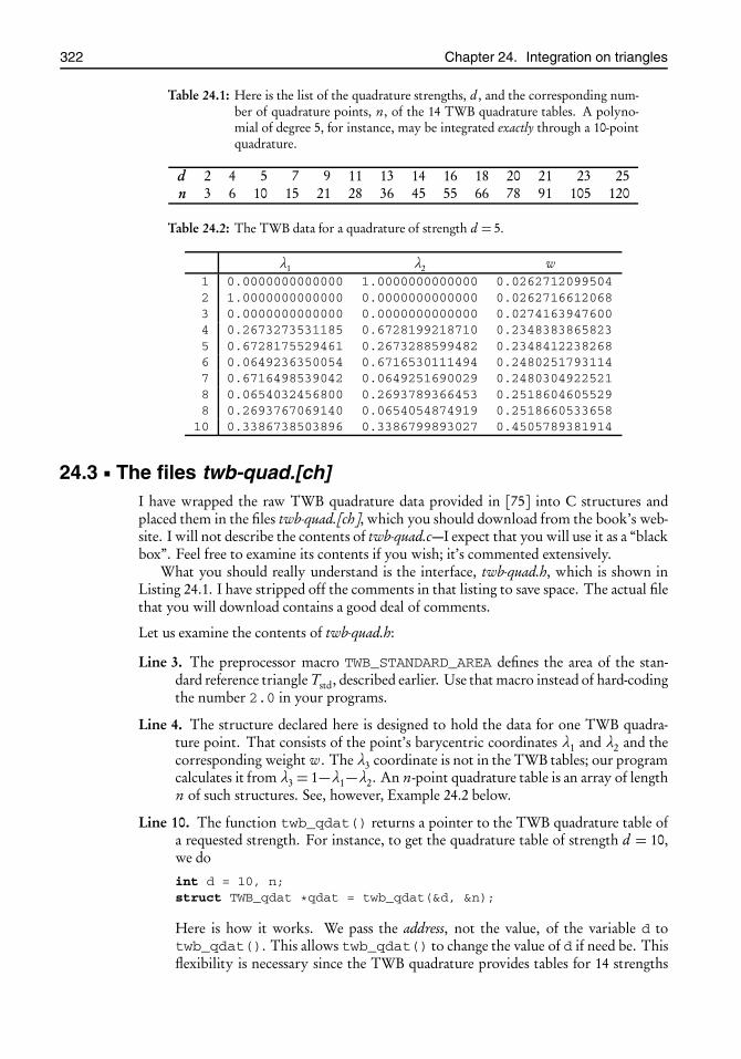
root2014/7/8page 322
�
�
�
�
�
�
�
�
322 Chapter 24. Integration on triangles
Table 24.1: Here is the list of the quadrature strengths, d , and the corresponding num-ber of quadrature points, n, of the 14 TWB quadrature tables. A polyno-mial of degree 5, for instance, may be integrated exactly through a 10-pointquadrature.
d 2 4 5 7 9 11 13 14 16 18 20 21 23 25n 3 6 10 15 21 28 36 45 55 66 78 91 105 120
Table 24.2: The TWB data for a quadrature of strength d = 5.
λ1 λ2 w1 0.0000000000000 1.0000000000000 0.02627120995042 1.0000000000000 0.0000000000000 0.02627166120683 0.0000000000000 0.0000000000000 0.02741639476004 0.2673273531185 0.6728199218710 0.23483838658235 0.6728175529461 0.2673288599482 0.23484122382686 0.0649236350054 0.6716530111494 0.24802517931147 0.6716498539042 0.0649251690029 0.24803049225218 0.0654032456800 0.2693789366453 0.25186046055298 0.2693767069140 0.0654054874919 0.251866053365810 0.3386738503896 0.3386799893027 0.4505789381914
24.3 The files twb-quad.[ch]I have wrapped the raw TWB quadrature data provided in [75] into C structures andplaced them in the files twb-quad.[ch], which you should download from the book’s web-site. I will not describe the contents of twb-quad.c—I expect that you will use it as a “blackbox”. Feel free to examine its contents if you wish; it’s commented extensively.
What you should really understand is the interface, twb-quad.h, which is shown inListing 24.1. I have stripped off the comments in that listing to save space. The actual filethat you will download contains a good deal of comments.
Let us examine the contents of twb-quad.h:
Line 3. The preprocessor macro TWB_STANDARD_AREA defines the area of the stan-dard reference triangle Tstd, described earlier. Use that macro instead of hard-codingthe number 2.0 in your programs.
Line 4. The structure declared here is designed to hold the data for one TWB quadra-ture point. That consists of the point’s barycentric coordinates λ1 and λ2 and thecorresponding weight w. The λ3 coordinate is not in the TWB tables; our programcalculates it from λ3 = 1−λ1−λ2. An n-point quadrature table is an array of lengthn of such structures. See, however, Example 24.2 below.
Line 10. The function twb_qdat() returns a pointer to the TWB quadrature table ofa requested strength. For instance, to get the quadrature table of strength d = 10,we do
int d = 10, n;struct TWB_qdat *qdat = twb_qdat(&d, &n);
Here is how it works. We pass the address, not the value, of the variable d totwb_qdat(). This allows twb_qdat() to change the value of d if need be. Thisflexibility is necessary since the TWB quadrature provides tables for 14 strengths
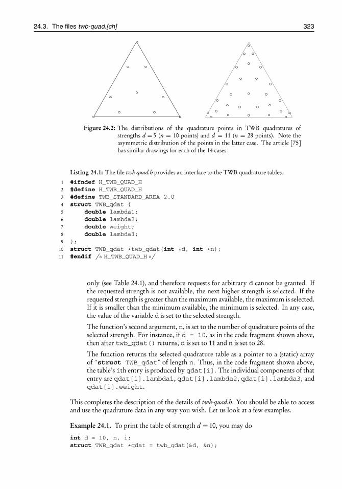
root2014/7/8page 323
�
�
�
�
�
�
�
�
24.3. The files twb-quad.[ch] 323
Figure 24.2: The distributions of the quadrature points in TWB quadratures ofstrengths d = 5 (n = 10 points) and d = 11 (n = 28 points). Note theasymmetric distribution of the points in the latter case. The article [75]has similar drawings for each of the 14 cases.
Listing 24.1: The file twb-quad.h provides an interface to the TWB quadrature tables.
1 #ifndef H_TWB_QUAD_H2 #define H_TWB_QUAD_H3 #define TWB_STANDARD_AREA 2.04 struct TWB_qdat {5 double lambda1;6 double lambda2;7 double weight;8 double lambda3;9 };
10 struct TWB_qdat *twb_qdat(int *d, int *n);11 #endif /∗ H_TWB_QUAD_H ∗/
only (see Table 24.1), and therefore requests for arbitrary d cannot be granted. Ifthe requested strength is not available, the next higher strength is selected. If therequested strength is greater than the maximum available, the maximum is selected.If it is smaller than the minimum available, the minimum is selected. In any case,the value of the variable d is set to the selected strength.
The function’s second argument, n, is set to the number of quadrature points of theselected strength. For instance, if d = 10, as in the code fragment shown above,then after twb_qdat() returns, d is set to 11 and n is set to 28.
The function returns the selected quadrature table as a pointer to a (static) arrayof “struct TWB_qdat” of length n. Thus, in the code fragment shown above,the table’s ith entry is produced by qdat[i]. The individual components of thatentry are qdat[i].lambda1, qdat[i].lambda2, qdat[i].lambda3, andqdat[i].weight.
This completes the description of the details of twb-quad.h. You should be able to accessand use the quadrature data in any way you wish. Let us look at a few examples.
Example 24.1. To print the table of strength d = 10, you may do
int d = 10, n, i;struct TWB_qdat *qdat = twb_qdat(&d, &n);
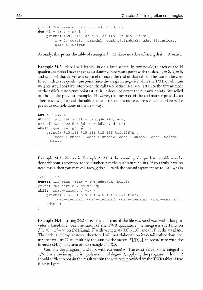
root2014/7/8page 324
�
�
�
�
�
�
�
�
324 Chapter 24. Integration on triangles
printf("we have d = %d, n = %d\n", d, n);for (i = 0; i < n; i++)
printf("%3d: %15.12f %15.12f %15.12f %15.12f\n",i + 1, qdat[i].lambda1, qdat[i].lambda2, qdat[i].lambda3,qdat[i].weight);
Actually, this prints the table of strength d = 11 since no table of strength d = 10 exists.
Example 24.2. Here I will let you in on a little secret. In twb-quad.c, to each of the 14quadrature tables I have appended a dummy quadrature point with the dataλ1 = 0, λ2 = 0,and w = −1 that serves as a sentinel to mark the end of that table. This cannot be con-fused with a true quadrature point since the weight is negative while the TWB quadratureweights are all positive. Moreover, the calltwb_qdat(&d,&n) sets n to the true numberof the table’s quadrature points (that is, it does not count the dummy point). We reliedon that in the previous example. However, the presence of the end-marker provides analternative way to read the table that can result in a more expressive code. Here is theprevious example done in the new way:
int d = 10, n;struct TWB_qdat *qdat = twb_qdat(&d, &n);printf("we have d = %d, n = %d\n", d, n);while (qdat→weight �= -1) {
printf("%15.12f %15.12f %15.12f %15.12f\n",qdat→lambda1, qdat→lambda2, qdat→lambda3, qdat→weight);
qdat++;}
Example 24.3. We saw in Example 24.2 that the scanning of a quadrature table may bedone without a reference to the number n of the quadrature points. If you truly have noneed for n, then you may call twb_qdat() with the second argument set to NULL, as in
int d = 10;struct TWB_qdat *qdat = twb_qdat(&d, NULL);printf("we have d = %d\n", d);while (qdat→weight �= -1) {
printf("%15.12f %15.12f %15.12f %15.12f\n",qdat→lambda1, qdat→lambda2, qdat→lambda3, qdat→weight);
qdat++;}
Example 24.4. Listing 24.2 shows the contents of the file twb-quad-minimal.c that pro-vides a bare-bones demonstration of the TWB quadrature. It integrates the functionf (x, y) = x2+ y2 on the triangle T with vertices at (0,0), (1,0), and (0,1) in the xy plane.The code is self-explanatory; therefore I will not elaborate on its details other than not-ing that on line 27 we multiply the sum by the factor |T |/|Tstd|, in accordance with theformula (24.1). The area of our triangle T is 0.5.
Compile the program, and link with twb-quad.o. The exact value of the integral is1/6. Since the integrand is a polynomial of degree 2, applying the program with d = 2should suffice to obtain the result within the accuracy provided by the TWB tables. Hereis what I get:
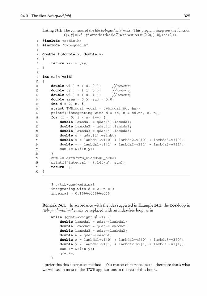
root2014/7/8page 325
�
�
�
�
�
�
�
�
24.3. The files twb-quad.[ch] 325
Listing 24.2: The contents of the file twb-quad-minimal.c. This program integrates the functionf (x, y) = x2+ y2 over the triangle T with vertices at (0,0), (1,0), and (0,1).
1 #include <stdio.h>2 #include "twb-quad.h"3
4 double f(double x, double y)5 {6 return x*x + y*y;7 }8
9 int main(void)10 {11 double v1[] = { 0, 0 }; // vertex v112 double v2[] = { 1, 0 }; // vertex v213 double v3[] = { 0, 1 }; // vertex v314 double area = 0.5, sum = 0.0;15 int d = 2, n, i;16 struct TWB_qdat *qdat = twb_qdat(&d, &n);17 printf("integrating with d = %d, n = %d\n", d, n);18 for (i = 0; i < n; i++) {19 double lambda1 = qdat[i].lambda1;20 double lambda2 = qdat[i].lambda2;21 double lambda3 = qdat[i].lambda3;22 double w = qdat[i].weight;23 double x = lambda1*v1[0] + lambda2*v2[0] + lambda3*v3[0];24 double y = lambda1*v1[1] + lambda2*v2[1] + lambda3*v3[1];25 sum += w*f(x,y);26 }27 sum *= area/TWB_STANDARD_AREA;28 printf("integral = %.14f\n", sum);29 return 0;30 }
$ ./twb-quad-minimalintegrating with d = 2, n = 3integral = 0.16666666666666
Remark 24.1. In accordance with the idea suggested in Example 24.2, the for-loop intwb-quad-minimal.c may be replaced with an index-free loop, as in
while (qdat→weight �= -1) {double lambda1 = qdat→lambda1;double lambda2 = qdat→lambda2;double lambda3 = qdat→lambda3;double w = qdat→weight;double x = lambda1*v1[0] + lambda2*v2[0] + lambda3*v3[0];double y = lambda1*v1[1] + lambda2*v2[1] + lambda3*v3[1];sum += w*f(x,y);qdat++;
}
I prefer this this alternative method—it’s a matter of personal taste—therefore that’s whatwe will see in most of the TWB applications in the rest of this book.

root2014/7/8page 326
�
�
�
�
�
�
�
�
326 Chapter 24. Integration on triangles
Listing 24.3: The transcript of an interactive session with the program twb-quad-demo.
1 $ ./twb-quad-demo2 Usage: ./twb-quad-demo d a3 d = the TWB quadrature strength4 a = maximal triangle area5
6 $ ./twb-quad-demo 4 0.017 quadrature strength = 4, number of points = 68
9 domain is a triangle with hole10 vertices = 158, edges = 408, elems = 25011 geomview output written to file triangle_with_hole.gv12 integral = -0.06857204861110513
14 domain is an annulus (really a 12-gon) of radii 0.325 and 0.6515 vertices = 94, edges = 246, elems = 15216 geomview output written to file annulus.gv17 integral = -2.9553796953088e-1018
19 domain is a square20 vertices = 96, edges = 254, elems = 15921 geomview output written to file square.gv22 integral = 0.999999999999923
24 domain is an L-shape with three holes (actually 12-gons25 vertices = 112, edges = 274, elems = 16026 geomview output written to file three_holes.gv27 integral = 0.28554098238704
24.4 The programWith the help of the triangulation tools developed in Chapter 23, we are now in a posi-tion to integrate a function on any polygonal domain. It’s a matter of triangulating thedomain, integrating over the individual triangles, and adding the results. This capabilityis of utmost importance—integrating over arbitrary polygonal domains is at the heart ofthe FEM, as we will see in Chapter 25.
In this chapter’s Projects section we write a program to compute∫∫Ω
f (x, y)d x d y forvarious functions f over the domains Ω that we worked with in Chapter 23. As noted inSection 24.1, we are not going to encapsulate this chapter’s work in a module since we willfind it more practical to apply the ideas and techniques, rather than the programs, that wewill develop here. Listing 24.3 is the transcript of an interactive session with this chapter’sprogram.
As we see, the program is invoked as “./twb-quad-demo 4 0.01”. It integratesfour functions over the domains triangle_with_hole, annulus, square, and three_holes, whichwere introduced in Chapter 23, by triangulating the domains with a maximal area param-eter of 0.01 and integrating over each triangle with a quadrature strength of 4. The inte-grands vary from case to case—they are specified in problem-spec.c. The integration oversquare computes ∫ 1
0
∫ 1
036xy(1− x)(1− y)d x d y.
root2014/7/8page 327
�
�
�
�
�
�
�
�
24.4. The program 327
The exact value is 1, as it’s trivial to evaluate that integral by hand. The program produces0.9999999999999, which is within the floating point accuracy of the quadrature tables. Anaccurate outcome is expected since the integrand is a polynomial of degree 4 and we areapplying a quadrature of strength 4.
The integration over triangle_with_hole computes∫∫Ω
2
5xy(2− x)(2− y)d x d x.
The exact answer −15799/230400 ≈ −0.068572048611111 . . . . Again, we see that thevalue computed by the program is within the floating point accuracy of the quadraturetables.
The integration over annulus computes∫∫Ω
1
5cos
*3 tan−1 y
x
+d x d y,
which is equivalent to integrating 15 cos 3t in polar coordinates. The integral’s exact value
is zero due to the symmetries of the domain and the integrand; however, we don’t expectan exact quadrature since (a) the function being integrated is not a polynomial, and (b) thedomain is bounded by polygons rather than true circles. Nonetheless, the computed resultis quite respectably close to zero, albeit as a result of cancellations due to symmetries ratherthan a precise quadrature.
The integrand in the case of three_holes is f (x, y) = x2 + y2. You may change that ifyou wish.
Listing 24.4 shows the transcript of a sequence of additional experiments on squareand the same fourth degree polynomial as before. I have set the maximal area parameterto 1. This produces the coarsest possible triangular mesh—two triangles only. In the threeexperiments shown, I reduce the quadrature strength from 4 to 3 to 2.
The result of the experiment on lines 1–6 is within 10−14 of the exact answer, as itshould be, since we are integrating a fourth degree polynomial with quadrature of strengthd = 4.
At first sight the outcome of the experiment on lines 8–13 seems unexpected sincethe answer remains unchanged despite the reduction in the quadrature strength. A closerlook reveals, however—see line 9—that the program is applying a quadrature strength of 4despite the request for a strength of 3. Why? See the list of the 14 available strengths inTable 24.1. There is no table of strength d = 3. The program detects that and picks up thenext higher strength, which is d = 4.
On the other hand, the request for a quadrature strength of d = 2 on line 15 meetsthe program’s approval and it duly produces the answer 0.9722, which shows a signifi-cant deterioration of accuracy, as may be expected since we are applying a quadrature ofstrength 2 to integrate a polynomial of degree 4.
24.4.1 Program files
In addition to the files twb-quad.[ch] discussed earlier, the implementation of the programdepends on the files xmalloc.[ch] from Chapter 7, the file array.h from Chapter 8, and thefiles mesh.[ch] from Chapter 23. Furthermore, you will need a copy (not a link since we aregoing to modify it) of the file problem-spec.c from Chapter 23. The file problem-spec.h is notgoing to change; therefore a symbolic link is fine. Therefore, following the suggestions in

root2014/7/8page 328
�
�
�
�
�
�
�
�
328 Chapter 24. Integration on triangles
Listing 24.4: The transcript of a second interactive session with the program twb-quad-demo. Wereduce the quadrature strength from 4 to 3 to 2. The mesh consists of two trianglesonly.
1 ./twb-quad-demo 4 12 quadrature strength = 4, number of points = 63 domain is a square4 vertices = 4, edges = 5, elems = 25 geomview output written to file square.gv6 integral = 0.9999999999998317
8 ./twb-quad-demo 3 19 quadrature strength = 4, number of points = 6
10 domain is a square11 vertices = 4, edges = 5, elems = 212 geomview output written to file square.gv13 integral = 0.99999999999983114
15 ./twb-quad-demo 2 116 quadrature strength = 2, number of points = 317 domain is a square18 vertices = 4, edges = 5, elems = 219 geomview output written to file square.gv20 integral = 0.972222222222193
Chapters 2 and 6, your project’s directory initially will look like this:88
$ cd twb-quad$ ls -FMakefile plot-with-geomview.c triangle.h@ twb-quad.carray.h@ plot-with-geomview.h triangle.o@ twb-quad.hmesh.c@ problem-spec.c twb-quad-demo.c [email protected]@ problem-spec.h@ twb-quad-minimal.c xmalloc.h@
We saw the purpose and contents of twb-quad-minimal.c in Example 24.4 on page 324. Inthe following sections I will describe the contents of the files plot-with-geomview.[ch] andtwb-quad-demo.c and delineate the required changes to problem-spec.c.
24.5 The files plot-with-geomview.[ch]The integral of a function over a domain is just a number, and that’s what we expect anintegration program to produce. Our program, however, does more. In addition to pro-ducing the numerical value of the integral, it also writes a file—a Geomview script, to beprecise—which may be fed to Geomview (see page 8) to plot a graph of the integrand as asurface in the three-dimensional space. The graphs in Figure 24.3 (page 335) are screen-shots of Geomview’s display.
For the purposes of this chapter, plotting graphs is a mere frill and certainly not centralto evaluating integrals. We do it to satisfy our curiosity regarding the shape of the domain
88Just as in Chapter 23, the files triangle.[ho] link to where you keep your Triangle files. If you have installedTriangle as a library, then these are not needed; just link your program with the -ltriangle flag instead. SeeSection 23.7 for more on this subject.

root2014/7/8page 329
�
�
�
�
�
�
�
�
24.6. Modifying the file problem-spec.c 329
Listing 24.5: The file plot-with-geomview.h provides the interface to a module for writing Ge-omview scripts to visualize three-dimensional graphs of function defined on a mesh.
1 #ifndef H_PLOT_WITH_GEOMVIEW_H2 #define H_PLOT_WITH_GEOMVIEW_H3 #include "mesh.h"4 void plot_with_geomview_mono(struct mesh *mesh, char *filename);5 void plot_with_geomview_zhue(struct mesh *mesh, char *filename);6 #endif /∗ H_PLOT_WITH_GEOMVIEW_H */
and the integrand’s graph. If you are not interested in seeing the graph, you may safelyremove the couple of lines of code that produce the Geomview script.
Plotting functions will be essential when we turn to FEM applications in Chapter 25.The only reason for including plotting code in this chapter is to prepare the way for futureapplications to the FEM.
The file plot-with-geomview.c contains the implementation of a module for writingGeomview scripts to plot functions over meshed domains., The module’s interface, plot-with-geomview.h, is shown in Listing 24.5. The two functions declared on lines 4 and 5produce monochrome and color graphics, respectively. You may call one or the other, orboth, in any given situation. These functions receive the address of a mesh structure anda file name. They translate the contents of the structure to a format understandable toGeomview and write the result to the named file. If the file does not exist, it is created. Ifa file by that name exists, it will be overwritten by the new one.
The (x, y, z) coordinates of the graph’s points are read from the mesh’s node struc-tures; see struct node in Listing 23.6 on page 312. You are responsible for calculatingthe z values—by evaluating the function to be plotted at every node—before passing themesh structure to plot_with_geomview_*().
Writing plot-with-geomview.[ch] requires some familiarity with Geomview’s syntax;therefore I am not making it a requirement for this project. Download those files fromthe book’s website, and compile them along with the rest of your program.
24.6 Modifying the file problem-spec.cWe are going to modify slightly the file problem-spec.c that you copied here from Chap-ter 23’s Project Triangulate. The modifications are simple. In that chapter we were con-cerned with triangulation only; therefore the member f of “struct problem_spec”was irrelevant and was set to NULL. In this chapter f points to a function that is to beintegrated.
Thus, just before the definition of the function triangle_with_hole() (see List-ing 23.3 on page 307) add a new function:
static double triangle_f(double x, double y){
return 0.4*x*y*(2-x)*(2-y);}
Then, on line 38 of Listing 23.3, change the NULL to triangle_f. Our program willintegrate this function over the triangle_with_hole domain. The function and its nameare arbitrary. Change them as you wish. Regardless of the name you give, the programwill access that function through the member f of “struct problem_spec”, as inspec→f(x,y).
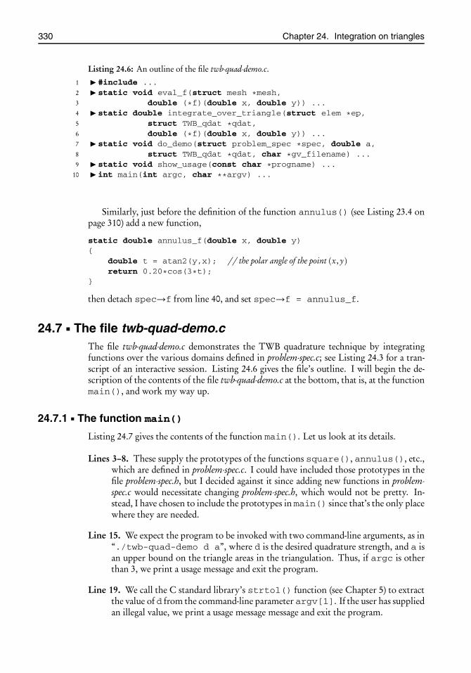
root2014/7/8page 330
�
�
�
�
�
�
�
�
330 Chapter 24. Integration on triangles
Listing 24.6: An outline of the file twb-quad-demo.c.
1 � #include ...2 � static void eval_f(struct mesh *mesh,3 double (*f)(double x, double y)) ...4 � static double integrate_over_triangle(struct elem *ep,5 struct TWB_qdat *qdat,6 double (*f)(double x, double y)) ...7 � static void do_demo(struct problem_spec *spec, double a,8 struct TWB_qdat *qdat, char *gv_filename) ...9 � static void show_usage(const char *progname) ...
10 � int main(int argc, char **argv) ...
Similarly, just before the definition of the function annulus() (see Listing 23.4 onpage 310) add a new function,
static double annulus_f(double x, double y){
double t = atan2(y,x); // the polar angle of the point (x, y)return 0.20*cos(3*t);
}
then detach spec→f from line 40, and set spec→f = annulus_f.
24.7 The file twb-quad-demo.cThe file twb-quad-demo.c demonstrates the TWB quadrature technique by integratingfunctions over the various domains defined in problem-spec.c; see Listing 24.3 for a tran-script of an interactive session. Listing 24.6 gives the file’s outline. I will begin the de-scription of the contents of the file twb-quad-demo.c at the bottom, that is, at the functionmain(), and work my way up.
24.7.1 The function main()
Listing 24.7 gives the contents of the function main(). Let us look at its details.
Lines 3–8. These supply the prototypes of the functions square(), annulus(), etc.,which are defined in problem-spec.c. I could have included those prototypes in thefile problem-spec.h, but I decided against it since adding new functions in problem-spec.c would necessitate changing problem-spec.h, which would not be pretty. In-stead, I have chosen to include the prototypes in main() since that’s the only placewhere they are needed.
Line 15. We expect the program to be invoked with two command-line arguments, as in“./twb-quad-demo d a”, where d is the desired quadrature strength, and a isan upper bound on the triangle areas in the triangulation. Thus, if argc is otherthan 3, we print a usage message and exit the program.
Line 19. We call the C standard library’s strtol() function (see Chapter 5) to extractthe value of d from the command-line parameter argv[1]. If the user has suppliedan illegal value, we print a usage message message and exit the program.

root2014/7/8page 331
�
�
�
�
�
�
�
�
24.7. The file twb-quad-demo.c 331
Listing 24.7: The function main() in the file twb-quad-demo.c.
1 int main(int argc, char **argv)2 {3 struct problem_spec *square(void);4 struct problem_spec *triangle_with_hole(void);5 struct problem_spec *annulus(int n);6 void free_annulus(struct problem_spec *spec);7 struct problem_spec *three_holes(int n);8 void free_three_holes(struct problem_spec *spec);9 struct problem_spec *spec;
10 struct TWB_qdat *qdat;11 int d; // the quadrature strength12 int n; // the number of quadrature points13 double a; // upper bound on triangle areas14 char *endptr;15 if (argc �= 3) {16 show_usage(argv[0]);17 return EXIT_FAILURE;18 }19 d = strtol(argv[1], &endptr, 10);20 if (*endptr �= ’\0’) {21 show_usage(argv[0]);22 return EXIT_FAILURE;23 }24 a = strtod(argv[2], &endptr);25 if (*endptr �= ’\0’ || a ≤ 0) {26 show_usage(argv[0]);27 return EXIT_FAILURE;28 }29 qdat = twb_qdat(&d, &n);30 printf("quadrature strength = %d, number of points = %d\n", d, n);31 putchar(’\n’);32
33 do_demo(triangle_with_hole(), a, qdat, "triangle-with-hole.gv");34 putchar(’\n’);35
36 spec = annulus(12);37 do_demo(spec, a, qdat, "annulus.gv");38 free_annulus(spec);39 putchar(’\n’);40 ...
Line 24. We call the C standard library’s strtod() function (see Chapter 5) to extractthe value of a from the command-line parameter argv[2]. If the user has suppliedan illegal value, we print a usage message message and exit the program.
Line 29. We call twb_qdat() to fetch the quadrature table of strength d. The valueof d will be adjusted, if necessary, to conform to one of the 14 possible values; seeTable 24.1 on page 322.
Line 33. We call do_demo() (more on that later) to perform an integration over the do-main returned by triangle_with_hole() as defined in the file problem-spec.c.
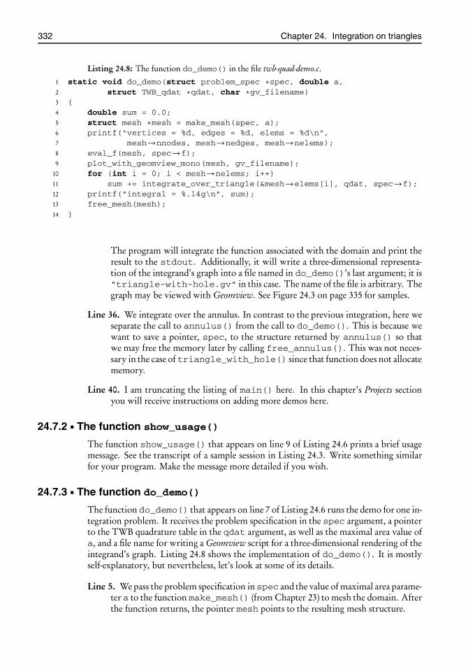
root2014/7/8page 332
�
�
�
�
�
�
�
�
332 Chapter 24. Integration on triangles
Listing 24.8: The function do_demo() in the file twb-quad-demo.c.
1 static void do_demo(struct problem_spec *spec, double a,2 struct TWB_qdat *qdat, char *gv_filename)3 {4 double sum = 0.0;5 struct mesh *mesh = make_mesh(spec, a);6 printf("vertices = %d, edges = %d, elems = %d\n",7 mesh→nnodes, mesh→nedges, mesh→nelems);8 eval_f(mesh, spec→f);9 plot_with_geomview_mono(mesh, gv_filename);
10 for (int i = 0; i < mesh→nelems; i++)11 sum += integrate_over_triangle(&mesh→elems[i], qdat, spec→f);12 printf("integral = %.14g\n", sum);13 free_mesh(mesh);14 }
The program will integrate the function associated with the domain and print theresult to the stdout. Additionally, it will write a three-dimensional representa-tion of the integrand’s graph into a file named in do_demo()’s last argument; it is"triangle-with-hole.gv" in this case. The name of the file is arbitrary. Thegraph may be viewed with Geomview. See Figure 24.3 on page 335 for samples.
Line 36. We integrate over the annulus. In contrast to the previous integration, here weseparate the call to annulus() from the call to do_demo(). This is because wewant to save a pointer, spec, to the structure returned by annulus() so thatwe may free the memory later by calling free_annulus(). This was not neces-sary in the case of triangle_with_hole() since that function does not allocatememory.
Line 40. I am truncating the listing of main() here. In this chapter’s Projects sectionyou will receive instructions on adding more demos here.
24.7.2 The function show_usage()
The function show_usage() that appears on line 9 of Listing 24.6 prints a brief usagemessage. See the transcript of a sample session in Listing 24.3. Write something similarfor your program. Make the message more detailed if you wish.
24.7.3 The function do_demo()
The function do_demo() that appears on line 7 of Listing 24.6 runs the demo for one in-tegration problem. It receives the problem specification in the spec argument, a pointerto the TWB quadrature table in the qdat argument, as well as the maximal area value ofa, and a file name for writing a Geomview script for a three-dimensional rendering of theintegrand’s graph. Listing 24.8 shows the implementation of do_demo(). It is mostlyself-explanatory, but nevertheless, let’s look at some of its details.
Line 5. We pass the problem specification in spec and the value of maximal area parame-ter a to the function make_mesh() (from Chapter 23) to mesh the domain. Afterthe function returns, the pointer mesh points to the resulting mesh structure.

root2014/7/8page 333
�
�
�
�
�
�
�
�
24.7. The file twb-quad-demo.c 333
Listing 24.9: The function integrate_over_triangle() in the file twb-quad-demo.c.
1 static double integrate_over_triangle(struct elem *ep,2 struct TWB_qdat *qdat, double (*f)(double x, double y))3 {4 double x[3], y[3];5 double sum = 0.0;6 for (int i = 0; i < 3; i++) {7 x[i] = ep→n[i]→x;8 y[i] = ep→n[i]→y;9 }
10 while (qdat→weight �= -1) {11 double lambda[3];12 lambda[0] = qdat→lambda1;13 lambda[1] = qdat→lambda2;14 lambda[2] = qdat→lambda3;15 double X = lambda[0]*x[0] + lambda[1]*x[1] + lambda[2]*x[2];16 double Y = lambda[0]*y[0] + lambda[1]*y[1] + lambda[2]*y[2];17 sum += qdat→weight * f(X,Y);18 qdat++;19 }20 return (ep→area / TWB_STANDARD_AREA) * sum;21 }
Line 8. The call to eval_f(), explained fully in subsection 24.7.5, evaluates the inte-grand, that is, spec→f, at every node of the mesh and stores the value in the nodestructure’s z member; see line 4 of Listing 23.6 on page 312. This step is not nec-essary at all for the integration. It is done only for producing a three-dimensionaldrawing of the integrand’s graph; see the next step.
Line 9. The function plot_with_geomview_mono() is defined in the file plot-with-geomview.c, which you downloaded from the book’s website; see Section 24.5. Itreads the mesh data and produces a script which may be fed to Geomview to pro-duce a three-dimensional monochrome rendering of the integrand. The value ofthe integrand at each node is obtained from node structure’s z member, as notedabove. Replace the call with plot_with_geomview_zhue() to obtain a col-ored graph.
This step is not necessary at all for the integration. If you are not interested in seeingthe integrand’s graph, you may safely remove lines 8 and 9 from do_demo().
Line 10. Here is where the real work is done. The for-loop goes over the mesh’s el-ements (that is, triangles), calls integrate_over_triangle() (more aboutthat later) to integrate over individual triangles, and accumulates the results. After-ward the accumulated value is printed and the memory associated with the mesh isfreed.
24.7.4 The function integrate_over_triangle()
The function integrate_over_triangle() that appears on line 4 of Listing 24.6 iswhere the main action takes place. It integrates a function over a triangle through a TWBquadrature. Its implementation is shown in its entirety in Listing 24.9.
root2014/7/8page 334
�
�
�
�
�
�
�
�
334 Chapter 24. Integration on triangles
The function’s first argument, ep, is a pointer to a struct elem (that is, a triangle)declared in the file mesh.h; see line 16 of Listing 23.6 on page 312. The function’s secondargument is a pointer to a TWB quadrature table, and the third argument is a function ofthe type R2 →R. The goal is to integrate that function over the triangle and return theresult. Let us examine the details.
Line 6. The expression ep→n[i] is a pointer to the node at the element’s ith vertex.Therefore the vertex’s coordinates are ep→n[i]→x and ep→n[i]→y. Theseexpressions are rather clumsy; therefore we introduce the shorthands x[i] andy[i] for these.
Line 10. The while-loop goes over the quadrature points. It stops when we reach thequadrature table’s end-marker, which is a point with weight −1 (see Example 24.2on page 324). We introduce lambda[i] as a shorthand for the barycentric coordi-nates qdat→lambda1, etc., and then calculate the Cartesian coordinates (X ,Y )of the quadrature point in accordance with (A.1) on page 375. Then we evaluatethe function f at the quadrature point, multiply the result by the correspondingweight, and accumulate the results in the variable sum. In effect, this is the C im-plementation of the summation in formula (24.1) on page 320.
Line 20. This corresponds to the multiplication by |T |/|Tstd| in formula (24.1).
24.7.5 The function eval_f()
The function eval_f() that appears on line 2 of Listing 24.6 receives pointers to a meshand a function. It evaluates the function at every node and places the result in the nodestructure’s z member. The computation is quite straightforward, so I will let you writethe code.
24.8 Project TWB Quadrature
Part 24.1. You have all the bits and pieces needed to compile and test the TWB quadra-ture program. I suggest that you begin with twb-quad-minimal.c presented in Exam-ple 24.4 to gain some assurance that things work as they should. Then proceed withthe various items below.
Part 24.2. Complete the loose ends. Based on Section 24.6’s narrative, the domain-specification functions triangle_with_hole() and annulus() and the associatedfunctions (integrands) triangle_f() andannulus_f() should be ready to go. Com-pile, link, and execute the program. Compare its output to that shown in the transcriptof the interactive session in Listing 24.3.
Part 24.3. In problem-spec.c you have a function square() that defines a domain inthe form of the unit square [0,1]× [0,1]. Add the associated function square_f() asf (x.y) = 36xy(1− x)(1− y) whose exact integral over the square is 1. Verify that yourprogram confirms that. You will need to add code at the bottom of main() in the filetwb-quad-demo.c to activate this demo.
Part 24.4. Change square_f() to f (x, y) = 403 x(1− x2)y(1− y3). (Don’t delete the
previous function; just comment it out.) This also integrates to 1 on [0,1]× [0,1]. Whatis a good quadrature strength for it?

root2014/7/8page 335
�
�
�
�
�
�
�
�
24.8. Project TWB Quadrature 335
(a) (b)
Figure 24.3: The graphs of the integrands of the problem specifications intriangle_with_hole() and three_holes(), produced byexecuting “./twb-quad-demo 4 0.01” and then viewing theresults in Geomview. The color figure on the left is made byplot_with_geomview_zhue() and then printed in greyscaleon this page, and the monochrome one on the right is made byplot_with_geomview_mono().
Part 24.5. Try a nonpolynomial for square_f(). The function f (x, y) = π2
4 sinπx sinπyintegrates to 1 over the square. What does your program say?
Part 24.6. In problem-spec.c you have a function three_holes() that defines anL-shaped domain with three holes; see Figure 23.1 on page 302. Add the associated func-tion three_holes_f() as f (x, y) = x2+y2, and extend main() to activate the demo.Compare the result with that shown in Listing 24.3. View the graphics file that the pro-gram generates. Mine is shown in Figure 24.3(b).

root2014/7/8page 337
�
�
�
�
�
�
�
�
Chapter 25
Finite elements
Prerequisites: Chapters 7, 8, 11, 12, 23, 24, and Appendix A
25.1 The Poisson equationThe simplest introduction to the finite element method (FEM) for solving partial differen-tial equations (PDEs) is through the Poisson equation89 in two dimensions:
∂ 2u
∂ x2 +∂ 2u
∂ y2 + f = 0, (25.1)
where f = f (x, y) is given, and u = u(x, y) is unknown. You can see right away that asolution u, if one exists, is not unique. For instance, if u(x, y) is a solution, then u(x, y)+ax + b y+ c + eαx sinαy + eβx cosβy with arbitrary constants a, b , c , α, and β also is asolution since those extra terms go away when you differentiate them twice and add. Theslack in determining u(x, y) is much wider than the five extra terms that I have shown.Any member of the rich class of functions known as harmonic functions is a part of thatslack.
Practical applications supplement the Poisson equation with additional data that helpto single out a unique solution out of the infinitely many candidates. Consider, for exam-ple, a prescribed domain Ω ∈R2 and a given function f :Ω→R, and pose the followingboundary value problem: Find u :Ω→R such that90
∂ 2u
∂ x2 +∂ 2u
∂ y2 + f = 0 in Ω,
u = 0 on ∂ Ω.
(25.2)
The boundary value problem (25.2) occurs in innumerable contexts in mathematicalmodels in physics and engineering. Almost every elementary book on PDEs and everybook in the “mathematical methods in physics/engineering” genre will give the deriva-tion of the boundary value problem (25.2), or variants thereof, in numerous contexts,
89The equation is named after the French mathematician Siméon Denis Poisson, pronounced pwa-son. Thethree-dimensional version of the equation is ∂ 2 u
∂ x2 +∂ 2 u∂ y2 +
∂ 2 u∂ z2 + f = 0, where u and f are functions of x , y,
and z.90The notation “∂ Ω” is a conventional way of referring to the boundary of Ω. The “∂ ” there has nothing to
do with partial derivatives.
337

root2014/7/8page 338
�
�
�
�
�
�
�
�
338 Chapter 25. Finite elements
such as heat conduction, equilibrium of membranes under applied loads, and distribu-tion of charges on electrically conducting objects. The books [38, 81, 20, 43, 79, 83] arebut a small sample of the titles in this vast area.
It turns out that if (a) the geometry ofΩ is nice, e.g., it is bounded and has a nonemptyinterior; (b) ∂ Ω has no severe kinks or weird things like fractals; and (c) the function f isnice, e.g., it does not have severe discontinuities, then the boundary value problem (25.2)has a unique solution u. The FEM may be applied to find an approximation to that uwith a desired level of accuracy. It is the goal of this chapter to learn how.
25.2 The weak formulation25.2.1 Gradient, divergence, and Laplacian
The gradient of a function u : Rn → R is the vector ∇u = ⟨ ∂ u∂ x1
, ∂ u∂ x2
, . . . , ∂ u∂ xn⟩, where
x1, x2, . . . , xn are the Cartesian coordinates. Insofar as ∇u is the list of the first orderpartial derivatives of u, it does not matter whether you think of it as a row or columnvector. However, when∇u appears in the context of matrix algebra, it is always regardedas a column vector so that an expression of the sort A∇u, where A is an n × n matrix,makes sense.
The gradient operator is the symbolic vector ∇ = ⟨ ∂∂ x1, ∂∂ x2
, . . . , ∂∂ xn⟩. One thinks of
∇u as the operator∇ acting on the function u. If v is a vector field, that is, v : Rn →Rn ,then∇ can operate on v as in a dot product:
∇ ·v =6 ∂
∂ x1,∂
∂ x2, . . . ,
∂
∂ xn
7· ⟨v1, v2, . . . , vn⟩=
∂ v1
∂ x1+∂ v2
∂ x2+ · · ·+ ∂ vn
∂ xn.
The expression∇·v occurs frequently in applications, especially in continuum mechanicsand electromagnetism. It is called the divergence of the vector field v. (The notation divv isanother way of writing∇·v.) In particular, if v is a potential vector field, that is, v =∇u,where u is a scalar function, then we get
div∇u =∇ ·∇u =∇ ·6 ∂ u∂ x1
,∂ u∂ x2
, . . . ,∂ u∂ xn
7=∂ 2u
∂ x21
+∂ 2u
∂ x22
+ · · ·+ ∂2u
∂ x2n
.
The result, which is really the divergence of the gradient of u, is called the Laplacian of u.Like the divergence, this too occurs in very many places in applications to mechanics andphysics. Although ∇ · ∇u is a perfectly good notation for the concept, you may see itwritten variously as ∇2u (engineers and physicists like that) orΔu (mathematicians likethat). Accordingly, the Poisson equation (25.1) may be written variously as
∇ ·∇u + f = 0 or div∇u + f = 0 or ∇2u + f = 0 or Δu + f = 0.
These are more compact than (25.1), and more general as well, since they are not limitedto two dimensions.
25.2.2 The Divergence Theorem
The Divergence Theorem is an indispensable tool when working with PDEs. A first coursein multivariable calculus is likely to present the Divergence Theorem only for the n = 2

root2014/7/8page 339
�
�
�
�
�
�
�
�
25.2. The weak formulation 339
and n = 3 cases. In the n = 2 case it is called Green’s Theorem and is stated as∫∫Ω
divF (x, y)da =∫∂ Ω
F ·nd s ,
where F : Ω ⊂ R2 → R2 is a vector field on the two-dimensional domain Ω and n isthe unit outward normal to the boundary, ∂ Ω (see, e.g., the section titled “Curl and Di-vergence” in Stewart [65]). In the n = 3 case it is called the Divergence Theorem and isstated as ∫∫∫
Ω
divF (x, y, z)d v =∫∫
∂ Ω
F ·nda,
where F :Ω⊂R3 →R3 is a vector field on the three-dimensional domain Ω and n is theunit outward normal to the boundary, ∂ Ω (see, e.g., the section titled “The DivergenceTheorem” in Stewart [65]).
A more advanced course in multivariable calculus is likely to present the DivergenceTheorem on Rn for any n in the form∫
Ω
divF d x =∫∂ Ω
F ·nda, (25.3)
whereF :Ω⊂Rn →Rn is a vector field on the n-dimensional domainΩ and n is the unitoutward normal to the boundary, ∂ Ω. The left-hand side represents an n-tuple integralover Ω. The right-hand side is a surface integral over Ω’s boundary.
Although the implementations of FEM are limited to two-dimensional domains inthis book, I will use the general form (25.3) of the Divergence Theorem in the discussionsince it is less cumbersome than the others.
A very useful consequence of the Divergence Theorem (25.3) is obtained by settingF = v∇u, where u and v are arbitrary (scalar) functions on Ω⊂Rn . We have
divF =∇·(v∇u) =n∑
i=1
∂
∂ xi
�v∂ u∂ xi
�=
n∑i=1
∂ v∂ xi
∂ u∂ xi+
n∑i=1
v∂ 2u
∂ x2i
=∇u ·∇v+v∇·∇u;
therefore, the Divergence Theorem implies that∫Ω
(∇u ·∇v + v∇ ·∇u)d x =∫∂ Ω
v∇u ·nda =∫∂ Ω
v∂ u∂ n
da. (25.4)
This identity, which holds between any two scalar functions u and v on any domainΩ⊂Rn ,91 is called Green’s identity.
25.2.3 The weak formulation
For convenience, I will reproduce the boundary value problem (25.2) here with the equiv-alent but more compact notation
∇ ·∇u + f = 0 on Ω,u = 0 on ∂ Ω.
(25.5)
Let V be the set of (smooth) functions defined on Ω that vanish on ∂ Ω. The solution ubelongs to that set. Pick an arbitrary function v ∈V . Plug v and the solution u of (25.5)
91I am glossing over technical issues such as differentiability and integrability of the functions and the smooth-ness of the domain.

root2014/7/8page 340
�
�
�
�
�
�
�
�
340 Chapter 25. Finite elements
into Green’s identity in (25.4). The boundary integral drops out since v is zero on theboundary, and we are left with
∫Ω(∇u ·∇v − v f )d x = 0, which we rearrange as∫
Ω
∇u ·∇v d x =∫Ω
f v d x. (25.6)
We conclude that a solution u of the boundary value problem (25.5) satisfies the iden-tity (25.6) for every possible function v in V . It can be shown that the converse is alsotrue: If (25.6) holds for a function u ∈ V and all functions v ∈ V , then u is a solutionof (25.5). In those terms, the boundary value problem (25.5) and the identity (25.6) areequivalent. The identity (25.6) is called the weak formulation of the boundary value prob-lem (25.5). In light of this, solving the boundary value problem (25.5) is equivalent to thefollowing statement:
Find u ∈V such that∫Ω
∇u ·∇v d x =∫Ω
f v d x for all v ∈V . (25.7)
I am being intentionally evasive about the precise nature of the set V . If V is goingto serve as a source of functions for u and v, then we had better impose some constraintson the types of functions that go into it. For instance, such functions need to be dif-ferentiable in some sense so that the expressions ∇u and ∇v in (25.7) have meanings.Additionally, such functions need to be integrable in some sense because otherwise theintegrals in (25.7) won’t have meanings. Furthermore, the set V should be sufficientlyrich; otherwise the weak formulation (25.7) can’t be equivalent to the boundary valueproblem (25.5). The precise characterization of V involves the Sobolev space H 1(Ω) andits subspaces. I will not elaborate on these here. See the references at the end of this chap-ter for further study. I have strived to present the FEM in this chapter in such a way that itshould remain accessible, at least in a general outline, even if you don’t grasp the technicaldetails. A lack of knowledge of the Sobolev spaces, for instance, should not hinder thecompletion of this chapter’s projects.
Remark 25.1. There is magic in (25.7). The PDE in (25.5) is of second order since uis being differentiated twice. In the slight of hand that leads to (25.7), the second orderderivatives disappear. That effect has wide-ranging repercussions in the theory of PDEs.
25.3 The Galerkin approximationOnce the vague ideas introduced in the previous section are placed on a firm mathematicalfoundation, it emerges that the set V of functions introduced in the previous section isa linear space, that is, if f and g are in V , then α f + βg is in V for all constants αandβ. Furthermore, the linear space V is infinite dimensional; there is no finite basis thatspans V . The Galerkin approximation92 amounts to replacing the infinite-dimensionalspace V with an m-dimensional subspace, say Vm ⊂V , and then reformulating (25.7) asfollows:
92It is named after the Russian engineer/mathematician Boris Galerkin, the proper romanization of whosename is Galyorkin, but in English-speaking countries it is generally spelled and pronounced “Galerkin”.
root2014/7/8page 341
�
�
�
�
�
�
�
�
25.4. An overview of the FEM 341
Find um ∈Vm such that∫Ω
∇um ·∇v d x =∫Ω
f v d x for all v ∈Vm. (25.8)
One wants Vm to approximate V well enough so that the solution um of (25.8) is nearthe solution u of (25.7) if m is large. We will look at the construction of such a Vmin the next section. For now, suppose that we have succeeded in constructing a basis�m = {vi}m
i=1 for Vm . Then the condition “for all v ∈ Vm” in (25.8) is equivalent to“for v = vi , i = 1,2, . . . , m”. Furthermore, any um ∈ Vm may be expressed as a linearcombination of Vm’s basis functions:
um =m∑
j=1
c j v j . (25.9)
Consequently, the equation in (25.8) takes the form∫Ω
∇* m∑
j=1
c j v j
+·∇vi d x =
∫Ω
f vi d x, i = 1,2, . . . , m,
which, upon a slight rearrangement of terms, leads us to the following equivalent formu-lation of Galerkin’s approximation:
Find c j , j = 1,2, . . . , m, such that
m∑j=1
�∫Ω
∇vi ·∇vj d x�
c j =∫Ω
f vi d x, i = 1,2, . . . , m. (25.10)
At this point we introduce an m×m matrix K and an m-vector F through
Ki j =∫Ω
∇vi ·∇vj d x, Fi =∫Ω
f vi d x, (25.11)
and an m-vector c with components c = ⟨c1, c2, . . . , cm⟩, whereupon Galerkin’s approxi-mation (25.10) takes the form of a linear system of m equations in m unknowns:
Kc = F . (25.12)
Thus, finding the approximate solution um of the boundary value problem (25.5) hasbeen reduced to computing the integrals in (25.11), solving the linear system (25.12) for c ,and then evaluating the sum (25.9).
The m×m matrix K is called the system stiffness matrix and the vector F is called thesystem force vector, terminology that dates back to the early years of the FEM and its usein solving elasticity problems.
25.4 An overview of the FEMTo begin implementing the previous section’s Galerkin approximation idea, we need toconstruct a basis �m = {vi }m
i=1 for the subspace Vm and compute the stiffness matrix Kand the force vector F in (25.11). We will see how these are done in the following foursubsections.

root2014/7/8page 342
�
�
�
�
�
�
�
�
342 Chapter 25. Finite elements
Figure 25.1: A triangulated square and a few basis functions, shown in perspective (left)and viewed from above (right). Note the overlap of the supports of theadjacent basis functions.
25.4.1 Meshing
The FEM’s first step in the construction of the finite-dimensional subspace Vm and itsbasis�m is to mesh the domain Ω. In this book we will consider triangular meshes only,although quadrilateral and hexagonal meshes are also in common use. Figure 25.1 showsa sample triangulated domainΩwhich happens to be a square in this instance, but the factthat it is a square has no bearing on what follows. The figure also shows a few pyramidswhich are constructed as follows. Pick any vertex, say vertex number i , of the mesh. Iden-tify all the triangles that have that vertex in common. Construct a pyramid of height 1,whose apex is situated directly above the selected vertex and whose base consists of theunion of the triangles that you identified. Consider the pyramid as the graph of a functionof two variables. Extend that function by zero to the rest of the domainΩ. Call the result-ing function vi . Repeat this for every vertex of the mesh other than those vertices thatfall on the domain’s boundary. This produces a collection of functions �m = {vi }m
i=1,where m is the number of the mesh’s internal vertices. Each function vi ∈�m is definedover the entire Ω, and has a graph in the form of a pyramid locally, and extended by zeroglobally. It should be clear that �m is a linearly independent set—you cannot constructone vi ∈ �m as a linear combination of the others since vi is 1 at the vertex i while allothers are zero there.
Define the linear space Vm as the span of�m . Since�m is a basis for Vm and�m hasm elements, we have dimVm = m. Refining the mesh increases the number of internalvertices and hence the dimension of Vm .
Every function in Vm vanishes on the boundary since we skipped the boundary ver-tices when constructing the functions vi . It takes some quite technical work to show thatVm is a good approximation to V , and as m goes to infinity, the solution um of (25.8)approaches the solution u of (25.7). See any of [12, 11, 10, 23, 5] for the details.
25.4.2 Assembling the system
Now that we have constructed the pyramid-shaped basis functions vi , we should be readyto compute the system stiffness matrix K and the system force vector F through the in-tegration formulas (25.11). At first sight, computing Ki j seems to be straightforward: forevery pair of vertices i and j , we look at the pyramids centered at i and j , multiply theirgradients, and integrate. The integration takes place on the overlap region of bases of thepyramid pair since outside the overlap region at least one of the functions vi and vj is
root2014/7/8page 343
�
�
�
�
�
�
�
�
25.4. An overview of the FEM 343
zero. This gives an interesting structure to the system stiffness matrix: if the vertices iand j are not adjacent, then their pyramids do not overlap, and therefore Ki j is zero. In afine mesh it’s more likely than not that a randomly picked pair of vertices is not adjacent,and therefore most of the K matrix consists of zeros; that is, K is a sparse matrix.
The sketch above of the procedure for computing the system stiffness matrix K isvertex-oriented; in essence, it computes the entries Ki j through a doubly nested for-loopof the indices i and j which walk over the mesh’s vertices. In principle one may imple-ment such a computation, although I have never seen it done. The major impediment isthe mess in determining the overlap region of the bases of a pair of pyramids. It’s just notworth the trouble, especially since a much slicker alternative is available.
The alternative shifts the focus from vertices to triangles—instead of the doubly nestedfor-loop that walks over the vertices, we implement a single for-loop that walks overthe mesh’s triangles. Here is how it works.
We have already noted that the entry Ki j of the system stiffness matrix is the sumof the integrals over the cluster of triangles that forms the overlap region between thepyramids centered at the vertices i and j . Instead of focusing on such clusters, we com-pute integrals on every single triangle in the mesh, regardless of any considerations of towhich cluster the triangle may belong. Only retroactively do we figure out where in theK matrix the result should be inserted. Generally, each Ki j entry receives contributionsfrom multiple triangles since all triangles in an triangle cluster contribute to it. Thus, ineffect, the entries of K are assembled piecemeal, through cumulative contributions fromintegrals over individual triangles, as we walk over the mesh’s triangles. The process ofaccumulating the integrals into K is called assembling the system stiffness matrix.
To be more specific, let us say the mesh has N vertices which are numbered from 0to N − 1. The vertices of any of the mesh’s triangles may be identified in two differentways. One is through the triangle’s own internal vertex numbers, as in vertex 0, vertex 1,vertex 2, enumerated in counterclockwise order. We call these the triangle’s local vertexnumbers. The other is through the vertex numbers that the triangle inherits from themesh, as in vertex n1, vertex n2, vertex n3, where 0 ≤ n1, n2, n3 < N . We call these thetriangle’s global vertex numbers. In assembling the system stiffness matrix we will need todetermine a vertex’s global index in terms of its local index. The mesh data structure ofChapter 23 is designed specifically to facilitate that determination.
25.4.3 The element stiffness matrix
Within each triangle T , the slanted faces of the pyramidal basis functions of subsection25.4.1 appear as flat planes that rise from height 0 at one edge to height 1 at the vertexopposite that edge; see Figure A.4 on page 378 for an illustration. There are three suchfunctions on each triangle, let’s call themφ1,φ2, andφ3, whereφi is 1 at vertex i and 0 atthe other two vertices. These are called the element’s93nodal shape functions. The naturalway to express a nodal shape function is through the element’s barycentric coordinates.Following the notation of Appendix A, we have φi (λ1,λ2,λ3) = λi for i = 1,2,3.
To compute an element’s contributions to the system stiffness matrix K and the forcevector F , we introduce the 3× 3 element stiffness matrix k and the element force vector bof length 3 through
ki j =∫
T∇φi ·∇φ j d x, bi =
∫T
f φi d x, (25.13)
93Here I have switched from talking about a triangle to talking about an element. In the FEM, an element is atriangle equipped with shape functions.
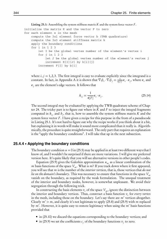
root2014/7/8page 344
�
�
�
�
�
�
�
�
344 Chapter 25. Finite elements
Listing 25.1: Assembling the system stiffness matrix K and the system force vector F .
initialize the matrix K and the vector F to zerofor each element e in the mesh
compute the 3x1 element force vector b (TWB quadrature)compute the 3x3 element stiffness matrix kapply the boundary conditionsfor i in 1 2 3
let I be the global vertex number of the element’s vertex ifor j in 1 2 3
let J be the global vertex number of the element’s vertex jincrement K[I][J] by k[i][j]
increment F[I] by b[i]
where i , j = 1,2,3. The first integral is easy to evaluate explicitly since the integrand is aconstant. In fact, in Appendix A it is shown that ∇φi · ∇φ j =
14|T |2 ei · e j , where ei and
e j are the element’s edge vectors. It follows that
ki j =1
4|T |ei ·e j . (25.14)
The second integral may be evaluated by applying the TWB quadrature scheme of Chap-ter 24. The tricky part is to figure out where in K and F to inject the integral fragmentscomputed in ki j and bi , that is, how to assemble the system stiffness matrix K and thesystem force vector F . I have given a recipe for this purpose in the from of a pseudocodein Listing 25.1. It’s not hard to figure out why the recipe works if you think about it a bit,but explaining it in words will make it sound more complicated than it really is. Algorith-mically, the procedure is quite straightforward. The only part that requires an explanationis the “apply the boundary conditions”. I will take that up in the next subsection.
25.4.4 Applying the boundary conditions
The boundary condition u = 0 in (25.5) may be applied in at least two different ways that Iknow of, and I wouldn’t be surprised if there are more variations. I will give my preferredversion here. It’s quite likely that you will see alternative versions in other people’s codes.
Equation (25.9) gives the Galerkin approximation um as a linear combination of them basis functions of the space Vm . What is m? If you track down where it first appeared,you will see that m is the number of the interior vertices, that is, those vertices that do notlie on the domain’s boundary. This was necessary to ensure that functions in the space Vmvanish on the boundary, as required by the weak formulation. The unequal treatmentof the interior and boundary nodes, however, is somewhat unpleasant. We avoid theirsegregation through the following trick.
In constructing the basis elements vi of the space Vm , ignore the distinction betweenthe interior and boundary vertices. Thus, construct a basis function vi for every vertexin the mesh, including those on the boundary. Let’s say there are m′ vertices altogether.Clearly m′ > m, and clearly it’s not legitimate to apply (25.8) and (25.9) with m replacedby m′. However, it is quite easy to restore legitimacy when using the m′ basis functionsprovided that
• in (25.10) we discard the equations corresponding to the boundary vertices; and• in (25.9) we set the coefficients c j of the boundary functions vj to zero.

root2014/7/8page 345
�
�
�
�
�
�
�
�
25.5. Error analysis 345
At the element level, the two operations above amount to the following: If the element’svertex i falls on the domain’s boundary, then
• replace row i of the element stiffness matrix k by zeros;• replace column i of the element stiffness matrix k by zeros;• set kii = 1; and• set bi = 0.
This is what “apply the boundary conditions” means in Listing 25.1. You will find anextended explanation in the next chapter.
Remark 25.2. As a consequence of expanding the count of the basis functions from mto m′, the system stiffness matrix K is no longer m × m. It is m′ × m′. For the samereason, the system force vector F is of length m′.
25.5 Error analysisIt is reasonable to expect that a finer triangulation improves the quality of the solutionobtained by the FEM. The central problem in the mathematical analysis of the FEM isto obtain a precise relationship between the fineness of the triangulation and the error inthe FEM approximation. To make meaningful statements in that regard, the concepts of“fineness” and “error” need to be clarified.
In our program the mesh is produced through the Triangle library, which controlsthe mesh’s fineness through the maximal area parameter a that sets an upper bound onthe areas of the triangles. The default triangulation produced by Triangle is quasi-uniformin that all triangles have more or less equal areas. Furthermore, the triangles are as closeto equilaterals as possible. These two properties taken together make it meaningful totalk about the “linear size” h of the triangles. Think of h as the length of a typical trian-gle’s edge. A smaller a produces a smaller h. Since area is proportional to the square ofthe linear dimension, then a is roughly proportional to h2, or equivalently, h is roughlyproportional to
�a.
Let uh be the solution produced by the FEM on a grid of linear size h, and let uex bethe exact solution of the boundary value problem. The error uex− uh may be measuredin several different ways. Some of the most common ways are the following:
the energy norm: ‖uex− uh‖E =�∫Ω
���∇uex(x)−∇uh (x)���2 d x
�1/2
, (25.15a)
the L2 norm: ‖uex− uh‖L2 =�∫Ω
���uex(x)− uh (x)���2 d x
�1/2
, (25.15b)
the L∞ norm: ‖uex− uh‖L∞ = supx∈Ω
���uex(x)− uh (x)���. (25.15c)
All three are meaningful in the context of n-dimensional domains. The symbol x standsfor a generic point in Rn . In two dimensions we write x explicitly as (x, y).
It can be shown (see, e.g., [23, pages 111 and 117], [10, page 93], and [57]) that thereare constants c1, c2, and c3 associated with a two-dimensional polygonal domain Ω suchthat when h is small, one has
‖uex− uh‖E ≤ c1h‖uex‖H 2 , (25.16a)
‖uex− uh‖L2 ≤ c2h2‖uex‖H 2 , (25.16b)
‖uex− uh‖L∞ ≤ c3h2| ln h|3/2‖D2uex‖L∞ , (25.16c)

root2014/7/8page 346
�
�
�
�
�
�
�
�
346 Chapter 25. Finite elements
Table 25.1: The errors in various norms, as computed by this chapter’s FEM solver, cor-responding to the square domain problem described on page 350 for whichthe exact solution is known. Figure 25.2 is a graphical representation of thistable. The column with the header “nelems” lists the number of elementsin each case.
a nelems ‖uex− uh‖L∞ ‖uex− uh‖L2 ‖uex− uh‖E
0.08 16 0.199408 0.114036 1.05550.04 34 0.187421 0.0873139 0.9419210.02 79 0.0647486 0.0275582 0.5219540.01 159 0.0526887 0.0154082 0.3886790.005 318 0.0207487 0.00702712 0.2630950.0025 642 0.0140025 0.00375021 0.1912470.00125 1277 0.00524254 0.00181353 0.1332320.00064 2427 0.00359181 0.000937034 0.09571340.00032 4967 0.00155731 0.000462236 0.06710780.00016 9946 0.000911879 0.000235085 0.0478856
where ‖uex‖H 2 is a Sobolev norm94 of the solution uex, and D2uex means the list of thesecond order partial derivatives of uex. In two dimensions, h is proportional to
�a, as
noted above; therefore the error in the L2 norm is of order a and the error in the energynorm is of order
�a. In particular, if you reduce a by a factor of 1/4, then the error in
the L2 norm will be reduced by a factor of 1/4, while the error in the energy norm willbe reduced by a factor of 1/2.
Table 25.1 shows the errors in various norms, as computed by this chapter’s FEMsolver, corresponding to the square domain problem described on page 350 for which theexact solution is known. I used d = 10 for the TWB quadrature strength in all cases. Fig-ure 25.2 is a visual representation of that table, done in log-log plots. The dashed linescorrespond to the functions c1
�a and c2a for some (irrelevant) choices of constants c1
and c2. For small values of a, the graph corresponding to ‖uex − uh‖E parallels c1�
a,and the graph corresponding to ‖uex − uh‖L2 parallels c2a, in agreement with the esti-mates (25.16).
Computing the norm ‖uex−uh‖L2 is a matter of an integration over the PDE’s domain.Computing the ‖uex−uh‖E appears to be more complex at first sight since it involves∇uex ,which is not supplied. It turns out, however, that ‖uex− uh‖E may be computed withouta reference to∇uex, due to the following trick. We have
‖uex− uh‖2E =
∫Ω
|∇(uex− uh)|2 d x
=∫Ω
|∇uex|2 d x − 2∫Ω
∇uex ·∇uh d x +∫Ω
|∇uh |2 d x.
The three integrals on the right-hand side may be simplified as follows. The exact solutionuex satisfies the identity (25.7) for all choices of v in V . This has two consequences. First,by picking v = uex we get
∫Ω|∇uex|2 d x =
∫Ω
f uex d x. Second, by picking v = uh we get
94You don’t need to know about the Sobolev norms to appreciate the significance of these error estimates.The key part is the way h enters on their right-hand sides. Thus, the first estimate says that the error, measuredin the energy norm, will decrease at least linearly in h as h goes to zero.

root2014/7/8page 347
�
�
�
�
�
�
�
�
25.6. The program 347
10−4 10−3 10−2 10−110−4
10−3
10−2
10−1
100
a (maximal triangle area)
Erro
rno
rm‖uex− uh‖E‖uex− uh‖L2
‖uex− uh‖L∞c1�
ac2a
c3a| lna|3/2
Figure 25.2: The errors in various norms, as computed by this chapter’s FEM solver,corresponding to the square domain problem described on page 350 forwhich the exact solution is known. The dashed lines correspond to thefunctions c1
�a, c2a, and a| lna|3/2 for some (irrelevant) choices of constants
c1, c2, and c3. For small values of a, the graph corresponding to ‖uex−uh‖Eparallels c1
�a, and the graph corresponding to ‖uex−uh‖L2 parallels c2a, in
agreement with the estimates (25.16). Table 25.1 is a tabular representationof these graphs.
∫Ω∇uex · ∇uh d x =
∫Ω
f uh d x. Moreover, since uh satisfies the identity (25.8) for all v,we pick v = uh and get
∫Ω|∇uh |2 d x =
∫Ω
f uh d x. In view of these, the expression forthe energy norm simplifies to
‖uex− uh‖2E =
∫Ω
(uex− uh ) f d x. (25.17)
As you see, no gradients appear in the result; therefore computing the error’s energy normis a matter of straightforward integration.
25.6 The programThe goal of this chapter’s project is to implement the FEM algorithm described in thepreceding sections in order to solve the boundary value problem (25.5), or more pre-cisely, its Galerkin approximation, (25.8). Much of the algorithm’s infrastructure hasbeen developed in the previous chapters. Specifically, we will need the files xmalloc.[ch]from Chapter 7 to allocate memory, the file array.h from Chapter 8 to construct vec-tors and matrices, the files mesh.[ch] from Chapter 23 to triangulate the domain, and thefiles twb-quad.[ch] and plot-with-geomview.[ch] from Chapter 24 to integrate over trian-gles and plot solutions. Additionally, we will need the files problem-spec.[ch] to describethe problem’s geometry and data. The file problem-spec.h remains unchanged from thatin Project Triangulate of Chapter 23; therefore a symbolic link to that file will do. The
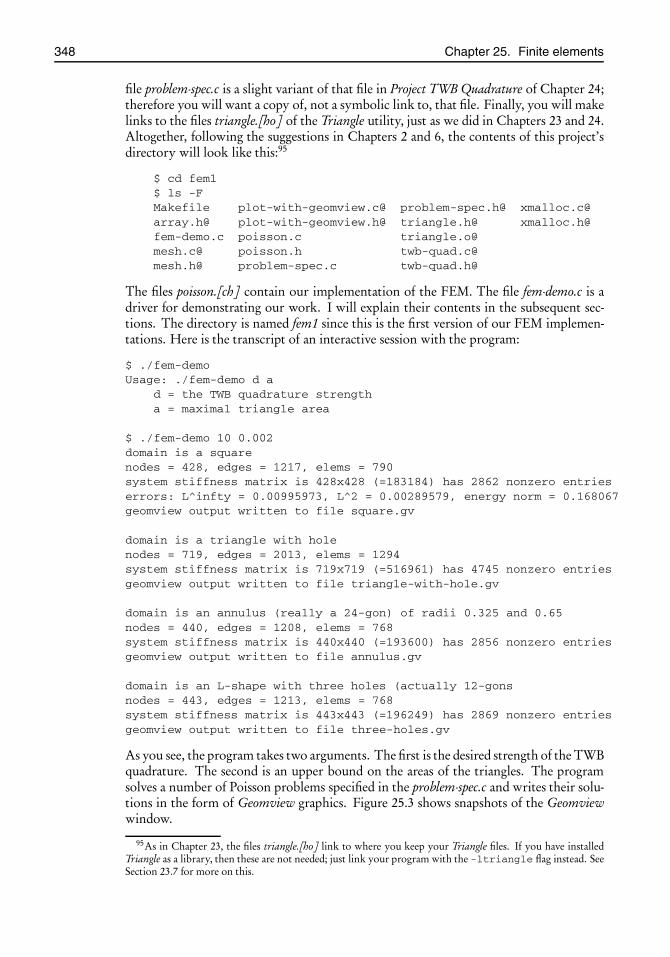
root2014/7/8page 348
�
�
�
�
�
�
�
�
348 Chapter 25. Finite elements
file problem-spec.c is a slight variant of that file in Project TWB Quadrature of Chapter 24;therefore you will want a copy of, not a symbolic link to, that file. Finally, you will makelinks to the files triangle.[ho] of the Triangle utility, just as we did in Chapters 23 and 24.Altogether, following the suggestions in Chapters 2 and 6, the contents of this project’sdirectory will look like this:95
$ cd fem1$ ls -FMakefile plot-with-geomview.c@ problem-spec.h@ [email protected]@ plot-with-geomview.h@ triangle.h@ [email protected] poisson.c [email protected]@ poisson.h [email protected]@ problem-spec.c twb-quad.h@
The files poisson.[ch] contain our implementation of the FEM. The file fem-demo.c is adriver for demonstrating our work. I will explain their contents in the subsequent sec-tions. The directory is named fem1 since this is the first version of our FEM implemen-tations. Here is the transcript of an interactive session with the program:
$ ./fem-demoUsage: ./fem-demo d a
d = the TWB quadrature strengtha = maximal triangle area
$ ./fem-demo 10 0.002domain is a squarenodes = 428, edges = 1217, elems = 790system stiffness matrix is 428x428 (=183184) has 2862 nonzero entrieserrors: L^infty = 0.00995973, L^2 = 0.00289579, energy norm = 0.168067geomview output written to file square.gv
domain is a triangle with holenodes = 719, edges = 2013, elems = 1294system stiffness matrix is 719x719 (=516961) has 4745 nonzero entriesgeomview output written to file triangle-with-hole.gv
domain is an annulus (really a 24-gon) of radii 0.325 and 0.65nodes = 440, edges = 1208, elems = 768system stiffness matrix is 440x440 (=193600) has 2856 nonzero entriesgeomview output written to file annulus.gv
domain is an L-shape with three holes (actually 12-gonsnodes = 443, edges = 1213, elems = 768system stiffness matrix is 443x443 (=196249) has 2869 nonzero entriesgeomview output written to file three-holes.gv
As you see, the program takes two arguments. The first is the desired strength of the TWBquadrature. The second is an upper bound on the areas of the triangles. The programsolves a number of Poisson problems specified in the problem-spec.c and writes their solu-tions in the form of Geomview graphics. Figure 25.3 shows snapshots of the Geomviewwindow.
95As in Chapter 23, the files triangle.[ho] link to where you keep your Triangle files. If you have installedTriangle as a library, then these are not needed; just link your program with the -ltriangle flag instead. SeeSection 23.7 for more on this.
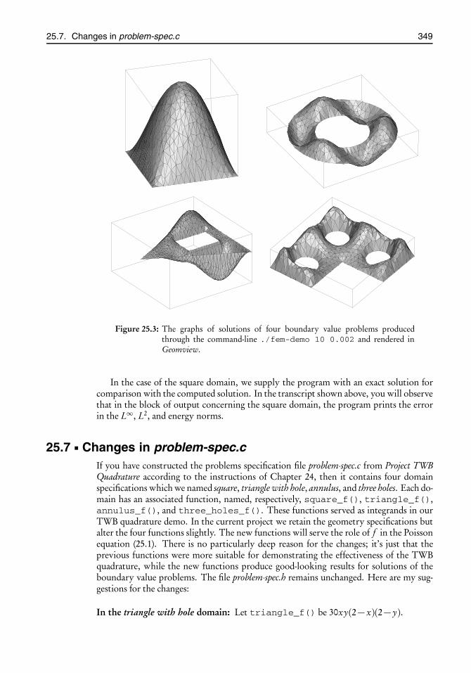
root2014/7/8page 349
�
�
�
�
�
�
�
�
25.7. Changes in problem-spec.c 349
Figure 25.3: The graphs of solutions of four boundary value problems producedthrough the command-line ./fem-demo 10 0.002 and rendered inGeomview.
In the case of the square domain, we supply the program with an exact solution forcomparison with the computed solution. In the transcript shown above, you will observethat in the block of output concerning the square domain, the program prints the errorin the L∞, L2, and energy norms.
25.7 Changes in problem-spec.cIf you have constructed the problems specification file problem-spec.c from Project TWBQuadrature according to the instructions of Chapter 24, then it contains four domainspecifications which we named square, triangle with hole, annulus, and three holes. Each do-main has an associated function, named, respectively, square_f(), triangle_f(),annulus_f(), and three_holes_f(). These functions served as integrands in ourTWB quadrature demo. In the current project we retain the geometry specifications butalter the four functions slightly. The new functions will serve the role of f in the Poissonequation (25.1). There is no particularly deep reason for the changes; it’s just that theprevious functions were more suitable for demonstrating the effectiveness of the TWBquadrature, while the new functions produce good-looking results for solutions of theboundary value problems. The file problem-spec.h remains unchanged. Here are my sug-gestions for the changes:
In the triangle with hole domain: Let triangle_f() be 30xy(2− x)(2− y).

root2014/7/8page 350
�
�
�
�
�
�
�
�
350 Chapter 25. Finite elements
Listing 25.2: The file poisson.h is the interface to our Poisson solver module.
1 #ifndef H_POISSON_H2 #define H_POISSON_H3 #include "problem-spec.h"4 #include "mesh.h"5 struct errors {6 double Linfty;7 double L2norm;8 double energy;9 };
10 void poisson_solve(struct problem_spec *spec,11 struct mesh *mesh, int d);12 struct errors eval_errors(struct problem_spec *spec,13 struct mesh *mesh, int d);14 #endif /∗ H_POISSON_H */
In the annulus domain: Let annulus_f() be what we had in Chapter 24, but changethe factor 0.20 to 20.
In the three holes domain: Let three_holes_f() be 100(x2+ y2).
In the square domain: We do things slightly differently here. Consider the functionuex = 16xy(1−x)(1−y) on the square 0≤ x, y ≤ 1. Note that uex = 0 on the bound-ary. Plugging uex for u into the PDE in (25.2), we get f = 32
�x(1− x) + y(1− y)
.
Therefore uex is the exact solution of the boundary value problem correspondingto that f . This is common method of “reverse-engineering” a PDE: we plug in afunction for u that satisfies the boundary conditions and find f . This provides anexcellent way to test the accuracy of our FEM solver.
Thus, in the file problem-spec.c define the functions square_u_exact() andsquare_f() to correspond to the functions uex and f given above. Then, in thefunction square() in that file change the u_exact member of the spec struc-ture from the previous NULL to square_u_exact.
In what follows—on line 9 in Listing 25.8, to be precise— we will set up our programso that when u_exact is non-NULL, it computes and prints the error uex − u invarious norms, where u is the solution obtained by the FEM.
25.8 The file poisson.hThe file poisson.h is the interface to our Poisson solver module. It is shown in its entiretyin Listing 25.2. It declares the prototype of the function poisson_solve(), whichtakes a problem specification, a mesh, and a number d, which is the desired strength ofthe TWB quadrature over the mesh’s triangles. It applies the FEM algorithm describedearlier in this chapter and ultimately evaluates the values of the coefficients c j of the lin-ear combination in (25.9). Since there is one c j associated with each vertex of the mesh,the program stores the value of the c j in the z member of the node structure of the nodenumber j . These may be passed to the function plot_with_geomview_mono() orplot_with_geomview_zhue() to visualize the solution in Geomview. The sam-ples in Figure 25.3 were produced that way. The headers problem-spec.h and mesh.h are

root2014/7/8page 351
�
�
�
�
�
�
�
�
25.9. The file poisson.c 351
Listing 25.3: An outline of the file poisson.c.
1 � #include ...2 � static void error_and_exit(int status, const char *file, int line) ...3 � static void enforce_zero_dirichlet_bc(struct elem *ep,4 double k[3][4]) ...5 � static void compute_element_stiffness(struct elem *ep,6 struct TWB_qdat *qdat,7 double (*f)(double x, double y), double k[3][4]) ...8 � void poisson_solve(struct problem_spec *spec,9 struct mesh *mesh, int d) ...
10 � static struct errors element_errors(struct problem_spec *spec,11 struct TWB_qdat *qdat, struct elem *ep) ...12 � struct errors eval_errors(struct problem_spec *spec,13 struct mesh *mesh, int d) ...
#included in poisson.h since the declaration of the function poisson_solve() refersto struct problem_spec and struct mesh.
Additionally, poisson.h declares a struct errors structure which is meant to holdthe L∞, L2, and energy norms of the error uex − u, as described in Section 25.5. Thefunction eval_errors() declared on line 12 of Listing 25.2 is called only when theuser supplies an exact solution for the purpose of comparison. It computes the variouserror norms and returns them in an instance of struct errors.
25.9 The file poisson.cThe file poisson.c contains the implementations of the functions poisson_solve() andeval_errors() noted in the previous section and several auxiliary functions definedfor internal use. Listing 25.3 gives an outline. I will describe its individual components inthe following subsections. The function error_and_exit(), however, is identical tothat in Project UMFPACK (see Section 12.5 on page 89); therefore I will not go over thatmaterial again. Just copy the code from umfpack-demo2.c to poisson.c.
25.9.1 The function enforce_zero_dirichlet_bc()
The function enforce_zero_dirichlet_bc() that appears on line 3 of Listing 25.3applies the algorithm described in subsection 25.4.4 which zeros the solution on the do-main’s boundary. Although the algorithm is quite straightforward, I want to introduce aperhaps not-so-obvious idea here which will help with streamlining the code.
In subsection 25.4.2 we learned that the system stiffness matrix K is assembled fromthe 3× 3 element stiffness matrices k of the mesh’s individual elements. Similarly, thesystem force vector F is assembled from the element force vectors b , which are vectorsof length 3 each. Instead of keeping track of a 3× 3 matrix k and a 3-vector b as separateobjects, it is more convenient to paste the two together into a 3× 4 matrix whose fourthcolumn is the vector b . I may still refer to the augmented matrix as the “element stiff-ness matrix” or “the matrix k”, but I hope that it will be clear from the context what Imean.

root2014/7/8page 352
�
�
�
�
�
�
�
�
352 Chapter 25. Finite elements
Following subsection 25.4.4’s instructions, if an element’s ith vertex (i = 0,1,2) fallson the domain’s boundary, we zero row i and column i of k and then set its (i , i) entryto 1. The following example shows the i = 1 case:
k00 k01 k02 k03
k10 k11 k12 k13
k20 k21 k22 k23
k00 k02 k03
k20 k22 k23
0 1 0 0
0
0
=⇒
You should be able to write the function enforce_zero_dirichlet_bc() now.As you see in its prototype on line 3 in Listing 25.3, it receives a pointer ep to an elementstructure and the address of a 3× 4 array k. You will set up a for-loop to go over theelement’s vertices, as in for (i=0, i<3, i++). At vertex i you may access the nodestructure ep→n[i] and then examine the boundary condition there ep→n[i]→bc.If it equals FEM_BC_DIRICHLET, then the node is on the boundary, and therefore youwill operate on k, as shown in the diagram above.
25.9.2 The function compute_element_stiffness()
The function compute_element_stiffness() that appears on line 5 of Listing 25.3applies the instructions of subsection 25.4.2 to compute an element’s stiffness matrix kand force vector b , which, as noted in the previous subsection, are merged into a single3× 4 matrix, also denoted by k.
The 3× 3 part of the matrix k is computed according to the explicit formula (25.14).Its fourth column, which is the element’s force vector b , is computed by applying a TWBquadrature to the expression for b in formula (25.13) on page 343. The function receivesfour data items through its arguments. These are a pointer ep to the element structure,a pointer qdat to the TWB quadrature data, a pointer f to the function f of the Poissonequation (25.2), and a pointer k to a 3× 4 array where it will store the computed data.
For the most part, the function compute_element_stiffness() duplicates thefunction integrate_over_triangle() from Chapter 24; see Listing 24.9 on page333. Therefore, copy the body of that function here, and modify it as follows. Linenumbers refer to those in Listing 24.9.
Lines 1 through 9 remain the same. Following this, insert code to calculate the 3× 3part of the matrix k through applying the formula (25.14).
In the old code, lines 10 to the end compute the integral∫
T f d x over the element T .These need slight adjustments since here we intend to compute not one but three integrals,∫
T f φi d x, i = 0,1,2. The results are to be stored in k[i][3]. Sinceφi (λ1,λ2,λ3) = λi ,then it suffices to replace line 17 with
for (i = 0; i < 3; i++)k[i][3] += qdat→weight * f(X,Y) * lambda[i];
In this connection two precautions are in order. First, since we are accumulating materialin k[i][3], we had better initialize it to zero. This should go somewhere before line 10.Second, line 20 multiplies the accumulated sum by the factor |T |/|Tstd| and returns theresult. In the modified code, each of the three k[i][3] needs to be multiplied by thatfactor. Furthermore, the return type of the new function is void, so there is nothing toreturn—the caller will read the computed data by examining the contents of the matrix k.

root2014/7/8page 353
�
�
�
�
�
�
�
�
25.9. The file poisson.c 353
25.9.3 The function poisson_solve()
The function poisson_solve() that appears on line 8 of Listing 25.3 is one of thetwo externally visible functions in the file poisson.c. (The other is eval_errors().)I have shown it in its entirety in Listings 25.4 and 25.5. The function is a somewhatlong (perhaps too long) because it performs several loosely related tasks which ultimatelyproduce the FEM approximation of the solution of the boundary value problem (25.5).It may be possible to split the function into simpler components, but I don’t see a neatway for doing that. You may. See what you can do.
The function is invoked with three arguments. These are a pointer spec to a prob-lem specification structure, a pointer mesh to a precomputed mesh structure, and a num-ber d which is the desired TWB quadrature strength for integrating over triangles. Itassembles the system stiffness matrix K and the system force vector F , calls UMFPACKto solve the linear system of equations (25.12), and then places the coefficient c j in the zmember of the node structure of the node number j for each j .
A typical system stiffness matrix K is huge and very sparse. We have no intentionof wasting memory in storing K in its entirety. Rather, we store only its nonzero en-tries in the compressed column storage (CCS) form as seen in Chapters 11 and 12. Moreprecisely, we store K ’s nonzero entries in UMFPACK’s triplet form as explained in Sec-tion 12.6 (page 90) and then convert from the triplet form to the CCS form by applyingUMFPACK’s umfpack_di_triplet_to_col() function. Let’s see how this is doneby examining Listing 25.4:
Line 10. We are going to need the TWB quadrature data for integration over the triangles,so we might as well retrieve it right now. Following the remark in Example 24.3 onpage 324, we set the second argument of twb_qdat() to NULL since we have noneed for the number of quadrature points in the rest of the code. If you do want toknow the number of quadrature points, then follow Example 24.2 on page 324.
Lines 12–14. The major task of the function poisson_solve() is to implement theidea shown in the pseudocode in Listing 25.1 on page 344. There, we go over themesh’s triangles, and in each triangle we compute the element stiffness matrix kand then in effect “inject” k into the global stiffness matrix K, that is to say, in-crement the values of K[I][J] by k[i][j] for i,j=0,1,2. We have no in-tention, however, of allocating memory to store the massively sparse matrix K. Wemerely store the incrementation data, that is, the indices I and J, and the incrementamount k[i][j] into UMFPACK’s triplet vectorsTi, Tj, andTx; see Section 12.6,page 90.
That is all to come later. What we need to do right now is to determine suitablelengths for the triplet vectors. They should be long enough to hold all the incre-mentation data that is handed to them. How may increments are there? The ele-ment stiffness matrix is 3×3. The mesh has mesh→nelems elements. Therefore,there will be a total of 3*3*mesh→nelems increments. Ergo, the triplet vectorsshould be that long. That’s what we see on lines 12–14.
Lines 16–18. UMFPACK’s triplet vectors are there for the programmer’s convenience.What we really need are the corresponding CCS vectors Ap, Ai, and Ax. As wesaw in Section 12.6, UMFPACK’s umfpack_di_triplet_to_col() convertsthe triplet format to the CCS format. In lines 16–18 we allocate memory for theCCS vectors.
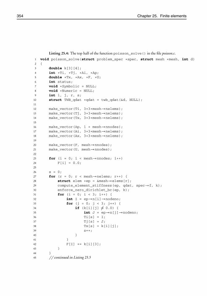
root2014/7/8page 354
�
�
�
�
�
�
�
�
354 Chapter 25. Finite elements
Listing 25.4: The top half of the function poisson_solve() in the file poisson.c.
1 void poisson_solve(struct problem_spec *spec, struct mesh *mesh, int d)2 {3 double k[3][4];4 int *Ti, *Tj, *Ai, *Ap;5 double *Tx, *Ax, *F, *U;6 int status;7 void *Symbolic = NULL;8 void *Numeric = NULL;9 int i, j, r, s;
10 struct TWB_qdat *qdat = twb_qdat(&d, NULL);11
12 make_vector(Ti, 3*3*mesh→nelems);13 make_vector(Tj, 3*3*mesh→nelems);14 make_vector(Tx, 3*3*mesh→nelems);15
16 make_vector(Ap, 1 + mesh→nnodes);17 make_vector(Ai, 3*3*mesh→nelems);18 make_vector(Ax, 3*3*mesh→nelems);19
20 make_vector(F, mesh→nnodes);21 make_vector(U, mesh→nnodes);22
23 for (i = 0; i < mesh→nnodes; i++)24 F[i] = 0.0;25
26 s = 0;27 for (r = 0; r < mesh→nelems; r++) {28 struct elem *ep = &mesh→elems[r];29 compute_element_stiffness(ep, qdat, spec→f, k);30 enforce_zero_dirichlet_bc(ep, k);31 for (i = 0; i < 3; i++) {32 int I = ep→n[i]→nodeno;33 for (j = 0; j < 3; j++) {34 if (k[i][j] �= 0.0) {35 int J = ep→n[j]→nodeno;36 Ti[s] = I;37 Tj[s] = J;38 Tx[s] = k[i][j];39 s++;40 }41 }42 F[I] += k[i][3];43 }44 }45 // continued in Listing 25.5

root2014/7/8page 355
�
�
�
�
�
�
�
�
25.9. The file poisson.c 355
Listing 25.5: The bottom half of the function poisson_solve() in the file poisson.c.
46 // continued from Listing 25.447 status = umfpack_di_triplet_to_col(48 mesh→nnodes, mesh→nnodes, s,49 Ti, Tj, Tx, Ap, Ai, Ax, NULL);50 if (status �= UMFPACK_OK)51 error_and_exit(status, __FILE__, __LINE__);52
53 printf("system stiffness matrix is %dx%d (=%d) "54 "has %d nonzero entries\n",55 mesh→nnodes, mesh→nnodes,56 mesh→nnodes * mesh→nnodes,57 Ap[mesh→nnodes]);58
59 // symbolic analysis60 status = umfpack_di_symbolic(61 mesh→nnodes, mesh→nnodes,62 Ap, Ai, Ax, &Symbolic, NULL, NULL);63 if (status �= UMFPACK_OK)64 error_and_exit(status, __FILE__, __LINE__);65
66 // numeric analysis67 status = umfpack_di_numeric(68 Ap, Ai, Ax, Symbolic, &Numeric, NULL, NULL);69 if (status �= UMFPACK_OK)70 error_and_exit(status, __FILE__, __LINE__);71
72 // solve system73 status = umfpack_di_solve(UMFPACK_A,74 Ap, Ai, Ax, U, F, Numeric, NULL, NULL);75 if (status �= UMFPACK_OK)76 error_and_exit(status, __FILE__, __LINE__);77
78 for (i = 0; i < mesh→nnodes; i++)79 mesh→nodes[i].z = U[i];80
81 free_vector(Ti);82 free_vector(Tj);83 free_vector(Tx);84 free_vector(Ap);85 free_vector(Ai);86 free_vector(Ax);87 free_vector(F);88 free_vector(U);89 umfpack_di_free_symbolic(&Symbolic);90 umfpack_di_free_numeric(&Numeric);91 }

root2014/7/8page 356
�
�
�
�
�
�
�
�
356 Chapter 25. Finite elements
According to the CCS specifications (see Chapter 11), if the matrix is n × n, thenthe length of the vector Ap should be n+1. The n in the case of the system stiffnessmatrix is mesh→nnodes. That explains the choice of the size of Ap on line 16.
Again, according to the CCS specifications, the lengths of the vectors Ai and Axshould be equal to the number of nonzero entries, nz, of the matrix K . Unfor-tunately the value of nz is not known ahead of the time; therefore we cannot al-locate vectors of precise length here. However, we know that nz cannot be morethan the lengths of the triplet vectors, that is, 3*3*mesh→nelems, since that’sthe number of items injected into the matrix K. We go with this overestimate andallocate memory for the vectors Ai and Ax accordingly.
Lines 20–21. We allocate memory for the system force vector F and the solution vectorU of (25.12). I have changed the notation from c to U merely for aesthetic reasons.You may change it back to c if you want.
Line 23. The system force vector F is going to be constructed by accumulating the ele-ment force vectors. Here we initialize F to zeros in preparation for that process.
Lines 26–44. This set of lines implements the pseudocode in Listing 25.1 on page 344.The variable s serves as an index into the triplet vectors Ti, Tj, and Tx. We ini-tialize it to zero and then increment it with every injection into the system stiffnessmatrix.
The for-loop on line 27 walks over the mesh’s triangles. The r th element ismesh→elems[r]. On line 28 we introduce the notation ep as a shorthand forthe address of that element. (Think of ep as an “element pointer”.) In the subse-quent two lines we compute ep’s 3× 4 stiffness matrix k and then apply the zeroDirichlet conditions, as discussed earlier. The rest of the block injects the contentsof the element stiffness matrix into the system stiffness matrix. Refer to the pseu-docode in Listing 25.1 for explanation.
Line 34 skips over those k[i][j] that are zero. This is not absolutely essentialsince adding zero to anything is immaterial. In that respect, the solution is unaf-fected whether we skip over k[i][j] or not. Inserting a zero, however, does af-fect the sparseness of the system stiffness matrix. Any entry inserted here, whetherzero or not, becomes a part of the sparse matrix which is eventually handed toUMFPACK. In skipping the zeros we are making the stiffness matrix sparser, henceincreasing UMFPACK’s efficiency.
Continuing into Listing 25.5:
Lines 47–76. This is a routine application of UMFPACK along the lines described in Sec-tions 12.5 and 12.6. There is nothing new here. If everything proceeds as expected,the solution of the system of equations (25.12) will be computed and placed in thevector U.
Lines 78–90. We copy the entries of the solution vector U into the z member of the nodestructure of the corresponding vertices. We free the previously allocated memory,and we are done.
25.9.4 The function element_errors()
The function element_errors() that appears on line 10 of Listing 25.3 on page 351measures the error uex − u on a given element, say T , between the user-supplied exact
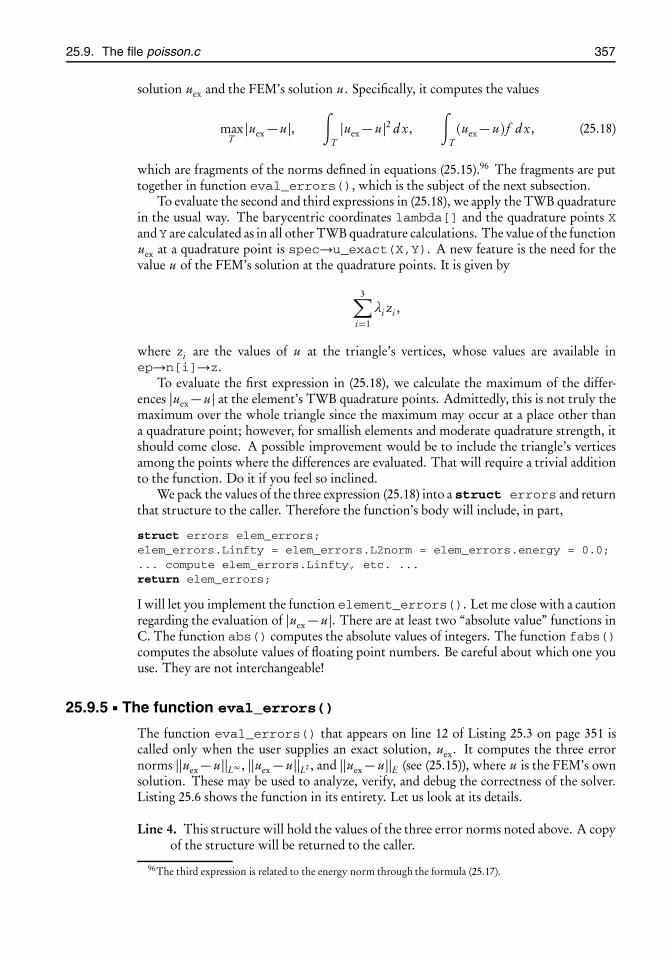
root2014/7/8page 357
�
�
�
�
�
�
�
�
25.9. The file poisson.c 357
solution uex and the FEM’s solution u. Specifically, it computes the values
maxT|uex− u|,
∫T|uex− u|2 d x,
∫T(uex− u) f d x, (25.18)
which are fragments of the norms defined in equations (25.15).96 The fragments are puttogether in function eval_errors(), which is the subject of the next subsection.
To evaluate the second and third expressions in (25.18), we apply the TWB quadraturein the usual way. The barycentric coordinates lambda[] and the quadrature points XandY are calculated as in all other TWB quadrature calculations. The value of the functionuex at a quadrature point is spec→u_exact(X,Y). A new feature is the need for thevalue u of the FEM’s solution at the quadrature points. It is given by
3∑i=1
λi zi ,
where zi are the values of u at the triangle’s vertices, whose values are available inep→n[i]→z.
To evaluate the first expression in (25.18), we calculate the maximum of the differ-ences |uex− u| at the element’s TWB quadrature points. Admittedly, this is not truly themaximum over the whole triangle since the maximum may occur at a place other thana quadrature point; however, for smallish elements and moderate quadrature strength, itshould come close. A possible improvement would be to include the triangle’s verticesamong the points where the differences are evaluated. That will require a trivial additionto the function. Do it if you feel so inclined.
We pack the values of the three expression (25.18) into a struct errors and returnthat structure to the caller. Therefore the function’s body will include, in part,
struct errors elem_errors;elem_errors.Linfty = elem_errors.L2norm = elem_errors.energy = 0.0;... compute elem_errors.Linfty, etc. ...return elem_errors;
I will let you implement the function element_errors(). Let me close with a cautionregarding the evaluation of |uex− u|. There are at least two “absolute value” functions inC. The function abs() computes the absolute values of integers. The function fabs()computes the absolute values of floating point numbers. Be careful about which one youuse. They are not interchangeable!
25.9.5 The function eval_errors()
The function eval_errors() that appears on line 12 of Listing 25.3 on page 351 iscalled only when the user supplies an exact solution, uex. It computes the three errornorms ‖uex− u‖L∞ , ‖uex− u‖L2 , and ‖uex− u‖E (see (25.15)), where u is the FEM’s ownsolution. These may be used to analyze, verify, and debug the correctness of the solver.Listing 25.6 shows the function in its entirety. Let us look at its details.
Line 4. This structure will hold the values of the three error norms noted above. A copyof the structure will be returned to the caller.
96The third expression is related to the energy norm through the formula (25.17).
root2014/7/8page 358
�
�
�
�
�
�
�
�
358 Chapter 25. Finite elements
Listing 25.6: The function eval_errors in the file poisson.c.
1 struct errors eval_errors(struct problem_spec *spec,2 struct mesh *mesh, int d)3 {4 struct errors errors;5 struct TWB_qdat *qdat = twb_qdat(&d, NULL);6 errors.Linfty = errors.L2norm = errors.energy = 0.0;7 for (int i = 0; i < mesh→nelems; i++) {8 struct elem *ep = &mesh→elems[i];9 struct errors elem_errors = element_errors(spec, qdat, ep);
10 errors.L2norm += elem_errors.L2norm;11 errors.energy += elem_errors.energy;12 if (elem_errors.Linfty > errors.Linfty)13 errors.Linfty = elem_errors.Linfty;14 }15 errors.L2norm = sqrt(errors.L2norm);16 errors.energy = sqrt(errors.energy);17 return errors;18 }
Listing 25.7: An outline of the file fem-demo.c.
1 � #include ...2 � static void do_demo(struct problem_spec *spec,3 double a, int d, char *gv_filename) ...4 � static void show_usage(char *progname) ...5 � int main(int argc, char **argv) ...
Line 6. The error norms are going to be computed one element at a time. We initializethe norms to zero in preparation for the accumulation process.
Line 9. The elem_errors is yet another instance of a struct errors. It capturesthe element-level errors returned in a call to the function element_errors().Following that call, we accumulate the returned values in errors.L2norm anderrors.energy. We also adjust errors.Linfty if the element’s error valueexceeds the previous values.
Lines 15 and 16. We take square roots in accordance with the definitions (25.15).
25.10 The file fem-demo.cThe file fem-demo.c is a driver for demonstrating our Poisson solver. Listing 25.7 shows anoutline. The functions show_usage() and main() that appear on lines 4 and 5 of thatlisting are essentially identical to those in Project TWB quadrature. The function main()expects to read two numbers, d and a, from its command-line. The first number is thestrength of the desired TWB quadrature for integrating over the elements. The secondnumber is an upper bound on the areas of the mesh’s triangles. Thus we expect argc tobe 3. If it’s not, we call show_usage() to print a brief usage message to stderr andthen exit. This is exactly what we did in Project TWB quadrature, so there is no need toelaborate.

root2014/7/8page 359
�
�
�
�
�
�
�
�
25.11. Further reading 359
Listing 25.8: The function do_demo() in the file fem-demo.c.
1 static void do_demo(struct problem_spec *spec,2 double a, int d, char *gv_filename)3 {4 struct mesh *mesh;5 mesh = make_mesh(spec, a);6 printf("nodes = %d, edges = %d, elems = %d\n",7 mesh→nnodes, mesh→nedges, mesh→nelems);8 poisson_solve(spec, mesh, d);9 if (spec→u_exact �= NULL) {
10 struct errors errors = eval_errors(spec, mesh, d);11 printf("errors: L^infty = %g, L^2 = %g, energy norm = %g\n",12 errors.Linfty, errors.L2norm, errors.energy);13 }14 plot_with_geomview_zhue(mesh, gv_filename);15 free_mesh(mesh);16 }
The function do_demo() that appears on line 2 of Listing 25.7 runs the demo for asingle problem. It receives the problem specification in the spec argument, the values ofmaximal triangle area a, TWB quadrature strength d, and a file name for writing a Ge-omview script for a three-dimensional rendering of the solution. Listing 25.8 shows theimplementation of do_demo(). It is mostly self-explanatory, so there is no need to elab-orate other than pointing out that on line 9 we check the value of spec→u_exact. If itis not NULL, then we surmise that the user has supplied an exact solution, and therefore wecall eval_errors() to compute the error norms and print them to stdout.
25.11 Further readingFor the requisite theory of PDEs you may begin with the books by Renardy andRogers [55], Mattheij, Rienstra, and ten Thije Boonkkamp [43], or Ladyzhenskaya [39],where you will find accessible introductions to the subject. The books by Quarteroni [54]and Steinbach [64] provide quick overviews of the analysis of PDEs and relate them tonumerical computations and the FEM. None of these makes for a “light reading”, how-ever; they require a moderate knowledge of mathematical analysis at an advanced under-graduate or early graduate level. I am afraid there is no easier way.
You will find more detailed (but significantly more advanced) accounts of PDEs inEvans [19], Gilbarg and Trudinger [22], and (the classic) Lions and Magenes [41]. Forthe general theory of Sobolev spaces, a specialist may consult Adams and Fournier [1]and Rudin [56]. To delve seriously into the FEM, a good understanding of the Sobolevspaces is indispensable.
All of the above focus on the regularity (that is, the differentiability properties) ofthe functions while assuming that the domain’s boundary ∂ Ω is “sufficiently smooth”.Kozlov, Maz’ya, and Rossmann [37] and Maz’ya and Rossmann [44] introduce a the-ory of weighted Sobolev spaces that extends the coverage to domains with lesser smooth-ness requirements. The articles of Soane and Rostamian [63] and Soane, Suri, and Ros-tamian [62] develop theory and finite element analysis in this setting.
As to books dealing with the analysis and implementation of the FEM, you will findexcellent introductions in Gockenbach [23], Braess [10], Szabó and Babuška [72], Brenner

root2014/7/8page 360
�
�
�
�
�
�
�
�
360 Chapter 25. Finite elements
and Scott [11], and Shapira [59]. The classic books by Ciarlet [12] and Axelsson andBarker [5] provide almost encyclopedic coverage of the analytic aspects of the FEM.
25.12 Project FEM 1Complete the program, compile, and test. Since we have an exact solution in the case ofa square domain, tabulate the error as a function of the maximal area of the triangles.
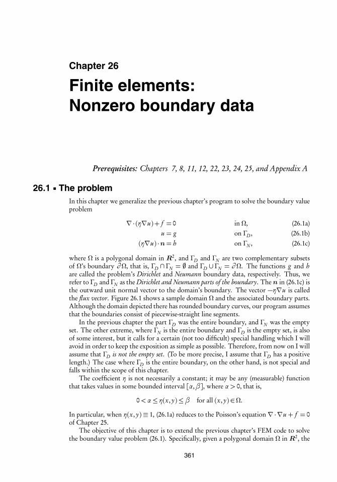
root2014/7/8page 361
�
�
�
�
�
�
�
�
Chapter 26
Finite elements:Nonzero boundary data
Prerequisites: Chapters 7, 8, 11, 12, 22, 23, 24, 25, and Appendix A
26.1 The problemIn this chapter we generalize the previous chapter’s program to solve the boundary valueproblem
∇ · (η∇u)+ f = 0 in Ω, (26.1a)u = g on ΓD , (26.1b)
(η∇u) ·n= h on ΓN , (26.1c)
where Ω is a polygonal domain in R2, and ΓD and ΓN are two complementary subsetsof Ω’s boundary ∂ Ω, that is, ΓD ∩ ΓN = " and ΓD ∪ ΓN = ∂ Ω. The functions g and hare called the problem’s Dirichlet and Neumann boundary data, respectively. Thus, werefer to ΓD and ΓN as the Dirichlet and Neumann parts of the boundary. The n in (26.1c) isthe outward unit normal vector to the domain’s boundary. The vector −η∇u is calledthe flux vector. Figure 26.1 shows a sample domain Ω and the associated boundary parts.Although the domain depicted there has rounded boundary curves, our program assumesthat the boundaries consist of piecewise-straight line segments.
In the previous chapter the part ΓD was the entire boundary, and ΓN was the emptyset. The other extreme, where ΓN is the entire boundary and ΓD is the empty set, is alsoof some interest, but it calls for a certain (not too difficult) special handling which I willavoid in order to keep the exposition as simple as possible. Therefore, from now on I willassume that ΓD is not the empty set. (To be more precise, I assume that ΓD has a positivelength.) The case where ΓD is the entire boundary, on the other hand, is not special andfalls within the scope of this chapter.
The coefficient η is not necessarily a constant; it may be any (measurable) functionthat takes values in some bounded interval [α,β], where α > 0, that is,
0<α≤ η(x, y)≤β for all (x, y) ∈Ω.
In particular, when η(x, y) ≡ 1, (26.1a) reduces to the Poisson’s equation ∇ ·∇u + f = 0of Chapter 25.
The objective of this chapter is to extend the previous chapter’s FEM code to solvethe boundary value problem (26.1). Specifically, given a polygonal domain Ω in R2, the
361
root2014/7/8page 362
�
�
�
�
�
�
�
�
362 Chapter 26. Finite elements: Nonzero boundary data
n
η∇u
ΓN
ΓD
Ω
Figure 26.1: A sample two-dimensional domain Ω with a hole. The boundary part ΓD ,drawn in solid lines, consists of two curves. The boundary part ΓN is drawnin a dashed line. The outward unit normal n and the flux vector η∇u areshown at an arbitrary point on ΓN . Our FEM implementation assumesthat the domain is polygonal; therefore you should imagine the boundarycurves as piecewise-straight line segments.
boundary parts ΓD and ΓN , and the functions η, f , g , and h, the program will find an ar-bitrarily close approximation to the function u that satisfies the three equations in (26.1).
Remark 26.1. The Neumann boundary condition (26.1c) is equivalent to η∂ u/∂ n = h,that is, ∂ u/∂ n = h/η, where ∂ u/∂ n is the directional derivative of u in the directionof the outward normal n. It is likely that you will see the Neumann boundary conditionexpressed in this form in some books and articles.
Remark 26.2. If the boundary value problem models a diffusion process in a materialthat occupies the domain Ω, then the coefficient η is the material’s diffusivity. In the caseof heat conduction, η is the material’s conductivity. In general, the physical meaning of ηdepends on the application. If η is constant throughout Ω, then the material is said to behomogeneous; otherwise it is inhomogeneous.
Remark 26.3. This chapter’s theory and implementation may be generalized in quite astraightforward way to the equation
∇ · (A∇u)+ f = 0, (26.2)
where A =�Ai j (x, y)
�is a 2× 2 matrix at any (x, y) ∈ Ω. Equation (26.1a) is a special
case of (26.2) where A(x, y) = η(x, y)I , where I is the 2× 2 identity matrix. If A(x, y) is amultiple of identity, the material is said to be isotropic at (x, y); otherwise it is anisotropic.
26.2 The weak formulationIn the weak formulation of the boundary value problem in Chapter 25, I steered awayfrom technical jargon and couched the statements in a somewhat vague and “soft” termi-nology. In this chapter I will take the opposite approach: I will present the weak formu-lation properly in terms of Sobolev spaces. Even if you are not familiar with the theoryof Sobolev spaces, you should be able to read through this material and get the gist of itto an extent that enables you to proceed with the implementation of the project.
In what follows, H 1(Ω) is the Sobolev space of functions defined onΩwhich are squareintegrable and whose first order generalized derivatives are also square integrable. Let ΓDand ΓN be the boundary parts introduced in the previous section. We write H 1
g ,ΓD(Ω) for

root2014/7/8page 363
�
�
�
�
�
�
�
�
26.2. The weak formulation 363
the subset of functions in H 1(Ω) that take on (in the sense of traces) the value g on the ΓDpart of the boundary and H 1
0,ΓD(Ω) for the subset of functions in H 1(Ω) that vanish (i.e.,
take on the zero value) on ΓD . Let us note that H 1g ,ΓD(Ω) is an affine space in H 1(Ω) if g is
nonzero. On the other hand, H 10,ΓD(Ω) is a proper subspace of H 1(Ω).
Let u ∈ H 1g ,ΓD(Ω) be the solution of the boundary value problem (26.1), and let v ∈
H 10,ΓD(Ω) be an arbitrary function. Multiply (26.1a) by v and integrate over Ω,∫
Ω
v div(η∇u)d x +∫Ω
f v d x = 0;
then apply Green’s identity ((25.4) on page 339) to the first integral to get∫∂ Ω
v η∇u ·nda−∫Ω
η∇u ·∇v d x +∫Ω
f v d x = 0.
Split the boundary integral into the sum of integrals over ΓD and ΓN . The former is zerosince v = 0 on ΓD . The latter may be simplified by applying (26.1c). After rearrangingthe terms we get the identity∫
Ω
η∇u ·∇v d x =∫Ω
f v d x +∫ΓN
hv da,
which holds for all v in H 10,ΓD(Ω). Conversely, if the above holds for a u ∈ H 1
g ,ΓD(Ω) and all
v in H 10,ΓD(Ω), one may deduce that u is a solution of the original boundary value problem.
(The derivatives should be interpreted as generalized derivatives, but that technical issueis beyond the scope of this book.) This leads to the following weak formulation of theboundary value problem:
Find u ∈ H 1g ,ΓD(Ω) such that∫
Ω
η∇u ·∇v d x =∫Ω
f v d x +∫ΓN
hv da for all v ∈H 10,ΓD(Ω). (26.3)
Remark 26.4. In the special case when h is identically zero on ΓN , the weak formula-tion (26.3) reduces to the following:
Find u ∈ H 1g ,ΓD(Ω) such that∫Ω
η∇u ·∇v d x =∫Ω
f v d x for all v ∈ H 10,ΓD(Ω).
You may note that there is no explicit reference to a Neumann boundary condition here.In a sense, omitting h in the weak formulation is equivalent to taking h as identically zero.Because of this, a zero Neumann boundary condition is also known as a natural boundarycondition.

root2014/7/8page 364
�
�
�
�
�
�
�
�
364 Chapter 26. Finite elements: Nonzero boundary data
26.3 The Galerkin approximationFollowing the ideas of Chapter 25, we triangulate Ω with a quasi-uniform mesh whosefineness is determined by a parameter a that specifies an upper bound on triangle areas.The number m of the mesh’s nodes will increase as a decreases. Recall the construction,in Section 25.4, of the function space Vm whose basis consisted of the pyramidal functionsdepicted in Figure 25.1 on page 342. The preliminary construction in that section placedone pyramid at each interior node of the mesh. Boundary nodes were excluded since wewere dealing with zero Dirichlet data. In the present chapter, the space Vm is constructedin the same way; however, there is a pyramidal basis function at every node, includingthe boundary nodes, since we are dealing with general boundary conditions. Of course,those parts of the pyramids that lie outside the domain Ω are immaterial to our purposes.It may be shown (see, e.g., [12]) that Vm is a linear subspace of H 1(Ω), and that a functionin H 1(Ω) may be approximated with a function in Vm with any desired accuracy if m issufficiently large.
Let us write # = {1,2, . . . , m} for the index set of the triangulation’s nodes, and let ussplit # into the disjoint union # = �# ∪#D , where #D is the subset of # correspondingto the vertices that fall on the part ΓD of the domain’s boundary, and �# is the rest of # .We will write gi for the values of the Dirichlet data g at the point vi when i ∈ #D .
Here we introduce the finite-dimensional counterparts of the spaces H 10,ΓD(Ω) and
H 1g ,ΓD(Ω) that enter the weak formulation (26.3):
V0,m =�∑
i∈ �#ci vi : all possible choices of coefficients ci
= span{vi : i ∈ �# },
Vg ,m =�∑
i∈ �#ci vi +
∑i∈#D
gi vi : all possible choices of coefficients ci
.
Then the Galerkin approximation of the weak formulation (26.3) takes the followingform:
Find um ∈Vg ,m such that∫Ω
η∇um ·∇v d x =∫Ω
f v d x +∫ΓN
hv da for all v ∈V0,m ,
or equivalently, the following:
Find {c j } j∈ �# such that∫Ω
η∇*∑
j∈ �#c j v j +
∑j∈#D
gj v j
+·∇vi d x =
∫Ω
f vi d x +∫ΓN
hvi da for all i ∈ �# .
(26.4)
The formulation (26.4) is a linear system of �m equations in the �m unknowns c j , where
�m is the cardinality of the set �# . In analogy with (25.12) (page 341) let us write thisas �Kc = �b . The system may be assembled and solved, in principle, along the lines de-veloped for the simpler case of Chapter 25. In practice, however, the following slightreformulation of (26.4) will help to streamline the program’s algorithm. The purpose of

root2014/7/8page 365
�
�
�
�
�
�
�
�
26.3. The Galerkin approximation 365
the reformulation is to remove references to the index sets �# and #D in (26.4) in favor ofthe larger but simpler index set # . Toward that end, we express
um =∑j∈ �#
c j v j +∑j∈#D
gj v j =∑j∈#
c j v j , (26.5)
thus extending the count of the unknowns ci from �m to m. At the same time, we appendm− �m equations of the type c j = gj , j ∈ #D , to the previous system, thus arriving at asystem Kc = b of m equations in m unknowns with the following general structure:⎛⎜⎜⎜⎜⎜⎜⎜⎜⎜⎝
k11 k12 · · · k1 j · · · k1mk21 k22 · · · k2 j · · · k2m...0 0 · · · 1 · · · 0...
km1 km2 · · · km j · · · kmm
⎞⎟⎟⎟⎟⎟⎟⎟⎟⎟⎠
⎛⎜⎜⎜⎜⎜⎜⎜⎜⎜⎝
c1c2...
c j...
cm
⎞⎟⎟⎟⎟⎟⎟⎟⎟⎟⎠=
⎛⎜⎜⎜⎜⎜⎜⎜⎜⎜⎝
b1b2...
gj...
bm
⎞⎟⎟⎟⎟⎟⎟⎟⎟⎟⎠. (26.6)
Row j expresses the constraint c j = gj , assuming that the index j is in the set#D . There isone such row for every vertex that falls on ΓD . We may exploit that row’s simple structureto eliminate the rest of the entries in column j , as in⎛⎜⎜⎜⎜⎜⎜⎜⎜⎝
k11 k12 · · · 0 · · · k1mk21 k22 · · · 0 · · · k2m...0 0 · · · 1 · · · 0...
km1 km2 · · · 0 · · · kmm
⎞⎟⎟⎟⎟⎟⎟⎟⎟⎠
⎛⎜⎜⎜⎜⎜⎜⎜⎜⎜⎝
c1c2...
c j...
cm
⎞⎟⎟⎟⎟⎟⎟⎟⎟⎟⎠=
⎛⎜⎜⎜⎜⎜⎜⎜⎜⎜⎝
b1− gj k1 jb2− gj k2 j
...gj...
bm − gj km j
⎞⎟⎟⎟⎟⎟⎟⎟⎟⎟⎠. (26.7)
The elimination that takes (26.6) to (26.7) is by no means essential, but it helps to makethe sparse coefficient matrix K more sparse and thus increase UMFPACK’s efficiency.
In view of the weak formulation in (26.4) and the compact form in (26.5) of um , theentries Ki j of the system stiffness matrix K are given by
Ki j =∫Ω
η∇vi ·∇vj d x d y.
As we saw in Chapter 25, however, there is little use for such a “node-based” formula. The“element-based” approach is easier to implement. Thus, we introduce the 3× 3 elementstiffness matrix k on the triangle T , given by
ki j =∫
Tη∇φi ·∇φ j d x d y, i , j = 1,2,3,
where φi (x, y) = λi is the nodal shape function corresponding to the vertex i of thetriangle T . Here (λ1,λ2,λ3) are the barycentric coordinates of the point (x, y).
Since a shape function is a first degree polynomial, then∇φi is a constant vector, andtherefore it may be pulled out of the integration sign. Applying (A.10) (on page 379), theexpression for ki j reduces to
ki j =�
1
4|T |2 ei ·e j
��∫Tηd x d y
�. (26.8)

root2014/7/8page 366
�
�
�
�
�
�
�
�
366 Chapter 26. Finite elements: Nonzero boundary data
In particular, when η≡ 1, the integral equals the area |T | of the triangle; therefore (26.8)reduces to Chapter 25’s (25.14).
Remark 26.5. Rearranging the expression (26.8) into
ki j =�
1
4|T |ei ·e j
��1
|T |∫
Tηd x d y
�(26.9)
we see that the element stiffness matrix is exactly the previous chapter’s element stiffnessmatrix multiplied by the average of η over the element. This observation should help youwith adapting your previous code to the current situation.
26.4 The programThe implementation of the FEM solver for the boundary value problem (26.1) amountsto making small changes to the solver of Chapter 25. I assume that you have read thatchapter and implemented its program. In this chapter I will focus only on the differences.Here is what my directory looks like:
$ cd fem2$ ls -FMakefile mesh.h@ [email protected]@ plot-with-geomview.c@ [email protected] plot-with-geomview.h@ [email protected]@ poisson.c [email protected]@ poisson.h [email protected]@ problem-spec.c
The file problem-spec.h remains unchanged from that in Project Triangulate of Chap-ter 23; therefore a symbolic link to that file will do. The file problem-spec.c is substantiallydifferent; make a copy from Chapter 25, and edit. In problem-spec.c we define four prob-lems, called square1(), square2(), square3(), square4(), each correspondingto a boundary value problem on the unit square Ω= (0,1)× (0,1). Figures 26.2 and 26.3provide all the necessary details. Problems square1() andsquare2() test your code’sability to apply nonzero Dirichlet and Neumann boundary data, respectively. Theyshare the same forcing function f and exact solution uex. Problem square3() testsyour code’s ability to handle inhomogeneous media, that is, nonconstant η. Problemsquare4(), for which no exact solution is available, demonstrates a case where one sideof the square is split into two intervals with different boundary conditions. Listing 26.1shows the transcript of a sample session.
When an exact solution is available, the program computes and prints the errors in theL∞ and L2 norms. We don’t compute the error in the energy norm since it requires aneffort beyond the scope of this chapter. The formula (25.17) (page 347) is not applicablesince the zero Dirichlet data was used in an essential way in its derivation.
26.5 The file problem-spec.[ch]The file problem-spec.h remains unchanged from that in Project Triangulate of Chapter 23;therefore a symbolic link to that file will do. The file problem-spec.c defines the fourboundary value problems depicted in Figures 26.2 and 26.3. The domain specificationsare minor variations on the previous chapter’s square domain. The novel element here

root2014/7/8page 367
�
�
�
�
�
�
�
�
26.5. The file problem-spec.[ch] 367
square1()
η≡ 1
g = 4x(1− x)
g = 0g = 0
g = 0
square2()
η≡ 1
h = 20x(1− x)
g = 0g = 0
g = 0
uex = 4x(1− x)(1− y)(1− 4y)f =−32x(1− x)+ 8(1− y)(1− 4y)
Figure 26.2: These figures declare two boundary value problems on the domain Ω =(0,1)× (0,1). The version on the left, square1(), has Dirichlet data allaround. The version on the right, square2(), has Neumann data on thebottom edge and Dirichlet data on the other three edges. In both cases thecoefficient η is identically equal to 1 throughout, and the forcing functionf and the exact solution uex are as given.
square3()
η= 1+ x2 + y2g = uexg = uex
g = uex
g = uex
f = 16(x − 1/8)2+ 16(y − 1/8)2+ 15/2
uex = 1− 2(x − 1/2)2− 2(y − 1/2)2
square4()
η≡ 1
g = 1 h = 0
h = 0h = 0
g = 0
f ≡ 0
Figure 26.3: These figures declare two boundary value problems on the domain Ω =(0,1)× (0,1). The version on the left, square3(), has Dirichlet data allaround which is “inherited” from the exact solution uex. The coefficient ηis nonconstant. The version on the right, square4(), has mixed Dirich-let and Neumann data on the various parts of the boundary. The coeffi-cient η is identically equal to 1 throughout, and the forcing function f iszero.
is the care that goes into specifying the boundary condition types. Listing 26.2 showsthe definition of the domain labeled square2() in Figure 26.2. We see that the bottomside is given the FEM_BC_NEUMANN attribute, while the other three sides are of the typeFEM_BC_DIRICHLET. All four vertices, however, are of the typeFEM_BC_DIRICHLETsince the boundary values are prescribed on all four.
The functions square_g() and square_h() that appear in that listing may bedefined in a variety of ways. Here is one possibility:

root2014/7/8page 368
�
�
�
�
�
�
�
�
368 Chapter 26. Finite elements: Nonzero boundary data
Listing 26.1: The transcript of a sample session with this chapter’s program.
$ ./fem-demoUsage: ./fem-demo d a
d = the TWB quadrature strengtha = maximal triangle area
$ ./fem-demo 10 0.002domain is square1:nodes = 428, edges = 1217, elems = 790system stiffness matrix is 428x428 (=183184) has 2862 nonzero entrieserrors: L^infty = 0.00977244, L^2 = 0.0022182geomview output written to file square1.gv
domain is square2:nodes = 428, edges = 1217, elems = 790system stiffness matrix is 428x428 (=183184) has 2862 nonzero entrieserrors: L^infty = 0.0111535, L^2 = 0.00219217geomview output written to file square2.gv
domain is square3:nodes = 428, edges = 1217, elems = 790system stiffness matrix is 428x428 (=183184) has 2862 nonzero entrieserrors: L^infty = 0.00378925, L^2 = 0.00196628geomview output written to file square3.gv
domain is square4:nodes = 433, edges = 1232, elems = 800system stiffness matrix is 433x433 (=187489) has 2897 nonzero entriesgeomview output written to file square4.gv
double square_g(double x, double y){
return 0.0}
We need not be concerned that square_g() returns incorrect values on square2()’sbottom edge (where the solution is nonzero) since g is never evaluated on that edge; it isevaluated only on the boundary parts of the FEM_BC_DIRICHLET type.
Another alternative, taking advantage of the availability of the exact solution, wouldbe
double square_g(double x, double y){
return square_u_exact(x, y);}
since obviously the exact solution satisfies the boundary condition. The second alterna-tive has a slight advantage over the first one since it applies to both the square1() andsquare2() problems of Figure 26.2.
For the same reasons, the function square_h() that produces the Neumann datafor square2() may be given simply as

root2014/7/8page 369
�
�
�
�
�
�
�
�
26.6. The file poisson.c 369
Listing 26.2: The specification in the file problem-spec.c of the domain corresponding to the bound-ary value problem square2() in Figure 26.2.
1 struct problem_spec *square2(void)2 {3 static struct problem_spec_point points[] = {4 { 0, 0.0, 0.0, FEM_BC_DIRICHLET },5 { 1, 1.0, 0.0, FEM_BC_DIRICHLET },6 { 2, 1.0, 1.0, FEM_BC_DIRICHLET },7 { 3, 0.0, 1.0, FEM_BC_DIRICHLET },8 };9 static struct problem_spec_segment segments[] = {
10 { 0, 0, 1, FEM_BC_NEUMANN },11 { 1, 1, 2, FEM_BC_DIRICHLET },12 { 2, 2, 3, FEM_BC_DIRICHLET },13 { 3, 3, 0, FEM_BC_DIRICHLET },14 };15 static struct problem_spec spec = { // C99-style initialization!16 .points = points,17 .npoints = (sizeof points)/(sizeof points[0]),18 .segments = segments,19 .nsegments = (sizeof segments)/(sizeof segments[0]),20 .holes = NULL,21 .nholes = 0,22 .f = square_f,23 .g = square_g,24 .h = square_h,25 .eta = one,26 .u_exact = square_u_exact,27 };28 printf("domain is square2:\n");29 return &spec;30 }
double square_h(double x, double y){
return 20*x*(1-x);}
Again, we need not be concerned that it does not represent the correct Neumann data onedges other than the bottom; it is evaluated only on the bottom edge.
The domain specification of the problem square4() in Figure 26.3 is slightly differ-ent than the others since the bottom edge needs to be split into two distinct zones withFEM_BC_DIRICHLET and FEM_BC_NEUMANN attributes. To achieve that, define thesquare as a polygon with five vertices and five segments—the bottom edge consisting oftwo segments—and then specify the boundary types in the usual way.
26.6 The file poisson.cThis chapter’s poisson.c is a slight modification of the previous chapter’s. Listing 26.3provides an outline. The function error_and_exit() remains unchanged. The func-tionselement_errors() and eval_errors() are curtailed versions of the previous
root2014/7/8page 370
�
�
�
�
�
�
�
�
370 Chapter 26. Finite elements: Nonzero boundary data
Listing 26.3: An outline of the file poisson.c.
1 #include ...2 � static void error_and_exit(int status,3 const char *file, int line) ...4 � static void apply_dirichlet_bc(struct elem *ep,5 double (*g)(double x, double y), double k[3][4]) ...6 � static void apply_neumann_bc(struct elem *ep,7 double (*h)(double x, double y),8 double k[3][4], struct Gauss_qdat *gqdat) ...9 � static void compute_element_stiffness(
10 struct elem *ep, struct TWB_qdat *qdat,11 double (*f)(double x, double y),12 double (*eta)(double x, double y),13 double k[3][4]) ...14 � void poisson_solve(struct problem_spec *spec,15 struct mesh *mesh, int d) ...16 � static struct errors element_errors(struct problem_spec *spec,17 struct TWB_qdat *qdat, struct elem *ep) ...18 � struct errors eval_errors(struct problem_spec *spec,19 struct mesh *mesh, int d)
code; they compute the error in the L2 and L∞ norms only. Computing the energy normrequires extra work, so we will not implement it. We will review the remaining functionsin the following subsections.
26.6.1 The function compute_element_stiffness()
The function compute_element_stiffness() that appears on line 9 of Listing 26.3requires only small adjustments relative to the previous chapter’s function of the samename. First, we calculate the 12 entries of the 3× 4 element stiffness matrix exactly as be-fore. Next, in view of Remark 26.5 on page 366, we multiply the 3× 3 part of the matrix(i.e., everything other than the rightmost column) by the average of η over the element.Since compute_element_stiffness() has already set up the TWB quadrature ma-chinery for computing the fourth column of the element stiffness matrix, we may pig-gyback on that machinery to compute the integral of η. Very little extra code is neededhere.
26.6.2 Applying the Neumann boundary data
According to the formulation (26.4), the contributions of the problem’s force function, f ,and the Neumann boundary data, h, appear as the sum
∫Ω
f vi d x +∫ΓN
hvi da. At theelement level, the first integral deposits entries in the fourth column of the 3× 4 elementstiffness matrix, just as it did in the previous chapter’s program. The second integraldeposits additional material in that column. The deposited values accumulate, reflectingthe fact that the two integrals are being added.
To determine the contribution of the second integral at the element level, let us con-sider an element with vertices vi , v j , vk (in counterclockwise order) whose edge i lieson the ΓN part of the boundary. Recall that edge i lies opposite the vertex i ; thereforeit extends from the vertex v j to the vertex vk . Figure 26.4 depicts a representative case.

root2014/7/8page 371
�
�
�
�
�
�
�
�
26.6. The file poisson.c 371
v j −ei → FEM_BC_NEUMANN vk
−ej→
vi← ek−
the basis function vj
the basis function vk
Figure 26.4: The diagram shows an element with vertices vi , v j , vk and edge vectorsei , e j , ek . The edge ei lies on the domain’s boundary and has a boundaryof type FEM_BC_NEUMANN. Parts of the basis functions vj (centered atnode v j ) and vk (centered at node vk ) are shown. The trace of the basisfunction vj on the edge ei is a linear function that goes from 1 at the vertexv j to 0 at the vertex vk . Similarly, the trace of the basis function vk on theedge ei is a linear function that goes from 1 at the vertex vk to 0 at thevertex v j .
Additionally, the figure shows the fragments of the basis functions (pyramids) vj and vkcentered at the vertices v j and vk . We see in that figure that along the edge ei , the ba-sis function vj drops linearly from the value 1 at the endpoint vj to the value 0 at theendpoint vk . To obtain an equation for that function, let us parametrize the edge ei as in
edge ei :1
2(1− ξ )v j +
1
2(1+ ξ )vk , −1≤ ξ ≤ 1.
Thus, ξ = −1 puts us at v j , and ξ = 1 puts us at vk . Then the restriction of the basisfunction vj to the edge ei is the function 1
2 (1− ξ ) since it takes on the value 1 at theendpoint vj and the value 0 at the endpoint vk . Consequently, the integral
∫ΓN
hvj daalong the edge ei takes the form
L2
∫ 1
−1
1
2(1− ξ ) h
�1
2(1− ξ )v j +
1
2(1+ ξ )vk
�dξ , (26.10a)
where L is the actual length of the edge ei , that is, L= ‖vk−v j ‖. The L/2 factor accountsfor the change of the domain of integration from the edge ei whose length is L to theparameter space (−1,1) whose length is 2. (See equations (22.2) on page 291 for a clearerexplanation.) The value of this integral is deposited in (that is, added to) the ( j , 3) entryof the element stiffness matrix since it represents the
∫ΓN
hvj da integral.This takes care of half of the required computation. We also need to evaluate the
integral∫ΓN
hvk da along the edge ei . You should have no difficulty in seeing that it is

root2014/7/8page 372
�
�
�
�
�
�
�
�
372 Chapter 26. Finite elements: Nonzero boundary data
Listing 26.4: An outline of the function apply_neumann_bc() in the file poisson.c.
1 static void apply_neumann_bc(struct elem *ep,2 double (*h)(double x, double y),3 double k[3][4], struct Gauss_qdat *gqdat)4 {5 for (int i = 0; i < 3; i++) // scan the element’s edges6 if (ep→e[i]→bc == FEM_BC_NEUMANN) {7 � let (x1,y1) be the coords of one end of edge i8 � let (x2,y2) be the coords of the other end of edge i9 � compute the length L of the edge
10 double sum1 = 0.0; // the integral in (26.10a)11 double sum2 = 0.0; // the integral in (26.10b)12 while (gqdat→w �= -1) { // do Gaussian quadrature13 � ...14 gqdat++;15 }16 k[(i+1)%3][3] += L/2*sum1; // deposit the compted values in17 k[(i+2)%3][3] += L/2*sum2; // the element stiffness matrix18 }19 }
given by
L2
∫ 1
−1
1
2(1+ ξ ) h
�1
2(1− ξ )v j +
1
2(1+ ξ )vk
�dξ . (26.10b)
The value of this integral is deposited in (that is, added to) the (k , 3) entry of the elementstiffness matrix since it represents the
∫ΓN
hvk da integral.The function apply_neumann_bc() that appears on line 6 of Listing 26.3 is re-
sponsible for evaluating these two integrals via Gaussian quadrature and depositing theirvalues into the element stiffness matrix. Listing 26.4 gives an outline. Note that the in-dices of the vertices v j and vk appear as (i+1)%3 and (i+2)%3, as usual.
26.6.3 Applying the Dirichlet boundary data
The function apply_dirichlet_bc() that appears on line 4 in Listing 26.3 gener-alizes the previous chapter’s enforce_zero_dirichlet_bc() function to nonzeroDirichlet data. It receives an element’s 3 × 4 stiffness matrix k and modifies it to en-force the prescribed Dirichlet data in accordance with the algorithm described in formu-las (26.6) and (26.7). Specifically, if the element’s vertex i (where i is one of 0,1,2) is of typeFEM_BC_DIRICHLET, it zeros the k’s row i , replaces ki3 with the prescribed boundaryvalue, gi , and sets kii to 1. The middle block of the diagram below illustrates this withi = 1:
k00 k01 k02 k03
k10 k11 k12 k13
k20 k21 k22 k23
k00 k02 k03
k20 k22 k23
0 1 0 g1
k01
k21
=⇒k00 k02 k03− g1k01
k20 k22 k23− g1k21
0 1 0 g1
0
0
=⇒

root2014/7/8page 373
�
�
�
�
�
�
�
�
26.7. Project FEM 2 373
As was noted in connection with (26.7), we may use the modified row to eliminate the en-tries in column i through row operations and arrive at the matrix depicted at the right endof the diagram above. The elimination is not necessary and does not affect the problem’ssolution. However, it results in a sparser system stiffness matrix which is advantageousin connection with UMFPACK.
26.6.4 The order of the application of the boundary conditions
The rest of the file poisson.c is pretty much the same as Chapter 25’s version. I wish topoint out one subtle issue that you should take into account when making the transitionto this chapter’s version.
Let us look at Listing 25.4 of the function poisson_solve() on page 354.On line 30 we call enforce_zero_dirichlet_bc() to enforce the bound-ary conditions. In the current chapter that line will be replaced with a call toapply_neumann_bc() to process the problem’s Neumann boundary data and thena call to apply_dirichlet_bc() to process the problem’s Dirichlet boundary data.The order of the calls is absolutely essential! To see the reason why, consider a boundarynode which is at the transition point between a Dirichlet edge and a Neumann edge. Theapplication of the Neumann boundary condition adds the integrals (26.10) to that node’s“force” term in the system stiffness matrix. The application of the Dirichlet boundarycondition resets that force term to the prescribed boundary value. If the boundary condi-tions were applied, incorrectly, in the reversed order, then the value set by the Dirichletdata would be overwritten by the integrals of the Neumann data.
26.7 Project FEM 2Complete the program, compile, and test with the four boundary value problems definedin Section 26.4. Compare your results to the transcript shown in that section and thegraphs shown in Figure 26.5.

root2014/7/8page 374
�
�
�
�
�
�
�
�
374 Chapter 26. Finite elements: Nonzero boundary data
square1(), square2() square3()
square4() (view 1) square4() (view 2)
Figure 26.5: The graphs of the solutions of the four boundary value prob-lems defined in Section 26.4 as obtained through the command./fem-demo 10 0.005 and rendered in Geomview. The problemssquare1() and square2() have identical solutions. Two views of thesolution of problem square4() are shown.

root2014/7/8page 375
�
�
�
�
�
�
�
�
Appendix A
Barycentric coordinates
A.1 Barycentric coordinatesFigure A.1 shows the equilateral triangle% formed by the part of the plane λ1+λ2+λ3 =1 that lies in the positive octant in the (λ1,λ2,λ3) Cartesian coordinate system. It alsoshows a generic triangle with verticesv1, v2, v3 in the (x1, x2)Cartesian coordinate system.For reasons that will become clear shortly, we assume that the triangle T has a nonemptyinterior and that its vertices are enumerated in counterclockwise order. The equation
x= λ1v1+λ2v2+λ3v3 (A.1)
establishes a bijection, i.e., a one-to-one and onto mapping, between the triangle % inthe three-dimensional (λ1,λ2,λ3) space and the triangle T in the two-dimensional (x1, x2)space. In particular, the vertices (1,0,0), (0,1,0), and (0,0,1) of % map to the verticesv1, v2, and v3 of T , respectively. The boundary of % maps onto the boundary of T ,and the interior of % maps onto the interior of T . To every point λ = (λ1,λ2,λ3) ∈ %there corresponds a unique point x = (x1, x2) ∈ T , and conversely, to every point x =(x1, x2) ∈ T there corresponds a unique point λ= (λ1,λ2,λ3) ∈ % . The triplet (λ1,λ2,λ3)associated with the point of x ∈ T is called that point’s barycentric coordinates. Figure A.1illustrates the geometry.
To explore further, let us introduce the notation
v1 =�
v11v12
�, v2 =
�v21v22
�, v3 =
�v31v32
�,
whereby (A.1) takes the form�x1x2
�=�
v11 v21 v31v12 v22 v32
�⎛⎝λ1λ2λ3
⎞⎠ , where λ1+λ2+λ3 = 1,
or equivalently, ⎛⎝x1x21
⎞⎠=⎛⎝v11 v21 v31
v12 v22 v321 1 1
⎞⎠⎛⎝λ1λ2λ3
⎞⎠ . (A.2)
Equation (A.1), or its expanded form (A.2), carry us from the barycentric coordinates(λ1,λ2,λ3) to the Cartesian coordinates (x1, x2). The mapping in the reverse direction is
375

root2014/7/8page 376
�
�
�
�
�
�
�
�
376 Appendix A. Barycentric coordinates
λ1
λ2
λ3
11
1
λ1+λ2+λ3 = 1
%x1
x2
v1v2
v3
T
e3
e1e2
(λ1,λ2,λ3)→ (x1, x2)
Figure A.1: The equilateral triangle % in the λ1-λ2-λ3 coordinate system is mapped tothe triangle T in the x-y coordinate system. The edge vectors e1, e2, e3 aredefined in (A.3).
obtained by inverting the coefficient matrix. The outcome is best expressed in terms ofthe triangle T ’s edge vectors
e1 =�
e11e12
�, e2 =
�e21e22
�, e3 =
�e31e32
�,
which are defined through
e1 = v3−v2, e2 = v1−v3, e3 = v2−v1 (A.3)
and shown graphically in Figure A.1. Upon inverting the mapping (A.2) we obtain⎛⎝λ1λ2λ3
⎞⎠= 1
e11e22− e21e12
⎛⎝−e12 e11 (v21v32− v31v22)−e22 e21 (v31v12− v11v32)−e32 e31 (v11v22− v21v12)
⎞⎠⎛⎝x1x21
⎞⎠ . (A.4)
Remark A.1. We recognize the expression in the denominator as the sole nonzero com-ponent of the cross product e1 × e2—here we are thinking of the vectors e1 and e2 asembedded in the three-dimensional space—therefore it equals the area of the parallelo-gram formed by those two vectors, that is to say, twice the area of the triangle T . Ourassumptions that the triangle T has nonempty interior and that its vertices are orderedcounterclockwise imply that e11e22− e21e12 is positive.
Since the triangle’s area can be expressed equally well in terms of the cross productse2×e3 or e3×e1, any of the following expressions may be used to compute the area:
|T |= 1
2(e11e22− e21e12) =
1
2(e21e32− e31e22) =
1
2(e31e12− e11e32). (A.5)
Remark A.2. For future reference, let us note that (A.4) is equivalent to⎛⎝λ1λ2λ3
⎞⎠= 1
2|T |
⎛⎝−e12 e11−e22 e21−e32 e31
⎞⎠�x1x2
�+
1
2|T |
⎛⎝v21v32− v31v22v31v12− v11v32v11v22− v21v12
⎞⎠ . (A.6)
Thus, by letting
B =1
2|T |
⎛⎝−e12 e11−e22 e21−e32 e31
⎞⎠ , b=1
2|T |
⎛⎝v21v32− v31v22v31v12− v11v32v11v22− v21v12
⎞⎠ , (A.7)

root2014/7/8page 377
�
�
�
�
�
�
�
�
A.2. Calculus on a triangle 377
v1 v2
v3
λ1 =
0.00
λ1 =
0.25
λ1 =
0.50
λ1 =
0.75
λ1 =
1.00
λ3 = 0.00
λ3 = 0.25
λ3 = 0.50
λ3 = 0.75
λ3 = 1.00
λ 2=
0.00
λ 2=
0.25
λ 2=
0.50
λ 2=
0.75
λ 2=
1.00
Figure A.2: The barycentric coordinate lines are parallel to the triangle’s sides. Thecoordinate lines λi = constant are parallel to the edge opposite the vertex i .
and λ= (λ1,λ2,λ3), (A.6) takes on the compact form
λ= Bx+ b. (A.8)
In conclusion, (A.1) maps from barycentric coordinates to Cartesian, and (A.8) mapsfrom Cartesian to barycentric.
A.1.1 The barycentric coordinate lines
If you are new to the concept of barycentric coordinates, it would be worthwhile to spenda few minutes studying the diagram in Figure A.2, which shows the barycentric coordi-nate lines. Note, for instance, that the lines λi = constant are parallel to the edge oppositethe vertex vi . In particular, the horizontal line marked λ3 = 0.25 is parallel to the trian-gle’s base. When we move along that line from the triangle’s left edge to the right edge, theλ2 coordinate varies from 0 to 0.75, and the λ1 coordinate varies from 0.75 to 0. Duringthat motion, and indeed anywhere in the triangle, we have λ1+λ2+λ3 = 1.
A.1.2 The barycentric coordinates under a linear map
Consider a linear mapping L of the x1-x2 plane into itself. Suppose L takes the triangle Twith vertices v1, v2, v3 to a triangle T ′ with vertices v′1, v′2, v′3, as illustrated in Figure A.3.Consider a point x ∈ T specified through its barycentric coordinates (λ1,λ2,λ3), that is,x= λ1v1+λ2v2+λ3v3. Let x′ = Lx ∈ T ′. Then
x′ = Lx= L(λ1v1+λ2v2+λ3v3) = λ1Lv1+λ2Lv2+λ3Lv3
= λ1v′1+λ2v
′2+λ3v
′3.
We see that the barycentric coordinates of x′ relative to T ′ are also (λ1,λ2,λ3). Thatis, barycentric coordinates are preserved under linear maps. This is a crucially importantproperty in applications to integration on triangles.
A.2 Calculus on a triangleConsider the triangles % and T shown in Figure A.1. As before, we assume that thevertices v1, v2, v3 are enumerated in counterclockwise order, and that T has positive

root2014/7/8page 378
�
�
�
�
�
�
�
�
378 Appendix A. Barycentric coordinates
x1
x2
v1 v2
v3
xT
v′1
v′2
v′3
x′T ′L
Figure A.3: The linear transformation L maps the triangle T to T ′. The point x and itsimage x′ = Lx have the same barycentric coordinates relative to T and T ′.
x1
x2
x3
v1 v2
v3
height = 1
Figure A.4: The graph of the function f (x) = f�λ(x)
, where f (λ) = λ1.
area, that is, |T | > 0. We write x as a shorthand for (x1, x2) and λ as a shorthand for(λ1,λ2,λ3). In light of the one-to-one relationship between the Cartesian coordinates xand the barycentric coordinates λ, we write x(λ)when we wish to emphasize the depen-dence of x on λ. Similarly, we write λ(x) to emphasize the dependence of λ on x. Theexplicit forms of these dependencies are given in (A.2) and (A.4).
A function f : T →R, through the change of variables x= x(λ), induces a functionf :% →R given by f (λ) = f
�x(λ)
.
Example A.1. Consider the function f (λ) = λ1, where λ ∈ % . What does the corre-sponding function f (x) look like on T ? One way of figuring the answer is to observethat
f (1,0,0) = 1, f (0,1,0) = 0, f (0,0,1) = 0,
and therefore
f (v1) = 1, f (v2) = 0, f (v3) = 0.
Thus, the graph of f is a plane that passes through the vertices v2 and v3 and is sloped sothat it reaches height 1 at vertex v1. Figure A.4 depicts the graph of f (x).
Another way of figuring out the answer is to recall that the curves λ1 = constantare straight lines parallel to the edge opposite the vertex v1. Therefore the graph of thefunction f (x) has level curves parallel to the triangle T ’s v2–v3 edge which rise fromlevel 0 near that edge to level 1 near the vertex v1 as λ1 goes from 0 to 1. That, too, leadsto Figure A.4.
Let us return to general functions of the form f : T → R, and f : % → R, wheref (x) = f
�λ(x)
. According to (A.8), the derivative of the linear mapping x &→ λ(x) is

root2014/7/8page 379
�
�
�
�
�
�
�
�
A.2. Calculus on a triangle 379
the matrix B . Therefore the derivatives D f and D f are related through the chain rule:
D f���x= D f
���λ(x)
B . (A.9)
Remark A.3. For the purposes of the chain rule, the derivatives D f and D f are viewedas single-row matrices:
D f =�∂ f∂ x1
,∂ f∂ x2
�, D f =
�∂ f∂ λ1
,∂ f∂ λ2
,∂ f∂ λ3
�.
As a consistency check, let us note that in (A.9) D f is 1×2, D f is 1×3, and B is 3×2. Inthis connection let us also note that the gradient of a function is usually deemed a columnvector, that is, ∇ f = (D f )T .
Example A.2. Consider the function f (λ) = λ1, and let f (x) = f�λ(x)
. The graph of
f is shown in Figure A.4. We have D f = (1,0,0), and therefore from (A.9) we get
D f���x=�1 0 0
⎡⎣ 1
2|T |
⎛⎝−e12 e11−e22 e21−e32 e31
⎞⎠⎤⎦= 1
2|T |�−e12 e11
,
whence
∇ f =1
2|T |�−e12
e11
�.
Note that the gradient vector is perpendicular to the edge vector e1 = (e11e12), as it should
be, since f ’s level curves are parallel to e1.
Example A.3. Generalizing the previous example, let φi (λ) = λi for i = 1,2,3, and letφi (x) = φi (λ(x)). Then
∇φi =1
2|T |�−ei2
ei1
�,
and therefore
∇φi ·∇φ j =1
4|T |2�−ei2
ei1
�·�−e j2
e j1
�=
1
4|T |2 (ei1e j1+ ei2e j2) =1
4|T |2 ei ·e j . (A.10)
This result plays a crucial role in the calculation of element stiffness matrices in Chap-ters 25 and 26.

root2014/7/8page 381
�
�
�
�
�
�
�
�
Bibliography
[1] Robert A. Adams and John J. F. Fournier. Sobolev spaces, volume 140 of Pure and AppliedMathematics. Elsevier/Academic Press, Amsterdam, second edition, 2003. (Cited on p. 359)
[2] Nicholas D. Alikakos and Rouben Rostamian. Lower bound estimates and separable solutionsfor homogeneous equations of evolution in Banach space. Journal of Differential Equations,43(3):323–344, 1982. (Cited on p. 285)
[3] Grégoire Allaire. Shape optimization by the homogenization method, volume 146 of AppliedMathematical Sciences. Springer-Verlag, New York, 2002. (Cited on p. 215)
[4] Kendall E. Atkinson. An Introduction to Numerical Analysis. Wiley, New York, second edi-tion, 1989. (Cited on pp. 137, 292, 295, 296)
[5] O. Axelsson and V. A. Barker. Finite element solution of boundary value problems, volume 35of Classics in Applied Mathematics. SIAM, Philadelphia, 2001. Theory and Computation,Reprint of the 1984 original. (Cited on pp. 342, 360)
[6] R. Barrett, M. W. Berry, T. F. Chan, J. Demmel, J. Donato, J. Dongarra, V. Eijkhout, R. Pozo,C. Romine, and H. van der Vorst. Templates for the Solution of Linear Systems: Building Blocksfor Iterative Methods. SIAM, Philadelphia, 1993. (Cited on p. 79)
[7] Conrad Barski. Land of Lisp: Learn to Program in Lisp, One Game at a Time! No Starch Press,San Francisco, CA, 2011. (Cited on p. 161)
[8] Martin P. Bendsøe and Carlos A. Mota Soares, editors. Topology design of structures, volume227 of NATO Advanced Science Institutes Series E: Applied Sciences. Kluwer Academic Publish-ers Group, Dordrecht, The Netherlands, 1993. (Cited on p. 215)
[9] M. Bertsch and R. Rostamian. The principle of linearized stability for a class of degeneratediffusion equations. Journal of Differential Equations, 57(3):373–405, 1985. (Cited on p. 285)
[10] Dietrich Braess. Finite Elements. Cambridge University Press, Cambridge, UK, third edition,2007. Theory, fast solvers, and applications in elasticity theory, Translated from the Germanby Larry L. Schumaker. (Cited on pp. 342, 345, 359)
[11] Susanne C. Brenner and L. Ridgway Scott. The mathematical theory of finite element methods,volume 15 of Texts in Applied Mathematics. Springer, New York, third edition, 2008. (Citedon pp. 342, 360)
[12] Philippe G. Ciarlet. The finite element method for elliptic problems, volume 40 of Classics inApplied Mathematics. SIAM, Philadelphia, 2002. Reprint of the 1978 original. (Cited onpp. 342, 360, 364)
[13] Ronald Cools. An encyclopaedia of cubature formulas. Journal of Complexity, 19(3):445–453,2003. (Cited on p. 321)
381

root2014/7/8page 382
�
�
�
�
�
�
�
�
382 Bibliography
[14] T. A. Davis. A column pre-ordering strategy for the unsymmetric-pattern multifrontalmethod. ACM Transactions on Mathematical Software, 30(2):165–195, 2004. (Cited on p. 85)
[15] T. A. Davis and I. S. Duff. A combined unifrontal/multifrontal method for unsymmetricsparse matrices. ACM Transactions on Mathematical Software, 25(1):1–19, 1999. (Cited onp. 85)
[16] Timothy A. Davis. Direct methods for sparse linear systems, volume 2 of Fundamentals of Algo-rithms. SIAM, Philadelphia, 2006. (Cited on pp. 80, 85)
[17] A. K. Dewdney. Simulated Evolution: Wherein bugs learn to hunt bacteria. Scientific Ameri-can, 260(5):138–141, 1989. (Cited on p. 161)
[18] I. S. Duff, A. M. Erisman, and J. K. Reid. Direct methods for sparse matrices. Monographs onNumerical Analysis. The Clarendon Press, Oxford University Press, New York, 1986. (Citedon pp. 79, 80)
[19] Lawrence C. Evans. Partial differential equations, volume 19 of Graduate Studies in Mathemat-ics. American Mathematical Society, Providence, RI, second edition, 2010. (Cited on p. 359)
[20] Stanley J. Farlow. Partial Differential Equations for Scientists and Engineers. Dover PublicationsInc., New York, 1993. Revised reprint of the 1982 original. (Cited on p. 338)
[21] Avner Friedman. Partial Differential Equations of Parabolic Type. Prentice–Hall, EnglewoodCliffs, NJ, 1964. (Cited on p. 252)
[22] David Gilbarg and Neil S. Trudinger. Elliptic partial differential equations of second order.Classics in Mathematics. Springer-Verlag, Berlin, 2001. Reprint of the 1998 edition. (Cited onp. 359)
[23] Mark S. Gockenbach. Understanding and Implementing the Finite Element Method. SIAM,Philadelphia, 2006. (Cited on pp. 342, 345, 359)
[24] Alfred Haar. Zur theorie der orthogonalen funktionensysteme. Mathematische Annalen,69:331–371, 1910. (Cited on pp. 93, 94, 382)
[25] Alfred Haar. On the theory of orthogonal function systems. In Christopher Heil and David F.Walnut, editors, Fundamental Papers in Wavelet Theory, pages 155–188. Princeton UniversityPress, Princeton, NJ, 2006. (English translation of [24]; Georg Zimmermann, translator).(Cited on p. 93)
[26] David R. Hanson. C Interfaces and Implementations: Techniques for Creating Reusable Software.Addison–Wesley, Boston, MA, 1997. (Cited on pp. 11, 152)
[27] Richard Heathfield, Lawrence Kirby, et al. C Unleashed. Sams Publishing, Indianapolis, IN,2000. (Cited on p. 48)
[28] F. B. Hildebrand. Introduction to Numerical Analysis. McGraw–Hill, New York, secondedition, 1974. (Cited on pp. 292, 295, 296)
[29] Eugene Isaacson and Herbert Bishop Keller. Analysis of Numerical Methods. Dover Publica-tions Inc., New York, 1994. Corrected reprint of the 1966 original. (Cited on p. 253)
[30] C. T. Kelley. Detection and remediation of stagnation in the Nelder–Mead algorithm usinga sufficient decrease condition. SIAM Journal on Optimization, 10(1):43–55, 1999. (Cited onp. 197)
[31] Brian W. Kernighan and Dennis M. Ritchie. The C Programming Language. Prentice–Hall,Englewood Cliffs, NJ, first edition, 1978. (Cited on p. 4)

root2014/7/8page 383
�
�
�
�
�
�
�
�
Bibliography 383
[32] Brian W. Kernighan and Dennis M. Ritchie. The C Programming Language. Prentice–Hall,Englewood Cliffs, NJ, second edition, 1988. (Cited on pp. 4, 7)
[33] David Kincaid and Ward Cheney. Numerical Analysis: Mathematics of Scientific Computing.American Mathematical Society, Providence, RI, third edition, 2002. (Cited on pp. 137, 253,255, 258)
[34] Donald E. Knuth. The Art of Computer Programming: Sorting and Searching. Addison–Wesley,Reading, MA, second edition, 1998. (Cited on p. 155)
[35] Stephen G. Kochan. Programming in C. Sams Publishing, Indianapolis, IN, third edition,2005. (Cited on pp. xv, 7)
[36] Tamara G. Kolda, Robert Michael Lewis, and Virginia Torczon. Optimization by directsearch: New perspectives on some classical and modern methods. SIAM Review, 45(3):385–482, 2003. (Cited on p. 197)
[37] V. A. Kozlov, V. G. Maz’ya, and J. Rossmann. Elliptic boundary value problems in domainswith point singularities, volume 52 of Mathematical Surveys and Monographs. American Math-ematical Society, Providence, RI, 1997. (Cited on p. 359)
[38] Erwin Kreyszig. Advanced Engineering Mathematics. John Wiley & Sons Inc., New York,tenth edition, 2011. (Cited on p. 338)
[39] O. A. Ladyzhenskaya. The boundary value problems of mathematical physics, volume 49 ofApplied Mathematical Sciences. Springer-Verlag, New York, 1985. Translated from the Russianby Jack Lohwater. (Cited on p. 359)
[40] Jeffrey C. Lagarias, James A. Reeds, Margaret H. Wright, and Paul E. Wright. Convergenceproperties of the Nelder–Mead simplex method in low dimensions. SIAM Journal on Opti-mization, 9(1):112–147, 1998. (Cited on pp. 194, 197)
[41] J.-L. Lions and E. Magenes. Non-homogeneous boundary value problems and applications. Vol-umes I–III. Springer-Verlag, New York, 1972. Translated from the French by P. Kenneth, DieGrundlehren der mathematischen Wissenschaften, Band 181. (Cited on p. 359)
[42] J. N. Lyness and Ronald Cools. A survey of numerical cubature over triangles. In Mathemat-ics of Computation 1943–1993: A half-century of computational mathematics (Vancouver, BC,1993), volume 48 of Proceedings of Symposia in Applied Mathematics, pages 127–150. AmericanMathematical Society, Providence, RI, 1994. (Cited on p. 321)
[43] R. M. M. Mattheij, S. W. Rienstra, and J. H. M. ten Thije Boonkkamp. Partial differential equa-tions. SIAM Monographs on Mathematical Modeling and Computation. SIAM, Philadelphia,2005. Modeling, analysis, computation. (Cited on pp. 338, 359)
[44] Vladimir Maz’ya and Jürgen Rossmann. Elliptic equations in polyhedral domains, volume 162of Mathematical Surveys and Monographs. American Mathematical Society, Providence, RI,2010. (Cited on p. 359)
[45] K. I. M. McKinnon. Convergence of the Nelder–Mead simplex method to a nonstationarypoint. SIAM Journal on Optimization, 9(1):148–158, 1998. (Cited on p. 197)
[46] Carl D. Meyer. Matrix Analysis and Applied Linear Algebra. SIAM, Philadelphia, 2000. (Citedon p. 213)
[47] Lee Middleton and Jayanthi Sivaswamy. Hexagonal Image Processing: A Practical Approach.Springer-Verlag, London, 2005. (Cited on p. 113)

root2014/7/8page 384
�
�
�
�
�
�
�
�
384 Bibliography
[48] Arch W. Naylor and George R. Sell. Linear operator theory in engineering and science, vol-ume 40 of Applied Mathematical Sciences. Springer-Verlag, New York, 1982. (Cited on p. 94)
[49] J. A. Nelder and R. Mead. A simplex method for function minimization. The ComputerJournal, 7(4):308–313, 1965. (Cited on pp. 193, 196, 211, 212)
[50] J. A. Nelder and R. Mead. A simplex method for function minimization: Errata. The Com-puter Journal, 8(1):27, 1965. (Cited on p. 193)
[51] Yves Nievergelt. Wavelets Made Easy. Birkhäuser, Boston, MA, 2001. 2nd printing withcorrections. (Cited on pp. 93, 102)
[52] Ján Plesník. Finding the orthogonal projection of a point onto an affine subspace. LinearAlgebra and Its Applications, 422(2-3):455–470, 2007. (Cited on p. 213)
[53] William H. Press, Saul A. Teukolsky, William T. Vetterling, and Brian P. Flannery. NumericalRecipes in C. Cambridge University Press, Cambridge, UK, second edition, 1992. (Cited onpp. 73, 93, 193, 196, 197, 296)
[54] Alfio Quarteroni. Numerical models for differential problems, volume 2 of MS&A. Modeling,Simulation and Applications. Springer-Verlag Italia, Milan, 2009. Translated from the 4th(2008) Italian edition by Silvia Quarteroni. (Cited on p. 359)
[55] Michael Renardy and Robert C. Rogers. An introduction to partial differential equations, vol-ume 13 of Text in Applied Mathematics. Springer, New York, 1993. (Cited on p. 359)
[56] Walter Rudin. Functional analysis. International Series in Pure and Applied Mathematics.McGraw–Hill, New York, second edition, 1991. (Cited on p. 359)
[57] Ridgeway Scott. Optimal L∞ estimates for the finite element method on irregular meshes.Mathematics of Computation, 30(136):681–697, 1976. (Cited on p. 345)
[58] Thomas I. Seidman. On the stability of certain difference schemes. Numerische Mathematik,5:201–210, 1963. (Cited on pp. 260, 262)
[59] Yair Shapira. Solving PDEs in C++, volume 9 of Computational Science & Engineering. SIAM,Philadelphia, second edition, 2012. Numerical Methods in a Unified Object-Oriented Ap-proach. (Cited on p. 360)
[60] Jonathan Richard Shewchuk. Triangle: Engineering a 2D quality mesh generator and De-launay triangulator. In Ming C. Lin and Dinesh Manocha, editors, Applied ComputationalGeometry: Towards Geometric Engineering, volume 1148 of Lecture Notes in Computer Sci-ence, pages 203–222. Springer-Verlag, Berlin, May 1996. (From the First ACM Workshop onApplied Computational Geometry). (Cited on p. 301)
[61] Jonathan Richard Shewchuk. Delaunay refinement algorithms for triangular mesh generation.Computational Geometry: Theory and Applications, 22(1–3):21–74, 2002. (Cited on p. 301)
[62] Ana Maia Soane, Manil Suri, and Rouben Rostamian. The optimal convergence rate of aC 1 finite element method for non-smooth domains. Journal of Computational and AppliedMathematics, 233(10):2711–2723, 2010. (Cited on p. 359)
[63] Ana Maria Soane and Rouben Rostamian. Variational problems in weighted Sobolev spaceson non-smooth domains. Quarterly of Applied Mathematics, 68(3):439–458, 2010. (Cited onp. 359)
[64] Olaf Steinbach. Numerical Approximation Methods for Elliptic Boundary Value Problems.Springer, New York, 2008. Finite and Boundary Elements. (Cited on p. 359)

root2014/7/8page 385
�
�
�
�
�
�
�
�
Bibliography 385
[65] James Stewart. Multivariable Calculus. Brooks/Cole, Belmont, CA, 2008. (Cited on pp. 290,339)
[66] Eric J. Stollnitz, Tony D. DeRose, and David H. Salesin. Wavelets for computer graphics:A primer, part 1. IEEE Computer Graphics and Applications, 15(3):76–84, 1995. (Cited onp. 93)
[67] Eric J. Stollnitz, Tony D. DeRose, and David H. Salesin. Wavelets for computer graphics:A primer, part 2. IEEE Computer Graphics and Applications, 15(4):75–85, 1995. (Cited onp. 93)
[68] Eric J. Stollnitz, Tony D. DeRose, and David H. Salesin. Wavelets for Computer Graphics:Theory and Applications. Morgan Kaufmann Publishers, San Francisco, CA, 1996. (Cited onpp. 93, 102)
[69] Gilbert Strang. Wavelets and dilation equations: A brief introduction. SIAM Review, 31:614–627, 1989. (Cited on p. 93)
[70] Gilbert Strang. Wavelets. American Scientist, 82:250–255, 1994. (Cited on p. 93)
[71] John C. Strikwerda. Finite Difference Schemes and Partial Differential Equations. SIAM,Philadelphia, second edition, 2004. (Cited on pp. 253, 262)
[72] Barna Szabó and Ivo Babuška. Finite Element Analysis. John Wiley & Sons Inc., New York,1991. (Cited on p. 359)
[73] Gábor Szego. Orthogonal Polynomials. American Mathematical Society, Providence, RI,fourth edition, 1975. American Mathematical Society, Colloquium Publications, Vol. XXIII.(Cited on p. 295)
[74] Mark A. Taylor, Beth A. Wingate, and Len P. Bos. A cardinal function algorithm for comput-ing multivariate quadrature points. SIAM Journal on Numerical Analysis, 45(1):193–205, 2007.See [75] for the full-length article. (Cited on pp. 319, 321, 385)
[75] Mark. A. Taylor, Beth A. Wingate, and Len P. Bos. Several new quadrature formulas forpolynomial integration in the triangle. arXiv,
<http://arxiv.org/abs/math/0501496v2>,February 2007, pages 1–14. Quadrature data tables, bundled with the article’s LATEX source,are available electronically from this site. An abbreviated version of this article appearedin [74]. (Cited on pp. 319, 321, 322, 323, 385)
[76] Virginia Torczon. On the convergence of pattern search algorithms. SIAM Journal on Opti-mization, 7(1):1–25, 1997. (Cited on p. 197)
[77] Juan Luis Vázquez. The porous medium equation. Oxford Mathematical Monographs. TheClarendon Press, Oxford University Press, Oxford, UK, 2007. Mathematical theory. (Citedon pp. 283, 285)
[78] S. Wandzura and H. Xiao. Symmetric quadrature rules on a triangle. Computers & Mathematicswith Applications, 45(12):1829–1840, 2003. (Cited on p. 321)
[79] H. F. Weinberger. A first course in partial differential equations with complex variables andtransform methods. Dover Publications Inc., New York, 1995. Corrected reprint of the 1965original. (Cited on p. 338)
[80] Margaret H. Wright. Direct search methods: Once scorned, now respectable. In F. Griffiths,D and G. A. Watson, editors, Proceedings of the 1995 Dundee Biennial Conference in NumericalAnalysis, Numerical Analysis 1995, pages 191–208. Longman, Harlow, UK. (Cited on p. 196)

root2014/7/8page 386
�
�
�
�
�
�
�
�
386 Bibliography
[81] C. Ray Wylie and Louis C. Barrett. Advanced Engineering Mathematics. McGraw–Hill, NewYork, sixth edition, 1995. (Cited on p. 338)
[82] Hong Xiao and Zydrunas Gimbutas. A numerical algorithm for the construction of efficientquadrature rules in two and higher dimensions. Computers & Mathematics with Applications,59(2):663–676, 2010. (Cited on p. 321)
[83] E. C. Zachmanoglou and Dale W. Thoe. Introduction to Partial Differential Equations withApplications. Dover Publications Inc., New York, second edition, 1986. Reprint of the 1976original. (Cited on p. 338)
[84] A. Zygmund. Trigonometric Series, volume I. Cambridge University Press, New York, secondedition, 1959. (Cited on p. 93)

root2014/7/8page 387
�
�
�
�
�
�
�
�
Index
$ (the Unix shell prompt), 13& (the “address-of” operator), 19* (dereferencing operator), 20< (redirect stream), 16>> (append to file), 16> (redirect stream), 16@ (Unix symlink decoration), 14\0 (ASCII NUL character), 24, 66\ (Unix command-line continuation),
31\ (line continuation in make), 34| (pipe stream), 16�= (same as !=), 11→ (same as ->), 11≤ (same as <=), 11≥ (same as >=), 11#include guards, 11, 51
leading underscores in, 51
abs(), 140absolute error, 137add_plants(), 184affine constraints, 211, 247affine space, 211affine-preserving, 211animal, 164animal death, 164animal direction, 164animal energy spent, 164animal reproduction, 164animal turning, 164animate (image animator), 190anisotropic material, 362annulus(), 308, 315, 332annulus_f(), 330, 350apply_dirichlet_bc(), 370,
372apply_neumann_bc(), 370, 372area of triangle, 376argc, 25argv, 25
array, 21length of, 22name decays to pointer, 22, 25
ASCII NUL character, 24, 66assembling (in FEM), 343, 344atof(), 29atoi(), 29atol(), 29atoll(), 29
back substitution, 275Barenblatt, see porous medium equationbarycentric coordinates, 343, 375bisection algorithm, 137, 140bitmap images, 73boundary value problem, 302, 337, 339, 361buffer, 63
CC11, 5C89, 4C99, 4compilers, 7extent of, in this book, 5infringements into C99, 5
cantilever truss, 222chromosome, 161, 164clip_matrix(), 138, 141clone(), 187color image, 117command-line arguments, 25comparison function, 153complete orthonormal basis, 94Compressed Column Storage (CCS), 79–81, 85,
353compute_element_stiffness(), 352, 370conductivity, 362cons cell, 148conscell data type, 148convert (image conversion program), 190Crank–Nicolson, 258
387

root2014/7/8page 388
�
�
�
�
�
�
�
�
388 Index
cubic equationexplicit solution, 286implementation, 288
Cygwin, 7
dead_or_alive(), 182deformed configuration, 215degenerate parabolic equation, 283dereferencing, 20diffusion process, 362diffusivity, 362dimension (of a linear space), 94, 95Dirichlet boundary condition, 302Dirichlet boundary data, 361display (image viewer), 190divergence, 338divergence theorem, 338do_demo(), 315, 331, 332done(), 204driver, 9
Eden, 162, 163center cell formula, 164height and width, 166location, 163, 166location formula, 164
edge vector(s), 312, 376elasticity, one-dimensional, 217element_errors(), 356, 358, 369, 370enforce_zero_dirichlet_bc(), 351error function (erf()), 264, 272error_and_exit(), 351, 369, 370eval_errors(), 351, 357, 359, 369, 370eval_f(), 333, 334evaluate_reactions(), 243, 247evaluate_stresses(), 242, 247evince (PS, EPS, and PDF viewer), 190evolution, 161
command-line, 166long run behavior, 165snapshots, 162, 167
evolve(), 188evolve_with_figs(), 188EXIT_FAILURE, 46EXIT_SUCCESS, 48explicit scheme, 253, 254, 260
fabs(), 140feed(), 186feh (image viewer), 190FEM_BC_DIRICHLET, 305, 352, 367–369, 372FEM_BC_NEUMANN, 305, 367, 369, 371, 372fetch-line module, 63fetch_line(), 169, 170fetch_line_aux(), 170
fgetc(), 15fgets(), 15, 63__FILE__, 46, 50file organization, 13fill ratio, 74filter (a linked list), 157finite difference, 251, 283
backward difference, 252conditionally stable, 256Crank–Nicolson, 258explicit scheme, 253, 254, 260forward difference, 252get_error(), 277heat1(), 270heat_implicit(), 272, 277implicit scheme, 256plot_curve(), 275Seidman sweep, 260stable, 256stencil, 254test problems, 263trisolve(), 274, 280unconditionally stable, 258–260, 262unstable, 256
Finite Element Method (FEM), 337, 361boundary conditions, 344element, 343element force vector, 343element stiffness matrix, 343, 365–366error analysis, 345error in energy norm, 347error norms, 345global vertex numbers, 343h (mesh size), 345local vertex numbers, 343nodal shape functions, 343system stiffness matrix, 341, 365
finite speed of propagation, 284flux vector, 361food, 164
in the Eden, 164in the world, 164
for-loop initialization, 5Fourier series, 93
generalized, 94pointwise convergence, 93uniform convergence, 93
fprintf(), 15fputc(), 15fputs(), 15free(), 47free_annulus(), 311, 315, 332free_dmatrix(), 57free_herd(), 182

root2014/7/8page 389
�
�
�
�
�
�
�
�
Index 389
free_image(), 129free_links_list(), 237free_matrix(), 58free_mesh(), 313, 315free_nodes_list(), 237free_truss(), 231, 239, 249free_vector(), 55fscanf(), 15__func__, 279
Galerkin approximation, 340, 364Garden of Eden, 162gauss_qdat(), 298Gaussian elimination, 86Gaussian quadrature, 291, 372
table sentinel, 298, 299weights, 296
gcc, 8, 31gcc flags
-MM, 33, 36-O2, 8-Wall, 8-std=c89, 8-std=c99, 8
gene, 161, 164activation, 161, 164dominant, 161, 162, 164probability of selection, 164
gene_to_activate(), 184generalized Fourier series, 94Geomview, 7, 8, 266, 275, 287, 332, 333, 350, 366get_animal_specs(), 170get_centroid(), 202get_eden_dimens(), 170get_error(), 277get_links(), 232, 237get_loads(), 232, 238get_nodes(), 231, 234get_plant_energy(), 170get_reproduction_threshold_energy(),
170get_world_dimens(), 169getchar(), 15gradient, 338Gram–Schmidt orthogonalization, 294grayscale image, 116Green’s identity, 339Green’s Theorem, 339gv (PS and EPS viewer), 190
Haar scaling functions, 96Haar wavelet basis, 100Haar wavelet coefficients, 100Haar wavelet transform, 102Haar wavelets, 93, 96
haar_transform_matrix(), 105haar_transform_matrix_forward(), 107haar_transform_matrix_reverse(), 109haar_transform_vector(), 105haar_transform_vector_forward(), 105haar_transform_vector_reverse(), 107header guards, see #include guardsheat conduction, 362heat equation, 251heat_implicit(), 272, 277hexadecimal notation, 19Hilbert matrix, 57, 58homogeneous material, 362
imageviewing EPS, 9viewing PGM and PPM, 9
image analysis with wavelets, 135image header, 120image I/O, 113image-io module, 121, 124image-io-test-0.c, 129ImageMagick, 190implementation, 10implicit scheme, 256include guards, see #include guardsinfinitesimal strain, 220inhomogeneous material, 362initialize_plants(), 183inline declaration specifier, 72inline function specifier, 7inner product, 93, 294integrate_over_triangle(), 333integration on triangles, 319interface, 10inverse Haar wavelet transform, 102isomorphism, 98isotropic material, 362isspace(), 66
kitchen analogy, 10
L2(0,1), 93Lagrange interpolation, 292Laplacian, 338leak memory, 47Legendre polynomials, 294
recursion formulas, 295less (Unix pager), 17libnetpbm library, 9, 118__LINE__, 46, 50link_stretch(), 242linked list, 147
traversing, 147linking, 32
root2014/7/8page 390
�
�
�
�
�
�
�
�
390 Index
ll_append(), 160ll_filter(), 157, 159, 182ll_free(), 151, 182, 237ll_length(), 159ll_map(), 160ll_pop(), 150ll_push(), 148, 174, 187ll_reverse(), 152, 233ll_sort(), 153, 181, 183ln (make a symlink in Unix), 13lrint(), 141ls (list files in Unix), 13ls -F (list files in Unix), 13LU factorization, 86
magic number, 73, 115, 116main() (declaration), 25make, 31
# (comment character), 37$(CC), 37$(CFLAGS), 35$@, 37$^, 37\ (line continuation), 34clean, 39tab preceding a command, 34link with libraries, 40
make_3array(), 61make_4array(), 61make_dmatrix(), 56make_dvector(), 54make_ivector(), 54make_link(), 238make_matrix(), 58make_matrix_loop_counter, 58make_mesh(), 313, 332make_node(), 236make_vector(), 54mkdir (make directory in Unix), 13malloc(), 45
allocating zero bytes, 52malloc_or_exit(), 49man pages in Unix, 140matrix, row-wise vs. column-wise sweep,
202maximal triangle area, 303, 313memory leak, 47menu analogy, 10mesh_to_eps(), 315meshing, 301, 342metric, 94module, 9move(), 185multidimensional arrays, 23
mutate(), 187mutation, 165
natural boundary condition, 363nearer_the_eden(), 181, 182neighboring cells, 162Nelder–Mead simplex algorithm, 193
ambiguities, 194centroid, 194, 202constrained, 211, 212, 247constrained to unconstrained, 212evaluation count, 197expand simplex, 195four cases, 194in one dimension, 194, 201inner contraction of simplex, 196length scale, 197, 200maxevals, 198outer contraction of simplex, 196problems/issues, 197reflect simplex, 194return value, 198shrink simplex, 196, 203stopping criterion, 196, 200, 204tolerance, 197unconstrained, 207
nelder_mead(), 204, 247Netpbm library, 114netpbm library and tools, 9Neumann boundary condition, 302Neumann boundary data, 361Newton’s iteration, 286node (in a linked list), 147nonlinear diffusion, 283norm, 93NUL character, see also ASCII NUL character, 66
versus C’s NULL pointer, 64null terminator (in a string), 24
objective function, 193with parameters, 198, 200
orthogonal functions, 294orthogonal matrix, 86, 98orthogonal projection, 211, 213orthonormal basis, 94, 95
PAM_STRUCT_SIZE, 120, 124paraview, 8PBM_FORMAT, 119permutation matrix, 86PGM_FORMAT, 119pipe (Unix pipe), 16pixel, 113plain image storage format, 114plainformat in libnetpbm, 119, 121

root2014/7/8page 391
�
�
�
�
�
�
�
�
Index 391
PlantEnergy, 164plot_curve(), 275plot_with_geomview_mono(), 329, 333, 350plot_with_geomview_zhue(), 329, 333, 350pm_close(), 119pm_init(), 119pm_openr(), 119pm_openw(), 119pnm_allocpamrow(), 120pnm_freepamrow(), 120pnm_readpaminit(), 120pnm_readpamrow(), 120pnm_writepaminit(), 120pnm_writepamrow(), 120pointer, 19pointer arithmetic, 19pointer to pointer, 56pointer to void, 20pointer vector, 56Poisson equation, 337poisson_solve(), 353, 370population dynamics, see porous medium equationporous medium equation, 283
Barenblatt’s solution, 283finite difference scheme, 285generalized, 284, 285population dynamics model, 289
Portable Bitmap (PBM), 73, 113, 114Portable Graymap (PGM), 113, 116Portable Pixmap (PPM), 114, 117PPM_FORMAT, 119print_animal(), 174print_herd(), 174print_matrix(), 60print_vector(), 60print_vector_loop_counter, 60printf(), 15process_link_line(), 238process_load_line(), 238process_node_line(), 235projection operator, 211, 213prune_matrix(), 140putchar(), 15
qsort(), 21quicksort, 155
rand(), 71RAND_MAX, 71random(), 72, 182, 184random number generation, 71rank-vertices-test.c, 201rank_vertices(), 200raw image storage format, 114read_image(), 124
read_pgm_pixel_data(), 126read_truss(), 231, 241, 247read_wdf(), 169, 171realloc(), 50, 69redirection (Unix redirection), 16reduce_pgm_image(), 142reduce_ppm_image(), 142reference configuration, 215relative error, 137remove_the_dead(), 182replace_row(), 203reproduce(), 187reproduction, 164ReproductionThreshold, 164RGB color image, 117rounding to nearest integer, 141RPBM_FORMAT, 119RPGM_FORMAT, 119RPPM_FORMAT, 119
scanf(), 15segmentation fault, 23Seidman sweep, 260
heat equation, 260porous medium equation, 286
implementation, 286, 288sentinel, 56, 57shell, the Unix shell, 15shrink(), 203simplex, 193
best vertex, 193degenerate, 193, 212next to worst vertex, 194program-generated, 199, 200user-prescribed, 199worst vertex, 194
Sobolev space, 340solve_truss(), 230, 242, 244, 248sparse_pack(), 81, 87sparse_unpack(), 81speciation, 162, 163species, 161square(), 316, 334, 350square1(), 366square2(), 366, 367square3(), 366square4(), 366, 369square_f(), 334, 350square_g(), 367square_h(), 367square_u_exact(), 350srand(), 71static declaration specifier
for functions, 9

root2014/7/8page 392
�
�
�
�
�
�
�
�
392 Index
stderr, 15, 17stdin, 15stdout, 15, 17stencil, 254stored energy function, 219stored_energy_function(), 242strain, 219stream, 15
stderr, 15, 17stdin, 15stdout, 15, 17
stress, 218stress_function(), 242, 243stretch, 218string joke, 24string literal, 25strings, 24strlen(), 25, 70strtod(), 27strtof(), 28strtol(), 28strtold(), 28strtoll(), 28strtoul(), 28strtoull(), 28structure initialization, 6support (of a function), 95, 284symbolic link, 13symlink, see symbolic linksystem force vector, 341
Taylor, Wingate, and Bos (TWB) quadrature, 319strength, 321table sentinel, 324
three_holes(), 316, 335three_holes_f(), 335, 350total energy (of a truss), 222, 243total_energy(), 243transform(), 202Triangle library, 8, 301, 313, 315triangle_f(), 329, 349triangle_with_hole(), 306, 315, 329, 331triangular mesh, 301triangulation, 301, 342tridiagonal, 257, 260, 274triplet form (in UMFPACK), 91–92, 353trisolve(), 274, 280truss, 215
deformed configuration, 215evaluate_reactions(), 243, 247evaluate_stresses(), 242, 247free_links_list(), 237free_nodes_list(), 237free_truss(), 231, 239, 249
geometric nonlinearity, 217get_links(), 232, 237get_loads(), 232, 238get_nodes(), 231, 234joint, 215link, 215link_stretch(), 242make_link(), 238make_node(), 236mechanical nonlinearity, 217member, 215minimum energy, 224node, 215node coordinates, 227, 245process_link_line(), 238process_load_line(), 238process_node_line(), 235read_truss(), 231, 241, 247reference configuration, 215rx and ry, 227, 237, 239, 243small deformation, 217solve_truss(), 230, 242, 244, 248solving, 216stored_energy_function(), 242stress, 239, 242stress_function(), 242, 243support, 216support reaction, 216, 239, 243topology design, 215total energy, 222, 243total_energy(), 243Truss Description File (TDF), 224truss_to_eps(), 240, 248write_truss(), 231, 239, 241, 248xfixed and yfixed, 227
truss_to_eps(), 240, 248turn(), 185twb_qdat(), 322, 331TWB_STANDARD_AREA, 322
UMFPACK libary, 8, 85, 353numeric analysis, 86symbolic analysis, 85triplet form, 91–92, 353
umfpack-demo1.c, 87umfpack-demo2.c, 89umfpack-demo3.c, 90umfpack_di_free_numeric(), 89umfpack_di_free_symbolic(), 89umfpack_di_numeric(), 86umfpack_di_solve(), 86umfpack_di_symbolic(), 85umfpack_di_triplet_to_col(), 91, 353UMFPACK_ERROR_out_of_memory, 89

root2014/7/8page 393
�
�
�
�
�
�
�
�
Index 393
UMFPACK_OK, 89UMFPACK_WARNING_singular_matrix , 89ungetc(), 15update_world(), 187, 188
valgrind, 47variable-length arrays, 23void pointer, see pointer to void
wavelet decomposition, 100wavelets in image analysis, 135weak formulation of a BVP, 340, 362–363whitespace, see also isspace(), 66world, 162
center cell, 162
center cell formula, 163height and width, 166neighboring cells, 162torus (toroidal), 162, 186
World Definition File (WDF), 165world_to_eps(), 175write_image(), 126write_pgm_pixel_data(), 128write_truss(), 231, 239, 241, 248write_wdf(), 174
xmalloc(), 50xmalloc module, 45
Young’s modulus, 220, 243