Programming in Scilab - SPACE · Programming in Scilab Micha el Baudin September 2011 Abstract In...

Programming in Scilab

Michael Baudin

September 2011

Abstract

In this document, we present programming in Scilab. In the first part,we present the management of the memory of Scilab. In the second part, wepresent various data types and analyze programming methods associated withthese data structures. In the third part, we present features to design flexibleand robust functions. In the last part, we present methods which allow toachieve good performances. We emphasize the use of vectorized functions,which allow to get the best performances, based on calls to highly optimizednumerical libraries. Many examples are provided, which allow to see theeffectiveness of the methods that we present.

Contents

1 Introduction 5

2 Variable and memory management 52.1 The stack . . . . . . . . . . . . . . . . . . . . . . . . . . . . . . . . . 62.2 More on memory management . . . . . . . . . . . . . . . . . . . . . . 8

2.2.1 Memory limitations from Scilab . . . . . . . . . . . . . . . . . 82.2.2 Memory limitations of 32 and 64 bit systems . . . . . . . . . . 102.2.3 The algorithm in stacksize . . . . . . . . . . . . . . . . . . . 11

2.3 The list of variables and the function who . . . . . . . . . . . . . . . . 112.4 Portability variables and functions . . . . . . . . . . . . . . . . . . . . 122.5 Destroying variables : clear . . . . . . . . . . . . . . . . . . . . . . . 152.6 The type and typeof functions . . . . . . . . . . . . . . . . . . . . . 162.7 Notes and references . . . . . . . . . . . . . . . . . . . . . . . . . . . 172.8 Exercises . . . . . . . . . . . . . . . . . . . . . . . . . . . . . . . . . . 18

3 Special data types 183.1 Strings . . . . . . . . . . . . . . . . . . . . . . . . . . . . . . . . . . . 183.2 Polynomials . . . . . . . . . . . . . . . . . . . . . . . . . . . . . . . . 223.3 Hypermatrices . . . . . . . . . . . . . . . . . . . . . . . . . . . . . . . 253.4 Type and dimension of an extracted hypermatrix . . . . . . . . . . . 283.5 The list data type . . . . . . . . . . . . . . . . . . . . . . . . . . . . 303.6 The tlist data type . . . . . . . . . . . . . . . . . . . . . . . . . . . 333.7 Emulating OO Programming with typed lists . . . . . . . . . . . . . 36

1

3.7.1 Limitations of positional arguments . . . . . . . . . . . . . . . 373.7.2 A ”person” class in Scilab . . . . . . . . . . . . . . . . . . . . 383.7.3 Extending the class . . . . . . . . . . . . . . . . . . . . . . . . 41

3.8 Overloading typed lists . . . . . . . . . . . . . . . . . . . . . . . . . . 423.9 The mlist data type . . . . . . . . . . . . . . . . . . . . . . . . . . . 433.10 The struct data type . . . . . . . . . . . . . . . . . . . . . . . . . . 453.11 The array of structs . . . . . . . . . . . . . . . . . . . . . . . . . . . 463.12 The cell data type . . . . . . . . . . . . . . . . . . . . . . . . . . . . 483.13 Comparison of data types . . . . . . . . . . . . . . . . . . . . . . . . 503.14 Notes and references . . . . . . . . . . . . . . . . . . . . . . . . . . . 523.15 Exercises . . . . . . . . . . . . . . . . . . . . . . . . . . . . . . . . . . 52

4 Management of functions 534.1 Advanced function management . . . . . . . . . . . . . . . . . . . . . 54

4.1.1 How to inquire about functions . . . . . . . . . . . . . . . . . 544.1.2 Functions are not reserved . . . . . . . . . . . . . . . . . . . . 564.1.3 Functions are variables . . . . . . . . . . . . . . . . . . . . . . 574.1.4 Callbacks . . . . . . . . . . . . . . . . . . . . . . . . . . . . . 58

4.2 Designing flexible functions . . . . . . . . . . . . . . . . . . . . . . . 604.2.1 Overview of argn . . . . . . . . . . . . . . . . . . . . . . . . . 604.2.2 A practical issue . . . . . . . . . . . . . . . . . . . . . . . . . 624.2.3 Using variable arguments in practice . . . . . . . . . . . . . . 644.2.4 Default values of optional arguments . . . . . . . . . . . . . . 674.2.5 Functions with variable type input arguments . . . . . . . . . 69

4.3 Robust functions . . . . . . . . . . . . . . . . . . . . . . . . . . . . . 714.3.1 The warning and error functions . . . . . . . . . . . . . . . . 714.3.2 A framework for checks of input arguments . . . . . . . . . . . 734.3.3 An example of robust function . . . . . . . . . . . . . . . . . . 74

4.4 Using parameters . . . . . . . . . . . . . . . . . . . . . . . . . . . . 764.4.1 Overview of the module . . . . . . . . . . . . . . . . . . . . . 764.4.2 A practical case . . . . . . . . . . . . . . . . . . . . . . . . . . 794.4.3 Issues with the parameters module . . . . . . . . . . . . . . . 82

4.5 The scope of variables in the call stack . . . . . . . . . . . . . . . . . 834.5.1 Overview of the scope of variables . . . . . . . . . . . . . . . . 844.5.2 Poor function: an ambiguous case . . . . . . . . . . . . . . . . 864.5.3 Poor function: a silently failing case . . . . . . . . . . . . . . . 87

4.6 Issues with callbacks . . . . . . . . . . . . . . . . . . . . . . . . . . . 894.6.1 Infinite recursion . . . . . . . . . . . . . . . . . . . . . . . . . 904.6.2 Invalid index . . . . . . . . . . . . . . . . . . . . . . . . . . . 914.6.3 Solutions . . . . . . . . . . . . . . . . . . . . . . . . . . . . . . 934.6.4 Callbacks with extra arguments . . . . . . . . . . . . . . . . . 93

4.7 Meta programming: execstr and deff . . . . . . . . . . . . . . . . . 964.7.1 Basic use for execstr . . . . . . . . . . . . . . . . . . . . . . 964.7.2 Basic use for deff . . . . . . . . . . . . . . . . . . . . . . . . 984.7.3 A practical optimization example . . . . . . . . . . . . . . . . 99

4.8 Notes and references . . . . . . . . . . . . . . . . . . . . . . . . . . . 102

2

5 Performances 1035.1 Measuring the performance . . . . . . . . . . . . . . . . . . . . . . . 103

5.1.1 Basic uses . . . . . . . . . . . . . . . . . . . . . . . . . . . . . 1045.1.2 User vs CPU time . . . . . . . . . . . . . . . . . . . . . . . . 1055.1.3 Profiling a function . . . . . . . . . . . . . . . . . . . . . . . . 1065.1.4 The benchfun function . . . . . . . . . . . . . . . . . . . . . . 113

5.2 Vectorization principles . . . . . . . . . . . . . . . . . . . . . . . . . . 1145.2.1 The interpreter . . . . . . . . . . . . . . . . . . . . . . . . . . 1155.2.2 Loops vs vectorization . . . . . . . . . . . . . . . . . . . . . . 1165.2.3 An example of performance analysis . . . . . . . . . . . . . . . 117

5.3 Optimization tricks . . . . . . . . . . . . . . . . . . . . . . . . . . . . 1195.3.1 The danger of dymanic matrices . . . . . . . . . . . . . . . . . 1195.3.2 Linear matrix indexing . . . . . . . . . . . . . . . . . . . . . . 1215.3.3 Boolean matrix access . . . . . . . . . . . . . . . . . . . . . . 1235.3.4 Repeating rows or columns of a vector . . . . . . . . . . . . . 1245.3.5 Combining vectorized functions . . . . . . . . . . . . . . . . . 1245.3.6 Column-by-column access is faster . . . . . . . . . . . . . . . . 127

5.4 Optimized linear algebra libraries . . . . . . . . . . . . . . . . . . . . 1295.4.1 BLAS, LAPACK, ATLAS and the MKL . . . . . . . . . . . . 1295.4.2 Low-level optimization methods . . . . . . . . . . . . . . . . . 1305.4.3 Installing optimized linear algebra libraries for Scilab on Win-

dows . . . . . . . . . . . . . . . . . . . . . . . . . . . . . . . . 1325.4.4 Installing optimized linear algebra libraries for Scilab on Linux 1335.4.5 An example of performance improvement . . . . . . . . . . . . 135

5.5 Measuring flops . . . . . . . . . . . . . . . . . . . . . . . . . . . . . . 1375.5.1 Matrix-matrix product . . . . . . . . . . . . . . . . . . . . . . 1375.5.2 Backslash . . . . . . . . . . . . . . . . . . . . . . . . . . . . . 1395.5.3 Multi-core computations . . . . . . . . . . . . . . . . . . . . . 141

5.6 Notes and references . . . . . . . . . . . . . . . . . . . . . . . . . . . 1425.7 Exercises . . . . . . . . . . . . . . . . . . . . . . . . . . . . . . . . . . 144

6 Acknowledgments 144

7 Answers to exercises 1467.1 Answers for section 2 . . . . . . . . . . . . . . . . . . . . . . . . . . . 1467.2 Answers for section 3 . . . . . . . . . . . . . . . . . . . . . . . . . . . 1477.3 Answers for section 5 . . . . . . . . . . . . . . . . . . . . . . . . . . . 148

Bibliography 151

Index 154

3

Copyright c© 2008-2010 - Michael BaudinCopyright c© 2010-2011 - DIGITEO - Michael BaudinThis file must be used under the terms of the Creative Commons Attribution-

ShareAlike 3.0 Unported License:

http://creativecommons.org/licenses/by-sa/3.0

4


1 Introduction

This document is an open-source project. The LATEXsources are available on theScilab Forge:

http://forge.scilab.org/index.php/p/docprogscilab

The LATEXsources are provided under the terms of the Creative Commons Attribution-ShareAlike 3.0 Unported License:


The Scilab scripts are provided on the Forge, inside the project, under the scripts

sub-directory. The scripts are available under the CeCiLL licence:

http://www.cecill.info/licences/Licence_CeCILL_V2-en.txt

2 Variable and memory management

In this section, we describe several Scilab features which allow to manage the vari-ables and the memory. Indeed, we sometimes face large computations, so that, inorder to get the most out of Scilab, we must increase the memory available for thevariables.

We begin by presenting the stack which is used by Scilab to manage its memory.We present how to use the stacksize function in order to configure the size of thestack. Then we analyze the maximum available memory for Scilab, depending on thelimitations of the operating system. We briefly present the who function, as a toolto inquire about the variables currently defined. Then we emphasize the portabilityvariables and functions, so that we can design scripts which work equally well onvarious operating systems. We present the clear function, which allows to deletevariables when there is no memory left. Finally, we present two functions often usedwhen we want to dynamically change the behavior of an algorithm depending onthe type of a variable, that is, we present the type and typeof functions.

The informations presented in this section will be interesting for those users whowant to have a more in-depth understanding of the internals of Scilab. By the way,explicitely managing the memory is a crucial feature which allows to perform themost memory demanding computations. The commands which allow to managevariables and the memory are presented in figure 1.

In the first section, we analyze the management of the stack and present thestacksize function. Then we analyze the maximum available memory dependingon the operating system. In the third section, we present the who function, whichdisplays the list of current variables. We emphasize in the fourth section the useof portability variables and functions, which allows to design scripts which workequally well on most operating systems. Then we present the clear function, whichallows to destroy an existing variable. In the final section, we present the type andtypeof functions, which allows to dynamically compute the type of a variable.

5

http://forge.scilab.org/index.php/p/docprogscilab


http://www.cecill.info/licences/Licence_CeCILL_V2-en.txt

clear kills variablesclearglobal kills global variablesglobal define global variableisglobal check if a variable is globalstacksize set scilab stack sizegstacksize set/get scilab global stack sizewho listing of variableswho user listing of user’s variableswhos listing of variables in long form

Figure 1: Functions to manage variables.

Internal Variables (e.g. 10%)

User Variables (e.g. 40%)

Free (e.g. 50%)

Stack (100%)

Figure 2: The stack of Scilab.

2.1 The stack

In Scilab v5 (and previous versions), the memory is managed with a stack. Atstartup, Scilab allocates a fixed amount of memory to store the variables of thesession. Some variables are already predefined at startup, which consumes a littleamount of memory, but most of the memory is free and left for the user. Wheneverthe user defines a variable, the associated memory is consumed inside the stack, andthe corresponding amount of memory is removed from the part of the stack whichis free. This situation is presented in the figure 2. When there is no free memoryleft in the stack, the user cannot create a new variable anymore. At this point, theuser must either destroy an existing variable, or increase the size of the stack.

There is always some confusion about bit and bytes, their symbols and theirunits. A bit (binary digit) is a variable which can only be equal to 0 or 1. A byte(denoted by B) is made of 8 bits. There are two different types of unit symbols formultiples of bytes. In the decimal unit system, one kilobyte is made of 1000 bytes,so that the symbols used are KB (103 bytes), MB (106 bytes), GB (109 bytes) andmore (such as TB for terabytes and PB for petabytes). In the binary unit system,one kilobyte is made of 1024 bytes, so that the symbols are including a lower caseletter ”i” in their units: KiB, MiB, etc... In this document, we use only the decimalunit system.

The stacksize function allows to inquire about the current state of the stack.In the following session, executed after Scilab’s startup, we call the stacksize in

6

order to retrieve the current properties of the stack.

-->stacksize ()

ans =

5000000. 33360.

The first number, 5 000 000, is the total number of 64 bits words which can bestored in the stack. The second number, 33 360, is the number of 64 bits wordswhich are already used. That means that only 5 000 000 - 33 360 = 4 966 640words of 64 bits are free for the user.

The number 5 000 000 is equal to the number of 64 bits double precision floatingpoint numbers (i.e. ”doubles”) which could be stored, if the stack contained onlythat type of data. The total stack size 5 000 000 corresponds to 40 MB, because 5000 000 * 8 = 40 000 000. This memory can be entirely filled with a dense square2236-by-2236 matrix of doubles, because

√5000000 ≈ 2236.

In fact, the stack is used to store both real values, integers, strings and morecomplex data structures as well. When a 8 bits integer is stored, this corresponds to1/8th of the memory required to store a 64 bits word (because 8*8 = 64). In thatsituation, only 1/8th of the storage required to store a 64 bits word is used to storethe integer. In general, the second integer is stored in the 2/8th of the same word,so that no memory is lost.

The default setting is probably sufficient in most cases, but might be a limitationfor some applications.

In the following Scilab session, we show that creating a random 2300 × 2300dense matrix generates an error, while creating a 2200× 2200 matrix is possible.

-->A=rand (2300 ,2300)

!--error 17

rand: stack size exceeded

(Use stacksize function to increase it).

-->clear A

-->A=rand (2200 ,2200);

In the case where we need to store larger datasets, we need to increase the sizeof the stack. The stacksize("max") statement allows to configure the size of thestack so that it allocates the maximum possible amount of memory on the system.The following script gives an example of this function, as executed on a Gnu/Linuxlaptop with 1 GB memory. The format function is used so that all the digits aredisplayed.

-->format (25)

-->stacksize("max")

-->stacksize ()

ans =

28176384. 35077.

We can see that, this time, the total memory available in the stack correspondsto 28 176 384 units of 64 bits words, which corresponds to 225 MB (because 28 176384 * 8 = 225 411 072). The maximum dense matrix which can be stored is now5308-by-5308 because

√28176384 ≈ 5308.

In the following session, we increase the size of the stack to the maximum andcreate a 3000-by-3000 dense, square, matrix of doubles.

7

-->stacksize("max")

-->A=rand (3000 ,3000);

Let us consider a Windows XP 32 bits machine with 4 GB memory. On thismachine, we have installed Scilab 5.2.2. In the following session, we define a 12000-by-12 000 dense square matrix of doubles. This corresponds to approximately1.2 GB of memory.

-->stacksize("max")

-->format (25)

-->stacksize ()

ans =

152611536. 36820.

-->sqrt (152611536)

ans =

12353.604170443539260305

-->A=zeros (12000 ,12000);

We have given the size of dense matrices of doubles, in order to get a rough ideaof what these numbers correspond to in practice. Of course, the user might still beable to manage much larger matrices, for example if they are sparse matrices. But,in any case, the total used memory can exceed the size of the stack.

Scilab version 5 (and before) can address 231 ≈ 2.1 × 109 bytes, i.e. 2.1 GB ofmemory. This corresponds to 231/8 = 268435456 doubles, which could be filled bya 16 384-by-16 384 dense, square, matrix of doubles. This limitation is caused bythe internal design of Scilab, whatever the operating system. Moreover, constraintsimposed by the operating system may further limit that memory. These topics aredetailed in the next section, which present the internal limitations of Scilab and thelimitations caused by the various operating systems that Scilab can run on.

2.2 More on memory management

In this section, we present more details about the memory available in Scilab froma user’s point of view. We separate the memory limitations caused by the designof Scilab on one hand, from the limitations caused by the design of the operatingsystem on the other hand.

In the first section, we analyze the internal design of Scilab and the way thememory is managed by 32 bits signed integers. Then we present the limitation ofthe memory allocation on various 32 and 64 bits operating systems. In the lastsection, we present the algorithm used by the stacksize function.

These sections are rather technical and may be skipped by most users. But userswho experience memory issues or who wants to know what are the exact design issueswith Scilab v5 may be interested in knowing the exact reasons of these limitations.

2.2.1 Memory limitations from Scilab

Scilab version 5 (and before) addresses its internal memory (i.e. the stack) with 32bits signed integers, whatever the operating system it runs on. This explains whythe maximum amount of memory that Scilab can use is 2.1 GB. In this section, we

8

Addr#0 Addr#1

Addr#2 Addr#3

Addr#2 -131

Figure 3: Detail of the management of the stack. – Addresses are managed explicitlyby the core of Scilab with 32 bits signed integers.

present how this is implemented in the most internal parts of Scilab which managethe memory.

In Scilab, a gateway is a C or Fortran function which provides a particularfunction to the user. More precisely, it connects the interpreter to a particular setof library functions, by reading the input arguments provided by the user and bywriting the output arguments required by the user.

For example, let us consider the following Scilab script.

x = 3

y = sin(x)

Here, the variables x and y are matrices of doubles. In the gateway of the sin

function, we check the number of input arguments and their type. Once the variablex is validated, we create the output variable y in the stack. Finally, we call the sin

function provided by the mathematical library and put the result into y.The gateway explicitely accesses to the addresses in the stack which contain the

data for the x and y variables. For that purpose, the header of a Fortran gatewaymay contain a statement such as:

integer il

where il is a variable which stores the location in the stack which stores the variableto be used. Inside the stack, each address corresponds to one byte and is managedexplicitly by the source code of each gateway. The integers represents various lo-cations in the stack, i.e. various addresses of bytes. The figure 3 present the waythat Scilab’s v5 core manages the bytes in the stack. If the integer variable il isassociated with a particular address in the stack, the expression il+1 identifies thenext address in the stack.

Each variable is stored as a couple associating the header and the data of thevariable. This is presented in the figure 4, which presents the detail of the headerof a variable. The following Fortran source code is typical of the first lines in alegacy gateway in Scilab. The variable il contains the address of the beginning ofthe current variable, say x for example. In the actual source code, we have alreadychecked that the current variable is a matrix of doubles, that is, we have checked

9

Data

Type

Number of rows

Number of columns

IsReal

Header

Figure 4: Detail of the management of the stack. – Each variable is associated witha header which allows to access to the data.

the type of the variable. Then, the variable m is set to the number of rows of thematrix of doubles and the variable n is set to the number of columns. Finally, thevariable it is set to 0 if the matrix is real and to 1 if the matrix is complex (i.e.contains both a real and an imaginary part).

m=istk(il+1)

n=istk(il+2)

it=istk(il+3)

As we can see, we simply use expressions such as il+1 or il+2 to move from oneaddress to the other, that is, from one byte to the next. Because of the integerarithmetic used in the gateways on integers such as il, we must focus on the rangeof values that can achieve this particular data type.

The Fortran integer data type is a signed 32 bits integer. A 32 bits signedintegers ranges from −231 =-2 147 483 648 to 231 − 1 = 2 147 483 647. In the coreof Scilab, we do not use negative integer values to identifies the addresses inside thestack. This directly implies that no more that 2 147 483 647 bytes, i.e. 2.1 GB canbe addressed by Scilab.

Because there are so many gateways in Scilab, it is not straightforward to movethe memory management from a stack to a more dynamic memory allocation. Thisis the project of the version 6 of Scilab, which is currently in development and willappear in the coming years.

The limitations associated with various operating systems are analyzed in thenext sections.

2.2.2 Memory limitations of 32 and 64 bit systems

In this section, we analyze the memory limitations of Scilab v5, depending on theversion of the operating system where Scilab runs.

On 32 bit operating systems, the memory is addressed by the operating systemwith 32 bits unsigned integers. Hence, on a 32 bit system, we can address 4.2 GB,that is, 232 =4 294 967 296 bytes. Depending on the particular operating system

10

(Windows, Linux) and on the particular version of this operating system (WindowsXP, Windows Vista, the version of the Linux kernel, etc...), this limit may or maynot be achievable.

On 64 bits systems, the memory is addressed by the operating system with 64 bitsunsigned integers. Therefore, it would seem that the maximum available memoryin Scilab would be 264 ≈ 1.8 × 1010 GB. This is larger than any available physicalmemory on the market (at the time this document is written).

But, be the operating system a 32 or a 64 bits, be it a Windows or a Linux, thestack of Scilab is still managed internally with 32 bits signed integers. Hence, nomore than 2.1 GB of memory is usable for Scilab variables which are stored insidethe stack.

In practice, we may experience that some particular linear algebra or graphicalfeature works on 64 bits systems while it does not work on a 32 bits system. Thismay be caused, by a temporary use of the operating system memory, as opposedto the stack of Scilab. For example, the developer may have used the malloc/free

functions instead of using a part of the stack. It may also happen that the memoryis not allocated by the Scilab library, but, at a lower level, by a sub-library used byScilab. In some cases, that is sufficient to make a script pass on a 64 bits system,while the same script can fail on a 32 bits system.

2.2.3 The algorithm in stacksize

In this section, we present the algorithm used by the stacksize function to allocatethe memory.

When the stacksize("max") statement is called, we first compute the size ofthe current stack. Then, we compute the size of the largest free memory region.If the current size of the stack is equal to the largest free memory region, we im-mediately return. If not, we set the stack size to the minimum, which allocatesthe minimum amount of memory which allows to save the currently used memory.The used variables are then copied into the new memory space and the old stack isde-allocated. Then we set the stack size to the maximum.

We have seen that Scilab can address 231 ≈ 2.1 × 109 bytes, i.e. 2.1 GB ofmemory. In practice, it might be difficult or even impossible to allocate such a largeamount of memory. This is partly caused by limitations of the various operatingsystems on which Scilab runs, which is analyzed in the next section.

2.3 The list of variables and the function who

The following script shows the behavior of the who function, which shows the currentlist of variables, as well as the state of the stack.

-->who

Your variables are:

WSCI home scinoteslib modules_managerlib

atomsguilib atomslib matiolib parameterslib

simulated_annealinglib genetic_algorithmslib umfpacklib fft

scicos_autolib scicos_utilslib xcoslib spreadsheetlib

demo_toolslib development_toolslib soundlib texmacslib

11

SCI the installation directory of the current Scilab installationSCIHOME the directory containing user’s startup filesMSDOS true if the current operating system is WindowsTMPDIR the temporary directory for the current Scilab’s session

Figure 5: Portability variables.

tclscilib m2scilib maple2scilablib compatibility_functilib

statisticslib windows_toolslib timelib stringlib

special_functionslib sparselib signal_processinglib %z

%s polynomialslib overloadinglib optimsimplexlib

optimbaselib neldermeadlib optimizationlib interpolationlib

linear_algebralib jvmlib output_streamlib iolib

integerlib dynamic_linklib uitreelib guilib

data_structureslib cacsdlib graphic_exportlib datatipslib

graphicslib fileiolib functionslib elementary_functionslib

differential_equationlib helptoolslib corelib PWD

%tk %pvm MSDOS %F

%T %nan %inf SCI

SCIHOME TMPDIR %gui %fftw

$ %t %f %eps

%io %i %e %pi

using 7936 elements out of 5000000.

and 80 variables out of 9231.

Your global variables are:

%modalWarning demolist %driverName %exportFileName

using 601 elements out of 999.

and 4 variables out of 767.

All the variables which names are ending with ”lib” (as optimizationlib forexample) are associated with Scilab’s internal function libraries. Some variablesstarting with the ”%” character, i.e. %i, %e and %pi, are associated with predefinedScilab variables because they are mathematical constants. Other variables whichname start with a ”%” character are associated with the precision of floating pointnumbers and the IEEE standard. These variables are %eps, %nan and %inf. Upcasevariables SCI, SCIHOME, MSDOS and TMPDIR allow to create portable scripts, i.e.scripts which can be executed independently of the installation directory or theoperating system. These variables are described in the next section.

2.4 Portability variables and functions

There are some predefined variables and functions which allow to design portablescripts, that is, scripts which work equally well on Windows, Linux or Mac. Thesevariables are presented in the figures 5 and 6. These variables and functions aremainly used when creating external modules, but may be of practical value in alarge set of situations.

In the following session, we check the values of some pre-defined variables on aLinux machine.

-->SCI

SCI =

12

[OS,Version]=getos() the name of the current operating systemf = fullfile(p1,p2,...) builds a file path from partss = filesep() the Operating-System specific file separator

Figure 6: Portability functions.

/home/myname/Programs/Scilab -5.1/ scilab -5.1/ share/scilab

-->SCIHOME

SCIHOME =

/home/myname /. Scilab/scilab -5.1

-->MSDOS

MSDOS =

F

-->TMPDIR

TMPDIR =

/tmp/SD_8658_

The TMPDIR variable, which contains the name of the temporary directory, is as-sociated with the current Scilab session: each Scilab session has a unique temporarydirectory.

Scilab’s temporary directory is created by Scilab at startup (and is not destroyedwhen Scilab quits). In practice, we may use the TMPDIR variable in test scripts wherewe have to create temporary files. This way, the file system is not polluted withtemporary files and there is a little less chance to overwrite important files.

We often use the SCIHOME variable to locate the .startup file on the currentmachine.

In order to illustrate the use of the SCIHOME variable, we consider the problemof finding the .startup file of Scilab.

For example, we sometimes load manually some specific external modules at thestartup of Scilab. To do so, we insert exec statements in the .startup file, whichis automatically loaded at the Startup of Scilab. In order to open the .startup file,we can use the following statement.

editor(fullfile(SCIHOME ,".scilab"))

Indeed, the fullfile function creates the absolute directory name leading from theSCIHOME directory to the .startup file. Moreover, the fullfile function automat-ically uses the directory separator corresponding to the current operating system:/ under Linux and \ under Windows. The following session shows the effect of thefullfile function on a Windows operating system.

-->fullfile(SCIHOME ,".scilab")

ans =

C:\ DOCUME ~1\ Root\APPLIC ~1\ Scilab\scilab -5.3.0 -beta -2\. scilab

The function filesep returns a string representing the directory separator onthe current operating system. In the following session, we call the filesep functionunder Windows.

-->filesep ()

ans =

\

13

Under Linux systems, the filesep function returns ”/”.There are two features which allow to get the current operating system in Scilab:

the getos function and the MSDOS variable. Both features allow to create scriptswhich manage particular settings depending on the operating system. The getos

function allows to manage uniformly all operating systems, which leads to an im-proved portability. This is why we choose to present this function first.

The getos function returns a string containing the name of the current operatingsystem and, optionally, its version. In the following session, we call the getos

function on a Windows XP machine.

-->[OS ,Version ]= getos()

Version =

XP

OS =

Windows

The getos function may be typically used in select statements such as the follow-ing.

OS=getos()

select OS

case "Windows" then

disp("Scilab on Windows")

case "Linux" then

disp("Scilab on Linux")

case "Darwin" then

disp("Scilab on MacOs")

else

error("Scilab on Unknown platform")

end

A typical use of the MSDOS variable is presented in the following script.

if ( MSDOS ) then

// Windows statements

else

// Linux statements

end

In practice, consider the situation where we want to call an external programwith the maximum possible portability. Assume that, under Windows, this programis provided by a ”.bat” script while, under Linux, this program is provided by a ”.sh”script. In this situation, we might write a script using the MSDOS variable and theunix function, which executes an external program. Despite its name, the unix

function works equally under Linux and Windows.

if ( MSDOS ) then

unix("myprogram.bat")

else

unix("myprogram.sh")

end

The previous example shows that it is possible to write a portable Scilab programwhich works in the same way under various operating systems. The situation mightbe more complicated, because it often happens that the path leading to the programis also depending on the operating system. Another situation is when we want to

14

compile a source code with Scilab, using, for example, the ilib for link or thetbx build src functions. In this case, we might want to pass to the compiler someparticular option which depends on the operating system. In all these situations,the MSDOS variable allows to make one single source code which remains portableacross various systems.

The SCI variable allows to compute paths relative to the current Scilab instal-lation. The following session shows a sample use of this variable. First, we get thepath of a macro provided by Scilab. Then, we combine the SCI variable with arelative path to the file and pass this to the ls function. Finally, we concatenate theSCI variable with a string containing the relative path to the script and pass it tothe editor function. In both cases, the commands do not depend on the absolutepath to the file, which make them more portable.

-->get_function_path("numdiff")

ans =

/home/myname/Programs/Scilab -5.1/ scilab -5.1/...

share/scilab/modules/optimization/macros/numdiff.sci

-->filename=fullfile(SCI ,"modules","optimization" ,..

-->"macros","numdiff.sci");

-->ls(filename)

ans =

/home/myname/Programs/Scilab -5.1/ scilab -5.1/...

share/scilab/modules/optimization/macros/numdiff.sci

-->editor(filename)

In common situations, it often seems to be more simple to write a script only fora particular operating system, because this is the one that we use at the time that wewrite it. In this case, we tend to use tools which are not available on other operatingsystems. For example, we may rely on the particular location of a file, which canbe found only on Linux. Or we may use some OS-specific shell or file managementinstructions. In the end, a useful script has a high probability of being used on anoperating system which was not the primary target of the original author. In thissituation, a lot of time is wasted in order to update the script so that it can workon the new platform.

Since Scilab is itself a portable language, it is most of the time a good idea tothink of the script as being portable right from the start of the development. Ifthere is a really difficult and unavoidable issue, it is of course reasonable to reducethe portability and to simplify the task so that the development is shortened. Inpractice, this happens not so often as it appears, so that the usual rule should be towrite as portable a code as possible.

2.5 Destroying variables : clear

A variable can be created at will, when it is needed. It can also be destroyedexplicitly with the clear function, when it is not needed anymore. This mightbe useful when a large matrix is currently stored in memory and if the memory isbecoming a problem.

In the following session, we define a large random matrix A. When we try todefine a second matrix B, we see that there is no memory left. Therefore, we use theclear function to destroy the matrix A. Then we are able to create the matrix B.

15

type Returns a stringtypeof Returns a floating point integer

Figure 7: Functions to compute the type of a variable.

-->A = rand (2000 ,2000);

-->B = rand (2000 ,2000);

!--error 17

rand: stack size exceeded

(Use stacksize function to increase it).

-->clear A

-->B = rand (2000 ,2000);

The clear function should be used only when necessary, that is, when the com-putation cannot be executed because of memory issues. This warning is particularlytrue for the developers who are used to compiled languages, where the memory ismanaged explicitly. In the Scilab language, the memory is managed by Scilab and,in general, there is no reason to manage it ourselves.

An associated topic is the management of variables in functions. When the bodyof a function has been executed by the interpreter, all the variables which have beenused in the body ,and which are not output arguments, are deleted automatically.Therefore, there is no need for explicit calls to the clear function in this case.

2.6 The type and typeof functions

Scilab can create various types of variables, such as matrices, polynomials, booleans,integers and other types of data structures. The type and typeof functions allowto inquire about the particular type of a given variable. The type function returnsa floating point integer while the typeof function returns a string. These functionsare presented in the figure 7.

The figure 8 presents the various output values of the type and typeof functions.In the following session, we create a 2 × 2 matrix of doubles and use the type

and typeof to get the type of this matrix.

-->A=eye(2,2)

A =

1. 0.

0. 1.

-->type(A)

ans =

1.

-->typeof(A)

ans =

constant

These two functions are useful when processing the input arguments of a function.This topic will be reviewed later in this document, in the section 4.2.5, when weconsider functions with variable type input arguments.

When the type of the variable is a tlist or a mlist, the value returned by thetypeof function is the first string in the first entry of the list. This topic is reviewed

16

type typeof Detail1 ”constant” real or complex constant matrix2 ”polynomial” polynomial matrix4 ”boolean” boolean matrix5 ”sparse” sparse matrix6 ”boolean sparse” sparse boolean matrix7 ”Matlab sparse” Matlab sparse matrix8 ”int8”, ”int16”, matrix of integers stored

”int32”,”uint8”, on 1 2 or 4 bytes”uint16” or ”uint32”

9 ”handle” matrix of graphic handles10 ”string” matrix of character strings11 ”function” un-compiled function (Scilab code)13 ”function” compiled function (Scilab code)14 ”library function library15 ”list” list16 ”rational”, ”state-space” typed list (tlist)

or the type17 ”hypermat”, ”st”, ”ce” matrix oriented typed list (mlist)

or the type128 ”pointer” sparse matrix LU decomposition129 ”size implicit” size implicit polynomial used for indexing130 ”fptr” Scilab intrinsic (C or Fortran code)

Figure 8: The returned values of the type and typeof function.

in the section 3.6, where we present typed lists.The data types cell and struct are special forms of mlists, so that they are

associated with a type equal to 17 and with a typeof equal to ”ce” and ”st”.

2.7 Notes and references

It is likely that, in future versions of Scilab, the memory of Scilab will not bemanaged with a stack. Indeed, this features is a legacy of the ancestor of Scilab,that is Matlab. We emphasize that Matlab does not use a stack since a long time,approximately since the 1980s, at the time where the source code of Matlab wasre-designed[41]. On the other hand, Scilab kept this rather old way of managing itsmemory.

Some additional details about the management of memory in Matlab are given in[34]. In the technical note [35], the authors present methods to avoid memory errorsin Matlab. In the technical note [36], the authors present the maximum matrixsize avaiable in Matlab on various platforms. In the technical note [37], the authorspresents the benefits of using 64-bit Matlab over 32-bit Matlab.

17

2.8 Exercises

Exercise 2.1 (Maximum stack size) Check the maximum size of the stack on your currentmachine.

Exercise 2.2 (who user ) Start Scilab, execute the following script and see the result on yourmachine.

who_user ()

A=ones (100 ,100);

who_user ()

Exercise 2.3 (whos ) Start Scilab, execute the following script and see the result on your machine.

whos()

3 Special data types

In this section, we analyze Scilab data types which are the most commonly usedin practice. We review strings, integers, polynomials, hypermatrices, lists andtlists. We present some of the most useful features of the overloading system,which allows to define new behaviors for typed lists. In the last section, we brieflyreview the cell, the struct and the mlist, and compare them with other datastructures.

3.1 Strings

Although Scilab is not primarily designed as a tool to manage strings, it providesa consistent and powerful set of functions to manage this data type. A list ofcommands which are associated with Scilab strings is presented in figure 9.

In order to create a matrix of strings, we can use the ” " ”character and the usualsyntax for matrices. In the following session, we create a 2× 3 matrix of strings.

-->x = ["11111" "22" "333"; "4444" "5" "666"]

x =

!11111 22 333 !

! !

!4444 5 666 !

In order to compute the size of the matrix, we can use the size function, as forusual matrices.

-->size(x)

ans =

2. 3.

The length function, on the other hand, returns the number of characters in eachof the entries of the matrix.

-->length(x)

ans =

5. 2. 3.

4. 1. 3.

18

string conversion to stringsci2exp converts an expression to a string

ascii string ascii conversionsblanks create string of blank charactersconvstr case conversionemptystr zero length stringgrep find matches of a string in a vector of stringsjustify justify character arraylength length of objectpart extraction of stringsregexp find a substring that matches the regular expression stringstrcat concatenate character stringsstrchr find the first occurrence of a character in a stringstrcmp compare character stringsstrcmpi compare character strings (case independent)strcspn get span until character in stringstrindex search position of a character string in an other stringstripblanks strips leading and trailing blanks (and tabs) of stringsstrncmp copy characters from stringsstrrchr find the last occurrence of a character in a stringstrrev returns string reversedstrsplit split a string into a vector of stringsstrspn get span of character set in stringstrstr locate substringstrsubst substitute a character string by another in a character stringstrtod convert string to doublestrtok split string into tokenstokenpos returns the tokens positions in a character stringtokens returns the tokens of a character string

str2code return Scilab integer codes associated with a character stringcode2str returns character string associated with Scilab integer codes

Figure 9: Scilab string functions.

19

Perhaps the most common string function that we use is the string function.This function allows to convert its input argument into a string. In the followingsession, we define a row vector and use the string function to convert it into astring. Then we use the typeof function and check that the str variable is indeeda string. Finally, we use the size function and check that the str variable is a 1×5matrix of strings.

-->x = [1 2 3 4 5];

-->str = string(x)

str =

!1 2 3 4 5 !

-->typeof(str)

ans =

string

-->size(str)

ans =

1. 5.

The string function can take any type of input argument.We will see later in this document that a tlist can be used to define a new data

type. In this case, we can define a function which makes so that the string functioncan work on this new data type in a user-defined way. This topic is reviewed in thesection 3.8, where we present a method which allows to define the behavior of thestring function when its input argument is a typed list.

The strcat function concatenates its first input argument with the separatordefined in the second input argument. In the following session, we use the strcat

function to produce a string representing the sum of the integers from 1 to 5.

-->strcat (["1" "2" "3" "4" "5"],"+")

ans =

1+2+3+4+5

We may combine the string and the strcat functions to produce strings whichcan be easily copied and pasted into scripts or reports. In the following session,we define the row vector x which contains floating point integers. Then we usethe strcat function with the blank space separator to produce a clean string ofintegers.

-->x = [1 2 3 4 5]

x =

1. 2. 3. 4. 5.

-->strcat(string(x)," ")

ans =

1 2 3 4 5

The previous string can be directly copied and pasted into a source code or a report.Let us consider the problem of designing a function which prints data in the console.The previous combination of function is an efficient way of producing compact mes-sages. In the following session, we use the mprintf function to display the contentof the x variable. We use the %s format, which corresponds to strings. In order toproduce the string, we combine the strcat and string functions.

-->mprintf("x=[%s]\n",strcat(string(x)," "))

x=[1 2 3 4 5]

20

isalphanum check if characters are alphanumericsisascii check if characters are 7-bit US-ASCIIisdigit check if characters are digits between 0 and 9isletter check if characters are alphabetics lettersisnum check if characters are numbers

Figure 10: Functions related to particular class of strings.

The sci2exp function converts an expression into a string. It can be used withthe same purpose as the previous method based on strcat, but the formatting isless flexible. In the following session, we use the sci2exp function to convert a rowmatrix of integers into a 1× 1 matrix of strings.

-->x = [1 2 3 4 5];

-->str = sci2exp(x)

str =

[1,2,3,4,5]

-->size(str)

ans =

1. 1.

Comparison operators, such as ”¡” or ”¿” for example, are not defined whenstrings are used, i.e., the statement "a" < "b" produces an error. Instead, thestrcmp function can be used for that purpose. It returns 1 if the first argumentis lexicographically less than the second, it returns 0 if the two strings are equal,or it returns -1 if the second argument is lexicographically less than the first. Thebehavior of the strcmp function is presented in the following session.

-->strcmp("a","b")

ans =

- 1.

-->strcmp("a","a")

ans =

0.

-->strcmp("b","a")

ans =

1.

The functions presented in the table 10 allow to distinguish between variousclasses of strings such as ASCII characters, digits, letters and numbers.

For example, the isdigit function returns a matrix of booleans, where eachentry i is true if the character at index i in the string is a digit. In the followingsession, we use the isdigit function and check that "0" is a digit, while "d" is not.

-->isdigit("0")

ans =

T

-->isdigit("12")

ans =

T T

-->isdigit("d3s4")

ans =

F T F T

21

polynomial a polynomial, defined by its coefficientsrational a ratio of two polynomials

Figure 11: Data types related to polynomials.

A powerful regular expression engine is available from the regexp function. Thisfeature has been included in Scilab version 5. It is based on the PCRE library [22],which aims at being PERL-compatible. The pattern must be given as a string, withsurrounding slashes of the form "/x/", where x is the regular expression.

We present a sample use of the regexp function in the following session. The i

at the end of the regular expression indicates that we do not want to take the caseinto account. The first a letter forces the expression to match only the strings whichbegins with this letter.

-->regexp("AXYZC","/a.*?c/i")

ans =

1.

Regular expressions are an extremely powerful tool for manipulating text anddata. Obviously, this document cannot even scratch the surface of this topic. Formore informations about the regexp function, the user may read the help pageprovided by Scilab. For a deeper introduction, the reader may be interested inFriedl’s [20]. As expressed by J. Friedl, ”regular expressions allow you to codecomplex and subtle text processing that you never imagined could be automated”.

The exercise 3.1 presents a practical example of use of the regexp function.

3.2 Polynomials

Scilab allows to manage univariate polynomials. The implementation is based ona vector containing the coefficients of the polynomial. At the user’s level, we canmanage a matrix of polynomials. Basic operations like addition, subtraction, multi-plication and division are available for polynomials. We can, of course, compute thevalue of a polynomial p(x) for a particular input x. Moreover, Scilab can performhigher level operations, such as computing the roots, factoring or computing thegreatest common divisor or the least common multiple of two polynomials. Whenwe divide one polynomial by another polynomial, we obtain a new data structurerepresenting the rational function.

In this section, we make a brief review of these topics. The polynomial andrational data types are presented in the figure 11. Some of the most commonfunctions related to polynomials are presented in the figure 12. A complete listof functions related to polynomials is presented in figure 13.

The poly function allows to define polynomials. There are two ways to definethem: by its coefficients, or by its roots. In the following session, we create thepolynomial p(x) = (x−1)(x−2) with the poly function. The roots of this polynomialare obviously x = 1 and x = 2 and this is why the first input argument of the poly

function is the matrix [1 2]. The second argument is the symbolic string used todisplay the polynomial.

22

poly defines a polynomialhorner computes the value of a polynomialcoeff coeffcients of a polynomialdegree degree of a polynomialroots roots of a polynomialfactors real factorization of polynomialsgcd greatest common divisorlcm least common multiple

Figure 12: Some basic functions related to polynomials.

bezout clean cmndred coeff coffg colcompr degree

denom derivat determ detr diophant factors gcd

hermit horner hrmt htrianr invr lcm lcmdiag

ldiv numer pdiv pol2des pol2str polfact residu

roots rowcompr sfact simp simp mode sylm systmat

Figure 13: Functions related to polynomials.

-->p=poly ([1 2],"x")

p =

2

2 - 3x + x

In the following session, we call the typeof function and check that the variable p

is a polynomial.

-->typeof(p)

ans =

polynomial

We can also define a polynomial based on its coefficients, in increasing order. Inthe following session, we define the q(x) = 1 + 2x polynomial. We pass the thirdargument "coeff" to the poly function, so that it knows that the [1 2] matrixrepresents the coefficients of the polynomial.

-->q=poly ([1 2],"x","coeff")

q =

1 + 2x

Now that the polynomials p and q are defined, we can perform algebra with them.In the following session, we add, subtract, multiply and divide the polynomials p

and q.

-->p+q

ans =

2

3 - x + x

-->p-q

ans =

2

1 - 5x + x

23

-->p*q

ans =

2 3

2 + x - 5x + 2x

-->r = q/p

r =

1 + 2x

----------

2

2 - 3x + x

When we divide the polynomial p by the polynomial q, we produce the rationalfunction r. This is illustrated in the following session.

-->typeof(r)

ans =

rational

In order to compute the value of a polynomial p(x) for a particular value of x,we can use the horner function. In the following session, we define the polynomialp(x) = (x− 1)(x− 2) and compute its value for the points x = 0, x = 1, x = 3 andx = 3, represented by the matrix [0 1 2 3].

-->p=poly ([1 2],"x")

p =

2

2 - 3x + x

-->horner(p,[0 1 2 3])

ans =

2. 0. 0. 2.

The name of the horner function comes from the mathematician Horner, who de-signed the algorithm which is used in Scilab to compute the value of a polynomial.This algorithm reduces the number of multiplications and additions required for thisevaluation (see [26], section 4.6.4, ”Evaluation of Polynomials”).

If the first argument of the poly function is a square matrix, it returns thecharacteristic polynomial associated with the matrix. That is, if A is a real n × nsquare matrix, the poly function can produce the polynomial det(A− xI) where Iis the n× n identity matrix. This is presented in the following session.

-->A = [1 2;3 4]

A =

1. 2.

3. 4.

-->p = poly(A,"x")

p =

2

- 2 - 5x + x

We can easily check that the previous result is consistent with its mathematicaldefinition. First, we can compute the roots of the polynomial p with the roots func-tion, as in the previous session. On the other hand, we can compute the eigenvaluesof the matrix A with the spec function.

-->roots(p)

ans =

24

- 0.3722813

5.3722813

-->spec(A)

ans =

- 0.3722813

5.3722813

There is another way to get the same polynomial p. In the following session, wedefine the polynomial px which represents the monomial x. Then we use the det

function to compute the determinant of the matrix B = A − xI. We use the eye

function to produce the 2× 2 identity matrix.

->px = poly ([0 1],"x","coeff")

px =

x

-->B = A-px*eye()

B =

1 - x 2

3 4 - x

-->det(B)

ans =

2

- 2 - 5x + x

If we compare this result to the previous one, we see that they are equal. We seethat the det function is defined for the polynomial A-px*eye(). This is an exampleof the fact that many functions are defined for polynomial input arguments.

In the previous session, the matrix B was a 2×2 matrix of polynomials. Similarly,we can define a matrix of rational functions, as presented in the following session.

-->x=poly(0,"x");

-->A=[1 x;x 1+x^2];

-->B=[1/x 1/(1+x);1/(1+x) 1/x^2]

B =

! 1 1 !

! ------ ------ !

! x 1 + x !

! !

! 1 1 !

! --- --- !

! 2 !

! 1 + x x !

This is a very useful feature of Scilab for systems theory. The link between polyno-mials, rational functions data types on one hand, and control theory on the otherhand, is analyzed briefly in the section 3.14.

3.3 Hypermatrices

A matrix is a data structure which can be accessed with two integer indices (e.g. iand j). Hypermatrices are a generalized type of matrices, which can be addressedwith more than two indices. This feature is familiar to Fortran developers, wherethe multi-dimensional array is one of the basic data structures. Several functionsrelated to hypermatrices are presented in the figure 14.

25

hypermat Creates an hypermatrixzeros Creates an matrix or hypermatrix of zerosones Creates an matrix or hypermatrix of onesmatrix Create a matrix with new shapesqueeze Remove dimensions with unit size

Figure 14: Functions related to hypermatrices.

In most situations, we can manage an hypermatrix as a regular matrix. In thefollowing session, we create the 4 × 3 × 2 hypermatrix of doubles A with the ones

function. Then, we use the size function to compute the size of this hypermatrix.

-->A=ones(4,3,2)

A =

(:,:,1)

1. 1. 1.

1. 1. 1.

1. 1. 1.

1. 1. 1.

(:,:,2)

1. 1. 1.

1. 1. 1.

1. 1. 1.

1. 1. 1.

-->size(A)

ans =

4. 3. 2.

In the following session, we create a 4-by-2-by-3 hypermatrix. The first argumentof the hypermat function is a matrix containing the number of dimensions of thehypermatrix.

-->A=hypermat ([4 ,3,2])

A =

(:,:,1)

0. 0. 0.

0. 0. 0.

0. 0. 0.

0. 0. 0.

(:,:,2)

0. 0. 0.

0. 0. 0.

0. 0. 0.

0. 0. 0.

To insert and to extract a value from an hypermatrix, we can use the same syntaxas for a matrix. In the following session, we set and get the value of the (3,1,2)entry.

-->A(3 ,1,2)=7

A =

(:,:,1)

26

0. 0. 0.

0. 0. 0.

0. 0. 0.

0. 0. 0.

(:,:,2)

0. 0. 0.

0. 0. 0.

7. 0. 0.

0. 0. 0.

-->A(3,1,2)

ans =

7.

The colon ”:” operator can be used for hypermatrix, as in the following session.

-->A(2,:,2)

ans =

0. 0. 0.

Most operations which can be done with matrices can also be done with hy-permatrices. In the following session, we define the hypermatrix B and add it toA.

-->B=2 * ones (4,3,2);

-->A + B

ans =

(:,:,1)

3. 3. 3.

3. 3. 3.

3. 3. 3.

3. 3. 3.

(:,:,2)

3. 3. 3.

3. 3. 3.

3. 3. 3.

3. 3. 3.

The hypermat function can be used when we want to create an hypermatrixfrom a vector. In the following session, we define an hypermatrix with size 2×3×2,where the values are taken from the set {1, 2, . . . , 12}.

-->hypermat ([2 3 2] ,1:12)

ans =

(:,:,1)

! 1. 3. 5. !

! 2. 4. 6. !

(:,:,2)

! 7. 9. 11. !

! 8. 10. 12. !

We notice the particular order of the values in the produced hypermatrix. This ordercorrespond to the rule that the leftmost indices vary first. This is just an extensionof the fact that, for 2 dimensional matrices, the values are stored column-by-column.

An hypermatrix can also contain strings, as shown in the following session.

-->A=hypermat ([3,1,2],["a","b","c","d","e","f"])

A =

(:,:,1)

27

!a !

! !

!b !

! !

!c !

(:,:,2)

!d !

! !

!e !

! !

!f !

An important property of hypermatrices is that all entries must have the sametype. For example, if we try to insert a double into the hypermatrix of stringscreated previously, we get an error message such as the following.

-->A(1 ,1,1)=0

!--error 43

Not implemented in scilab ...

at line 8 of function %s_i_c called by :

at line 103 of function generic_i_hm called by :

at line 21 of function %s_i_hm called by :

A(1 ,1 ,1)=0

3.4 Type and dimension of an extracted hypermatrix

In this section, we present the extraction of hypermatrices for which one dimensionhas a unit size. We present the effect that this may have on performances anddescribe the squeeze function.

We may extract slices of hypermatrices, producing various shapes of outputvariables. For example, let us consider a 3 dimensional hypermatrix, with size 2-by-4-by-3. It is sometimes useful to use the colon : operator to extract full rowsor columns of matrices or hypermatrices. For example, the statement A(1,:,:)

extracts the values associated with the first index equal to 1, and produces anhypermatrix with size 1-by-4-by-3. Similarily, the statement A(:,1,:) extracts thevalues associated with the second index equal to 1, and produces an hypermatrixwith size 2-by-1-by-3. On the other hand, the statement A(:,:,1) extracts thevalues associated with the third index equal to 1, but produces a matrix with size4-by-3. Hence, the statement A(:,:,1) does not produce an hypermatrix, butproduces a matrix, that is, the type of the variable changes. Moreover, we see thatthe last dimension, which should be equal to one, is just removed from the outputvariable. Hence, both the type and the shape of an extracted hypermatrix can beexpected to change, depending on the indices that we extract.

This fact is explored in the following session.

-->A=hypermat ([2 ,4 ,3] ,[1:24])

A =

(:,:,1)

1. 3. 5. 7.

2. 4. 6. 8.

(:,:,2)

9. 11. 13. 15.

28

10. 12. 14. 16.

(:,:,3)

17. 19. 21. 23.

18. 20. 22. 24.

We first experiment the extraction statement B=A(1,:,:).

-->B = A(1,:,:)

B =

(:,:,1)

1. 3. 5. 7.

(:,:,2)

9. 11. 13. 15.

(:,:,3)

17. 19. 21. 23.

-->typeof(B)

ans =

hypermat

-->size(B)

ans =

1. 4. 3.

We may experiment the statement B=A(:,1,:) and we would get a similar behavior.Instead, we experiment the statement B=A(:,:,1). We see that, in this case, theextracted variable is a matrix,instead of an hypermatrix.

-->B = A(:,:,1)

B =

1. 3. 5. 7.

2. 4. 6. 8.

-->typeof(B)

ans =

constant

-->size(B)

ans =

2. 4.

The general rule is that, if the last dimension of an extracted hypermatrix isunity, it is removed. This rule can be applied, again, on the result of the extraction,eventually producing either an hypermatrix, or a regular 2D matrix. More precisely,when we extract an hypermatrix with shape n1-by-...-by-nj-by-nj+1-by-...-by-nk,where nj 6= 1 and nj+1 = nj+2 = ... = nk = 1, we get an hypermatrix withshape n1-by-...-by-nj. Moreover, if the extracted hypermatrix is a regular, i.e. twodimensional, matrix, that is, if j ≤ 2, therefore the extracted variable is a matrixinstead of an hypermatrix. These two rules ensures that Scilab is compatible withMatlab on the extraction of hypermatrices.

This behavior may have a significant impact on performances of hypermatricesextraction. In the following script, we create a 2-by-4-by-3 hypermatrix of doublesand measure the performances of the extraction of either the second or the thirdindex. We combine the extraction and the matrix statement, in order to producea regular 2-dimensional matrix B in both cases. Since this extraction is extremelyfast, we do this 100 000 times within a loop and measure the user time with the tic

and toc functions. We can see that extracting the second dimension is much slowerthan extracting the third dimension.

29

-->A=hypermat ([2 ,4 ,3] ,1:24);

-->B=matrix(A(:,2,:),2,3)

B =

3. 11. 19.

4. 12. 20.

-->tic (); for i=1:100000;B=matrix(A(:,2,:),2,3);end;toc()

ans =

7.832

-->B=matrix(A(:,:,2),2,4)

B =

9. 11. 13. 15.

10. 12. 14. 16.

-->tic (); for i=1:100000;B=matrix(A(:,:,2),2,4);end;toc()

ans =

0.88

The reason for this performance difference is that A(:,2,:) is a 2-by-1-by-3hypermatrix while A(:,:,2) is a regular 2-by-4 matrix.

Indeed, the statement matrix(A(:,2,:),2,3) makes the matrix function toconvert the 2-by-1-by-3 hypermatrix A(:,2,:) into a 2-by-3 matrix, which requiresan extra step from the interpreter. On the other hand, the statement A(:,:,2) isalready a 2-by-4 matrix. Hence, the statement matrix(A(:,:,2),2,4) does notrequire any processing from the matrix function, which is a no-op in this case.

We may want to just ignore intermediate sub-matrices with size 1 which arecreated by the hypermatrix extraction system. In this case, we can use the squeeze

function, which removes dimensions with unit size.

-->A=hypermat ([3 ,1 ,2] ,1:6)

A =

(:,:,1)

1.

2.

3.

(:,:,2)

4.

5.

6.

-->size(A)

ans =

3. 1. 2.

-->B=squeeze(A)

B =

1. 4.

2. 5.

3. 6.

-->size(B)

ans =

3. 2.

3.5 The list data type

In this section, we describe the list data type, which is used to manage a collectionof objects of different types. We often use lists when we want to gather in the same

30

list create a listnull delete the element of a listlstcat concatenate listssize for a list, the number of elements (for a list, same as length)

Figure 15: Functions related to lists.

object a set of variables which cannot be stored into a single, more basic, data type.A list can contain any of the already discussed data types (including functions) aswell as other lists. This allows to create nested lists, which can be used to create atree of data structures. Lists are extremely useful to define structured data objects.Some functions related to lists are presented in the figure 15.

There are, in fact, various types of lists in Scilab: ordinary lists, typed lists andmlists. This section focuses on ordinary lists. Typed lists will be reviewed in thenext section. The mlist data type is not presented in this document.

In the following session, we define a floating point integer, a string and a matrix.Then we use the list function to create the list mylist containing these threeelements.

-->myflint = 12;

-->mystr = "foo";

-->mymatrix = [1 2 3 4];

-->mylist = list ( myflint , mystr , mymatrix )

mylist =

mylist (1)

12.

mylist (2)

foo

mylist (3)

1. 2. 3. 4.

Once created, we can access to the i-th element of the list with the mylist(i)

statement, as in the following session.

-->mylist (1)

ans =

12.

->mylist (2)

ans =

foo

-->mylist (3)

ans =

1. 2. 3. 4.

The number of elements in a list can be computed with the size function.

-->size(mylist)

ans =

3.

In the case where we want to get several elements in the same statement, we can usethe colon ”:” operator. In this situation, we must set as many output arguments asthere are elements to retrieve. In the following session, we get the two elements atindices 2 and 3 and set the s and m variables.

31

-->[s,m] = mylist (2:3)

m =

1. 2. 3. 4.

s =

foo

The element #3 in our list is a matrix. Suppose that we want to get the 4th valuein this matrix. We can have access to it directly with the following syntax.

-->mylist (3)(4)

ans =

4.

This is much faster than storing the third element of the list into a temporaryvariable and to extract its 4th component. In the case where we want to set thevalue of this entry, we can use the same syntax and the regular equal ”=” operator,as in the following session.

-->mylist (3)(4) = 12

mylist =

mylist (1)

12.

mylist (2)

foo

mylist (3)

1. 2. 3. 12.

Obviously, we could have done the same operation with several intermediate opera-tions: extracting the third element of the list, updating the matrix and storing thematrix into the list again. But using the mylist(3)(4) = 12 statement is in factboth simpler and faster.

In order to browse the elements of a list, we can use a straightforward method or amethod based on a particular feature of the for statement. First, the straightforwardmethod is to count the number of elements in the list with the size function. Thenwe access to the elements, one by one, as in the following session.

for i = 1:size(mylist)

e = mylist(i);

mprintf("Element #%d: type=%s.\n",i,typeof(e))

end

The previous script produces the following output.

Element #1: type=constant.

Element #2: type=string.

Element #3: type=constant.

There is a simpler way, which uses directly the list as the argument of the for

statement.

-->for e = mylist

--> mprintf("Type=%s.\n",typeof(e))

-->end

Type=constant.

Type=string.

Type=constant.

32

tlist create a typed listtypeof get the type of the given typed listfieldnames returns all the fields of a typed listdefinedfields returns all the fields which are definedsetfield set a field of a typed listgetfield get a field of a typed list

Figure 16: Functions related to tlists.

We can fill a list dynamically by appending new elements at the end. In thefollowing script, we define an empty list with the list() statement. Then we usethe $+1 operator to insert new elements at the end of the list. This produces exactlythe same list as previously.

mylist = list ();

mylist($+1) = 12;

mylist($+1) = "foo";

mylist($+1) = [1 2 3 4];

3.6 The tlist data type

Typed lists allow to define new data structures which can be customized dependingon the particular problem to be solved. These new data structures behave like basicScilab data types. In particular, any regular function such as size, disp or stringcan be overloaded so that it has a particular behavior when its input argumentis the new tlist. This allows to extend the features provided by Scilab and tointroduce new objects. Actually, typed list are also used internally by numerousScilab functions because of their flexibility. Most of the time, we do not even knowthat we are using a list, which shows how much this data type is convenient.

In this section, we will create and use directly a tlist to get familiar with thisdata structure. In the next section, we will present a framework which allows toemulate object oriented programming with typed lists.

The figure 16 presents all the functions related to typed lists.In order to create a typed list, we use the tlist function, which first argument

is a matrix of strings. The first string is the type of the list. The remaining stringsdefine the fields of the typed list. In the following session, we define a typed listwhich allows to store the informations of a person. The fields of a person are thefirst name, the name and the birth year.

-->p = tlist (["person","firstname","name","birthyear"])

p =

p(1)

!person firstname name birthyear !

At this point, the person p is created, but its fields are undefined. In order to set thefields of p, we use the dot ”.”, followed by the name of the field. In the followingscript, we define the three fields associated with an hypothetical Paul Smith, whichbirth year is 1997.

33

p.firstname = "Paul";

p.name = "Smith";

p.birthyear = 1997;

All the fields are now defined and we can use the variable name p in order to seethe content of our typed list, as in the following session.

-->p

p =

p(1)


p(2)

Paul

p(3)

Smith

p(4)

1997.

In order to get a field of the typed list, we can use the p(i) syntax, as in thefollowing session.

-->p(2)

ans =

Paul

But it may be more convenient to get the value of the field firstname with thep.firstname syntax, as in the following session.

-->fn = p.firstname

fn =

Paul

We can also use the getfield function, which takes as input arguments the indexof the field and the typed list.

->fn = getfield(2,p)

fn =

Paul

The same syntax can be used to set the value of a field. In the following session,we update the value of the first name from ”Paul” to ”John”.

-->p.firstname = "John"

p =

p(1)


p(2)

John

p(3)

Smith

p(4)

1997.

We can also use the setfield function to set the first name field from ”John” to”Ringo”.

-->setfield(2,"Ringo",p)

-->p

p =

p(1)

34


p(2)

Ringo

p(3)

Smith

p(4)

1997.

It might happen that we know the values of the fields at the time when we createthe typed list. We can append these values to the input arguments of the tlist

function, in a consistent order. In the following session, we define the person p andset the values of the fields at the creation of the typed list.

-->p = tlist( ..

--> ["person","firstname","name","birthyear"], ..

--> "Paul", ..

--> "Smith", ..

--> 1997)

p =

p(1)


p(2)

Paul

p(3)

Smith

p(4)

1997.

An interesting feature of a typed list is that the typeof function returns theactual type of the list. In the following session, we check that the type functionreturns 16, which corresponds to a list. But the typeof function returns the string”person”.

-->type(p)

ans =

16.

-->typeof(p)

ans =

person

This allows to dynamically change the behavior of functions for the typed lists withtype ”person”. This feature is linked to the overloading of functions, a topic whichwill be reviewed in the section 3.8.

We will now consider functions which allow to dynamically retrieve informationsabout typed lists. In order to get the list of fields of a ”person”, we can use thep(1) syntax and get a 1× 4 matrix of strings, as in the following session.

-->p(1)

ans =


The fact that the first string is the type might be useful or annoying, depending onthe situation. If we only want to get the fields of the typed list (and not the type),we can use the fieldnames function.

-->fieldnames(p)

ans =

35

!firstname !

! !

!name !

! !

!birthyear !

When we create a typed list, we may define its fields without setting their values.The actual value of a field might indeed be set, dynamically, later in the script. Inthis case, it might be useful to know if a field is already defined or not. The followingsession shows how the definedfields function returns the matrix of floating pointintegers representing the fields which are already defined. We begin by defining theperson p without setting any value of any field. This is why the only defined field isthe number 1. Then we set the ”firstname” field, which corresponds to index 2.

-->p = tlist (["person","firstname","name","birthyear"])

p =

p(1)


-->definedfields(p)

ans =

1.

-->p.firstname = "Paul";

-->definedfields(p)

ans =

1. 2.

As we can see, the index 2 has been added to the matrix of defined fields returnedby the definedfields function.

The functions that we have reviewed allows to program typed lists in a verydynamic way. We will now see how to use the definedfields functions to dynam-ically compute if a field, identified by its string, is defined or not. This will allowto get a little bit more practice with typed lists. Recall that we can create a typedlist without actually defining the values of the fields. These fields can be definedafterward, so that, at a particular time, we do not know if all the fields are definedor not. Hence, we may need a function isfielddef which would behave as in thefollowing session.

-->p = tlist (["person","firstname","name","birthyear"]);

-->isfielddef ( p , "name" )

ans =

F

-->p.name = "Smith";


ans =

T

The topic of the exercise 3.2 is to dynamically compute if the field associatedwith a given field, identified by its string, exists in a typed list.

3.7 Emulating OO Programming with typed lists

In this section, we review how typed lists can be used to emulate Object OrientedProgramming (OOP). This discussion has been partly presented on the Scilab wiki[7].

36

We present a simple method to emulate OOP with current Scilab features. Thesuggested method is classical when we want to emulate OOP in a non-OOP language,for example in C or Fortran. In the first part, we analyze the limitations of functions,which use positional arguments. Then, we present a method to emulate OOP inScilab using typed lists.

In the notes associated with this section, we present similar methods in otherlanguages. We emphasize the fact that Object Oriented Programming has beenused for decades in non-OOP languages, like C or Fortran for example by methodswhich are very similar to the one that we are going to present.

3.7.1 Limitations of positional arguments

Before going into the details, we first present the reasons why emulating OOP inScilab is convenient and, sometimes, necessary. Indeed, the method we advocatemay allow to simplify many functions, which are based on optional, positional,arguments. The fact that the execution, based on the location of the input andoutput arguments of a function is a severe limitation in some contexts, as we aregoing to see.

For example, the optim primitive is a built-in function which performs uncon-strained and bound constrained numerical optimization. This function has 20 ar-guments, some of them being optional. The following is the header of the function,where square brackets [...] indicate optional parameters.

[f [,xopt [,gradopt [,work ]]]]= ..

optim(costf [,<contr >],x0 [,algo] [,df0 [,mem]] [,work] ..

[,<stop >] [,<params >] [,imp=iflag ])

This complicated calling sequence makes the practical use of the optim difficult(but doable), especially when we want to customize its arguments. For example,the <params> variable is a list of optional four arguments:

’ti’, valti ,’td ’, valtd

Many parameters of the algorithm can be configured, but, surprisingly enough,many more cannot be configured by the user of the optim function. For example,in the case of the Quasi-Newton algorithm without constraints, the Fortran routineallows to configure a length representing the estimate of the distance to the optimum.This parameter cannot be configured at the Scilab level and the default value 0.1is used. The reason behind this choice is obvious: there are already too manyparameters for the optim function and adding other optional parameters would leadto an unusable function.

Moreover, users and developers may want to add new features to the optim

primitive, but that may lead to several difficulties.

• Extending the current optim gateway is very difficult, because of the compli-cated management of the 20 input optional arguments. Moreover, maintainingand developing the interface during the life of the Scilab project is difficult,because the order of the arguments matters. For example, we may realize thatone argument may be unnecessary (because, for example, the same informa-tion may be computed from another variable). In this case, we cannot remove

37

the argument from the calling sequence, because it would break the backwardcompatibility of all the scripts which are using the function.

• Extending the list of output arguments is difficult. For example, we may beinterested by an integer representing the status of the optimization (e.g. con-vergence reached, maximum number of iterations reached, maximum numberof function calls, etc...). We might also be interested in the number of itera-tions, the number of function calls, the final value of the approximation of theHessian matrix, the final value of the gradient, and many other informations.The limited number of output arguments actually limits the number of infor-mations that the user can extract out of a simulation. Moreover, if we wantto get the output argument #6, for example, we must call the function withall the arguments from #1 to #6. This might generate a lot of unnecessarydata.

• We might want to set the optional input argument #7, but not the optionalargument #6, which is not possible with the current interface. This is becausethe argument processing system is based on the order of the arguments.

All in all, the fact that the input and the output arguments are used explicitly, andbased on their order, is very inconvenient when the number of arguments is large.

If an Oriented Object Programming environment was available for Scilab, themanagement of the arguments would be solved with less difficulty.

3.7.2 A ”person” class in Scilab

In this section, we give a concrete example of the method, based of the developmentof a ”person” class.

The method that we present in this document to emulate Object Oriented Pro-gramming is classical in other languages. Indeed, it is common to extend a non-object language into an OOP framework. A possible method is:

• we create an abstract data type (ADT) with the language basic data structures,

• we emulate methods with functions, where the first argument, named this,represents the current object.

We will use this method and emulate a sample ”person” class as an example.The ”person” class is made of the following functions.

• The person new function, the ”constructor”, creates a new person.

• The person free function, the ”destructor”, destroys an existing person.

• The person configure and person cget functions, allow to configure andquiery the fields of an existing person.

• The person display function, a ”method”, displays the current object intothe console.

38

In these functions, the current object will be stored in the variable this. To imple-ment our class, we use a typed list.

The following function person new, returns a new person this. This new personis defined by its name, first name, phone number and email. We choose to use thedefault empty string value for all the fields.

function this = person_new ()

this = tlist(["TPERSON","name","firstname","phone","email"])

this.name=""

this.firstname=""

this.phone=""

this.email=""

endfunction

The following person free function destroys an existing person.

function this = person_free (this)

// Nothing to be done.

endfunction

Since there is nothing to be done for now, the body of the function person free isempty. Still, for consistency reasons, and because the actual body of the functionmay evolve later during the development of the component, we create this functionanyway.

We emphasize that the variable this is both an input and an output argumentof the person free. Indeed, the current person is, in principle, modified by theaction of the person free function.

The function person configure allows to configure a field of the current person.Each field is identified by a string, the ”key”, which corresponds to a value. Hence,this is simply a ”key-value” mapping. The function sets the value correspondingto the given key, and returns the updated object this. For the ”person” class, thekeys are "-name", "-firstname", "-phone" and "-email".

function this = person_configure (this ,key ,value)

select key

case "-name" then

this.name = value

case "-firstname" then

this.firstname = value

case "-phone" then

this.phone = value

case "-email" then

this.email = value

else

errmsg = sprintf("Unknown key %s",key)

error(errmsg)

end

endfunction

We made the choice of prefixing each key by a minus ”-” character. In callingsequences, this allows to easily distinguish a key from a value.

We emphasize that the variable this is both an input and an output argumentof the person configure function. This is similar to the person free function thatwe have previously created.

39

Similarly, the person cget function allows to get a given field of the currentperson. The person cget returns the value corresponding to the given key of thecurrent object.

function value = person_cget (this ,key)

select key

case "-name" then

value = this.name

case "-firstname" then

value = this.firstname

case "-phone" then

value = this.phone

case "-email" then

value = this.email

else

errmsg = sprintf("Unknown key %s",key)

error(errmsg)

end

endfunction

More precisely, the person cget function allows to get the value of a configurablekey. The ”c” in ”cget” refers to the first letter of ”configure”. If, instead, we wantto create a function which returns the value of a non-configurable key, we may nameit person get.

Now that our class is setup, we can create a new ”method”. The followingperson display function displays the current object this in the console.

function person_display (this)

mprintf("Person\n")

mprintf("Name: %s\n", this.name)

mprintf("First name: %s\n", this.firstname)

mprintf("Phone: %s\n", this.phone)

mprintf("E-mail: %s\n", this.email)

endfunction

We now present a simple use of the class ”person” that we have just developed.In the following script, we create a new person by calling the person new function.Then we call the person configure function several times in order to configure thevarious fields of the person.

p1 = person_new ();

p1 = person_configure(p1,"-name","Backus");

p1 = person_configure(p1,"-firstname","John");

p1 = person_configure(p1,"-phone","01.23.45.67.89");

p1 = person_configure(p1,"-email","[email protected]");

In the following session, we call the person display function and prints the currentperson.

-->person_display(p1)

Person

Name: Backus

First name: John

Phone: 01.23.45.67.89

E-mail: [email protected]

We can also quiery the name of the current person, by calling the person get

function.

40

-->name = person_cget(p1 ,"-name")

name =

Backus

Finally, we destroy the current person.

p1 = person_free(p1);

3.7.3 Extending the class

In this section, we discuss a way to extend a class based on the emulation methodthat we have presented. We aim at being able to manage more complex components,with more fields, more methods or more classes.

First, we emphasize that the management of the options of the class is secure.Indeed, the system that we have just designed simply maps a key to a value. Sincethe list of keys is defined once for all, the user cannot configure or get the value ofa key which does not exist. If we try to, the person configure or person cget

functions generate an error.It is straightforward to add a new key into the class. We first have to update the

person new function, adding the new field to the typed list. We can decide whichdefault value to use for the new field. Notice that existing scripts using the ”person”class will work without any modification, using the default value of the new field. Ifrequired, a script may be updated in order to configure the new key to a non-defaultvalue.

We may decide to distinguish between public fields, which can be configured bythe user of the class, and private fields, which cannot. In order to add a new privatefield into the ”person” class, say ”bankaccount”, we modify the person new functionand add the corresponding string into the typed list. Since we have not made itavailable neither in the person configure, nor in the person cget functions, theuser of the class cannot access to it.

We may be a little bit more flexible, allowing the user of the class to get thevalue of the field, without the possibility of changing the value. In this case, weshould create a separated person get function (notice the lack of the ”c” letter).This allows to separate configurable options and non-configurable options.

We can create even more complex data structures, by nesting the classes. This iseasy, since a typed list can contain a typed list, which can contain a typed list, etc...at any level of nesting that is required. Hence, we can emulate a limited inheritance,an idea which is one of the main topics in OOP.

For example, assume that we want to create a ”company” class. That ”company”is specified by its name, its address, its purpose and the list of all the ”persons” work-ing in it. The following company new function suggests a possible implementation.

function this = company_new ()

this = tlist(["TCOMPANY","name","address","purpose" ,..

"employees"])

this.name=""

this.address=""

this.purpose=""

this.employees = list()

endfunction

41

The following company addperson function allows to add a new person to the listof employees.

function this = company_addperson ( this , person )

this.employees($+1) = person

endfunction

In fact, all the methods which are commonly used in OOP can be applied usingthis emulation scheme. This allows to create stand-alone components, providinga clear public interface and avoiding the need for complex functions using a largenumber of positional arguments.

3.8 Overloading typed lists

In this section, we will see how to overload the string function so that we canconvert a typed list into a string. We will also review how to overload the disp

function, i.e. the printing system, which allows to customize the printing of typedlists.

The following %TPERSON string function returns a matrix of strings containinga description of the current person. It first creates an empty matrix. Then it addsthe strings one after the other, by using the output of the sprintf function, whichallows to format the strings.

function str = %TPERSON_string (this)

str = []

k = 1

str(k) = sprintf("Person:")

k = k + 1

str(k) = sprintf("======================")

k = k + 1

str(k) = sprintf("Name: %s", this.name)

k = k + 1

str(k) = sprintf("First name: %s", this.firstname)

k = k + 1

str(k) = sprintf("Phone: %s", this.phone)

k = k + 1

str(k) = sprintf("E-mail: %s", this.email)

endfunction

The %TPERSON string function allows to overload the string function for any objectwith type TPERSON.

The following %TPERSON p function prints the current person. It first calls thestring function in order to compute a matrix of strings describing the person. Thenit makes a loop over the rows of the matrix and display them one after the other.

function %TPERSON_p ( this )

str = string(this)

nbrows = size(str ,"r")

for i = 1 : nbrows

mprintf("%s\n",str(i))

end

endfunction

The %TPERSON p function allows to overload the printing of the objects with typeTPERSON (the letter ”p” stands for ”print”).

42

In the following session, we call the string function with the person p1.

-->p1 = person_new ();

-->p1 = person_configure(p1 ,"-name","Backus");

-->p1 = person_configure(p1 ,"-firstname","John");

-->p1 = person_configure(p1 ,"-phone","01.23.45.67.89");

-->p1 = person_configure(p1 ,"-email" ,..

-->"[email protected]");

-->string(p1)

ans =

!Person: !

! !

!====================== !

! !

!Name: Backus !

! !

!First name: John !

! !

!Phone: 01.23.45.67.89 !

! !

!E-mail: [email protected] !

As we can see in the previous session, the string function has automatically calledthe %TPERSON string function that we have previously defined.

In the following session, we simply type the name of the variable p1 (and imme-diately press the enter key in the console), as with any other variable. This displaysthe content of our p1 variable.

-->p1

p1 =

Person:

======================

Name: Backus

First name: John

Phone: 01.23.45.67.89

E-mail: [email protected]

In the previous session, the printing system has automatically called the %TPERSON p

function that we have previously defined. Notice that the same output would havebeen produced if we had used the disp(p1) statement.

Finally, we destroy the current person.

p1 = person_free(p1);

There are many other functions which can be defined for typed lists. For example,we may overload the + operator so that we can add two persons. This is describedin more detail in the help page devoted to overloading:

help overloading

3.9 The mlist data type

In this section, we present the mlist data type, which is a matrix-oriented type oflist. In the first part of this section, we present the main motivation for the mlist

data type, by comparison with the tlist. Then we present a sample example of anmlist, where we define the extraction function.

43

The main difference between a tlist and an mlist is with respect to the ex-traction and insertion functions. Indeed, for a tlist M, the index-based extraction,i.e. the statement x=M(2), for example, is defined by default. It can be overloadedby the user, but this is not mandatory, as we are going to see.

In the following script, we define a tlist with type ”V”. This typed list has twofields, ”name” and ”age”.

M=tlist (["V","name","age"],["a","b";"c" "d"],[1 2; 3 4]);

As expected from a tlist, the statement M(2) allows to extract the second field,i.e. the ”name”, of the variable.

-->M(2)

ans =

!a b !

! !

!c d !

This is the same for the insertion (i.e. M(2)=x) into a list (or tlist).On the other hand, for an mlist, the extraction and insertion functions must be

defined. If not, an error is generated. In the following script, we define a mlist withtype ”V”. As previously, this matrix list has two fields, ”name” and ”age”.

M=mlist (["V","name","age"],["a","b";"c" "d"],[1 2; 3 4]);

In the following session, we see that we cannot directly extract the second field ofthis list.

-->M(2)

!--error 144

Undefined operation for the given operands.

check or define function %l_e for overloading.

The error message tells us that we are not able to extract the second entry of thevariable M and that some function, that we are going to see later in this section,must be defined.

Let us reconsider the previous example and assume that M is a tlist. The specificissue with M is that the second entry M(2) may not correspond to what we need.Indeed, the variable M(2) is the matrix of strings ["a","b";"c" "d"]. Similarily,the variable M(1) is the matrix of strings ["V","name","age"]. But there mightbe situations where we would like to express that the ”second entry” representsa particular entry which does not correspond to the particular meaning which isassociated to a tlist. For example, we may want to concatenate the name withthe value to form the string ”Name: b, age: 2”, which would be the second entry ofour matrix M. Hence, it seems that we need to redefine the extraction (or insertion)of values for a tlist. But this is not possible, because the overloading system onlyallows to define functions which do not exist : in this case, the extraction functionalready exists, so that we cannot define it. This is where the mlist is useful: we candefine the extraction and insertion functions for a mlist and customize its behavior.In fact, we are even forced to do so: as we have seen before, it is mandatory.

In order to define the extraction function for the mlist with type ”V”, wemust define the function %V e, where the ”e” letter stands for ”extraction”. Thisis done in the following script. The header of the extraction function must be

44

[x1,..,xm]=%<type of a> e (i1,...,in,a) where x1,...,xm are the extractedvalues, i1,...,in are the indices of the values to be extracted and a is the currentvariable. Hence, the statement M=varargin($) allows to set into M the current vari-able to extract the values from. Then, the indices can be retrieved with the syntaxvarargin(1:$-1), which creates a list of variables containing the actual indices.Finally, we create a matrix of strings, by concatenating the name with the stringrepresenting the age.

function r=%V_e(varargin)

M = varargin($)

r= "Name: " + M.name(varargin (1:$-1)) + ..

", Age: " + string(M.age(varargin (1:$-1)))

endfunction

In the following script, we extract the second entry of M.

-->M(2)

ans =

Name: c, Age: 3

We can also use a syntax which is similar to matrices, as in the following script.

-->M(2:3)

ans =

!Name: c, Age: 3 !

! !

!Name: b, Age: 2 !

-->M(2,:)

ans =

!Name: c, Age: 3 Name: d, Age: 4 !

-->M(:,1)

ans =

!Name: a, Age: 1 !

! !

!Name: c, Age: 3 !

3.10 The struct data type

In this section, we briefly present the struct, which is a data structure with un-ordered items of heterogeneous type. We compare its features against the list.

Inside a struct, all the items can be extracted by their name. In the followingsession, we define the variable d as a struct, with three fields ”day”, ”month” and”year”.

-->d=struct("day" ,25,"month" ,"DEC","year" ,2006)

d =

day: 25

month: "DEC"

year: 2006

Notice that the fields of the struct do not have the same types: the first field is astring, while the second field is a double.

In order to extract a value from a struct, we simply use the name of the variable,followed by a dot ”.” and the name of the field.

45

-->d.month

ans =

DEC

In order to insert a value into a struct, we simply use the equal ”=” operator.

-->d.month=’AUG ’

d =

day: 25

month: "AUG"

year: 2006

A struct can contain another struct, which can lead to nested data structures.For example, in the following session, we create a week-end from two consecutivedays.

-->d1=struct("day" ,01,"month" ,"JAN","year" ,2011);

-->d2=struct("day" ,02,"month" ,"JAN","year" ,2011);

-->weekend = struct("Sat",d1 ,"Sun",d2)

weekend =

Sat: [1x1 struct]

Sun: [1x1 struct]

-->weekend.Sat

ans =

day: 01

month: "JAN"

year: 2011

From the flexibility point of view, a tlist is more powerful than a struct. Thisis because we can overload the functions so that their behaviour can be customizedfor a tlist. Indeed, customizing the behaviour of a struct is not possible. This iswhy most users tend to favor the tlist data type.

In fact, the main advantage of the struct is to be compatible with Matlab andOctave.

3.11 The array of structs

An array of structs is an array where each index is associated to a struct. Thereare several ways to create an array of structs. In the first part of this section, weconcatenate several structures to create an array. In the second part, we initialize awhole array of structures in one call, then fill the fields one after the other.

If several structures have the same fields, and if all these fields have the samesize, then they can be concatenated into one array of structures. In the followingsession, we create four separate structs.

s1=struct("firstname","John","birthyear" ,1940);

s2=struct("firstname","Paul","birthyear" ,1942);

s3=struct("firstname","George","birthyear" ,1943);

s4=struct("firstname","Ringo","birthyear" ,1940);

Notice that the fields do not have the same type: the first field is a string, whilethe second field is a double. Then we concatenate them into one array of structs,using the [] syntax, which is similar to matrices.

-->s=[s1,s2,s3,s4]

46

s =

1x4 struct array with fields:

firstname

name

We can extract the third structure out of the array, by using the s(3) syntax, whichis similar to matrices.

-->s(3)

ans =

firstname: "George"

name: "Harrisson"

We can access to the ”firstname” field of all the structures, as in the following script.This produces a list of strings.

-->s.firstname

ans =

ans (1)

John

ans (2)

Paul

ans (3)

George

ans (4)

Ringo

-->typeof(s.firstname)

ans =

list

For performance reasons, we do not advise to let structures grow dynamically.This is because this forces the interpreter to dynamically allocate more and morememory, and can lead to slow scripts. Instead, whenever possible, we should pre-define an array of structures, and then fill the existing entries.

In the following script, we define a 4-by-1 array of structs, where each structurecontains an empty firstname and an empty name.

t(1:4)= struct("firstname" ,[],"birthyear" ,[])

Then we can fill each structure, as in the following script.

t(1). firstname="John";

t(1). birthyear =1940;

t(2). firstname="Paul";


t(3). firstname="George";


t(4). firstname="Ringo";


We can check that this produces exactly the same array of structs as before.

-->t

t =


firstname

birthyear

-->t(1)

ans =

47

cell Create a cell array with empty cells.cell2mat Convert a cell array into a matrix.iscell Test if variable a is a cell array.makecell Create a cell array and initiate its cells.

Figure 17: Functions related to cells.

firstname: "John"

birthyear: 1940

In the previous scripts, we have only seen arrays with 1 index. It must be clearthat an array of structs is actually a 2-index array, i.e. a matrix. By the way, weare going to review another method to initialize an array of structs.

In the following script, we initialize a 2-by-2 structure array.

-->u(2 ,2). firstname =[]

u =


firstname

-->u(2 ,2). birthyear =[]

u =


firstname

birthyear

Then we can fill the entries with a syntax which is similar to matrices.

u(1 ,1). firstname="John";

u(1 ,1). birthyear =1940;

u(2 ,1). firstname="Paul";


u(1 ,2). firstname="George";


u(2 ,2). firstname="Ringo";


Once done, we can extract the structure associated with the indices (2,1), for exam-ple.

-->u(2,1)

ans =

firstname: "Paul"

birthyear: 1942

3.12 The cell data type

In this section, we briefly present the cell, which is an heterogeneous array ofvariables. Then we compare its features with the features against the hypermatrix

and the list. The figure 17 presents several functions related to cells.The cell function allows to create an array. This cell can contain any other

type of variables, including doubles, integers, strings, etc... In the following session,we create a 2-by-3 cell.

48

-->c = cell (2,3)

c =

!{} {} {} !

! !

!{} {} {} !

The size of a cell can be computed with the size function.

-->size(c)

ans =

2. 3.

In order to insert a value into the cell, we cannot use the same syntax as formatrices.

-->c(2 ,1)=12

!--error 10000

Invalid assignement: for insertion in cell ,

use e.g. x(i,j). entries=y

at line 3 of function generic_i_ce called by :

at line 3 of function %s_i_ce called by :

c(2 ,1)=12

Instead, we can use the entries field of the (2,1) entry, as in the following session.

-->c(2 ,1). entries =12

c =

!{} {} {} !

! !

!12 {} {} !

In the following session, we insert a string into the (1,3) entry.

-->c(1 ,3). entries="5"

c =

!{} {} "5" !

! !

!12 {} {} !

In order to delete the (1,3) entry, we can use the empty matrix [].

-->c(1 ,3). entries =[]

c =

!{} {} {} !

! !

!12 {} {} !

We can extract a sub-part of the cell, using a syntax similar to matrices. Noticethat the result is a cell.

-->x=c(1:2 ,1)

x =

!{} !

! !

!12 !

-->typeof(x)

ans =

ce

On the other hand, when we extract one particular entry with the entries field, weget the same data type as this particular entry. In the following session, we extractthe (2,1) entry into x, and check that the variable x is a double.

49

-->x = c(2 ,1). entries

x =

12.

-->typeof(x)

ans =

constant

If we extract several entries at once with the entries field, we get a list. In thefollowing session, we extract all the entries in the first column.

-->x = c(1:2 ,1). entries

x =

x(1)

[]

x(2)

12.

-->typeof(x)

ans =

list

We can create multi-indexed arrays by using cells. For example, the statementc=cell(2,3,4) creates a 2-by-3-by-4 array. This feature can be compared to hy-permatrices, with the additionnal advantage that the entries of a cell can havedifferent types, while all the entries of an hypermatrix must have the same type.

The behaviour of a cell can also be compared to a list. But the entries of acell can be accessed with a syntax similar to matrices, which can be convenient insome situations.

One of the features of the cell is that it is partially compatible with Matlaband Octave. But the cell in Scilab does not completely behave the same way, sothat this compatibility is only partial. For example, the (2,1) entry of a cell canbe extracted with the c{2,1} syntax (notice the braces ”{}”): this syntax is notavailable in Scilab.

The syntax to extract values out of a cell might be particularily useful insome situations. This feature is shared with the tlist and the mlist, where theextraction can be overloaded.

3.13 Comparison of data types

In this section, we compare the various data types that we have presented. Thefigure 18 presents an overview of these data types.

The figure 19 presents the various data types that we have met so far and suggestsother data types for replacement.

Replacing one data type by another might be interesting, for example in situ-ations where performance matters. In this situation, experimenting various imple-mentations and measuring the performance of each one may allow to improve theperformance of a given algorithm.

Some data types are heterogeneous, i.e. these data types can contain variableswhich can have different types. This is the situation of the struct, the mlist andthe cell. Other data types can only contain one particular type of variables: thisis the situation of the matrix and the hypermatrix. If all the variables that the data

50

Data type Purpose Advantage Drawback

matrix 2-indices matrix Efficient, Simple Homogeneous

hypermatrix Multi-index matrix Homogeneous

list Ordered set of items No overloading.

tlist Typed list Can be overloaded.

mlist Matrix-oriented list Extraction/Insertioncan be user-defined.

struct Unordered set of items Compatiblewith Matlab. No overloading.

cell Partly compatiblewith Matlab. No overloading.

Figure 18: Scilab data structures.

Data Implemen- Hetero- NestingType tation geneous

matrix built-in No Nohypermatrix mlist No Nolist built-in Yes Yestlist built-in Yes Yesmlist built-in Yes Yesstruct mlist Yes Yescell mlist Yes Yes

Figure 19: Comparison of data types. The ”Implementation” column refers to theimplementation of these data types in Scilab v5.

type must manage have the same type, there is no doubt that the matrix or thehypermatrix should be chosen.

Nesting can be useful when we want to create trees of data structures. In thiscase, neither the matrix, nor the hypermatrix can be used. This is actually one ofthe main practical uses of the list. The ”Nesting” column of the figure 19 presentsthis feature for all the data structures.

One of the reasons which may explain performance differences is the implemen-tation of the various data types. This is presented in the ”Implementation” columnof the figure 19, where we present the implementation of these data types in Scilabv5.

For example, we have presented the hypermatrices in the section 3.3. In thesection 3.4, we have already analyzed the performance impact that extraction ofhypermatrices may have. In Scilab v5, hypermatrices are implemented with mlists,supported by both compiled source code and Scilab macros. For example, the ex-traction of hypermatrices of doubles is based on a compiled source code, while theextraction of hypermatrices of strings is based on a macro: this may also lead toperformance differences.

51


In the first part of this section, we present some notes and references about theemulation of OOP in Scilab. In the second part, we describe the link between thepolynomial data type and the control features in Scilab.

The abstract data structure to emulate OOP depends on the language.

• In C the abstract data structure of choice is the struct. This method ofextending C to provide an OOP framework is often used [47, 45] when usingC++ is not wanted or not possible. This method is already used inside thesource code of Scilab, in the graphics module, for the configuration of graphicproperties. This is known as ”handles” : see the ObjectStructure.h header file[43].

• In Fortran 77, the ”common” statement is sufficient (but it is rarely used toemulate OOP).

• In Fortran 90, the ”derived type” was designed for that purpose (but is rarelyused to truly emulate OOP). The Fortran 2003 standard is a real OOP Fortranbased on derived types.

• In Tcl, the ”array” data structure is an appropriate ADT (this is used bythe STOOOP package [19] for example). But this may also be done with the”variable” statement, combined with namespaces (this is done in the SNITpackage [17] for example).

The ”new” constructor is emulated by returning an instance of the ADT. The”new” method may require to allocate memory. The ”free” destructor takes ”this”as first argument and frees the memory which have have been allocated previously.This approach is possible in Fortran, C, and other compiled languages, if the firstargument ”this” can be modified by the method. In C, this is done by passing apointer to the ADT. In Fortran 90, this is done by adding ”intent(inout)” to thedeclaration (or nothing at all).

We now discuss the link between the polynomial data type and control. Whenthe former Matlab open-source project was considered by the researchers at IRIA(French Institute for Research in Computer Science and Control) in the early 1980s,they wanted to create a Computer Aided Control System Design (C.A.C.S.D.) soft-ware. At this time, the main developers were Franois Delebecque and Serge Steer.In the context of control theory, we analyze the behavior of dynamical systems.In the case of a single-input-single-output (SISO) control system, we may use theLaplace transform on the variables, which leads to the transfer function. Hence,the rational data type has been introduced to support the analysis of the transferfunctions produced for linear systems. There are many other functions related toCACSD in Scilab, and presenting them is far beyond the scope of this document.

3.15 Exercises

Exercise 3.1 (Searching for files) Scripting languages are often used to automate tasks, suchas finding or renaming files on a hard drive. In this situation, the regexp function can be used to

52

locate the files which match a given pattern. For example, we can use it to search for Scilab scriptsin a directory. This is easy, since Scilab scripts have the ”.sci” (for a file defining a function) orthe ”.sce” (for a file executing Scilab statements) extensions.

Design a function searchSciFilesInDir which searches for these files in a given directory.We suggest to provide the following header.

filematrix = searchSciFilesInDir(directory ,funname)

If such a file is found, we add it to the filematrix matrix of strings, which is returned as anoutput argument. Moreover, we call the function funname back. This allows for us to process thefile as we need. Hence, we can use this feature to display the file name, move the file into anotherdirectory, delete it, etc...

Design a function mydisplay with the following header:

mydisplay(filename)

and use this function in combination with the searchSciFilesInDir in order to display the filesin a directory.

Exercise 3.2 (Querying typed lists) The functions that we have reviewed allows to programtyped lists in a very dynamic way. We will now see how to use the definedfields functions todynamically compute if a field, identified by its string, is defined or not. This will allow to get alittle bit more practice with typed lists. Recall that we can create a typed list without actuallydefining the values of the fields. These fields can be defined afterward, so that, at a particular time,we do not know if all the fields are defined or not. Hence, we may need a function isfielddef

which would behave as in the following session.

-->p = tlist (["person","firstname","name","birthyear"]);


ans =

F

-->p.name = "Smith";


ans =

T

Write the implementation of the isfielddef function. To do so, you may combine the find anddefinedfields functions.

4 Management of functions

In this section, we review the management of functions and present features to designflexible functions. We present methods to inquire on functions and to separate themacros from the primitives. We notice that functions are not reserved in Scilab andwarn about issues of the funcprot function. We present the use of callbacks, whichallow to let the user of a function customize a part of an algorithm. We analyzemethods to design functions with a variable number of input or output arguments,based on the argn, varargin and varargout statements. We show common waysto provide default values to input arguments. We present how to use the emptymatrix [] to overcome the problem caused by positional input arguments. We alsoconsider the definition of functions where the input arguments can have varioustypes. Then we present features which allow to design robust functions. We presentpractical examples based on the error, warning and gettext functions. We presentthe parameters module, which allows to solve the problem of designing a functionwith a large number of parameters. The scope of variable through the call stack

53

type typeof Description11 ”function” Uncompiled macro13 ”function” Compiled macro130 ”fptr” Primitive

Figure 20: Various types of functions.

is analyzed in depth. The issues caused by poor uses of this feature are analyzedbased on typical use cases. We present issues with callbacks and analyze methods tosolve them. We present a method based on lists to provide additional arguments tocallbacks. Finally, we present meta-programming tools based on the execstr anddeff functions.

4.1 Advanced function management

In this section, we present advanced function management. In the first section, wepresent the differences between macros and primitives. Then we emphasize thatfunctions are not reserved, which implies that it is possible to redefine a functionwhich already exists. We show that this is caused by the fact that functions arevariables. We present the funcprot function and show how to use callbacks.

4.1.1 How to inquire about functions

In this section, we present the difference between macros and primitive. We analyzethe various values returned by the type and typeof functions for functions inputarguments. We introduce the deff function, which allows to dynamically define anew function, based on strings. Finally, we present the get function path function,which returns the path to the file defining a macro.

There are two main types of functions:

• macros, which are written in the Scilab language,

• primitives, which are written in in a compiled language, like C, C++ or Fortranfor example.

Most of the time, there is not direct way to distinguish between these two types offunctions, and this is a good feature: when we use a function, we do not care aboutthe language in which the function is written since only the result matters. This iswhy we usually use the name function, without further details. But sometimes, thisis important, for example when we want to analyze or debug a particular function:in this case, it is necessary to know where the function comes from.

There are several features which allow to inquire about a particular function. Inthis section, we focus on the type, typeof, deff and get function path functions.

The type of a macro is either 11 or 13 and that the type of a primitive is 130.These types are summarized in the figure 20.

In the following session, we define a function with the function statement. Thenwe compute its type with the type and typeof functions.

54

-->function y = myfunction ( x )

--> y = 2 * x

-->endfunction

-->type(myfunction)

ans =

13.

-->typeof(myfunction)

ans =

function

The eye function is a primitive which returns identity matrices. In the followingsession, we exercise the type and typeof functions with the eye input argument.

-->type(eye)

ans =

130.

-->typeof(eye)

ans =

fptr

The deff function allows to dynamically define a function based on strings repre-senting its definition. This allows to dynamically define a new function, for examplein order to encapsulate a function into another. The deff function accepts an op-tional input argument which allows to change how the function is processed by theinterpreter. Such a function can be compiled, compiled and profiled or not compiled.The compilation process allows to generate a faster intermediate bytecode, whichcan be directly used by the interpreter without additional treatment. But it alsomakes the debugging impossible, and this is why this feature can be disabled. Wewill review the deff in more detail in the section 4.7 of this document.

By default, the deff function create compiled macros. In the following session,we define an uncompiled macro with the deff function. The first argument of thedeff function is the header of the function. In our case, the myplus function takesthe two input arguments y and z and returns the output argument x. The secondargument of the deff function is the body of the function. Here, we simply setx to the sum of y and z. Finally, the third argument of the deff function is astring defining the type of function which is to be created. We can choose between"c", for a compiled macro, "p", for a compiled and profiled macro, and "n", for anuncompiled macro.

-->deff("x=myplus(y,z)","x=y+z","n")

-->type(myplus)

ans =

11.

-->typeof(myplus)

ans =

function

The previous session allows to check that the type of an uncompiled function is 11.When a function is provided in a library, the get function path function allows

to get the path to the function. For example, the optimization module providedwith Scilab contains both primitives (for example the function optim) and macros(for example, the function derivative). Optimization macros are collected in thelibrary optimizationlib, which is analyzed in the following session.

55

-->optimizationlib

optimizationlib =

Functions files location : SCI\modules\optimization\macros \.

aplat bvodeS datafit derivative fit_dat

karmarkar leastsq linpro list2vec

lmisolver lmitool mps2linpro NDcost

numdiff pack pencost qpsolve unpack vec2list

The previous session does not tell us if any of the functions listed within theoptimizationlib variable is a macro or a primitive. For that purpose, we can callthe typeof function, as in the following session, which shows that the derivative

function is a macro.

-->typeof(derivative)

ans =

function

In the following session, we compute the path leading to the derivative function byusing the get function path function. Then we combine the get function path

and the editor functions to edit this macro.

-->get_function_path("derivative")

ans =

D:/ Programs/SCILAB ~1.1-B\modules\optimization\

macros\derivative.sci

-->editor(get_function_path("derivative"))

Notice that the get function path function does not work when the input ar-gument is a function provided in a compiled language, e.g. the optim function.

-->typeof(optim)

ans =

fptr

-->get_function_path("optim")

WARNING: "optim" is not a library function

ans =

[]

4.1.2 Functions are not reserved

It is possible to redefine a function which already exists. Often, this is a mistakewhich makes Scilab generate an error message. In the following session, we definethe rand function as a regular function and check that we can call it as any otheruser-defined function.

-->function y = rand(t)

--> y = t + 1

-->endfunction

Warning : redefining function: rand.

Use funcprot (0) to avoid this message

-->y = rand (1)

y =

2.

The warning about the fact that we are redefining the function rand should makeus feel uncomfortable with our script. It tells us that the rand function already exists

56

in Scilab, which can be easily verified with the help rand statement. Indeed, thebuilt-in rand function allows to generate random numbers and we certainly do notwant to redefine this function.

In the present case, the error is obvious, but practical situations might be muchmore complicated. For example, we can use a complicated nested tree of functions,where one very low level function raises this warning. Examining the faulty functionand running it interactively allows most of the time to discover the issue. Moreover,since there are many existing functions in Scilab, it is likely that creating a newprogram initially produces name conflicts. In all cases, we should fix this bug withoutre-defining any existing function.

We will review this topic more deeply in the next section, where we presentan example where temporarily disabling the function protection is really necessary.That is, we will present the funcprot function which is mentioned in the warningmessage of the previous session.

4.1.3 Functions are variables

In this section, we show that function are variables and introduce the funcprot

function.A powerful feature of the language is that functions are variables. This implies

that we can store a function into a variable and use that variable as a function. Incompiled languages, this feature is often known as ”function pointers”.

In the following session, we define a function f. Then we set the content ofthe variable fp to the function f. Finally, we can use the function fp as a regularfunction.

-->function y = f ( t )

--> y = t + 1

-->endfunction

-->fp = f

fp =

[y]=fp(t)

-->fp ( 1 )

ans =

2.

This feature allows to use a very common programming tool, known as ”call-backs”. A callback is a function pointer which can be configured by the user of acomponent. Once configured, the component can call back the user-defined function,so that the algorithm can have, at least partly, a customized behavior.

Since functions are variables, we can set a variable containing a function severaltimes. In fact, in order to protect users against unwanted redefinition of functions,a warning message can appear, as shown in the following example.

We begin by defining two functions f1 and f2.

function y = f1 ( x )

y = x^2

endfunction


y = x^4

endfunction

57

prot=funcprot() Get the current function protection modefuncprot(prot) Set the function protection modeprot==0 no message when a function is redefinedprot==1 warning when a function is redefined (default)prot==2 error when a function is redefined

Figure 21: The funcprot function.

Then, we can set the variable f two times successively, as in the following session.

-->f = f1

f =

[y]=f(x)

-->f = f2

Warning : redefining function: f.


f =

[y]=f(x)

We have already seen this warning message in the section 4.1.2, in the case wherewe tried to redefine a built-in function. But in the present situation, there is noreason to prevent us from setting the variable f to a new value. Unfortunately, thereis no possibility for Scilab to distinguish between these two situations. Fortunately,there is a simple way of disabling the warning message temporarily. The funcprot

function, presented in figure 21, allows to configure the protection mode of functions.In general, it is not recommended to configure the function protection mode

permanently. For example, we should never write the funcprot(0) statement in the.scilab startup file. This is because this would prevent us from getting warningmessages and, therefore, may let us use bugged scripts without knowing it.

But, in order to avoid the unnecessary message of the previous session, we cantemporarily disable the protection. In the following session, we make a backup ofthe function protection mode, set it temporarily to zero and then restore the modeto the backup value.

-->oldfuncprot = funcprot ()

oldfuncprot =

1.

-->funcprot (0)

-->f = f2

f =

[y]=f(x)

-->funcprot(oldfuncprot)

4.1.4 Callbacks

In this section, we present a method to manage callbacks, that is, we consider thecase where an input argument of a function is itself a function. As an example, weconsider the computation of numerical derivatives by finite differences.

In the following session, we use the (built-in) derivative function in order tocompute the derivative of the function myf. We first define the myf function which

58

squares its input argument x. Then we pass the function myf to the derivative

function as a regular input argument in order to compute the numerical derivativeat the point x=2.

-->function y = myf ( x )

--> y = x^2

-->endfunction

-->y = derivative ( myf , 2 )

y =

4.

In order to understand the behavior of callbacks, we can implement our own sim-plified numerical derivative function as in the following session. Our implementationof the numerical derivative is based on an order 1 Taylor expansion of the functionin the neighborhood of the point x. It takes as input arguments the function f, thepoint x where the numerical derivative is to be computed and the step h which mustbe used.

function y = myderivative ( f , x , h )

y = (f(x+h) - f(x))/h

endfunction

We emphasize that this example is not to be used in practice, since the built-in derivative function is much more powerful than our simplified myderivative

function.Notice that, in the body of the myderivative function, the input argument f is

used as a regular function.In the following session, we use the myf variable as an input argument to the

myderivative function.

-->y = myderivative ( myf , 2 , 1.e-8 )

y =

4.

We made the assumption that the function f has the header y=f(x). We maywonder what happens if this is not true.

In the following script, we define the myf2 function, which takes both x and a asinput arguments.

function y = myf2 ( x , a )

y = a * x^2

endfunction

The following session shows what happens if we try to compute the numerical deriva-tive of the myf2 function.

-->y = myderivative ( myf2 , 2 , sqrt(%eps) )

!--error 4

Variable not defined: a

at line 2 of function myf2 called by :

at line 2 of function myderivative called by :

y = myderivative ( myf2 , 2 , sqrt(%eps) )

We may still want to compute the numerical derivative of our function, even ifit has two arguments. We will see in the section 4.5.1 how the scope of variablescan be used to let the myf2 function know about the value of the a argument. The

59

argn Returns the current number of input and output arguments.varargin A list storing the input arguments.varargout A list storing the output arguments.

Figure 22: Functions related to variable number of input and output arguments.

programming method which we will review is not considered as a ”clean” softwarepractice. This is why we will present in the section 4.6.4 a method to managecallbacks with extra arguments.

4.2 Designing flexible functions

In this section, we present the design of functions with a variable number of inputand output arguments. This section reviews the argn function and the varargin

and varargout variables. As we are going to see, providing a variable number ofinput arguments allows to simplify the use of a function, by providing default valuesfor the arguments which are not set by the user.

The functions related to this topic are presented in the figure 22.In the first part, we analyze a simple example which allows to see the argn

function in action. In the second part, we consider the implementation of a functionwhich computes the numerical derivatives of a given function. Then we describe howto solve the problem generated with ordered input arguments, by making a particularuse of the empty matrix syntax. In the final section, we present a function whichbehavior depends on the type of its input argument.

4.2.1 Overview of argn

In this section, we make an overview of the argn function and the varargin andvarargout variables. We also present a simple function which allows to understandhow these function perform.

We begin by analyzing the principle of the management of a function with avariable number of input and output arguments. The typical header of such afunction is the following.

function varargout = myargndemo ( varargin )

[lhs ,rhs]=argn()

...

The varargout and varargin arguments are lists which represent the output andinput arguments. In the body of the function definition, we call the argn function,which produces the two following outputs:

• lhs, the number of output arguments,

• rhs, the number of input arguments.

Both the varargin and varargout variables are defined when the function is called.The number of elements in these two lists is the following.

60

• On input, the number of elements in varargin is rhs.

• On input, the number of elements in varargout is zero.

• On output, the number of elements in varargout must be lhs.

The actual number of elements in varargin depends on the arguments provided bythe user. On the contrary, the varargout list is always empty on input and the taskof defining its content is left to the function.

Let us now consider the following myargndemo function, which will make thistopic more practical. The myargndemo function displays the number of output ar-guments lhs, the number of input arguments rhs and the number of elements inthe varargin list. Then, we set the output arguments in varargout to 1.

function varargout = myargndemo ( varargin )

[lhs ,rhs]=argn()

mprintf("lhs=%d , rhs=%d , length(varargin )=%d\n" ,..

lhs ,rhs ,length(varargin ))

for i = 1 : lhs

varargout(i) = 1

end

endfunction

In our function, we simply copy the input arguments into the output arguments.The following session shows how the function performs when it is called.

-->myargndemo ();

lhs=1, rhs=0, length(varargin )=0

-->myargndemo (1);


-->myargndemo (1 ,2);


-->myargndemo (1,2,3);


-->y1 = myargndemo (1);


-->[y1 ,y2] = myargndemo (1);


-->[y1 ,y2 ,y3] = myargndemo (1);


The previous session shows that the number of elements in the list varargin is rhs.We notice that the minimum number of output arguments is 1, so that we always

have lhs≥ 1. This is a property of the interpreter of Scilab, which forces a functionto always return at least one output argument.

We emphasize that a function can be defined with both the varargin andvarargout variables, or only with the varargin variable or even only with thevarargout variable. This decision is left to the designer of the function.

The myargndemo function can be called with any number of input arguments. Inpractice, not all calling sequences will be authorized, so that we will have to inserterror statements which will limit the use of the function. This topic will be reviewedin the next section.

61

4.2.2 A practical issue

We now turn to a more practical example, which involves the computation of nu-merical derivatives. This example is quite complex, but represents a situation whereboth the number of input and output arguments is variable.

The derivative function in Scilab allows to compute the first (Jacobian) andsecond (Hessian) derivatives of a multivariate function. In order to make the discus-sion of this topic more vivid, we consider the problem of implementing a simplifiedversion of this function. The implementation of the derivative function is basedon finite differences and uses finite differences formulas of various orders (see [46]for more details on this subject).

We assume that the function is smooth and that the relative error in the functionevaluation is equal to the machine precision ε ≈ 10−16. The total error whichis associated with any finite difference formula is the sum of the truncation error(because of the use of a limited number of terms in the Taylor expansion) and arounding error (because of the limited precision of floating point computations inthe function evaluation). Therefore, the optimal step which minimizes the totalerror can be explicitly computed depending on the machine precision.

The following function myderivative1 computes the first and second derivativesof an univariate function. Its input arguments are the function to differentiate f,the point x where the derivative is to be evaluated, the step h and the order orderof the formula. The function provides an order one forward formula and an order2 centered formula. The output arguments are the value of the first derivative fp

and second derivative fpp. In the comments of the function, we have written theoptimal steps h, as a reminder.

function [fp,fpp] = myderivative1 ( f , x , order , h )

if ( order == 1 ) then

fp = (f(x+h) - f(x))/h // h=%eps ^(1/2)

fpp = (f(x+2*h) - 2*f(x+h) + f(x) )/h^2 // h=%eps ^(1/3)

else

fp = (f(x+h) - f(x-h))/(2*h) // h=%eps ^(1/3)

fpp = (f(x+h) - 2*f(x) + f(x-h) )/h^2 // h=%eps ^(1/4)

end

endfunction

We now analyze how the myderivative1 function behaves in practice. We aregoing to discover that this function has several drawbacks and lacks of flexibilityand performance.

We consider the computation of the numerical derivative of the cosine functionat the point x = 0. We define the function myfun, which computes the cosine of itsinput argument x.

function y = myfun ( x )

y = cos(x)

endfunction

In the following session, we use the myderivative1 function in order to computethe first derivative of the cosine function.

-->format("e" ,25)

-->x0 = %pi /6;

62

-->fp = myderivative1 ( myfun , x0 , 1 , %eps ^(1/2) )

fp =

- 5.000000074505805969D-01

-->fp = myderivative1 ( myfun , x0 , 2 , %eps ^(1/3) )

fp =

- 5.000000000026094682D-01

The exact value of the first derivative is− sin(π/6) = −1/2. We see that the centeredformula, associated with order=2, is, as expected, more accurate than the order=1

formula.In the following session, we call the myderivative1 function and compute both

the first and the second derivatives of the cosine function.

-->format("e" ,25)

-->x0 = %pi /6;

-->[fp ,fpp] = myderivative1 ( myfun , x0 , 1 , %eps ^(1/2) )

fpp =

- 1.000000000000000000D+00

fp =

- 5.000000074505805969D-01

-->[fp ,fpp] = myderivative1 ( myfun , x0 , 2 , %eps ^(1/3) )

fpp =

- 8.660299016907109237D-01

fp =

- 5.000000000026094682D-01

The exact value of the second derivative fpp is − cos(π/6) = −√

3/2 ≈ −8.6602 ·10−1. Again, we see that the second order formula is more accurate than the firstorder formula.

We have checked that our implementation is correct. We are now going toanalyze the design of the function and introduce the need for the variable numberof arguments.

The myderivative1 function has three drawbacks.

• It may make unnecessary computations, which is a performance issue.

• It may produce unaccurate results, which is an accuracy issue.

• It does not allow to use default values for order and h, which is a flexibilityissue.

The performance issue is caused by the fact that the two output arguments fp

and fpp are computed, even if the user of the function does not actually requiredthe second, optional, output argument fpp. We notice that the computation of fpprequires some additional function evaluations with respect to the computation of fp.This implies that, if the output argument fp only is required, the output argumentfpp will still be computed, which is useless. More precisely, if the calling sequence:

fp = myderivative1 ( f , x , order , h )

is used, even if fpp does not appear as an output argument, internally, the fpp

variable will still be computed.The accuracy issue is cause by the fact that the optimal step can be used either

for the first derivative computation, or for the second derivative computation, but

63

not both. Indeed, the optimal step is different for the first derivative and for thesecond derivative. More precisely, if the calling sequence:

[fp,fpp] = myderivative1 ( myfun , x0 , 1 , %eps ^(1/2) )

is used, then the step %eps^(1/2) is optimal for the first derivative fp. But, if thecalling sequence:

[fp,fpp] = myderivative1 ( myfun , x0 , 1 , %eps ^(1/3) )

is used, then the step %eps^(1/3) is optimal for the second derivative fpp. In allcases, we must choose and cannot have a good accuracy for both the first and thesecond derivative.

The flexibility issue is caused by the fact that the user must specify both theorder and the h input arguments. The problem is that the user may not know whatvalue to use for these parameters. This is particularly obvious for the h parameter,which is associated with floating point issues which might be completely unknownto the user. Hence, it would be convenient if we could use default values of theseinput arguments. For example, we may want to use the default order=2, since itprovides a more accurate derivative with the same number of function calls. Giventhe order, the optimal step h could be computed with either of the optimal formulas.

Now that we know what problems are associated with our myderivative1 func-tion, we are going to analyze an implementation based on a variable number of inputand output arguments.

4.2.3 Using variable arguments in practice

The goal of this section is to provide an implementation of the function which allowsto use the following calling sequences.

fp = myderivative2 ( myfun , x0 )

fp = myderivative2 ( myfun , x0 , order )

fp = myderivative2 ( myfun , x0 , order , h )

[fp,fpp] = myderivative2 ( ... )

The main advantage of this implementation are

• to be able to provide default values for order and h,

• to compute fpp only if required by the user,

• to use the optimal step h for both the first and second derivatives, if it is notprovided by the user.

The following function myderivative2 implements a finite difference algorithm,with optional order order and step h.

1 function varargout = myderivative2 ( varargin )

2 [lhs ,rhs]=argn()

3 if ( rhs < 2 | rhs > 4 ) then

4 error ( msprintf (..

5 "%s: Expected from %d to %d input arguments , "+..

6 "but %d are provided" ,..

7 "myderivative2" ,2,4,rhs))

8 end

64

9 if ( lhs > 2 ) then

10 error ( msprintf (..

11 "%s: Expected from %d to %d output arguments , "+..

12 "but %d are provided" ,..

13 "myderivative2" ,0,2,lhs))

14 end

15 f = varargin (1)

16 x = varargin (2)

17 if ( rhs >= 3 ) then

18 order = varargin (3)

19 else

20 order = 2

21 end

22 if ( rhs >= 4 ) then

23 h = varargin (4)

24 hflag = %t

25 else

26 hflag = %f

27 end

28 if ( order == 1 ) then

29 if ( ~hflag ) then

30 h = %eps ^(1/2)

31 end

32 fp = (f(x+h) - f(x))/h

33 else


35 h = %eps ^(1/3)

36 end

37 fp = (f(x+h) - f(x-h))/(2*h)

38 end

39 varargout (1) = fp

40 if ( lhs >= 2 ) then

41 if ( order == 1 ) then


43 h = %eps ^(1/3)

44 end

45 fpp = (f(x+2*h) - 2*f(x+h) + f(x) )/(h^2)

46 else


48 h = %eps ^(1/4)

49 end

50 fpp = (f(x+h) - 2*f(x) + f(x-h) )/(h^2)

51 end

52 varargout (2) = fpp

53 end

54 endfunction

As the body of this function is quite complicated, we are now going to analyzeits most important parts.

The line #1 defines the function as taking the varargin variable as input argu-ment and the varargout variable as output argument.

The line #2 makes use of the argn function, which returns the actual num-ber of input and output arguments. For example, when the calling sequence fp =

myderivative2 ( myfun , x0 ) is used, we have rhs=2 and lhs=1. The followingscript presents various possible calling sequences.

65

myderivative2 ( myfun , x0 ) // lhs=1, rhs=2

fp = myderivative2 ( myfun , x0 ) // lhs=1, rhs=2

fp = myderivative2 ( myfun , x0 , order ) // lhs=1, rhs=3

fp = myderivative2 ( myfun , x0 , order , h ) // lhs=1, rhs=4

[fp,fpp] = myderivative1 ( myfun , x0 ) // lhs=2, rhs=2

The lines #2 to #12 are designed to check that the number of input and outputarguments is correct. For example, the following session shows the error whichis generated in the case where the user wrongly calls the function with 1 inputargument.

-->fp = myderivative2 ( myfun )

!--error 10000

myderivative2: Expected from 2 to 4 input arguments ,

but 1 are provided

at line 6 of function myderivative2 called by :

fp = myderivative2 ( myfun )

The lines #13 and #14 shows how to directly set the values of the input argu-ments f and x, which always are forced to be present in the calling sequence. Thelines #15 to #19 allows to set the value of the order parameter. When the numberof input arguments rhs is greater than 3, then we deduce that the value of the ordervariable is given by the user, and we use directly that value. In the opposite case,we set the default value of this parameter, that is we set order=2.

The same processing is done in the lines #20 to #25 in order to set the value ofh. Moreover, we set the value of the hflag boolean variable. This variable is set to%t if the user has provided h, and to %f if not.

The lines #26 to #36 allow to compute the first derivative, while the secondderivatives are computed in the lines #38 to #51. In each case, if the user has notprovided h, that is, if hflag is false, then the optimal step is used.

The number of output arguments is necessary greater or equal to one. Hence,there is no need to test the value of lhs before setting varargout(1) at the line#37.

One important point is that the second derivative fpp is computed only if itrequired by the user. This is ensured by the line #38, which checks for the numberof output arguments: the second derivative is computed only of the second outputargument fpp was actually written in the calling sequence.

The following session shows a simple use of the myderivative2 function, wherewe use the default value of both order and h.

-->format("e" ,25)

-->x0 = %pi /6;

-->fp = myderivative2 ( myfun , x0 )

fp =

- 5.000000000026094682D-01

We notice that, in this case, the second derivative has not been computed, whichmay save a significant amount of time.

In the following session, we set the value of order and use the default value forh.

-->fp = myderivative2 ( myfun , x0 , 1 )

fp =

66

- 5.000000074505805969D-01

We can also call this function with two output arguments, as in the followingsession.

-->[fp ,fpp] = myderivative2 ( myfun , x0 , order )

fpp =

- 8.660254031419754028D-01

fp =

- 5.000000000026094682D-01

We notice that, in this case, the optimal step h has been used for both the first andthe second derivatives.

We have seen in this section how to manage a variable number of input andoutput arguments. This method allows to design flexible and efficient functions.

But, in some situations, this is not sufficient and still suffers from limitations.For example, the method that we have presented is limited by the order of thearguments, that is, their position in the calling sequence. Indeed, the functionmyderivative2 cannot be called by using the default value for the order argumentand setting a customized value for the h argument. This limitation is caused by theorder of the arguments: the h input argument comes after the order argument. Inpractice, it would be convenient to be able to use the default value of an argument#i, and, still, set the value of the argument #i+1 (or any other argument on theright of the calling sequence). The next section allows to solve this issue.

4.2.4 Default values of optional arguments

In this section, we describe how to manage optional arguments with default values.We show how to solve the problem generated with ordered input arguments, bymaking a particular use of the empty matrix [] syntax.

Indeed, we saw in the previous paragraph that a basic management of optionalarguments forbid us to set an input argument #i+1 and use the default value of theinput argument #i. In this section, we present a method where the empty matrixis used to represent a default parameter.

Let us consider the function myfun, which takes x, p and q as input argumentsand returns the output argument y.

function y = myfun ( x , p , q )

y = q*x^p

endfunction

If we both set x, p and q as input arguments, the function performs perfectly, asin the following session.

-->myfun (3,2,1)

ans =

9.

For now, our function myfun is not very flexible, so that if we pass only one ortwo arguments, the function generates an error.

-->myfun (3)

!--error 4

Undefined variable: q

67

at line 2 of function myfun called by :

myfun (3)

-->myfun (3,2)

!--error 4

Undefined variable: q

at line 2 of function myfun called by :

myfun (3,2)

It would be convenient if, for example, the parameter p had the default value 2and the parameter q had the default value 1. In that case, if neither p nor q areprovided, the statement foo(3) would return 9.

We can use the varargin variable in order to have a variable number of inputarguments. But, used directly, this does not allow to set the third argument and usethe default value of the second argument. This issue is caused by the ordering of theinput arguments. In order to solve this problem, we are going to make a particularuse of the empty matrix [].

The advantage of the method is to be able to use the default value of the argumentp, while setting the value of the argument q. In order to inform the function that aparticular argument must be set to its default value, we set it to the empty matrix.This situation is presented in the following session, where we set the argument p tothe empty matrix.

-->myfun2 (2,[],3) // same as myfun2 (2,2,3)

ans =

12.

In order to define the function, we use the following method. If the input argu-ment is not provided, or if it is provided, but is equal to the empty matrix, then weuse the default value. If the argument is provided and is different from the emptymatrix, then we use it directly. This method is presented in the myfun2 function.

function y = myfun2 ( varargin )

[lhs ,rhs]=argn()

if ( rhs <1 | rhs >3 ) then

msg=gettext("%s: Wrong number of input arguments: "+..

"%d to %d expected .\n")

error(msprintf(msg ,"myfun2" ,1,3))

end

x = varargin (1)

pdefault = 2

if ( rhs >= 2 ) then

if ( varargin (2) <> [] ) then

p = varargin (2)

else

p = pdefault

end

else

p = pdefault

end

qdefault = 1

if ( rhs >= 3 ) then

if ( varargin (3) <> [] ) then

q = varargin (3)

else

q = qdefault

68

end

else

q = qdefault

end

y = q * x^p

endfunction

From the algorithm point of view, we could have chosen another reference value,different from the empty matrix. For example, we could have considered the emptystring, or any other particular value. The reason why the empty matrix is preferredin practice is because the comparison against the empty matrix is faster than thecomparison with any other particular value. The actual content of the matrix doesnot even matter, since only the size of the matrices are compared. Hence the per-formance overhead caused by the management of the default values is as low aspossible.

Of course, we can still use the optional arguments as usual, which is presentedin the following session.

-->myfun2 (2)

ans =

4.

-->myfun2 (2,3)

ans =

8.

-->myfun2 (2,3,2)

ans =

16.

In practice, this method is both flexible and consistent with the basic manage-ment of input arguments, which remains mainly based on their order.

This method is still limited if the number of input arguments is large. In thiscase, there are other solutions which allow to avoid to use ordered arguments. Inthe section 4.4, we analyze the parameters module, which allows to configure anunordered set of input arguments separately from the actual use of the parameters.Another solution is to emulate Object Oriented Programming, as presented in thesection 3.7.

4.2.5 Functions with variable type input arguments

In this section, we present a function which behavior depends on the type of itsinput argument.

The following myprint function provides a particular display for a matrix ofdoubles, and another display for a boolean matrix. The body of the function is basedon a if statement, which switches to different parts of the source code dependingon the type of the X variable.

function myprint ( X )

if ( type(X) == 1 ) then

disp("Double matrix")

elseif ( type(X) == 4 ) then

disp("Boolean matrix")

else

error ( "Unexpected type." )

69

end

endfunction

In the following session, we call the myprint function with two different types ofmatrices.

->myprint ( [1 2] )

Double matrix

-->myprint ( [%T %T] )

Boolean matrix

We can make the previous function more useful, by defining separated formattingrules for each type of data. In the following function, we group of three values isseparated by a large blank space, which visually creates groups of values.

function myprint ( X )

if ( type(X) == 1 ) then

// Real matrix

for i = 1 : size(X,"r")

for j = 1 : size(X,"c")

mprintf("%-5d ",X(i,j))

if ( j == 3 ) then

mprintf(" ")

end

end

mprintf("\n")

end

elseif ( type(X) == 4 ) then

// Boolean matrix

for i = 1 : size(X,"r")

for j = 1 : size(X,"c")

mprintf("%s ",string(X(i,j)))

if ( j == 3 ) then

mprintf(" ")

end

end

mprintf("\n")

end

else

error ( "Unexpected type for input argument var." )

end

endfunction

The following session gives a sample use of the previous function. First, wedisplay a matrix of doubles.

-->X = [

-->1 2 3 4 5 6

-->7 8 9 10 11 12

-->13 14 15 16 17 18

-->];

-->myprint ( X )

1 2 3 4 5 6

7 8 9 10 11 12

13 14 15 16 17 18

Then we display a boolean matrix.

70

error Sends an error message and stops the computation.warning Sends a warning message.gettext Get text translated into the current locale language.

Figure 23: Functions related to error messages.

-->X = [

-->%T %T %F %F %F %F

-->%T %F %F %T %T %T

-->%F %T %F %F %T %F

-->];

-->myprint ( X )

T T F F F F

T F F T T T

F T F F T F

Many built-in function are designed on this principle. For example, the roots

function returns the roots of a polynomial. Its input argument can be either apolynomial or a matrix of doubles representing its coefficients. In practice, being ableto manage different types of variables in the same function provides an additionallevel of flexibility which is much harder to get in a compiled language such as C orFortran.

4.3 Robust functions

In this section, we present some rules which can be applied to all functions whichare designed to be robust against wrong uses. In the next section, we present thewarning and error functions which are the basis of the design of robust functions.Then we present a general framework for the checks used inside robust functions.We finally present a function which computes the Pascal matrix and show how toapply these rules in practice.

4.3.1 The warning and error functions

It often happens that the input arguments of a function can have only a limitednumber of possible values. For example, we might require that a given input doubleis positive, or that a given input floating point integer can have only three possiblevalues. In this case, we can use the error or warning functions, which are presentedin the figure 23. The gettext function is related to localization and is describedlater in this section.

We now give an example which shows how these functions can be used to protectthe user of a function against wrong uses. In the following script, we define themynorm function, which is a simplified version of the built-in norm function. Ourmynorm function allows to compute the 1, 2 or infinity norm of a vector. In othercases, our function is undefined and this is why we generate an error.

function y = mynorm ( A , n )

if ( n == 1 ) then

y = sum(abs(A))

71

elseif ( n == 2 ) then

y=sum(A.^2)^(1/2);

elseif ( n == "inf" ) then

y = max(abs(A))

else

msg = msprintf("%s: Invalid value %d for n.","mynorm",n)

error ( msg )

end

endfunction

In the following session, we test the output of the function mynorm when theinput argument n is equal to 1, 2, ”inf” and the unexpected value 12.

-->mynorm ([1 2 3 4],1)

ans =

10.

-->mynorm ([1 2 3 4],2)

ans =

5.4772256

-->mynorm ([1 2 3 4],"inf")

ans =

4.

-->mynorm ([1 2 3 4],12)

!--error 10000

mynorm: Invalid value 12 for n.

at line 10 of function mynorm called by :

mynorm ([1 2 3 4],12)

The input argument of the error function is a string. We could have used amore simple message, such as "Invalid value n.", for example. Our message is alittle bit more complicated for the following reason. The goal is to give to the user auseful feedback when the error is generated at the bottom of a possibly deep chainof calls. In order to do so, we give as much information as possible about the originof the error.

First, it is convenient for the user to be informed about what exactly is the valuewhich is rejected by the algorithm. Therefore, we include the actual value of theinput argument n into the message. Furthermore, we make so that the first stringof the error message is the name of the function. This allows to get immediately thename of the function which is generating the error. The msprintf function is usedin that case to format the string and to produce the msg variable which is passed tothe error function.

We can make so that the error message can be translated into other languages ifnecessary. Indeed, Scilab is localized so that most messages appear in the languageof the user. Hence, we get English messages in the United States and Great Britain,French messages in France, etc... In order to do so, we can use the gettext functionwhich returns a translated string, based on a localization data base. This is donefor example in the following script.

localstr = gettext ( "%s: Invalid value %d for n." )

msg = msprintf ( localstr , "mynorm" , n )

error ( msg )

Notice that the string which is passed to the gettext function is not the outputbut the input of the msprintf function. This is because the localization system

72

provides a map from the string "%s: Invalid value %d for n." into localizedstrings such as the French message "%s: Valeur %d invalide pour n.", for ex-ample. These localized messages are stored in ”.pot” data files. A lot more infor-mation about localization is provided at [28].

There are cases when we do want to generate a message, but we do not wantto interrupt the computation. For example, we may want to inform our user thatthe mynorm function is rather poor compared to the built-in norm function. In thiscase, we do not want to interrupt the algorithm, since the computation is correct.We can use the warning function, as in the following script.

function y = mynorm2 ( A , n )

msg = msprintf("%s: Please use norm instead.","mynorm2")

warning(msg)

if ( n == 1 ) then

y = sum(abs(A))

elseif ( n == 2 ) then

y=sum(A.^2)^(1/2)

elseif ( n == "inf" ) then

y = max(abs(A))

else

msg = msprintf("%s: Invalid value %d for n.","mynorm2",n)

error ( msg )

end

endfunction

The following session shows the result of the function.

-->mynorm2 ([1 2 3 4],2)

Warning : mynorm2: Please use norm instead.

ans =

5.4772256

4.3.2 A framework for checks of input arguments

A robust function should protect the user against wrong uses of the function. Forexample, if the function takes a matrix of doubles as an input argument, we may geterror messages which are far from being clear. We may even get no error messageat all, for example if the function silently fails. In this section, we present a generalframework for the checkings in a robust function.

The following pascalup notrobust is function which returns the upper trian-gular Pascal matrix P, depending on the size n of the matrix.

function P = pascalup_notrobust ( n )

P = eye(n,n)

P(1,:) = ones(1,n)

for i = 2:(n-1)

P(2:i,i+1) = P(1:(i-1),i)+P(2:i,i)

end

endfunction

In the following session, we compute the 5× 5 upper triangular Pascal matrix.

-->pascalup_notrobust ( 5 )

ans =

1. 1. 1. 1. 1.

73

0. 1. 2. 3. 4.

0. 0. 1. 3. 6.

0. 0. 0. 1. 4.

0. 0. 0. 0. 1.

The pascalup notrobust function does not make any checks on the input argumentn. In the case where the input argument is negative or is not a floating point integer,the function does not generate any error.

-->pascalup_notrobust (-1)

ans =

[]

-->pascalup_notrobust (1.5)

ans =

1.

This last behavior should not be considered as ”normal”, as it silently fails. There-fore, the user may provide wrong input arguments to the function, without evennoticing that something wrong happened.

This is why we often check the input arguments of functions so that the errormessage generated to the user is as clear as possible. In general, we should considerthe following checks:

• number of input/output arguments,

• type of input arguments,

• size of input arguments,

• content of input arguments,

which may be shortened as ”number/type/size/content”. These rules should beincluded as a part of our standard way of writing public functions.

4.3.3 An example of robust function

In this section, we present an example of a robust function which computes thePascal matrix. We present examples where the checkings that we use are useful todetect wrong uses of the function.

The following pascalup is an improved version, with all necessary checks.

function P = pascalup ( n )

//

// Check number of arguments

[lhs , rhs] = argn()

if ( rhs <> 1 ) then

lstr=gettext("%s: Wrong number of input arguments: "+..

"%d to %d expected , but %d provided.")

error ( msprintf(lstr ,"pascalup" ,1,1,rhs))

end

//

// Check type of arguments

if ( typeof(n) <> "constant" ) then

lstr=gettext("%s: Wrong type for input argument #%d: "+..

"%s expected , but %s provided.")

74

error ( msprintf(lstr ,"pascalup" ,1,"constant",typeof(n)))

end

//

// Check size of arguments

if ( size(n,"*") <> 1 ) then

lstr=gettext("%s: Wrong size for input argument #%d: "+..

"%d entries expected , but %d provided.")

error ( msprintf(lstr ,"pascalup" ,1,1,size(n,"*")))

end

//

// Check content of arguments

if ( imag(n)<>0 ) then

lstr = gettext("%s: Wrong content for input argument #%d: "+..

"complex numbers are forbidden.")

error ( msprintf(lstr ,"pascalup" ,1))

end

if ( n < 0 ) then

lstr=gettext("%s: Wrong content for input argument #%d: "+..

"positive entries only are expected.")

error ( msprintf(lstr ,"pascalup" ,1))

end

if ( floor(n)<>n ) then

lstr=gettext("%s: Wrong content of input argument #%d: "+..

"argument is expected to be a flint.")

error ( msprintf(lstr ,"specfun_pascal" ,1))

end

//

P = eye(n,n)

P(1,:) = ones(1,n)

for i = 2:(n-1)

P(2:i,i+1) = P(1:(i-1),i)+P(2:i,i)

end

endfunction

In the following session, we run the pascalup function and produce various errormessages.

-->pascalup ( )

!--error 10000

pascalup: Wrong number of input arguments:

1 to 1 expected , but 0 provided.

at line 8 of function pascalup called by :

pascalup ( )

-->pascalup ( -1 )

!--error 10000

pascalup: Wrong content for input argument #1:

positive entries only are expected.


pascalup ( -1 )

-->pascalup ( 1.5 )

!--error 10000

specfun_pascal: Wrong content of input argument #1:

argument is expected to be a flint.


pascalup ( 1.5 )

The rules that we have presented are used in most macros of Scilab. Numerous

75

add param Add a parameter to a list of parametersget param Get the value of a parameter in a parameter listinit param Initialize the structure which will handles the parameters listis param Check if a parameter is present in a parameter listlist param List all the parameters name in a list of parametersremove param Remove a parameter and its value from a list of parametersset param Set the value of a parameter in a parameter list

Figure 24: Functions from the parameters module.

experiments have proved that this method provides an improved robustness, so thatusers are less likely to use the functions with wrong input arguments.

4.4 Using parameters

The goal of the parameters module is to be able to design a function which hasa possibly large amount of optional parameters. Using this module allows to avoidto design a function with a large number of input arguments, which may lead toconfusion. This module has been introduced in Scilab v5.0, after the work by YannCollette to integrate optimization algorithms such as Genetic Algorithms and Sim-ulated Annealing. The functions of the parameters module are presented in thefigure 24.

In the first section, we make an overview of the module and describe its directuse. In the second section, we present a practical example, based on a sortingalgorithm. The last section focuses on the safe use of the module, protecting theuser against common mistakes.

4.4.1 Overview of the module

In this section, we present the parameters module and give an example of its use, inthe context of a merge-sort algorithm. More precisely, we present the init param,add param and get param functions.

The module is based on a mapping from keys to values.

• Each key corresponds to a field of the list of parameters and is stored as astring. The list of available keys is defined by the developer of the function.There is no limit in the number of keys.

• The type of each value depends on the particular requirements of the algo-rithm. Virtually any type of value can be stored in the data structure, includ-ing (but not limited to) matrices of doubles, strings, polynomials, etc...

Hence, this data structure is extremely flexible, as we are going to see.In order to understand the parameters module, we can separate the situation

between two points of views:

• the user’s point of view,

76

• the developer’s point of view.

Therefore, in the following discussion, we will present first what happens when wewant to use the parameters module in order to call a function. Then, we will discusswhat the developer has to do in order to manage the optional parameters.

In order to make the discussion as applied as possible, we will take the exampleof a sorting algorithm and will examine it throughout this section. We considera mergesort function, which defines a sorting algorithm based on a combinationof recursive sorting and merging. The mergesort function is associated with thefollowing calling sequences, where x is a matrix of doubles to be sorted, params is alist of parameters and y is a matrix of sorted doubles.

y = mergesort ( x )

y = mergesort ( x , params )

The actual implementation of the mergesort function will be defined later in thissection. The params variable is a list of parameters which defines two parameters:

• direction, a boolean which is true for increasing order and false for decreasingorder (default direction = %t),

• compfun, a function which defines a comparison function (default compfun =

compfun default).

The compfun default function is the default comparison function and will be pre-sented later in this section.

We first consider the user’s point of view and present a simple use of the functionsfrom the parameters module. We want to sort a matrix of doubles into increasingorder. In the following script, we call the init param function, which creates theempty list of parameters params. Then, we add the key "direction" to the list ofparameters. Finally, we call the mergesort function with the variable params asthe second input argument.

params = init_param ();

params = add_param(params ,"direction",%f);

x = [4 5 1 6 2 3]’;

y = mergesort ( x , params );

We now consider the developer’s point of view and analyze the statements whichmay be used in the body of the mergesort function. In the following session,we call the get param function in order to get the value corresponding to the key"direction". We pass the %t value to the get param function, which is the defaultvalue to be used in the case where this key is not defined.

-->direction = get_param(params ,"direction",%t)

direction =

F

Since the "direction" key is defined and is false, we simply get back our value. Wemay use an extended calling sequence of the get param function, with the outputargument err. The err variable is true if an error has occurred during the processingof the argument.

77

-->[direction ,err] = get_param(params ,"direction",%t)

err =

F

direction =

F

In our case, no error is produced and this is why the variable err is false.We can analyze other combinations of events. For example, let us consider the

situation where the user defines only an empty list of parameters, as in the followingscript.

params = init_param ();

In this case, in the body of the mergesort function, a straightforward call to theget param function generates a warning.


WARNING: get_param: parameter direction not defined

direction =

T

The warning indicates that the "direction" key is not defined, so that the defaultvalue %t is returned. If we use the additional output argument err, there is nowarning anymore, but the err variable becomes true.


err =

T

direction =

T

As a last example, let us consider the case where the user defines the params

variable as an empty matrix.

params = [];

As we are going to see later in this section, this case may happen when we want touse the default values. The following session shows that an error is generated whenwe call the get param function.


!--error 10000

get_param: Wrong type for input argument #1: plist expected.

at line 40 of function get_param called by :

direction = get_param(params ,"direction",%t)

Indeed, the variable params is expected to have the plist data type. This is be-cause the init param function creates variables with type plist, which stands for”parameters list”. In fact, the actual implementation of the init param functioncreates a typed list with type plist. In order to avoid to generate the previouserror, we can use the err output argument, as in the following session.


err =

T

direction =

T

78

We see that the err variable is true, indicating that an error has been detectedduring the processing of the variable params. As before, in this case, the get param

function returns the default value.

4.4.2 A practical case

In this section, we consider the actual implementation of the mergesort functionpresented in the previous section. The sorting algorithm that we are going to presentis based on an algorithm designed in Scilab by Bruno Pincon [44]. The modificationsincluded in the implementation presented in this section include the management ofthe "direction" and "compfun" optional arguments. Interested readers will findmany details about sorting algorithms in [27].

The following mergesort function provides a sorting algorithm, based on amerge-sort method. Its first argument, x, is the matrix of doubles to be sorted.The second argument, params, is optional and represents the list of parameters. Wemake a first call to the get param function in order to get the value of the directionparameter, with %t as the default value. Then we get the value of the compfun pa-rameter, with compfun default as the default value. The compfun default func-tion is defined later in this section. Finally, we call the mergesortre function, whichactually implements the recursive merge-sort algorithm.

function y = mergesort ( varargin )

[lhs ,rhs]=argn()

if ( and( rhs <>[1 2] ) ) then

errmsg = sprintf (..

"%s: Unexpected number of arguments : " + ..

"%d provided while %d to %d are expected." ,..

"mergesort",rhs ,1 ,2);

error(errmsg)

end

x = varargin (1)

if ( rhs <2 ) then

params = []

else

params = varargin (2)

end

[direction ,err] = get_param(params ,"direction",%t)

[compfun ,err] = get_param(params ,"compfun",compfun_default)

y = mergesortre ( x , direction , compfun )

endfunction

The following mergesortre function implements the recursive merge-sort algo-rithm. The algorithm divides the matrix x into two sub-parts x(1:m) and x(m+1:n),where m is an integer in the middle of 1 and n. Once sorted by a recursive call, wemerge the two ordered sub-parts back into x.

function x = mergesortre ( x , direction , compfun )

n = length(x)

indices = 1 : n

if ( n > 1 ) then

m = floor(n/2)

p = n-m

x1 = mergesortre ( x(1:m) , direction , compfun )

79

x2 = mergesortre ( x(m+1:n) , direction , compfun )

x = merge ( x1 , x2 , direction , compfun )

end

endfunction

We notice that the mergesort function does not call itself recursively: themergesort function calls mergesortre, which performs the algorithm recursively.The important fact is that the mergesortre function has fixed input arguments.This allows to reduce the overhead caused by the processing of the optional argu-ments.

The following merge function merges its two sorted input arguments x1 andx2 into its sorted output argument x. The comparison operation is performed bythe compfun function, which returns -1, 0 or 1, depending on the order of its twoinput arguments. In the case where the direction argument is false, we invert thesign of the order variable, so that the order is ”decreasing” instead of the default”increasing” order.

function x = merge ( x1 , x2 , direction , compfun )

n1 = length(x1)

n2 = length(x2)

n = n1 + n2

x = []

i = 1

i1 = 1

i2 = 1

for i = 1:n

order = compfun ( x1(i1) , x2(i2) )

if ( ~direction ) then

order = -order

end

if ( order <=0 ) then

x(i) = x1(i1)

i1 = i1+1

if (i1 > m) then

x(i+1:n) = x2(i2:p)

break

end

else

x(i) = x2(i2)

i2 = i2+1

if (i2 > p) then

x(i+1:n) = x1(i1:m)

break

end

end

end

endfunction

The following compfun default function is the default comparison function. Itreturns order=-1 if x<y, order=0 if x==y and order=1 if x>y.

function order = compfun_default ( x , y )

if ( x < y ) then

order = -1

elseif ( x==y ) then

80

order = 0

else

order = 1

end

endfunction

We now analyze the behavior of the mergesort function by calling it with par-ticular inputs. In the following session, we sort the matrix x containing floatingpoint integers into increasing order.

-->mergesort ( x )’

ans =

1. 2. 3. 4. 5. 6.

In the following session, we configure the direction parameter to %f, so that theorder of the sorted matrix is decreasing.

-->params = init_param ();

-->params = add_param(params ,"direction",%f);

-->mergesort ( x , params )’

ans =

6. 5. 4. 3. 2. 1.

We now want to customize the comparison function, so that we can changethe order of the sorted matrix. In the following session, we define the comparisonfunction mycompfun which allows to separate even and odd floating point integers.

function order = mycompfun ( x , y )

if ( modulo(x,2) == 0 & modulo(y,2) == 1 ) then

// even < odd

order = -1

elseif ( modulo(x,2) == 1 & modulo(y,2) == 0 ) then

// odd > even

order = 1

else

// 1<3 or 2<4

if ( x < y ) then

order = -1

elseif ( x==y ) then

order = 0

else

order = 1

end

end

endfunction

We can configure the params variable so that the sort function uses our customizedcomparison function mycompfun instead of the default comparison function.


-->params = add_param(params ,"compfun",mycompfun );

-->mergesort ( [4 5 1 6 2 3]’ , params )’

ans =

2. 4. 6. 1. 3. 5.

We did not configure the direction parameter, so that the default ”increasing”order was used. As we can see, in the output argument, the even numbers arebefore the odd numbers, as expected.

81

4.4.3 Issues with the parameters module

There is an issue with the parameters module, which may make the user considerdefault values instead of the expected ones. The parameters module does notprotect the user against unexpected fields, which may happen if we make a mistakein the name of the key when we configure a parameter. In this section, we show howthe problem may appear from a user’s point of view. From the developer’s point ofview, we present the check param function which allows to protect the user fromusing a key which does not exist.

In the following session, we call the mergesort function with the wrong key"compffun" instead of "compfun".


-->params = add_param(params ,"compffun",mycompfun );

-->mergesort ( [4 5 1 6 2 3]’ , params )’

ans =

1. 2. 3. 4. 5. 6.

We see that our wrong "compffun" key has been ignored, so that the default com-parison function is used instead: the matrix has simply been sorted in to increas-ing order. The reason is that the parameters module does not check that the"compffun" key does not exist.

This is why we suggest to use the following check param function, which takesas intput arguments the list of parameters params and a matrix of strings allkeys.The allkeys variable stores the list of all keys which are available in the list ofparameters. The algorithm checks that each key in params is present in allkeys.The output arguments are a boolean noerr and a string msg. If there is no error,the noerr variable is true and the string msg is an empty matrix. If one key ofparams is not found, we set noerr to false and compute an error message. Thiserror message is used to actually generate an error only if the output argument msgwas not used in the calling sequence.

function [noerr ,msg] = check_param(params ,allkeys)

if ( typeof(params) <> "plist" ) then

lclmsg = gettext("%s: Wrong type for "+..

"input argument #%d: %s expected .\n")

error(sprintf(lclmsg , "check_param", 1, "plist"))

end

if ( typeof(allkeys) <> "string" ) then

lclmsg = gettext("%s: Wrong type for "+..

"input argument #%d: %s expected .\n")

error(sprintf(lclmsg , "check_param", 2, "string"))

end

currkeys = getfield(1,params)

nkeys = size(currkeys ,"*")

noerr = %t

msg = []

// The key #1 is "plist".

for i = 2 : nkeys

k = find(allkeys == currkeys(i))

if ( k == [] ) then

noerr = %f

lclmsg = gettext("%s: Unexpected key ""%s"" "+..

82

"in parameter list.")

msg = msprintf(lclmsg ,"check_param",currkeys(i))

if ( lhs < 2 ) then

error ( msg )

end

break

end

end

endfunction

The following version of the mergesort function uses the check param func-tion in order to check that the list of available keys is the matrix ["direction"

"compfun"].

function y = mergesort ( varargin )

[lhs ,rhs]=argn()

if ( and( rhs <>[1 2] ) ) then

errmsg = sprintf (..

"%s: Unexpected number of arguments : "+..

"%d provided while %d to %d are expected." ,..

"mergesort",rhs ,1 ,2);

error(errmsg)

end

x = varargin (1)

if ( rhs <2 ) then

params = []

else

params = varargin (2)

end

check_param(params ,["direction" "compfun"])

[direction ,err] = get_param(params ,"direction",%t)

[compfun ,err] = get_param(params ,"compfun",compfun_default)

y = mergesortre ( x , direction , compfun )

endfunction

In the following session, we use, as previously, the wrong key ”compffun” insteadof ”compfun”.


-->params = add_param(params ,"compffun",mycompfun );

-->mergesort ( [4 5 1 6 2 3]’ , params )

!--error 10000

check_param: Unexpected key "compffun" in parameter list.

at line 75 of function check_param called by :

at line 16 of function mergesort called by :

mergesort ( [4 5 1 6 2 3]’ , params )

With our fixed function, an error message is generated, which allows to see ourmistake.

4.5 The scope of variables in the call stack

In this section, we analyze the scope of variables and how this can interact withthe behavior of functions. As this feature may lead to unexpected bugs, we warnagainst the use of this feature in functions which may be designed in a better way.

83

Then we present two different cases where the scope of variables is poorly used andhow this can lead to difficult bugs.

4.5.1 Overview of the scope of variables

In this section, we present the scope of variables and how this can interact with thebehavior of functions.

Assume that a variable, for example a, is defined in a script and assume thatthe same variable is used in a function called directly or indirectly. What happensin this case depends on the first statement reading or writing the variable a in thebody of the function.

• If the variable a is first read, then the value of the variable at the higher levelis used.

• If the variable a is first written, then the local variable is changed (but thehigher level variable a is not changed).

This general framework is now presented in several examples.In the following script, we present a case where the variable is read first. The

following function f calls the function g and evaluates an expression depending onthe input argument x and the variable a.

function y = f ( x )

y = g ( x )

endfunction

function y = g ( x )

y = a(1) + a(2)*x + a(3)*x^2

endfunction

Notice that the variable a is not an input argument of the function g. Notice alsothat, in this particular case, the variable a is only read, but not written.

In the following session, we define the variables a and x. Then we call thefunction f with the input argument x. When we define the value of a, we are at thecalling level #0 in the call stack, while in the body of the function g, we are at thecalling level #2 in the call stack.

-->a = [1 2 3];

-->x = 2;

-->y = f ( x )

y =

17.

-->a

a =

1. 2. 3.

We see that the function f was evaluated correctly, using, in the body of the functiong, at the calling level #2, the value of a defined at the calling level #0. Indeed, whenthe interpreter comes to the body of g, the variable a is used, but is not defined.This is because it is neither an input argument, nor locally defined in the body ofg. Therefore, the interpreter searches for a at higher levels in the call stack. In thebody of f, at the level #1, there is no variable a. Hence, the interpreter searches ata higher level. At the level #0, the interpreter finds the variable a, with the content

84

Level #0

a = [1 2 3];

Level #1

function y = f ( x ) y = g ( x )

Level #2

function y = g ( x ) y = a(1) + a(2)*x + a(3)*x^2

Using variable "a"...Searching for variable "a" at level #2... none.Searching for variable "a" at level #1... none.Searching for variable "a" at level #0: "a" found!

Figure 25: Scope of variables. – When a variable is used, but not defined at a lowerlevel, the interpreter searches for the same variable at a higher level in the call stack.The first variable which is found is used.

[1 2 3]. This variable is used to evaluate the expression y = a(1) + a(2)*x +

a(3)*x^2, which finally allows to return the variable y with the correct content.This process is presented in the figure 25.

In practice, we should change the design of the function g in order to make theuse of the variable a more clear. The following script defines a modified version ofthe function g, where the input argument a makes clear the fact that we use thevariable a.

function y = gfixed ( x , a )

y = a(1) + a(2)*x + a(3)*x^2

endfunction

The function f should be updated accordingly, in order to provide to the functiongfixed the argument that it needs. This is presented in the following script.

function y = ffixed ( x , a )

y = gfixed ( x , a )

endfunction

The client source code should be also updated, as in the following session.

-->a = [1 2 3];

-->x = 2;

-->y = ffixed ( x , a )

y =

17.

The functions ffixed and gfixed are, from a software engineering point of view,much clearer that their respective previous versions.

85

We now present a case where the variable a is written first. The followingfunction f2 calls the function g2 and evaluates an expression depending on theinput argument x and the variable a.


y = g2 ( x )

endfunction

function y = g2 ( x )

a = [4 5 6]

y = a(1) + a(2)*x + a(3)*x^2

endfunction

Notice that the variable a is written before it is used.The following session uses the same script as before.

-->a = [1 2 3];

-->x = 2;

-->y = f2 ( x )

y =

38.

-->a

a =

1. 2. 3.

We notice that the value returned by the function f2 is 38, instead of the previousvalue 17. This confirms that the local variable content a = [4 5 6], defined at level#2 was used, and not the variable a = [1 2 3], defined at level #0. Moreover, wenotice that the variable a defined at level #0 has not changed after the call to f2:its content remains a = [1 2 3].

The call stack may be very deep, but the same behavior will always occur:whatever the level in the call stack, if a variable is first read and was defined at ahigher level, then the value will be used directly. This is a feature which is seenby some users as convenient. We emphasize that it might lead to bugs which maybe invisible and hard to detect. Indeed, the developer of the function g may haveinadvertently misused the variable a instead of another variable. This leads to issueswhich are presented in the next section.

4.5.2 Poor function: an ambiguous case

In the two next sections, we present cases where wrong uses of the scope of variableslead to bugs which are difficult to analyze. In the first case, we present two nestedfunction which produce the wrong result because the function at level #2 in the callstack contains a bug and uses the variable defined at level #1. In the second case,a function using a callback silently fails, because it uses the same variable name asthe user.

An ambiguous case is presented in the following perverse example. We first definethe function f3, which takes x and a as input arguments. This function defines thevariable b, then calls the function g3. The function g3 takes x and a as inputarguments, but, surprisingly, does not use the value of a. Instead, the expressioninvolves the variable b.

function y = f3 ( x , a )

b = [4 5 6]

86

y = g3 ( x , a )

endfunction

function y = g3 ( x , a )

y = b(1) + b(2)*x + b(3)*x^2

endfunction

In the following session, we define the value of a and x and call the function f3.

-->a = [1 2 3];

-->x = 2;

-->y = f3 ( x , a )

y =

38.

-->expected = a(1) + a(2)*x + a(3)*x^2

expected =

17.

The value returned by f3 corresponds to the parameters associated with the variableb=[4 5 6]. Indeed, the variable b used in g3 has been defined in f3, at a higherlevel in the call stack.

It is obvious that, in this simple case, the function g3 is badly designed and maycontain a bug. Indeed, we see that the input argument a is never used, while b isused, but is not an input argument. The whole problem is that, depending on thecontext, this may or may not be a bug: we do not know.

4.5.3 Poor function: a silently failing case

In this section, we present a typical failure caused by a wrong use of the scope ofvariables.

The following function myalgorithm, provided by the developer, uses an order1 numerical derivative formula, based on a forward finite difference. The functiontakes the current point x, the function f and the step h, and returns the approximatederivative y.

// From the developer

function y = myalgorithm ( x , f , h )

y = (f(x+h) - f(x))/h

endfunction

The following function myfunction, written by the user, evaluates a degree 2 poly-nomial by a straightforward formula. Notice that the evaluation of the output ar-gument y makes use of the point x, which is an input argument, and the parametera, which is not an input argument.

// From the user

function y = myfunction ( x )

y = a(1) + a(2)*x + a(3)*x^2

endfunction

In the following session, we set a, x, h and call myalgorithm in order to compute anumerical derivative. We compare with the exact derivative and get a good agree-ment.

-->a = [1 2 3];

-->x = 2;

87

-->h = sqrt(%eps);

-->y = myalgorithm ( x , myfunction , h )

y =

14.

-->expected = a(2) + 2 * a(3)*x

expected =

14.

The scope of the variable a allows to evaluate the function myfunction. Indeed, thevariable a is defined by the user at the level #0 in the call stack. When the bodyof myfunction is reached, the interpreter is at the level #2, where the variable a

is used, but not set. Therefore, the interpreter searches for a variable a at a higherlevel in the call stack. There is no such variable at the level #1, which is why thevariable a defined at the level #0 is used, finally producing the expected result.

In fact, this way of using the scope of variables is a dangerous programmingpractice. Indeed, the user make assumptions about the internal design of themyalgorithm function, and these assumptions may be false, leading to wrong results.

We change slightly the function provided by the developer, and renamed the stepas a, instead of the previous h.


function y = myalgorithm2 ( x , f , a )

y = (f(x+a) - f(x))/a

endfunction

In the following session, we execute the same script as previously.

-->a = [1 2 3];

-->x = 2;

-->h = sqrt(%eps);

-->y = myalgorithm2 ( x , myfunction , h )

!--error 21

Invalid index.

at line 2 of function myfunction called by :

at line 2 of function myalgorithm2 called by :

y = myalgorithm2 ( x , myfunction , h )

The ”Invalid index” error is the consequence of the fact that the variable a hasbeen overwritten in the body of myalgorithm2, at the level #1 in the call stack.As previously, when the body of the function myfunction is reached, at the level#2 in the call stack, the interpreter searches for a variable a at a higher level. Atthe level #1, in myalgorithm2, the interpreter finds the variable a, which containsthe step of the finite difference formula. This variable a is a matrix of doubles withonly 1 entry. When the interpreter tries to evaluate the statement a(1) + a(2)*x

+ a(3)*x^2, this fails since neither a(2) nor a(3) exist, that is, the integers 2 and3 are invalid indices of the variable a.

The previous error was, in fact, a nice one. Indeed, it warns us that somethingwrong happened, so that we can change our script. In the next case, the script willpass, but with a wrong result and this is a much more dangerous situation.

We change again the body of the algorithm provided by the developer. Thistime, we set the variable a to an arbitrary matrix of doubles, as in the followingmyalgorithm3 function.

88


function y = myalgorithm3 ( x , f , h )

a = [4 5 6]

y = (f(x+h) - f(x))/h

endfunction

The body is somewhat strange, since we do not make use of the variable a. But thefunction is still valid. Actually, this represent more complicated cases, where theimplementation of the myalgorithm3 is using a full, possibly large, set of variables.In this case, the probability of using the same variable name as the user is muchhigher.

In the following session, we call the myalgorithm3 function and compare withthe expected result.

-->a = [1 2 3];

-->x = 2;

-->h = sqrt(%eps);

-->y = myalgorithm3 ( x , myfunction , h )

y =

29.

-->expected = a(2) + 2 * a(3)*x

expected =

14.

We see that the script did not produce an error. We also see that the expectedresult is completely wrong. As previously, the variable a has been re-defined at thelevel #1, in the body of the myalgorithm3. Therefore, when the expression a(1) +

a(2)*x + a(3)*x^2 is evaluated, the value [4 5 6] is used, instead of the matrixthat the user provided at a higher level.

In our particular case, it is easy to debug the problem, because we have theexact formula for the derivative. In practice, we probably do not have the exactformula (which is why we use a numerical derivative...), so that it would be muchmore difficult to detect and, if detected, solve the issue.

Using a variable defined at a higher level in the call stack may be considered as abad programming practice. In the case where this was not wanted by the developerof the function, this may lead to bugs which are difficult to detect and may stayunnoticed for a long time before getting fixed.

Used in this way, the scope of variables may be considered as a bad programmingpractice. Still, it may happen that a function needs more than one input argumentto be evaluated. This particular issue is addressed in the section 4.6.4, where wepresent a method to provide additional input arguments to a callback.

4.6 Issues with callbacks

In this section, we analyze particular issues with callbacks. We first consider in-teractions between the names of the functions of the user and the developer. Wepresent two different types of issues in specific examples. Then we present methodswhich allows to partially solve this issue. In the final section, we present a methodwhich allows to manage callbacks with additional arguments. The method that weadvocate is based on lists, which provide a good flexibility, since a list can containany other data type.

89

We emphasize that the two first issues that we are going to present in the sections4.6.1 and 4.6.2 are not bugs of the interpreter. As we are going to see, these issuesare generated by the scope of variables which has been presented in the previoussection. It is likely that these issues will remain in future versions of the interpreter.Therefore, it is worth to analyze them in some detail, so that we can understandand solve this particular problem efficiently.

4.6.1 Infinite recursion

In this section, we present an issue which generates an infinite recursion. This issueoccurs when there is an interaction between the name of the function chosen by thedeveloper and the user of an algorithm. This is why our analysis must separate thedeveloper’s point of view on one side, and the user’s point of view on the other side.

The following myalgorithm function, provided by a developer, takes the variablesx and f as input arguments and returns y. The variable f is assumed to be a functionand the expression y=f(x) is evaluated in a straightforward way.

// At the developer level

function y = myalgorithm ( x , f )

y = f(x)

endfunction

The following myfunction function, provided by a user, takes x as an inputargument and returns y. In order to compute y, the user applies a second functionf that he has written for that purpose.

// At the user level


y = f ( x )

endfunction


y = x(1)^2 + x(2)^2

endfunction

In the following session, the user sets the variable x and calls the myalgorithm

function with the input arguments x and myfunction.

-->x = [1 2];

-->y = myalgorithm ( x , myfunction )

!--error 26

Too complex recursion! (recursion tables are full)




[...]

This recursion, which is in theory infinite, is, in fact, finite, because Scilab authorizesonly a limited number of recursive calls.

The cause of this failure is the conflict of the names of the developer’s and user’sfunction which, in both cases, uses the variable name f. From the user’s point ofview, the function myfunction simply calls f. But the interpreter does not see thescript like this. From the interpreter’s point of view, the symbols myfunction andf are variables which are stored in the interpreter’s internal data structures. The

90

variable myfunction has a particular data type: it is a function. The same is truefor the user’s f. Both these variables are defined at the level #0 in the call stack.

Hence, before the call to myalgorithm, at the level #0, the function f is definedby the user, with the body "y = x(1)^2 + x(2)^2". When myalgorithm is called,we enter in the level #1 and the variable f is considered as an input argument:its content is f=myfunction. Hence, the function f, which was previously definedby the user, has been overwritten and has lost its original value. The interpreterevaluates the expression y = f ( x ), which calls back myfunction. In the bodyof myfunction, at the level #2, the interpreter finds the expression y = f ( x ).Then the interpreter searches for a variable f at the current level in the call stack.There is no such variable f. Hence, the interpreter searches for a variable f at ahigher level in the call stack. At the level #1, the variable f is defined, with contentf=myfunction. This value is then used at the level #2. The interpreter evaluatesthe expression y = myfunction ( x ) and enters at level #3. Then the interpretersearches for a variable f at the current level. There is no such variable at this level.As previously, the interpreter searches for a variable f at a higher level in the callstack. Again, the interpreter calls f, which is, in fact the function myfunction itself.This process repeats over and over again, until the interpreter reaches the maximumauthorized size of the call stack and generates an error. The following pseudo-sessiondetails the sequence of events.


-1->f = myfunction

-1->y = f(x)

-1->y = myfunction(x)

-2->y = f ( x )

-2->y = myfunction ( x )

etc...

We emphasize that the problem is a consequence of the scope of variables in theScilab language. It is a straightforward implication of the following features of thelanguage.

• A function is stored as any other variable (but with a particular data type).

• If a variable is unknown at level #k, it is searched at higher levels in thecall stack until it is either found or an error is generated (the exact error is”Undefined variable”).

Notice that there is no mean for the user to know that the developer has used thevariable name f. The converse is also true for the developer, who cannot predict thatthe user will use the variable name f. Notice that there is little way for the user tochange this situation. The myalgorithm function may be provided by an externalmodule. In this case, changing the name of the variable used in the developer’sfunction may be impossible for the user. As we are going to see later in this section,the user can still find a solution, based on a small source code reorganization.

4.6.2 Invalid index

In this section, we present a situation where the interpreter generates a ”Invalidindex” error, because of a conflict between the user and the developer’s function

91

names.In the following myalgorithm function, provided by the developer, we set the

local variable f to 1. Then we call back the userf function with the input argumentx, and return the output argument y.

// At the developer level

function y = myalgorithm ( x , userf )

f = 1

y = userf(x)

endfunction

Notice that the variable f is set, but not used. The function is still valid and thisdoes not change our analysis.

The following myfunction function, provided by the user, calls the function f

with the input argument x and returns the output argument y.

// At the user level


y = f ( x )

endfunction


y = x(1)^2 + x(2)^2

endfunction

In the following session, we set the variable x and call the myalgorithm function.This generates a ”Invalid index” error in the body of myfunction.

-->x = [1 2];


!--error 21

Invalid index.


at line 4 of function myalgorithm called by :

y = myalgorithm ( x , myfunction )

The explanation is the following. At the level #0 in the call stack, the functionf is defined as the user expects. In the body of myalgorithm, we are at level #1 inthe call stack. The variable f is updated with the f=1 statement: f is now a matrixof doubles. Then, the interpreter evaluates the expression y = userf(x). Sinceuserf is myfunction, the interpreter calls the function myfunction and enters inthe level #2 in the call stack. At this level, the interpreter evaluates the expression y

= f ( x ). The interpreter then searches for the variable f at the level #2: thereis no such variable at this level. The interpreter then searches for the variable f

at a higher level. At the level #1, the interpreter finds the variable f, which is amatrix of doubles. In this context, the expression y = f ( x ) has no sense: thevariable x is interpreted as the index of the matrix of doubles f. Since x=[1 2],the interpreter looks for the entries at indices 1 and 2 in f. But f contains a 1-by-1matrix of double, that is 1. Hence, there is only one entry in f, and this is why theerror ”Invalid index” error is generated.

As in the previous section, the user cannot predict the variable names chosen bythe developer and the converse is true for the developer.

In the next section, we suggest methods to solve these callback problems.

92

4.6.3 Solutions

In this section, we present solutions for the callback issues that we have presentedearlier. Solving the problem can be done by two different ways.

• Change the developer’s function, so that there is less chance to get a conflictwith user’s variable names.

• Change the user’s function, so that he can use the developer’s function as is.

Obviously, we may also do both. In general, it is the task of the developer toprovide functions which are well enough designed so that the user does not have tobe troubled by strange bugs. This is why we present this update first. The updateof the user’s function is presented in the second part of this section.

The following modified function presents the method that the developer canuse to write the myalgorithm function. We can see that the second argumentmyalgorithm f has a long and complicated name. This reduces the chances of

getting a conflict between the developer’s and the user’s variable names.

function y = myalgorithm ( x , __myalgorithm_f__ )

y = __myalgorithm_f__(x)

endfunction

This is a workaround: there is still the possibility that the user get an error. Indeed,if the user chose the variable name myalgorithm f , there is still a conflict betweenthe developer’s and the user’s variable names. But this is much less likely to happen.

The following modified function presents the method that the user can use towrite the myfunction function. Instead of defining the function f outside of thebody of myfunction, we define it inside. In the new version, the variable f is nowdefined locally, inside myfunction. This limits the visibility of the local function f,which can only be accessed by myfunction (and lower levels), and does not appearat the global scope anymore. Hence, when we call f, the interpreter does not searchat higher levels in the call stack: the variable f is defined at the current level.



y = x(1)^2 + x(2)^2

endfunction

y = f ( x )

endfunction

In the following session, we call the myalgorithm function with the updated functionmyfunction.

-->x = [1 2];


y =

5.

As we can see, the issue is now solved and we get the expected result.

4.6.4 Callbacks with extra arguments

In this section, we present a method which allows to solve issues associated withcallbacks with extra arguments. The method that we advocate is based on lists,which provide a good flexibility, since it can contain any other data type.

93

When we consider an algorithm which takes a callback as input argument, theheader of the function being called back is generally definitely fixed, by a choice ofthe developer of the algorithm. But the user of the algorithm may want to providea function which does not exactly matches the required header. For example, thealgorithm may expect a function with the header y=f(x). But the user has a functionwhich requires the additional parameter a. In order to avoid confusions created bythe use of the scope of variables, the user may chose to update the header of thefunction so that the variable a is now an input argument. This leads to the headery=g(x,a). In this case, we assume that the additional argument a is constant,which means that the algorithm will not modify its content. Simply providing thefunction g may not work, because the header does not match. In order to illustratethis situation, we analyze a case where we want to compute a numerical derivative.

The following myderivative1 function uses a forward finite difference formulato evaluate a numerical derivative.

function fp = myderivative1 ( __myderivative_f__ , x , h )

fp = (__myderivative_f__(x+h) - __myderivative_f__(x))/h

endfunction

We consider the function myfun, which computes the cosine of a degree 2 polyno-mial.

function y = myfun ( x )

y = cos (1+2*x+3*x^2)

endfunction

In the following session, we compare the numerical derivative with the exact deriva-tive.

-->format("e" ,25)

-->x = %pi /6;

-->h = %eps ^(1/2);

-->fp = myderivative1 ( myfun , x , h )

fp =

- 1.380975857377052307D+00

-->expected = -sin (1+2*x+3*x^2) * (2+6*x)

expected =

- 1.380976033975957140D+00

As the two values consistently match, we are now confident in our implementation.But it would be clearer if the parameters of the polynomial were stored in a

matrix of doubles. This leads to the following function myfun2, which takes thepoint x and the parameter a as input arguments.

function y = myfun2 ( x , a )

y = cos(a(1)+a(2)*x+a(3)*x^2)

endfunction

In order to manage this situation, we modify the implementation of the finitedifference algorithm and create the myderivative2 function, which will be detailedlater in this section. In the following session, we call myderivative2 and provide thelist list(myfun2,a) as the first argument. The myderivative2 function assumethat the first element of the list is the name of the function and that the remainingelements in the list are the additional arguments of the function to be evaluated.Here, the only additional argument is a.

94

-->x = %pi /6;

-->a = [1 2 3];

-->h = %eps ^(1/2);

-->fp = myderivative2 ( list(myfun2 ,a) , x , h )

fp =

- 1.380975857377052307D+00

-->expected = -sin(a(1)+a(2)*x+a(3)*x^2) * (a(2)+2*a(3)*x)

expected =

- 1.380976033975957140D+00

The following myderivative2 function provides a flexible numerical derivativeimplementation, which allows for additional arguments in the header of the functionto be differenciated.

1 function fp = myderivative2 ( __myderivative_f__ , x , h )

2 tyfun = typeof(__myderivative_f__)

3 if ( and(tyfun <>["list" "function" "fptr"]) ) then

4 error ( msprintf("%s: Unknown function type: %s" ,..

5 "myderivative2",tyfun ))

6 end

7 if ( tyfun == "list" ) then

8 nitems = length(__myderivative_f__)

9 if ( nitems <2 ) then

10 error ( msprintf("%s: Too few elements in list: %d" ,..

11 "myderivative2",nitems ))

12 end

13 __myderivative_f__fun__ = __myderivative_f__ (1)

14 tyfun = typeof(__myderivative_f__fun__)

15 if ( and(tyfun <>["function" "fptr"]) ) then

16 error ( msprintf("%s: Unknown function type: %s" ,..

17 "myderivative2",tyfun ))

18 end

19 fxph=__myderivative_f__fun__(x+h,__myderivative_f__ (2:$))

20 fx = __myderivative_f__fun__ ( x , __myderivative_f__ (2:$))

21 else

22 fxph = __myderivative_f__ ( x + h )

23 fx = __myderivative_f__ ( x )

24 end

25 fp = (fxph - fx)/h

26 endfunction

At line #2, we compute the type of the input argument myderivative f . Ifthis argument is neither list, nor a function (i.e. a macro), nor a function pointer(i.e. a primitive), then we generate an error. Then the code considers two cases. Ifthe argument is a list, then we check in the lines #8 to #12 the number of items inthe list. Then, at line #13, we store in a separate variable the first element, whichis assumed to be the function. In the lines #14 to #18, we check the type of thisvariable and generate an error if the variable is not a function. Then, at lines #19and #20, we evaluate the two function values fxph and fx. Notice that we use theexpression myderivative f (2:$) in order to provide the additional argumentsto the called function. Because of the special way that the elements are extractedfrom a list, this creates the number of input arguments which is required by headerof the function which is being called.

In practice, the method that we have presented is extremely flexible. More that

95

deff on-line definition of functionexecstr execute statements in stringevstr evaluation of string

Figure 26: Meta programming functions.

one additional argument can be provided by the function. Actually, the numberof additional arguments may be reduced by using a list gathering all the necessaryparameters. Indeed, lists can be nested, which allows to gather all the requiredparameters into one single additional variable.

4.7 Meta programming: execstr and deff

In this section, we present functions which allow to execute statements which aredefined as strings. As these strings can be dynamically generated, we can makeprograms which have a flexibility level which cannot be achieved by other means.In the first part, we present the execstr function and give a sample use of thisextremely powerful function. In the second part, we present the deff function,which allows to dynamically create functions based on two strings containing theheader and the body of the function. In the final part, we present a practical use ofthe execstr function, where we make the glue between two modules which cannotbe modified by the user and which do not match exactly.

The figure 26 present the functions which allow to dynamically execute state-ments based on strings.

4.7.1 Basic use for execstr

In this section, we present the execstr function.The execstr function takes as its first input argument a string which contains

a valid Scilab statement. Then, the function executes the statement as if it was apart of the original script, at the same level in the call stack.

In the following session, we dynamically generate a string, containing a statementwhich displays the string "foo". We first define the variable s, which contains thestring "foo". Then we set the variable instr, by concatenating the variable s withthe strings disp(" and "). This is performed with the + operator, which allows toconcatenate its operands. The double quotes " are doubled, which makes so that theexpression "" is interpreted as a " character inside the target string. Indeed, if thisquote does not appear twice, it is interpreted as the end of the string: doubling thequote allows to ”escape” the quote character. Finally, we run the execstr function,which displays "foo".

-->s = "foo"

s =

foo

-->instr = "disp(""" + s + """)"

instr =

disp("foo")

-->execstr(instr)

96

foo

The argument of execstr can contain any valid Scilab statement. For example,we can dynamically set a new variable, with a dynamically created content. In thefollowing session, we create a string instr containing the statement z=1+2. Thenwe evaluate this expression and check that the variable z has, indeed, been set to3.

-->x = 1

x =

1.

-->y = 2

y =

2.

-->instr = "z="+string(x)+"+"+string(y)

instr =

z=1+2

-->execstr(instr)

-->z

z =

3.

As another example of the use of execstr, we can read a collection of data files.Assume that the file datafile1.txt contains the lines

1 2 3

4 5 6

and the file datafile2.txt contains the lines

7 8 9

10 11 12

The following script allows to read these two files in sequence. The read functiontakes a string representing a file containing a matrix of doubles, and the number ofrows and columns in the matrix. The script sets the variable data, which containsa list of matrices containing the data that have been read in the two files.

data = list ();

for k = 1 : 2

instr = "t = read(""datafile" + string(k) + ".txt"" ,2,3)"

execstr(instr)

data($+1)=t

end

The following session shows the dynamic of the previous script.

instr =

t = read("datafile1.txt" ,2,3)

data =

data (1)

1. 2. 3.

4. 5. 6.

instr =

t = read("datafile2.txt" ,2,3)

data =

data (1)

97

1. 2. 3.

4. 5. 6.

data (2)

7. 8. 9.

10. 11. 12.

4.7.2 Basic use for deff

The deff function allows to dynamically define a function, from two strings con-taining the header and the body of the function.

In the following session, we define the function myfun, which takes the matrix ofdoubles x as input argument and returns the output argument y. First, we definethe header of the function as the string "y=myfun(x)" and set the header variable.Then we define the body of the function and, finally, we call the deff function,which creates the required function.

-->header = "y=myfun(x)"

header =

y=myfun(x)

-->body = [

-->"y(1) = 2*x(1)+x(2)-x(3)^2"

-->"y(2) = 2*x(2) + x(3)"

-->]

body =

!y(1) = 2*x(1)+x(2)-x(3)^2 !

! !

!y(2) = 2*x(2) + x(3) !

-->deff(header ,body)

The following session shows that the new function myfun can be used as anyother function.

-->x = [1 2 3]

x =

1. 2. 3.

-->y = myfun(x)

y =

- 5.

7.

The only difference is the type of a function created by deff, as presented in thesection 4.1.1. In the following session, we show that a function created by deff hastype 13, which corresponds to a compiled macro.

-->type(myfun)

ans =

13.

-->typeof(myfun)

ans =

function

If we add the "n" argument to the call of deff, this tells the interpreter to createan uncompiled macro instead, which produces a function with type 11.

-->deff(header ,body ,"n")

Warning : redefining function: myfun.

98


-->type(myfun)

ans =

11.

-->typeof(myfun)

ans =

function

We emphasize that the execstr function could be used instead of deff to createa new function. For example, the following script shows a way of defining a newfunction with the execstr, by separately defining the header, body and footer ofthe function. These strings are then concatenated into a single instruction, which isfinally executed to define the new function.

header = "function y = myfun(x)"

body = [

"y(1) = 2*x(1)+x(2)-x(3)^2"

"y(2) = 2*x(2) + x(3)"

]

footer = "endfunction"

instr = [

header

body

footer

]

execstr(instr)

4.7.3 A practical optimization example

In this section, we present a practical use-case for the methods that we have pre-sented in previous sections.

In this example, we use the optim function, which is a numerical optimizationsolver. We present a situation where we need a function to define an adapter (i.e.a ”glue”) function which connects optim to a module providing a collection of op-timization problems. In the first method, we define an adapter function and pass acallback with extra arguments to the optim function. In the second method, we usethe execstr function to create a function which body is dynamically generated.

The example that we have chosen might seem complicated. In practice, though, itrepresents a practical software engineering problem where only non-trivial solutionscan be used.

Assume that we are interested in the evaluation of the performance of the non-linear optimization function optim provided by Scilab. In this case, we can use theAtoms module ”uncprb”, which provides a collection of 23 unconstrained optimiza-tion test problems known as the More, Garbow and Hillstrom collection. In orderto install this module, we use the statement:

atomsInstall("uncprb")

and restart Scilab.We emphasize that we consider here the point of view of a user which cannot

modify any of these packages, that is, cannot modify neither the optim function,nor the uncprb module. As we will soon see, there is not an exact match between

99

the header of the objective function which is required by optim and the header ofthe test functions which are provided by the uncprb module. More precisely, thenumber and type of input and output arguments which are required by optim donot match the number and type of input and output arguments which are providedby uncprb. This is not caused by a poor design of both tools: it is in fact impossibleto provide a ”universal” header, matching all the possible needs. Therefore, wehave to create an intermediate function, which makes the ”glue” between these twocomponents.

The uncprb module provides the function value, the gradient, the function vectorand the Jacobian for all the test problems, and provides the Hessian matrix for 18problems. More precisely, the module provides the following functions, where nprobis the problem number, from 1 to 23.

[n,m,x0]= uncprb_getinitf(nprob)

f=uncprb_getobjfcn(n,m,x,nprob)

g=uncprb_getgrdfcn(n,m,x,nprob)

The uncprb getinitf function returns the size n of the problem, the number m offunctions and the initial guess x0. Indeed, the objective function is the sum of thesquares of m functions. The uncprb getobjfcn function returns the value of theobjective function while the uncprb getgrdfcn function returns the gradient.

The optim function is a nonlinear unconstrained optimization solver, providingseveral algorithms for this class of problems. It can manage unconstrained or boundconstrained problems. The simplest calling sequence of the optim function is

[fopt ,xopt]=optim(costf ,x0)

where costf is the cost (i.e. objective) function to minimize, x0 is the starting point(i.e. initial guess), fopt is the minimum function value and xopt is the point whichachieves this value. The cost function costf must have the header

[f,g,ind]=costf(x,ind)

where x is the current point, ind is a floating point integer representing what is tobe computed, f is the function value and g is the gradient. On output, ind is aflag sent by the function to the optimization solver, for example to interrupt thealgorithm.

We must first get the problem parameters, so that we can setup the glue function.In the following script, we get the parameters of the first optimization problem.

nprob = 1;

[n,m,x0] = uncprb_getinitf(nprob );

The question is: how to glue these two components, so that optim can usethe uncprb module? Obviously, we cannot pass neither the uncprb getobjfcn northe uncprb getgrdfcn functions as input arguments to optim, since the objectivefunction must compute both the function value and the gradient. The solution tothis problem is to define an intermediate function, which has the header requiredby optim and which calls the uncprb getobjfcn and uncprb getgrdfcn functions.The only problem is the management of the nprob, n and m, which depends on theproblem to solve. There may be two different ways to do this.

• We can define a function with the extra arguments nprob, n and m and use aspecial feature of optim to manage them.

100

• We can define a function which is dynamically defined with execstr so that,in the end, the variables nprob, n and m are constants.

In the following, we explore both approaches.The first method is based on the management of extra arguments of a callback

which has been presented in the section 4.6.4. We define the objective functioncostfun, which has the expected calling sequence, with the extra arguments nprob,n and m.

function [f,g,ind]= costfun(x,ind ,nprob ,n,m)

[n,m,x0] = uncprb_getinitf(nprob)

// Make a column vector

x = x(:)

f = uncprb_getobjfcn(n,m,x,nprob)

g = uncprb_getgrdfcn(n,m,x,nprob)

endfunction

We can then use a special feature of the optim function, which manages the casewhere the objective function needs extra input arguments. The argument costf

can also be the list (myfun,a1,a2,...). In this case, myfun, the first element inthe list, must be a function and must have the header:

[f,g,ind]=myfun(x,ind ,a1,a2 ,...)

We use this feature in the following script.

nprob = 1;

[n,m,x0] = uncprb_getinitf(nprob );

myobjfun = list(costfun ,nprob ,n,m);

[fopt ,xopt]=optim(myobjfun ,x0)


-->[fopt ,xopt]= optim(myobjfun ,x0)

xopt =

1.

1.

fopt =

0.

We know that the global minimum of this problem is x? = (1, 1), so that the previousresult is correct.

The second method is based on the dynamic creation of the objective functionwith the execstr function.

In the following script, we define the objfun function, which will be passed asan input argument to the optim function. The body of objfun is dynamicallydefined by using the variables nprob, m and n which have been previously defined.The header, body and footer of the function are then concatenated into the instr

matrix of strings.

header = "function [fout ,gout ,ind]= objfun(x,ind)";

body = [

"fout=uncprb_getobjfcn("+string(n)+","+string(m)+..

",x,"+string(nprob )+")"

"gout=uncprb_getgrdfcn("+string(n)+","+string(m)+..

",x,"+string(nprob )+")"

101

];

footer = "endfunction"

instr = [

header

body

footer

]

The previous source code is rather abstract. In fact, the generated function is simple,as shown by the following session.

-->instr

instr =

!function [fout ,gout ,ind]= objfun(x,ind) !

!fout=uncprb_getobjfcn (2,2,x,1) !

!gout=uncprb_getgrdfcn (2,2,x,1) !

!endfunction !

As we can see, the input argument x of the objfun function is the only one remain-ing: the other parameters have been replaced by their actual value for this particularproblem. Hence, the objfun function is cleanly defined, and does not use its envi-ronment to get the value of nprob, for example. We emphasize this particular point,which shows that using the scope of variables through the call stack, as presentedin the section 4.5.1, can be avoided by using the execstr function.

In order to define the objective function, we finally use execstr.

execstr(instr)

In the following session, we call the optim function and compute the solution ofthe first test problem.

-->[fopt ,xopt]= optim(objfun ,x0)

xopt =

1.

1.

fopt =

0.


The parameters module was designed by Yann Collette as a tool to provide thesame features as the optimset/optimget functions in Matlab. He noticed that theoptimset/optimget functions could not be customized from the outside: we haveto modify the functions in order to add a new option. This is why the parameters

module was created in a way which allows to allow the user to manage as manyoptions as required.

The scope of variables has been presented in the section 4.5.1. This topic is alsopresented in [50].

The issues with callbacks have been presented in section 4.6. This topic has beenanalyzed in the bug reports #7102, #7103 and #7104 [12, 11, 9].

In [49], Enrico Segre describe several features related to functions.In the section 4.3, we have presented a template for the design of robust functions.

Using this template allows to be compatible with the code convention presented byPierre Marechal in [33].

102

tic, toc measure user timetimer measure system time

Figure 27: Performance functions.

In the section 4.3, we have presented rules to write robust functions. Writingsuch a robust function requires a large number of checks and may lead to codeduplication. The ”apifun” module [8] is an experimental attempt to provide an APIto check for input arguments with more simplicity.

5 Performances

In this section, we present a set of Scilab programming skills which allow to producescripts which are fast. These methods are known as vectorization and is at the coreof most efficient Scilab functions.

We show how to use the tic and toc functions to measure the performance ofan algorithm. In the second section, we analyze a naive algorithm and check thatvectorization can dramatically improve the performance, typically by a factor from10 to 100, but sometimes more. Then we analyze compiling methods and presentthe link between the design of the interpreter and the performances. We present theprofiling features of Scilab and give an example of the vectorization of a Gaussianelimination algorithm. We present vectorization principles and compare the per-formances of loops against the performances of vectorized statements. In the nextsection, we present various optimization methods, based on practical examples. Wepresent the linear algebra libraries used in Scilab. We present BLAS, LAPACK, AT-LAS and the Intel MKL numerical libraries which provide optimized linear algebrafeatures and can make a sensitive difference with respect to performance of matrixoperations. In the last section, we present various performance measures of Scilab,based on the count of floating point operations.

The figure 27 presents some Scilab functions which are used in the context ofanalysing the performance of a Scilab script.

5.1 Measuring the performance

In this section, we describe the functions which allow to measure the time requiredby a computation. Indeed, before optimizing any program, we should preciselymeasure its current performances.

In the first section, we present the tic, toc and timer functions. Then wecompare these functions and emphasize their difference on multi-core machines.We present the profiling features of Scilab which allow to analyse the parts of analgorithm which cost the most. Finally, we present the benchfun function whichallows to produce easy and reliable performance analyses.

103

5.1.1 Basic uses

In order to measure the time required by a computation, we can use the tic andtoc functions which measure the user time in seconds. The user time is the wallclock time, that is, the time that was required by the computer from the start of thetask to its end. This includes the computation itself, of course, but also all otheroperations of the system, like refreshing the screen, updating the file system, lettingother process do a part of their work, etc... In the following session, we use thetic and toc functions to measure the time to compute the eigenvalues of a randommatrix, based on the spec function.

-->tic (); lambda = spec(rand (200 ,200)); t = toc()

t =

0.1

The call to the tic function starts the counter and the call to the toc function stopsit, returning the number of elapsed seconds. In this case, we typed the statements onthe same line, using the ; separator: indeed, if we typed the instructions interactivelyon several lines in the console, the measured time would mainly be the time requiredby the typing of the statements on the keyboard.

The previous time measure is not very reliable in the sense that if we performthe same statements several times, we do not get the same time. The following isan example of this behavior.


t =

0.18


t =

0.19

A possible solution for this problem is to perform the same computation severaltimes, say 10 times for example, and to average the results. In the following script,we perform the same computation 10 times, and then display the minimum, themaximum and the average time.

for i = 1 : 10

tic ();

lambda = spec(rand (200 ,200));

t(i) = toc();

end

[min(t) mean(t) max(t)]


-->[min(t) mean(t) max(t)]

ans =

0.141 0.2214 0.33

If another program on the computer uses the CPU at the same time that Scilabperforms its computation, the user time may increase. Therefore, the tic and toc

functions are not used in situations where only the CPU time matters. In this case,we may use instead the timer function, which measures the system time. Thiscorresponds to the time required by the CPU to perform the specific computationrequired by Scilab, and not by other processes.

104

The following script presents an example of the timer function.

for i = 1 : 10

timer ();

lambda = spec(rand (200 ,200));

t(i) = timer ();

end

[min(t) mean(t) max(t)]


-->[min(t) mean(t) max(t)]

ans =

0.100144 0.1161670 0.1602304

5.1.2 User vs CPU time

In this section, we analyze the difference between the user and CPU time on singleand multi-core systems.

Let us consider the following script, which performs the product between twosquare matrices. We measure the user time with the tic and toc functions and theCPU time with the timer function.

stacksize("max")

n = 1000;

A = rand(n,n);

B = rand(n,n);

timer ();

tic ();

C = A * B;

tUser = toc();

tCpu = timer ();

disp([ tUser tCpu tCpu/tUser])

The following session presents the result when we run this script on a Linuxmachine with one single core at 2 GHz.

-->disp([tUser tCpu tCpu/tUser])

1.469 1.348084 0.9176882

As we can see, the two times are rather close and show that 91% of the wall clocktime was spent by the CPU on this particular computation.

Now, consider the following session, performed on a Windows machine with 4cores, where Scilab makes use of the multi-threaded Intel MKL.

-->disp([tUser tCpu tCpu/tUser])

0.245 1.0296066 4.2024759

We see that there is a significant difference between the CPU and the wall clocktime. The ratio is close to 4, which is the number of cores.

Indeed, on a multi-core machine, if Scilab makes use of a multi-threaded library,the timer function reports the sum of the times spent on each core. This is why,in most situations, we should use the tic and toc functions to measure the perfor-mances of an algorithm.

105

add profiling Adds profiling instructions to a functionplotprofile Extracts and displays execution profilesprofile Extract execution profilesremove profiling Removes profiling instructionsreset profiling Resets profiling countersshowprofile Extracts and displays execution profiles

Figure 28: Scilab commands to profile functions.

5.1.3 Profiling a function

In this section, we present the profiling features of Scilab. The profile of a functionreveals the parts of the function which cost the most. This allows to let us focus onthe parts of the source code which are the most interesting to improve.

We first consider a naive, slow, implementation of a Gaussian elimination algo-rithm and analyze its profile. We then use vectorization in order to speed up thecomputations and analyze its updated profile.

The functions in table 28 allow to manage the profiling of a function.We consider in this section the resolution of systems of linear equations Ax = b,

where A is a n × n real matrix and b is a n × 1 column vector. One of the moststable algorithm for this task is the Gaussian elimination with row pivoting. TheGaussian elimination with pivoting is used by Scilab under the backslash operator\. In order to illustrate the profiling of a function, we are not going to use thebackslash operator. Instead, we will develop our own Gaussian elimination algorithm(which is, obviously, not a good idea in practice). Let us recall that the first stepof the algorithm requires to decompose A into the form PA = LU , where P is apermutation matrix, L is a lower triangular matrix and U is an upper triangularmatrix. Once done, the algorithms proceeds by performing a forward and then abackward elimination.

The algorithm is both short and complex, and, in fact, rather fascinating. Wedo not aim to provide a thorough presentation of this algorithm in this document(see Golub and Van Loan’s [21] for a more complete analysis). This algorithm isa good candidate for profiling, since it is more complex than an average function.Hence, it is not straightforward to obtain a good performance for it. This is the typeof situations where profiling is the most useful. Indeed, the intuition is sometimesnot sufficiently accurate to detect the ”guilty lines”, that is, the lines which are abottleneck for the performance. All in all, measuring the performance is often betterthan guessing.

The following gausspivotalnaive function is a naive implementation of theGaussian elimination with row pivoting. It takes the matrix A and right-hand sideb as input arguments, and returns the solution x. It combines the PA = LUdecomposition with the forward and backward substitutions in one single function.The terms of the L matrix are stored into the lower part of the matrix A, while theterms of the matrix U are stored in the upper part of the matrix A.

1 function x = gausspivotalnaive ( A , b )

2 n = size(A,"r")

106

3 // Initialize permutation

4 P=zeros(1,n-1)

5 // Perform Gauss transforms

6 for k=1:n-1

7 // Search pivot

8 mu = k

9 abspivot = abs(A(mu,k))

10 for i=k:n

11 if (abs(A(i,k))>abspivot) then

12 mu = i

13 abspivot = abs(A(i,k))

14 end

15 end

16 // Swap lines k and mu from columns k to n

17 for j=k:n

18 tmp = A(k,j)

19 A(k,j) = A(mu,j)

20 A(mu ,j) = tmp

21 end

22 P(k) = mu

23 // Perform transform for lines k+1 to n

24 for i=k+1:n

25 A(i,k) = A(i,k)/ A(k,k)

26 end

27 for i = k+1:n

28 for j = k+1:n

29 A(i,j) = A(i,j) - A(i,k) * A(k,j)

30 end

31 end

32 end

33 // Perform forward substitution

34 for k=1:n-1

35 // Swap b(k) and b(P(k))

36 tmp = b(k)

37 mu = P(k)

38 b(k) = b(mu)

39 b(mu) = tmp

40 // Substitution

41 for i=k+1:n

42 b(i) = b(i) - b(k) * A(i,k)

43 end

44 end

45 // Perform backward substitution

46 for k=n:-1:1

47 t = 0.

48 for j=k+1:n

49 t = t + A(k,j) * b(j)

50 end

51 b(k) = (b(k) - t) / A(k,k)

52 end

53 x = b

54 endfunction

Before actually measuring the performance, we must test for correctness, sincethere is no point at making faster a function which has bugs. That seems obvious,but it is often neglected in practice. In the following session, we generate a 10× 10

107

matrix A with real entries randomly uniform in [0, 1). We selected this test casefor its very small condition number. We select the expected solution e with unityentries and compute the right-hand side b from the equation b=A*e. Finally, we useour gausspivotalnaive function to compute the solution x.

n = 10;

A = grand(n,n,"def");

e = ones(n,1);

b = A * e;

x = gausspivotalnaive ( A , b );

Then, we check that the condition number of the matrix is not too large. Inthe following session, we compute the 2-norm condition number of the matrix A

and check that it is roughly equal to 101, which is rather small (only the orderof magnitude matters). We also check that the relative error on x has the samemagnitude as %eps≈ 10−16, which is excellent.

-->log10(cond(A))

ans =

1.3898417

-->norm(e-x)/norm(e)

ans =

6.455D-16

A more complete testing would be required, but we now assume that we can trustour function.

In the following session, we call the add profiling function in order to profilethe gausspivotalnaive function.

-->add_profiling("gausspivotalnaive")

Warning : redefining function: gausspivotalnaive .


The goal of the add profiling function is to redefine the function to be profiled, sothat Scilab can store the number of times that each line is executed. As indicatedby the warning, this actually modifies the profiled function, making it slower. Thisdoes not matter, provided that we do not take too seriously the execution times inthe profile plot: we will focus, instead, only on the number of times that a particularline of the source code has been executed.

In order to measure the performance of our function, we must execute it, as inthe following session.

x = gausspivotalnaive ( A , b );

During the run, the profiling system has stored profiling data that we can nowanalyze. In the following script, we call the plotprofile function in order to plotthe profile of the function.

plotprofile(gausspivotalnaive)

The previous script produces the figure 29. The graphics is made of three his-tograms. Our function has 54 lines, which are represented by the X axis of eachhistogram. The Y axis depends on the histogram. On the first histogram, the Y axisrepresents the number of calls of each corresponding line in the profiled function.This is simply measured by updating a counter each time a line is executed. On the

108

0

50

100

150

200

250

10 20 30 40 50

# calls

0500

10001500200025003000350040004500

10 20 30 40 50

Complexity

0.000

0.002

0.004

0.006

0.008

0.010

10 20 30 40 50

Cpu time (total 0.01 sec)

Figure 29: Profile of the gausspivotalnaive function.

second histogram, the Y axis represents the complexity of each corresponding line inthe profiled function. This is a measure of the interpreter effort for one execution ofthe corresponding line. The Y axis of the third histogram represents the CPU time,in seconds, required by the corresponding line. In practice, the CPU time measureis unreliable when it is not sufficiently large.

The plotprofile function also opens the editor and edits the profiled function.With the mouse, we can left-click on the colored vertical bars of the histogram. Inthe editor, this immediately moves the cursor to the corresponding line. We firstclick on the largest bar in the first histogram, which correspond to the lines whichare executed more than 250 times. The editor then moves the cursor to the lines #23and #24 in our function. This allows to immediately let us focus on the followingsource code lines.

for i = k+1:n

for j = k+1:n

A(i,j) = A(i,j) - A(i,k) * A(k,j)

In the remaining of this section, we are going to make a consistent use of theprofiler. By analyzing the various parts of the function which cost the most, we areable to measure the part which have the most impact on the performance. Thisallows to apply vectorization principles only on the source code lines which matterand let us save a huge amount of time. Once done, we click on the ”Exit” menu in

109

the graphics window, which closes the profile plot.We now analyze the previous nested loops on the variables i and j. We can make

the loop on j faster, by using a vectorized statement. Using the colon : operator,we replace the variable j by the k+1:n statement, as in the following script.

for i = k+1:n

A(i,k+1:n) = A(i,k+1:n) - A(i,k) * A(k,k+1:n)

We can push the principle further, by vectorizing also the loop on the i variable,again using the colon operator. This leads to the following source code.

A(k+1:n,k+1:n) = A(k+1:n,k+1:n) - A(k+1:n,k) * A(k,k+1:n)

The effect of the previous statement is to update the sub-matrix A(k+1:n,k+1:n)

in one statement only. The key point is that the previous statement updates manyentries of the matrix in just one single Scilab call. In the current situation, thenumber of updated entries is (n−k)2, which may be large if n is large. All in all, wehave replaced roughly n2 calls to the interpreter processing 1-by-1 matrices, by onesingle call processing roughly a n-by-n matrix. We notice that the multiplicationA(k+1:n,k)*A(k,k+1:n) is the multiplication of a column vector by a row vector,which produces a (n− k)× (n− k) matrix in just one statement.

Similarly, we can vectorize other statements in the algorithm.The loop in the following source code is an obvious candidate for vectorization.

for i=k+1:n

A(i,k) = A(i,k)/ A(k,k)

The previous algorithm is mathematically equivalent, but much slower than thefollowing vectorized statement.

A(k+1:n,k) = A(k+1:n,k)/ A(k,k)

The search for a pivot, in the following part of the algorithm, seems a less obviouscandidate for vectorization.

mu = k

abspivot = abs(A(mu,k))

for i=k:n

if (abs(A(i,k))>abspivot) then

mu = i

abspivot = abs(A(i,k))

end

end

Essentially, this algorithm is a search for the largest magnitude of the entries inone sub-column of the matrix A. Hence, we can make use of the max function, whichreturns both the maximum entry of its argument and the index which achieves thatmaximum value. It remains to combine several vectorized functions to reach ourgoal, which is nontrivial.

By analyzing how the i index is updated during the loop, we see that the sub-matrix to be considered is A(k:n,k). The abs function is elementwise, that is,performs its computation element by element. Hence, the statement abs(A(k:n,k))computes the absolute values that we are interested in. We can finally call the max

function to perform the search, as in the following script.

110

[abspivot ,murel ]=max(abs(A(k:n,k)))

mu = murel + k - 1

Notice that the max function only performs the search on a sub-part of the wholecolumn of the matrix A. Hence, the murel variable holds the row achieving themaximum, relatively to the block A(k:n,k). This is why we use the statement mu

= murel + k - 1, which allows to recover the global row index into mu.The following loop allows to swap the rows k and mu of the matrix A.

for j=k:n

tmp = A(k,j)

A(k,j) = A(mu,j)

A(mu,j) = tmp

end

It is now obvious for us to replace the previous script by the following vectorizedscript.

tmp = A(k,k:n)

A(k,k:n) = A(mu,k:n)

A(mu,k:n) = tmp

This is already a great improvement over the previous script. Notice that this wouldcreate the intermediate vector tmp, which is not necessary if we use the followingstatements.

A([k mu],k:n) = A([mu k],k:n)

Indeed, the matrix [mu k] is a valid matrix of indices and can be directly used tospecify a sub-part of the matrix A.

All in all, the following gausspivotal function gathers all the previous improve-ments and uses only vectorized statements.

function x = gausspivotal ( A , b )

n = size(A,"r")

// Initialize permutation

P=zeros(1,n-1)

// Perform Gauss transforms

for k=1:n-1

// Search pivot

[abspivot ,murel ]=max(abs(A(k:n,k)))

// Shift mu , because max returns with respect to (k:n,k)

mu = murel + k - 1

// Swap lines k and mu from columns k to n

A([k mu],k:n) = A([mu k],k:n)

P(k) = mu

// Perform transform for lines k+1 to n

A(k+1:n,k) = A(k+1:n,k)/ A(k,k)

A(k+1:n,k+1:n) = A(k+1:n,k+1:n) - A(k+1:n,k) * A(k,k+1:n)

end

// Perform forward substitution

for k=1:n-1

// Swap b(k) and b(P(k))

mu = P(k)

b([k mu]) = b([mu k])

// Substitution

b(k+1:n) = b(k+1:n) - b(k) * A(k+1:n,k)

111

0

2

4

6

8

10

5 10 15 20 25 30

# calls

0

50

100

150

200

250

300

350

5 10 15 20 25 30

Complexity

0e+001e-072e-073e-074e-075e-076e-077e-078e-079e-07

5 10 15 20 25 30

Cpu time (total 0 sec)

Figure 30: Profile of the gausspivotal function.

end

// Perform backward substitution

for k=n:-1:1

b(k) = (b(k) - A(k,k+1:n) * b(k+1:n)) / A(k,k)

end

x = b

endfunction

Again, we can check that our function works, as in the following session.

-->x = gausspivotal ( A , b );

-->norm(e-x)/norm(e)

ans =

6.339D-16

We can update the profile by launching the plotprofile function on the im-proved gausspivotal function. This produces the figure 30.

We see that the profile of the number of calls is flat, which means that there isno line which is called more often than the others. As this is an excellent result, wecan stop there our vectorization process.

In the exercise 5.1, we compare the actual performances of these two functions.We show that, on a 100-by-100 matrix (which is modest), the average performanceimprovement can be greater than 50. In general, using vectorization allows to im-prove the performances by orders of magnitude.

112

5.1.4 The benchfun function

In this section, we present a function which may be used for the performance anal-ysis of algorithms. We present the variability of the CPU time required by thecomputation of the upper triangular Pascal matrix, and present a more reliable wayof measuring the performance of an algorithm.

We try to measure the performance of the following pascalup col function,which computes the upper Pascal matrix.

function c = pascalup_col (n)

c = eye(n,n)

c(1,:) = ones(1,n)

for i = 2:(n-1)

c(2:i,i+1) = c(1:(i-1),i)+c(2:i,i)

end

endfunction

The algorithm presented here is based on a column-by-column access to the matrix,which is especially fast because this is exactly the way that Scilab stores the entriesof a matrix of doubles. This topic is presented in more depth in the section 5.3.6.

In the following session, we measure the time required to compute the 1000-by-1000 upper triangular Pascal matrix.

-->tic (); pascalup_col (1000); toc()

ans =

0.172011

-->tic (); pascalup_col (1000); toc()

ans =

0.15601

As we can see, there is some randomness in the measure of the elapsed time. Thisrandomness may be explained by several facts, but, whatever the reasons, we needa more reliable way of measuring the time required by an algorithm. A commonmethod is to run the algorithm several times, and to average the measure. Thismethod is used in the following script, where we run the pascalup col function 10times. Then we display the minimum, mean and maximum times required duringthe experiment.

-->for k = 1 : 10

--> tic ();

--> pascalup_col (1000);

--> t(k) = toc ();

-->end

-->disp([min(t) mean(t) max(t)])

0.108006 0.1168072 0.16801

The previous method can be automated, which leads to the benchfun function,which is presented below. This function runs an algorithm for which we want to getreliable performance measures. The input arguments are the name of the functionto be tested, the function fun to run, a list iargs containing the input arguments offun, the number of output arguments nlhs and the number of iterations to performkmax. The body of benchfun is based on the execution of the function fun, which isexecuted kmax times. At each iteration, the performance of fun is measured basedon the tic() and toc() functions, which measure the elapsed (wall clock) time

113

required by the function. The benchfun function returns a kmax-by-1 matrix ofdouble t which contains the various timings recorded during the execution of fun.It also returns the string msg which contains a user-friendly message describing theperformance of the algorithm under test.

function [t,msg] = benchfun(name ,fun ,iargs ,nlhs ,kmax)

// Compute the intstruction string to be launched

ni = length ( iargs )

instr = ""

// Put the LHS arguments

instr = instr + "["

for i = 1 : nlhs

if ( i > 1 ) then

instr = instr + ","

end

instr = instr + "x" + string(i)

end

instr = instr + "]"

// Put the RHS arguments

instr = instr + "=fun("

for i = 1 : ni

if ( i > 1 ) then

instr = instr + ","

end

instr = instr + "iargs("+string(i)+")"

end

instr = instr + ")"

// Loop over the tests

for k = 1 : kmax

tic()

ierr = execstr ( instr , "errcatch" )

t(k) = toc()

end

msgfmt = "%s: %d iterations , mean=%f , min=%f , max=%f\n"

msg=msprintf(msgfmt ,name ,kmax ,mean(t),min(t),max(t))

mprintf("%s\n",msg)

endfunction

In the following session, we run the pascalup col function 10 times in order toproduce the 2000-by-2000 upper triangular Pascal matrix.

-->benchfun("pascalup_col",pascalup_col ,list (2000) ,1 ,10);

pascalup_col: 10 iterations , mean =0.43162 ,

min =0.41059 , max =0.47067

Although the benchfun function could be made more robust and more flexible,it is sufficient for many cases. We will use it often throughout this section.

5.2 Vectorization principles

In this section, we present the principles of vectorization. This programming methodis the best way to achieve good performances in Scilab. The first section presents theprinciples of the interpreter as well as the link between a primitive and a gateway.We compare the performance of for loops with vectorized statements. We finally

114

InterpreterSource Program

Input

Output

Figure 31: Scilab is an interpreter.

present an example of performance analysis, where we transform a naive, slow,algorithm into a fast, vectorized, algorithm.

5.2.1 The interpreter

In this section, we briefly present compilation methods so that we can have clearideas about the consequences of the interpreter for performances issues. We alsopresent the link between the interpreter and the gateways, which are the functionswhich connect Scilab to the underlying libraries.

In order to understand what exactly happens when a statement as y=f(x) isexecuted, we must take a look at the structure of a compiler. Indeed, this will allowus to see the link between the statements at the interpreter level, and the executionof a possibly compiled source code at the library level.

A compiler[5] is a program that can read a program in one language and translateit into an equivalent program. If the target program is an executable written inmachine language, it can be called by the user to process inputs and produce outputs.Typical compilers of this type are the Fortran and C/C++ compilers (among others).

Contrary to the previous scheme, Scilab is not a compiled language: it is aninterpreted language. Instead of producing a machine-language program, Scilabboth uses the source program and the input data and directly produces the output.The figure 31 presents an interpreter. Typical interpreters of this type are Scilab,Matlab and Python (among others).

The machine-language program produced by a compiler is generally faster thatan interpreter at mapping inputs to outputs. An interpreter, however, can usuallygive better diagnostics than a compiler, because it executes the source programstatement by statement. Moreover, Scilab uses highly optimized numerical librarieswhich, in some situations, may be faster than a naive implementation based on acompiled language. This topic will be reviewed in the section 5.4.1, where we presentthe numerical linear algebra libraries used in Scilab.

A compiler is typically structured as a sequence of operations. The first oper-ation involves reading the characters of the source code and performing the lexicalanalysis. This step consists in grouping the characters into meaningful sequencescalled lexemes. The tokens are then passed to the syntax analyzer (or parser), whichuses the tokens and creates a tree representation of the source, which is associated tothe grammatical structure of the source. In the semantic analysis, the compiler usesthe syntax tree and check the source for consistency with the language definition.

115

Script Gateway LibraryInterpreter

Figure 32: Scilab connects the interpreter to a collection of libraries, via gateways.

This step involves checking the types of the operands of each operator.Several intermediate operations may then be involved, leading to the final call

to a library routine. In Scilab, this final step is implemented in gateways. Indeed,each Scilab function or operator is uniquely associated with a computational rou-tine implemented in a compiled language, generally in C or Fortran. The gatewayreads the input arguments, check their types and consistency, performs the requiredcomputations, and then push back the output arguments into the interpreter. Thisstructure is presented in figure 32.

5.2.2 Loops vs vectorization

In this section, we present a simple example of vectorization and analyze why for

loops are good candidates for vectorization.Let us consider the following matrix of doubles, made of n=5 entries.

x=[1 2 3 4 5];

Assume that we want to compute the sum of the 5 numbers stored in the variablex. We are going two compare two scripts which produce exactly the same correctresult but which have a very different performance.

In the first script, we call the sum function and sets the variable y.

y = sum(x);

This requires only one call to the interpreter and involves only one call to oneparticular gateway. Inside the gateway, the numerical library performs a loop of sizen=5 in a compiled and optimized source code.

In the second script, we use a for loop.

y = 0;

n = size(x,"*");

for i = 1 : n

y = y + x(i);

end

The previous script involves the interpreter at least 2+n times, where n is the sizeof x. With n=5, this is 7 calls to the interpreter, but this grows linearly with thesize of x. Inside the gateway, the numerical library performs one single sum eachtime it is called. When the number of loops is large, the extra cost of using a for

statement instead of a vectorized statement is very expensive.This is why vectorized statements are much faster than loops. In general, we

should make a minimum number of calls to the interpreter and let it work on suffi-ciently large data sets.

We now emphasize the conclusion of the previous discussion.

116

• If Scilab has a built-in function, we should consider using it first before creatingour own function. From a performance point of view, the built-in functions are,most of the time, well designed, that is, they make the maximum possible useof vectorized statements. Moreover, most of the time, they take into accountfor floating point number issues and accuracy problems as well, so that we canget both a fast computation and a good accuracy.

• If we must create our own algorithm, we should use vectorized statements asmuch as possible. Indeed, the speedup for vectorized statements is typically 10-100, but can be as large as 1000 sometimes. Several examples of performanceimprovement are presented in the remaining of this document.

But there is more, because Scilab may call optimized libraries, which make anefficient use of the processor when it must perform floating point computations.Scilab scripts can be as efficient as a compiled source code, but they can even befaster than a naive compiled source code. For example, the linear algebra librariesused in Scilab take into account the size of the cache of the processor and, moreover,can perform multi-threaded operations. This is central in Scilab, which is mainlya matrix language. The section 5.4 presents the optimized linear algebra librariesused by Scilab.

Not all programs can make profit from linear algebra operations and this is whywe first focus on vectorization methods which can be applied in most situations.Indeed, our experience is that vectorization requires some practice. The next sectionpresents a practical example of performance analysis based on vectorization.

5.2.3 An example of performance analysis

In this section, we compare the performances of a naive and a vectorized algorithm.We check that the speedup, in this particular case, can be as large as 500.

Assume that we are given a column vector and that we want to compute themean of this vector. We have two possibilities to perform this task:

• use the mean function provided by Scilab,

• create our own algorithm.

The mean function can manage various shape of input matrices (row vectors, col-umn vectors or general matrices) and various norms (1-norm, 2-norm, infinity-normand Frobenius norm). This is why, in general, we should not redefine our own func-tions when Scilab already provides an implementation. Moreover, the performanceof the mean function is excellent, as we are going to see. But, for the purpose ofillustrating performance issues, we will develop our own algorithm.

The following mynaivemean function computes the mean of the input vector v.It performs a loop on the data with a straightforward cumulated sum.

function y = mynaivemean ( v )

y = 0

n = length(v)

for i = 1:n

y = y + v(i)

117

end

y = y / n

endfunction

Before optimizing our algorithm, we check that it performs its task correctly: indeed,it would be a loss of time to make faster an algorithm which contains a bug... Thealgorithm seems to be correct, at least from the standpoint of the following session.

-->y = mynaivemean (1:9)

y =

5.

In order to test our algorithm, we generate large input vectors v. For thispurpose, we use the rand function, because we know that the performances of ouralgorithm do not depend on the actual values of the input vector. We emphasizethis detail, because practical algorithms may exhibit faster or slower performancesdepending on their input parameters. This is not the case here, so that our analysisis simplified.

We generate vectors with size n = 10j with j = 1, 2, . . . , 6. To generate theintegers n, we use the logspace function, which returns values based on the base-10logarithm function. The following script performs a loop from n = 101 up to n = 106

and measures the time required by our naive algorithm.

n_data = logspace (1,6,6);

for i = 1:6

n = n_data(i);

v = rand(n,1);

tic ();

ymean = mynaivemean ( v );

t = toc();

mprintf("i=%d , n=%d , mynaivemean=%f , t=%f\n",i,n,ymean ,t);

end


i=1, n=10, mynaivemean =0.503694 , t=0.000000

i=2, n=100, mynaivemean =0.476163 , t=0.000000

i=3, n=1000 , mynaivemean =0.505503 , t=0.010014

i=4, n=10000 , mynaivemean =0.500807 , t=0.090130

i=5, n=100000 , mynaivemean =0.499590 , t=0.570821

i=6, n=1000000 , mynaivemean =0.500216 , t=5.257560

We see that the time grows very fast and is quite large for n = 106.It is, in fact, possible to design a much faster algorithm. In the previous script,

we replace the mynaivemean function by the built-in mean function. This producesthe following output.

i=1, n=10, mean =0.493584 , t=0.000000

i=2, n=100, mean =0.517783 , t=0.000000

i=3, n=1000 , mean =0.484507 , t=0.000000

i=4, n=10000 , mean =0.501106 , t=0.000000

i=5, n=100000 , mean =0.502038 , t=0.000000

i=6, n=1000000 , mean =0.499698 , t=0.010014

As we see, the mean function is much faster than our mynaivemean function. In thiscase, we observe that, for n=1000000, the speed ratio is approximately 5.25/0.01 =525.

118

In order to improve our naive algorithm, we can use the sum function, whichreturns the sum of the elements of its input argument. The following myfastmean

function performs the computation based on the sum function.

function y = myfastmean ( v )

y = sum(v);

n = length(v);

y = y / n;

endfunction

The following session presents the performance of our improved function.

i=1, n=10, mean =0.419344 , t=0.000000

i=2, n=100, mean =0.508345 , t=0.000000

i=3, n=1000 , mean =0.501551 , t=0.000000

i=4, n=10000 , mean =0.501601 , t=0.000000

i=5, n=100000 , mean =0.499188 , t=0.000000

i=6, n=1000000 , mean =0.499992 , t=0.010014

The performance of our fast function is now approximately the same as the perfor-mance of the built-in mean function. In fact, the mean function is a macro, whichperforms mainly the same algorithm as our function, that is, it uses the sum function.

Why does the sum function is much faster than an algorithm based on a for

loop? The reason is that the sum function is a primitive, based on a compiled sourcecode. This can be easily checked by getting the type of this function, as in thefollowing session.

-->typeof(sum)

ans =

fptr

Hence, the loop is performed by Scilab inside the sum function by a compiled sourcecode. This is indeed much faster than a for loop performed by the interpreter andexplains the performance difference between our two previous implementations.

5.3 Optimization tricks

In this section, we present common tricks to get faster algorithms and emphasizethe use of vectorized statements. We present the danger of using matrices whichsize grow dynamically during the algorithm. We present general purpose functions,such as sorting and searching vectorized functions, which can be combined to createefficient algorithms. We also discuss the orientation of matrices and give an exampleof performance improvement based on this trick.

5.3.1 The danger of dymanic matrices

In this section, we analyze the performance issues which are caused by the use ofmatrices which size dynamically grow. We show a numerical experiment where pre-defining a matrix with a known size is much faster than letting it grow dynamically.

Let us consider a situation where we must compute a matrix but do not knowthe final size of this matrix in advance. This happens when, for example, the matrixis read from a data file or interactively input by the user of the program. In thiscase, we can use the fact that the size of a matrix can dynamically grow. But this

119

has a cost, which can be sensitive in cases where the number of dynamic updatesis large. This cost is associated with the internal behavior of the update of the sizeof the matrix. Indeed, increasing the size of the matrix implies that the interpreterhas to update its internal data structures. Hence, the entire matrix content mustbe copied, which may require a significant amount of time. Furthermore, while theloop is proceeding, the matrix size is actually growing, which, in turn, imply slowerand slower matrix copies.

In order to analyze this performance issue, we compare three functions withdifferent implementations, but with the same output. The goal is to produce amatrix A=[1,2,3,...,n] where n is a large integer. For pure efficiency purposes,we could use the colon ”:” operator and the statement A=(1:n). In order to illustratethe particular issue which is the topic of this section, we do not use the colon operatorand, instead, we use the following implementations.

The following growingmat1 function takes n as an input argument and performsa dynamic computation of the matrix A. First, the algorithm initialize the matrix A

to the empty matrix. Then, it makes use of the $+1 syntax to dynamically increasethe size of the matrix and store the new entry i.

function growingmat1 ( n )

A = []

for i = 1 : n

A($+1) = i

end

endfunction

We do not return the matrix A as an output argument, since this is not necessaryfor our demonstration purpose.

The following growingmat2 function also performs a dynamic computation ofthe matrix A, but uses a different syntax. This time, the matrix is dynamicallyupdated with the [A,i] syntax, which creates a new row matrix with the entry i

added at the end.


A = []

for i = 1 : n

A = [A,i]

end

endfunction

This creates a row matrix. A variant of this algorithm would be to create a columnmatrix with the [A;i] syntax. This variant would not fundamentally change thebehavior of the algorithm.

The following growingmat3 function is completely different from the previousones. Instead of initializing the matrix to the empty matrix, it pre-creates a columnmatrix of zeros. Then the entries are filled one after the other.


A = zeros(n,1)

for i = 1 : n

A(i) = i

end

endfunction

120

11 (1)

12 (2)

13 (3)

14 (4)

15 (5)

16 (6)

17 (7)

18 (8)

19 (9)

20 (10)

21 (11)

22 (12)

Figure 33: Linear indexing of a 3-by-4 matrix. For example, the value ”21” is atsubscripts (i, j) = (2, 4) and has the linear index k = 11. The linear indices arebehaving as if the entries were stored column-by-column.

In the following script, we compare the performances of the three previous func-tions with n=20000 and repeat the timing 10 times to get a more reliable estimate ofthe performance. We make use of the benchfun function, which has been presentedin the section 5.1.4.

stacksize("max")

benchfun("growingmat1",growingmat1 ,list (20000) ,0 ,10);



In the following session, we get the timing of the three algorithms.

-->exec bench_dynamicmatrix.sce;

growingmat1: 10 iterations , mean =1.568255



We see that pre-creating the matrix A with its known size n is much faster. Theratio from the slowest to the fastest is larger than 50.

5.3.2 Linear matrix indexing

In this section, we present how a regular matrix can be accessed with one single linearindex k instead of a pair of subscripts (i,j). This feature works both for matricesand hypermatrices, although we focus in this section only on regular matrices.

If the matrix A has m rows, the linear index k corresponding to the subscripts(i, j) is k = i+(j−1)m. In this case, the statements A(i,j) and A(k) are equivalent.We can think of this feature as if the entries were stored column-by-column (seesection 5.3.6 for more details on this topic).

In the following example, we create a 3-by-4 matrix of doubles. Then we set theentry at linear index k=11 to zero. This entry corresponds to the entry at subscripts(i, j) = (2, 4).

-->A = matrix (10+(1:12) ,3 ,4)

A =

11. 14. 17. 20.

12. 15. 18. 21.

13. 16. 19. 22.

-->A(11)=0

A =

11. 14. 17. 20.

121

12. 15. 18. 0.

13. 16. 19. 22.

The previous example is presented in the figure 33.The functions sub2ind and ind2sub convert from subscripts to linear indices and

conversely. These functions are presented in the figure 34. We emphasize that thesefunctions work both for matrices and hypermatrices, but we focus in the remainingof this section on regular matrices.

For example, we can convert a linear index into a pair of subscripts with thestatement [i,j]=ind2sub(dims,k), where dims is a 1-by-2 matrix containing thedimensions of the matrix. The following session presents an example of the ind2subfunction. We consider a 3-by-4 matrix (as in the figure 33), and check that the linearindex k=11 corresponds to the subscripts i=2 and j=4.

-->[i,j]= ind2sub ([3 ,4] ,11)

j =

4.

i =

2.

We now give a simple example of how the sub2ind function can be used in apractical case where it can be used in a vectorized computation. We consider a3-by-4 matrix and want to set the first diagonal above the main diagonal to zero. Inour particular case, this corresponds to the values 14, 18 and 22, which are locatedat the rows 1, 2 and 3 and the columns 2, 3 and 4. Of course, we could use afor loop, but this is not a vectorized computation. We cannot neither use directlythe row and column subscripts, because this would set all the corresponding 3-by-3sub-matrix to zero, as show in the following session.

-->A = matrix (10+(1:12) ,3 ,4)

A =

11. 14. 17. 20.

12. 15. 18. 21.

13. 16. 19. 22.

-->A([1 2 3],[2 3 4]) = 0

A =

11. 0. 0. 0.

12. 0. 0. 0.

13. 0. 0. 0.

Therefore, we use the sub2ind function to convert these subscripts into a linearindex vector k and then set these entries to zero.

-->A = matrix (10+(1:12) ,3 ,4)

A =

11. 14. 17. 20.

12. 15. 18. 21.

13. 16. 19. 22.

-->k = sub2ind ([3 ,4] ,[1 2 3],[2 3 4])

k =

4. 8. 12.

-->A(k) = 0

A =

11. 0. 17. 20.

12. 15. 0. 21.

122

ind2sub convert linear index k into subscripts i1,i2,...

sub2ind convert subscripts i1,i2,... into linear index k

Figure 34: Scilab function to convert from subscripts to linear indices.

13. 16. 19. 0.

The previous example can be used as a basis for algorithms which access to diagonalsof matrices, such as in the spdiags function for example.

We will review an example of linear indexing in the section 5.3.5, where we willuse the find function in order to access to particular entries of a matrix.

5.3.3 Boolean matrix access

In this section, we present how a regular matrix can be accessed with indices definedby a boolean matrix.

Operators which create boolean matrices, such as == or >, can be used to accessto matrices with vectorized statements. Assume that A is a m-by-n matrix of doublesand that B is a m-by-n matrix of booleans. Therefore, the statement A(B) accessesto all entries of A where B is true. This is shown in the following example, where wecompute all entries of A which are equal to 1, and set them to zero.

-->A = [1 2 1 2; 2 1 2 1; 1 3 1 3]

A =

1. 2. 1. 2.

2. 1. 2. 1.

1. 3. 1. 3.

-->B = (A==1)

B =

T F T F

F T F T

T F T F

-->A(B) = 0

A =

0. 2. 0. 2.

2. 0. 2. 0.

0. 3. 0. 3.

The previous sequence of operations can be simplified into one single statement,with the statement A(A==1)=0. This is shown in the following example.

-->A = [1 2 1 2; 2 1 2 1; 1 3 1 3]

A =

1. 2. 1. 2.

2. 1. 2. 1.

1. 3. 1. 3.

-->A(A==1)=0

A =

0. 2. 0. 2.

2. 0. 2. 0.

0. 3. 0. 3.

123

In the situation where the search for particular entries of A is too complex to bemanaged with this method, we can use the find function, as presented in the 5.3.5section.

5.3.4 Repeating rows or columns of a vector

In this section, we present how to create copies of a row or column vector withvectorized statements.

An interesting feature of matrices is that the matrix extraction can be used torepeat the entries of one matrix. Indeed, if A is a matrix, we can repeatedly extractthe first row, which creates copies of this row.

-->A = 1:3

A =

1. 2. 3.

-->B = A([1 1 1],:)

B =

1. 2. 3.

1. 2. 3.

1. 2. 3.

The interesting fact here is that the creation of B did not require a loop: this isvectorized.

This trick is used in the repmat function, which may be integrated into Scilab5.4.

This topic is explored in the exercise 5.2.

5.3.5 Combining vectorized functions

In order to get good performances in Scilab, we can use vectorized statements. Inthis section, we present how to combine vectorized functions.

Vectorized scripts make a more consistent use of the optimized libraries providedby Scilab. The main rule is to avoid for loops. The second rule is to use matrixoperations as often as possible, because they use the highly optimized linear algebralibraries which are provided with Scilab. But there are situations where it is notobvious to perform a vectorized computation. In these cases, we may combinevectorized functions: the purpose of this section is to present relatively advancedvectorized functions and to suggest how to combine them.

The table 35 present the most common vectorized functions that we can use toget good performances.

The algebra operators +,-,*,/,\ are presented here because they offer excellentperformances in Scilab. In order to use these operators, we must generate matriceson which we can perform linear algebra. We may use the zeros, ones and othermatrix-oriented functions, but a useful operator to generate matrices is the Kro-necker product. In the following session, we multiply two 3-by-2 matrices with theKronecker product, which creates a 4-by-9 matrix.

-->[1 2 3;4 5 6] .*. [7 8 9;1 2 3]

ans =

7. 8. 9. 14. 16. 18. 21. 24. 27.

1. 2. 3. 2. 4. 6. 3. 6. 9.

124

+,-,*,/,\ algebra operators.*. the Kronecker productmin,max the minimum, the maximumsum the sum of the entries of a matrixcumsum the cumulated sum of the entries of a matrixprod the product of the entries of a matrixcumprod the cumulated product of the entries of a matrixfind search for true indices in a boolean matrixgsort sorts the entries of a matrixmatrix generate a matrix from the entries of a matrix

Figure 35: Scilab function often used during a vectorization.

28. 32. 36. 35. 40. 45. 42. 48. 54.

4. 8. 12. 5. 10. 15. 6. 12. 18.

The Kronecker product can be, for example, used in combinatorial algorithms wherewe want to produce combinations of values from a given set. This topic is exploredin the exercise 5.2.

We now review the functions find, gsort, min and max, which have special inputand output arguments which make them very worthwhile when we are looking forfast scripts.

Using the find function is a common optimization method, which may re-place search algorithms. If B is a m-by-n matrix of booleans, then the statementk=find(B) returns the linear indices k for which B is true.

If the search fails, that is, if no entry corresponds to the condition, then thefind function returns the empty matrix. We may think that it is then necessaryto explicitly manage this particular case. But the statement A([])=0 does nothing,since the empty matrix [] corresponds to an empty set of indices. Hence, on outputof the find function, most of the time, there is no need to process the failure casewith a separate if statement.

In the following example, we set to zero all the entries of the matrix A which areequal to 1.

-->A = [1 2 1 2; 2 1 2 1; 1 3 1 3]

A =

1. 2. 1. 2.

2. 1. 2. 1.

1. 3. 1. 3.

-->B = (A==1)

B =

T F T F

F T F T

T F T F

-->k = find(B)

k =

1. 3. 5. 7. 9. 11.

-->A(k) = 0

A =

0. 2. 0. 2.

125

2. 0. 2. 0.

0. 3. 0. 3.

The previous session can be shortened by combining the functions into one singlestatement, as shown below.

-->A = [1 2 1 2; 2 1 2 1; 1 3 1 3]

A =

1. 2. 1. 2.

2. 1. 2. 1.

1. 3. 1. 3.

-->A(find(A==1)) = 0

A =

0. 2. 0. 2.

2. 0. 2. 0.

0. 3. 0. 3.

Of course, as presented in the section 5.3.3, we could use the shorter statementA(A==1)=0.

Then we experiment what happens when the value which is searched for is notfound.

-->A = [1 2 1 2; 2 1 2 1; 1 3 1 3]

A =

1. 2. 1. 2.

2. 1. 2. 1.

1. 3. 1. 3.

-->k = find(A==999)

k =

[]

-->A(k)=0

A =

1. 2. 1. 2.

2. 1. 2. 1.

1. 3. 1. 3.

There are cases where the linear indices k must be processed before using themto set a matrix. Moreover, there are options of the find function which can be usedto create more complex vectorized operations, as we are going to see.

If not all the entries matching a condition are to be used, but only a limitednumber of these, we may use the second input argument of the find function. Forexample, the statement k=find(A(:,2)>0,1) returns the first index of the secondcolumn of A which is positive.

The min and max functions can be used with two output arguments. Indeed, thestatement [m,k]=min(A) returns the minimum value m and the index k in A whichachieves the minimum value. In other words, the index k is such that A(k)==m. Forexample, the statement [m,k]=min(abs(A)) combines min and the elementwise absfunctions. It returns the index k where the matrix A has the minimum absolutevalue.

The gsort function has also a second argument which can be useful to get goodperformances. Indeed, the statement [B,k]=gsort(A) returns the sorted matrixB and the rank k. In other words, the matrix B is such that B(:)==A(k). Inpractice, we may therefore apply the same re-ordering to a second matrix C, withthe statement C=C(k).

126

5.3.6 Column-by-column access is faster

We may get faster performances by accessing to the elements of a matrix of doublescolumn-by-column, rather than row-by-row. In this section, we present an exampleof performance improvement by a change of orientation of the algorithm and presentan explanation for this behavior.

The topic that we are going to analyze was discussed in the bug report #7670[13]. The problem is to compute the Pascal matrix, which can be derived from thebinomial formula. The number of distinct subsets with j elements which can bechosen from a set A with n elements is the binomial coefficient and is denoted by(nj

). It is defined by

(nj

)=n.(n− 1) . . . (n− j + 1)

1.2 . . . j. (1)

For integers n > 0 and 0 < j < n, the binomial coefficients satisfy(nj

)=

(n− 1j

)+

(n− 1j − 1

). (2)

The following two scripts allow to compute the Pascal matrix. In the first im-plementation, we compute the Pascal lower triangular matrix, and perform thealgorithm row by row.

// Pascal lower triangular: Row by row version

function c = pascallow_row ( n )

c = eye(n,n)

c(:,1) = ones(n,1)

for i = 2:(n-1)

c(i+1,2:i) = c(i,1:(i-1))+c(i,2:i)

end

endfunction

The previous implementation was suggested to me by Calixte Denizet in the dis-cussion associated with a bug report, but a similar idea was presented by SamuelGougeon in the same thread. In the second implementation, we compute the Pascalupper triangular matrix, and perform the algorithm column by column.

// Pascal upper triangular: Column by column version

function c = pascalup_col (n)

c = eye(n,n)

c(1,:) = ones(1,n)

for i = 2:(n-1)

c(2:i,i+1) = c(1:(i-1),i)+c(2:i,i)

end

endfunction

The following session shows that both implementations are mathematically cor-rect.

-->pascalup_col (5)

ans =

1. 1. 1. 1. 1.

127

0.85

0.90

0.95

1.00

1.05

1.10

1.15

1.20

1.25

1.30

500 1000 1500 2000 2500 3000 3500

Pacal Matrix

Matrix order (n)

Tim

e B

y C

olu

mn /

Tim

e B

y R

ow

Figure 36: Comparing algorithm by column and by row for the Pascal matrix.

0. 1. 2. 3. 4.

0. 0. 1. 3. 6.

0. 0. 0. 1. 4.

0. 0. 0. 0. 1.

-->pascallow_row ( 5 )

ans =

1. 0. 0. 0. 0.

1. 1. 0. 0. 0.

1. 2. 1. 0. 0.

1. 3. 3. 1. 0.

1. 4. 6. 4. 1.

But there is a significant performance difference between these two algorithms. Thefigure 36 presents the performances of these two algorithms for various matrix sizes.The figure presents the ratio between the by-column and the by-row implementation.

As we can see, the by-column implementation is, in general, 10% faster than theby-row implementation. Except in rare experiments, this fact is true for all matrixsizes.

The reason behind this is the internal data structure for matrices of doubles,which is Fortran-oriented. Therefore, the entries of a matrix are stored column-by-column, as presented in the figure 37. Hence, if we order the operations so that theyare performed by-column, we have a fast access to the entries, because of the datalocality. This allows to make the best possible use of the BLAS routine DCOPYwhich is used to create the intermediate vectors used in the algorithm. Indeed, theexpression c(2:i,i) creates an intermediate column vector, while the expressionc(i,2:i) creates an intermediate row vector. This requires to create temporaryvectors, which must be filled with data copied from the matrix c. When the column

128

A11

A21

Am1

...

A12

A22

Am2

...

...

A1n

A2n

Amn

...

Figure 37: The storage of a m-by-n matrix of doubles in Scilab. Two consecutiveentries in the same column of the matrix are stored consecutively in the memory.Two consecutive entries in the same row of the matrix are separated by m addressesin memory.

vector c(2:i,i) is created, all the entries are next to the other. Instead, the rowvector c(i,2:i) requires to skip all the entries which are between two consecutiveelements in the source matrix c. This is why extracting a row vector from a matrixrequires more time than extracting a column vector made of consecutive entries:it requires less memory movements and makes a better use of the various levels ofcache. Therefore, if a given algorithm can be changed so that it can access or updatea matrix columnwise, this orientation should be preferred.

5.4 Optimized linear algebra libraries

In this section, we present the linear algebra libraries which are used in Scilab. Inthe next section, we present BLAS and LAPACK, which are the building block oflinear algebra in Scilab. We also present the ATLAS and the Intel MKL numericallibraries. We present the method to install these optimized linear algebra librarieson the Windows and Linux operating systems. We present the effect of the changeof library on the performance of the general dense matrix-matrix product.

5.4.1 BLAS, LAPACK, ATLAS and the MKL

In this section, we briefly present the BLAS, LAPACK, ATLAS and MKL libraries,in order to have a global overview on these libraries. These libraries are used byScilab in order to provide maximum performances on each system.

The BLAS (Basic Linear Algebra Subprograms) library [2] is a collection of For-tran routines providing low level operations such as vector additions, dot productsand matrix - matrix multiplications. The BLAS library is divided in three levels.

• The Level 1 BLAS perform scalar, vector and vector-vector operations.

• The Level 2 BLAS perform matrix-vector operations.

• The Level 3 BLAS perform matrix-matrix operations.

129

CPURegister

CacheLevel 1

CacheLevel 2

CacheLevel 3RAM

Figure 38: Memory levels in a computer system.

The LAPACK (Linear Algebra Package) library [3] is a collection of Fortranroutines for solving high level linear algebra problems. This includes solving systemsof simultaneous linear equations, least-square solutions of linear systems, eigenvalueproblems and singular value problems.

The ATLAS (Automatically Tuned Linear Algebra Software) library [1] providesoptimized linear algebra BLAS routines and a small subset of LAPACK optimizedroutines. The library focuses on applying empirical techniques in order to provideportable performance. The ATLAS library provides in many cases sensible perfor-mance improvements over a ”basic” BLAS/LAPACK system.

The Intel Math Kernel Library [24] is a library of highly optimized, extensivelythreaded math routines for science, engineering, and financial applications that re-quire maximum performance. Under Windows, Scilab currently uses only the linearalgebra routines of the MKL, in replacement of BLAS.

On Windows, we should select the Intel MKL for installation (this is the defaultin Scilab v5). On Linux systems, optimized version of the ATLAS library shouldbe used if performance matters. This topic is reviewed in the sections 5.4.3 forWindows and 5.4.4 for Linux.

The ATLAS and Intel MKL libraries use various low-level optimization methodsin order to get floating point performances. This topic is reviewed in the nextsection.

5.4.2 Low-level optimization methods

In this section, we briefly present low-level optimization methods used in numericallinear algebra libraries such as ATLAS and the Intel MKL. We present the variouslevels of memory in a computer. We review the algorithms used in ATLAS toimprove the use of the various levels of cache. We briefly present the instructionsets provided by processors and used by optimized linear algebra libraries.

The main reason for the performance improvement of vectorized functions isthat Scilab is able to perform the computation on a collection of data, instead ofprocessing each computation separately. Indeed, the performance of a computationis largely driven by the fact that the CPU can access to the data which is availablein various types of memories. From the fastest to the slowest, the memories usedin modern computers are the various levels of cache (built in the processor itself)and the Random Access Memory (RAM) (we do not consider here the hard driveas a memory unit, although it may be involved in the management of the virtualmemory). The figure 38 presents the various levels of memories typically used by acomputer.

Consider now the following Scilab script, where we perform a matrix-matrixmultiplication.

130

A = rand (10 ,10);

B = rand (10 ,10);

C = A * B;

In the corresponding gateway, Scilab uses the BLAS routine DGEMM to performthe required computation. If the user has chosen the ATLAS or MKL libraries atinstallation time, the computation is performed in an optimized way.

As the source code of the Intel MKL is not open, we cannot know what arethe exact methods used in this library. Instead, ATLAS is open-source and we cananalyze it in detail.

The ATLAS approach [52] consists in isolating machine-specific features of theroutines, all of which deal with performing an optimized on-chip, cache contained(i.e. in Level 1 cache) matrix multiply. The on-chip multiply is automatically createdby a code generator which uses timings to determine the correct blocking and loopunrolling factors to perform an optimized on-chip multiply.

The matrix multiply is decomposed in two parts:

1. the higher level, general size, off-chip multiply, which is platform-independent,

2. the lower level, fixed size, on-chip multiply, which is machine-specific.

The higher level algorithm is based on a blocked matrix multiply. Assume thatA is a m-by-k matrix and B is a k-by-n matrix. We assume that the integer NB, thesize of the blocks, divides both m,n and k. The blocked matrix multiply algorithmcould be written in the Scilab language as following.

function C = offchip_blockmatmul(A, B, NB)

[m, k] = size(A)

[k, n] = size(B)

C = zeros(m, n)

for ii = 1:NB:m

I = ii:ii+NB -1

for jj = 1:NB:n

J = jj:jj+NB -1

for kk = 1:NB:k

K = kk:kk+NB -1

C(I,J)=C(I,J)+A(I,K)*B(K,J) // on-chip

end

end

end

endfunction

In the ATLAS implementation, the statement C(I, J) = C(I, J) + A(I,K)*B(K,

J) is performed by the on-chip multiply function.The main parameter of the off-chip algorithm is NB, but other factors are taken

into account. Indeed, ATLAS may use other implementations of this algorithm,based, for example, on other orderings of the three nested loops. In all these im-plementations, the k-loop is always the innermost loop. But the outer loop may beon m (the rows of A) or on n (over the columns of B). In order to find the optimalvalue of the parameters (including NB, the order of the loops, and other parameters),ATLAS performs an automated heuristic search, via timings. For each set of theexplored parameters, ATLAS uses a code generator and measures the performances

131

with these settings. In the end, the best implementation is kept, and the associatedsource code is generated, then compiled.

The on-chip multiply is sensitive to several factors including the cache reuse,the instruction cache overflow, the order of floating point instructions, the loopoverhead, the exposure of possible parallelism and the cache misses. Moreover,the on-chip multiply may use special instructions available on the processor, suchas Single Instruction Multiple Data (SIMD) instructions. These instructions allowto perform the same operation on multiple data simultaneously and exploit dataparallelism. There are several SIMD instructions sets, including

• MMX, designed by Intel in 1996,

• 3DNow!, designed by AMD in 1998,

• Streaming SIMD Extension (SSE), designed by Intel in 1999,

• SSE2, designed by Intel in 2001,

• SSE3, designed by Intel in 2004,

• Advanced Vector Extensions (AVX), a future extension proposed by Intel in2008.

For example, the MULPD instruction can be used to perform an SIMD multiply oftwo packed double-precision floating-point values. A similar instruction is ADDPD,which performs an SIMD addition of two packed double-precision floating pointvalues.

In practice, generating the binary for the ATLAS library may require severalhours of CPU time before the optimized settings are identified automatically by theATLAS system.

These low-level methods are not the primary concern of Scilab users. Still, itallows to understand why specific libraries are shipped with Scilab and are differentfor a Pentium III, a Pentium 4 or a Dual or Quad Core. More importantly, it allowsto know the level of optimization that we can get from floating point computationsand especially linear algebra, which is the primary target of the Scilab language.

5.4.3 Installing optimized linear algebra libraries for Scilab on Windows

In this section, we present the method to install optimized linear algebra librariesfor Scilab on Windows.

On Windows, we usually install Scilab after downloading it from http://www.

scilab.org (but some users have Scilab pre-installed on their machines). Whenwe download the Scilab installer for Windows and launch it, we can choose amongthree possibilities :

• Full Installation (Default), where all the modules are installed,

• Installation, where some modules are disabled,

• Custom Installation, where the user can select the modules to enable or disable.

132

http://www.scilab.org


By default, Scilab is installed with the Intel MKL, but this choice can be customizedby the user in the installation dialog which is presented in the figure 39.

In the ”CPU Optimization for Scilab” section of the installation dialog, we canchoose between the following three options.

• Download Intel Math Kernel Library for Scilab. This installation is the default.This library contains optimized BLAS libraries and a subset of LAPACK,provided by Intel. This library is not the complete Intel MKL, but only thesubset of functions which are used by Scilab for BLAS and LAPACK.

• Atlas library for Windows. This library has been compiled by the ScilabConsortium to provide optimum performance on a wide range of modern com-puters.

• BLAS, LAPACK Reference library for Windows. This library is the refer-ence implementations provided on http://www.netlib.org/blas and http:

//www.netlib.org/lapack.

These options have a direct impact on two dynamic libraries which are stored inthe bin directory of Scilab:

• bin\blasplus.dll : the dynamic library for BLAS,

• bin\lapack.dll : the dynamic library for LAPACK.

In practice, we can have the same version of Scilab installed with different linearalgebra libraries. Indeed, it is straightforward to customize the installation directory,and then to customize the particular library that we want to use. Therefore, we caninstall Scilab in three different directories, each with one particular library, so thatwe can compare their behavior and performances. This method is used in the section5.4.5, where we present the difference of performances between these three librarieson Windows on a classical benchmark.

5.4.4 Installing optimized linear algebra libraries for Scilab on Linux

In this section, we present the method to install optimized linear algebra librariesfor Scilab on the Gnu/Linux operating system.

On Linux, it is more complicated to describe the installation process, becausethere are many different Linux distributions. Still, there are mainly two ways ofgetting Scilab for Linux:

• downloading Scilab from http://www.scilab.org,

• using the packaging system of the Linux distribution, e.g. Debian, Ubuntu,etc...

Whatever the source, Scilab comes with the Reference BLAS and LAPACK, com-piled from http://www.netlib.org/blas and http://www.netlib.org/lapack.

To install an optimized ATLAS library, we should compile our own version ofATLAS. Because this is slightly more complicated and takes CPU time (typicallyone or two hours of compiling), this is reviewed at the end of this section.

133

http://www.netlib.org/blas

http://www.netlib.org/lapack





Figure 39: Choosing the linear algebra library under Windows (Scilab v5.2.2). Wecan choose between Reference BLAS, ATLAS and the Intel MKL.

134

A simpler solution is to use the binaries from the Debian distribution. TheATLAS binaries in Ubuntu are coming from the Debian distribution, so we can getATLAS binaries on Ubuntu as well. Under Ubuntu, we can use, for example, theSynaptic package manager to install and remove binary packages. In this case, wecan use the libatlas3gf-base ”ATLAS generic shared” binary which is providedby Debian.

Using an optimized ATLAS binary on Linux requires some simple manual changesthat we are going to describe. In the directory scilab/lib/thirdparty, we findthe following files.

$ ls scilab -5.3.0/ lib/thirdparty

-rw -r--r-- 1 mb mb 6.3M 2010 -09 -23 14:45 liblapack.so.3gf.0

-rw -r--r-- 1 mb mb 539K 2010 -09 -23 14:45 libblas.so.3gf.0

When we remove the libblas.so.3gf.0 file from the Scilab installation directory,then Scilab uses the BLAS library from the Linux system. Therefore, to make surethat Scilab uses the ATLAS library that we have installed on the system, we simplyremove the libblas.so.3gf.0 file, as in the following session.

$ rm scilab -5.3.0/ lib/thirdparty/libblas.so.3gf.0

In order to get good performances, we should not use the binary provided byDebian. Instead, we should compile our own ATLAS library on the particular ma-chine we use. This is because the particular settings which allow ATLAS to improveits performances are detected at compile time. Hence, the ATLAS binary which isprovided in Debian is reasonably optimized for the machine that the package main-tainer has used to compile ATLAS. This works quite well and is easy to use, butdoes not provide the maximum performances that we can get on another machine.

Fortunately, the sources are available at http://math-atlas.sourceforge.net,so that anyone on a Linux is able to customize his own ATLAS library to get goodlinear algebra performances. Moreover, on Debian, the process is made more easybecause this particular Linux distribution provides all the necessary tools. Moredetails on this topic are given in the section 5.6.

5.4.5 An example of performance improvement

In this section, we present a simple experiment on Windows which shows the benefitof using an optimized linear algebra library in Scilab. As a benchmark, we considerhere the multiplication of two square, dense, real matrices of doubles.

We define in the following script the mymatmul function, which takes the size ofthe matrices n as an input argument and performs the multiplication of two squarematrices filled with unity entries.

function mymatmul ( n )

A = ones(n,n)

B = ones(n,n)

C = A * B

endfunction

The multiply operator is, in this case, connected to the BLAS function namedDGEMM. This function is often used to measure the performance of optimizedlinear algebra libraries.

135

http://math-atlas.sourceforge.net

Library N Mean (s)REF-LAPACK 100 0.003004REF-LAPACK 200 0.033048REF-LAPACK 400 0.279402REF-LAPACK 1000 4.118923ATLAS 100 0.001001ATLAS 200 0.011016ATLAS 400 0.065094ATLAS 1000 0.910309Intel MKL 100 0.001001Intel MKL 200 0.010014Intel MKL 400 0.063091Intel MKL 1000 0.834200

Figure 40: The sensitivity of the performances of a matrix multiplication dependingon the linear algebra library. The benchmark is a matrix-matrix multiplication. It isperformed on Scilab v5.2.2 under Windows XP 32 bits. The CPU is a AMD Athlon3200+ at 2 GHz and the system runs with 1 GB of memory.

The following script makes use of the benchfun function that we have presentedin the section 5.1.4. We set the size of the stack to the maximum, then compute themultiplication of dense matrices of increasing size.

stacksize("max")

benchfun ( "matmul" , mymatmul , list (100) , 0 , 10 );




The version of Scilab used is Scilab v5.2.2 under Windows XP 32 bits. The CPUis a AMD Athlon 3200+ at 2 GHz and the system runs with 1 GB of memory. Inthe following session, we have executed the benchmark script with Scilab and theAtlas library.

-->exec bench_matmul.sce;

matmul: 10 iterations , mean =0.00300 , min =0.00000 , max =0.01001




The figure 40 presents the results that we got from the three optimized libraries.The best performance is obtained from the Intel MKL, which is closely followed bythe Atlas library. The performances of the Reference BLAS-LAPACK library areclearly lower.

By using optimized linear algebra libraries, users of Scilab can get fast linear al-gebra computations. On Windows, Scilab is shipped with the Intel MKL, which pro-vides most of the time excellent performances. Notice that this library is commercial,and is provided free of charge for Scilab users, because the Scilab Consortium hasa licence for the Intel MKL. On Linux, Scilab is shipped with the reference BLAS-LAPACK library. Optimized Atlas libraries are available from many Gnu/Linux

136

distributions, so that it is easy to customize our Scilab installation to make use ofAtlas. Moreover, on Gnu/Linux, we can compile our own Atlas library and create acustomized library which is specifically tuned for our computer.

5.5 Measuring flops

A common practice in scientific computing is to count the number of floating pointoperations which can be performed during one second. This leads to the flopsacronym, which stands for FLoating Point Operations by Second. In this section, wepresent two standard benchmarks in Scilab involving the computation of the productof two dense matrices and the computation of the solution of linear equations byLU decomposition. In both cases, we compare the performances of the ReferenceBLAS, ATLAS and the Intel MKL linear algebra libraries provided with Scilab onWindows.

5.5.1 Matrix-matrix product

In this section, we consider the performance of the matrix-matrix product on aWindows machine with several linear algebra libraries.

Let us consider the product of A and B, two dense n-by-n matrices of doublesusing the * operator in Scilab. The number of floating point operations is straight-forward to compute, based on the definition:

Cij =n∑

k=1

AikBkj, (3)

for i, j = 1, 2, . . . , n. To compute one entry Cij of the matrix C, we have to performn multiplications and n additions. All in all, there are 2n floating point opera-tions. Since there are n2 entries in the matrix C, the total number of floating pointoperations is 2n3.

In this case, Scilab makes use of the BLAS DGEMM routine, which is a part ofthe level 3 BLAS. The foundations of this subset of BLAS are described in [15], wherethe authors emphasize that a general guideline is that efficient implementations arelikely to be achieved by reducing the ratio of memory traffic to arithmetic operations.This allows to make a full use of vector operations (if available) and allows to exploitparallelism (if available). In the case of DGEMM, the number of memory referencesis 3n2 and the number of flops is 2n3. The ratio is therefore 2n/3, which is one ofthe highest in the BLAS library. For example, the ratio for the dot product (level1) is 1, while the ratio for the matrix-vector product (level 2) is 2. Hence, we expectto get a good performance for the DGEMM routine.

Moreover, in [52], the authors emphasize that many level 3 BLAS routines canbe efficiently implemented given an efficient matrix-matrix product. This is why agood performance of DGEMM is a key point in the overall performance of BLAS. Ingeneral, the matrices A, B and C are too large to fit in the cache of the processor.This is why the authors of ATLAS [52] suggest to use block-partitioned algorithms.Indeed, it is possible to arrange the operations to make so that the most part of theoperations are performed with data in cache, by dividing the matrix into blocks.

137

In order to measure the performance of the matrix-matrix product in Scilab, weuse the following script. We use the random number generator rand to producematrices which entries are computed from the normal distribution function. Weknow that the random number generator behind rand is of poor statistical qualityand that the grand function may be used as a replacement. But this has no effecton the performance of the matrix-matrix product, so that we keep it for simplicity.The 1.e6 factor in the computation of the mflops variable converts flops into mega-flops.

stacksize("max");

rand( "normal" );

n = 1000;

A = rand(n,n);

B = rand(n,n);

tic ();

C = A * B;

t = toc();

mflops = 2*n^3/t/1.e6;

disp([n t mflops ])

The benchmark is performed on Scilab v5.2.2 under Windows XP 32 bits. TheCPU is a AMD Athlon 3200+ at 2 GHz and the system runs with 1 GB of memory.We compare here the performances of the three linear algebra libraries providedwith Scilab, that is Reference BLAS, ATLAS and the Intel MKL. In order to keepthe timings doable, we had to select separate matrix sizes for the various libraries.The results are presented in the figure 41.

In this experiment, the fastest libraries are the Intel MKL and ATLAS (morethan 2000 Mflops), which are much faster than the Reference BLAS library (about500 Mflops). The matrix sizes n that we used in the experiment are depending on theactual performance of the libraries, for a reason that we now analyze. We selectedthe size n for which the library produced timings between 0.1 second and 8 seconds.This has the main advantage of making the benchmark as fast as possible, whilemaintaining good reproductibility. Indeed, if n is too small, it may happen thatthe measured time t is zero. In this case, the computation of mflops is impossible,because of the division by zero. Conversely, the Reference BLAS library is so slow,and the timing grows so fast (as expected by the 2n3 formula), that running thealgorithm for large matrix sizes leads to very large timings, making the benchmarkprocess difficult in practice.

We now compare the actual performance of the libraries to the peak performancethat we can expect for this particular CPU. The CPU is a AMD Athlon 3200+,code name Venice, for the Socket 939. The frequency of this CPU is 2 GHz. If theCPU is able to perform one floating point operation by cycle, the 2 GHz frequencyimplies that the peak performance should be greater than 2 Gflops, i.e. 2000 Mflops.The previous numerical experiment shows that ATLAS and the Intel MKL are ableto reach this peak performance, and even a little bit more. This proves that theCPU was able to perform from 1 to 2 floating point operations by CPU cycle. Thisprocessor is a single-core CPU which supports MMX, 3DNow!, SSE, SSE2 and SSE3.The fact that the CPU supports these instruction sets may explain the fact that theactual performance was slightly above 2000 Mflops.

138

Reference BLASIntel MKLATLAS

500

1000

1500

2000

500 1000 1500 2000

Matrix-Matrix multiply

Matrix Order (n)

Meg

aflop

s

Figure 41: Performances of real, square, dense, matrix-matrix multiplication inScilab with various libraries on Windows. Higher is better.

Let us consider the sensitivity of the performance on the size of the cache. It mayhappen that the linear algebra library exhibits an increased performance for matriceswhich can be entirely stored inside the cache. The goal of the ATLAS and Intel MKLlibraries is to make so that this does not happen. Hence, the performances shouldbe kept independent of the cache size. Let us check that this actually happens inthis particular experiment. The L1 data cache is 64 KBytes while the L2 cacheis 512 KBytes. As a double precision floating point number requires 8 bytes (i.e.64 bits), the number of doubles which can be stored in the L1 cache is 64000/8= 8000 doubles. This corresponds to a square 89-by-89 dense matrix of doubles.The L2 cache, on the other hand, can store a 252-by-252 dense, square, matrix ofdoubles. Since our matrices ranges from 500-by-500 to 2000-by-2000, we see thatthe total number of doubles cannot be (by far) entirely stored in the cache. Hence,we conclude that the algorithms used in the Intel MKL and ATLAS are not toosensitive to the size of the cache.

5.5.2 Backslash

In this section, we measure the performance of the backslash operator in Scilab onLinux.

139

This benchmark is often called the ”LINPACK benchmark”, because this bench-mark was created when the LINPACK project was in development. The LINPACKbenchmark is still used nowadays, for example as a measure of the performanceof High Performance Computers, such as the machines from the Top 500 [4], forexample. This library is superseded by BLAS and LAPACK, which are used byScilab.

Let us consider a square, dense, real, n-by-n matrix of doubles A and a n-by-1real vector of doubles b. The backslash operator \ allows to compute the solutionx of the linear equation A*x=b. Internally, if the matrix is reasonably conditionned,Scilab computes the LU decomposition of the matrix A, using row pivoting. Then,we perform the forward and backward substitutions using the LU decomposition.These operations are based on the LAPACK library, which, internally, makes use ofBLAS. The precise names of the LAPACK routines used by the backslash operatorare presented in the section 5.6.

Solving linear systems of equations is a typical use-case for linear algebra li-braries. This is why this particular benchmark is often used to measure the per-formance of floating point computations on a particular machine [39, 16, 42]. Thenumber of floating point operations for the whole process is 2

3n3 + 2n2. Since this

number grows as quickly as n3 while the number of entries in the matrix is only n2,we can expect a good performance on this test.

The following script allows to measure the performance of the backslash operatorin Scilab. We configure the random number generator from the rand function so thatit generates matrices with entries computed from the normal distribution function.Then we measure the time with the tic and toc functions. Finally, we compute thenumber of floating point operations and divide by 1.e6 in order to get mega-flops.

n = 1000;

rand( "normal" );

A = rand(n,n);

b = rand(n,1);

tic ();

x = A\b;

t = toc();

mflops = (2/3*n^3 + 2*n^2)/t/1.e6;

disp([n t mflops ])

We perform this test with scilab-5.3.0-beta-4 on Linux Ubuntu 32 bits. TheCPU is an Intel Pentium M processor at 2GHz with 1 GB memory. The cache sizeis 2 MB. The CPU supports the MMX, SSE and SSE2 instruction sets. The figure42 presents the results with increasing matrix sizes and compare the performancesof the Reference BLAS and ATLAS. The version of ATLAS that we use is a pre-compiled binary which is provided by Ubuntu. For practical limitations reasons,these experiments are stopped when the time required to execute one backslash islarger than 8 seconds.

As we can see, the ATLAS library improves the performances of the backslashoperator by a factor roughly equal to 2. Moreover, the Mflops regularly increaseswith the matrix size, while the performance of the Reference BLAS library seemsto stay the same. The CPU frequency is 2 GHz, which implies that we can expecta peak performance greater than 2000 Mflops. The actual performance of ATLAS

140

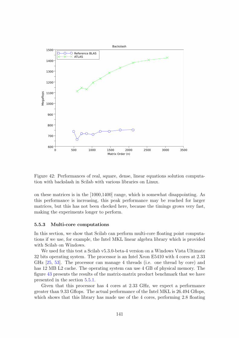
Reference BLASATLAS

600

700

800

900

1000

1100

1200

1300

1400

1500

0 500 1000 1500 2000 2500 3000 3500

Backslash

Matrix Order (n)

Meg

aflop

s

Figure 42: Performances of real, square, dense, linear equations solution computa-tion with backslash in Scilab with various libraries on Linux.

on these matrices is in the [1000,1400] range, which is somewhat disappointing. Asthis performance is increasing, this peak performance may be reached for largermatrices, but this has not been checked here, because the timings grows very fast,making the experiments longer to perform.

5.5.3 Multi-core computations

In this section, we show that Scilab can perform multi-core floating point computa-tions if we use, for example, the Intel MKL linear algebra library which is providedwith Scilab on Windows.

We used for this test a Scilab v5.3.0-beta-4 version on a Windows Vista Ultimate32 bits operating system. The processor is an Intel Xeon E5410 with 4 cores at 2.33GHz [25, 53]. The processor can manage 4 threads (i.e. one thread by core) andhas 12 MB L2 cache. The operating system can use 4 GB of physical memory. Thefigure 43 presents the results of the matrix-matrix product benchmark that we havepresented in the section 5.5.1.

Given that this processor has 4 cores at 2.33 GHz, we expect a performancegreater than 9.33 Gflops. The actual performance of the Intel MKL is 26.494 Gflops,which shows that this library has made use of the 4 cores, performing 2.8 floating

141

Library N User Time (s) MflopsIntel MKL 4766 8.172 26494ATLAS 1595 3.698 2194Ref. BLAS 444 0.125 1400

Figure 43: The performance of the matrix-matrix product on a 4 cores system onWindows with various libraries.

point operations by cycle. On the other side, the ATLAS and Ref-BLAS librariesdo not use the 4 cores of this machine and get much lower results.


In the section 5.2.3, we analyzed the performances of a summation algorithm. Itcould be pointed that the accuracy of a sum may depend on the size of the data andon the particular values in the dataset. This is analyzed, for example, by Wilkinson[54] and Higham [23]. More precisely, it can be shown that a dataset can be ill-conditionned with respect to the sum, for example if the values are of mixed signs(that is, some are positive while some others are negative), and of very differentmagnitude. In this case, we may observe that the relative error of the sum may belarge.

In this document, we have focused mainly on performance and refer to the pre-vious references for the accuracy issues. In practice, it is difficult to completelyseparate the two topics. Indeed, it is more easy to get better performances if wecompletely neglect the accuracy issues. This is why it is safe to consider optimiza-tions only after we have a sufficiently large basis of tests, including both correctnessand accuracy. This ensures that, during the ”optimization” process, we do notintroduce a bug or, worse, an unnecessary error in the result.

A topic which is closely associated with vectorization of Scilab algorithms ismatrix indexing, that is, selecting a subset of elements within a matrix. The articleby Eddins and Shure [18] focuses on this topic within the context of Matlab R©, wherethe authors presents indexing of vectors, indexing of matrices with two subscripts,linear indexing and logical indexing based on boolean expressions. Matlab is aregistered trademark of The MathWorks.

In the section 5.2.1, we have presented several methods associated with compilingprinciples. The ”Dragon Book” [5] is a classical reference on the subject of compilers.The book provides a thorough introduction to compiler design, including lexicalanalysis, regular expressions, finite state machines and parsing methods.

In the section 5.4.1, we briefly presented the ATLAS project. Whaley and Don-garra [51] describe an approach for the automatic generation and optimization ofnumerical software for processors with deep memory hierarchies and pipelined func-tional units.

In the section 5.1.3, we presented a Gaussian elimination algorithm and statedthat this algorithm (but not the particular implementation that we presented) isused in Scilab, behind the backslash operator. The actual behavior of the backslashoperator in Scilab is the following. First, we perform a call to the DGETRF LAPACK

142

routine, which decomposes the matrix A into PA = LU , where P is a permutationmatrix, L is a lower triangular matrix and U is an upper triangular matrix. Thediagonal entries of L are unity. Then we call the DGECON LAPACK routine, whichapproximates the inverse of the 1-norm condition number of the matrix A. At thispoint, there are two cases. If the condition number of the matrix is not too large,then the system of linear equations is not ill-conditionned (this is not exact, becausethe condition is only approximated, but the algorithm makes the hypothesis thatthe estimation can be trusted). In this case, we call the DGETRS LAPACK routine,which solves the linear system of equations by using the PA = LU decomposition.More precisely, this step uses row permutations, and then the forward and backwardsubstitutions in order to compute the solution x depending on the right-hand side b.In the other case, that is, if the matrix is ill-conditionned, we use a modified versionof the DGELSY LAPACK routine, which solves the associated least-squares problem.This choice may reduce the accuracy for matrices of intermediate condition [10].

In [39], Cleve Moler analyze the performances of Matlab in various situations,including the computation of the solution of a linear system of equations with thebackslash operator. To measure the performance of the computation, he counts thenumber of flops, by measuring the elapsed time in second with Matlab’s tic and toc

functions, and estimating the number of floating point operations for this particularcomputation. The author uses a random matrix with entries computed from thenormal distribution function and uses the randn function in Matlab. By increasingthe size of the matrix, he observes a peak in the performance, which corresponds tothe size of the cache of the SPARC-10 computer he uses for this test. This machinehas a one megabyte cache, which corresponds to a square matrix of order

-->floor(sqrt (1.e6/8))

ans =

353.

More precisely, Moler uses the definition that associates one megabytes to 220 bytes,but the result is roughly the same. The peak megaflop rate is obtained for a matrixthat just fits in the cache. He states that this cache effect is a consequence of theLINPACK library. He emphasize that this is one of the primary motivations forthe LAPACK project. This paper was written in 1994: Matlab uses the LAPACKlibrary since 2000 [40]. In [16], Jack Dongarra collects various performances on thisbenchmark. Related resources are available on netlib [42].

General resources related to performance improvement for Matlab are availablein [38].

In the section 5.4.3, we have discussed the installation of Scilab on Windows.This topic is discussed further in [14], where Allan Cornet, who is a developerfrom the Scilab Consortium, presents the full installation process of Scilab 5.2.0 onWindows.

In the section 5.4.4, we have presented the installation of a binary version ofATLAS for Scilab on Linux/Ubuntu. Since ATLAS is optimized at build time,it is better to compile ourselve ATLAS on the machine where we plan to use it.This guarantees that the binary that we use is really optimized with respect to theparameters of the current machine (for example, the size of the cache). In [48],Sylvestre Ledru, who is a developper from the Scilab Consortium and maintains the

143

Debian Science package, provides informations about the installation of ATLAS onDebian. This topic is presented in more depth in [30].

There are other references which may help Scilab users on Linux. In [31], Ledrudescribes the installation process for Scilab 5.1.1 on Linux. In [32], Ledru discussesthe update of the management of BLAS and LAPACK packages under Debian. In[29], Ledru presents a method which allows to switch between different optimizedlinear algebra libraries.

In the section 5.1.4, we presented the benchfun function, which measures theperformances of a given function. Alternatively, we can use the Scibench module[6], which is provided on ATOMS. The goal of the Scibench project is to providetools to measure the performances of a function. Moreover, the module provides acollection of benchmark scripts to measure the performance of Scilab. Within theScibench module, the scibench benchfun function has the same goal as benchfun,which has been presented in the section 5.1.4.

5.7 Exercises

Exercise 5.1 (Gauss pivoting) In the section 5.1.3, we have presented two func-tions gausspivotalnaive and gausspivotal which both implement the Gaussianelimination algorithm with row pivoting. Use the benchfun function and comparethe actual performances of these two functions.

Exercise 5.2 (Combinations) Consider two 1-by-n matrices of doubles x andy. We would like to create a function generating at 2-by-m matrix c containing allthe combinations of the vectors x and y, with m = n2. That is, we would like toproduce the couples [x(1);y(1)], [x(1);y(2)], [x(1);y(3)], ..., [x(n);y(n)].For example, consider the following matrices x and y.

-->x = [10 11 12];

-->y = [13 14 15];

We would like to generate the following matrix c:

-->c

c =

10. 10. 10. 11. 11. 11. 12. 12. 12.

13. 14. 15. 13. 14. 15. 13. 14. 15.

• Create a naive implementation to produce the matrix c.

• Use the Kronecker product .*. and create a vectorized function to producethe matrix c.

• Use matrix extractions to create a vectorized function to produce the matrixc.

6 Acknowledgments

I would like to thank Allan Cornet, Sylvestre Ledru, Bruno Jofret and BernardHugueney for the help they provided during the preparation of this document. I

144

thank Sylvestre Ledru for the informations he shared with respect to the packaging ofATLAS on Debian. Bruno Jofret introduced me to the management of the memoryin the stack of Scilab. I thank Allan Cornet for the informations he shared withrespect to the packaging of ATLAS and the Intel MKL on Windows. I thank BenoitGoepfert and Stanislav V. Kroter for there comments on this document. I thankSerge Steer and Mike Pages for their discussions on hypermatrices.

145

7 Answers to exercises

7.1 Answers for section 2

Answer of Exercise 2.1 (Maximum stack size) The result of the algorithm which sets the sizeof the stack depends on the operating system. This is the result on a Windows machine :

-->format (25)

-->stacksize("max")

-->stacksize ()

ans =

110054096. 34881.

and this is the result on a Linux machine

-->format (25)

-->stacksize("max")

-->stacksize ()

ans =

28176384. 35077.

Answer of Exercise 2.2 (who user ) The following session is the result on a Linux machine.

-->who_user ()

User variables are:

home

Using 7 elements out of 4990798

-->A=ones (100 ,100);

-->who_user ()

User variables are:

A home

Using 10009 elements out of 4990796

-->home

home =

/home/mb

Actually, there may be other user-defined variable which may be displayed by the who user

function. For example, I have installed the ATOMS ”uncprb” module, and here is what I get atstartup.

-->who_user ()

User variables are:

uncprblib

Using 217 elements ouf of 4990785

This is because the uncprblib variable contains the library associated with this particular module.

Answer of Exercise 2.3 (whos ) The following session presents the output of the whos

function, which displays the name, type, size and bytes required by all the variables in the currentenvironment.

-->whos

Name Type Size Bytes

$ polynomial 1 by 1 56

%driverName string* 1 by 1 40

%e constant 1 by 1 24

%eps constant 1 by 1 24

[...]

146

guilib library 488

helptoolslib library 728

home string 1 by 1 56

integerlib library 1416

interpolationlib library 336

[...]


Answer of Exercise 3.1 (Searching for files) The following function searchSciFilesInDir

searches for these files in the given directory.

function filematrix=searchSciFilesInDir(directory ,funname)

filematrix = []

lsmatrix = ls ( directory )’;

for f = lsmatrix

issci = regexp(f,"/(.*). sci/");

if ( issci <> [] ) then

scifile = fullfile ( directory , f )

funname ( scifile )

filematrix($+1) = scifile

end

end

endfunction

In our example, we will simply display the file name. The following function mydisplay uses themprintf function to display the file name into the console. In order to print a brief message, weskip the directory name from the displayed string. In order to separate the name of the directoryfrom the name of the file, we use the fileparts function.

function mydisplay ( filename )

[path ,fname ,extension ]= fileparts(filename)

mprintf ("%s%s\n",fname ,extension)

endfunction

In the following session, we use the searchSciFilesInDir function to print the scilab scriptsfrom the Scilab directory containing the macros associated with polynomials. The SCI variablecontains the name of the directory containing the Scilab directory. In order to compute the absolutefilename of the directory containing the macros, we use the fullfile function, which gathers itsinput arguments into a single string, separating directories with the separator corresponding to thecurrent operating system (i.e. the slash ”/” under Linux and the backslash ”\” under Windows).

-->directory = fullfile(SCI ,"modules","polynomials","macros")

directory =

/home/username/scilab -5.2.2/ share/scilab/modules/

polynomials/macros

-->filematrix = searchSciFiles ( directory , mydisplay );

invr.sci

polfact.sci

cmndred.sci

[...]

horner.sci

rowcompr.sci

htrianr.sci

147

Answer of Exercise 3.2 (Querying typed lists) We have already seen that the definedfieldsfunction returns the floating point integers associated with the locations of the fields in the datastructure. This is not exactly what we need here, but it is easy to build our own function over thisbuilding block. The following isfielddef function takes a typed list tl and a string fieldname

as input arguments and returns a boolean bool which is true if the field is defined and false if not.First, we compute ifield, which is the index of the field fieldname. To do this, we search thestring fieldname in the complete list of fields defined in tl(1) and use find to find the requiredindex. Then, we use the definedfields function to get the matrix of defined indices df. Then wesearch the index ifield in the matrix df. If the search succeeds, then the variable k is not empty,which means that the field is defined. If the search fails, then the variable k is empty, which meansthat the field is not defined.

function bool = isfielddef ( tl , fieldname )

ifield = find(tl(1)== fieldname)

df = definedfields ( tl )

k = find(df== ifield)

bool = ( k <> [] )

endfunction

Although the program is rather abstract, it remains simple and efficient. Its main virtue is toshow how typed lists can lead to very dynamic data structures.


Answer of Exercise 5.1 (Gauss pivoting) We use the following script, which creates a 100-by-100 matrix of doubles and use it to compare the performances of gausspivotalnaive andgausspivotal.

stacksize("max");

n = 100;

A = grand(n,n,"def");

e = ones(n,1);

b = A * e;

benchfun("naive",gausspivotalnaive ,list(A,b),1,10);

benchfun("fast",gausspivotal ,list(A,b),1,10);


naive: 10 iterations , mean =1.541300 , min =1.482000 , max =2.03

fast: 10 iterations , mean =0.027000 , min =0.010000 , max =0.070000

In this case, for this matrix size, the average performance improvement is 1.5413/0.027=57.08.In fact, it could be larger, provided that we use sufficiently large matrices. For n=200, we haveobserved a performance ratio larger than 100.

Answer of Exercise 5.2 (Combinations) We consider two vectors x and y, with n entries.The goal of this exercise is to create a function able to generate a 2-by-m matrix c containing allthe combinations of the vectors x and y, where m = n2.

Our first idea is to use two nested loops: this idea is implemented in the following function.The first loop on ix enumerates the entries in x, while the second loop on iy enumerates the entriesin y. The algorithm is initialized with k=1. Each time we create a new combination, we store it inthe kth column of c, and then we increase k.

function c = combinatevectorsSlow ( x , y )

cx=size(x,"c")

cy=size(y,"c")

c=zeros(2,cx*cy)

k = 1

for ix = 1 : cx

148

for iy = 1 : cy

c(1:2,k) = [x(ix);y(iy)]

k = k + 1

end

end

endfunction

The previous function works, but is slow because it requires to perform n2 loops. Therefore,the goal is to remove these two nested loops and to generate the combinations with vectorizedstatements.

Our second idea is to use the Kronecker product to generate all the combinations in just onestatement. The following session shows the basic idea to generate all the combinations of thevectors [10 11 12] and [13 14 15].

-->[10 11 12] .*. [1 1 1]

ans =

10. 10. 10. 11. 11. 11. 12. 12. 12.

-->[1 1 1] .*. [13 14 15]

ans =

13. 14. 15. 13. 14. 15. 13. 14. 15.

The following implementation is a direct generalization of the previous session.

function c = combinatevectorsKron ( x , y )

cx=size(x,"c")

cy=size(y,"c")

c(1,:) = x .*. ones(1,cy)

c(2,:) = ones(1,cx) .*. y

endfunction

Our third idea is to use the matrix extraction operations. Indeed, the first row in c is justthe copy of the vector x, three times. This is why we create a matrix of repeated indices, basedon matrix extraction. The repeated indices are also created with repeated indices with matrixextraction. These ideas are presented in the following session, which computes the first row inc. In this session, we first create the indices i1 from 1 to 3. Then we create the indices j1 byrepeatedly extracting the row i1. Then we create k1 by using the matrix function, which convertsthe j1 matrix into a row vector of indices. Finally, we use k1 as indices of the columns in x.

-->x = [10 11 12];

-->i1 = 1:3

i1 =

1. 2. 3.

-->j1 = i1 ([1;1;1] ,:)

j1 =

1. 2. 3.

1. 2. 3.

1. 2. 3.

-->k1 = matrix(j1 ,1,9)

j1 =

1. 1. 1. 2. 2. 2. 3. 3. 3.

-->x(:,k1)

ans =

10. 10. 10. 11. 11. 11. 12. 12. 12.

We can use the same principles to generate the second row in c. But the entries are not justrepeated, they are also alternated. In order to do this, we use the same idea as previously, buttranspose the indices before we convert the matrix of indices into a vector of indices.

-->y = [13 14 15];

-->i2 = 1:3

149

i2 =

1. 2. 3.

-->j2 = i2 ([1;1;1] ,:)

j2 =

1. 2. 3.

1. 2. 3.

1. 2. 3.

-->k2 = matrix(j2 ’,1,9)

k2 =

1. 2. 3. 1. 2. 3. 1. 2. 3.

-->y(:,k2)

ans =

13. 14. 15. 13. 14. 15. 13. 14. 15.

In the previous session, it is important to notice the single quote operator in the expressionmatrix(j2’,1,9). The following script is a direct generalization of the previous ideas.

function c = combinatevectorsExtr ( x , y )

// Returns all combinations of the two row vectors x and y

cx=size(x,"c")

cy=size(y,"c")

//

i1 = 1:cx

j1 = i1(ones(cy ,1) ,:)

k1 = matrix(j1 ,1,cx*cy)

//

i2 = 1:cy

j2 = i2(ones(cx ,1) ,:)

k2 = matrix(j2 ’,1,cx*cy)

//

c(1,:)=x(:,k1)

c(2,:)=y(:,k2)

endfunction

In the following session, we use the benchfun function to compare the performances of theprevious functions.

n = 300;

x=(1:n);

y=(1:n);

benchfun("Slow",combinatevectorsSlow ,list(x,y),1,10);

benchfun("Kron.",combinatevectorsKron ,list(x,y),1,10);

benchfun("Extr.",combinatevectorsExtr ,list(x,y),1,10);

The previous script typically produces the following output.

Slow: 10 iterations , mean =0.24010 , min =0.23700 , max =0.25000

Kron.: 10 iterations , mean =0.01440 , min =0.01300 , max =0.02200

Extr.: 10 iterations , mean =0.00960 , min =0.00700 , max =0.01500

We see that the implementation based on the Kronecker product is more than 10 times faster on theaverage. We notice that there is no significant difference between the combinatevectorsKron andcombinatevectorsExtr functions, although combinatevectorsExtr seems a little faster. Thismay be explained by the fact that combinatevectorsKron performs many floating point multipli-cations, which are unnecessary since one of the operands is unity.

150

References

[1] ATLAS – Automatically Tuned Linear Algebra Software. http://math-atlas.sourceforge.net.

[2] Blas – Basic Linear Algebra Subprograms. http://www.netlib.org/blas.

[3] Lapack – Linear Algebra PACKage. http://www.netlib.org/lapack.

[4] The Linpack benchmark. http://www.top500.org/project/linpack.

[5] Alfred V. Aho, Ravi Sethi, and Jeffrey D. Ullman. Compilers: principles,techniques, and tools. Addison-Wesley Longman Publishing Co., Inc., Boston,MA, USA, 1986.

[6] Michael Baudin. Scibench. http://atoms.scilab.org/toolboxes/scibench.

[7] Michael Baudin. How to emulate object oriented programming in Scilab. http://wiki.scilab.org/Emulate_Object_Oriented_in_Scilab, 2008.

[8] Michael Baudin. Apifun - Check input arguments in macros. http://forge.

scilab.org/index.php/p/apifun/, 2010.

[9] Michael Baudin. The derivative function does not protect against conflictsbetween user-defined functions and developper-defined variables. http://

bugzilla.scilab.org/show_bug.cgi?id=7104, 2010.

[10] Michael Baudin. The help page of backslash does not print the singularity level- bug report #7497. http://bugzilla.scilab.org/show_bug.cgi?id=7497,July 2010.

[11] Michael Baudin. The integrate function does not protect against conflictsbetween user-defined functions and developper-defined variables. http://

bugzilla.scilab.org/show_bug.cgi?id=7103, 2010.

[12] Michael Baudin. The neldermead component does not protect under partic-ular user-defined objective functions. http://bugzilla.scilab.org/show_

bug.cgi?id=7102, 2010.

[13] Michael Baudin. There is no pascal function - bug report #7670. http://

bugzilla.scilab.org/show_bug.cgi?id=7670, August 2010.

[14] Allan Cornet. Scilab installation on Windows. http://wiki.scilab.org/

howto/install/windows, 2009.

[15] J. J. Dongarra, Jermey Du Cruz, Sven Hammerling, and I. S. Duff. Algorithm679: A set of level 3 basic linear algebra subprograms: model implementationand test programs. ACM Trans. Math. Softw., 16(1):18–28, 1990.

[16] Jack J. Dongarra. Performance of various computers using standard linear equa-tions software. http://www.netlib.org/benchmark/performance.ps, 2013.

151





http://www.top500.org/project/linpack

http://atoms.scilab.org/toolboxes/scibench

http://wiki.scilab.org/Emulate_Object_Oriented_in_Scilab


http://forge.scilab.org/index.php/p/apifun/

http://forge.scilab.org/index.php/p/apifun/

http://bugzilla.scilab.org/show_bug.cgi?id=7104









http://wiki.scilab.org/howto/install/windows

http://wiki.scilab.org/howto/install/windows

http://www.netlib.org/benchmark/performance.ps

[17] William H. Duquette. Snit’s not incr tcl. http://www.wjduquette.com/snit/.

[18] Steve Eddins and Loren Shure. Matrix indexing in Matlab. http://www.

mathworks.com.

[19] Jean-Luc Fontaine. Stooop. http://jfontain.free.fr/stooop.html.

[20] Jeffrey Friedl. Mastering Regular Expressions. O’Reilly Media, Inc., 2006.

[21] Gene H. Golub and Charles F. Van Loan. Matrix computations (3rd ed.). JohnsHopkins University Press, Baltimore, MD, USA, 1996.

[22] Philip Hazel. Pcre – Perl Compatible Regular Expressions. http://www.pcre.org/.

[23] Nicholas J. Higham. Accuracy and Stability of Numerical Algorithms. Soci-ety for Industrial and Applied Mathematics, Philadelphia, PA, USA, secondedition, 2002.

[24] Intel. Intel Math Kernel Library. http://software.intel.com/en-us/

intel-mkl/.

[25] Intel. Intel Xeon Processor E5410. http://ark.intel.com/Product.aspx?

id=33080, 2010.

[26] D. E. Knuth. The Art of Computer Programming, Volume 2, SeminumericalAlgorithms. Third Edition, Addison Wesley, Reading, MA, 1998.

[27] Donald E. Knuth. Fundamental Algorithms, volume 1 of The Art of ComputerProgramming. Addison-Wesley, Reading, Massachusetts, second edition, 1973.

[28] Sylvestre Ledru. Localization. http://wiki.scilab.org/Localization.

[29] Sylvestre Ledru. Handle different versions of BLAS and LAPACK. http:

//wiki.debian.org/DebianScience/LinearAlgebraLibraries, 2010.

[30] Sylvestre Ledru. Linear algebra libraries in Debian. http://people.debian.

org/~sylvestre/presentation-linear-algebra.pdf, August 2010.

[31] Sylvestre Ledru. Scilab installation under linux. http://wiki.scilab.org/

howto/install/linux, 2010.

[32] Sylvestre Ledru. Update of the linear algebra libraries in Debian. http://

sylvestre.ledru.info/blog, April 2010.

[33] Pierre Marechal. Code conventions for the Scilab programming language. http://wiki.scilab.org, 2010.

[34] The Mathworks. Matlab - Product Support - 1106 - Memory ManagementGuide. http://www.mathworks.com/support/tech-notes/1100/1106.html.

[35] The Mathworks. Matlab - Product Support - 1107 - Avoiding Out of MemoryErrors. http://www.mathworks.com/support/tech-notes/1100/1107.html.

152

http://www.wjduquette.com/snit/

http://www.mathworks.com


http://jfontain.free.fr/stooop.html

http://www.pcre.org/

http://www.pcre.org/

http://software.intel.com/en-us/intel-mkl/

http://software.intel.com/en-us/intel-mkl/

http://ark.intel.com/Product.aspx?id=33080

http://ark.intel.com/Product.aspx?id=33080

http://wiki.scilab.org/Localization

http://wiki.debian.org/DebianScience/LinearAlgebraLibraries

http://wiki.debian.org/DebianScience/LinearAlgebraLibraries

http://people.debian.org/~sylvestre/presentation-linear-algebra.pdf

http://people.debian.org/~sylvestre/presentation-linear-algebra.pdf

http://wiki.scilab.org/howto/install/linux

http://wiki.scilab.org/howto/install/linux

http://sylvestre.ledru.info/blog

http://sylvestre.ledru.info/blog

http://wiki.scilab.org


http://www.mathworks.com/support/tech-notes/1100/1106.html


[36] The Mathworks. Matlab - Product Support - 1110 - Maximum Matrix Sizeby Platform. http://www.mathworks.com/support/tech-notes/1100/1110.html.

[37] The Mathworks. Matlab - Technical Solution - What are the benefits of 64-bit Matlab versus 32-bit Matlab? http://www.mathworks.com/support/

solutions/en/data/1-YVO5H/index.html.

[38] The Mathworks. Techniques for improving performance. http://www.

mathworks.com/help/techdoc/matlab_prog/f8-784135.html.

[39] Cleve Moler. Benchmarks: Linpack and Matlab - Fame and fortune frommegaflops. http://www.mathworks.com/company/newsletters/news_notes/pdf/sumfall94cleve.pdf, 1994.

[40] Cleve Moler. Matlab incorporates LAPACK. http://www.mathworks.com,2000.

[41] Cleve Moler. The origins of Matlab, December 2004. http://www.mathworks.fr.

[42] netlib.org. Benchmark programs and reports. http://www.netlib.org/

benchmark/.

[43] Mathieu Philippe, Djalel Abdemouche, Fabrice Leray, Jean-Baptiste Silvy, andPierre Lando. modules/graphics/includes/ObjectStructure.h. http://gitweb.scilab.org.

[44] Bruno Pincon. Quelques tests de rapidite entre differents logiciels matriciels.http://wiki.scilab.org/Emulate_Object_Oriented_in_Scilab, 2008.

[45] pqnelson. Object oriented C. http://pqnelson.blogspot.com/2007/09/

object-oriented-c.html.

[46] W. H. Press, Saul A. Teukolsky, William T. Vetterling, and Brian P. Flannery.Numerical Recipes in C, Second Edition. Cambridge University Press, 1992.

[47] Axel-Tobias Schreiner. Object-oriented programming with ANSI C. www.cs.

rit.edu/~ats/books/ooc.pdf.

[48] Debian Science. README.Debian. http://anonscm.debian.org/viewvc/

debian-science/packages/atlas/trunk/debian, 2010.

[49] Enrico Segre. Scilab function variables: representation, manipulation. http:

//wiki.scilab.org, 2007.

[50] Enrico Segre. Scoping of variables in Scilab. http://wiki.scilab.org/howto/global_and_local_variables, 2007.

153



http://www.mathworks.com/support/solutions/en/data/1-YVO5H/index.html

http://www.mathworks.com/support/solutions/en/data/1-YVO5H/index.html

http://www.mathworks.com/help/techdoc/matlab_prog/f8-784135.html

http://www.mathworks.com/help/techdoc/matlab_prog/f8-784135.html

http://www.mathworks.com/company/newsletters/news_notes/pdf/sumfall94cleve.pdf

http://www.mathworks.com/company/newsletters/news_notes/pdf/sumfall94cleve.pdf


http://www.mathworks.fr

http://www.mathworks.fr

http://www.netlib.org/benchmark/

http://www.netlib.org/benchmark/

http://gitweb.scilab.org

http://gitweb.scilab.org


http://pqnelson.blogspot.com/2007/09/object-oriented-c.html

http://pqnelson.blogspot.com/2007/09/object-oriented-c.html

www.cs.rit.edu/~ats/books/ooc.pdf

www.cs.rit.edu/~ats/books/ooc.pdf

http://anonscm.debian.org/viewvc/debian-science/packages/atlas/trunk/debian

http://anonscm.debian.org/viewvc/debian-science/packages/atlas/trunk/debian



http://wiki.scilab.org/howto/global_and_local_variables

http://wiki.scilab.org/howto/global_and_local_variables

[51] R. Clint Whaley and Jack J. Dongarra. Automatically tuned linear algebrasoftware. In Supercomputing ’98: Proceedings of the 1998 ACM/IEEE confer-ence on Supercomputing (CDROM), pages 1–27, Washington, DC, USA, 1998.IEEE Computer Society.

[52] R. Clint Whaley, Antoine Petitet, R. Clint, Whaley Antoine, Petitet Jack,and Jack J. Dongarra. Automated empirical optimizations of software and theATLAS project, 2000.

[53] Wikipedia. Intel Xeon — Wikipedia, the free encyclopedia. http://en.

wikipedia.org/wiki/Xeon, 2010.

[54] James Hardy Wilkinson. Rounding errors in algebraic processes. Prentice Hall,1963.

154

http://en.wikipedia.org/wiki/Xeon

http://en.wikipedia.org/wiki/Xeon

Index

[], 67add param, 76argn, 60check param, 82clear, 15deff, 54det, 25error, 71fullfile, 12get function path, 54get param, 76getos, 12gettext, 71horner, 24init param, 76list, 30poly, 22regexp, 22roots, 24stacksize, 6string, 18tic, 103timer, 103tlist, 33toc, 103typeof, 16, 54type, 16, 54varargin, 60varargout, 60warning, 71who, 11MSDOS, 12SCIHOME, 12SCI, 12TMPDIR, 12

ATLAS, 130

BLAS, 129

callback, 57, 58

DGEMM, 130

flops, 137

funcprot, 56, 57

Intel, 130interpreter, 115

LAPACK, 130

macros, 54MKL, 130

PCRE, 18polynomials, 22primitive, 54profile function, 106

regular expression, 18

vectorization, 103

155

Programming in Scilab - SPACE · Programming in Scilab Micha el Baudin September 2011 Abstract In...

Documents

Transcript of Programming in Scilab - SPACE · Programming in Scilab Micha el Baudin September 2011 Abstract In...