Programming in Scilabforge.scilab.org/index.php/p/docprogscilab/source/tree/2/en_US/... ·...

Programming in Scilab

Michael Baudin

May 2009

Abstract

In this chapter, we present programming in Scilab. As programming is anassociation between data structures and algorithms, the first part is dedicatedto data structures, while the second part focuses on functions.

In the first part, we present the integer and string data types in more depth.We also present how we can manage the memory of Scilab. An analysis of listsand typed lists is presented. We present a method which allows to emulateobject-oriented programming, based on a particular use of typed lists. Wefinally present how to overload basic operations on typed lists.

In the second part, we show how to design flexible functions. We presentthe use of callbacks, which allow to let the user of a function customize a partof an algorithm. Then we present functions which allow to protect againstwrong uses of a function. We analyze methods to design functions with avariable number of input or output arguments, and show common ways toprovide default values. We show a simple method to overcome the problemcaused by positional input arguments. We present the parameters module,which allows to solve the problem of designing a function with a large numberof parameters.

In the last section, we present methods which allows to achieve good per-formances. We emphasize the use of vectorized functions, which allow toget the most of Scilab performances, via calls to highly optimized libraries.We present to extend Scilab’s capabilities, by installing modules manually orfrom the ATOMS packaging system. We present the creation of interfaces toexternal softwares, provided either as an executable or as a C source code.

Contents

1 Variable and memory management 31.1 Management of the stack : stacksize . . . . . . . . . . . . . . . . . 31.2 More on memory management . . . . . . . . . . . . . . . . . . . . . . 41.3 The list of variables and the function who . . . . . . . . . . . . . . . . 51.4 Portability variables and functions . . . . . . . . . . . . . . . . . . . . 61.5 Destroying variables : clear . . . . . . . . . . . . . . . . . . . . . . . 81.6 The type and typeof functions . . . . . . . . . . . . . . . . . . . . . 9

1

2 Special data types 92.1 Strings . . . . . . . . . . . . . . . . . . . . . . . . . . . . . . . . . . . 92.2 Conversions of integers . . . . . . . . . . . . . . . . . . . . . . . . . . 132.3 Polynomials . . . . . . . . . . . . . . . . . . . . . . . . . . . . . . . . 132.4 Hypermatrices . . . . . . . . . . . . . . . . . . . . . . . . . . . . . . . 162.5 Lists . . . . . . . . . . . . . . . . . . . . . . . . . . . . . . . . . . . . 172.6 Typed lists . . . . . . . . . . . . . . . . . . . . . . . . . . . . . . . . 202.7 Emulating object oriented with typed lists . . . . . . . . . . . . . . . 24

2.7.1 Limitations of positional arguments . . . . . . . . . . . . . . . 242.7.2 A classical scheme . . . . . . . . . . . . . . . . . . . . . . . . 252.7.3 A ”person” class in Scilab . . . . . . . . . . . . . . . . . . . . 26

2.8 Overloading with typed lists . . . . . . . . . . . . . . . . . . . . . . . 282.9 Exercises . . . . . . . . . . . . . . . . . . . . . . . . . . . . . . . . . . 30

3 Management of functions 313.1 How to inquire about functions . . . . . . . . . . . . . . . . . . . . . 313.2 Functions are not reserved . . . . . . . . . . . . . . . . . . . . . . . . 333.3 Functions are variables . . . . . . . . . . . . . . . . . . . . . . . . . . 333.4 Callbacks . . . . . . . . . . . . . . . . . . . . . . . . . . . . . . . . . 353.5 Protection against wrong uses: warning and error . . . . . . . . . . 353.6 Managing a variable number of arguments . . . . . . . . . . . . . . . 373.7 Optional arguments and default values . . . . . . . . . . . . . . . . . 433.8 Functions with variable type input arguments . . . . . . . . . . . . . 453.9 Using parameters . . . . . . . . . . . . . . . . . . . . . . . . . . . . 46

3.9.1 Overview of the module . . . . . . . . . . . . . . . . . . . . . 473.9.2 A practical case . . . . . . . . . . . . . . . . . . . . . . . . . . 493.9.3 Issues with the parameters module . . . . . . . . . . . . . . . 52

3.10 Issues with callbacks . . . . . . . . . . . . . . . . . . . . . . . . . . . 543.11 Callbacks with additionnal arguments . . . . . . . . . . . . . . . . . . 543.12 Robust functions . . . . . . . . . . . . . . . . . . . . . . . . . . . . . 543.13 Exercises . . . . . . . . . . . . . . . . . . . . . . . . . . . . . . . . . . 54

4 Performances 544.1 Measuring the performance . . . . . . . . . . . . . . . . . . . . . . . 554.2 An example of performance analysis . . . . . . . . . . . . . . . . . . . 564.3 The interpreter . . . . . . . . . . . . . . . . . . . . . . . . . . . . . . 594.4 BLAS, LAPACK, ATLAS and the MKL . . . . . . . . . . . . . . . . 614.5 Profiling a function . . . . . . . . . . . . . . . . . . . . . . . . . . . . 624.6 The danger of dymanic matrices . . . . . . . . . . . . . . . . . . . . . 694.7 References and notes . . . . . . . . . . . . . . . . . . . . . . . . . . . 69

5 Answers to exercises 715.1 Answers for section 1 . . . . . . . . . . . . . . . . . . . . . . . . . . . 71

Bibliography 73

Index 74

2

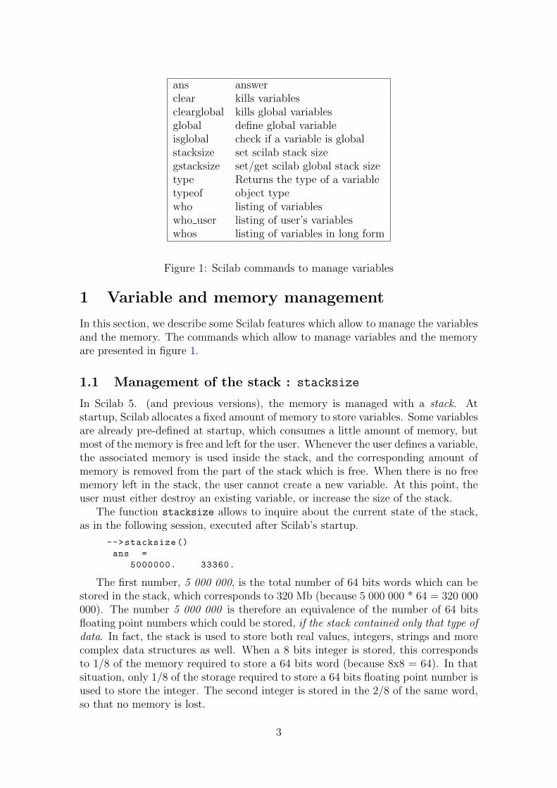
ans answerclear kills variablesclearglobal kills global variablesglobal define global variableisglobal check if a variable is globalstacksize set scilab stack sizegstacksize set/get scilab global stack sizetype Returns the type of a variabletypeof object typewho listing of variableswho user listing of user’s variableswhos listing of variables in long form

Figure 1: Scilab commands to manage variables

1 Variable and memory management

In this section, we describe some Scilab features which allow to manage the variablesand the memory. The commands which allow to manage variables and the memoryare presented in figure 1.

1.1 Management of the stack : stacksize

In Scilab 5. (and previous versions), the memory is managed with a stack. Atstartup, Scilab allocates a fixed amount of memory to store variables. Some variablesare already pre-defined at startup, which consumes a little amount of memory, butmost of the memory is free and left for the user. Whenever the user defines a variable,the associated memory is used inside the stack, and the corresponding amount ofmemory is removed from the part of the stack which is free. When there is no freememory left in the stack, the user cannot create a new variable. At this point, theuser must either destroy an existing variable, or increase the size of the stack.

The function stacksize allows to inquire about the current state of the stack,as in the following session, executed after Scilab’s startup.

-->stacksize ()

ans =

5000000. 33360.

The first number, 5 000 000, is the total number of 64 bits words which can bestored in the stack, which corresponds to 320 Mb (because 5 000 000 * 64 = 320 000000). The number 5 000 000 is therefore an equivalence of the number of 64 bitsfloating point numbers which could be stored, if the stack contained only that type ofdata. In fact, the stack is used to store both real values, integers, strings and morecomplex data structures as well. When a 8 bits integer is stored, this correspondsto 1/8 of the memory required to store a 64 bits word (because 8x8 = 64). In thatsituation, only 1/8 of the storage required to store a 64 bits floating point number isused to store the integer. The second integer is stored in the 2/8 of the same word,so that no memory is lost.

3

The second number, i.e 33 360, is the number of 64 bits words which are alreadyused.

That means that only 5 000 000 - 33 360 = 4966640 units of 64 bits words arefree for the user. Because

√5000000 ≈ 2236, that means that, with these settings, it

is not possible to create a dense matrix with more than 2236× 2236 elements. Thisis probably sufficient in most cases, but might be a limitation for some applications.

In the following Scilab session, we show that creating a random 2300 × 2300dense matrix generates an error, while creating a 2200× 2200 matrix is possible.

-->A=rand (2300 ,2300)

!--error 17

rand: stack size exceeded (Use stacksize function to increase it).

-->clear A

-->A=rand (2200 ,2200);

The stacksize("max") function allows to configure the size of the stack so thatit allocates the maximum possible amount of memory on the system. The followingscript gives an example of this function, as executed on a Linux laptop with 1 Gbmemory. The format function is used so that all the digits are displayed.

-->format (25)

-->stacksize("max")

-->stacksize ()

ans =

28176384. 35077.

We can see that, this time, the total memory available in the stack correspondsto 28 176 384 units of 64 bits words, which corresponds to 1.8 Gb (because 28 176384 * 64 = 1 803 288 576). The maximum dense matrix which can be stored is now5308× 5308 (because

√(28176384) ≈ 5308).

The user might still be able to manage sparse matrices with much larger di-mensions than the dense matrices previously used, but, in any case, the total usedmemory can exceed the size of the stack.

The algorithm used by the stacksize("max") function is the following. Themaximum possible amount of memory which can be allocated is computed. If thatamount of memory is lower than the current one, the current one is kept. If not, thismaximum memory is allocated, the current state is copied from the current memoryinto the new memory, and the old memory is unallocated.

1.2 More on memory management

On 32 bits systems, the memory is adressed with 32 bits integers. Therefore, itwould seem that the maximum available memory in Scilab would be 232 ≈ 4.2 Gb.In fact the maximum available memory depends on the operating system in thefollowing way.

On Windows 32 bits systems, only 2 Gb of memory are available in practice.This is because 2 Gb are reserved for the system. Some 32 bits unix systems alsoreserve 2 Gb of memory for the system. This is why in practice, only 2 Gb can beused by Scilab on most 32 bits systems.

On 64 bits systems, the memory is adressed by the operating system with 64 bitsintegers. Therefore, it would seem that the maximum available memory in Scilab

4

would be 264 ≈ 1.8 × 1010 Gb. First, this is larger than any available physicalmemory on the market (in 2009). Second, Scilab’s stack is still managed internallywith 32 bits integers, so that no more memory is usable in practice.

Still, Scilab users may experience that some particular linear algebra or graphicalfeature works on 64 bits systems while it does not work on a 32 bits system in aparticular situation. This is because Scilab uses its stack to store its variables, but,depending on the implementation associated with each particular function, it mayuse either the stack or the memory of the system (by using dynamic allocation) forintermediate results. This is because, for historical reasons, the source code usedinternally in Scilab does not always use the same method to create intermediatearrays. Sometimes, the intermediate variable is created on the stack, and destroyedafterwards. Sometimes, the intermediate variable is allocated in the memory of thesystem and unallocated afterwards.

Some additionnal details about the management of memory in Matlab are givenin [14].

1.3 The list of variables and the function who

The following script shows the behavior of the who function, which shows the currentlist of variables, as well as the state of the stack.

--> who

Your variables are:

whos home matiolib parameterslib

simulated_annealinglib genetic_algorithmslib umfpacklib fft

scicos_pal %scicos_menu %scicos_short %scicos_help

%scicos_display_mode modelica_libs scicos_pal_libs %scicos_lhb_list

%CmenuTypeOneVector %scicos_gif %scicos_contrib scicos_menuslib

scicos_utilslib scicos_autolib spreadsheetlib demo_toolslib

development_toolslib scilab2fortranlib scipadinternalslib scipadlib

soundlib texmacslib with_texmacs tclscilib

m2scilib maple2scilablib metanetgraph_toolslib metaneteditorlib

compatibility_functilib statisticslib timelib stringlib

special_functionslib sparselib signal_processinglib %z

%s polynomialslib overloadinglib optimizationlib

linear_algebralib jvmlib iolib interpolationlib

integerlib dynamic_linklib guilib data_structureslib

cacsdlib graphic_exportlib graphicslib fileiolib

functionslib elementary_functionlib differential_equationlib helptoolslib

corelib PWD %F %T

%nan %inf COMPILER SCI

SCIHOME TMPDIR MSDOS %gui

%pvm %tk %fftw $

%t %f %eps %io

%i %e %pi

using 34485 elements out of 5000000.

and 87 variables out of 9231.

Your global variables are:

%modalWarning demolist %helps %helps_modules

%driverName %exportFileName LANGUAGE %toolboxes

%toolboxes_dir

using 3794 elements out of 10999.

and 9 variables out of 767.

5

SCI the installation directory of the current Scilab installationSCIHOME the directory containing user’s startup filesMSDOS true if the current operating system is WindowsTMPDIR the temporary directory for the current Scilab’s sessionCOMPILER the name of the current compiler[OS,Version]=getos() the name of the current operating system

Figure 2: Portability variables

All the variables which names are ending with ”lib” (as optimizationlib for ex-ample) are associated with Scilab’s internal function libraries. Some variables start-ing with the ”%” character, i.e. %i, %e and %pi, are associated with pre-definedScilab variables because they are mathematical constants. Other variables whichname start with a ”%” character are associated with the precision of floating pointnumbers and the IEEE standard. These variables are %eps, %nan and %inf. Up-case variables SCI, SCIHOME, COMPILER, MSDOS and TMPDIR allow to create portablescripts, i.e. scripts which can be executed independently of the installation directoryor the operating system. These variables are described in the next section.

1.4 Portability variables and functions

There are some pre-defined variables which allow to design portable scripts, thatis, scripts which work equally well on Windows, Linux or Mac. These variablesare presented in table 2. These variables are mainly used when creating externalmodules, but may be of practical value in a large set of situations.

In the following session, we check the values of some pre-defined variables on aLinux machine.

-->SCI

SCI =

/home/myname/Programs/Scilab -5.1/ scilab -5.1/ share/scilab

-->SCIHOME

SCIHOME =

/home/myname /. Scilab/scilab -5.1

-->MSDOS

MSDOS =

F

-->TMPDIR

TMPDIR =

/tmp/SD_8658_

-->COMPILER

COMPILER =

gcc

The TMPDIR variable, which contains the name of the temporary directory, is as-sociated with the current Scilab session: each Scilab session has a unique temporarydirectory. The following is the content of the TMPDIR on my current Linux machine.

-->TMPDIR

TMPDIR =

/tmp/SD_8658_

6

The following is the content of the TMPDIR on my current Windows machine.

-->TMPDIR

TMPDIR =

C:\Users\myname\AppData\Local\Temp\SCI_TMP_4088_

Scilab’s temporary directory is created by Scilab at startup (and is not destroyedwhen Scilab quits). In practice, we may use the TMPDIR in test scripts where we haveto create temporary files. This way, the file system is not polluted with temporaryfiles and there is a little less chance to overwrite important files.

The COMPILER variable is used by scripts which are dynamically compiling andlinking source code into Scilab. We often use the SCIHOME variable to locate the”.startup” file on the current machine.

The MSDOS variable allows to create scripts which manage particular settingsdepending on the operating system. These scripts typically use if statements of thefollowing form.

if ( MSDOS ) then

// Windows statements

else

// Linux statements

end

In practice, consider the situation where we want to call an external programwith the maximum possible portability. Assume that, under Windows, this programis provided by a ”.bat” script while, under Linux, this program is provided by a ”.sh”script. In this situation, we might write a script using the MSDOS variable and theunix function, which executes an external program. Despite its name, the unix

function works equally under Linux and under Windows.

if ( MSDOS ) then

unix("myprogram.bat")

else

unix("myprogram.sh")

end

The previous example shows that it is possible to write a portable Scilab programwhich works in the same way under various operating systems. The situation mightbe even more complicated, because it often happens that the path leading to theprogram is also depending on the operating system. Another situation is when wewant to compile a source code with Scilab, using, for example, the ilib_for_link

or the tbx_build_src functions. In this case, we might want to pass to the com-piler some particular option which depends on the operating system. In all thesesituations, the MSDOS variable allows to make one single source code which executesremains portable across various systems.

If a improved portability is required, the getos function should be used. Thisfunction returns a string containing the name of the current operating system and,optionnaly, its version. In the following session, we call the getos function on aWindows XP machine.

-->[OS,Version ]=getos()

Version =

XP

OS =

7

Windows

The getos function may be typically used in select statements such as the follow-ing.

OS=getos()

select OS

case "Windows" then

disp("Scilab on Windows")

case "Linux" then

disp("Scilab on Linux")

case "Linux" then

disp("Scilab on Solaris")

case "Darwin" then

disp("Scilab on MacOs")

else

error("Scilab on Unknown platform")

end

Notice that the previous script is not really typical, because the main distributionsof Scilab binaries are on Windows, Linux and Mac OS. There is no official binary ofScilab under Solaris.

The SCI variable allows to compute paths relative to the current Scilab instal-lation. The following session shows a sample use of this variable. First, we get thepath of a macro provided by Scilab. Then, we combine the SCI variable with arelative path to the file and pass this to the ls function. Finally, we concatenate theSCI variable with a string containing the relative path to the script and pass it tothe editor function. In both cases, the commands do not depend on the absolutepath to the file, which make them more portable.

-->get_function_path("numdiff")

ans =

/home/myname/Programs/Scilab -5.1/ scilab -5.1/...

share/scilab/modules/optimization/macros/numdiff.sci

-->ls (SCI+"/modules/optimization/macros/numdiff.sci")

ans =

/home/myname/Programs/Scilab -5.1/ scilab -5.1/...

share/scilab/modules/optimization/macros/numdiff.sci

-->editor(SCI+"/modules/optimization/macros/numdiff.sci")

1.5 Destroying variables : clear

Variables can be created at will, when there are needed. They can also be destroyedexplicitly with the clear, when they are not needed anymore. This might be usefulwhen large matrices are to be managed and the memory becomes a problem.

In the following script,we define a large random matrix A. When we try to definea second matrix B, we see that there is no memory left. Therefore, we use the clear

function to destroy the matrix A. Then we are able to create the matrix B.

-->A = rand (2000 ,2000);

-->B = rand (2000 ,2000);

!--error 17

rand: stack size exceeded (Use stacksize function to increase it).

-->clear A

8

-->B = rand (2000 ,2000);

1.6 The type and typeof functions

Scilab can create various types of variables, such as matrices, polynomials, booleans,integers, etc... The type and typeof functions allow to inquire about the particulartype of a given variable. The type function returns a floating point integer whilethe typeof function returns a string.

The table in figure 3 presents the various output values of the type and typeof

functions. In the following session, we create a 2 × 2 matrix and use the type andtypeof to get the type of this matrix.

-->A=eye(2,2)

A =

1. 0.

0. 1.

-->type(A)

ans =

1.

-->typeof(A)

ans =

constant

These two functions are useful when processing the input arguments of a function.This topic will be reviewed later in this document, when we will consider functionmanagement.

When the type of the variable is a tlist or mlist, the value returned by the typeoffunction is the first string in the first list entry

The datatypes cell and struct are special forms of mlists, so that they areassociated with a type equal to 17 and with a typeof equal to ”ce” and ”st”.

2 Special data types

In this section, we analyse Scilab data types which are the most commonly used inpractice. We review strings, integers, polynomials, hypermatrices, lists and typedlists.

2.1 Strings

Although Scilab is not primarily designed as a tool to manage strings, it providesa consistent and powerfull set of functions to manage this data type. A list ofcommands which are associated with Scilab strings is presented in figure 4.

Perhaps the most common string function that we use on a day-to-day basisis the string function. This function allows to convert its input argument into astring. In the following session, we define a row vector and use the string functionto convert it into a string. Then we use the typeof function and check that the str

variable is indeed a string. Finally, we use the size function and check that the str

variable is a 1× 5 matrix of strings.

9

type typeof detail1 ”constant” real or complex constant matrix2 ”polynomial” polynomial matrix4 ”boolean” boolean matrix5 ”sparse” sparse matrix6 ”boolean sparse” sparse boolean matrix7 ”Matlab sparse” Matlab sparse matrix8 ”int8”, ”int16”, ”int32”, matrix of integers stored on 1 2 or 4 bytes

”uint8”, ”uint16” or ”uint32”9 ”handle” matrix of graphic handles10 ”string” matrix of character strings11 ”function” un-compiled function (Scilab code)13 ”function” compiled function (Scilab code)14 ”library unction library15 ”list” list16 ”rational”, ”state-space” or the type typed list (tlist)17 ”hypermat”, ”st”, ”ce” or the type matrix oriented typed list (mlist)128 ”pointer” sparse matrix LU decomposition129 ”size implicit” size implicit polynomial used for indexing130 ”fptr” Scilab intrinsic (C or Fortran code)

Figure 3: The returned values of the type and typeof function

-->x = [1 2 3 4 5];

-->str = string(x)

str =

!1 2 3 4 5 !

-->typeof(str)

ans =

string

-->size(str)

ans =

1. 5.

The string function can take any type of input argument, including matrices, lists,polynomials.

We will see later in this document that a tlist can be used to define a new datatype. In this case, we can define a function which makes to that the string canwork on this new data type in a user-defined way.

We may combine the string and the strcat functions to produce strings whichcan be more easily copied and pasted into scripts or reports. The strcat functionconcatenates its first input argument with the separator defined in the second inputargument. In the following session, we define the row vector x which contains floatingpoint integers. Then we use the strcat function with the blank space separator toproduce a clean string of integers.

-->x = [1 2 3 4 5]

x =

1. 2. 3. 4. 5.

10

string conversion to stringsci2exp converts an expression to a stringstr2code return Scilab integer codes associated with a character stringcode2str returns character string associated with Scilab integer codes

ascii string ascii conversionsblanks create string of blank charactersconvstr case conversionemptystr zero length stringgrep find matches of a string in a vector of stringsjustify justify character arraylength length of objectpart extraction of stringsregexp find a substring that matches the regular expression stringstrcat concatenate character stringsstrchr find the first occurrence of a character in a stringstrcmp compare character stringsstrcmpi compare character strings (case independent)strcspn get span until character in stringstrindex search position of a character string in an other stringstripblanks strips leading and trailing blanks (and tabs) of stringsstrncmp copy characters from stringsstrrchr find the last occurrence of a character in a stringstrrev returns string reversedstrsplit split a string into a vector of stringsstrspn get span of character set in stringstrstr locate substringstrsubst substitute a character string by another in a character stringstrtod convert string to doublestrtok split string into tokenstokenpos returns the tokens positions in a character stringtokens returns the tokens of a character string

Figure 4: Scilab string functions

11

-->strcat(string(x)," ")

ans =

1 2 3 4 5

The previous string can be directly copied and pasted into a source code or a report.It may happen that we design a function which prints datas into the console. Theprevious combination of function is an efficient way of producing compact and factmessages. In the following session, we use the mprintf function to display thecontent of the x variable. We use the %s format, which corresponds to strings. Inorder to produce the string, we combine the strcat and string functions.

-->mprintf("x=[%s]\n",strcat(string(x)," "))

x=[1 2 3 4 5]

The sci2exp function converts an expression into a string. It can be used withthe same purpose as the previous method based on strcat, but the formatting isless flexible. In the following session, we use the sci2exp function to convert a rowmatrix of integers into a 1× 1 matrix of strings.

-->x = [1 2 3 4 5];

-->str = sci2exp(x)

str =

[1,2,3,4,5]

-->size(str)

ans =

1. 1.

Common comparison operators, such as ”<” or ”>” for example, are not definedwhen strings are used. Instead, the strcmp function can be used for that purpose.It returns 1 if the first argument is lexicographically less than the second, or 0 if thetwo strings are equal, or -1 if the second argument is lexicographically less than thefirst. The behaviour of the command is presented in the following session.

-->strcmp("a","b")

ans =

- 1.

-->strcmp("a","a")

ans =

0.

-->strcmp("b","a")

ans =

1.

Given a string, we may want to perform a different processing depending onthe particular nature of the string. The functions presented in the table 5 allow todistinguish between ASCII characters, digits, letters and numbers.

For example, the isdigit function returns a matrix of booleans, where eachentry i is true if the character #i in the string is a digit and false if not. In thefollowing session, we use the isdigit function and check that ”0” is a digit, while”d” is not.

-->isdigit("0")

ans =

T

-->isdigit("12")

ans =

12

isalphanum check if characters are alphanumericsisascii check if characters are 7-bit US-ASCIIisdigit check if characters are digits between 0 and 9isletter check if characters are alphabetics lettersisnum check if characters are numbers

Figure 5: Functions related to particular class of strings.

inttype(x) Typebase2dec conversion from base b representation to integersbin2dec integer corresponding to a binary formdec2bin binary representationdec2hex hexadecimal representation of integersdec2oct octal representation of integershex2dec conversion from hexadecimal representation to integersoct2dec conversion from octal representation to integers

Figure 6: Conversion of integer formats

T T

-->isdigit("d3s4")

ans =

F T F T

A powerful regular expression engine, available from the regexp function, wasincluded in Scilab 5. It is based on the PCRE library [10], which aims at beingPERL-compatible. The pattern must be given as a string, with surrounding slashes,i.e. of the form ”/x/”, where x is the regular expression. We present a sample useof the regexp function in the following session.

-->regexp("AXYZC","/a.*?c/i")

ans =

1.

The exercise 2.2 presents a practical example of use of the regexp function.

2.2 Conversions of integers

TODO : find an exercise with integers

2.3 Polynomials

Scilab provides allows to manage univariate polynomials. The implementation isbased on the management of a vector containing the coefficients of the polynomial.At the user’s level, we can manage a matrix of polynomials. Basic operations likeaddition, subtraction, multiplication and division are available for polynomials. Wecan, of course, compute the value of a polynomial p(x) for a particular input x.Moreover, Scilab can perform higher level operations as computing the roots, fac-toring or computing the greatest common divisor or the least common multiple of

13

poly defines a polynomialhorner computes the value of a polynomialcoeff coeffcients of a polynomialdegree degree of a polynomialroots roots of a polynomialfactors real factorization of polynomialsgcd greatest common divisorlcm least common multiple

Figure 7: Some functions related to polynomials

bezout clean cmndred coeff coffg colcompr degree denom

derivat determ detr diophant factors gcd hermit horner

hrmt htrianr invr lcm lcmdiag ldiv numer pdiv

pol2des pol2str polfact residu roots rowcompr sfact simp

simp_mode sylm systmat

Figure 8: Functions related to polynomials

two polynomials. Some of the most common functions related to polynomials arepresented in the figure 7.

A complete list of functions related to polynomials is presented in figure 8.There are two ways to define polynomials with the poly: we can do it by its

coefficients, or by its roots. In the following session, we create the polynomialp(x) = (x − 1)(x − 2) with the poly function. The roots of this polynomial areobviously x = 1 and x = 2 and this is why the first input argument of the poly

function is the matrix [1 2]. The second argument is the symbolic string used todisplay the polynomial.

-->p=poly ([1 2],"x")

p =

2

2 - 3x + x

We can also define a polynomial based on its coefficients, ordered in increasing order.In the following session, we define the q(x) = 1 + 2x polynomial. We pass the thirdargument "coeff" to the poly function, so that it knows that the [1 2] matrixrepresents the coefficients of the polynomial.

-->q=poly ([1 2],"x","coeff")

q =

1 + 2x

Now that the polynomials p and q are defined, we can perform algebra with them.

-->p+q

ans =

2

3 - x + x

-->p*q

ans =

14

2 3

2 + x - 5x + 2x

-->q/p

ans =

1 + 2x

----------

2

2 - 3x + x

In order to compute the value of a polynomial p(x) for a particular value of x,we can use the horner function. In the following session, we define the polynomialp(x) = (x− 1)(x− 2) and compute its value for the points x = 0, x = 1, x = 3 andx = 3, represented by the matrix [0 1 2 3].

-->p=poly ([1 2],"x")

p =

2

2 - 3x + x

-->horner(p,[0 1 2 3])

ans =

2. 0. 0. 2.

The name of the horner function comes from the mathematician Horner, who de-signed the algorithm which is used in Scilab to compute the value of a polynomial.This algorithm allows to reduce the number of multiplications and additions requiredfor this evaluations.

If the first argument of the poly is a square matrix, it returns the characteristicpolynomial associated with the matrix. That is, if A is a real n× n square matrix,the poly function can produce the polynomial det(A − xI) where I is the n × nidentity matrix. This is presented in the following session.

-->A = [1 2;3 4]

A =

1. 2.

3. 4.

-->p = poly(A,"x")

p =

2

- 2 - 5x + x

We can easily check that the previous result is consistent. First, we can computethe roots of the polynomial p with the roots function, as in the previous session.On the other hand, we can compute the eigenvalues of the matrix A with the spec

function.

-->roots(p)

ans =

- 0.3722813

5.3722813

-->spec(A)

ans =

- 0.3722813

5.3722813

There is another way to get the same polynomial p. In the following session, wedefine the polynomial px which represents the monomial x. Then we use the det

15

hypermat creates an hypermatrixzeros creates an matrix or hypermatrix of zerosones creates an matrix or hypermatrix of onesmatrix create a matrix with new shape

Figure 9: Functions related to hypermatrices

function to compute the determinant of the matrix A−xI. We use the eye functionto produce the 2× 2 identity matrix.

->px = poly ([0 1],"x","coeff")

px =

x

-->det(A-px*eye())

ans =

2

- 2 - 5x + x

TODO : expliquer pourquoi il y a des polynomes dans Scilab : CASD.TODO : ajouter des dAl’tails sur la fonction rootsPolynomials, like real and complex constants, can be used as elements in matri-

ces. This is a very useful feature of Scilab for systems theory.

-->s=poly(0,’s’);

-->A=[1 s;s 1+s^2]; // Polynomial matrix

--> B=[1/s 1/(1+s);1/(1+s) 1/s^2]

B =

! 1 1 !

! ------ ------ !

! s 1 + s !

! !

! 1 1 !

! --- --- !

! 2 !

! 1 + s s !

From the above examples it can be seen that matrices can be constructed frompolynomials and rationals.

TODO : find an exercise with polynomials

2.4 Hypermatrices

A matrix is a data structure which can be accessed with two integer indices (e.g.i and j). Hypermatrices are a generalized type of matrices, which can be adressedwith more than two indices. This feature is familiar to Fortran developers, wherethe multi-dimensionnal array is one of the basic data structures. Several functionsrelated to hypermatrices are presented in the figure 9.

In most situations, we can manage hypermatrices as a regular matrix. In thefollowing session, we create the 4×3×2 matrix of doubles A with the ones function.Then we use the size function to compute the size of this hypermatrix.

-->A=ones(4,3,2)

16

A =

(:,:,1)

1. 1. 1.

1. 1. 1.

1. 1. 1.

1. 1. 1.

(:,:,2)

1. 1. 1.

1. 1. 1.

1. 1. 1.

1. 1. 1.

-->size(A)

ans =

4. 3. 2.

Most operations which can be done with matrices can also be done with hy-permatrices. In the following session, we define the hypermatrix B and add it toA.

-->B=2 * ones (4,3,2);

-->A + B

ans =

(:,:,1)

3. 3. 3.

3. 3. 3.

3. 3. 3.

3. 3. 3.

(:,:,2)

3. 3. 3.

3. 3. 3.

3. 3. 3.

3. 3. 3.

The hypermat function can be used when we want to create an hypermatrixfrom a vector. In the following session, we define an hypermatrix with size 2×3×2,where the values are taken from the set {1, 2, . . . , 12}. Notice the order of the valuesin the produced hypermatrix.

-->hypermat ([2 3 2] ,1:12)

ans =

(:,:,1)

! 1. 3. 5. !

! 2. 4. 6. !

(:,:,2)

! 7. 9. 11. !

! 8. 10. 12. !

TODO : find a practical use for hypermatrices. Sudoku ?TODO : find an exercise with hypermatrices

2.5 Lists

A list is a collection of objects of different types. We often use lists when we wantto gather in the same object datas which cannot be stored into a single data type.

17

list create a listnull delete the element of a listlstcat concatenate listssize for a list, the number of elements (for a list, same as length)

Figure 10: Functions related to lists

A list can contain any of the already discussed data types (including functions) aswell as other lists. This allows to create nested lists. Nested lists allow to create atree of data structures. Lists are extremely useful to define structured data objects.Some functions related to lists are presented in the figure 10.

The two types of lists are ordinary lists and typed lists. This section focuses onordinary lists. Typed lists will be reviewed in the next section.

In the following session, we define a floating point integer, a string and a matrix.Then we use the list function to create the list mylist containing these threeelements.

-->myflint = 12;

-->mystr = "foo";

-->mymatrix = [1 2 3 4];

-->mylist = list ( myflint , mystr , mymatrix )

mylist =

mylist (1)

12.

mylist (2)

foo

mylist (3)

1. 2. 3. 4.

Once created, we can access to the i-th element of the list mylist with the mylist(i)statement, as in the following session.

-->mylist (1)

ans =

12.

->mylist (2)

ans =

foo

-->mylist (3)

ans =

1. 2. 3. 4.

The number of elements in a list can be computed with the size function.

-->size(mylist)

ans =

3.

In the case where we want to get several elements in the same statement, we can usethe colon ”:” operator. In this situation, we must set as many output arguments asthere are elements to retrieve. In the following session, we get the two elements atindices 2 and 3 and set the s and m variables.s

-->[s,m] = mylist (2:3)

18

m =

1. 2. 3. 4.

s =

foo

The element #3 in our list is a matrix. Suppose that we want to get the 4th valuein this matrix. We can have access to it directly with the following syntax.

-->mylist (3)(4)

ans =

4.

This is much faster than storing the third element of the list into an auxiliary variableand to extract its 4th component. In the case where we want to set the value ofthis entry, we can use the same syntax and the regular equal ”=” operator, as in thefollowing session.

-->mylist (3)(4) = 12

mylist =

mylist (1)

12.

mylist (2)

foo

mylist (3)

1. 2. 3. 12.

Obviously, we could have done the same operation with more elementary operationslike extracting the third element of the list, updating the matrix and storing thematrix into the list again. But using the mylist(3)(4) = 12 statement is in factmuch simpler and faster.

We can use the for statement in order to browse the elements of a list. Indeed,the naive method is to count the number of elements in the list with the size

function, and then to access to the elements one by one.

for i = 1:size(mylist)

e = mylist(i);

mprintf("Element #%d: type=%s.\n",i,typeof(e))

end

The previous script produces the following output.

Element #1: type=constant.

Element #2: type=string.

Element #3: type=constant.

There is a simpler way, which uses directly the list as the argument of the for

statement.

-->for e = mylist

--> mprintf("Type=%s.\n",typeof(e))

-->end

Type=constant.

Type=string.

Type=constant.

We can fill a list dynamically by appending new elements at the end. In thefollowing script, we define an empty list with the list() statement. Then we usethe $+1 operator to insert new elements at the end of the list. This produces exactlythe same list as previously.

19

tlist create a typed listtypeof get the type of the given typed listfieldnames returns all the fields of a typed listdefinedfields returns all the fields which are definedsetfield set a field of a typed listgetfield get a field of a typed list

Figure 11: Functions related to tlists

mylist = list ();

mylist($+1) = 12;

mylist($+1) = "foo";

mylist($+1) = [1 2 3 4];

The exercise 2.1 presents a practical use of lists in the context of numericaldifferentiation.

2.6 Typed lists

Typed lists allow to define new data types which can be customized. These newlycreated data types can behave like basic Scilab data types. In particular, any regularfunction such as size, disp or string can be overloaded so that it has a particularbehaviour when its input argument is of the newly created tlist. This allowsto actually extend the features provided by Scilab and to introduce new objects.Actually, typed list are also used internally by numerous Scilab functions becauseof their flexibility.

In this section, we will create and use directly a tlist to get familiar with thisdata type. In the next section, we will present a framework which allows to get themost of tlists in practice.

TODO : review this section.The figure 11 presents all the functions related to typed lists.In order to create a typed list, we use the tlist function, which first argument

is a matrix of strings. The first string is the type of the list. The remaining stringsdefine the fields of the list. In the following session, we define a typed list whichallows to store the informations of a person. The fields of a person are the firstname, the name and the birth year.

-->p = tlist(["person","firstname","name","birthyear"])

p =

p(1)

!person firstname name birthyear !

At this point, the person p is created, but its fields are undefined. As can be seenin the previous session, the first entry of the typed list is the matrix of strings usedto define the typed list. In order to set the fields of p, we use the dot ., followed bythe name of the field. In the following script, we define the three fields associatedwith an hypothetical Paul Smith, which birth year is 1997.

p.firstname = "Paul";

p.name = "Smith";

20

p.birthyear = 1997;

All the fields are now defined and we can use the variable name p in order to seethe content of our typed list, as in the following session.

-->p

p =

p(1)


p(2)

Paul

p(3)

Smith

p(4)

1997.

In order to get a field of the typed list, we can use the p(i) syntax, as in the followingsession.

-->p(2)

ans =

Paul

But it is more convenient to get the value of the field firstname with the p.firstnamesyntax, as in the following session.

-->fn = p.firstname

fn =

Paul

We can also use the getfield function, which takes as input arguments the indexof the field and the typed list. This field corresponds to the index 2 of the typedlist.

->fn = getfield(2,p)

fn =

Paul

The same syntax can be used to set the value of a field. In the following session,we update the value of the first name to ”John”.

-->p.firstname = "John"

p =

p(1)


p(2)

John

p(3)

Smith

p(4)

1997.

We can also use the setfield function to set the first name field to the ”John”value.

-->setfield(2,"Ringo",p)

-->p

p =

p(1)

21


p(2)

Ringo

p(3)

Smith

p(4)

1997.

It might happen that we know the values of the fields at the time when we createthe typed list. We can append these values to the input arguments of the tlist

function, in the consistent order. In the following session, we define the person p

and set the values of the fields at the creation of the typed list.

-->p = tlist( ..

--> ["person","firstname","name","birthyear"], ..

--> "Paul", ..

--> "Smith", ..

--> 1997)

p =

p(1)


p(2)

Paul

p(3)

Smith

p(4)

1997.

An interesting feature of a typed list, is that the typeof function returns theactual type of the list. In the following session, we check that the type functionreturns 16, which corresponds to a list. But the typeof function returns the string”person”.

-->type(p)

ans =

16.

-->typeof(p)

ans =

person

This allows to dynamically change the behavior of functions for the typed lists withtype ”person”. This feature is linked to the overloading of functions, a topic whichwill be reviewed in the next section.

We will now consider functions which allow to dynamically retrieve informationsabout typed lists. In order to get the list of fields of a ”person”, we can use the p(1)

syntax and get a 1× 4 matrix of strings, as in the following session.

-->p(1)

ans =


The fact that the first string is the type might be useful or annoying, depending onthe situation. If we only want to get the fields of the typed list (and not the type),we can use the fieldnames function, as in the following session.

-->fieldnames(p)

ans =

22

!firstname !

! !

!name !

! !

!birthyear !

When we create a typed list, we may define its fields without setting their values.The actual value of a field might indeed be set dynamically later in the script. Inthis case, it might be useful to know if a field is already defined or not. The followingsession shows how the definedfields function returns the matrix of floating pointintegers representing the fields which are already defined. At first, we define theperson p without setting any value of any field. This is why the only defined field isthe number 1. Then we set the ”firstname” field, which corresponds to index 2.

-->p = tlist(["person","firstname","name","birthyear"])

p =

p(1)


-->definedfields(p)

ans =

1.

-->p.firstname = "Paul";

-->definedfields(p)

ans =

1. 2.

The functions that we have reviewed allows to program typed lists in a verydynamic way. We will now see how to use the definedfields functions to dynami-cally compute if a field, identified by its string, is defined or not. Recall that we cancreate a typed list without actually defining the values of the fields. These fields canbe defined afterwards, so that, at a particular time, we do not know if all the fieldsare defined or not. Hence, we need a function isfielddef which behaves as in thefollowing session.

-->p = tlist(["person","firstname","name","birthyear"]);

-->isfielddef ( p , "name" )

ans =

F

-->p.name = "Smith";

-->isfielddef ( p , "name" )

ans =

T

We have already seen that the definedfields function returns the floating pointintegers associated with the locations of the fields in the data structure. This isnot exactly what we need here, but it is easy to build our own function over thisbuilding block. The following isfielddef function takes a typed list tl and a stringfieldname as input arguments and returns a boolean bool which is true if the fieldis defined and false if not. First, we compute ifield, which is the index of thefield fieldname. To do this, we search the string fieldname in the complete list offields defined in tl(1) and use find to find the required index. Second, we use thedefinedfields function to get the matrix of defined indices df. Then we searchthe index ifield in the matrix df. If the search succeeds, then the variable k is not

23

empty, which means that the field is defined. If the search fails, then the variable k

is empty, which means that the field is not defined.

function bool = isfielddef ( tl , fieldname )

ifield = find(tl(1)== fieldname)

df = definedfields ( tl )

k = find(df== ifield)

bool = ( k <> [] )

endfunction

Although the program is rather abstract, it remains simple and efficient, whichshows how typed lists lead to very dynamic data structures.

2.7 Emulating object oriented with typed lists

In this section, we will review how typed lists can be used to emulate Object Oriented(OO) programming. This discussion has been partly presented on the Scilab wiki[5].

We present a simple method to emulate OO with current Scilab features. Thesuggested method is classical when we want to emulate OO in a non-OO language,for example in C or fortran. In the first part, we analyze the limitations of functions,which use positional arguments. Then we will see how Object Oriented proramminghas been used for decades in non-OO languages, like C or Fortran for example. Inthe final part, we give a practical use of OO programming in Scilab using typed lists.

2.7.1 Limitations of positional arguments

Before going into the details, we first present the reasons why emulating OO pro-gramming in Scilab is convenient. The method we advocate may allow to simplifymany Scilab primitives, which are based on optional, positional, arguments.

For example, the optim primitive has 20 arguments, some of them being op-tional:

[f [,xopt [,gradopt [,work ]]]]= ..

optim(costf [,<contr >],x0 [,algo] [,df0 [,mem]] [,work] ..

[,<stop >] [,<params >] [,imp=iflag])

This complicated calling sequence makes the practical use of the optim diffi-cult (but doable). For example, the <params> variable is a list of optional fourarguments:

’ti’, valti ,’td’, valtd

Many parameters of the algorithm can be configured, but, surprisingly enough,many cannot be configured by the user of the optim function. For example, in thecase of the Quasi-Newton algorithm without constraints, the fortran routine allowsto configure a length representing the estimate of the distance to the optimum. Thisparameter cannot be configured at the Scilab level and the default value 0.1 is used.The reason behind this choice is obvious: there are already too many parameters forthe optim function and adding other optional parameters would lead to an unusablefunction.

Moreover, users and developers may want to add new features to the optim

primitive, but that may lead to many difficulties :

24

• extending the current optim gateway is very difficult, because of the compli-cated management of the 18 input optionnal arguments

• extending the list of output arguments beyond 2-5 is impractical, but morethat 10 output values may be needed,

• one might want to set the optionnal input argument #7, but not the optionalargument #6, which is not possible with the current interface (because theargument processing system is based on the order of the arguments),

• maintaining and developing the interface during the life of the Scilab projectis difficult, because the order of the arguments matters.

If an Oriented Object system was available for Scilab, the management of thearguments would be solved with less difficulty and this is the topic of this section.

2.7.2 A classical scheme

The classical method to extend a non-object language into an OO framework is

• to create an abstract data type (ADT) with the language basic data structures,

• to emulate methods with classical functions, where the first argument this

represents the current object.

The abstract data structure to emulate OO depends on the language.

• In C the abstract data structure of choice is the struct. This method of ex-tending C to provide an OO framework is often used [18, 19, 7, 16] when usingC++ is not wanted or not possible. This method is already used inside thesource code of Scilab, in the graphics module, for the configuration of graphicproperties. This is known as ”handles” : see the ObjectStructure.h headerfile[15].

• In Fortran 77, the ”common” statement is sufficient (but it is rarely used toemulate OO).

• In Fortran 90, the ”derived type” was designed for that purpose (but is rarelyused to truly emulate OO). The Fortran 2003 standard is a real OO fortranbased on derived types.

• In Tcl, the ”array” data structure is an appropriate ADT (this is used bythe STOOOP package [8] for example). But this may also be done with the”variable” statement, combined with namespaces (this is done in the SNITpackage [6] for example).

The ”new” constructor is emulated by returning an instance of the ADT. The”new” method may require to allocate memory. The ”free” destructor takes ”this”as first argument and frees the memory which have have been allocated previously.This approach is possible in fortran, C, and other compiled languages, if the firstargument ”this” can be modified by the method. In C, this is done by passing apointer to the ADT. In fortran 90, this is done by adding ”intent(inout)” to thedeclaration (or nothing at all).

25

2.7.3 A ”person” class in Scilab

In this section, we give a concrete example of the method, based of the developmentof an ”person” class. This class will be made of the following functions.

• The person_new function, the ”constructor”, creates a new person.

• The person_free function, the ”destructor”, destroys an existing person.

• The person_configure and person_cget functions, the ”methods”, allows toconfigure and quiery the fields of an existing person.

In the Scilab language, the data structure of choice is the typed list tlist. Inthe following functions, the current object will be stored in the variable this.

The following function person_new, returns a new person this. This person isdefined by its name, first name, phone number and email.

function this = person_new ()

this = tlist(["TPERSON","name","firstname","phone","email"])

this.name=""

this.firstname=""

this.phone=""

this.email=""

endfunction

The following person_free function destroys an existing person.

function this = person_free (this)

// Nothing to be done.

endfunction

Since there is nothing to be done for now, the body of the function person_free isempty. Still, for consistency reasons, and because the actual body of the functionmay evolve later during the development of the component, we create this functionanyway.

We emphasize that the variable this is both an input and an output argumentof the person_free. Indeed, the current person is, in principle, modified by theaction of the person_free function.

The function person_configure allows to configure a field of the current person.The field is identified by a string, the ”key” which corresponds to a given value. Thefunction sets the value corresponding to the given key, and returns the updatedobject this.

function this = person_configure (this ,key ,value)

select key

case "-name" then

this.name = value

case "-firstname" then

this.firstname = value

case "-phone" then

this.phone = value

case "-email" then

this.email = value

else

errmsg = sprintf("Unknown key %s",key)

26

error(errmsg)

end

endfunction

We emphasize that the variable this is both an input and an output argument.Indeed, the current person is modified by the action of the person_configure func-tion.

Similarily, the person_cget function allows to quiery a given field of the currentperson. It returns the value corresponding to the given key of the current object.

function value = person_cget (this ,key)

select key

case "-name" then

value = this.name

case "-firstname" then

value = this.firstname

case "-phone" then

value = this.phone

case "-email" then

value = this.email

else

errmsg = sprintf("Unknown key %s",key)

error(errmsg)

end

endfunction

Finally, the person_display function displays the current object this in theconsole.

function person_display (this)

mprintf("Person\n")

mprintf("Name: %s\n", this.name)

mprintf("First name: %s\n", this.firstname)

mprintf("Phone: %s\n", this.phone)

mprintf("E-mail: %s\n", this.email)

endfunction

We now present a simple use of the class ”person” that we have just developed.In the following script, we create a new person by calling the person_new function.Then we call the person_configure function several times in order to configure thevarious fields of the person.

p1 = person_new ();

p1 = person_configure(p1,"-name","Backus");

p1 = person_configure(p1,"-firstname","John");

p1 = person_configure(p1,"-phone","01.23.45.67.89");

p1 = person_configure(p1,"-email","[email protected]");

In the following session, we call the person_display function and prints the currentperson.

-->person_display(p1)

Person

Name: Backus

First name: John

Phone: 01.23.45.67.89

E-mail: [email protected]

27

We can also quiery the name of the current person, by calling the person_get

function.

-->name = person_cget(p1,"-name")

name =

Backus

Finally, we destroy the current person.

p1 = person_free(p1);

TODO : give an exercise on this topic - e.g. a math stuff

2.8 Overloading with typed lists

In this section, we will see how to overload the string function so that we canconvert a typed list into a string. We will also review how to overload the printingsystem, which allow to customize the printing of typed lists.

The following %TPERSON_string function returns a matrix of strings containinga description of the current person. It first creates an empty matrix. Then it addsthe strings one after the other, by using the output of the sprintf function, whichallows to format the strings.

function str = %TPERSON_string (this)

str = []

k = 1

str(k) = sprintf("Person:")

k = k + 1

str(k) = sprintf("======================")

k = k + 1

str(k) = sprintf("Person\n")

k = k + 1

str(k) = sprintf("Name: %s\n", this.name)

k = k + 1

str(k) = sprintf("First name: %s\n", this.firstname)

k = k + 1

str(k) = sprintf("Phone: %s\n", this.phone)

k = k + 1

str(k) = sprintf("E-mail: %s\n", this.email)

endfunction

The %TPERSON_string function allows to overload the string function for any ob-ject with type TPERSON.

The following %TPERSON_p function prints the current person. It first calls thestring function in order to compute a matrix of string describing the person. Thenit makes a loop over the rows of the matrix and display them one after the other.

function %TPERSON_p ( this )

str = string(this)

nbrows = size(str ,"r")

for i = 1 : nbrows

mprintf("%s\n",str(i))

end

endfunction

28

The %TPERSON_p function allows to overload the printing of the objects with typeTPERSON (”p” stands for ”print”).

In the following session, we call the string function with the person p1, whichhas been created as previously.

-->p1 = person_new ();

-->p1 = person_configure(p1,"-name","Backus");

-->p1 = person_configure(p1,"-firstname","John");

-->p1 = person_configure(p1,"-phone","01.23.45.67.89");

-->p1 = person_configure(p1,"-email","[email protected]");

-->string(p1)

ans =

!Person: !

! !

!====================== !

! !

!Person !

! !

!Name: Backus !

! !

!First name: John !

! !

!Phone: 01.23.45.67.89 !

! !

!E-mail: [email protected] !

In the previous session, the string function function has automatically called the%TPERSON_string function that we have previously defined.

In the following session, we type the name of the variable p1 and immediatelypress the enter key. This displays the content of our p1 variable.

-->p1

p1 =

Person:

======================

Person

Name: Backus

First name: John

Phone: 01.23.45.67.89

E-mail: [email protected]

In the previous session, the printing system has automatically called the %TPERSON_pfunction that we have previously defined. Notice that the same output would havebeen produced if we had used the disp(p1) statement.

Finally, we destroy the current person.

p1 = person_free(p1);

There are many other functions which can be defined for typed lists. For example,we may overload the + operator so that we can add two persons. This is describedin more detail in the help page devoted to overloading:

help overloading

TODO : give an exercise on this theme

29

2.9 Exercises

Exercise 2.1 (Using lists with derivative) Consider the function f : R3 → R defined by

f(x) = p1x21 + p2x

22 + p3 + p4(x3 − 1)2, (1)

where x ∈ R3 and p ∈ R4 is a given vector of parameters. In this exercise, we consider the vectorp = (4, 5, 6, 7)T . The gradient of this function is

g(x) =

2p1x1

2p2x2

2p4(x3 − 1)

. (2)

In this exercise, we want to find the minimum x? of this function with the optim function. Thefollowing script defines the function cost which allows to compute the value of this function giventhe point x and the floating point integer ind. This function returns the function value f and thegradient g.

function [f,g,ind] = cost ( x , ind )

f = 4 * x(1)^2 + 5 * x(2)^2 + 6 + 7*(x(3) -1)^2

g = [

8 * x(1)

10 * x(2)

14 * (x(3)-1)

]

endfunction

In the following session, we set the initial point and check that the function can be computed forthis initial point. Then we use the optim function and compute the optimum point xopt and thecorresponding function value fopt.

-->x0 = [1 2 3]’;

-->[f,g,ind] = cost ( x0 , 1 )

ind =

1.

g =

8.

20.

28.

f =

58.

-->[fopt ,xopt] = optim ( cost , x0 )

xopt =

- 3.677 -186

8.165 -202

1.

fopt =

6.

Use a list and find the answer to the two questions.

1. We would like to check the gradient of the cost function. Use a list and the derivative

function to check the gradient of the function cost.

2. It would be more clear if the parameters (p1, p2, p3, p4) were explicit input arguments of thecost function. In this case, the cost function would be the following.

function [f,g,ind] = cost2 ( x , p1 , p2 , p3 , p4 , ind )

f = p1 * x(1)^2 + p2 * x(2)^2 + p3 + p4 * (x(3) -1)^2

g = [

2*p1 * x(1)

30

2*p2 * x(2)

2*p4 * (x(3)-1)

]

endfunction

Use a list and the optim function to compute the minimum of the cost2 function.

Exercise 2.2 (Searching for files) Scripting languages are often used to automate tasks, suchas finding or renaming files on a hard drive. In this situation, the regexp function can be usedto locate the files which matches a given pattern. For example, we can use it to search for Scilabscripts in a directory. This is easy, since Scilab scripts have the ”.sci” (for a file defining a function)or the ”.sce” (for a file executing Scilab statements) extensions.

Design a function searchSciFilesInDir which searches for these files in the given directory,with the following header:

function filematrix = searchSciFilesInDir ( directory , funname )

If such a file is found, we add it to the filematrix matrix of strings, which is returned as anoutput argument. Additionnaly, we call the function funname back. This allows for us to processthe file as we need. Hence, we can use this feature to display the file name, move the file intoanother directory, delete it, etc...

Design a function mydisplay with the following header:

function mydisplay ( filename )

and use this function in combination with the searchSciFilesInDir in order to display the filesin a directory.

3 Management of functions

In this section, we review the management of functions. We present methods toinquire about functions. We also analyze that functions are not reserved in Scilaband warn about related issues. Then we consider the problem of designing flexiblefunctions with variable input and output argument type and number. When thenumber of input and output argument is large, it becomes impractical to use posi-tionnal arguments. In this case, we can use the parameters module which offer asolution to that particular issue.

3.1 How to inquire about functions

There are two main types of Scilab functions:

• Scilab macros, which are functions written in the Scilab language,

• Scilab primitives, which are functions written in in a compiled language, likeC, C++ or Fortran for example.

Most of the time, there is not direct way to distinguish between these two types, andthis is a good feature: when we use a function, we do not care about the language inwhich the function is written since only the result matters. This is why we usuallyuse the name function, without further details. But sometimes, this is important,for example when one wants to analyse or debug a particular function and that it isnecessary to know where it comes from.

31

There are several Scilab features which allow to inquire about a particular func-tion.

Notice that the type of a function defined in the Scilab language is either 11 or13 and that the type of a function defined in a compiled language is 130.

-->function y = myfunction ( x )

--> y = 2 * x

-->endfunction

-->type(myfunction)

ans =

13.

-->typeof(myfunction)

ans =

function

-->type(eye)

ans =

130.

-->typeof(eye)

ans =

fptr

When a function is provided in a library, the get_function_path allows to getthe path to the function. For example, the optimization module provided with Scilabcontains both primitives (for example the function optim) and macros (for example,the function derivative). Optimization macros which are provided in the Scilablanguage are collected in the library optimizationlib. In the following Scilab session,we explore the content of the library optimizationlib and compute the path leadingto the derivative function. Then we combine the get_function_path and theeditor functions to edit this macro.

-->optimizationlib

optimizationlib =

Functions files location : SCI\modules\optimization\macros \.

aplat bvodeS datafit derivative fit_dat

karmarkar leastsq linpro list2vec

lmisolver lmitool mps2linpro NDcost

numdiff pack pencost qpsolve unpack vec2list

-->get_function_path("derivative")

ans =

D:/ Programs/SCILAB ~1.1-B\modules\optimization\macros\derivative.sci

-->editor(get_function_path("derivative"))

-->typeof(derivative)

ans =

function

Notice that the get_function_path function does not work when the inputargument is a function provided in a compiled language e.g. the optim function.

-->get_function_path("optim")

WARNING: "optim" is not a library function

ans =

[]

-->typeof(optim)

ans =

fptr

32

3.2 Functions are not reserved

It is possible to redefine a function which already exists. Often, this is a mistakewhich generates an error message which seems surprising. In the following session,we define the rand function as a regular function and check that we can call it asany other user-defined function.

-->function y = rand(t)

--> y = t + 1

-->endfunction

Warning : redefining function: rand.

Use funcprot (0) to avoid this message

-->y = rand (1)

y =

2.

The warning about the fact that we are redefining the function rand shouldmake us feel unconfortable with our script. The warning tells us that the rand

function already exists in Scilab which can be easily verified with the help rand

statement. Indeed, the built-in rand function allows to generate random numbersand we certainly do not want to redefine this function. In the present case, the erroris obvious, but practical situations might be much more complicated. For example,we can use a complicated nested tree of functions, where one very low level functionraise this warning. Examining the faulty function and running it interactively allowsmost of the time to discover the issue. Since there are many existing functions inScilab, it is likely that creating a new program raise naming conflicts. In all cases,we should fix this bug without re-defining any existing function.

3.3 Functions are variables

A powerful feature of the language is that functions are variables. This impliesthat we can store a function into a variable and use that variable as a function. Incompiled languages, this feature is often known as ”function pointers”.

In the following session, we define a function f. Then we set the content ofthe variable fp to the function f. Finally, we can use the function fp as a regularfunction.

-->function y = f ( t )

--> y = t + 1

-->endfunction

-->fp = f

fp =

[y]=fp(t)

-->fp ( 1 )

ans =

2.

This feature allows to use a very common programming tool known as ”callbacks”.A callback is a function pointer which can be configure by the user of a component.Once configured, the component can call back the user-defined function, so that thealgorithm can have, at least partly, a customized behaviour.

Since functions are variables, it is convenient to use it as a regular variable. Thisimplies that we can set a function-variable several times, as expected. In fact, in

33

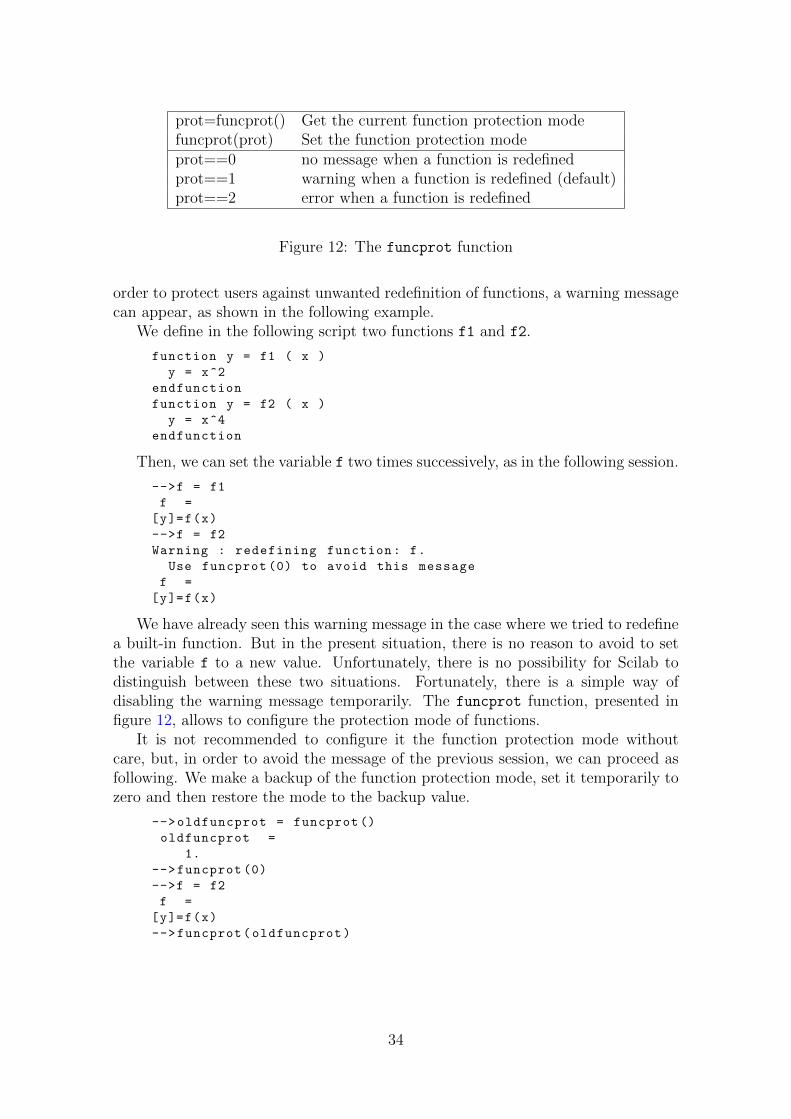
prot=funcprot() Get the current function protection modefuncprot(prot) Set the function protection modeprot==0 no message when a function is redefinedprot==1 warning when a function is redefined (default)prot==2 error when a function is redefined

Figure 12: The funcprot function

order to protect users against unwanted redefinition of functions, a warning messagecan appear, as shown in the following example.

We define in the following script two functions f1 and f2.

function y = f1 ( x )

y = x^2

endfunction

function y = f2 ( x )

y = x^4

endfunction

Then, we can set the variable f two times successively, as in the following session.

-->f = f1

f =

[y]=f(x)

-->f = f2

Warning : redefining function: f.


f =

[y]=f(x)

We have already seen this warning message in the case where we tried to redefinea built-in function. But in the present situation, there is no reason to avoid to setthe variable f to a new value. Unfortunately, there is no possibility for Scilab todistinguish between these two situations. Fortunately, there is a simple way ofdisabling the warning message temporarily. The funcprot function, presented infigure 12, allows to configure the protection mode of functions.

It is not recommended to configure it the function protection mode withoutcare, but, in order to avoid the message of the previous session, we can proceed asfollowing. We make a backup of the function protection mode, set it temporarily tozero and then restore the mode to the backup value.

-->oldfuncprot = funcprot ()

oldfuncprot =

1.

-->funcprot (0)

-->f = f2

f =

[y]=f(x)

-->funcprot(oldfuncprot)

34

3.4 Callbacks

In the following session, we use the derivative function in order to compute thederivative of the function myf. We first define the myf function as squaring its inputarguments x. Then we pass the function myf to the derivative function as a regularinput argument in order to compute the numerical derivative at the point x=2.

-->function y = myf ( x )

--> y = x^2

-->endfunction

-->y = derivative ( myf , 2 )

y =

4.

In order to fully understand the behaviour of callbacks, we can implement ourown numerical derivative function as in the following session. Our implementationof the numerical derivative is based on an order 1 Taylor expansion of the functionin the neighbourhood of the point x. It takes as input arguments the function f,the point x where the numerical derivative is to be computed and the step h whichmust be used.

function y = myderivative ( f , x , h )

y = (f(x+h) - f(x))/h

endfunction

We emphasize that this example is not to be used in practice, since the built-in derivative function is much more powerful than our simplified myderivative

function. This said, notice that, in the body of the myderivative function, theinput argument f is used as a regular function. It is passed successively the inputarguments x+h and x.

Then we pass to the myderivative function the myf argument, which allows tocompute the numerical derivative of our particular function.

-->y = myderivative ( myf , 2 , 1.e-8 )

y =

4.

All in all, although the order 1 Taylor formula is always the same, the myderiva-tive function can be applied to derivate any function which header has the form y

= f(x).

3.5 Protection against wrong uses: warning and error

It often happens that the input arguments of a function can have only a limitednumber of possible values. For example, we might require that a given input doubleis positive, or that a given input floating point integer can have only three values.In this case, we use the error or warning functions, which are presented in figure13.

We now give an example which shows how these functions can be used to protectthe user of a function against wrong uses. In the following script, we define thefunction mynorm, which is a simplified version of the built-in norm function. Ourmynorm function allows to compute the 1, 2 or infinity norm of a vector. In othercases, our function is undefined and this is why we generate an error.

35

error Sends an error message and stops the computation.warning Sends a warning message.gettext Get text translated into the current locale.

Figure 13: The error and warning functions

function y = mynorm ( A , n )

if ( n == 1 ) then

y = sum(abs(A))

elseif ( n == 2 ) then

y=sum(A.^2)^(1/2);

elseif ( n == "inf" ) then

y = max(abs(A))

else

msg = msprintf("%s: Invalid value %d for n.","mynorm",n)

error ( msg )

end

endfunction

In the following session, we test the ouput of the function mynorm when the inputargument n is equal to 1, 2, ”inf” and the unexpected value 12.

-->mynorm ([1 2 3 4],1)

ans =

10.

-->mynorm ([1 2 3 4],2)

ans =

5.4772256

-->mynorm ([1 2 3 4],"inf")

ans =

4.

-->mynorm ([1 2 3 4],12)

!--error 10000

mynorm: Invalid value 12 for n.

at line 10 of function mynorm called by :

mynorm ([1 2 3 4] ,12)

The input argument of the error function is a string. We could have used amore simple message, such as "Invalid value n.", for example. Our message is alittle bit more complicated for the following reason. The goal is to give to the usera useful feedback when the error is generated at the bottom of a complicated chainof calls. In order to do so, we give as much information as possible about the originof the error.

First, it is convenient for the user to be informed about what exactly is the valuewhich is rejected by the algorithm. Therefore, we include the actual value of theinput argument n into the message. Furthermore, we make so that the first stringof the error message is the name of the function. This allows to get immediately thename of the function which is generating the error. The msprintf function is usedin that case to format the string and to produce the msg variable which is passed tothe error function.

We can make so that the error message can be translated into other languages ifnecessary. Indeed, Scilab is localized so that many message appear in the language

36

of the user. In order to do so, we can use the gettext function which returns atranslated string, based on a localization data base. This is done for the previousexample in the following script.

localstr = gettext ( "%s: Invalid value %d for n." )

msg = msprintf ( localstr , "mynorm" , n )

error ( msg )

Notice that the string which is passed to the gettext function is not the outputbut the input of the msprintf function. This is because the localization system isbased on a map from the string "%s: Invalid value %d for n." into localizedstrings such as the translated message "%s: Valeur %d invalide pour n.", infrench for example. These localized messages are stored in ”.pot” data files. A lotmore information about localization is provided at [13].

There are cases when we do want to generate a message, but we do not wantto interrupt the computation. For example, our algorithm might be replaced by abetter one provided in a new version of Scilab. In our particular situation, we maywant to inform our user that the mynorm function is rather poor compared to thebuilt-in norm function. In this case, we do not want to interrupt the algorithm, sincethe computation is perfectly valid and we can use the warning function, as in thefollowing script.

function y = mynorm2 ( A , n )

msg = msprintf("%s: Please use norm instead.","mynorm2" ,1)

warning(msg);

if ( n == 1 ) then

y = sum(abs(A))

elseif ( n == 2 ) then

y=sum(A.^2)^(1/2);

elseif ( n == "inf" ) then

y = max(abs(A))

else

msg = msprintf("%s: Invalid value %d for n.","mynorm2",n)

error ( msg )

end

endfunction

The following session shows the result of the function.

-->mynorm2 ([1 2 3 4],2)

Warning : mynorm2: Please use norm instead.

ans =

5.4772256

3.6 Managing a variable number of arguments

In this section, we present the design of functions with a variable number of input andoutput arguments. As an example, we consider the implementation of a functionwhich computes the numerical derivatives of a given function. The goal of thissection is to present methods which allows to manage a variable number of inputand output arguments. As we are going to see, providing a variable number of inputarguments allows to simplify the use of a function. For example, the function mayprovide to the user default parameters which may increase the numerical accuracy.

37

argn Returns the current number of input and output arguments.varargin A list storing the input arguments.varargout A list storing the output arguments.

Figure 14: Functions related to variable number of input and outpur arguments.

The functions related to this topic are presented in the figure 14.As a brief introduction to the management of the argn function, let us consider

the following script, where we define the myargndemo function.

function varargout = myargndemo ( varargin )

[lhs ,rhs ]=argn()

mprintf("lhs=%d , rhs=%d, length(varargin )=%d\n" ,..

lhs ,rhs ,length(varargin ))

for i = 1 : lhs

varargout(i) = 1

end

endfunction

The varargout and varargin arguments are valid lists which represent the outputand input arguments. In the body of the function definition, we call the argn

function, which produces the two following outputs:

• lhs, the number of output arguments,

• rhs, the number of input arguments.

The varargin variable is defined when the function is called. On the contrary, thetask of defining the varargout variable is left to the function. In our function, wesimply copy the input arguments into the output arguments.

The following session shows how the function performs when it is called.

-->myargndemo ();

lhs=1, rhs=0, length(varargin )=0

-->myargndemo (1);


-->myargndemo (1,2);


-->myargndemo (1,2,3);


-->y1 = myargndemo (1);


-->[y1,y2] = myargndemo (1);


-->[y1,y2,y3] = myargndemo (1);


The previous session shows that the number of elements in the list varargin is rhs.The myargndemo function can be called with any number of input arguments. Inpractice, not all calling sequences will be authorized, so that we will have to inserterror statements which will limit the use of the function.

We now turn to a more practical example, which involves the computation ofnumerical derivatives.

38

The derivative function in Scilab allows to compute the first (Jacobian) andsecond (Hessian) derivatives of a multivariate function. In order to make the discus-sion of this topic more vivid, we consider the problem of implementing a simplifiedversion of this function. The implementation of the derivative function is based onnumerical differenciation and uses finite differences formulas of various orders (see[17] for more details on this subject). The total error which is associated with anyfinite difference formula is the sum of the truncation error (because of the use of alimited number of terms in the Taylor expansion) and a rounding error (because ofthe limited precision of floating point computations in the function evaluation). Itcan be proved that, depending on the finite difference formula used to approximatethe first derivative, there is an optimal step which minimizes the total error. Thisoptimal step depends on the machine precision ε ≈ 10−16, because Scilab uses dou-ble precision floating point numbers. For an order 1 forward finite difference, theoptimal step is h = ε1/2 and for an order 2 centered finite difference, the optimalstep is h = ε1/3.

The following function myderivative1 allows to compute the first derivative ofan univariate function. Its input arguments are the function to differentiate f, thepoint x where the derivative is to be evaluated, the step h and the order order ofthe formula. The function provides an order one forward formula and an order 2centered formula. The output arguments are the value of the first derivative df andthe value of the difference dy.

function [df,dy] = myderivative1 ( f , x , h , order )

if ( order == 1 ) then

y1 = f(x)

y2 = f(x+h)

dy = y2-y1

df = dy/h

else

y1 = f(x-h)

y2 = f(x+h)

dy = y2-y1

df = dy/h

end

endfunction

Notice that the variable dy has no straightforward use in this context, but is pre-sented here for consistency.

As an example, we consider the computation of the numerical derivative of thecosine function at the point x = 0. We define the function myfun, which computesthe cosine of its input argument x.

function y = myfun ( x )

y = cos(x)

endfunction

In the following session, we use the myderivative1 function in order to computethe first derivative of the cosine function.

-->x0 = %pi;

-->order = 1;

-->h = %eps ^(1/2);

-->df = myderivative1 ( myfun , x0 , order , h )

39

df =

7.451D-09

-->h = %eps ^(1/3);

-->order = 2;

-->df = myderivative1 ( myfun , x0 , order , h )

df =

0.

-->[df,dy] = myderivative1 ( myfun , x0 , order , h )

dy =

0.

df =

0.

Since the exact value of the derivative is − sin(0) = 0, we see that the centeredformula, associated with order=2, is, indeed, more accurate.

It would be convenient if we could use default values of the order order andthe step h. For example, we may want to use the default order order=2, since itprovides a more accurate derivative with the same number of function calls. Giventhe order, the optimal step could be computed with either of the formulas h = ε1/2

and h = ε1/3.Hence, the goal of this section is to provide an implementation of the function

which allows to use the following calling sequences.

df = myderivative2 ( myfun , x0 )

df = myderivative2 ( myfun , x0 , order )

df = myderivative2 ( myfun , x0 , order , h )

[df,dy] = myderivative1 ( ... )

The main advantage of this implementation is to be able to provide default valuesfor the input arguments, so that

• the user’s taks is simplified, in the case where he does not want to take thecontrol of the settings,

• all the flexibility of the function is available, since the user can set the param-eters if he wants to.

The following function myderivative2 implements a numerical differenciationalgorithm, with optional order order and step h.

1 function varargout = myderivative2 ( varargin )

2 [lhs ,rhs ]=argn()

3 if ( rhs < 2 | rhs > 4 ) then

4 error ( msprintf (..

5 "%s: Expected %d to %d input arguments , but %d are provided" ,..

6 "myderivative2" ,2,4,rhs))

7 end

8 if ( lhs > 2 ) then

9 error ( msprintf (..

10 "%s: Expected %d to %d output arguments , but %d are provided" ,..

11 "myderivative2" ,0,2,lhs))

12 end

13 f = varargin (1)

14 x = varargin (2)

15 if ( rhs >= 3 ) then

40

16 order = varargin (3)

17 else

18 order = 2

19 end

20 if ( rhs >= 4 ) then

21 h = varargin (4)

22 else

23 if ( order == 1 ) then

24 h = %eps ^(1/2)

25 else

26 h = %eps ^(1/3)

27 end

28 end

29 if ( order == 1 ) then

30 y1 = f(x)

31 y2 = f(x+h)

32 dy = y2-y1

33 df = dy/h

34 else

35 y1 = f(x-h)

36 y2 = f(x+h)

37 dy = y2-y1

38 df = dy/(2*h)

39 end

40 varargout (1) = df

41 if ( lhs >= 2 ) then

42 varargout (2) = dy

43 end

44 endfunction

As the body of this function is quite complicated, we are now going to analyzeits most important parts.

The line #1 defines the function as taking the varargin variable as input argu-ment and the varargout variable as output argument. These are special variablesnames which are considered by the interpreter of Scilab with a particular meaning.Both variables are basic Scilab lists. The varargin variable is a list containingall the variables passed by the user of the function. The number of elements of thislist is the number of elements defined by the user and each item in the list repre-sents an input argument. Inside the body of the function currently being defined,the varargin variable already exists: its content has been pre-set by the Scilabinterpreter. By contrast, the varargout variable is a list which represents theoutput arguments. Its content is not pre-defined by Scilab ; its definition is leftto the developper of the function, who must ensure that the varargout variable isconsistently set at the output of the function. Still, the actual output arguments areset automatically by Scilab, based on the content of the varargout variable. Weemphasize that a function can be defined with both varargin and varargout, withvarargin only or with varargout only: this decision is left to the designer of thefunction.

The line #2 makes use of the argn function, which returns the actual numberof input and output arguments. For example, when the calling sequence df = my-

derivative2 ( myfun , x0 ) is used, we have rhs=2 and lhs=1. The followingscript presents various cases.

41

myderivative2 ( myfun , x0 ) // lhs=1, rhs=2

df = myderivative2 ( myfun , x0 ) // lhs=1, rhs=2

df = myderivative2 ( myfun , x0 , order ) // lhs=1, rhs=3

df = myderivative2 ( myfun , x0 , order , h ) // lhs=1, rhs=4

[df,dy] = myderivative1 ( myfun , x0 ) // lhs=2, rhs=2

The lines #2 to #12 are designed to check that the number of input and outputarguments is correct. For example, the following session shows the error whichis generated in the case where the user wrongly calls the function with 1 inputargument.

-->df = myderivative2 ( myfun )

!--error 10000

myderivative2: Expected from 2 to 4 input arguments , but 1 are provided

at line 6 of function myderivative2 called by :

df = myderivative2 ( myfun )

The lines #13 and #14 shows how to directly set the values of the input argu-ments f and x, which always are forced to be present in the calling sequence. Thelines #15 to #19 allows to set the value of the order parameter. When the numberof input arguments rhs is greater than 3, then we deduce that the value of the ordervariable is given by the user, and we use directly that value. In the opposite case,we set the default value of this parameter, that is we set order=2.

The same processing is done in the lines #17 to #28 in order to set the value ofh. The only thing which changes is that, this time, we use the value of the order

variable in order to set the default value of h.The lines #40 to #43 allows to set the output arguments, thanks to the varar-

gout list. The algorithm depends on the number of output arguments, stored inthe lhs variable. If there are more than one argument, the line #40 is setting thefirst entry of the list, which corresponds to the numerical derivative df. If there aremore than one argument, the lines #41 to #43 are setting the first entry of the list,which corresponds to the function difference dy.

We emphasize that the minimum number of output arguments is 1, so thatwe always have lhs≥ 1. Hence, there is no need to test the value of lhs beforesetting varargout(1). By contrast, the number of output arguments dynamicallydepends on the calling sequence launched by the user of the function. Therefore, itis necessary to test the condition lhs>=2 before setting varargout(2).

The following session shows simple uses of the myderivative2 function. In thefirst call, we use the default value of both order and h. In the second vall, we setthe value of order and use the default value for h.

-->x0 = %pi;

-->df = myderivative2 ( myfun , x0 )

df =

0.

-->order = 1;

-->df = myderivative2 ( myfun , x0 , order )

df =

7.451D-09

We can also call this function with two output arguments, as in the following session.

-->[df,dy] = myderivative2 ( myfun , x0 )

42

dy =

0.

df =

0.

We have seen in this section how to manage a variable number of input andoutput arguments. But the method that we have presented is limited by the orderof the arguments. Indeed, the function myderivative2 cannot be called by usingthe default value for the order argument and setting a customized value for the h

argument.This limitation is caused by the order of the arguments. In practice, it would

be convenient to be able to use the default value of an argument #i, and, still, setthe value of the argument #i+1 (or any other argument on the right of the callingsequence). The next section allows to solve this issue.

3.7 Optional arguments and default values

In this section, we describe how to manage optional arguments with default values.We show how to solve the problem generated with ordered input arguments. Indeed,we saw in the previous paragraph that a basic management of optional argumentsforbid us to set an input argument #i + 1 and use the default value of the inputargument #i. In this section, we present a method where the empty matrix is usedto represent a default parameter.

Let us consider the function myfun, which takes x and p as input arguments andreturns y = q*x p.

function y = myfun ( x , p , q )

y = q*x^p

endfunction

If we both set x, p and q as input arguments, the function performs perfectly, asin the following session.

-->myfun (3,2,1)

ans =

9.

For now, our function myfun is not very flexible, so that if we pass only one ortwo arguments, the function generates an error.

-->myfun (3)

!--error 4

Undefined variable: q

at line 2 of function myfun called by :

myfun (3)

-->myfun (3,2)

!--error 4

Undefined variable: q

at line 2 of function myfun called by :

myfun (3,2)

It would be convenient if the parameter p had the default value 2 and the pa-rameter q had the default value 1. In that case, if neither p nor q are provided, thestatement foo(3) would return 9.

43

But we would also like to be able to set the values of these parameters if thedefault values do not fit. We can use the varargin variable in order to have avariable number of input arguments. But, used directly, this does not allow to setthe third argument and use the default value of the second argument. This issue iscaused because, in Scilab, the input arguments are ordered. In order to solve thisproblem, we are going to use of the empty matrix [].

The idea is the following. First we set the parameter to its default value. Then,depending on the number of input arguments, we overwrite the variable only ifthe argument is different from the empty matrix. This method is presented in thefollowing script.

function y = myfun2 ( varargin )

[lhs ,rhs]=argn ();

if ( rhs <1 | rhs >3 ) then

msg = gettext("%s: Wrong number of input arguments: %d to %d expected .\n")

error(msprintf(msg ,"myfun2" ,1,3))

end

x = varargin (1)

p = 2

if ( rhs >= 2 ) then

if ( varargin (2) <> [] ) then

p = varargin (2)

end

end

q = 1

if ( rhs >= 3 ) then

if ( varargin (3) <> [] ) then

q = varargin (3)

end

end

y = q * x^p

endfunction

The major advantage of the previous method is to be able to use the defaultvalue of the argument p, while setting the value of the argument q. This situationis illustrated in the following session. To do so, we simply set the argument p to theempty matrix, as in the following session.

-->myfun2 (2,[],3)

ans =

12.

Of course, we can still use the optional arguments as usual, which is presentedin the following session.

-->myfun2 (2)

ans =

12.

-->myfun2 (2,3)

ans =

24.

-->myfun2 (2,3,2)

ans =

16.

44

In practice, this method is both flexible and consistent with the basic manage-ment of input arguments, which is mainly based on their order.

This method is still of limited simplicity if the number of input arguments islarge. In this case, there are other solutions which allow to avoid to use orderedarguments. In the next sections, we will analyse the parameters module, whichallow to configure an unordered set of input arguments separately from the actualuse of the parameters. Emulating object oriented programming is another method,which is extremely flexible thanks to the use of a specialized configure function.

3.8 Functions with variable type input arguments

We often have the situation where it would be convenient to have a single functionperform two (or more) different treatments depending on the type of data to process.The following function illustrates this situation, when we want to have a particulardisplay of a matrix of doubles, and another printing with boolean matrices. Thebody of the function is based on a if statement, which switches to different part ofthe source code depending on the type of the X variable.

function myprint ( X )

if ( type(X) == 1 ) then

disp("Double matrix")

elseif ( type(X) == 4 ) then

disp("Boolean matrix")

else

error ( "Unexpected type." )

end

endfunction

In the following session, we call the myprint function with two different types ofmatrices.

->myprint ( [1 2] )

Double matrix

-->myprint ( [%T %T] )

Boolean matrix

We can make the previous function more useful, by defining separate formattingrules used to print the data, as in the following function.

function myprint ( X )

if ( type(X) == 1 ) then

// Real matrix

for i = 1 : size(X,"r")

for j = 1 : size(X,"c")

mprintf("%-5d ",X(i,j))

if ( j == 3 ) then

mprintf(" ")

end

end

mprintf("\n")

end

elseif ( type(X) == 4 ) then

// Boolean matrix

for i = 1 : size(X,"r")

45

for j = 1 : size(X,"c")

mprintf("%s ",string(X(i,j)))

if ( j == 3 ) then

mprintf(" ")

end

end

mprintf("\n")

end

else

error ( "Unexpected type for input argument var." )

end

endfunction

The following session gives a sample use of the previous function.

-->X = [

-->1 2 3 4 5 6

-->7 8 9 10 11 12

-->13 14 15 16 17 18

-->];

-->

-->myprint ( X )

1 2 3 4 5 6

7 8 9 10 11 12

13 14 15 16 17 18

-->

-->X = [

-->%T %T %F %F %F %F

-->%T %F %F %T %T %T

-->%F %T %F %F %T %F

-->];

-->

-->myprint ( X )

T T F F F F

T F F T T T

F T F F T F

3.9 Using parameters

The goal of the parameters module is to be able to design a function which hasa possibly large amount of optional parameters. Using this module allows to avoidto design a function with a large number of input arguments, which may lead toconfusion. This module has been introduced in Scilab v5.0, after the work by YannCollette to integrate optimization algorithms such as Genetic Algorithms and Sim-ulated Annealing. The functions of the parameters module are presented in thefigure 15.

In the first section, we make an overview of the module and describe its direct use.In the second section, we present a practical example, based on a sorting algorithm.The last section focuses on the safe use of the module, protecting the user againstcommon mistakes.

46

add_param Add a parameter to a list of parametersget_param Get the value of a parameter in a parameter listinit_param Initialize the structure which will handles the parameters listis_param Check if a parameter is present in a parameter listlist_param List all the parameters name in a list of parametersremove_param Remove a parameter and its associated value from a list of parametersset_param Set the value of a parameter in a parameter list

Figure 15: Functions from the parameters module.

3.9.1 Overview of the module

In this section, we present the parameters module and give an example of its use,in the context of a merge-sort algorithm.

In order to understand the parameters module, we can separate the situationbetween two points of view:

• the user’s point of view,

• the developer’s point of view.

Therefore, in the following discussion, we will discuss first what happens when wewant to use the parameters module in order to call a function. Then, we will discusswhat the developer has to do in order to manage the optional parameters.

In order to make the discussion as applied as possible, we will take an exampleand will examine it throuhought this section.

We consider a function mergesort, which defines a sorting algorithm based on acombination of recursive sorting and merging. The mergesort function is associatedwith the following calling sequences, where x is a matrix of doubles to be sorted,params is a list of parameters and y is a matrix of sorted doubles.

y = mergesort ( x )

y = mergesort ( x , params )

The actual implementation of the mergesort function will be defined later in thissection. The params variable is a list of parameters which defines two parameters:

• direction, a boolean which is true for increasing order and false for decreasingorder,

• compfun, a function which defines a comparison function.

We now present a simple use of the functions from the parameters module.Assume that we have a function which has the optional parameter direction, withthe default value %t. In the following script, we call the init_param function, whichcreates the empty list of parameters params. Then, we add the key "direction"

to the list of parameters.

params = init_param ();

params = add_param(params ,"direction",%f);

47

At this point, we assume that the user calls a function using the input argumentparams.

x = [4 5 1 6 2 3]’;

y = mergesort ( x , params );

We are now going to analyze what statements may be used in the body of themergesort function. In the following session, we call the get_param function inorder to get the value corresponding to the key "direction". We pass the %t valueto the get_param function, in order to express that this is the default value in thecase where this key is not defined.

-->direction = get_param(params ,"direction",%t)

direction =

F

Since the "direction" key is defined and is false, we simply get back our value. Wemay use an extended calling sequence of the get_param function, with the outputargument err. The err is true if an error has occured during the processing of theargument.

-->[direction ,err] = get_param(params ,"direction",%t)

err =

F

direction =

F

In our case, no error is produced and this is why the variable err is false.As we have seend, the technic is based on a mapping from keys to values. Each

key corresponds to a field of the list of parameters and is stored as a string. Thetype of each value depends on the particular requirements of the algorithm.

We can analyze other combinations of events. For example, Let us consider thesituation where the user defines only an empty list of parameters, as in the followingscript.

params = init_param ();

In this case, a straightforward call to the get_param function generates a warn-ing.


WARNING: get_param: parameter direction not defined

direction =

T

The warning indicates that the "direction" key is not defined, so that the defaultvalue %t is returned. If we use the additionnal output argument err, there is nowarning anymore, but the err variable becomes true.


err =

T

direction =

T

As a last example, let us consider the case where the user defines the params

variable as an empty matrix.

48

params = [];

As we are going to see later in this section, this case may happen when we want touse the default values. The following session shows that an error is generated whenwe call the get_param function.


!--error 10000

get_param: Wrong type for input argument #1: plist expected.

at line 40 of function get_param called by :

direction = get_param(params ,"direction",%t)

Indeed, the variable params is expected to be a plist. This is because the init_paramfunction creates variables with type plist, which stands for ”parameters list”. Infact, the actual implementation of the init_param function creates a typed list withtype plist. In order to avoid to generate the previous error, we can use the err

output argument, as in the following session.


err =

T

direction =

T

We see that the err variable is true, indicating that an error has been detectedduring the processing of the variable params. As before, in this case, the get_param

function returns the default value.

3.9.2 A practical case

In this section, we consider the actual implementation of the mergesort function pre-sented in the previous section. The sorting algorithm that we are going to presentis based on an algorithm designed by Bruno Pincon in 2008, ”Quelques tests derapidite entre differents logiciels matriciels”. The modifications included in the im-plementation presented in this section include the management of the "direction"

and "compfun" optional arguments. Interested readers will find many details aboutsorting in [12].

The following mergesort function provides a sorting algorithm, based on amerge-sort method. Its first argument is x, that is, the matrix of doubles to besorted. The second argument, params, is optional and represents the list of param-eters. We make a first call to the get_param function in order to get the value ofthe direction parameter, with %t as the default value. Then we get the value ofthe compfun parameter, with compfun_default as the default value. The comp-

fun_default function is defined later in this section. Finally, we call the merge-

sortre function, which actually implements the recursive merge-sort algorithm.

function y = mergesort ( varargin )

[lhs ,rhs]=argn()

if ( and( rhs <>[1 2] ) ) then

errmsg = sprintf (..

"%s: Unexpected number of arguments : " + ..

"%d provided while %d to %d are expected." ,..

"mergesort",rhs ,1,2);

49

error(errmsg)

end

x = varargin (1)

if ( rhs <2 ) then

params = []

else

params = varargin (2)

end

[direction ,err] = get_param(params ,"direction",%t)

[compfun ,err] = get_param(params ,"compfun",compfun_default)

y = mergesortre ( x , direction , compfun )

endfunction

The following mergesortre function implements the recursive merge-sort algorithm.The algorithm divides the matrix x into two even parts x(1:m) and x(m+1:n). Oncesorted by a recursive call into x1 and x2, we merge the two sub-parts back into x.

function x = mergesortre ( x , direction , compfun )

n = length(x)

indices = 1 : n

if ( n > 1 ) then

m = floor(n/2)

p = n-m

x1 = mergesortre ( x(1:m) , direction , compfun )

x2 = mergesortre ( x(m+1:n) , direction , compfun )

x = merge ( x1 , x2 , direction , compfun )

end

endfunction

The following merge function merges its two sorted input arguments x1 and x2

into its sorted output argument x. The comparison operation is performed by thecompfun function, which returns -1, 0 or 1 depending on the comparison betweenits two input arguments. In the case where the direction argument is false, weinvert the sign of the order variable, so that the order is ”decreasing” instead of thedefault ”increasing” order.

function x = merge ( x1 , x2 , direction , compfun )

n1 = length(x1)

n2 = length(x2)

n = n1 + n2

x = []

i = 1

i1 = 1

i2 = 1

for i = 1:n

order = compfun ( x1(i1) , x2(i2) )

if ( ~direction ) then

order = -order

end

if ( order <=0 ) then

x(i) = x1(i1)

i1 = i1+1

if (i1 > m) then

x(i+1:n) = x2(i2:p)

break

end

50

else

x(i) = x2(i2)

i2 = i2+1

if (i2 > p) then

x(i+1:n) = x1(i1:m)

break

end

end

end

endfunction

We notice that the mergesort function does not call itself. Instead, the merge-

sortre function, which actually performs the algorithm recursively, has fixed inputarguments. This allows to reduce the overhead caused by the processing of theoptional arguments.

The following compfun_default function is the default comparison function. Itreturns order=-1 if x<y, order=0 if x==y and order=1 if x>y.

function order = compfun_default ( x , y )

if ( x < y ) then

order = -1

elseif ( x==y ) then

order = 0

else

order = 1

end

endfunction

We now analyze the behaviour of the mergesort function by calling it withparticular inputs. In the following session, we sort the matrix x containing floatingpoint integers. As we can see, the mergesort sorts the matrix by increasing order.

-->x = [4 5 1 6 2 3]’;

-->mergesort ( x )

ans =

1.

2.

3.

4.

5.

6.

In the following session, we configure the direction parameter to %f, so that theorder of the sorted matrix is ”decreasing”.

-->params = init_param ();

-->params = add_param(params ,"direction",%f);

-->mergesort ( x , params )

ans =

6.

5.

4.

3.

2.

1.

51

We now want to customize the comparison function, so that we can changethe order of the sorted matrix. In the following session, we define the comparisonfunction mycompfun which allows to separate even and odd floating point integers.

function order = mycompfun ( x , y )

if ( modulo(x,2) == 0 & modulo(y,2) == 1 ) then

// even < odd

order = -1

elseif ( modulo(x,2) == 1 & modulo(y,2) == 0 ) then

// odd > even

order = 1

else

// 1<3, or 2<4

if ( x < y ) then

order = -1

elseif ( x==y ) then

order = 0

else

order = 1

end

end

endfunction

We can configure the params variable so that the sort function uses our customizedcomparison function mycompfun instead of the default comparison function comp-

fun_default.


-->params = add_param(params ,"compfun",mycompfun );

-->mergesort ( [4 5 1 6 2 3]’ , params )

ans =

2.

4.

6.

1.

3.

5.

We do not configure the direction parameter, so that the default ”increasing”orderis used. As we can see, in the output argument, the even numbers are before theodd numbers, as expected.

3.9.3 Issues with the parameters module

There is an issue with the parameters module, which may make the user considerdefault values instead of the expected ones. All in all, the parameters module doesnot protect against unexpected fields, which may happen if we make a mistake inthe name of the key when we configure a parameter.

In the following session, we call the function with the wrong key ”compffun”instead of ”compfun”.


-->params = add_param(params ,"compffun",mycompfun );


ans =

52

1.

2.

3.

4.

5.

6.

We see that our function mycompfun has been ignored, so that the default comparisonfunction is used instead. The reason behind this is that the parameters module doesnot check that the ”compffun” function is unexpected.

This is why we suggest to use the following check_param function, which takes asintput arguments the list of parameters params and a matrix of strings allkeys. Theallkeys variable is expected to store the complete list of keys which are availablein the list of parameters. The algorithm checks that each key in params is presentin allkeys. The output arguments are a boolean noerr and a string msg. If thereis no error, the noerr is true and the string msg is an empty matrix. If one keyof params is not found, we set noerr to false and compute an error message. Thiserror message is used to actually generate an error only if the output argument msgwas not used in the calling sequence.

function [noerr ,msg] = check_param(params ,allkeys)

currkeys = getfield(1,params)

nkeys = size(currkeys ,"*")

noerr = %t

msg = []

// The key #1 is "plist".

for i = 2 : nkeys

k = find(allkeys == currkeys(i))

if ( k == [] ) then

noerr = %f

msg = msprintf (..

gettext("%s: Unexpected key ""%s"" in parameter list."),..

"check_param",currkeys(i))

if ( lhs < 2 ) then

error ( msg )

end

break

end

end

endfunction

The following version of the mergesort function uses the check_param state thatthe list of available keys is the matrix ["direction" "compfun"].

function y = mergesort ( varargin )

[lhs ,rhs]=argn()

if ( and( rhs <>[1 2] ) ) then

errmsg = sprintf (..

"%s: Unexpected number of arguments : "+..

"%d provided while %d to %d are expected." ,..

"mergesort",rhs ,1,2);

error(errmsg)

end

x = varargin (1)

if ( rhs <2 ) then

53

params = []

else

params = varargin (2)

end

check_param(params ,["direction" "compfun"])

[direction ,err] = get_param(params ,"direction",%t)

[compfun ,err] = get_param(params ,"compfun",compfun_default)

y = mergesortre ( x , direction , compfun )

endfunction

In the following session, we use, as previously, the wrong key ”compffun” insteadof ”compfun”.


-->params = add_param(params ,"compffun",mycompfun );


!--error 10000

check_param: Unexpected key "compffun" in parameter list.

at line 75 of function check_param called by :

at line 16 of function mergesort called by :

mergesort ( [4 5 1 6 2 3]’ , params )

With our fixed function, an error message is generated, which allows to see ourmistake.

3.10 Issues with callbacks

TODO : issues with callbacks - interactions with user’s defined function names (voirbugs 7102, 7103, 7104)

3.11 Callbacks with additionnal arguments

TODO : callbacks avec arguments supplementaires : list(f,2) > exercise

3.12 Robust functions

TODO : rules for robust functions : arg number, type, size and contentTODO : the apifun external module

3.13 Exercises

Exercise 3.1 () (Maximum stack size) What is the maximum size of the stack on your currentmachine ?

TODO : Comment faire un tri avec un ordre particulier sur les complexes ?

4 Performances

In this section, we present a set of Scilab programming skills which allow to producescripts which are fast. These methods are known as vectorization and is at the coreof most efficient Scilab functions. Because fast performances is a central concernwhen we develop a script, we will show how to measure

54

tic, toc measure user timetimer measure system time

Figure 16: Performance functions.

The figure 16 presents some Scilab functions which are used in the context ofanalysing the performance of a Scilab script.

4.1 Measuring the performance

In this section, we describe the functions which allow to measure the time required bya computation. Indeed, before optimizing any program, we must precisely measureits current performances.

In order to measure the time required by a computation, we can use the tic andtoc functions which measure the user time in seconds. The user time is the wallclock time, that is, the time that was required by the computer from the start ofthe task to its end, including the computation itself, of course, but also all otheroperations of the system, like refreshing the screen, updating the file system, lettingother process do a part of their work, etc... In the following session, we use the tic

and toc to measure the time to compute the eigenvalues of a random matrix, basedon the spec function.

-->tic(); lambda = spec(rand (200 ,200)); t = toc()

t =

0.1

The call to the tic starts the counter and the call to the toc function stops it,returning the number of elapsed seconds. In this case, we typed the statements onthe same line, using the ; separator: indeed, if we typed the instructions interactivelyon several lines, the measured time would mainly be the time required by the typing(in my case, this requires approximately 20 seconds!).

The previous time measure is not very reliable in the sense that if we performthe same statements several times, we do not get the same time. The following isan example of this behavior.


t =

0.18


t =

0.19

A possible solution for this problem is to perform the same computation severaltimes, say 10 times for example, and to average the results. In the following script,we perform the same computation 10 times, and then display the minimum, themaximum and the average.

for i = 1 : 10

tic();

lambda = spec(rand (200 ,200));

t(i) = toc();

55

end

min(t)

max(t)

mean(t)


-->min(t)

ans =

0.1

-->max(t)

ans =

0.13

-->mean(t)

ans =

0.1081

If another program on the computer uses the CPU at the same time that Scilabperforms its computation, the user time may increase. Therefore, the tic and toc

functions are not used in situations where timing accuracy matters. Indeed, mostof the time, the user time is not what we want to measure. We can use insteadthe timer function which measure the system time, which corresponds to the timerequired by the CPU to actually perform the specific computation required by Scilab.This allows to measure the time consumed by Scilab, and not by other processes.

The following script presents an example of use of the timer function.

for i = 1 : 10

timer ();

lambda = spec(rand (200 ,200));

t(i) = timer ();

end

min(t)

max(t)

mean(t)


-->min(t)

ans =

0.100144

-->max(t)

ans =

0.1101584

-->mean(t)

ans =

0.1021469

4.2 An example of performance analysis

Assume that we are given a column vector and that we want to compute the meanof the values of this vector of data. We have two possibilities to perform this task:

• use the mean function,

• create our own algorithm.

56

In a practical situation, of course, the problem might be far more complicated andmay require a function which is not provided directly by Scilab. For the sake ofsimplicity, we will consider here a situation where the algorithm is elementary. Still,we will see in this section the differences of performances between a naive algorithmand an efficient algorithm, based on vectorization principles.

The following function computes the mean of the input vector v by performinga loop on the data and computing a cumulated sum.

// A naive average , based on a slow loop

function y = mynaivemean ( v )

y = 0;

n = length(v);

for i = 1:n

y = y + v(i);

end

y = y / n;

endfunction

The function mynaivemean encapsulates the algorithm, which will allow us to mea-sure its performances more easily. Before optimizing our algorithm, we check thatit performs its task correctly: indeed, it would be a loss of time to make faster analgorithm which is not correct... The algorithm seems to be correct, as shown bythe following session.

-->y = mynaivemean (1:9)

y =

5.

In order to test our algorithm, we create want to generate large input vectors v.For this purpose, we will use the rand function, because we know that our algorithmdoes not depends on the actual values of the input vector. We emphasize this detail,because practical algorithm may exhibit faster or slower performances depending ontheir input parameters. This is not the case here, so that our analysis is simplified.We generate vectors with size n = 10j with j = 1, 2, . . . , 6. To generate the integersn, we use the logspace function, which returns values following a logarithmic rule.The following script performs a loop from n = 101 up to n = 106 and measure thetime required by our naive algorithm. rand function

n_data = logspace (1,6,6);

for i = 1:6

n = n_data(i);

v = rand(n,1);

timer ();

ymean = mynaivemean ( v );

t = timer ();

mprintf ("i=%d, N=%d , mean=%f, t=%f\n", i , n , ymean , t );

end


i=1, N=10, mean =0.503694 , t=0.000000

i=2, N=100, mean =0.476163 , t=0.000000

i=3, N=1000, mean =0.505503 , t=0.010014

i=4, N=10000 , mean =0.500807 , t=0.090130

i=5, N=100000 , mean =0.499590 , t=0.570821

i=6, N=1000000 , mean =0.500216 , t=5.257560

57

We see that the time grows very fast and is quite large for n = 106.It is in fact possible to get a much faster algorithm. For example, consider the

performance of the mean function.

i=1, N=10, mean =0.493584 , t=0.000000

i=2, N=100, mean =0.517783 , t=0.000000

i=3, N=1000, mean =0.484507 , t=0.000000

i=4, N=10000 , mean =0.501106 , t=0.000000

i=5, N=100000 , mean =0.502038 , t=0.000000

i=6, N=1000000 , mean =0.499698 , t=0.010014

As we see, the mean function is much faster than our mynaivemean function.In order to improve our algorithm, we can use the sum function, which returns

the sum of the elements of its input argument. The following myfastmean functionperforms the computation based on the sum function.

function y = myfastmean ( v )

y = sum(v);

n = length(v);

y = y / n;

endfunction

The following session presents the performance of our improved function.

i=1, N=10, mean =0.419344 , t=0.000000

i=2, N=100, mean =0.508345 , t=0.000000

i=3, N=1000, mean =0.501551 , t=0.000000

i=4, N=10000 , mean =0.501601 , t=0.000000

i=5, N=100000 , mean =0.499188 , t=0.000000

i=6, N=1000000 , mean =0.499992 , t=0.010014

The performance of our fast function is now approximately the same as the perfor-mance of the built-in mean function. In fact, the mean function is a macro, whichperforms mainly the same algorithm as our function, that is, it uses the sum function.Moreover, the mean functions takes into account for several additional options andcan manage various shape of input matrices (row vectors, column vectors or generalmatrices).

TODO : introduce the benchfun function.

function [t,msg] = benchfun ( name , fun , iargs , nlhs , kmax )

//

// Compute the intstruction string to be launched

ni = length ( iargs )

instr = ""

// Put the LHS arguments

instr = instr + "["

for i = 1 : nlhs

if ( i > 1 ) then

instr = instr + ","

end

instr = instr + "x" + string(i)

end

instr = instr + "]"

// Put the RHS arguments

instr = instr + "=fun("

for i = 1 : ni

if ( i > 1 ) then

58

instr = instr + ","

end

instr = instr + "iargs("+string(i)+")"

end

instr = instr + ")"

//

// Loop over the tests

for k = 1 : kmax

// Call the function

timer()

ierr = execstr ( instr , "errcatch" )

t(k) = timer()

end

msg = msprintf("%s: %d iterations , mean=%f, min=%f, max=%f\n",name ,kmax ,mean(t),min(t),max(t))

mprintf("%s\n",msg)

endfunction

4.3 The interpreter

In this section, we briefly present compilation methods so that we can have clearideas about the consequences of the interpreter for performances issues.

Consider the following Scilab script.

y = f(x)

In the previous script, we assume that the variable x is well defined (say a double,for example), that the function f takes one input argument and returns the outputargument y. Most of the time, we are not aware of the high level of complexity whichis hidden behind these simple statements. In order to understand what exactlyhappens when these statements are executed, we must take a look at the structureof a compiler.

A compiler[4] is a program that can read a program in one language and translateit into an equivalent program. If the target program is an executable written inmachine language, it call be called by the user to process inputs and produce outputs.Typical compilers of this type are the Fortran and C/C++ compilers (among others).

Contrary to the previous scheme, Scilab is not a compiled language, it is aninterpreter. Instead of producing a machine-language program, Scilab both uses thesource program and the input data and directly produces the output. The figure17 presents an interpreter. Typical interpreter of this type are Scilab, Matlab andPython (among others).

The machine-language program produced by a compiler is generally faster thatan interpreter at mapping inputs to outputs. An interpreter, however, can usuallygive better diagnostics than a compiler, because it executes the source programstatement by statement.

A compiler is typically structured as a sequence of operations. The first oper-ation involves reading the characters of the source code and performs the lexicalanalysis. This step consists in grouping the characters into meaningful sequencescalled lexemes. The tokens are then passed to the syntax analyzer (or parser), whichuses the tokens and creates a tree representation of the source, which is associated tothe grammatical structure of the source. In the semantic analysis, the compiler uses

59

InterpreterSource Program

Input

Output

Figure 17: Scilab is an interpreter

Script Gateway LibraryInterpreter

Figure 18: Scilab connects the interpreter to a collection of libraries, via gateways.

the syntax tree and check the source for consistency with the language definition.This step involves checking the types of the operands of each operator.

Several intermediate operations may then be involved, leading to the final callto a library routine. In Scilab, this final step is implemented in gateways. Indeed,each Scilab function or operator is uniquely associated with a computational rou-tine implemented in a compiled language, generally in C or Fortran. The gatewayreads the input arguments, check their types and consistency, performs the requiredcomputations, and then push back the output arguments into the interpreter. Thisstructure is presented in figure 18.

Consider now the following two scripts, which perform exactly the same com-putation, namely, the sum of the n = 5 numbers, stored in the following variablex.

x=[1 2 3 4 5];

The following script calls the sum.

y = sum(x);

This requires only one call to the interpreter and involves only one call to oneparticular gateway.

The following script performs the same computation, with a loop.

y = 0;

n = size(x,"*");

for i = 1 : n

y = y + x(i);

end

The previous script involves the interpreter at least n = 5 times, that is, one for eachitem in the loop (plus, may be, some additional calls, for example to compute thevector 1 : n). When n is large, the extra cost of using a loop instead of a vectorizedstatement is very expensive. This is why using vectorized statements is much fasterthat using loops.

60

But there is more, because Scilab uses optimized libraries, which makes an ef-ficient use of the processor. This is the topic covered in the next section, whichpresent several libraries used in Scilab.

4.4 BLAS, LAPACK, ATLAS and the MKL

In this section, we briefly present the BLAS, LAPACK, ATLAS and MKL libraries,in order to have a global overview on these libraries. These libraries are used byScilab in order to provide maximum performances on each system.

The BLAS (Basic Linear Algebra Subprograms) library [2] is a collection ofFortran routines providing low level operations such as vector additions, dot productsand matrix - matrix multiplications. The BLAS library is divided in three levels.

• The Level 1 BLAS perform scalar, vector and vector-vector operations.

• The Level 2 BLAS perform matrix-vector operations.

• The Level 3 BLAS perform matrix-matrix operations.

The LAPACK (Linear Algebra Package) library [3] is a collection of Fortranroutines for solving high level linear algebra problems. This includes solving systemsof simultaneous linear equations, least-square solutions of linear systems, eigenvalueproblems and singular value problems.

The ATLAS (Automatically Tuned Linear Algebra Software) library [1] is alibrary which provides optimized linear algebra BLAS routines and a small subset ofLAPACK optimized routines. The library focus on applying empirical techniques inorder to provide portable performance. The ATLAS library provides in many casessensible performance improvements over a ”basic” BLAS/LAPACK system.

The Intel Math Kernel Library [11] is a library of highly optimized, extensivelythreaded math routines for science, engineering, and financial applications that re-quire maximum performance. This library is developed by Intel and optimizes theperformances of the algorithms specifically for Intel CPUs. Scilab currently usesonly the linear routines of the MKL, in replacement of BLAS.

On Windows, it is advised that user select the Intel MKL for installation. OnLinux systems, optimized version of the ATLAS library are used. Scilab develop-ers compile various optimized version of the ATLAS library, on the various Linuxplatforms where Scilab is distributed.

The main reason for the performance boost of vectorized functions is that Scilabis able to perform the computation on a collection of data, instead of processingeach computation separately. Indeed, the performance of a computation is largelydriven by the fact that the CPU can access to the data which is available in varioustypes of memories that are associated with it. From the fastest to the slowest, thememories used in modern computers are the various levels of cache (built in theprocessor itself) and the Random Access Memory (RAM) (we do not consider herethe hard drive as a memory unit, although it is involved in the management of thevirtual memory). The figure 19 presents the various levels of memories typicallyused by a computer.

61

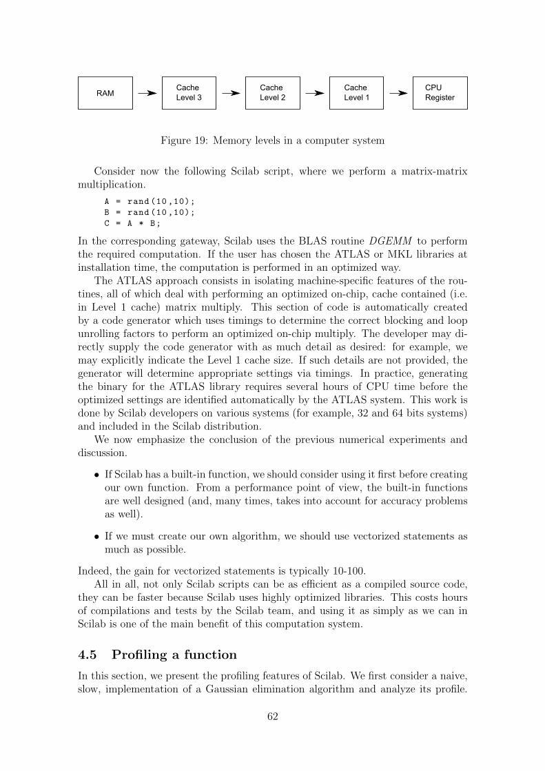
CPURegister

CacheLevel 1

CacheLevel 2

CacheLevel 3RAM

Figure 19: Memory levels in a computer system

Consider now the following Scilab script, where we perform a matrix-matrixmultiplication.

A = rand (10 ,10);

B = rand (10 ,10);

C = A * B;

In the corresponding gateway, Scilab uses the BLAS routine DGEMM to performthe required computation. If the user has chosen the ATLAS or MKL libraries atinstallation time, the computation is performed in an optimized way.

The ATLAS approach consists in isolating machine-specific features of the rou-tines, all of which deal with performing an optimized on-chip, cache contained (i.e.in Level 1 cache) matrix multiply. This section of code is automatically createdby a code generator which uses timings to determine the correct blocking and loopunrolling factors to perform an optimized on-chip multiply. The developer may di-rectly supply the code generator with as much detail as desired: for example, wemay explicitly indicate the Level 1 cache size. If such details are not provided, thegenerator will determine appropriate settings via timings. In practice, generatingthe binary for the ATLAS library requires several hours of CPU time before theoptimized settings are identified automatically by the ATLAS system. This work isdone by Scilab developers on various systems (for example, 32 and 64 bits systems)and included in the Scilab distribution.

We now emphasize the conclusion of the previous numerical experiments anddiscussion.

• If Scilab has a built-in function, we should consider using it first before creatingour own function. From a performance point of view, the built-in functionsare well designed (and, many times, takes into account for accuracy problemsas well).

• If we must create our own algorithm, we should use vectorized statements asmuch as possible.

Indeed, the gain for vectorized statements is typically 10-100.All in all, not only Scilab scripts can be as efficient as a compiled source code,

they can be faster because Scilab uses highly optimized libraries. This costs hoursof compilations and tests by the Scilab team, and using it as simply as we can inScilab is one of the main benefit of this computation system.

4.5 Profiling a function

In this section, we present the profiling features of Scilab. We first consider a naive,slow, implementation of a Gaussian elimination algorithm and analyze its profile.

62

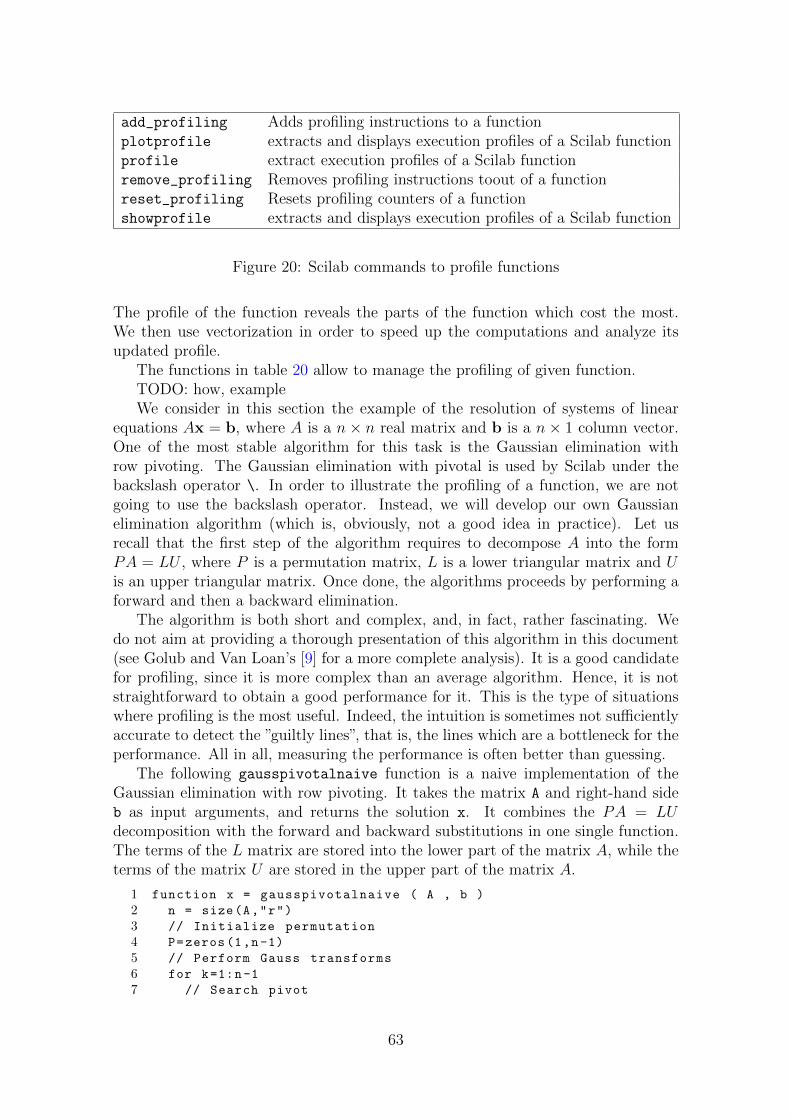
add_profiling Adds profiling instructions to a functionplotprofile extracts and displays execution profiles of a Scilab functionprofile extract execution profiles of a Scilab functionremove_profiling Removes profiling instructions toout of a functionreset_profiling Resets profiling counters of a functionshowprofile extracts and displays execution profiles of a Scilab function

Figure 20: Scilab commands to profile functions

The profile of the function reveals the parts of the function which cost the most.We then use vectorization in order to speed up the computations and analyze itsupdated profile.

The functions in table 20 allow to manage the profiling of given function.TODO: how, exampleWe consider in this section the example of the resolution of systems of linear

equations Ax = b, where A is a n× n real matrix and b is a n× 1 column vector.One of the most stable algorithm for this task is the Gaussian elimination withrow pivoting. The Gaussian elimination with pivotal is used by Scilab under thebackslash operator \. In order to illustrate the profiling of a function, we are notgoing to use the backslash operator. Instead, we will develop our own Gaussianelimination algorithm (which is, obviously, not a good idea in practice). Let usrecall that the first step of the algorithm requires to decompose A into the formPA = LU , where P is a permutation matrix, L is a lower triangular matrix and Uis an upper triangular matrix. Once done, the algorithms proceeds by performing aforward and then a backward elimination.

The algorithm is both short and complex, and, in fact, rather fascinating. Wedo not aim at providing a thorough presentation of this algorithm in this document(see Golub and Van Loan’s [9] for a more complete analysis). It is a good candidatefor profiling, since it is more complex than an average algorithm. Hence, it is notstraightforward to obtain a good performance for it. This is the type of situationswhere profiling is the most useful. Indeed, the intuition is sometimes not sufficientlyaccurate to detect the ”guiltly lines”, that is, the lines which are a bottleneck for theperformance. All in all, measuring the performance is often better than guessing.

The following gausspivotalnaive function is a naive implementation of theGaussian elimination with row pivoting. It takes the matrix A and right-hand sideb as input arguments, and returns the solution x. It combines the PA = LUdecomposition with the forward and backward substitutions in one single function.The terms of the L matrix are stored into the lower part of the matrix A, while theterms of the matrix U are stored in the upper part of the matrix A.

1 function x = gausspivotalnaive ( A , b )

2 n = size(A,"r")

3 // Initialize permutation

4 P=zeros(1,n-1)

5 // Perform Gauss transforms

6 for k=1:n-1

7 // Search pivot

63

8 mu = k

9 abspivot = abs(A(mu,k))

10 for i=k:n

11 if (abs(A(i,k))>abspivot) then

12 mu = i

13 abspivot = abs(A(i,k))

14 end

15 end

16 // Swap lines k and mu from columns k to n

17 for j=k:n

18 tmp = A(k,j)

19 A(k,j) = A(mu,j)

20 A(mu,j) = tmp

21 end

22 P(k) = mu

23 // Perform transform for lines k+1 to n

24 for i=k+1:n

25 A(i,k) = A(i,k)/ A(k,k)

26 end

27 for i = k+1:n

28 for j = k+1:n

29 A(i,j) = A(i,j) - A(i,k) * A(k,j)

30 end

31 end

32 end

33 // Perform forward substitution

34 for k=1:n-1

35 // Swap b(k) and b(P(k))

36 tmp = b(k)

37 mu = P(k)

38 b(k) = b(mu)

39 b(mu) = tmp

40 // Substitution

41 for i=k+1:n

42 b(i) = b(i) - b(k) * A(i,k)

43 end

44 end

45 // Perform backward substitution

46 for k=n:-1:1

47 t = 0.

48 for j=k+1:n

49 t = t + A(k,j) * b(j)

50 end

51 b(k) = (b(k) - t) / A(k,k)

52 end

53 x = b

54 endfunction

Before actually measuring the performance, we must test for correctness, sincethere is no point at making faster a function which has bugs. That seems obvious, butit is often neglected in practice. In the following session, we generate a 10×10 matrixA with entries uniform in [0, 1]. We selected this test case for its very small conditionnumber. We select the expected solution e as being equal to one and compute theright-hand side b from the equation b=A*e. Finally, we use our gausspivotalnaivefunction to compute the solution x.

64

n = 10;

A = grand(n,n,"def");

e = ones(n,1);

b = A * e;

x = gausspivotalnaive ( A , b );

Then, we check that the condition number of the matrix is not too large. Inthe following session, we compute the 2-norm condition number of the matrix A andcheck that is is close to 101, which is rather small. We also check that the relativeerror on x has the same magnitude as %eps≈ 10−16, which is the best that we canhope.

-->log10(cond(A))

ans =

1.3898417

-->norm(e-x)/norm(e)

ans =

6.455D-16

A more complete testing would be required, but we now assume that we can trustour function.

In the following session, we call the add_profiling function in order to profilethe gausspivotalnaive function.

-->add_profiling("gausspivotalnaive")

Warning : redefining function: gausspivotalnaive .


The goal of the add_profiling function is to redefine the function to be profiled,so that Scilab can store the number of times that each line has been executed. Asindicated by the warning, this actually modifies the profiled function, making itslower. Hopefully, we assume that the modified, function has the same profile thatthe original one, but this may depend on the particular situation.

In order to measure the performance of our function, we must execute it, as inthe following session.

x = gausspivotalnaive ( A , b );

Now that sufficient data has been gathered by the profiling system, we are readyto analyze it. In the following script, we call the plotprofile function in order toplot a graphics displaying the profile of the function.

plotprofile(gausspivotalnaive)

The previous script produces the figure 21. The graphics is made of three his-tograms. Our function has 54 lines, which are represented by the X axis of eachhistogram. The Y axis depends on the histogram. On the first histogram, the Yaxis represents the number of calls of each corresponding line in the profiled function.This is simply measured by updating a counter, each time a line is executed. On thesecond histogram, the Y axis represents the complexity of each corresponding line inthe profiled function. This is a measure of interpetor effort for one execution of thecorresponding line. The Y axis of the third histogram represents the CPU time, inseconds, required by the corresponding line. We emphasize that the precision of theprocesser clock is limited. Hence, a line may be associated with a zero CPU time,

65

0

50

100

150

200

250

10 20 30 40 50

# calls

0500

10001500200025003000350040004500

10 20 30 40 50

Complexity

0.000

0.002

0.004

0.006

0.008

0.010

10 20 30 40 50

Cpu time (total 0.01 sec)

Figure 21: Profile of the gausspivotalnaive function.

even if the total CPU time actually spent in its execution is large. In practice, theCPU clock measure is unreliable when the time spent in corresponding line is notsuffiently large.

The plotprofile function also opens the editor and edits the profiled function.With the mouse, we can left-click on the colored vertical bars of the histogram. Inthe editor, this immediately moves the cursor to the corresponding line. As we seethat the lines #23 and #24 seems to be executed very often, we can click on thecorresponding blue bar. This allows to let us focus on the following source codelines.

for i = k+1:n

for j = k+1:n

A(i,j) = A(i,j) - A(i,k) * A(k,j)

By analyzing the various parts of the function which cost the most, we are ableto measure the part which have the most impact on the performance. Once done,we click on the ”Exit” menu in the graphics window, which closes the profile plot.

We now analyze the previous nested loops on the variables i and j. We can makethe loop on j faster, by using a vectorized statement. Using the colon : operator,we replace the variable j by the k+1:n statement, as in the following script.

for i = k+1:n

A(i,k+1:n) = A(i,k+1:n) - A(i,k) * A(k,k+1:n)

66

We can push the principle further, by vectorizing also the loop on the i variable,again using the colon operator. This leads to the following source code.

A(k+1:n,k+1:n) = A(k+1:n,k+1:n) - A(k+1:n,k) * A(k,k+1:n)

The effect of the previous statement is to update the sub-matrix A(k+1:n,k+1:n) inone statement only. The key point to notice is that the previous statement updatesmany entries of the matrix in just one single Scilab call. In the current situation,then number of updated entries is (n − k)2, which may be large if n is large. Wenotice that the multiplication A(k+1:n,k)*A(k,k+1:n) is the multiplication of acolumn vector by a row vector, which produces a (n − k) × (n − k) matrix in onestatement.

Similarily, we can vectorize other statements in the algorithm.The loop in the following source code is an obvious candidate for vectorization.

for i=k+1:n

A(i,k) = A(i,k)/ A(k,k)

The previous algorithm is mathematically equivalent, but much slower than thefollowing vectorized statement.

A(k+1:n,k) = A(k+1:n,k)/ A(k,k)

The search for a pivot, done in the following part of the algorithm, seems a lessobvious candidate for vectorization.

mu = k

abspivot = abs(A(mu,k))

for i=k:n

if (abs(A(i,k))>abspivot) then

mu = i

abspivot = abs(A(i,k))

end

end

Essentially, this algorithm is a search for the largest magnitude of the entriesin one sub-column of the matrix A. Hence, we can make use of the max function,which returns the maximum entry of its argument and the index which achievesthat maximum value. It remains to combine several vectorized functions to reachour goal, which is nontrivial.

By analyzing how the i index is updated during the loop, we see that the sub-matrix to be considered is A(k:n,k). The abs function is elementwise, that is,performs its computation element by element. Hence, the statement abs(A(k:n,k))computes the absolute values that we are interested in. We can finally call the max

function to perform the search, as in the following script.

[abspivot ,murel]=max(abs(A(k:n,k)))

mu = murel + k - 1

Notice that the max function only performs the search on a sub-part of the wholecolumn of the matrix A. Hence, the murel variable holds the row achieving themaximum, relatively to the block A(k:n,k). This is why we use the statement mu

= murel + k - 1, which allows to recover the global row index into mu.The following loop allows to swap the rows k and mu of the matrix A.

67

for j=k:n

tmp = A(k,j)

A(k,j) = A(mu,j)

A(mu,j) = tmp

end

It is now obvious for us to replace the previous script by the following vectorizedscript.

tmp = A(k,k:n)

A(k,k:n) = A(mu,k:n)

A(mu,k:n) = tmp

This is already a great improvement over the previous script. Notice that this wouldcreate the intermediate vector tmp, which is not necessary if we use the followingstatements.

A([k mu],k:n) = A([mu k],k:n)

Indeed, the matrix [mu k] is a valid matrix of indices and can be directly used tospecify a sub-part of the matrix A.

All in all, the following gausspivotal function gathers all the previous improve-ments and only uses vectorized statements.

function x = gausspivotal ( A , b )

n = size(A,"r")

// Initialize permutation

P=zeros(1,n-1)

// Perform Gauss transforms

for k=1:n-1

// Search pivot

[abspivot ,murel]=max(abs(A(k:n,k)))

// Shift mu, because max returns with respect to (k:n,k)

mu = murel + k - 1

// Swap lines k and mu from columns k to n

A([k mu],k:n) = A([mu k],k:n)

P(k) = mu

// Perform transform for lines k+1 to n

A(k+1:n,k) = A(k+1:n,k)/ A(k,k)

A(k+1:n,k+1:n) = A(k+1:n,k+1:n) - A(k+1:n,k) * A(k,k+1:n)

end

// Perform forward substitution

for k=1:n-1

// Swap b(k) and b(P(k))

mu = P(k)

b([k mu]) = b([mu k])

// Substitution

b(k+1:n) = b(k+1:n) - b(k) * A(k+1:n,k)

end

// Perform backward substitution

for k=n:-1:1

b(k) = (b(k) - A(k,k+1:n) * b(k+1:n)) / A(k,k)

end

x = b

endfunction

Again, we can check that our function works, as in the following session.

68

0

2

4

6

8

10

5 10 15 20 25 30

# calls

0

50

100

150

200

250

300

350

5 10 15 20 25 30

Complexity

0e+001e-072e-073e-074e-075e-076e-077e-078e-079e-07

5 10 15 20 25 30

Cpu time (total 0 sec)

Figure 22: Profile of the gausspivotal function.

-->x = gausspivotalnaive ( A , b );

-->norm(e-x)/norm(e)

ans =

6.339D-16

We can update the profile by launching the plotprofile function on the newfig-profilegauss function. This produces the figure 22.

4.6 The danger of dymanic matrices

TODO : compare performances of the $+1 and pre-zeros(nr,nc) scriptsTODO : show how creating a matrix with zeros can make the computations

faster (because we do not update the matrix dynamically.

4.7 References and notes

The ”Dragon Book” [4] is classical reference on the subject of compilers. The bookprovides a thorough introduction to compiler design, including lexical analysis, reg-ular expressions, finite state machines and parsing methods.

The paper by Whaley and Dongarra [20] is a good starting point for under-standing the ATLAS project. The paper describes an approach for the automatic

69

generation and optimization of numerical software for processors with deep memoryhierarchies and pipelined functional units.

The actual behaviour of the backslash operator in Scilab is the following. Firstwe perform a call to the DGETRF Lapack routine, which decomposes the matrix Ainto the form PA = LU , where P is a permutation matrix, L is a lower triangularmatrix and U is an upper triangular matrix. Moreover, the diagonal entries ofL are unity. Then we call the DGECON Lapack routine, which approximates theinverse of the 1-norm condition number of the matrix A. At this point, there aretwo cases. If the condition number of the matrix is not too large, then it impliesthat the system of linear equations is not ill-conditionned. In this case, we call theDGETRS Lapack routine, which solves the linear system of equations by using thePA = LU decomposition. More precisely, this step uses row permutations, andthen the forward and backward substitutions in order to compute the solution xdepending on the right-hand side b. In the other case, that is, if the matrix is ill-conditionned, we use a modified version of the DGELSY Lapack routine, which solvesthe associated least-squares problem.

70

5 Answers to exercises

5.1 Answers for section 1

Answer of Exercise 3.1 (Maximum stack size) The result of the algorithm which sets the sizeof the stack depends on the operating system. This is the result on a Windows machine :

-->format (25)

-->stacksize("max")

-->stacksize ()

ans =

110054096. 34881.

and this is the result on a Linux machine

-->format (25)

-->stacksize("max")

-->stacksize ()

ans =

28176384. 35077.

Answer of Exercise 2.2 (Searching for files) The following function searchSciFilesInDir

searches for these files in the given directory.

function filematrix = searchSciFilesInDir ( directory , funname )

filematrix = []

lsmatrix = ls ( directory )’;

for f = lsmatrix

issci = regexp(f,"/(.*). sci/");

if ( issci <> [] ) then

scifile = fullfile ( directory , f )

funname ( scifile )

filematrix($+1) = scifile

end

end

endfunction

In our example, we will simply display the file name. The following function mydisplay uses themprintf function to display the name of its input argument, the file name, into the console. Inorder to print a brief message, we skip the directory name from the displayed string. In order toseparate the name of the directory from the name of the file, we use the fileparts function.

function mydisplay ( filename )

[path ,fname ,extension ]= fileparts(filename)

mprintf ("%s%s\n",fname ,extension)

endfunction

In the following session, we use the searchSciFilesInDir function to print the scilab scriptsfrom the Scilab directory containing the macros associated with polynomials. The SCI variablecontains the name of the directory containing the Scilab directory. In order to compute the absolutefilename of the directory containing the macros, we use the fullfile function, which gathers itsinput arguments into a single string, separating directories with the separator corresponding to thecurrent operating system (i.e. the slash ”/” under Linux and the backslash ”\” under Windows).

-->directory = fullfile(SCI ,"modules","polynomials","macros")

directory =

/home/usename/scilab -5.2.2/ share/scilab/modules/polynomials/macros

-->filematrix = searchSciFiles ( directory , mydisplay );

71

invr.sci

polfact.sci

cmndred.sci

[...]

horner.sci

rowcompr.sci

htrianr.sci

72

References

[1] Atlas - automatically tuned linear algebra software. http://math-atlas.

sourceforge.net.

[2] Blas (basic linear algebra subprograms). http://www.netlib.org/blas.

[3] Lapack – linear algebra package. http://www.netlib.org/lapack.

[4] Alfred V. Aho, Ravi Sethi, and Jeffrey D. Ullman. Compilers: principles,techniques, and tools. Addison-Wesley Longman Publishing Co., Inc., Boston,MA, USA, 1986.

[5] Michael Baudin. How to emulate object oriented programming in scilab. http://wiki.scilab.org/Emulate_Object_Oriented_in_Scilab, 2008.

[6] William H. Duquette. Snit’s not incr tcl. http://www.wjduquette.com/snit/.

[7] Paul Field. Object-oriented programming in c. http://www.accu.informika.ru/acornsig/public/articles/oop_c.html.

[8] Jean-Luc Fontaine. Stooop. http://jfontain.free.fr/stooop.html.

[9] Gene H. Golub and Charles F. Van Loan. Matrix computations (3rd ed.). JohnsHopkins University Press, Baltimore, MD, USA, 1996.

[10] Philip Hazel. Pcre - perl compatible regular expressions. http://www.pcre.

org/.

[11] Intel. Intel math kernel library. http://software.intel.com/en-us/

intel-mkl/.

[12] Donald E. Knuth. Fundamental Algorithms, volume 1 of The Art of ComputerProgramming. Addison-Wesley, Reading, Massachusetts, second edition, 1973.

[13] Scilab Consortium Sylvestre Ledru. Localization. http://wiki.scilab.org/

Localization.

[14] The Mathworks. Matlab - product support - 1106 - memory management guide.http://www.mathworks.com/support/tech-notes/1100/1106.html.

[15] Mathieu Philippe, Djalel Abdemouche, Fabrice Leray, Jean-Baptiste Silvy, andPierre Lando. Objectstructure.h. http://gitweb.scilab.org/?p=scilab.

git;a=blob;f=scilab/modules/graphics/includes/ObjectStructure.h;

h=5cd594b98ad878bd03e08a76ba75950dd5ac3fce;hb=HEAD.

[16] pqnelson. Object oriented c. http://pqnelson.blogspot.com/2007/09/

object-oriented-c.html.

[17] W. H. Press, Saul A. Teukolsky, William T. Vetterling, and Brian P. Flannery.Numerical Recipes in C, Second Edition. Cambridge University Press, 1992.

73

http://math-atlas.sourceforge.net

http://math-atlas.sourceforge.net

http://www.netlib.org/blas

http://www.netlib.org/lapack

http://wiki.scilab.org/Emulate_Object_Oriented_in_Scilab

http://wiki.scilab.org/Emulate_Object_Oriented_in_Scilab

http://www.wjduquette.com/snit/

http://www.accu.informika.ru/acornsig/public/articles/oop_c.html

http://www.accu.informika.ru/acornsig/public/articles/oop_c.html

http://jfontain.free.fr/stooop.html

http://www.pcre.org/

http://www.pcre.org/

http://software.intel.com/en-us/intel-mkl/

http://software.intel.com/en-us/intel-mkl/

http://wiki.scilab.org/Localization

http://wiki.scilab.org/Localization

http://www.mathworks.com/support/tech-notes/1100/1106.html

http://gitweb.scilab.org/?p=scilab.git;a=blob;f=scilab/modules/graphics/includes/ObjectStructure.h;h=5cd594b98ad878bd03e08a76ba75950dd5ac3fce;hb=HEAD



http://pqnelson.blogspot.com/2007/09/object-oriented-c.html

http://pqnelson.blogspot.com/2007/09/object-oriented-c.html

[18] Axel-Tobias Schreiner. Object-oriented programming with ansi c. www.cs.rit.edu/~ats/books/ooc.pdf.

[19] Zack Smith. Object oriented programming in c. http://home.comcast.net/

~fbui/OOC.html.

[20] R. Clint Whaley and Jack J. Dongarra. Automatically tuned linear algebrasoftware. In Supercomputing ’98: Proceedings of the 1998 ACM/IEEE confer-ence on Supercomputing (CDROM), pages 1–27, Washington, DC, USA, 1998.IEEE Computer Society.

74

www.cs.rit.edu/~ats/books/ooc.pdf

www.cs.rit.edu/~ats/books/ooc.pdf

http://home.comcast.net/~fbui/OOC.html

http://home.comcast.net/~fbui/OOC.html

Index

list, 19tlist, 21

ATLAS, 42

BLAS, 42

clear, 7COMPILER, 5

data typesinteger, 13

DGEMM, 42

integer, 13Intel, 42interpreter, 40

LAPACK, 42

macros, 26MKL, 42MSDOS, 5

PCRE, 8polynomials, 14primitive, 26profile function, 43

regular expression, 8

SCI, 5SCIHOME, 5stacksize, 2string, 8

TMPDIR, 5type, 8typeof, 8

vectorization, 36

who, 4

75

Programming in Scilabforge.scilab.org/index.php/p/docprogscilab/source/tree/2/en_US/... ·...

Documents

Transcript of Programming in Scilabforge.scilab.org/index.php/p/docprogscilab/source/tree/2/en_US/... ·...