Programmable two-dimensional opticalfractional Fourier processor

José A. Rodrigo, Tatiana Alieva and María L. CalvoUniversidad Complutense de Madrid, Facultad de Ciencias Físicas,Ciudad Universitaria s/n,

Madrid 28040, Spain.

jarmar@fis.ucm.es

Abstract: A flexible optical system able to perform the fractional Fouriertransform (FRFT) almost in real time is presented. In contrast to other FRFTsetups the resulting transformation has no additional scaling and phasefactors depending on the fractional orders. The feasibility of the proposedsetup is demonstrated experimentally for a wide range of fractional orders.The fast modification of the fractional orders, offered by this optical system,allows to implement various proposed algorithms for beam characterization,phase retrieval, information processing, etc.

© 2009 Optical Society of America

OCIS codes: (070.2590) Fourier transforms; (120.4820) Optical systems; (200.4740) Opticalprocessing; (140.3300) Laser beam shaping

References1. H. M. Ozaktas, Z. Zalevsky, and M. A. Kutay, The Fractional Fourier Transform with Applications in Optics and

Signal Processing (John Wiley&Sons, NY, USA, 2001).2. D. F. McAlister, M. Beck, L. Clarke, A. Mayer, and M. G. Raymer, “Optical phase retrieval by

phase-space tomography and fractional-order Fourier transforms,” Opt. Lett. 20, 1181–1183 (1995). URLhttp://ol.osa.org/abstract.cfm?URI=ol-20-10-1181.

3. J. A. Rodrigo, T. Alieva, and M. L. Calvo, “Optical system design for orthosymplectic transformations in phasespace,” J. Opt. Soc. Am. A 23, 2494–2500 (2006), http://josaa.osa.org/abstract.cfm?URI=josaa-23-10-2494.

4. D. Mendlovic and H. M. Ozaktas, “Fractional Fourier transform and their optical implementation,” J. Opt. Soc.Am. A 10, 1875–1881 (1993).

5. A. W. Lohmann, “Image rotation, Wigner rotation, and the fractional order Fourier transform,” J. Opt. Soc. Am.A 10, 2181–2186 (1993).

6. A. Sahin, H. M. Ozaktas, and D. Mendlovic, “Optical Implementations of Two-Dimensional Fractional FourierTransforms and Linear Canonical Transforms with Arbitrary Parameters,” Appl. Opt. 37, 2130–2141 (1998),http://ao.osa.org/abstract.cfm?URI=ao-37-11-2130.

7. I. Moreno, J. A. Davis, and K. Crabtree, “Fractional Fourier transform optical system with programmable diffrac-tive lenses,” Appl. Opt. 42, 6544–6548 (2003).

8. A. A. Malyutin, “Tunable Fourier transformer of the fractional order,” Quantum Electron. 36, 79–83 (2006).9. I. Moreno, C. Ferreira, and M. M. Sánchez-López, “Ray matrix analysis of anamorphic fractional Fourier sys-

tems,” J. Opt. A: Pure and Applied Optics 8, 427–435 (2006), http://stacks.iop.org/1464-4258/8/427.10. J. A. Rodrigo, T. Alieva, and M. L. Calvo, “Gyrator transform: properties and applications,” Opt. Express 15,

2190–2203 (2007), http://www.opticsexpress.org/abstract.cfm?URI=oe-15-5-2190.11. J. A. Rodrigo, T. Alieva, and M. L. Calvo, “Experimental implementation of the gyrator transform,” J. Opt. Soc.

Am. A 24, 3135–3139 (2007), http://josaa.osa.org/abstract.cfm?URI=josaa-24-10-3135.12. G. Nemes and A. E. Seigman, “Measurement of all ten second-order moments of an astigmatic beam by use of

rotating simple astigmatic (anamorphic) optics,” J. Opt. Soc. Am. A 11, 2257–2264 (1994).13. J. A. Rodrigo, “First-order optical systems in information processing and optronic devices,” Ph.D. thesis, Uni-

versidad Complutense de Madrid (2008).14. T. Alieva and M. J. Bastiaans, “Orthonormal mode sets for the two-dimensional fractional Fourier transforma-

tion,” Opt. Lett. 32, 1226–1228 (2007), http://ol.osa.org/abstract.cfm?URI=ol-32-10-1226.

#105474 - $15.00 USD Received 18 Dec 2008; revised 27 Jan 2009; accepted 13 Feb 2009; published 16 Mar 2009

(C) 2009 OSA 30 March 2009 / Vol. 17, No. 7 / OPTICS EXPRESS 4976

15. A. Jesacher, A. Schwaighofer, S. Fürhapter, C. Maurer, S. Bernet, and M. Ritsch-Marte, “Wavefront cor-rection of spatial light modulators using an optical vortex image,” Opt. Express 15, 5801–5808 (2007),http://www.opticsexpress.org/abstract.cfm?URI=oe-15-9-5801.

16. D. Mendlovic, R. G. Dorsch, A. W. Lohmann, Z. Zalevsky, and C. Ferreira, “Optical illustration of a var-ied fractional Fourier-transform order and the Radon—Wigner display,” Appl. Opt. 35, 3925–3929 (1996),http://ao.osa.org/abstract.cfm?URI=ao-35-20-3925.

1. Introduction

The fractional Fourier transform (FRFT) plays an important role in digital and optical informa-tion processing. In particular, it is a useful tool for beam characterization, filtering, phase spacetomography, phase retrieval, encryption, etc. [1, 2]. The FRFT of a two-dimensional functionf (ri) for parameters γx and γy, which are known as transformation angles, is defined as

Fγx,γy(ro) =exp [i(γx + γy)/2]

i√

sinγx sinγy

∫∫f (xi,yi) exp

{iπ

[(x2

o + x2i )cotγx −2xixo cscγx

]}

×exp{

iπ[(y2

o + y2i )cotγy −2yiyo cscγy

]}dxidyi, (1)

where ri,o = (xi,o, yi,o) are the input and output spatial coordinates, respectively [1]. Note thatthe kernel of FRFT is separable with respect to x and y coordinates. For angles γx = γy = 0 theFRFT corresponds to the identity transformation, whereas for γx = 0 and γy = π it reduces toimage reflection. Meanwhile for γx = γy = π/2 the Fourier transform is obtained. The cases γx =γy = γ and γx = −γy = γ correspond to the symmetric and antisymmetric FRFTs, respectively[3]. Therefore the FRFT(γx ,γy) can be understood as a generalization of the Fourier transform.It is usual to define the transformation angle as γ = qπ/2, where q is called fractional order. Forinstance, the order q = 4 leads to the self-imaging case meanwhile q = −1 corresponds to theinverse Fourier transform. The properties and applications of the FRFT are discussed in detailfor example in [1].

In 1993, Mendlovic and Ozaktas introduced the optical FRFT when they analyzed gradi-ent index (GRIN) fiber [4]. In the same year, Lohmann proposed that FRFT could be realizedby using conventional lens system [5]. A general treatment of optical systems performing theFRFT was realized by Sahin et al. in 1998 [6], in which the fractional orders can be changedindependently. Nevertheless all these systems are not flexible since in order to vary the trans-formation angle value the distances between lens and input−output planes have to be changed.The most applications such as adaptive filtering, phase space tomography, beam characteriza-tion, etc. require a fast and accurate variation of the transformations angles. In 2003 the firstoptical setup for FRFT based on programmable lenses implemented by a spatial light modu-lator (SLM) was developed [7]. Alternatively in 2006 Malyutin [8] designed a system for theFRFT able to change the fractional angles by the proper rotation of cylindrical lenses. In thesame year, Moreno et al. [9] also proposed a FRFT system based on cylindrical lenses withoutmoving the input and output planes. These optical systems permit relatively easy to modify thefractional order but the resulting field amplitude is affected by an additional scaling dependingon the transformation parameter, that in many cases is not desirable.

Recently we have designed lens based optical systems able to perform attractive operationssuch as image rotation, FRFT and the gyrator transform (GT), [3]. These setups have the follow-ing advantages: i) distances between lenses and input−output planes are fixed; ii) the change ofthe transformation parameters is only achieved by means of power variation of the lenses; iii)the change of transformation parameters does not produce additional scaling of the transformedfield; iv) the number of lenses used in the setup satisfying the above mentioned conditions isminimal. It has been shown that such flexible systems for the FRFT [3] and the GT [10, 11],

#105474 - $15.00 USD Received 18 Dec 2008; revised 27 Jan 2009; accepted 13 Feb 2009; published 16 Mar 2009

(C) 2009 OSA 30 March 2009 / Vol. 17, No. 7 / OPTICS EXPRESS 4977

contain three generalized lenses. We remind that the generalized lens is an assembled set ofcentered cylindrical lenses which can be rotated with respect each other in the plane transversalto the propagation direction, [12]. In particular, for the antisymmetric FRFT [3] and the GT[10, 11], optical systems with variable transformation parameters can be constructed applyingglass generalized lenses. The variation of the transformation parameter is achieved by the ro-tation of the cylindrical lenses, which form the generalized lenses. Nevertheless, as we showhere, the required generalized lenses can be performed by using SLMs. Then to the advantagesmentioned before one can also add the almost real time variation of the transformation angles.

In this work we present the experimental implementation of a programmable optical setupable to perform the FRFT with arbitrary fractional orders which can be tuned continuously. Thesystem feasibility is demonstrated on the example of the transformation of Hermite−Gaussianand Laguerre−Gaussian beams which are eigenfunctions for the symmetric FRFT.

2. Flexible system design for FRFT

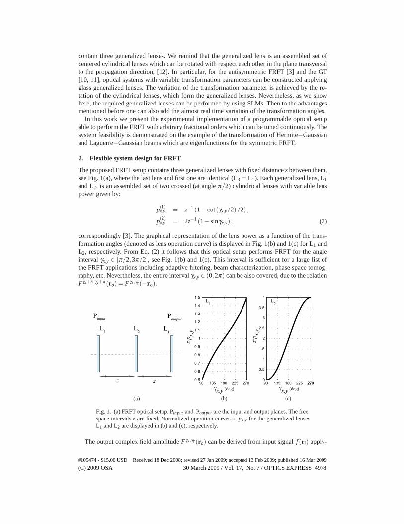
The proposed FRFT setup contains three generalized lenses with fixed distance z between them,see Fig. 1(a), where the last lens and first one are identical (L3 = L1). Each generalized lens, L1

and L2, is an assembled set of two crossed (at angle π/2) cylindrical lenses with variable lenspower given by:

p(1)x,y = z−1 (1− cot(γx,y/2)/2) ,

p(2)x,y = 2z−1 (1− sinγx,y) , (2)

correspondingly [3]. The graphical representation of the lens power as a function of the trans-formation angles (denoted as lens operation curve) is displayed in Fig. 1(b) and 1(c) for L1 andL2, respectively. From Eq. (2) it follows that this optical setup performs FRFT for the angleinterval γx,y ∈ [π/2,3π/2], see Fig. 1(b) and 1(c). This interval is sufficient for a large list ofthe FRFT applications including adaptive filtering, beam characterization, phase space tomog-raphy, etc. Nevertheless, the entire interval γx,y ∈ (0,2π) can be also covered, due to the relationFγx+π,γy+π(ro) = Fγx,γy(−ro).

z z

L1

L2

Pinput Poutput

L1

90 135 180 225 2700.5

0.6

0.7

0.8

0.9

1

1.1

1.2

1.3

1.4

1.5

90 135 180 225 2702700

0.5

1

1.5

2

2.5

3

3.5

4

(a) (b)

L1

z·px,

y

z·px,

y

γx,y (deg) γx,y (deg)

(c)

L2

Fig. 1. (a) FRFT optical setup. Pinput and Pout put are the input and output planes. The free-space intervals z are fixed. Normalized operation curves z · px,y for the generalized lensesL1 and L2 are displayed in (b) and (c), respectively.

The output complex field amplitude Fγx,γy(ro) can be derived from input signal f (ri) apply-

#105474 - $15.00 USD Received 18 Dec 2008; revised 27 Jan 2009; accepted 13 Feb 2009; published 16 Mar 2009

(C) 2009 OSA 30 March 2009 / Vol. 17, No. 7 / OPTICS EXPRESS 4978

ing the phase modulation function associated with each generalized lens L j ( j = 1,2):

Ψ j(x,y) = exp

(− iπ

λ zp( j)

x x2)

exp

(− iπ

λ zp( j)

y y2)

, (3)

and the Fresnel diffraction integral calculation, corresponding to each free-space interval. Thenthe complex field amplitude at the output plane of the FRFT setup is given by [3, 13]:

Fγx,γy(xo,yo) =1

2λ z√

sinγx sinγy

∫∫fi(xi,yi)exp

{iπ

2λ z

[(x2

o + x2i )cotγx −2xixo cscγx

]}

× exp

{iπ

2λ z

[(y2

o + y2i )cotγy −2yiyo cscγy

]}dxidyi. (4)

The latter expression coincides with the definition of the FRFT [see Eq. (1)] except for a con-stant phase factor and normalization s2 = 2λ z, which is independent of the transformationangles γx and γy. Notice that the described algorithm is used for the numerical simulation ofthis FRFT setup.

Since many applications such as beam characterization, phase retrieval, chirp detection, etc.,demand the acquisition of the FRFT squared moduli for various angles associated with inten-sity distributions, the implementation of the third generalized lens (L3 = L1) is not required.Therefore the optical setup for the measurements of the FRFT power spectra, considered be-low, consists from only two generalized lenses: L1 and L2. The rapid variation of the fractionalangles, directly related to the generalized lens powers [Eq. (2)], can be achieved by using SLMfor the lens implementation.

FRFT setup

BS

BS

SLM 2 SLM 1

SLM 3

L1

L2

z

z

Collimated laser beam

CCD

Telescope (4-f)

L L

{SLM 1

SLM 2

SLM 3

WP

WP

CCD

L

BS

BS

L

Fig. 2. Experimental setup. The amplitude and phase distributions of the input signal aregenerated by means of SLM1 (CRL-XGA2, 1024×768 pixels) and SLM2, correspond-ingly. SLM2 and SLM3 (Holoeye LCR-2500, 1024×768 pixels) implement L1 and L2lens, respectively. Output signal is registered by a CCD camera (XGA, 4.6 μm pixel size).The optical path z is set at 50 cm. SLM performance at phase-only modulation is reachedby using a λ/2 wave plate (WP).

Here we propose the experimental setup for the acquisition of the FRFT power spectra, dis-played in Fig. 2, where two reflective SLMs operating in phase-only modulation (SLM2 andSLM3) are used for lens implementation. For the input signal f (xi,yi) generation we also ap-ply a transmissive SLM (SLM1) which modulates the amplitude of a collimated Nd:YAG laserbeam with wavelength λ = 532 nm. Thus the amplitude distribution | f (xi,yi)| is implementedon SLM1 that is projected on SLM2 by using a 4-f lens system, where its phase distribution

#105474 - $15.00 USD Received 18 Dec 2008; revised 27 Jan 2009; accepted 13 Feb 2009; published 16 Mar 2009

(C) 2009 OSA 30 March 2009 / Vol. 17, No. 7 / OPTICS EXPRESS 4979

arg[ f (xi,yi)] is addressed together with the phase arg [Ψ1(x,y)] associated to the first general-ized lens. At the distance corresponding to the optical path z (in our case z = 50 cm) the SLM3is located, which implements the generalized lens L2. The intensity distribution of the outputsignal is registered by a CCD camera that is placed at the distance corresponding to the opticalpath z from the SLM3, see Fig. 2. Each SLM is connected to the same PC and the alignmentbetween them is reached digitally which is limited by the pixel size (19 μm in our case). Thusposition stages for the SLM alignment are not required. We have developed a customized soft-ware for the system control able to change the fractional orders at almost real time and to storethe measured FRFT power spectra as a video file.

3. Experimental results

In order to test the proposed experimental setup we use as input signals the Hermite−Gaussian(HG)

HGm,n (r;w) = 21/2 Hm(√

2π xw

)Hn

(√2π y

w

)

√2mm!w

√2nn!w

exp(− π

w2 r2)

, (5)

and Laguerre−Gaussian (LG)

LG±p,l (r;w) = w−1

(p!

(p+ l)!

)1/2 [√2π

( xw± i

yw

)]lLl

p

(2πw2 r2

)exp

(− π

w2 r2)

(6)

modes, where: r2 = x2 + y2, Hm is the Hermite polynomial, w is the beam waist, and Llp is the

Laguerre polynomial with radial index p and azimuthal index l. In contrast to the HG modes,the LG ones are vortex beams which carry Orbital Angular Momentum (OAM): lh̄ per photon.The HG and LG modes are eigenfunctions of the symmetric FRFT [γx = γy = γ , Ec. (4)] forw =

√2λ z (in our case w = 0.73 mm). Moreover a HG mode also does not change under the

antisymmetric FRFT (γx = −γy = γ), meanwhile a LG mode is transformed into intermediateHG−LG modes with fractional OAM: lh̄sin2γ , [14].

−1 0 1

−1

0

1

−1 0 1

−1

0

1

−1 0 1

−1

0

1

−1 0 1

−1

0

1

−1 0 1

−1

0

1

−1 0 1

−1

0

1

FRFT (0º, 0º)

y

xFRFT (0º, 0º)

y

x

FRFT (135º, 135º) FRFT (135º, -135º)

FRFT (135º, 135º) FRFT (135º, -135º)

(a) (b) (c)

(d) (e) (f)

Fig. 3. Input signals HG3,2 (a) and LG+4,1 (d) that coincide with their FRFT(0º, 0º) for each

case. Their transformations under symmetric FRFT(γ,γ) (b) (Media 1) and (e) (Media 2),as well as under antisymmetric FRFT(γ,−γ) (c) (Media 3) and (f) (Media 4) are displayed,correspondingly. The FRFT operations for angle interval γ ∈ [90º, 270º] were stored as avideo file with 30 fps. Units in axis x and y are in mm.

In particular, applying the antisymmetric FRFT for angles γ = (2k+1)π/4 to the LG±p,l (r;w)

mode, where k is an integer whereas p = min(m,n) and l = |m−n|, the HGm,n (r;w) one (ro-

#105474 - $15.00 USD Received 18 Dec 2008; revised 27 Jan 2009; accepted 13 Feb 2009; published 16 Mar 2009

(C) 2009 OSA 30 March 2009 / Vol. 17, No. 7 / OPTICS EXPRESS 4980

tated at angle ±π/4) is obtained. Therefore it is easy to test the FRFT experimental setup usingthe HG and LG modes because we know exactly their transformation for any angle. The sys-tem characterization has been done with the HG and LG modes for different indices. Here wedemonstrate the experimental results, Fig. 3, for HG3,2 3(a) and LG+

4,1 3(d) modes.The symmetric FRFT at angle γ = 135º is displayed in Fig. 3(b) and 3(e) for HG3,2 and LG+

4,1,respectively. Meanwhile the antisymmetric FRFT at angle γ = 135º is shown in Fig. 3(c) and3(f) for HG3,2 and LG+

4,1, correspondingly. These transformations have been recorded as videoat real time for the angle interval γ ∈ [90º, 270º] with step of 1º and frame rate 30 fps, seeFig. 3. As it has been expected, we observe that the intensity distributions of HG3,2 and LG+

4,1

during the transformation are almost constant except for the antisymmetric FRFT of LG+4,1

where intermediate HG−LG modes are obtained.

−1 0 1

−1

0

1

−1 0 1

−1

0

1

−1 0 1

−1

0

1

−1 0 1

−1

0

1

−1 0 1

−1

0

1

−1 0 1

−1

0

1

−1 0 1

−1

0

1

−1 0 1

−1

0

1

−1 0 1

−1

0

1

−1 0 1

−1

0

1

−1 0 1

−1

0

1

−1 0 1

−1

0

1

−1 0 1

−1

0

1

−1 0 1

−1

0

1

−1 0 1

−1

0

1

−1 0 1

−1

0

1

−1 0 1

−1

0

1

FRFT (225º, -225º) FRFT (236.3º, -236.3º) FRFT (247.6º, -247.6º) FRFT (258.9º, -258.9º)FRFT (0º, 0º) FRFT (270º, -270º)

0

0.5

1

0

π

2π

y

x

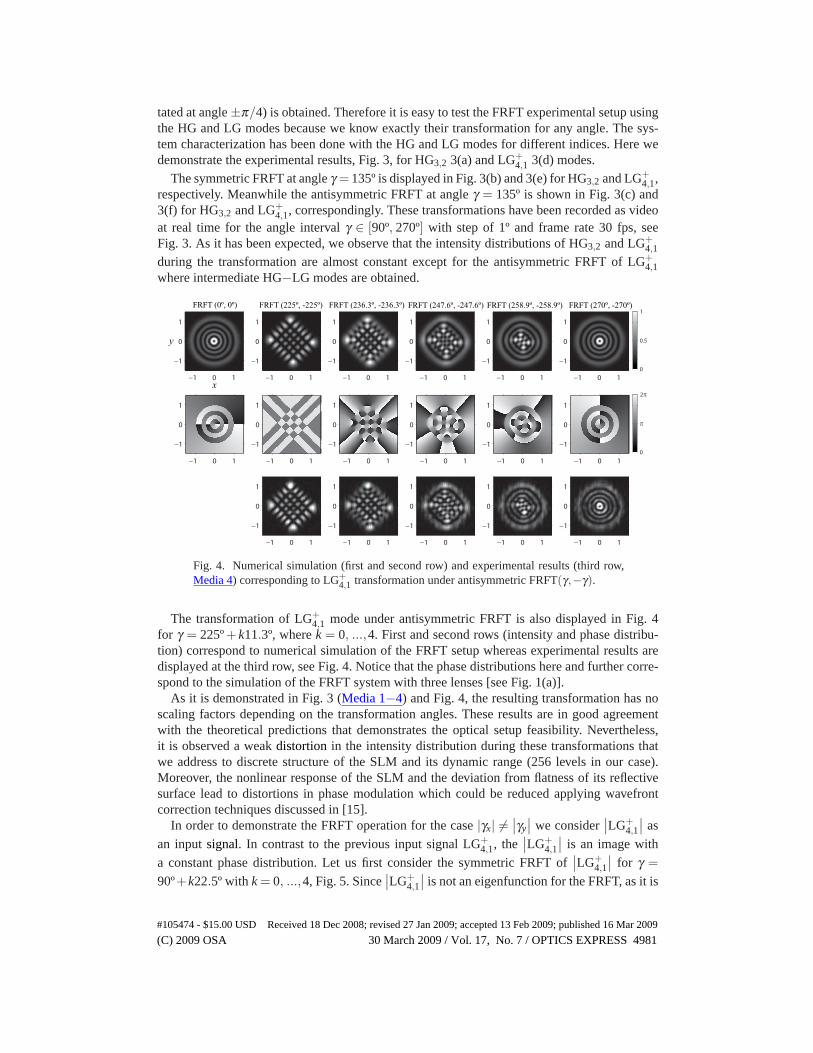
Fig. 4. Numerical simulation (first and second row) and experimental results (third row,Media 4) corresponding to LG+

4,1 transformation under antisymmetric FRFT(γ,−γ).

The transformation of LG+4,1 mode under antisymmetric FRFT is also displayed in Fig. 4

for γ = 225º + k11.3º, where k = 0, ...,4. First and second rows (intensity and phase distribu-tion) correspond to numerical simulation of the FRFT setup whereas experimental results aredisplayed at the third row, see Fig. 4. Notice that the phase distributions here and further corre-spond to the simulation of the FRFT system with three lenses [see Fig. 1(a)].

As it is demonstrated in Fig. 3 (Media 1−4) and Fig. 4, the resulting transformation has noscaling factors depending on the transformation angles. These results are in good agreementwith the theoretical predictions that demonstrates the optical setup feasibility. Nevertheless,it is observed a weak distortion in the intensity distribution during these transformations thatwe address to discrete structure of the SLM and its dynamic range (256 levels in our case).Moreover, the nonlinear response of the SLM and the deviation from flatness of its reflectivesurface lead to distortions in phase modulation which could be reduced applying wavefrontcorrection techniques discussed in [15].

In order to demonstrate the FRFT operation for the case |γx| �=∣∣γy

∣∣ we consider∣∣LG+

4,1

∣∣ as

an input signal. In contrast to the previous input signal LG+4,1, the

∣∣LG+4,1

∣∣ is an image with

a constant phase distribution. Let us first consider the symmetric FRFT of∣∣LG+

4,1

∣∣ for γ =90º+k22.5º with k = 0, ...,4, Fig. 5. Since

∣∣LG+4,1

∣∣ is not an eigenfunction for the FRFT, as it is

#105474 - $15.00 USD Received 18 Dec 2008; revised 27 Jan 2009; accepted 13 Feb 2009; published 16 Mar 2009

(C) 2009 OSA 30 March 2009 / Vol. 17, No. 7 / OPTICS EXPRESS 4981

the case for LG+4,1, the intensity distribution is changing with variation of the fractional order.

Notice that for FRFT(90º, 90º) it reduces to the Fourier transform of the input signal, whereasthe FRFT(180º, 180º) leads to self-imaging. For the rest of angles, see Fig. 5, the results aresimilar (except for scaling) to the ones obtained under Fresnel diffraction of the input signal.

−1 0 1

−1

0

1

−1 0 1

−1

0

1

−1 0 1

−1

0

1

−1 0 1

−1

0

1

−1 0 1

−1

0

1

−1 0 1

−1

0

1

−1 0 1

−1

0

1

−1 0 1

−1

0

1

−1 0 1

−1

0

1

−1 0 1

−1

0

1

−1 0 1

−1

0

1

−1 0 1

−1

0

1

−1 0 1

−1

0

1

−1 0 1

−1

0

1

−1 0 1

−1

0

1

−1 0 1

−1

0

1

−1 0 1

−1

0

1

FRFT (90º, 90º) FRFT (112.5º, 112.5º) FRFT (135º, 135º) FRFT (157.5º, 157.5º)FRFT (0º, 0º) FRFT (180º, 180º)

0

0.5

1

0

π

2π

y

x

Fig. 5. Transformation of the image∣∣LG+

4,1

∣∣ under symmetric FRFT(γ,γ). Numerical sim-

ulation (first and second row) and experimental results (third row).

−1 0 1

−1

0

1

−1 0 1

−1

0

1

−1 0 1

−1

0

1

−1 0 1

−1

0

1

−1 0 1

−1

0

1

−1 0 1

−1

0

1

−1 0 1

−1

0

1

−1 0 1

−1

0

1

−1 0 1

−1

0

1

−1 0 1

−1

0

1

−1 0 1

−1

0

1

−1 0 1

−1

0

1

−1 0 1

−1

0

1

−1 0 1

−1

0

1

0

0.5

1

0

π

2π

y

x

FRFT (90º, 135º) FRFT (135º, 180º) FRFT (180º, 225º) FRFT (225º, 270º)FRFT (0º, 0º)

Fig. 6. Transformation of∣∣LG+

4,1

∣∣ image under FRFT for γy = γx + k45º with k = 1, 2, 3.Numerical simulation (first and second row) and experimental results (third row).

Finally, we study the transformation of∣∣LG+

4,1

∣∣ under the FRFT for γy = γx + k45º withk = 1, 2 and 3, see Fig. 6. The FRFT(α, γy) and FRFT(γx, α) when α is set at 90º and 270ºcorrespond to the direct/inverse Fourier transforms along the x and y axis, respectively. It isdemonstrated in Fig. 6 for the case FRFT(90º, 135º) and FRFT(225º, 270º). For the rest of

#105474 - $15.00 USD Received 18 Dec 2008; revised 27 Jan 2009; accepted 13 Feb 2009; published 16 Mar 2009

(C) 2009 OSA 30 March 2009 / Vol. 17, No. 7 / OPTICS EXPRESS 4982

transformation angles intermediate images are obtained, Fig. 6. The comparison of the exper-imental and numerically simulated results again demonstrates the feasibility of the proposedsetup.

The fast modification of the fractional orders allows to implement various proposed algo-rithms for beam characterization, phase retrieval, information processing, etc. Moreover algo-rithms such as fractional convolution can be also implemented by using a cascade of opticalFRFT setups [1]. Since the last and first lenses corresponding to each FRFT sub-system can beaddressed into the same SLM, our setup is also able to perform such operation. Other interestingapplication is the Radon−Wigner display proposed in [16], which can be used for classifica-tion and detection of linear FM components as well as for noise reduction of one-dimensionalsignals. It contains a continuous representation of the FRFT power spectra of a signal as a func-tion of fractional order. This optical setup also involves fixed free-space intervals but it onlyperforms the one-dimensional FRFT of variable fractional orders.

4. Conclusions

Using two spatial light modulators for lens implementations we have developed an optical setupable to perform automatically the two-dimensional FRFT for an arbitrary set of fractional or-ders. The variation of the fractional parameter can be done at almost real time. In contrastto other FRFT setups, the resulting transformation has no scaling factors depending on thefractional orders. A setup characterization based on the transformation of HG and LG modeshas been demonstrated. The experimental results are in good agreement with the theoreticalpredictions and demonstrate the setup feasibility for attractive applications such as beam char-acterization, mode conversion, filtering, phase space tomography, etc.

Acknowledgments

The financial support of the Spanish Ministry of Science and Innovation under projectsTEC2005-02180, TEC2008-04105 and Santander-Complutense project PR-34/07-15914 areacknowledged. The authors thank Dr. Oscar Martínez-Matos for valuable discussions.

#105474 - $15.00 USD Received 18 Dec 2008; revised 27 Jan 2009; accepted 13 Feb 2009; published 16 Mar 2009

(C) 2009 OSA 30 March 2009 / Vol. 17, No. 7 / OPTICS EXPRESS 4983