Article

Prognosis of Water Quality Sensors Using AdvancedData Analytics: Application to the BarcelonaDrinking Water Network

Diego Garcia 1,2, Vicenç Puig 1,3,* and Joseba Quevedo 1

1 Supervision, Safety and Automatic Control Research Center (CS2AC), Universitat Politécnica de Catalunya(UPC), Terrassa Campus, Gaia Research Bldg., Rambla Sant Nebridi, 22, Terrassa, 08222 Barcelona, Spain;kobydiego@gmail.com (D.G.); joseba.quevedo@upc.edu (J.Q.)

2 Aigues de Barcelona, Empresa Metropolitana de Gestió del Cicle Integral de l’Aigua S.A.,08028 Barcelona, Spain

3 Institut de Robòtica i Informàtica Industrial (CSIC-UPC), Carrer Llorens i Artigas 4-6, 08028 Barcelona, Spain* Correspondence: vicenc.puig@upc.edu

Received: 28 December 2019; Accepted: 25 February 2020; Published: 29 February 2020

Abstract: Water Utilities (WU) are responsible for supplying water for residential, commercial andindustrial use guaranteeing the sanitary and quality standards established by different regulations. Toassure the satisfaction of such standards a set of quality sensors that monitor continuously the WaterDistribution System (WDS) are used. Unfortunately, those sensors require continuous maintenancein order to guarantee their right and reliable operation. In order to program the maintenance of thosesensors taking into account the health state of the sensor, a prognosis system should be deployed.Moreover, before proceeding with the prognosis of the sensors, the data provided with those sensorsshould be validated using data from other sensors and models. This paper provides an advanceddata analytics framework that will allow us to diagnose water quality sensor faults and to detectwater quality events. Moreover, a data-driven prognosis module will be able to assess the sensitivitydegradation of the chlorine sensors estimating the remaining useful life (RUL), taking into accountuncertainty quantification, that allows us to program the maintenance actions based on the stateof health of sensors instead on a regular basis. The fault and event detection module is based on amethodology that combines time and spatial models obtained from historical data that are integratedwith a discrete-event system and are able to distinguish between a quality event or a sensor fault. Theprognosis module analyses the quality sensor time series forecasting the degradation and thereforeproviding a predictive maintenance plan avoiding unsafe situations in the WDS.

Keywords: water quality monitoring; sensor prognosis; water distribution network

1. Introduction

The quality of the drinking water, supplied by the Water Utilities (WU) to the citizens, is regulatedby different entities to ensure full protection of public health [1]. In order to accomplish theseregulations, WU monitors the Water Distribution System (WDS) placing water quality sensors andanalyzers at different strategic locations. Moreover, experts of the WU, take samples periodically(also under regulation) at specific points of the network to analyze on-site. There are differenttypes of water quality sensors, sensors that are able to monitor a single water quality parameter ormultiple parameters.

The most common parameters monitored are temperature, chlorine, conductivity and pH. Otherparameters such as turbidity, or total organic carbon (TOC) are also measured commonly. Whichparameters to measure and how often is determined by the water quality department of the WU [2].

There are several techniques to treat the water in WDS and keep it healthy for human consumption.One common disinfection technique is the chlorination of water. This process consists of injectingchlorine or derivatives in the water. Thus, chlorine is one of the most important parameters to monitorbecause is used for disinfection purposes. The operator injects continuously a certain concentration ofchlorine in the drinking water, usually in the reservoirs, by means of an automatic controller regulatedby set-point [3]. A low concentration of chlorine can result in incomplete disinfection with consequentdanger for the citizens’ health. However, high concentrations of chlorine may produce odor andmay also increase levels of trihalomethanes (THMs) in the drinking water. Consequently, havingan accurate measure of chlorine is very important. However, it is difficult because of the injectedchlorine is consumed [4]. This consumption is related to reactions in the bulk water and in the pipewall generating a biofilm (a group of microorganisms adhered to the surface of the pipes).

A standard amperometric chlorine sensor has a membrane and electrolyte to control the reactionof the chemical reduction of hypochlorous acid at the cathode. This causes a change in the currentbetween the anode and the cathode that is proportional to the chlorine concentration. These sensorsrequire a periodic maintenance plan to clean the solids that slowly accumulate in the membraneand to replace the electrolyte. The manufacturer specifies a frequency period for each maintenanceaction required.

Another important factor to consider when measuring the chlorine is the pH dependency.The relative amount of hypochlorous acid or hypochlorite present depends on pH. Thus, to achievemore accurate chlorine measurements, the pH measurement is required.

Taking into account the complexities mentioned, this paper is focused on developing amethodology that forecasts chlorine sensor’s loss of sensitivity to keep the sensor producing reliabledata. This methodology allows the WU to increase data reliability reducing downtime and to establisha predictive maintenance plan reducing corrective actions.

Quality sensors require a continuous calibration following the procedures established by themanufacturer to produce reliable measurements. Additionally, a preventive maintenance planaccording to the manufacturer recommendations is required to guarantee data reliability.

However, even applying the recommended preventive planning, quality sensors are prone tosuffer from several problems (see Table 1). Therefore, a corrective plan is still required to address theseunexpected problems affecting the availability and reliability of the sensor.

Table 1. Problems affecting quality sensors.

Cause Consequence

Communication problem Data gapLoss of sensitivity Flat signal or slow drift down

Electronic malfunction Noise and peaksMiscalibration Offsets

On the other hand, there already exists quite a lot of research regarding methods to detect andavoid contaminant injection in the water distribution networks guaranteeing the safety of the drinkingwater network [5–7]. In [8], a comparison of a set of sensors (from different manufacturers) assessingdistinct quality parameters is carried out. This study examins the sensitivity of the different sensorsin the presence of several contaminants. In [9], the hydraulic data and water quality are consideredto minimize false positives numbers in the detection of quality events. In [10], several change-pointdetection algorithms are used to analyze the autoregressive model residual. The sensor placement ofquality sensors is also an important issue to have a good quality monitoring performance but keepinglow operational costs [11]. In [12], artificial neural networks (ANNs) are used to model the multivariatewater quality parameters and detect possible outliers. In [13], the authors explore and compare twomodels for contaminant event detection in WDS: support vector machines (SVM) and minimumvolume ellipsoid (MVE). The outputs of these two models are processed by sequence analysis to

classify the event as a normal operation or an actual quality contaminant event. In [14], incorporateshydraulic information to detect events applying spatial analysis to complement the local analysis(for each sensor) with existing mutual hydraulic influences. In [15], local and spatial data analysis isperformed using the simulation of contaminant intrusions. The proposed spatial model detects trendsin the network based on finding similar and exceptional behavior in sensors that are located upstream.In [16], spatial models considering the correlations between observations are implemented to validatewater consumption data coming from water flow sensors.

Model-based approaches, such as [7], have the main drawback that the performance dependsdirectly on the water network model’s accuracy. Moreover, due to the complex behavior of thewater parameters, it is unfeasible to develop an accurate physical model to describe the waterquality dynamics.

Hence, data-driven approaches are very interesting in this case and therefore widely used.One important drawback of data-driven approaches is the assumption that data gathered from

these sensors are accurate and precise, such as data coming from simulations. However, as we havepointed out, raw data from quality sensors could not be ready to be analyzed or to extract solidconclusions. Unreliable water quality information is a serious problem for the WU to guarantee thecitizens safety. Thus, a data cleaning process must be performed first, as [13] points out.

Hence, the main motivation of this work is to provide a data analytics methodology for monitoringquality sensors and events applicable to drinking water networks.

The contributions of this work are twofold. On the one hand, this work provides a procedure toget a solid information basis, discarding unreliable data, to improve the decision making of the WU inwater quality management. On the other hand, a prognosis module estimates the remaining useful life(RUL) of water quality sensors located in the WDS allowing the WU to apply predictive maintenance.

The proposed methodology has been satisfactorily tested on the Barcelona drinkingwater network.

The structure of the paper is the following: In Section 2, the considered case study to illustratethe proposed methodology is introduced. In Section 3, the diagnosis and prognosis methodologiesare described. In Section 4, the results obtained from three real scenarios of the considered case studyare presented and discussed. Finally, in Section 5, the conclusions are provided as well a futureresearch paths.

2. Case Study

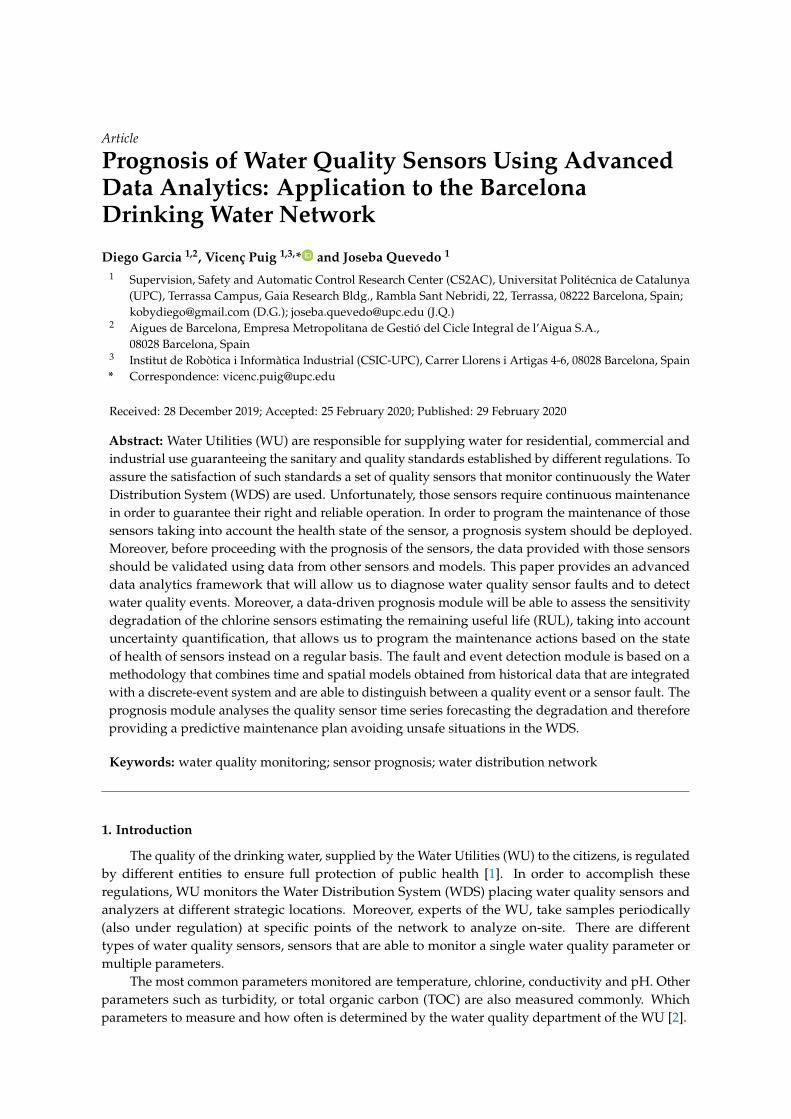
To illustrate the proposed prognosis methodology a case study based on a part of the Barcelonawater network is used. The Barcelona network is a complex water distribution system with morethan 4600 km of pipes that supply drinking water to 218 sectors of demand (see Figure 1). In thisnetwork, there are 200 quality sensors and analyzers in charge to guarantee water quality. Moreover,a laboratory sample daily several points of the network to do more in-depth analyses.

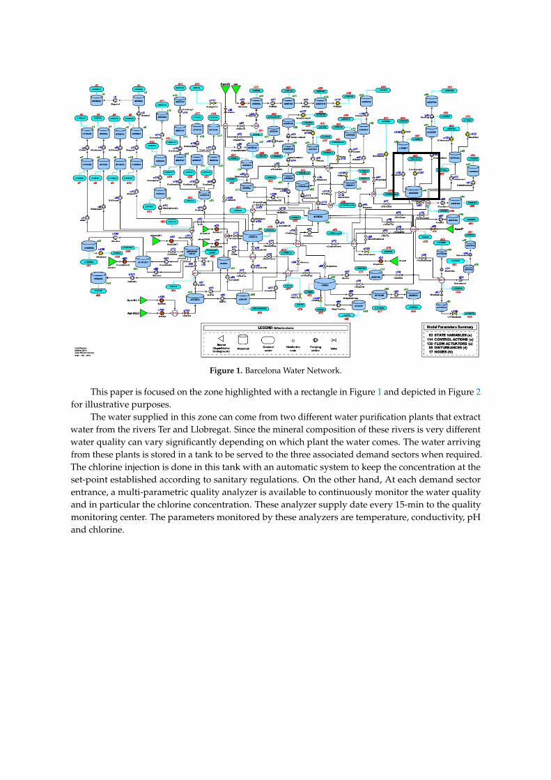
Figure 1. Barcelona Water Network.

This paper is focused on the zone highlighted with a rectangle in Figure 1 and depicted in Figure 2for illustrative purposes.

The water supplied in this zone can come from two different water purification plants that extractwater from the rivers Ter and Llobregat. Since the mineral composition of these rivers is very differentwater quality can vary significantly depending on which plant the water comes. The water arrivingfrom these plants is stored in a tank to be served to the three associated demand sectors when required.The chlorine injection is done in this tank with an automatic system to keep the concentration at theset-point established according to sanitary regulations. On the other hand, At each demand sectorentrance, a multi-parametric quality analyzer is available to continuously monitor the water qualityand in particular the chlorine concentration. These analyzer supply date every 15-min to the qualitymonitoring center. The parameters monitored by these analyzers are temperature, conductivity, pHand chlorine.

Figure 2. Case study from the Barcelona Water Network.

The water quality data collected by the sensors are analyzed by the experts using visualizationsoftware to check if there exists any quality event or problem. Then, the experts check the chlorineconcentrations measured using the sensors with the samples analyzed in the laboratory.

The methodology presented in this paper has been based on the knowledge of the experts usedto analyze. This methodology allows checking and even forecasting problems in the quality of thewater network.

3. Methodology

A diagnosis module has been designed to detect and diagnose the sensor health status. Thismodule is briefly detailed next, however, further details can be found in [17]. Moreover, a prognosismethodology has been developed to forecast the loss of sensitivity in chlorine sensors of the WDS.

3.1. Diagnosis

This module is in charge of detecting and classifying events affecting the water quality parametersby means of the analysis of local and spatial data. For each sensor, the analysis of local data is carriedusing an Artificial Neural Network (ANN) to model the behavior of the water quality time series.This model provides a prediction of the current value of the sensor based on past measurementsprovides as inputs to the ANN. This model is able to detect abrupt changes in the time series, but cannot differentiate if this change is due to fault or a quality event. These two different situations canbe distinguished by using several sensors that are spatially correlated. The predecessor (PD) spatialmodel checks the consistency between the sensor located downstream and the one located upstream.In the considered case study, the upstream sensor is the chlorine analyzer located in the tank wherethe chlorine is injected while the downstream ones are located at the entrance of the demand sectors.

Indeed, this is the procedure followed by the WU experts. First, they look for anomalous behaviorsin the signals and next they validate their conclusions looking for information from other sensorshydraulically related to conclude if it is only a sensor problem or a real water quality problem.

Following a procedure similar to those used by the human experts that analyze the qualitymeasurement, a fault diagnosis procedure is developed. This procedure works as follows: theconsistency of each local and spatial model is checked by generating a residual that is checkedagainst a threshold. The consistency check generates a 0 if the residual is below the threshold and 1

otherwise. This threshold is created by defining a lower bound τLB and upper bound τUB accordingto [18] as follows:

τLB = Q1 − 3 · IQR

τUB = Q3 + 3 · IQR(1)

where Q1 and Q3 are the first and third quartiles, respectively, and IQR is the interquartile range (thedifference between the third and first quartiles) obtained from the residuals of the training data set.

Finally, the combination of the binarized residuals are the signature of the sensor’s state accordingto the Table 2.

The fault diagnosis algorithm described above can be represented as a state machine(discrete-event system). The state diagram is presented in Figure 3. Assuming that the sensor startsin the normal (non-faulty) state, two possible situations can occur; a sensor fault or a quality event.In case a sensor fault occurs, after it is detected, the sensor fault state is reached. Finally, if the sensor isdeactivated enter the maintenance state. Finally, after the sensor is repaired, it returns to the normalstate. On the other hand, in case a quality event occurs, it can be caused by an intended action(e.g., hydraulic action, chlorine reference change) or by some unexpected infiltration.

Figure 3. State diagram of a quality sensor.

Table 2. Fault signatures of diagnosis indicators (residuals).

PD ANN PDPDPD ∧∧∧ ANN Cause

1 1 0 Sensor fault1 0 0 Sensor fault0 1 1 Quality event0 0 0 Normal state

According to Table 2, a sensor is in non-faulty situation when all residuals are within theirthresholds. On the other hand, a quality event can be identified when the ANN residual violates itsthreshold but not the PD one. Finally, when the PD residual violates its residual, a sensor fault isdiagnosed independently of the ANN residual.

3.2. Prognosis

This module forecasts the Remaining Useful Life (RUL) based on a predetermined FailureThreshold (FT). As proposed in [19], the RUL is given by:

RUL ∈ N | y(t + RUL|t) = FT, (2)

where y(t + RUL|t) is the RUL-step ahead forecast at time t of a given predictive model y.A data-driven approach is used to derive the predictive models from the data collected. Three

different methods have been considered for multi-step forecasting the chlorine decay: Brown’s doubleexponential smoothing, drift and Holt’s linear filter.

The main contribution of this module is to consider the uncertainty of the models’ estimations.In order to compute the uncertainty of each model, it is trained for a set of horizons obtaining the

optimal parameters for each forecast horizon in order to improve the models’ forecast performancewhile decreasing the residuals’ variance generated by the models.

The multi-step forecasting approach consists in fitting a model with the form

y(t + h|t, θh) (3)

where θh is the vector of parameters to adjust for each forecast horizon in 1 ≤ h ≤ H with a maximumforecast horizon H. Once a model is fitted for each horizon, a set of models are obtained for each method

Y = [y1, y2, ..., yh, ..., yH ] (4)

where yh is given by Equation (3) using a simplified notation and Y ∈ {YB, YD, YH, YNNET, YQRF, YSVM}meaning Brown, drift, holt, artificial neural networks, quantile random forests and support vectormachines methods, respectively. These methods are detailed next.

3.3. Forecast Models

The Brown’s double exponential smoothing model can be expressed as follows:

y1(t) = αhy(t) + (1− αh)y1(t− 1) (5)

y2(t) = αhy1(t) + (1− αh)y2(t− 1) (6)

a = αhh

1− αh(7)

yh(t + h|t) = (2 + a) y1(t)− (1 + a) y2(t), (8)

where h is the forecast horizon and α is the smoothing parameter.The unique parameter to be optimized for each horizon h is

θh = {α} (9)

The drift model provides a simple way to estimate the change over time from a set of observations.Indeed, it estimates the drift between the first observation and the m previous one as follows

yh(t + h|t) = y(t) + h(

y(t)− y(t−mh)

mh

), (10)

where mh is the distance between the actual observation and the previous one for a given horizon h.The set of parameters to be optimized for this model is

θh = {m} (11)

The Holt’s linear method in the state-space form is the third considered modeling approach [20].The state-space forecast general representation has the following form

y(t + h|t) = wx(t) + εh(t), (12a)

x(t) = Fx(t− 1) + ghεh(t), (12b)

where x(t) = [l(t) b(t)] is the state vector composed by the level l(t) and the growth rate b(t),

w = [1 h], F =

[1 10 1

], gh = [αh βh] and εh(t) is a random error with zero mean.

The performance of the model, as showed in [20], depends directly on the initial state x(0). In thismodel, the set of parameters to be optimized for each horizon h are

θh = {α, β, l(0), b(0)}. (13)

Multilayer Perceptron (MLP) Networks is a type of feedforward artificial neural networkconsisting of an input layer, one or multiple hidden layers, and an output layer, i.e., the modelprediction. This work considers only single-hidden-layer feed-forward neural networks (NN) withH hidden neurons. These kinds of networks are used to predict different continuous physicalprocesses [21]. Each layer is composed of one or multiple neurons and the layers are connectedone-by-one where each neuron has a direct connection to the neurons of the subsequent layer(i.e., without cycles). The basic idea of the NN construction is to adjust the corresponding weights foreach link connection between neurons minimizing an error function of the prediction using a trainingdataset. A simplification of the mathematical background of the NN expression [22] to forecast the hahead value at instant t is

yh(t + h|t) = f (x(t), wh), (14)

where x(t) = [y(t), y(t− 1), ..., y(t− N − 1)] is the vector with the N previous values of the actualtime series at time instant t and wh is the vector of the weights assigned to each neuron connection fora forecast horizon h.

Hence, the parameters to be adjusted in the NN models are

θh = {H, w} (15)

Random Forests (RF) are a powerful and popular machine learning tool for high dimensionalclassification and regression [23]. RF are a combination of tree predictors that vote for the most popularclass for classification or provide the average of the trees predictors for regression. Given an input x,a tree predictor T(x, Θ) provides a categorical value (classification) or a continuous value (regression).Basically, the prediction trees sub-divide the complex input space into smaller partitions, recursively,in order to obtain small cells where a simple model or even a constant value (the average) can representthe cell group. It starts at a root and the final cells are the leaves. How to split and which features areinvolved in each split is part of the training phase. The structure of the tree is represented by Θ.

Quantile Regression Forest (QRF) is a generalization of RF, as it provides not only the conditionalmean, but also estimates the conditional quantiles [24]. The RF final prediction (in the regression form)for a given new input x is made averaging the predictions from all the B individual regression trees

yh(t + h|t) = 1Bh

Bh

∑b=1

T(x(t); Θbh), (16)

where is the individual tree regression function and Θbh characterizes the b-th random forest tree fora given forecast horizon h. The input vector x(t) = [y(t), y(t− 1), ..., y(t− N − 1)] is the vector withthe N previous values of the actual time series at time instant t, and Bh is the number of randomforest trees.

Hence, the QRF parameters to be tuned are

θh = {B, Θb} (17)

RF have been implemented using the R package rpart [25].

The goal of Support Vector Machines (SVM) is to find a function f (x) given a training dataset{(x1, y1), ..., (xm, ym)} ⊂ X ×R where X is the space of the input predictors and yi the target. In caseof a linear function f , it takes the form

f (x) = 〈w, x〉+ b, (18)

where w ∈ X , b ∈ R and 〈· , · 〉 denotes the scalar product inX . For nonlinear functions, the input spaceis mapped first into a new feature space F using a mapping function Φ : X → F [26]. The forecastexpression of SVM is

y(t + h|t) =Lh

∑i=1

(αih − α∗ih)k(xi(t), x(t)) + bh, (19)

where αi and α∗i are Lagrange multipliers and k(xi(t), x(t)) is the mapping function, known as thekernel function, x(t) = [y(t), y(t− 1), ..., y(t− N − 1)] is the vector of the N previous values of theactual time series and xi(t) is the element i of the input vector, i.e., y(t− i + 1).

Hence, the parameters to be adjusted in the SVM models are

θh = {L, αi, α∗i , b} (20)

3.4. Models Performance Metric

Two different metrics are used to assess the model’s performance. On the one hand, for thelinear models, the training stage finds the optimum parameter values for each model minimizing, as afunction cost, the mean absolute percentage error (MAPE) defined as

min1n

n

∑t=1

∣∣∣y(t + h)− y(t + h|t, θh)

y(t + h)

∣∣∣, (21)

where θh is the vector of parameters for all 1 ≤ h ≤ H of each linear model to be optimized accordingto Equations (9), (11) and (13), respectively.

On the other hand, for the nonlinear models, the training stage finds the optimum parametervalues for each model minimizing the root mean square (RMSE) defined as

min

√1n

n

∑t=1

[y(t + h)− y(t + h|t, θh)]2 (22)

where θh is the vector of parameters for all 1 ≤ h ≤ H of each nonlinear model to be optimizedaccording to Equations (15), (17) and (20), respectively.

Moreover, the training of nonlinear models is performed with k-fold cross-validation to avoidthe over-fitting of the models. K-cross-validation splits the dataset randomly into k equal subsamples.One of these k subsamples is used for validation and testing and the rest is used for training the model.The cross-validation is then repeated k times using each sample only once.

3.5. Prognosis Performance Evaluation

In order to evaluate the prognosis models performance, the Prognosis Horizon (PH) iscomputed as

PH = tFT − i, (23)

where tFT is the time instant of FT (see Equation (2)), and i is expressed as

argmini|tFT − (j + RULj)| ≤ ε, ∀j ∈ [i, tFT] (24)

and ε is the admissible error bound.

4. Results

In this section, results based on the Barcelona case study, detailed in Section 2, are presented nextto show the performance of the methodology proposed in this work.

The methodology presented has been tested off-line using real data from several past scenarios [27].This work addresses the methodology that will be used on-line by the WU in a medium-term future,once the on-line requirements have been validated and analyzed.

The results presented here are focused on the prognosis module. The diagnosis module resultsare already presented in [17], showing anticipation of the sensor fault detection in about 12 daysbefore the experts reported the sensor incidences. Thus, the data used by the prognosis module,to generate the results presented in this section, have been previously validated and processed by thediagnosis module.

The data used to generate the results come from the multi-parametric (chlorine, pH, temperatureand conductivity) sensors (0794, 0795 and 0801), the chlorine analyzer X127701D and the incidencesreported by the WU experts to the maintenance department (applied to the part of the Barcelonanetwork presented in Figure 2).

The chlorine concentration observed is around 0.5 mg/L and the minimum value allowed bythe Government of Catalonia regulation of chlorine concentration in the WDS is 0.2 mg/L. Hence,the minimum threshold to train the models is FT = 0.2.

The scenarios analyzed are three different chlorine decay scenarios. Figure 4 shows the threescenarios A, B and C, vertically stacked. The long-dashed blue line is the chlorine signal of VX127701D,the transport analyzer placed in the reservoir (see Figure 2). The dashed green line is the V0795 chlorinesignal. The solid red line is the V0794 chlorine signal. As it can be noted, the chlorine decays are notequal in velocity and linearity. Scenario A shows a slow decay till 0.2 of chlorine in tFT = 378 h (16days) with some slumps. Scenario B shows a decay to 0.2 of chlorine in tFT = 147 h (6 days). ScenarioC shows a chlorine decay in tFT = 130 h (5 days). Scenario B presents the most linear decay of them.While scenario C presents a slight curve at the end. As it will show next, these factors (slumps andnon-linear decays) impacts directly on the prognosis performance.

0.2

0.3

0.4

0.5

0.6

0.7

0.2

0.3

0.4

0.5

0.6

0.7

0.2

0.3

0.4

0.5

0.6

0.7

Sce

na

rio A

S

ce

na

rio B

Sce

na

rio C

0 100 200 300 400

time index (hours)

Ch

lori

ne

tag V0794 V0795 VX127701D

Figure 4. Fault scenarios of chlorine sensors.

The prognosis performance metric PH, Equation (23), have been evaluated on the six modelsdetailed in Section 3 with ε = 0.10× H and H = 90, i.e., ε = 9. As mentioned before, the modelsare trained using one scenario and evaluated with the others to avoid over-fitting and evaluate thegeneralization. Figure 5 shows the PH evaluation training each model with one scenario (stacked

vertically) and tested with the others (stacked horizontally). The bar plots in the diagonal are theevaluation of the training data sets.

5

49

88

17

90

9

1325

145 5 5

5 6 10 6 5 5

2740

121 2 6

36

16

60

7

90 90

27 2311

2413

49

18 14 120 0 5

16 14 12 7

54

14

20 14

58

24

90 89

Scenario A Scenario B Scenario C

Scenario

AS

cenario

BS

cenario

C

Bro

wn

Dri

ft

ET

S

NN

ET

QR

F

SV

M

Bro

wn

Dri

ft

ET

S

NN

ET

QR

F

SV

M

Bro

wn

Dri

ft

ET

S

NN

ET

QR

F

SV

M

0

30

60

90

0

30

60

90

0

30

60

90

Method

PH

(h

ou

rs)

Test scenario

Train

scen

ario

Figure 5. Evaluation of the prognosis performance using the PH metric.

Finally, to summarize the performance results, Figure 6 shows the PH average for each testingscenario, and again leaving out the scenarios where training and testing are both the same in order toevaluate the generalization performance.

0

5

10

15

20

25

30

35

Scenario A Scenario B Scenario C

Test scenario

ave

rage P

H (

hours

)

method

Brown

Drift

ETS

NNET

QRF

SVM

Figure 6. Average PH leaving out the scenarios that are the same for training and testing.

As can be noted, ETS, QRF and SVM algorithms show a good performance when the training andtesting scenarios are both the same (see the diagonal results in Figure 5). However, the PH averagein Figure 6, shows clearly the poor performance of ETS, NN and QRF methods when are applied totesting scenarios different than training scenarios, excluding QRF applied to scenario C. In contrast,drift and Brown methods have the best performance with highest PH averages in Figure 6. Onerelevant fact that can be observed in Figure 6 is the higher average performance obtained in scenario Bby almost any model compared against in scenarios A and C. This is because the decay of scenario B ismore linear than in A and C (see Figure 4) and therefore more predictable.

The bad performance of the models NN and QRF is due to the model construction process. Thesekinds of machine learning models require a lot of data, i.e., a large set of scenarios, to train them inorder to generalize properly with new unseen scenarios. In this work, these models have been trainedwith only one scenario and tested with the others, therefore obtaining worst performance than Brown

and drift models. With the exception of the SVM model, which uses only one scenario for training,and is able to perform similar to the Brown model.

The results of the first row of bar plots from Figure 5 are discussed below. Figures from 7 to 18present the results obtained with the different results models trained with scenario A and applied tothe scenarios B and C.

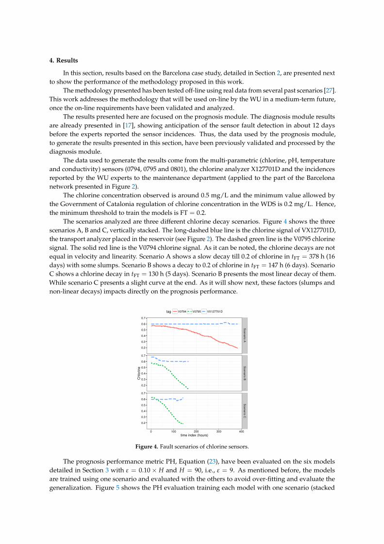
Figures 7–9 show the drift, Brown and SVM results when trained with scenario A and applied toscenario B. As commented before, this good performance is due to the linearity of the chlorine decayat the end of scenario B. In contrast, scenario A has small bumps at the end and scenario C has a slightcurve leading to worse performances. Figures 10–12 show the inferior performance on scenario C bythe drift, Brown and SVM models, respectively.

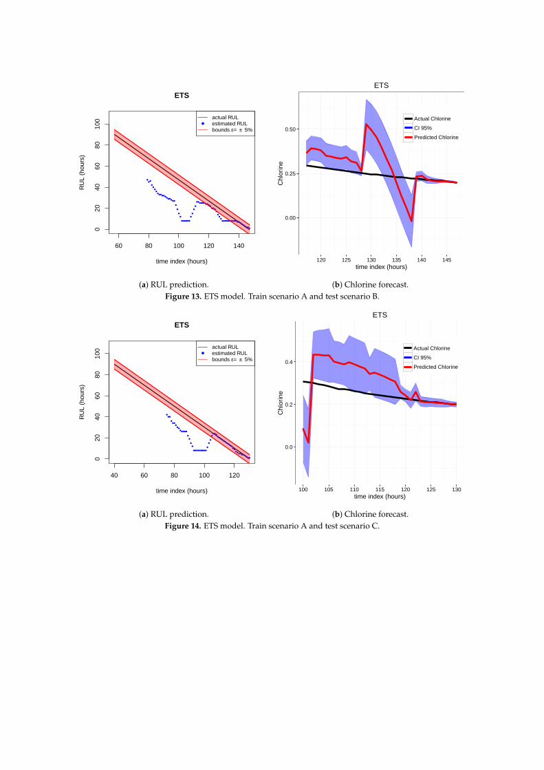
As indicated before, ETS (Figures 13 and 14), NN (Figures 15 and 16) and QRF (Figures 17 and 18)show a poor generalization.

60 80 100 120 140

020

4060

8010

0

Drift

time index (hours)

RU

L (h

ours

)

●

●●

●

●

●

●

●●

●●

●●

●●

●●

●●

●●

●●

●●

●●

●●●

●●

●●

●●

●●●

●●

●●

●●●

●●●●

●●●

●●

●●●

●

●

actual RULestimated RULbounds ε= ± 5%

(a) Remaining useful life (RUL) prediction.

0.20

0.25

0.30

0.35

120 125 130 135 140 145time index (hours)

Chl

orin

eActual Chlorine

CI 95%

Predicted Chlorine

Drift

(b) Chlorine forecast.Figure 7. Drift model. Train scenario A and test scenario B.

60 80 100 120 140

020

4060

8010

0

Double exponential smoothing

time index (hours)

RU

L (h

ours

)

●

●●

●

●

●●

●

●●

●●

●●

●●

●●

●●

●●

●●

●●

●●

●●

●

●

●

●

●●

●●

●●

●●

●●●

●●●

●●●

●●●

●●●

●●

●

actual RULestimated RULbounds ε= ± 5%

(a) RUL forecast.

0.2

0.3

0.4

0.5

120 125 130 135 140 145time index (hours)

Chl

orin

e

Actual Chlorine

CI 95%

Predicted Chlorine

Double exponential smoothing

(b) Chlorine forecast.Figure 8. Brown model. Train scenario A and test scenario B.

60 80 100 120 140

020

4060

8010

0svmPoly

time index (hours)

RU

L (h

ours

) ●●●

●●

●●●●

●

●

●

●

●

●

●

●

●

●●

●●

●●●

●●

●●

●●

●●

●

●

actual RULestimated RULbounds ε= ± 5%

(a) RUL prediction.

0.2

0.3

0.4

0.5

0.6

120 125 130 135 140 145

time index (hours)

Chl

orin

e

Actual Chlorine

CI 95%

Predicted Chlorine

svmPoly

(b) Chlorine forecast.Figure 9. SVM model. Train scenario A and test scenario B.

40 60 80 100 120

020

4060

8010

0

Drift

time index (hours)

RU

L (h

ours

)

●●

●

●●

●●

●

●

●

●●

●●

●●

●●

●●

●●

●●

●●

●●

●●

●●

●●

●●

●●

●●

●●

●●

●●

●●●●

●●●●

●●●

●●

●●●

●●●

●

actual RULestimated RULbounds ε= ± 5%

(a) RUL prediction.

0.20

0.25

0.30

0.35

100 105 110 115 120 125 130time index (hours)

Chl

orin

e

Actual Chlorine

CI 95%

Predicted Chlorine

Drift

(b) Chlorine forecast.Figure 10. Drift model. Train scenario A and test scenario C.

40 60 80 100 120

020

4060

8010

0Double exponential smoothing

time index (hours)

RU

L (h

ours

)

●●

●●

●●

●●

●●

●

●●

●●

●●

●●

●●

●●

●●

●●

●●

●●

●

●

●

●

●

●●●

●●

●●

●●●

●●●

●●●●

●●●

●●

●●●

●●●

●

actual RULestimated RULbounds ε= ± 5%

(a) RUL forecast.

0.2

0.3

0.4

0.5

100 105 110 115 120 125 130time index (hours)

Chl

orin

e

Actual Chlorine

CI 95%

Predicted Chlorine

Double exponential smoothing

(b) Chlorine forecast.Figure 11. Brown model. Train scenario A and test scenario C.

40 60 80 100 120

020

4060

8010

0

svmPoly

time index (hours)

RU

L (h

ours

)

●●

●●

●●●

●●

●

●

●

●

●

●

●

●●

●●

●●

●●

●●

●●

●●

●

actual RULestimated RULbounds ε= ± 5%

(a) RUL prediction.

0.3

0.5

0.7

0.9

100 105 110 115 120 125 130

time index (hours)

Chl

orin

e

Actual Chlorine

CI 95%

Predicted Chlorine

svmPoly

(b) Chlorine forecast.Figure 12. SVM model. Train scenario A and test scenario C.

60 80 100 120 140

020

4060

8010

0ETS

time index (hours)

RU

L (h

ours

)

●●

●

●●

●●

●●●

●●●

●●●

●●●

●

●

●

●

●●●●●●

●

●

●

●

●●●●●●

●●●

●●●

●●

●●

●●●●●●●●●●●

●●●

●●

●●●

●

●

actual RULestimated RULbounds ε= ± 5%

(a) RUL prediction.

0.00

0.25

0.50

120 125 130 135 140 145time index (hours)

Chl

orin

e

Actual Chlorine

CI 95%

Predicted Chlorine

ETS

(b) Chlorine forecast.Figure 13. ETS model. Train scenario A and test scenario B.

40 60 80 100 120

020

4060

8010

0

ETS

time index (hours)

RU

L (h

ours

)

●●●

●●●

●●

●●

●●●●

●

●

●

●

●●●●●●●●●

●

●

●

●●●

●●

●●

●●

●●

●●

●●

●●

●●●

●●●

●●●

●

actual RULestimated RULbounds ε= ± 5%

(a) RUL prediction.

0.0

0.2

0.4

100 105 110 115 120 125 130time index (hours)

Chl

orin

e

Actual Chlorine

CI 95%

Predicted Chlorine

ETS

(b) Chlorine forecast.Figure 14. ETS model. Train scenario A and test scenario C.

60 80 100 120 140

020

4060

8010

0nnet

time index (hours)

RU

L (h

ours

)

●●●●●

●●

●

●

●

●●

●●

●●

●●

●●

●●●

●●

●●

●●

●

●

●

●

●

●

●

●

●●

●

actual RULestimated RULbounds ε= ± 5%

(a) RUL prediction.

0.2

0.3

0.4

0.5

0.6

0.7

120 125 130 135 140 145

time index (hours)

Chl

orin

e

Actual Chlorine

CI 95%

Predicted Chlorine

nnet

(b) Chlorine forecast.Figure 15. NN model. Train scenario A and test scenario B.

40 60 80 100 120

020

4060

8010

0

nnet

time index (hours)

RU

L (h

ours

)

●●●●●●●

●

●

●

●

●●

●●

●

●●

●●●

●●

●●

●●

●

●

●

●

●

●

●

●

●

actual RULestimated RULbounds ε= ± 5%

(a) RUL prediction.

0.25

0.50

0.75

1.00

100 105 110 115 120 125 130

time index (hours)

Chl

orin

e

Actual Chlorine

CI 95%

Predicted Chlorine

nnet

(b) Chlorine forecast.Figure 16. NN model. Train scenario A and test scenario C.

60 80 100 120 140

020

4060

8010

0qrf

time index (hours)

RU

L (h

ours

)

●●

●●

●●

●●

●

●

●

●●

●●

●●

●

●

●

●

●●

●●

●●

●

●●

●●

●●

●●

●

●

actual RULestimated RULbounds ε= ± 5%

(a) RUL prediction.

0.2

0.3

0.4

0.5

0.6

120 125 130 135 140 145

time index (hours)

Chl

orin

e

Actual Chlorine

CI 95%

Predicted Chlorine

qrf

(b) Chlorine forecast.Figure 17. QRF model. Train scenario A and test scenario B.

40 60 80 100 120

020

4060

8010

0

qrf

time index (hours)

RU

L (h

ours

)

●

●●

●●

●

●

●

●●

●●

●●

●

●

●

●

●

●●

●●

●●

●●

●●

●

●

●

actual RULestimated RULbounds ε= ± 5%

(a) RUL prediction.

0.2

0.4

0.6

100 105 110 115 120 125 130

time index (hours)

Chl

orin

e

Actual Chlorine

CI 95%

Predicted Chlorine

qrf

(b) Chlorine forecast.Figure 18. QRF model. Train scenario A and test scenario C.

5. Conclusions

This paper presents a prognosis approach for the water quality sensors using advanced dataanalytics approaches.

The complexity of chlorine sensors requires a regular maintenance plan to avoid monitorunreliable data and infer wrong conclusions. The prognosis framework presented can help theWU to predict these faulty states in order to apply predictive maintenance. Therefore, this allowsdecreasing corrective actions reducing OPEX costs of the WU.

On the one hand, a diagnosis framework has been briefly discussed that guarantees that no eventor sensor fault is present before running the prognosis approach [17]. On the other hand, a prognosisframework has been presented to predict the RUL of chlorine sensors that presents a chlorine decaydue to loss of sensitivity. The proposed prognosis approach has been assessed using three real scenariosfrom the Barcelona Water Network.

Brown and drift methods have shown a bad performance when non-linear shapes are present onthe chlorine decay, such as bumps and curves. While the ETS method shows poor performance whenapplied to different scenarios that the trained one indicating an inherent over-fitting behavior. The driftmethod shows the best performance average, but Brown showing a slightly less performance averagehas less variance. For this reason, Brown is the one proposed to be used in the real implementation.

In contrast, the nonlinear models considered (NNET, QRF and SVM) do not provide the expectedgood results due to the reduced amount of data used for model construction. They require a largernumber of training scenarios to generalize properly with new unseen scenarios.

The complexity of the model is an important requirement for the experts of the WU. Therefore,according to the performance and the simplicity of the implementation, the Brown method is theoptimal choice for the prognosis module, discarding the other methods.

The methodology and the results detailed in this work have been presented to the experts of theWU. They expressed their approval and satisfaction with the results obtained. However, this work is astudy phase of the methodology and it is not implemented on-line by the WU yet.

Finally, future work will deal with the on-line deployment of the proposed methodology.Moreover, many more decay scenarios in order to improve the machine learning model’s performancewill be considered.

Author Contributions: Conceptualization, V.P. and J.Q.; methodology, all; software, D.G.; validation, D.G.;writing–original draft preparation, all; writing–review and editing, all. All authors have read and agreed to thepublished version of the manuscript.

Funding: This work has been funded by SMART Project (ref. num. EFA153/16 Interreg Cooperation ProgramPOCTEFA 2014-2020)

Conflicts of Interest: The authors declare no conflict of interest.

References

1. Guidelines for Drinking Water Quality, 4th ed.; World Health Organization: Geneva, Switzerland, 2004.2. Bartram, J.; Ballance, R. Water Quality Monitoring: A Practical Guide to the Design and Implementation of

Freshwater Quality Studies and Monitoring Programs; E & FN Spon: London, UK, 1996.3. Karadirek, I.; Kara, S.; Muhammetoglu, A.; Muhammetoglu, H.; Soyupak, S. Management of chlorine

dosing rates in urban water distribution networks using online continuous monitoring and modeling.Urban Water J. 2016, 13, 345–359. [CrossRef]

4. Powell, J.C.; Hallam, N.B.; West, J.R.; Forster, C.F.; Simms, J. Factors which control bulk chlorine decayrates. Water Res. 2000, 34, 117–126. [CrossRef]

5. Byer, D.; Carlson, K.H. Expanded Summary: Real-time detection of intentional chemical contamination inthe distribution system. J. Am. Water Work. Assoc. 2005, 97, 130–133. [CrossRef]

6. Hou, D.; Liu, S.; Zhang, J.; Chen, F.; Huang, P.; Zhang, G. Online Monitoring of Water-Quality Anomaly inWater Distribution Systems Based on Probabilistic Principal Component Analysis by UV-Vis AbsorptionSpectroscopy. J. Spectrosc. 2014, 2014. [CrossRef]

7. Eliades, D.; Lambrou, T.; Panayiotou, C.; Polycarpou, M. Contamination Event Detection in WaterDistribution Systems Using a Model-based Approach. Procedia Eng. 2014, 89, 1089–1096. [CrossRef]

8. Hall, J.; Zaffiro, A.D.; Marx, R.B.; Kefauver, P.C.; Krishnan, E.R.; Haught, R.C.; Herrmann, J.G. On-LineWater Quality Parameters as Indicators of Distribution System Contamination. J. - Am. Water Work. Assoc.2007, 99, 66–77. [CrossRef]

9. Hart, D.B.; McKenna, S.a.; Murray, R.; Haxton, T. Combining Water Quality and Operational Data forImproved Event Detection. In Proceedings of the 12th Annual Conference on Water Distribution SystemsAnalysis (WDSA), Tucson, AZ, USA, 12–15 September 2010; pp. 287–295. doi:10.1061/41203(425)26.[CrossRef]

10. Ba, A.; McKenna, S.A. Water quality monitoring with online change-point detection methods. J.Hydroinformatics 2015, 17, 7. [CrossRef]

11. Rathi, S.; Gupta, R. Sensor Placement Methods for Contamination Detection in Water DistributionNetworks: A Review. Procedia Eng. 2014, 89, 181–188. [CrossRef]

12. Perelman, L.; Arad, J.; Housh, M.; Ostfeld, A. Event detection in water distribution systems frommultivariate water quality time series. Environ. Sci. Technol. 2012, 46, 8212–9. [CrossRef] [PubMed]

13. Oliker, N.; Ostfeld, A. Comparison of two multivariate classification models for contamination eventdetection in water quality time series. J. Water Supply: Res. -Technol. 2015, 64, 558. [CrossRef]

14. Oliker, N.; Ostfeld, A. Network hydraulics inclusion in water quality event detection using multiple sensorstations data. Water Res. 2015, 80, 47–58. [CrossRef] [PubMed]

15. Oliker, N.; Ohar, Z.; Ostfeld, A. Spatial event classification using simulated water quality data. Environ.Model. Softw. 2016, 77, 71–80. [CrossRef]

16. Quevedo, J.; Alippi, C. Temporal/spatial model-based fault diagnosis vs. Hidden Markov models changedetection method: Application to the Barcelona water network. In Proceedings of the 21st MediterraneanConference on Control and Automation, Chania, Greece, 25–28 June 2013.

17. García, D.; Creus, R.; Minoves, M.; Pardo, X.; Quevedo, J.; Puig, V. Data analytics methodology formonitoring quality sensors and events in the Barcelona drinking water network. J. Hydroinform. 2016,doi:10.2166/hydro.2016.048. [CrossRef]

18. Tukey, J.W. Addison-Wesley Series in Behavioral Science: Quantitative Methods. In Exploratory DataAnalysis; Addison-Wesley: Boston, MA, USA, 1977.

19. Escobet, T.; Quevedo, J.; Puig, V. A Fault / Anomaly System Prognosis using a Data- driven Approachconsidering Uncertainty. In Proceedings of the 2012 International Joint Conference on Neural Networks(IJCNN), Brisbane, QLD, Australia, 10–15 June 2012; pp. 10–15. [CrossRef]

20. Hyndman, R.; Koehler, A.; Snyder, R.; Grose, S. A state space framework for automatic forecasting usingexponential smoothing methods. Int. J. Forecast. 2002, 18, 439–454. [CrossRef]

21. Sun, A.Y. Predicting groundwater level changes using GRACE data. Water Resour. Res. 2013, 49, 5900–5912.[CrossRef]

22. Svozil, D.; Kvasnicka, V.; Pospichal, J. Introduction to multi-layer feed-forward neural networks. Chemom.Intell. Lab. Syst. 1997, 39, 43 – 62. [CrossRef]

23. Breiman, L. Random forests. Mach. Learn. 2001, 45, 5–32, doi:10.1023/A:1010933404324. [CrossRef]24. Meinshausen, N. Quantile Regression Forests. J. Mach. Learn. Res. 2006, 7, 983–999. [CrossRef]25. Therneau, T.; Atkinson, B.; Ripley, B. rpart: Recursive Partitioning and Regression Trees. 2015. R

Package Version 4.1-10. Available online: https://r.789695.n4.nabble.com/attachment/3209029/0/zed.pdf(accessed on 28 December 2019).

26. Smola, A.J.; Schölkopf, B. A tutorial on support vector regression. Stat. Comput. 2004, 14, 199–222.[CrossRef]

27. García, D.; Creus, R.; Minoves, M.; Pardo, X.; Quevedo, J.; Puig, V. Prognosis of quality sensors inthe Barcelona drinking water network. In Proceedings of the 2016 3rd Conference on Control andFault-Tolerant Systems (SysTol), Barcelona, Spain, 7–9 September 2016; pp. 446–451.