Prof. Aiken CS 294 Lecture 41 Constraint-Based Analysis Lecture 4.
68
Prof. Aiken CS 294 Lecture 4 1 Constraint-Based Analysis Lecture 4
-
date post
20-Dec-2015 -
Category
Documents
-
view
213 -
download
0
Transcript of Prof. Aiken CS 294 Lecture 41 Constraint-Based Analysis Lecture 4.

Prof. Aiken CS 294 Lecture 4 1
Constraint-Based Analysis
Lecture 4

Prof. Aiken CS 294 Lecture 4 2
Outline
• Review– Dataflow– Type inference
• A generalization: Set constraints– Intractable/tractable problems – Solving constraints
• Examples• Optimizations• Summary

Prof. Aiken CS 294 Lecture 4 3
Dataflow Problems
• Classical dataflow equations are described as:
• v is a variable, a is an atom• System of inclusion constraints• Only variables on lhs• Domain is atoms
( )
| | |i i iv E
E E E E E v a

Prof. Aiken CS 294 Lecture 4 4
Type Inference Problems
• Type inference problems are described as:
Æi i1 = i2
= c(, . . ., ) |
• c is a constructor (may be 0-ary)• System of equations• Arbitrary expressions on lhs and rhs• Domain is terms

Prof. Aiken CS 294 Lecture 4 5
Summary
• Dataflow analysis– Inclusion constraints over atoms
• Type inference– Equations over terms
• Two very different theories– With different applications– Developed over decades
• But are they really independent?

Prof. Aiken CS 294 Lecture 4 6
Set Constraints
• The set expressions are:E ::= 0 | | E [ E | E Å E | :E | c(E,…,E) | ci
-1(E)
• A system of set constraints is Æi Ei1 µ Ei2
• Constructors c• Set variables

Prof. Aiken CS 294 Lecture 4 7
Semantics of Set Expressions
E ::= 0 | | E [ E | E Å E | :E | c(E,…,E) | ci-1(E)
• One interpretation: Set expressions denote subsets of the Herbrand Universe H
• An assignment maps variables to sets of terms:
: Vars ! 2H

Prof. Aiken CS 294 Lecture 4 8
Semantics of Set Expressions (Cont.)
E ::= 0 | | E [ E | E Å E | :E | c(E,…,E) | ci-1(E)
• Extend to all set expressions: (0) = ;
(E1 [ E2) = (E1) [ (E2)
(E1 Å E2) = (E1) Å (E2)
(:E) = H - (E) (c(E1,…,En)) = {c(t1,…,tn) | ti 2 (Ei)}
(ci-1(E)) = { ti | c(t1,…,tn) 2 (E) }

Prof. Aiken CS 294 Lecture 4 9
Solutions
• An assignment is a solution of the constraints if
Æi (Ei1) µ (Ei2)

Prof. Aiken CS 294 Lecture 4 10
Set Constraints
• Set constraints generalize– Dataflow equations (add terms)– Type equations (add inclusion constraints)– And more (add projections)
Dataflow Equations
Type Equations
Set Constraints

Prof. Aiken CS 294 Lecture 4 11
Notes on Projection
• Projection can model data selectors– Car, cdr, hd, tl, etc.
• But projections have another interesting property:
1 if 0( ( , ))
0 otherwise
A Bc c A B

Prof. Aiken CS 294 Lecture 4 12
Conditional
• Projections can be used to encode conditional constraints:
B 0 ) A µ C ´ c-1(c(A,B)) µ C

Prof. Aiken CS 294 Lecture 4 13
Complexity
Thm Deciding whether a system of set constraints has any solutions is NEXPTIME-complete
• Remains NEXPTIME complete even if we drop projections
• So, focus on tractable sub-theories
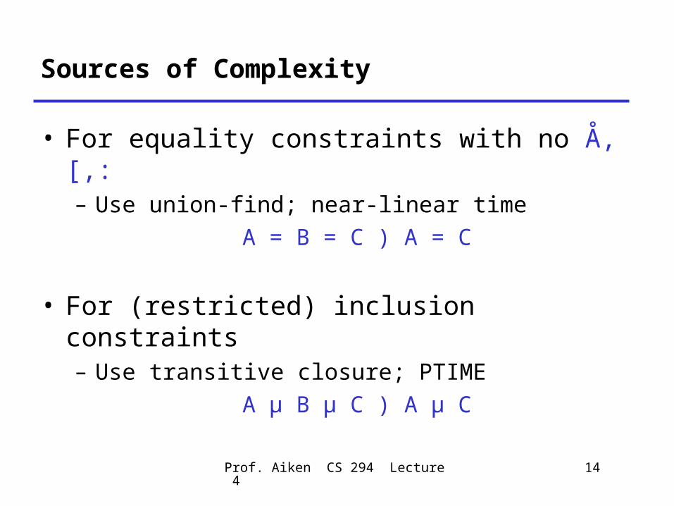
Prof. Aiken CS 294 Lecture 4 14
Sources of Complexity
• For equality constraints with no Å,[,:– Use union-find; near-linear time
A = B = C ) A = C
• For (restricted) inclusion constraints– Use transitive closure; PTIME
A µ B µ C ) A µ C

Prof. Aiken CS 294 Lecture 4 15
Sources of Complexity (Cont.)
• For EXPTIME algorithms, general Å,[,:
• For NEXPTIME algorithms, the choiceC(A, B) = 0 , A = 0 Ç B = 0

Prof. Aiken CS 294 Lecture 4 16
Connections
• Set constraints are related to– Tree automata– Logic (the monadic class)
• Also, implementation techniques are based on graphs & graph algorithms

Prof. Aiken CS 294 Lecture 4 17
A Tractable Fragment
L ::= L [ L | c(L,…,L) | | 0R ::= R Å R | c(R,…,R) | | 1
Let C be constraints of the form:L µ R
0 ) L µ R

Prof. Aiken CS 294 Lecture 4 18
Solving Set Constraints
• The usual strategy:– Rewrite constraints, preserving solutions– When all possible rewrites have been done, the
system is in “solved form”• Solutions are manifest
• Note: there are different notions of “solve”– Has at least one solution (yes/no)– Describe one solution (e.g., the least)– Describe all solutions

Prof. Aiken CS 294 Lecture 4 19
Resolution Rules 1
• Trivial constraints:S Æ L µ 1 , SS Æ 0 µ R , SS Æ x µ x , S

Prof. Aiken CS 294 Lecture 4 20
Resolution Rules 2
More interesting constraints:
Lµ R1 Å R2 , L µ R1 Æ L µ R2
L1 [ L2 µ R , L1 µ R Æ L2 µ R
c(…) µ Æ µ R , c(…) µ Æ µ R Æ c(…) µ R
Prof. Aiken CS 294 Lecture 4 21
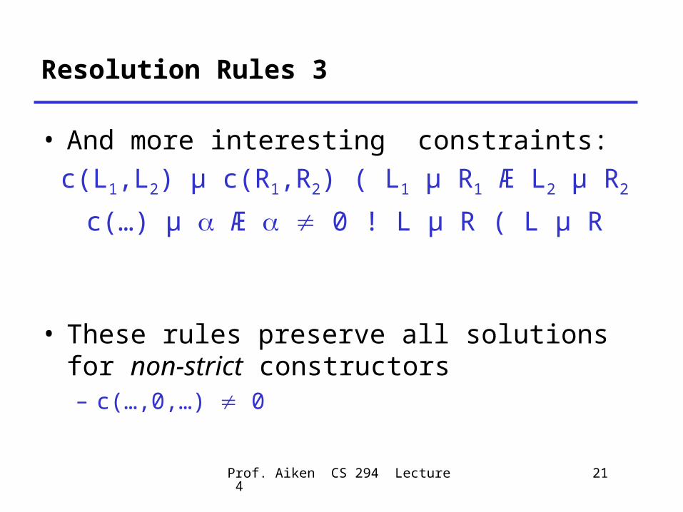
Resolution Rules 3
• And more interesting constraints:c(L1,L2) µ c(R1,R2) ( L1 µ R1 Æ L2 µ R2
c(…) µ Æ 0 ! L µ R ( L µ R
• These rules preserve all solutions for non-strict constructors– c(…,0,…) 0

Prof. Aiken CS 294 Lecture 4 22
Resolution Rules 4
• Note how the rules preserve R and L:c(L1,L2) µ c(R1,R2) ( L1 µ R1 Æ L2 µ R2
• We can also have constructors with contravariant arguments; e.g., !
L ::= … | R ! LR ::= … | L ! R
R1 ! L1 µ L2 ! R2 , L2 µ R1 Æ L1 µ R2

Prof. Aiken CS 294 Lecture 4 23
An Observation
• Note the resolution rules do not create new expressions– Only subexpressions are used– E.g.,
Lµ R1 Å R2 , L µ R1 Æ L µ R2
L1 [ L2 µ R , L1 µ R Æ L2 µ R
c(…) µ Æ µ R , c(…) µ Æ µ R Æ c(…) µ R
Prof. Aiken CS 294 Lecture 4 24
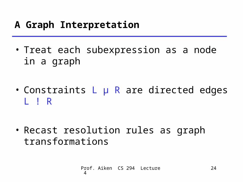
A Graph Interpretation
• Treat each subexpression as a node in a graph
• Constraints L µ R are directed edges L ! R
• Recast resolution rules as graph transformations

Prof. Aiken CS 294 Lecture 4 25
Resolution on Graphs 1
c(…) µ Æ µ R , c(…) µ Æ µ R Æ c(…) µ R
Rc(…)

Prof. Aiken CS 294 Lecture 4 26
Resolution on Graphs 2
c(…) µ Æ 0 ! L µ R ( L µ R
c(…)
L R

Prof. Aiken CS 294 Lecture 4 27
Resolution on Graphs 3
c(L1,L2) µ c(R1,R2) ( L1 µ R1 Æ L2 µ R2
L1
c(L1,L2)
L2 R1
c(R1,R2)
R2

Prof. Aiken CS 294 Lecture 4 28
The Other Constraints
• Skip presentation of rules for other constraints– Trivial constraints– Intersection/union constraints
• Easily handled– In practice, edges from these constraints are
not explicitly represented anyway– Tend to keep only constraints on variables

Prof. Aiken CS 294 Lecture 4 29
Notes
• The process of adding edges according to a set of rules is called closing the graph
• The closed graph gives the solution of the constraints

Prof. Aiken CS 294 Lecture 4 30
Algorithmics
• This algorithm is a dynamic transitive closure
• New edges other than transitive edges are added during the closure procedure
• Can’t use standard transitive closure tricks– E.g., Boolean matrix multiplication

Prof. Aiken CS 294 Lecture 4 31
Dynamic Transitive Closure
• The best known algorithms for dynamic transitive closure are O(n3)– Has not been improved in 30 years
• Sketch: In the worst case, a graph of n nodes– May have n2 edges– Each edge may be added O(n) times

Prof. Aiken CS 294 Lecture 4 32
Applications

Prof. Aiken CS 294 Lecture 4 33
Four Applications
• Closure analysis for lambda calculus• Receiver class analysis for OO languages• Alias analysis for C

Prof. Aiken CS 294 Lecture 4 34
Closure Analysis: The Problem
• A call graph is a graph where– The nodes are function (method) names– There is a directed edge (f,g) if f may call g
• Call graphs can be overestimates– If f may call g at run time, there must be an
edge (f,g) in the call graph– If f cannot call g at run time, there is no
requirement on the graph

Prof. Aiken CS 294 Lecture 4 35
Call Graphs in Functional Languages
• Recall the untyped lambda calculus:
e = x | x.e | e e
• Examples:– ((x.x) (y.y)) (z.z)– ((x.y.y) (z.z)) (w.w)– (x.x x) (y.y y)

Prof. Aiken CS 294 Lecture 4 36
A Definition
• Assume all bound variables are unique– So a bound variable uniquely identifies a function– Can be done by renaming variables
• For each application e1 e2, what is the set of lambda terms L(e1) to which e1 may evaluate?– L(…) is a set of static, or syntactic, lambdas– L(…) defines a call graph
• the set of functions that may be called by an application

Prof. Aiken CS 294 Lecture 4 37
A More General Definition
• To compute L(…) for applications, we will need to compute it for every expression.
• Define:L(e) is the set of syntactic lambda
abstractions to which e may evaluate
• The problem is to compute L(e) for every expression e

Prof. Aiken CS 294 Lecture 4 38
Defining L(…)
x.eL(x.e) = x.e
e1 e2
for each x.e 2 L(e1)
L(e2) µ L(x)
L(e) µ L(e1 e2)The value of the application includes the value of the function body
The actual argument of the call flows to the formal argument

Prof. Aiken CS 294 Lecture 4 39
Rephrasing the Constraints with µ
The following constraints have the same least solution as the original constraints:
x.ex.e µ L(x.e)
e1 e2
x.e0 µ L(e1) ) (L(e2) µ L(x) Æ L(e0) µ L(e1 e2))
Note: Each L(e) is a constraint variable Each x.e is a constant

Prof. Aiken CS 294 Lecture 4 40
Example ((x.x) (y.y)) (z.z)
x.x µ L(x.x)y.y µ L(y.y)z.z µ L(z.z) L(y.y) µ L(x)
L(x) µ L((x.x) (y.y)) L(z.z) µ L(y)
L(y) µ L(((x.x) (y.y)) (z.z))
Least solution:L(x.x) = x.xL(y.y) = y.yL(z.z) = z.z
L(y.y) = L(x) = L((x.x) (y.y)) L(z.z) = L(y) = L(((x.x) (y.y))
(z.z))

Prof. Aiken CS 294 Lecture 4 41
The Example ((x.x) (y.y)) (z.z) with Graphs
z
z.zy
y.yx x.x
(x.x) (y.y)
((x.x) (y.y)) (z.z)
x.xy.y
z.z

Prof. Aiken CS 294 Lecture 4 42
The Solution for ((x.x) (y.y)) (z.z)
z
z.zy
y.yx x.x
(x.x) (y.y)
((x.x) (y.y)) (z.z)
The solution is given by edges (x.e,*)
x.x
z.z
y.y

Prof. Aiken CS 294 Lecture 4 43
Control Flow Graphs in OO Languages
• Consider a method call e0.f(e1,…,en)
• To build a control-flow graph, we need to know which f methods may be called– Depends on the class of e0 at runtime
• The problem:– For each expression, estimate the set of classes
it could evaluate to at run time

Prof. Aiken CS 294 Lecture 4 44
An OO Language
P ::= C1 . . . Cn E
C ::= class ClassId [inherits ClassId]var Id1 . . . Idk M1 . . . Mn
M ::= method MId(Id) E
E ::= Id := E | E.MId(E,…,E) | E;E | new ClassId |
if E E E

Prof. Aiken CS 294 Lecture 4 45
Constraints
id := eC(e) µ C(id)C(e) µ C(id := e)
e1; e2
C(e2) µ C(e1; e2)
new A{ A } µ C(new A)
if e1 e2 e3
C(e2) µ C(if e1 e2 e3)
C(e3) µ C(if e1 e2 e3)
e0.f(e1)
for each class A with a method f(x) eA 2 C(e0) )
C(e1) µ C(x) Æ
C(e) µ C(e0.f(e1))

Prof. Aiken CS 294 Lecture 4 46
Notes
• Receiver class analysis of OO languages and control flow analysis of functional languages are the same problem
• Receiver class analysis is important in practice– Heavily object-oriented code pays a high price for
the indirection in method calls– If we can show that only one method can be
called, the function can be statically bound• Or even inlined and optimized

Prof. Aiken CS 294 Lecture 4 47
Type Safety
• Notice that our OO language is untyped– We can run (new A).f(0) even if A has no f
method– Gives a runtime error
• By adding upper bounds to the constraints, we can make receiver class analysis into a type inference procedure for our language

Prof. Aiken CS 294 Lecture 4 48
Type Inference
id := eC(e) µ C(id)C(e) µ C(id := e)
e1; e2
C(e2) µ C(e1; e2)
new A{ A } µ C(new A)
if e1 e2 e3
C(e2) µ C(if e1 e2 e3)
C(e3) µ C(if e1 e2 e3)
C(e1) µ { Bool }
e0.f(e1)
for each class A with a method f(x) e
A 2 C(e0) )
C(e1) µ C(x) Æ
C(e) µ C(e0.f(e1))
C(e0) µ { A | A has an f
method }
Prof. Aiken CS 294 Lecture 4 49
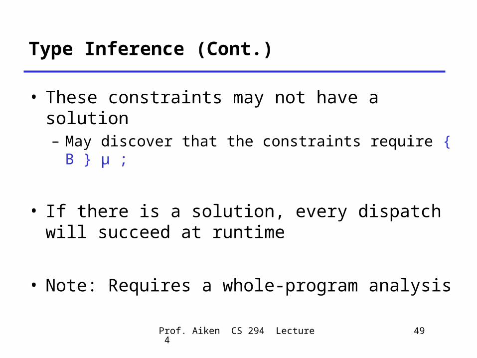
Type Inference (Cont.)
• These constraints may not have a solution– May discover that the constraints require { B }
µ ;
• If there is a solution, every dispatch will succeed at runtime
• Note: Requires a whole-program analysis

Prof. Aiken CS 294 Lecture 4 50
Alias Analysis (Review)
• In languages with side effects, want to know which locations may have aliases– More than one “name”– More than one pointer to them
• E.g.,Y = &ZX = Y*X = 3 /* changes the value of *Y */

Prof. Aiken CS 294 Lecture 4 51
Alias Analysis: An Improvement
• The unification-based analysis we saw in Lecture 3 is coarse
• Points-to sets are equivalence classes
• Inclusion-based analysis can be more accurate
Prof. Aiken CS 294 Lecture 4 52
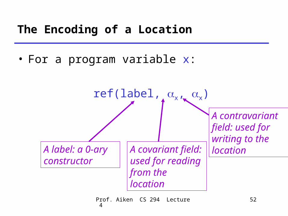
The Encoding of a Location
• For a program variable x:
ref(label, x, x)
A label: a 0-ary constructor
A covariant field: used for reading from the location
A contravariant field: used for writing to the location

Prof. Aiken CS 294 Lecture 4 53
Inference Rules
1 1 2 2
1
2
1 2 2
:: ( , , ) & : (0, , )
: :
(1,1, ) f resh:
(1, ,0) (1, ,0) f resh
f resh
* : :
x x x
ex refl e ref
e e
refe
ref ref
e e e

Prof. Aiken CS 294 Lecture 4 54
In Practice
• Many natural inclusion-based analysis problems are equivalent to dynamic transitive closure
• Widely believed to be impractical– O(n3) suggests it may be slow– And in fact it is
• Many implementations have tried

Prof. Aiken CS 294 Lecture 4 55
One Problem
• Consider what happens on a cycle in the graph
• A constructed lower bound on any one node is propagated to every node in the cycle
c(…)
Prof. Aiken CS 294 Lecture 4 56
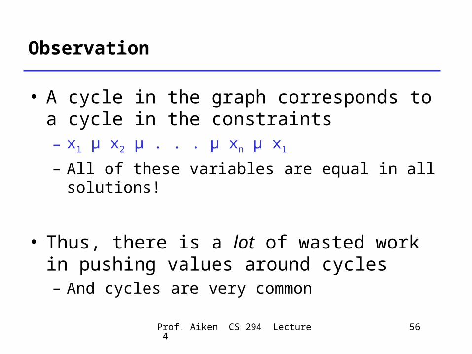
Observation
• A cycle in the graph corresponds to a cycle in the constraints– x1 µ x2 µ . . . µ xn µ x1
– All of these variables are equal in all solutions!
• Thus, there is a lot of wasted work in pushing values around cycles– And cycles are very common

Prof. Aiken CS 294 Lecture 4 57
The Idea
• We want to detect and eliminate cycles on-line– Collapse cycles to a single node– During constraint resolution
• On-line cycle detection is very hard– No known algorithm is significantly better than
stopping the graph closure and doing a depth-first search of the entire graph

Prof. Aiken CS 294 Lecture 4 58
Partial On-Line Cycle Elimination
• Instead, we will settle for partial cycle elimination– For every cycle that exists in the graph,
guarantee we find at least a piece of it– And do it cheaply

Prof. Aiken CS 294 Lecture 4 59
A Different Representation
• We change the representation of the graph– Assign every variable x (node) arbitray index
R(x)– Each node has a list of edges stored with it– An edge (x,y) is stored
• At x if R(x) > R(y) (a successor edge, colored red)• At y if R(y) > R(x) (a predecessor edge, colored blue)
• New transitive closure rule:

Prof. Aiken CS 294 Lecture 4 60
Cycle Detection Algorithm
• On each edge addition (x,y)– If (x,y) is a successor edge (R(x) > R(y)) then
search along predecessor edges from x. • When a node z s.t. R(z) < R(y) is found, prune that path• If y is found, a cycle is detected
– If (x,y) is a predecessor edge (R(x) < R(y)) then search along successor edges from y.
• When a node z s.t. R(z) < R(x) is found, prune that path• If x is found, a cycle is detected

Prof. Aiken CS 294 Lecture 4 61
Cycle Detection in Pictures
57 22
45
917
42

Prof. Aiken CS 294 Lecture 4 62
Part of Every Cycle is Detected
• Every cycle has at least one red and one blue edge– Indices cannot uniformly increase or decrease
around a cycle
• Thus, the transitivity rule always applies– Always adds a chord across the cycle, giving a
smaller cycle
• Two-cycles are always detected 57 22
9942

Prof. Aiken CS 294 Lecture 4 63
Analysis of Cycle Detection
• Part of every cycle is detected
• Expected number of nodes visited per edge addition is very low– About 2, in theory– Why? Long chains of descending, arbitrarily
chosen indices are very unlikely
• Can show asymptotic speedup in graph closure for random graphs

Prof. Aiken CS 294 Lecture 4 64
Experiments
• Cycle detection is fast– In experiments, 1.8 nodes visited/edge addition– Constants are very small
• About 80% of nodes in cycles are detected– Detected cycles are removed from the graph and
put in a union/find data structure
• Gives asymptotic performance improvement– For alias analysis of C
• Allows programs 10X larger to be analyzed than without

Prof. Aiken CS 294 Lecture 4 65
Summary
• Dynamic transitive closure algorithms are coming– Still “in the lab”, but increasingly practical– Need more tricks than cycle elimination

Prof. Aiken CS 294 Lecture 4 66
Summary of Constraint-Based Analysis
• Constraints separate– Specification (system of constraints)– Implementation (constraint resolution)
• Clear place to apply algorithmic knowledge
• No forwards-backwards distinction– Can solve for any unknown
• Infinite domains• Separate analysis is easy
– Can always solve constraints

Prof. Aiken CS 294 Lecture 4 67
Where is Constraint-Based Analysis Weak?
• Only fairly simple constraints are practical– This situation is improving
• Doesn’t capture all of abstract interpretation– In particular, situations where there is a favored
direction (forwards, backwards) for efficiency reasons

Prof. Aiken CS 294 Lecture 4 68
Things We Didn’t Talk About
• Polymorphism– Context-free reachability & polymorphic recursion
• Effect Systems– A computation has a type & an effect– E.g., the set of memory locations written– Mixed constraint systems
• Other constraint languages– There are some besides = and µ