Produzione e Validazione dei campi Meteorologici nell’ambito del progetto MINNI
27
Produzione e Validazione dei campi Meteorologici nell’ambito del progetto MINNI Lina Vitali , Massimo D’Isidoro ENEA- UTVALAMB-AIR Incontro ENEA – LaMMA Bologna, 27 settembre 2012
-
Upload
phoebe-sykes -
Category
Documents
-
view
41 -
download
2
description
Produzione e Validazione dei campi Meteorologici nell’ambito del progetto MINNI. Lina Vitali , Massimo D’Isidoro ENEA- UTVALAMB-AIR Incontro ENEA – LaMMA Bologna, 27 settembre 2012. Il Progetto MINNI. La catena Modellistica. - PowerPoint PPT Presentation
Transcript of Produzione e Validazione dei campi Meteorologici nell’ambito del progetto MINNI
Produzione e Validazione dei campi Meteorologici nell’ambito del progetto
MINNILina Vitali , Massimo D’Isidoro
ENEA- UTVALAMB-AIR
Incontro ENEA – LaMMA Bologna, 27 settembre 2012
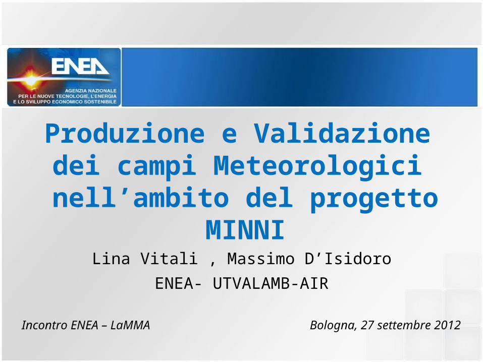
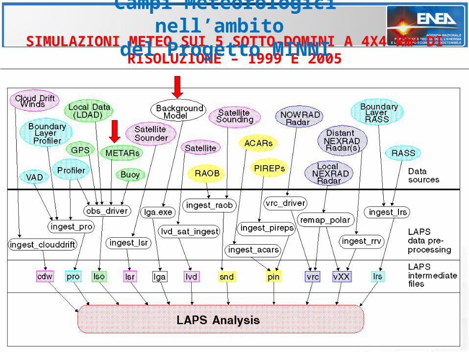
RAMS, LAPS
Emission Manager
SURFPRO
Meteo
Parametri di turbolenza
FARM
Emissioni
Campi ECMWF Dati Locali Inventari
(ISPRA ed EMEP)
Info spaziali e temporali
Concentrazioni e Deposizioni
Matrici di
Trasferimento
Campi EMEP
IC e BC
Sottosistema METEO Sottosist
ema EMISSIVO
Sottosistema CHIMICO-FISICO
GAINS
LA CATENA MODELLISTICA
Il Progetto MINNI
http://www.minni.org/
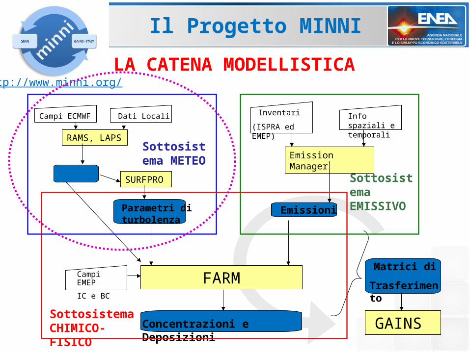
1999, 200520km : RAMS (nudging)4km : LAPS
2003, 200720 km : RAMS (nudging) 4km : RAMS (nudging)
APPROCCIO MODELLISTICO PER LA METEOROLOGIA
Il Progetto MINNI
http://www.minni.org/
DOMINI
SIMULAZIONI METEO SUL DOMINIO NAZIONALE A 20X20 km2 DI RISOLUZIONE
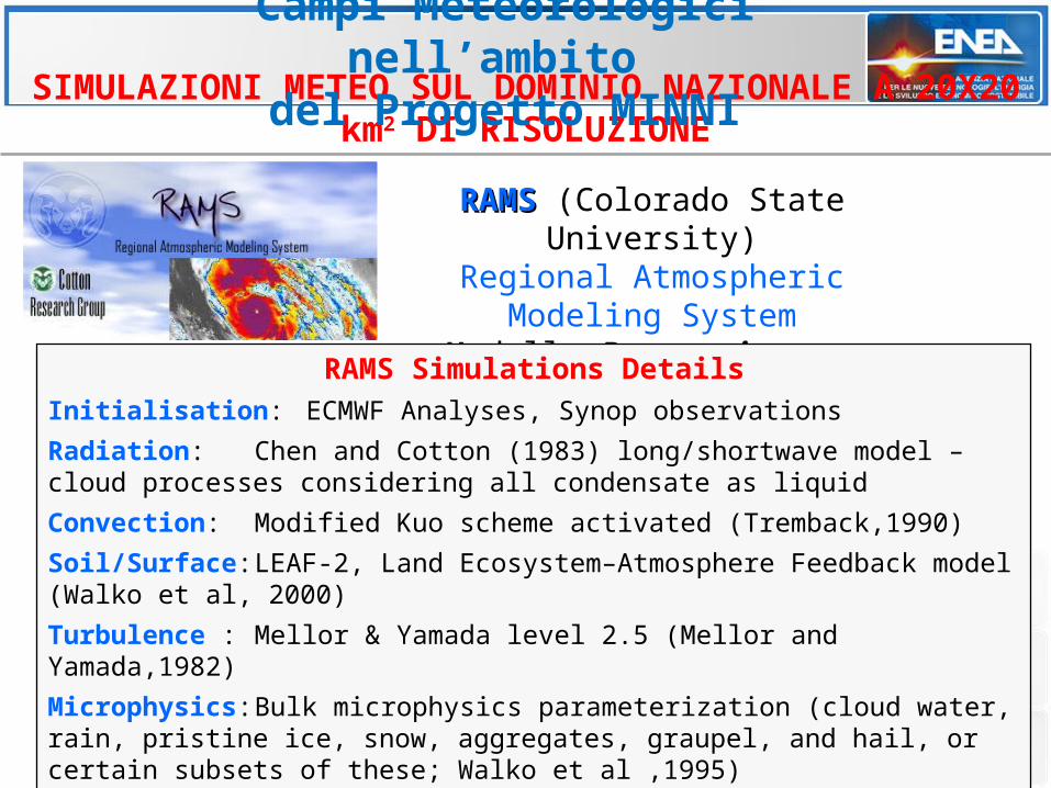
RAMSRAMS (Colorado State University)
Regional Atmospheric Modeling System
Modello Prognostico non idrostatico
Campi Meteorologici nell’ambito
del Progetto MINNI
RAMS Simulations DetailsInitialisation: ECMWF Analyses, Synop observations
Radiation: Chen and Cotton (1983) long/shortwave model – cloud processes considering all condensate as liquid
Convection: Modified Kuo scheme activated (Tremback,1990)
Soil/Surface: LEAF-2, Land Ecosystem–Atmosphere Feedback model (Walko et al, 2000)
Turbulence : Mellor & Yamada level 2.5 (Mellor and Yamada,1982)
Microphysics: Bulk microphysics parameterization (cloud water, rain, pristine ice, snow, aggregates, graupel, and hail, or certain subsets of these; Walko et al ,1995)
4DDA: Nudging on pre-analysed fields
Archiving: Fields archived on houly basis.
celina
ISWRTYPintegerFlag specifying options for evaluating shortwave radiative transfer in themodel (0 = no radiation, 1 = Chen and Cotton parameterization, 2 = Mahrerand Pielke parameterization, 3 = two-stream parameterization developed byHarrington).The Mahrer and Pielke scheme is the simplest and by far the leastexpensive computationally. The main reason for this is that it ignores liquidand ice in the atmosphere, although it does account for water vapor. Thisscheme should not be used, for example, if attenuation of solar radiation byclouds is important to the simulation.The Chen and Cotton scheme does account for condensate in theatmosphere, but not whether it is cloud water, rain, or ice. This is a majorlimitation.The Harrington parameterization accounts for each form of condensate(cloud water, rain, pristine ice, snow, aggregates, graupel, and hail) as wellas water vapor, and even utilizes information on ice crystal habit. Inaddition, the scheme adds upper atmospheric levels for radiationcomputation for cases where the model domain does not extend up to atleast 25 km (roughly the height of the ionosphere). This is the mostsophisticated parameterization and is recommended over the Chen andCotton scheme. It is, however, still the most computationally expensivescheme, although work is planned to improve its performance. (See alsoILWRTYP and RADFRQ.)
celina
Grid-dependent flag used to select the convective parameterization is to beactivated or not.NNQPARM = 0 – no convective parameterization for the grid.NNQPARM = 1 – the Kuo-type parameterization will be run for the grid.NNQPARM = 2 – the Kain-Fritsch parameterization will be run for the grid(requires LEVEL=3).Convective parameterization is used to vertically redistribute heat andmoisture (as if by convection) in a grid column when the model generates aregion which is superadiabatic or convectively unstable and when thehorizontal grid resolution is too coarse for the model to develop its ownconvective circulation. Ideally, resolving a convective circulation wouldrequire at least a few grid cells to horizontally span an updraft, which fordeep convection would normally require the horizontal cell size to be lessthan 1 or 2 kilometers. Coarser resolution than this would make realizationof sufficiently strong vertical motion difficult or impossible to adequately bringabout the required vertical exchange of heat and moisture so as to convertthe convective available potential energy into other forms. Thus, it is oncoarser grids where a parameterized convective adjustment becomesnecessary. Unfortunately, the convective parameterization schemescurrently available assume the grid size in the horizontal to be around 20kilometers or greater. This means that convective parameterization may beactivated on any grid of this resolution, but that at resolutions between about2 and 20 kilometers, no adequate convective adjustment scheme exists.
celina
RAMS implements also a land ecosystem-atmosphere feedback module (LEAF-2, Land Ecosystem–Atmosphere Feedback model, Walko et al, 2000) for the evaluation of energy and water budgets and fluxes, so multiple layers prognostic equations for soil temperature and moisture are also included . As for the initial soil status, Toto limit initialization influence, the initial soil status,profiles for on January 1st at 00 UTC, has have been obtained from a preliminary model simulation extended to the whole month of December in the previous year. The subsequent simulations have been initialized from the 3D soil fields produced by the previous week's simulation, allowing continuity of soil status during the whole yearly model run.
celina
Grid-dependent flag that controls the type of parameterization to be used forcomputing both horizontal and vertical diffusion coefficients. Allowablevalues for this flag are 1, 2, 3, or 4. A value of 1 or 2 is appropriate to modelgrids in which the horizontal grid spacing is large compared to the verticalspacing such that dominant convective motions are not resolved. Horizontaldiffusion in such cases is normally required to be stronger (for numericaldamping) than justifiable on physical grounds, and the model assumescomplete decoupling of the horizontal and vertical diffusion in all aspects,including computation of deformation rates, length scales, and stress tensorcomponents.IDIFFK = 1 or 2 - the horizontal diffusion coefficients are computed as theproduct of horizontal deformation rate (horizontal gradients of horizontalvelocity) and a length scale squared, based on the original Smagorinskyformulation. The length scale is the product of x-direction grid spacingDELTAX and namelist parameter CSX.IDIFFK = 1 - vertical diffusion is parameterized according to the Mellor andYamada scheme, which employs a prognostic turbulent kinetic energy(TKE).IDIFFK = 2 - vertical diffusion is computed from a 1-dimensional analog ofthe Smagorinsky scheme in which vertical deformation is evaluated fromvertical gradients of horizontal wind, and vertical length scale is the localvertical grid spacing times namelist parameter CSZ. In addition,modifications of the vertical diffusion coefficient due to static stability orinstability are used, based on formulations of Hill and Lilly. The Lillymodification is in the form of a multiplying factor, equal to sqrt(1-R kh/km)where R is the Richardson number and kh/km is the ratio of the scalar tomomentum vertical diffusion coefficients specified by the user in namelistvariable ZKHKM . The multiplying factor is greater than 1 in unstable cases(i.e., where wind shear and/or unstable lapse rates make the Richardsonnumber sufficiently low, and is less than 1 in stable cases. The Hillmodification applies only to regions of unstable lapse rates (having negativesquared Brunt-Vaisala frequencies), and consists of adding the absolutevalue of the Brunt-Vaisala frequency squared to the deformation rate, toobtain a modified inverse time scale for the diffusion coefficient computation.The Lilly and Hill modifications were originally designed for use without eachother, although we have found that the added vertical diffusion in unstableair obtained by using both together is usually desirable.Values of 3, 4, 5, or 6 for IDIFFK are usually appropriate on grids havingcomparable horizontal and vertical spacings, and are intended for use insituations where dominant 3-dimensional motions, such as cumulus orboundary layer convection, are resolved. In these cases, RAMS computesdiffusion coefficients from the 3-dimensional rate-of-strain tensor, and usesthe same or similar diffusion coefficients for horizontal and vertical diffusion.IDIFFK = 3 - horizontal and vertical diffusion coefficients are computed asthe product of the 3-D rate-of-strain tensor and a length scale squared. Thelength scale is the product of the vertical grid spacing and namelistparameter CSZ. The Hill and Lilly stability-dependent modificationsdescribed above also apply to IDIFFK set to 3.IDIFFK = 4 - vertical and horizontal diffusion are parameterized according tothe Deardorff scheme, which employs a prognostic subgrid turbulent kineticenergy. This scheme is intended only for the specific purpose of performinga large eddy simulation (LES) in which it is assumed that resolved eddymotions in the model perform most of the eddy transport. Theparameterized diffusion only represents the subgrid turbulent mixing. Thus,the Deardorff scheme is not appropriate for horizontal grid cell sizes largerthan a couple hundred meters. In both the Deardorff and Mellor andYamada schemes, the prognostic kinetic energy is generated by means ofshear and buoyancy processes, and a parameterized pressure-work term,and is destroyed by potentially all of the above plus a parameterizeddissipation term. The kinetic energy is also advected and diffused. Theresult of these processes yields a field of kinetic energy from which thediffusion coefficients are locally diagnosed.IDIFFK = 5 – E-l isotropic schemeIDIFFK = 6 – E-� isotropic scheme
celina
LEVELintegerFlag that specifies the level of moisture complexity to be activated in themodel. This flag is the primary means by which the user tells the modelwhether to consider the effects of moisture in the simulation, and if so, towhat degree.LEVEL = 0 - causes the model to run dry, completely eliminating anyprocess which influences or is influenced by any phase of moisture. Withthis option, radiation parameterizations (controlled by ISWRTYP andILWRTYP) must be turned off.LEVEL = 1 - activates advection, diffusion, and surface flux of water, whereall water substance in the atmosphere is assumed to occur as vapor even ifsupersaturation occurs. The value of 1 also activates the buoyancy effect ofwater vapor in the vertical equation of motion, as well as the radiative effectsof water vapor if radiation is activated elsewhere.LEVEL = 2 - activates condensation of water vapor to cloud water whereversupersaturation is attained. The partitioning of the total water substance intovapor and cloud water is purely diagnostic in this case. No other forms ofliquid or ice water are considered. Both the positive buoyancy effect ofwater vapor and the liquid water loading of cloud water are included in thevertical equation of motion. Radiative effects of both water vapor and cloudwater are activated, if the radiation parameterization is itself activated.LEVEL = 3 - activates the bulk microphysics parameterization, whichincludes cloud water, rain, pristine ice, snow, aggregates, graupel, and hail,or certain subsets of these as specified by ICLOUD, IRAIN, IPRIS, ISNOW,IAGGR, IGRAUP, and IHAIL. This parameterization includes theprecipitation process.Dal RAMSIN!----- Microphysics ------------------------------------------------------ LEVEL = 3, ! Moisture complexity level ICLOUD = 4, ! Microphysics flags IRAIN = 2, !------------------- IPRIS = 5, ! 1 - diagnostic concen. ISNOW = 2, ! 2 - specified mean diameter IAGGR = 2, ! 3 - specified y-intercept IGRAUP = 2, ! 4 - specified concentration IHAIL = 2, ! 5 - prognostic concentration CPARM = .3e9, ! Microphysics parameters RPARM = 1e-3, !------------------------- PPARM = 0., ! Characteristic diameter, # concentration SPARM = 1e-3, ! or y-intercept APARM = 1e-3, GPARM = 1e-3, HPARM = 3e-3, GNU = 2.,2.,2.,2.,2.,2.,2., ! Gamma shape parms for ! cld rain pris snow aggr graup hail!-----------------------------------------------------------------------------
SIMULAZIONI METEO SUL DOMINIO NAZIONALE A 20X20 km2 DI RISOLUZIONE
RAMSRAMS (Colorado State University)
Regional Atmospheric Modeling System
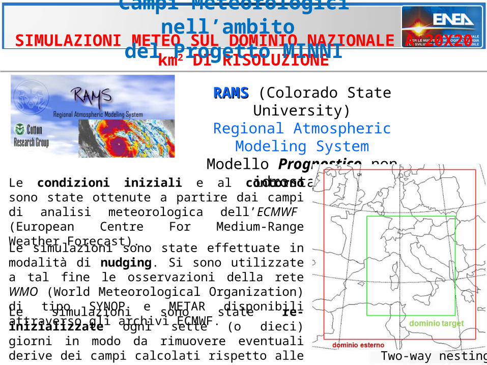
Modello Prognostico non idrostaticoLe condizioni iniziali e al contorno sono
state ottenute a partire dai campi di analisi meteorologica dell’ECMWF (European Centre For Medium-Range Weather Forecast).
Le simulazioni sono state effettuate in modalità di nudging. Si sono utilizzate a tal fine le osservazioni della rete WMO (World Meteorological Organization) di tipo SYNOP e METAR disponibili attraverso gli archivi ECMWF. Le simulazioni sono state re-inizializzate ogni sette (o dieci) giorni in modo da rimuovere eventuali derive dei campi calcolati rispetto alle analisi di grande scala e alle osservazioni locali.
Campi Meteorologici nell’ambito
del Progetto MINNI
Two-way nesting.

LAPS (Local Analysis and Prediction System)
Modello Diagnostico
SIMULAZIONI METEO SUI 5 SOTTO-DOMINI A 4X4 km2 DI RISOLUZIONE – 1999 E 2005
Campi Meteorologici nell’ambito
del Progetto MINNI
SIMULAZIONI METEO SUI 5 SOTTO-DOMINI A 4X4 km2 DI RISOLUZIONE – 1999 E 2005
Campi Meteorologici nell’ambito
del Progetto MINNI
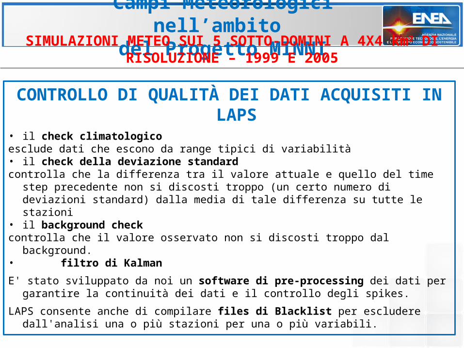
CONTROLLO DI QUALITÀ DEI DATI ACQUISITI IN LAPS
• il check climatologico esclude dati che escono da range tipici di variabilità• il check della deviazione standard controlla che la differenza tra il valore attuale e quello del time step
precedente non si discosti troppo (un certo numero di deviazioni standard) dalla media di tale differenza su tutte le stazioni
• il background check controlla che il valore osservato non si discosti troppo dal background.• filtro di Kalman
E' stato sviluppato da noi un software di pre-processing dei dati per garantire la continuità dei dati e il controllo degli spikes.
LAPS consente anche di compilare files di Blacklist per escludere dall'analisi una o più stazioni per una o più variabili.
Campi Meteorologici nell’ambito
del Progetto MINNISIMULAZIONI METEO SUI 5 SOTTO-DOMINI A 4X4 km2 DI RISOLUZIONE – 1999 E 2005
Campi Meteorologici nell’ambito
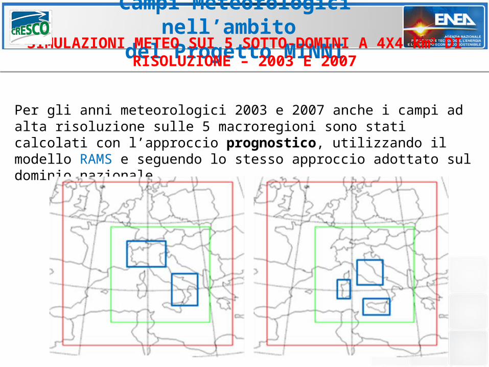
del Progetto MINNISIMULAZIONI METEO SUI 5 SOTTO-DOMINI A 4X4 km2 DI RISOLUZIONE – 2003 E 2007
Per gli anni meteorologici 2003 e 2007 anche i campi ad alta risoluzione sulle 5 macroregioni sono stati calcolati con l’approccio prognostico, utilizzando il modello RAMS e seguendo lo stesso approccio adottato sul dominio nazionale.
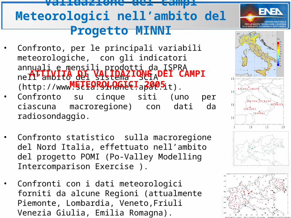
• Confronto, per le principali variabili meteorologiche, con gli indicatori annuali e mensili prodotti da ISPRA nell’ambito del sistema SCIA (http://www.scia.sinanet.apat.it).
Validazione dei campi Meteorologici nell’ambito del
Progetto MINNI
5 1 0 1 5 2 0
3 6
4 0
4 4
4 8
B R I N D I S I
T R A P A N I
C A G L I A R I
M I L A N O _ L I N A T E
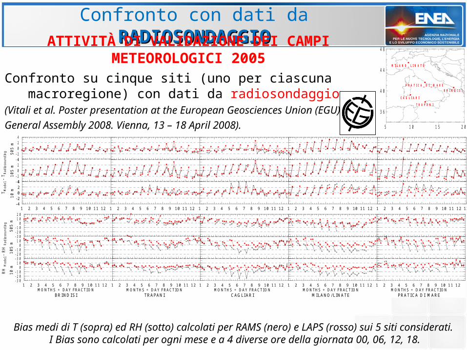
P R A T I C A _ D I _ M A R E• Confronto su cinque siti (uno per ciascuna
macroregione) con dati da radiosondaggio.
• Confronti con i dati meteorologici forniti da alcune Regioni (attualmente Piemonte, Lombardia, Veneto,Friuli Venezia Giulia, Emilia Romagna). Confronti orari su ciascuna stazione.(già a disposizione i dati anche per il 2003 e il 2007)
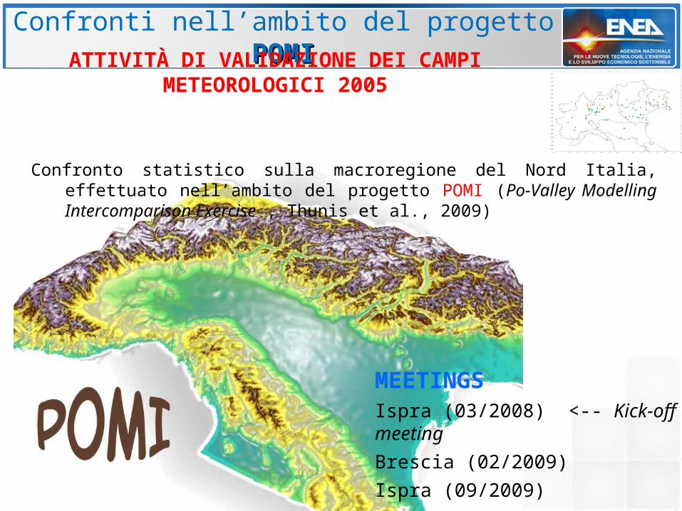
• Confronto statistico sulla macroregione del Nord Italia, effettuato nell’ambito del progetto POMI (Po-Valley Modelling Intercomparison Exercise ).
ATTIVITÀ DI VALIDAZIONE DEI CAMPI METEOROLOGICI 2005
5 1 0 1 5 2 0
3 6
4 0
4 4
4 8
B R I N D I S I
T R A P A N I
C A G L I A R I
M I L A N O _ L I N A T E
P R A T I C A _ D I _ M A R E
1 2 3 4 5 6 7 8 9 10 11 12- 4- 2024
10
m
- 4- 2
024
10
5 m
- 4- 2
024
50
5 m
TM
od
el -
TR
adio
sou
nd
ing
1 2 3 4 5 6 7 8 9 10 11 12 1 2 3 4 5 6 7 8 9 10 11 12 1 2 3 4 5 6 7 8 9 10 11 12 1 2 3 4 5 6 7 8 9 10 11 12 13
1 2 3 4 5 6 7 8 9 10 11 12MO NTHS + DAY FRACTI O N
BR I NDI S I
- 30- 20- 10
010
10
m
- 30- 20- 10
010
10
5 m
- 30- 20- 10
01020
50
5 m
RH
Mod
el -
RH
Rad
ioso
un
din
g
1 2 3 4 5 6 7 8 9 10 11 12MONTHS + DAY FRACTI ON
TRAPANI
1 2 3 4 5 6 7 8 9 10 11 12MO NTHS + DAY FRACTI O N
CAGLI AR I
1 2 3 4 5 6 7 8 9 10 11 12MONTHS + DAY FRACTI ON
MI LANO/ LI NATE
1 2 3 4 5 6 7 8 9 10 11 12MONTHS + DAY FRACTI ON
PRATI CA DI MARE
Bias medi di T (sopra) ed RH (sotto) calcolati per RAMS (nero) e LAPS (rosso) sui 5 siti considerati.
I Bias sono calcolati per ogni mese e a 4 diverse ore della giornata 00, 06, 12, 18.
Confronto con dati da RADIOSONDAGGIORADIOSONDAGGIO
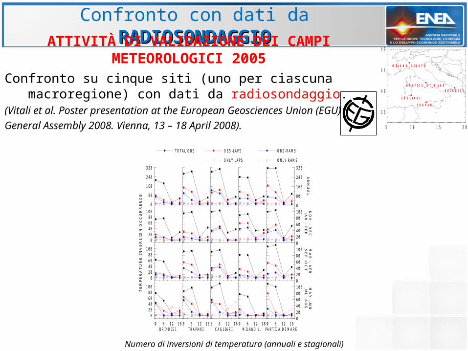
Confronto su cinque siti (uno per ciascuna macroregione) con dati da radiosondaggio.
(Vitali et al. Poster presentation at the European Geosciences Union (EGU)
General Assembly 2008. Vienna, 13 – 18 April 2008).
ATTIVITÀ DI VALIDAZIONE DEI CAMPI METEOROLOGICI 2005
celina
Confronto importante visto che non c'è stata assimilazione in verticale.Confronto su tre livelli di FARM (vecchia struttura verticale). sopra LAPS non corregge più.Temperatura: In superficie LAPS tende a ridurre i bias massimi, soprattutto nei mesi caldi e nelle ora più calde della giornata. Alle quote superiori invece LAPS non introduce sostanziali miglioramenti.Umidità Relativa: In superficie LAPS tende a ridurre la sottostima nei mesi caldi, in tutti i siti, portando però talvolta a una sovrastima (a Brindisi e a pratica di Mare). A 105 m si osserva un generale passaggio dalla sottostima alla sovrastima.A 505 m le uniche significative correzioni si osservano a Milano Linate a mezzogiorno.
5 1 0 1 5 2 0
3 6
4 0
4 4
4 8
B R I N D I S I
T R A P A N I
C A G L I A R I
M I L A N O _ L I N A T E
P R A T I C A _ D I _ M A R E
Confronto con dati da RADIOSONDAGGIORADIOSONDAGGIO
0 6 12 18BR I ND I S I
020406080
100
0 6 12 18TRA PA NI
0 6 12 18CAGLI A R I
0 6 12 18MI LA NO L.
0 6 12 18PA RT I CA D I MA RE
020406080100 M
AY
-JUN
JUL -A
UG
020406080
100
TE
MPE
RA
TU
RE
IN
VE
RS
ION
OC
CU
RR
EN
CE
020406080100 M
AR
- APR
SE
P -OC
T
020406080
100
020406080100 N
OV
- DE
CJA
N - F
EB
0
80
160
240
320
0
80
160
240
320
AN
NU
AL
TOTAL OBS
ONLY RAMS
OBS - RAMS
ONLY LAPS
OBS - LAPS
Numero di inversioni di temperatura (annuali e stagionali)
ATTIVITÀ DI VALIDAZIONE DEI CAMPI METEOROLOGICI 2005
Confronto su cinque siti (uno per ciascuna macroregione) con dati da radiosondaggio.
(Vitali et al. Poster presentation at the European Geosciences Union (EGU)
General Assembly 2008. Vienna, 13 – 18 April 2008).
celina
The annual and seasonal number of occurrence of T inversion over the 5 sites. The number of occurrence derived by radiosounding are shown by black lines: the red and blue continuous lines with filled circles show the number of occurrence detected by both LAPS and soundings and by both RAMS and soundings. Red and blue dashed lines represent respectively the LAPS and RAMS number of occurrence of T inversion do not corresponding with the observed ones. Il maggior numero di inversioni avviene di notte.ATTENZIONE : probabile sottostima nel numero di inversioni osservate alle 18. Dati a disposizione: solo 3 mesi a Trapani e a Cagliari, 2 mesi a Milano Linate e a Pratica di Mare, nessuno a Brindisi. Ad entrambe le risoluzioni è sottostimato il numero delle inversioni ma LAPS riduce la sottostima.Unica eccezione: Cagliari a mezzanotte.Buona notizia: la minore sottostima si ha a Milano d’inverno.LAPS genera più frequentemente casi di “false inversioni”.
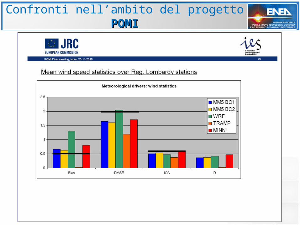
Confronto statistico sulla macroregione del Nord Italia, effettuato nell’ambito del progetto POMI (Po-Valley Modelling Intercomparison Exercise , Thunis et al., 2009)
Confronti nell’ambito del progetto POMIPOMIATTIVITÀ DI VALIDAZIONE DEI CAMPI
METEOROLOGICI 2005
MEETINGSIspra (03/2008) <-- Kick-off meeting
Brescia (02/2009)
Ispra (09/2009)
Ispra (25/11/2010) <-- Final meeting
celina
Il progetto era partito a Marzo 2008. Noi siamo stati coinvolti a Luglio 2009 (riunione e consegna dei dati 1 luglio).Nelle presentazioni degli ultimi 2 meeting sono stati presentati anche risultati ottenuti sul meteo MINNI 2005

Confronti nell’ambito del progetto POMIPOMI
Confronti nell’ambito del progetto POMIPOMI
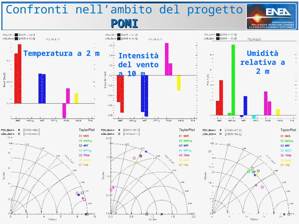
Confronti nell’ambito del progetto POMIPOMI
Temperatura a 2 m Intensità del vento a 10 m
Umidità relativa a 2
m
Confronti nell’ambito del progetto POMIPOMIATTIVITÀ DI VALIDAZIONE DEI CAMPI
METEOROLOGICI 2005
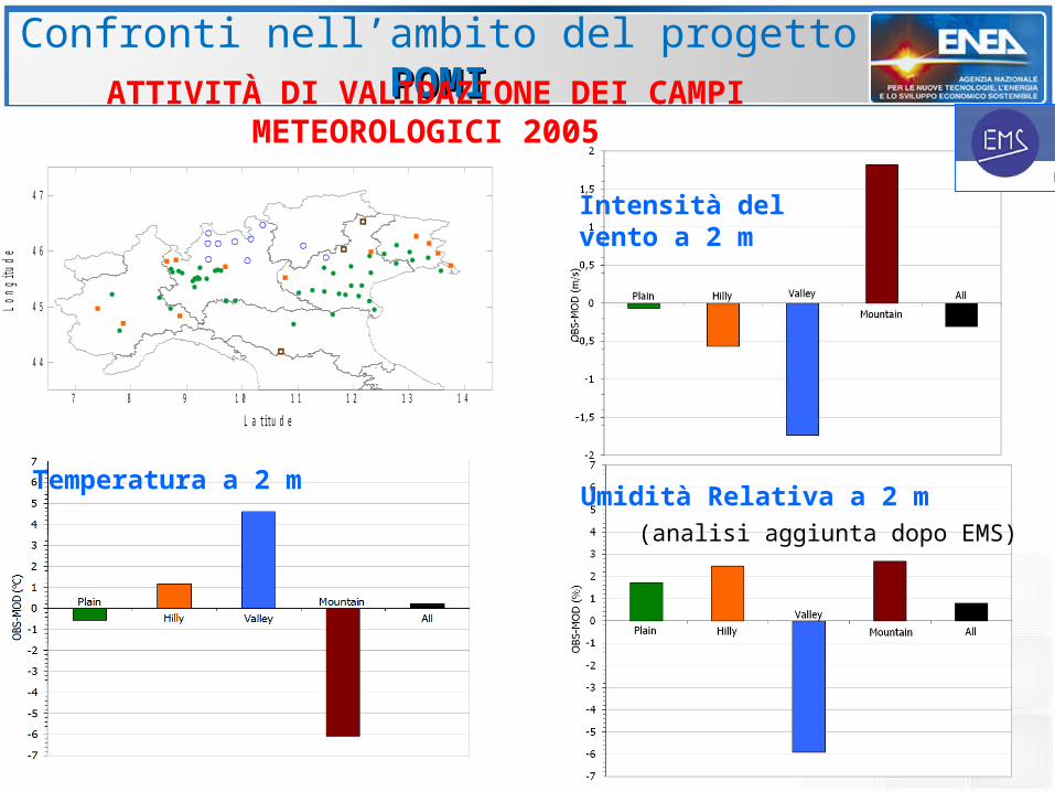
Confronti nell’ambito del progetto POMIPOMI
7 8 9 1 0 1 1 1 2 1 3 1 4
L a t i t u d e
4 4
4 5
4 6
4 7
Long
itude
Temperatura a 2 m
Intensità del vento a 2 m
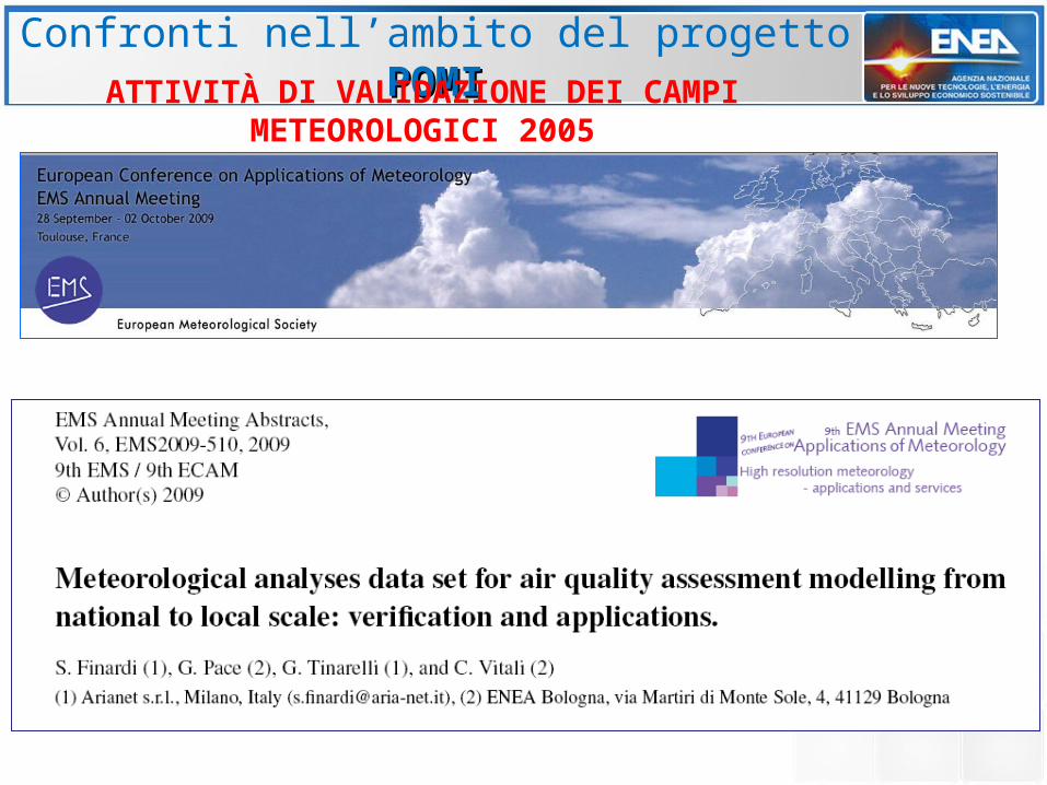
ATTIVITÀ DI VALIDAZIONE DEI CAMPI METEOROLOGICI 2005
Umidità Relativa a 2 m(analisi aggiunta dopo EMS)
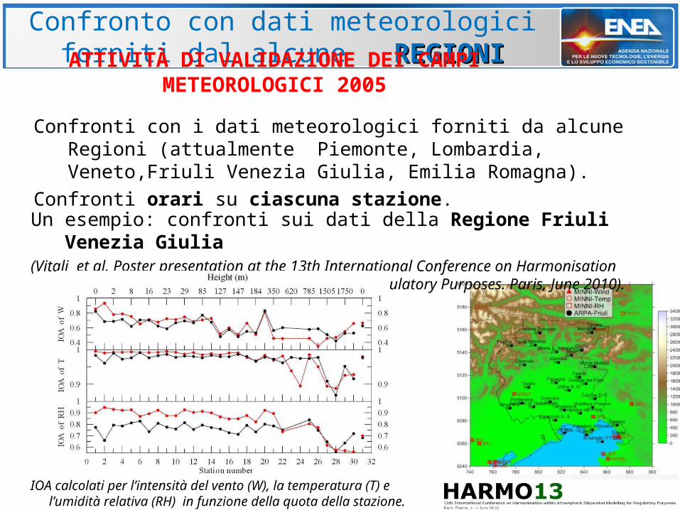
Confronti con i dati meteorologici forniti da alcune Regioni (attualmente Piemonte, Lombardia, Veneto,Friuli Venezia Giulia, Emilia Romagna).
Confronti orari su ciascuna stazione.
Confronto con dati meteorologici forniti dal alcune REGIONIREGIONIATTIVITÀ DI VALIDAZIONE DEI CAMPI METEOROLOGICI 2005
Un esempio: confronti sui dati della Regione Friuli Venezia Giulia
(Vitali et al. Poster presentation at the 13th International Conference on Harmonisation within Atmospheric Dispersion Modelling for Regulatory Purposes. Paris, June 2010).
IOA calcolati per l’intensità del vento (W), la temperatura (T) e l’umidità relativa (RH) in funzione della quota della
stazione. Nero:RAMS Rosso:LAPS
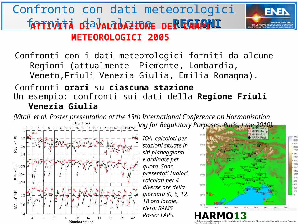
Confronti con i dati meteorologici forniti da alcune Regioni (attualmente Piemonte, Lombardia, Veneto,Friuli Venezia Giulia, Emilia Romagna).
Confronti orari su ciascuna stazione.
Confronto con dati meteorologici forniti dal alcune REGIONIREGIONIATTIVITÀ DI VALIDAZIONE DEI CAMPI METEOROLOGICI 2005
Un esempio: confronti sui dati della Regione Friuli Venezia Giulia
(Vitali et al. Poster presentation at the 13th International Conference on Harmonisation within Atmospheric Dispersion Modelling for Regulatory Purposes. Paris, June 2010).
IOA calcolati per stazioni situate in siti pianeggianti e ordinate per quota. Sono presentati i valori calcolati per 4 diverse ore della giornata (0, 6, 12, 18 ora locale). Nero: RAMS Rosso: LAPS.
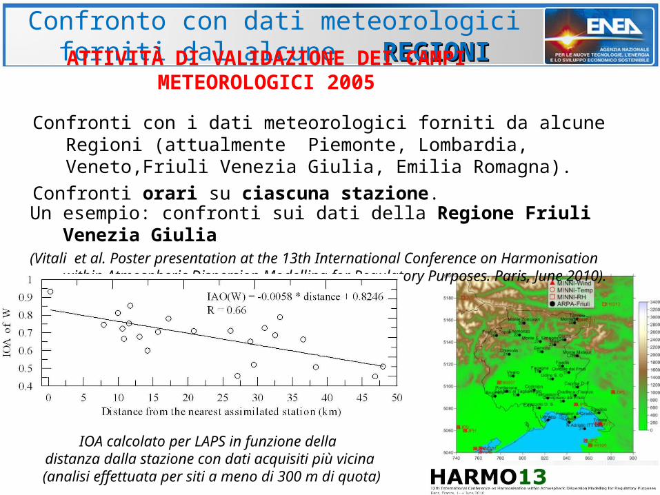
Confronti con i dati meteorologici forniti da alcune Regioni (attualmente Piemonte, Lombardia, Veneto,Friuli Venezia Giulia, Emilia Romagna).
Confronti orari su ciascuna stazione.
Confronto con dati meteorologici forniti dal alcune REGIONIREGIONIATTIVITÀ DI VALIDAZIONE DEI CAMPI METEOROLOGICI 2005
Un esempio: confronti sui dati della Regione Friuli Venezia Giulia
(Vitali et al. Poster presentation at the 13th International Conference on Harmonisation within Atmospheric Dispersion Modelling for Regulatory Purposes. Paris, June 2010).
IOA calcolato per LAPS in funzione della distanza dalla stazione con dati acquisiti più vicina (analisi effettuata per siti a meno di 300 m di quota)
celina
The comparison of RAMS and LAPS results with observations shows that: - LAPS provides a generally better description of meteorological fields in the coastal and inland plain area, which is the main target for air quality assessment; - it obtains better statistical indicators of model performance, for all the common meteorological variables. The temperature diurnal cycle is better reproduced by LAPS and, in particular, it corrects RAMS nocturnal overestimation. A relevant improvement is obtained for humidity, that is important for air quality applications because humidity influences PM and OH formation. The correction imposed by LAPS over RAMS wind speed is less clearly interpretable from statistical indicators, even if FB indicates the correction of RAMS overestimation, that is changed into a slight underestimation in LAPS results. This feature is quite relevant due to the influence of wind intensity on pollutants transport and dispersion.
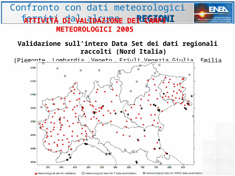
Validazione sull’intero Data Set dei dati regionali raccolti (Nord Italia)(Piemonte, Lombardia, Veneto, Friuli Venezia Giulia, Emilia Romagna).
Confronto con dati meteorologici forniti dal alcune REGIONIREGIONIATTIVITÀ DI VALIDAZIONE DEI CAMPI METEOROLOGICI 2005
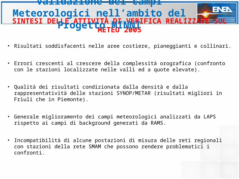
• Risultati soddisfacenti nelle aree costiere, pianeggianti e collinari.
• Errori crescenti al crescere della complessità orografica (confronto con le stazioni localizzate nelle valli ed a quote elevate).
• Qualità dei risultati condizionata dalla densità e dalla rappresentatività delle stazioni SYNOP/METAR (risultati migliori in Friuli che in Piemonte).
• Generale miglioramento dei campi meteorologici analizzati da LAPS rispetto ai campi di background generati da RAMS.
• Incompatibilità di alcune postazioni di misura delle reti regionali con stazioni della rete SMAM che possono rendere problematici i confronti.
SINTESI DELLE ATTIVITÀ DI VERIFICA REALIZZATE SUL METEO 2005
Validazione dei campi Meteorologici nell’ambito del
Progetto MINNI
celina
Validation results show a satisfactory description for all the considered meteorological variables over coastal and inland plains, which are the main target areas for air quality assessment and management in Italy. The model performance slightly deteriorates over mountain areas, especially as far as wind fields reconstruction is concerned. This shortcoming is mainly attributable to model resolution, which is insufficient to properly resolve Alpine valleys features and to reproduce sharp mountain or valley measured values.
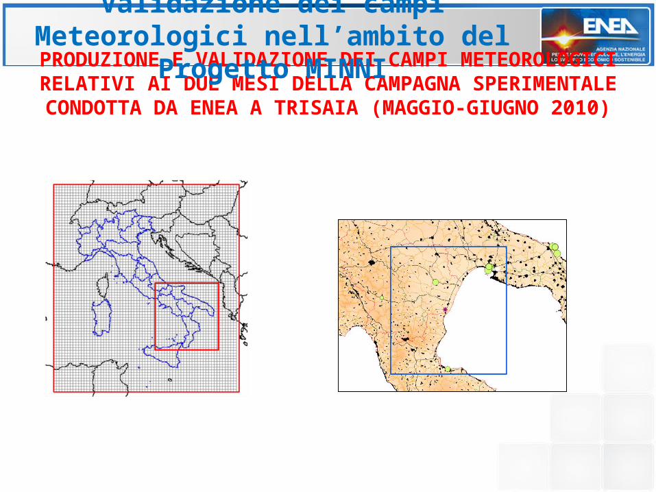
PRODUZIONE E VALIDAZIONE DEI CAMPI METEOROLOGICI RELATIVI AI DUE MESI DELLA
CAMPAGNA SPERIMENTALE CONDOTTA DA ENEA A TRISAIA (MAGGIO-GIUGNO 2010)
Validazione dei campi Meteorologici nell’ambito del
Progetto MINNI
PRODUZIONE E VALIDAZIONE DEI CAMPI METEOROLOGICI RELATIVI AI DUE MESI DELLA
CAMPAGNA SPERIMENTALE CONDOTTA DA ENEA A TRISAIA (MAGGIO-GIUGNO 2010)
Validazione dei campi Meteorologici nell’ambito del
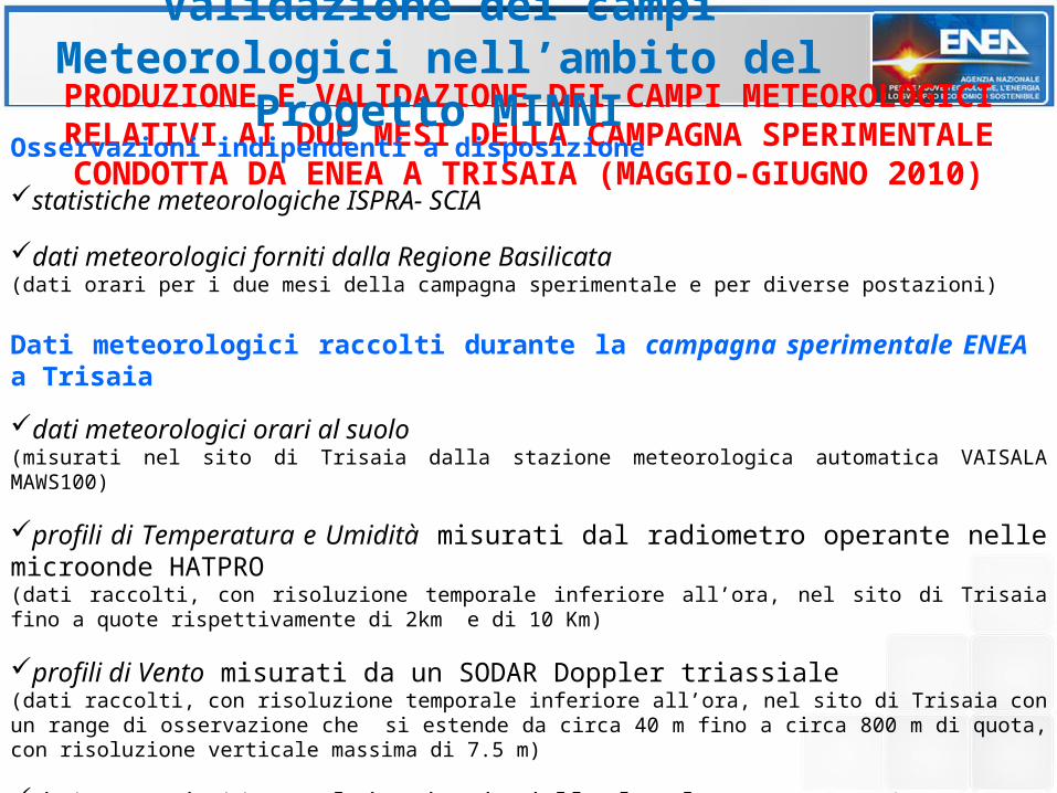
Progetto MINNIOsservazioni indipendenti a disposizione
statistiche meteorologiche ISPRA- SCIA
dati meteorologici forniti dalla Regione Basilicata (dati orari per i due mesi della campagna sperimentale e per diverse postazioni)
Dati meteorologici raccolti durante la campagna sperimentale ENEA a Trisaia
dati meteorologici orari al suolo (misurati nel sito di Trisaia dalla stazione meteorologica automatica VAISALA MAWS100)
profili di Temperatura e Umidità misurati dal radiometro operante nelle microonde HATPRO (dati raccolti, con risoluzione temporale inferiore all’ora, nel sito di Trisaia fino a quote rispettivamente di 2km e di 10 Km)
profili di Vento misurati da un SODAR Doppler triassiale (dati raccolti, con risoluzione temporale inferiore all’ora, nel sito di Trisaia con un range di osservazione che si estende da circa 40 m fino a circa 800 m di quota, con risoluzione verticale massima di 7.5 m)
dati meteorologici raccolti a bordo dell’ultraleggero ENDURO_KIT (12 voli effettuati durante la campagna sperimentale ENEA, nell’ambito del progetto EUFAR, http://www.eufar.net/)
ATTIVITÀ DI VALIDAZIONE IN CORSO E PREVISTE NEL PROSSIMO FUTURO
Validazione dei campi Meteorologici nell’ambito del
Progetto MINNI
Paper sulla Validazione dei campi meteorologici MINNI 2005
Validazione sui dati delle Regioni del Nord Italia dei
campi meteorologici MINNI 2003 e 2007
Paper(s) sulla Validazione deicampi meteorologici MINNI a Trisaia
(maggio-giugno 2010)
RisultatiRisultati
Costruzione di una base dati meteorologica
per il supporto delle analisi di qualità dell’aria a livello nazionale e macroregionale
comprensiva di 4 anni di dati a risoluzione 20x20 e 4x4 km
(utilizzato con risultati positivi all’interno del progetto MINNI e da altri soggetti sia istituzionali che privati)
Soggetti che hanno utilizzato la base dati meteorologica Soggetti che hanno utilizzato la base dati meteorologica MINNIMINNI
Regione Piemonte, Provincia Torino, Regione Veneto-ARPAV, ARPA Valle d’Aosta, ARPA Friuli Venezia Giulia, ARPA Lazio, ARPA Puglia, APPA Bolzano, Magistrato alle Acque di Venezia, NOMISMA, CIPA (SR), SPEA-autostrade, AIB e società di consulenza per studi di
impatto ambientale (URS, Dappolonia, PROTECO, TECNIC)
CONSIDERAZIONI CONCLUSIVE
Campi Meteorologici nell’ambito
del Progetto MINNI