Productivity Dynamics in Manufacturing Plants (Brookings Papers ...
81
MARTIN NEIL BAILY University of Maryland CHARLES HULTEN Universityof Maryland DAVID CAMPBELL Universityof Maryland Productivity Dynamics in Malnufcacturing Plants MUCH OF THE TRADITIONAL analysis of productivity growth in manu- facturing industries has been based explicitly or implicitly on a model in which identical, perfectly competitive plants respond in the same way to forces that strike the industry as a whole. The estimates of growth obtained with this frameworkare then used as the basis for discussions of policy concerning capital accumulation,research and development, trade, or other issues. This contrastsmarkedly with the literature of industrial organization in which perfectcompetition is seen as an unusual market structure andin which the differences amongfirms are examined in detail. The models of oligopoly that are the staple of the industrial organization literature are then used to examine antitrust policy. This research is being funded by the National ScienceFoundation (SES-9108976) and theCenter for Economic Progress andEmployment of the Brookings Institution withgrants fromthe FordFoundation and manycorporate sponsors. The authors would like to thank Robert McGuckin, MikeCohen, TimDunne, Mark Doms, Eric Bartelsman, Josh Haimson, Steve Olley, Hal Van Gieson, John Haltiwanger, Zvi Griliches,and participants in the Brookings panel on microeconomics for many helpfulconversations. We also appreciate the help of Robert Bechtoldand othermembers of the staff at the Center for Economic Studies at the Bureau of the Census(CES). Valuable comments on this workwere made in seminars at the NBER Summer Institute, at the Boardof Governors of the Federal Reserve in Washington, D.C., andat the University of Chicago. Martin Baily andCharles Hulten, Research Associates of the National Bureau of Economic Research, are affiliated with the Brookings Institution and the American Enterprise Institute respectively. Martin Baily andDavidCampbell are SpecialSwornEmployees of CES. 187
Transcript of Productivity Dynamics in Manufacturing Plants (Brookings Papers ...

MARTIN NEIL BAILY University of Maryland
CHARLES HULTEN University of Maryland
DAVID CAMPBELL University of Maryland
Productivity Dynamics in Malnufcacturing Plants
MUCH OF THE TRADITIONAL analysis of productivity growth in manu- facturing industries has been based explicitly or implicitly on a model in which identical, perfectly competitive plants respond in the same way to forces that strike the industry as a whole. The estimates of growth obtained with this framework are then used as the basis for discussions of policy concerning capital accumulation, research and development, trade, or other issues. This contrasts markedly with the literature of industrial organization in which perfect competition is seen as an unusual market structure and in which the differences among firms are examined in detail. The models of oligopoly that are the staple of the industrial organization literature are then used to examine antitrust policy.
This research is being funded by the National Science Foundation (SES-9108976) and the Center for Economic Progress and Employment of the Brookings Institution with grants from the Ford Foundation and many corporate sponsors. The authors would like to thank Robert McGuckin, Mike Cohen, Tim Dunne, Mark Doms, Eric Bartelsman, Josh Haimson, Steve Olley, Hal Van Gieson, John Haltiwanger, Zvi Griliches, and participants in the Brookings panel on microeconomics for many helpful conversations. We also appreciate the help of Robert Bechtold and other members of the staff at the Center for Economic Studies at the Bureau of the Census (CES). Valuable comments on this work were made in seminars at the NBER Summer Institute, at the Board of Governors of the Federal Reserve in Washington, D.C., and at the University of Chicago. Martin Baily and Charles Hulten, Research Associates of the National Bureau of Economic Research, are affiliated with the Brookings Institution and the American Enterprise Institute respectively. Martin Baily and David Campbell are Special Sworn Employees of CES.
187

188 Brookings Papers: Microeconomics 1992
In the past few years there has been greatly increased interest in improving the microeconomics of productivity analysis and in recon- ciling it with models of the organization of industry. i This paper is an attempt to improve the empirical basis for this work.2 We will explore the heterogeneity among plants to see how individual plants move within an industry, which plants account for most of the productivity growth, and how important entry and exit are to industry growth. In developing our findings, we will be using the Longitudinal Research Database (LRD) prepared by the Center for Economic Studies of the Bureau of the Census. As we have examined this data, we have been impressed by the diversity among plants and among industries. Some industries in our sample have achieved huge improvements in productivity; in others productivity has fallen sharply. There are high-productivity en- trants and low-productivity entrants, high-productivity exiters and low- productivity exiters, plants that move up rapidly in the productivity distribution and plants that move down rapidly. Many plants stay put in the distribution. Both in level of and rate of change in productivity, plants manifest significant differences.3 The aggregate productivity per- formance of the manufacturing sector reflects the average of diverse economic outcomes at the plant level. Jacques Mairesse and Zvi Gril- iches put the issue forcefully: "The simple production function model, even when augmented by additional variables and further nonlinear terms, is at best just an approximation to a much more complex and changing reality at the firm, product, and factory floor level."4
In the face of this complexity, we proceed with a minimum amount of structure. Our purpose is not to test a single model, but to sort out
1. Romer (1990) and Hall (1988, 1990) have built on work by Schumpeter (1936, first published 1911), Griliches and Ringstad (1971), Griliches (1979), Nelson and Winter (1978, 1982), and Scherer (1984). Nelson and Winter, in particular, stress that models of aggregate economic growth and productivity increase must be consistent with the wide diversity of plant-level performance that is observed in the data.
2. We recognize the theoretical and empirical contributions of Jovanovic (1982), Gril- iches and Mairesse (1983), and others in exploring industry dynamics. We believe, however, that there is a need to explore further the empirical basis for productivity dynamics.
3. Some of the implications of the plant-level heterogeneity have already been docu- mented. See Dhrymes (1990); and Olley and Pakes (1990). For a recent and somewhat parallel study to ours, see Bartelsman and Dhrymes (1992). Davis and Haltiwanger (1991) also examined plant-level heterogeneity from the wage and employment side.
4. Mairesse and Griliches (1990, p. 221).

Martin Neil Baily, Charles Hulten, and David Campbell 189
alternative views about the appropriate model for explaining the dis- tribution of productivity and its evolution over time.
A Preview of Results and Their Relevance for Policy
We look first at the contribution of different groups of plants to industry productivity growth. Two interesting findings emerge. First, entry and exit play only a very small role in industry growth over five- year periods. Second, the increasing output shares in high-productivity plants and the decreasing shares of output in low-productivity plants are very important to the growth of manufacturing productivity.
Do the plants with high or low productivity remain in the same relative position, or is there a reshuffling of plants over time? We will look next at the question of persistence. The report of the MIT com- mission suggests that plants at the top of the productivity distribution rest on their laurels and lose their competitive advantage.5 We conclude that being at the top often conveys advantages that allow the leading plants to stay there. Our finding is consistent with the idea of well- managed plants that are able to stay on top for long periods.
The manufacturing sector experienced a resurgence of productivity growth in the 1980s, and so we look for changes in the productivity distribution or the pattern of entry and exit that might reflect this shift. We found no dramatic differences over time in the pattern of plant dynamics that correspond to the periods of slow and rapid productivity growth, but there were signs of greater mobility among plants in the 1980s. The degree of persistence has declined over time.
There is great interest at present in the distribution of wages and the sources of wage differences. We examine one aspect of this: the relation between plant-level productivity and plant-level wages. The two are strongly correlated, and there are two possible explanations. One is that some plants hire high-skill workers and pay high wages. An alternative reason is that workers in high-productivity plants are able to demand higher wages.
We find strong firm effects in our data. Plants that are part of high- productivity firms will also have higher productivity. Plants in firms
5. Dertouzos, Lester, and Solow (1989).

190 Brookings Papers: Microeconomics 1992
where there is rapid productivity growth will grow more rapidly. There may be common characteristics to plants in the same firm, or there may be spillovers in R&D or product design or management methods that help plants in the same firm.
With regard to policy analysis, the role of the economist is often to warn against the adverse effects of proposed policies. Pointing to the frequency with which plants close, some observers argue that U.S. manufacturing is in trouble and needs policies to protect it. Policies to reduce such closings have been proposed in order to prevent "dein- dustrialization." But plant closings are indicative of both success and failure. The frequency of plant closings is very high (even of high- productivity plants) within highly successful and growing industries. While we recognize the costliness of plant closings, it is important to decide whether policies to prevent industrial restructuring could inhibit the evolution of successful industries.
In the area of antitrust, analysis of plant-level dynamics can help us understand the life cycle of plants: they enter an industry, grow, decline, and exit. The nature and timing of this cycle will have implications for market concentration over time and for firm-level profitability. An im- portant contribution to productivity growth in manufacturing comes from increases in the share of output produced in the above-average productivity plants. It is often remarked that antitrust policy should not discriminate against firms that are large because they are better. We reinforce that conclusion. Indeed, it is important to allow the better plants to get bigger.
Strong firm effects may have implications for antitrust policies to- ward takeovers. Our results are consistent with the hypothesis that a plant that joins a high-productivity firm will receive spillover benefits that will raise its own productivity. Further work, however, is needed to verify that the strong firm effects are the result of spillovers.
Productivity Distribution and Dynamics: The Basic Theory
We will use a neoclassical production function for which Qi, is the real gross output of the ith plant in year t, and Kit, Lit, and Mi, are capital, labor, and intermediate inputs, respectively. This last input

Martin Neil Baily, Charles Hulten, and David Campbell 191
includes energy and an estimate of purchased services, all accounted for separately:
(1) Qit = F(Kit, Lit, Mit).
The production function provides the basis for computing the relative total factor productivity (TFP) of each plant. We have used two alter- native ways of calculating relative TFP for the plants in our sample.
The first way is similar to the approach used by Olley and Pakes and by Bartelsman and Dhrymes.6 It can be expressed
(2) lnTFPit = lnQit - xKlnKit - cxLlnLit - oxMlnMit.
The level of productivity in an industry in year t is then represented by the following index:
(3) lnTFPt = E OitlnTFPit,
where Oit is the share of the ith plant in industry output in current dollars. The growth of industry TFP over the period t - T to t is then
(4) AInTFPt = lnTFPt - lnTFPt,T.
The industry growth rates calculated in this way agree reasonably well with the growth rates calculated by Wayne Gray from aggregate industry data. 7
We also have used the approach suggested by Christensen, Cum- mings, and Jorgenson: relative TFP is calculated by relating the devia- tion of plant output from the industry mean to the deviations of the factor inputs from the industry means.8
For both of the alternative approaches to relative productivity, we estimate the factor elasticities using cost shares, which do not add to unity, thus avoiding the assumption of constant returns to scale. The
6. Olley and Pakes (1990); and Bartelsman and Dhrymes (1992). 7. Gray's file of four-digit manufacturing productivity estimates is available through
the National Bureau of Economic Research. 8. See Christensen, Cummings, and Jorgenson (1981). The specification in this case
is
lnTFPi= lnQi-InQ ctk[lnKi-lnK] - cL[lnLi-lnL] -(xM[lnMi-FniM]],
where Q, K, L, and M are the industry average values of output and factor inputs. The relative TFP index is adjusted to have mean zero for each industry.

192 Brookings Papers: Microeconomics 1992
capital share is based on the rental cost of capital; equipment, structures, and inventory rental rates are taken from the Bureau of Labor Statistics.9 When we calculate TFP for industry growth analysis, we use the spec- ification shown in equation 4, and we take the factor elasticities to be the industry average factor income shares, averaged again over the beginning and ending year of the period of growth. When we focus on the relative productivities of plants within an industry within a single year, we use the approach by Christensen, Cummings, and Jorgenson. We take the factor elasticities for a given plant as the average of the plant's factor cost shares and the industry shares. This method is better for giving the relative productivity of a given plant in a single year.
There is an important property of the relative productivity rankings: they do not depend upon the output deflator. For a given year a dollar is a dollar, and output is measured in the same units in all plants.10 And this virtue even extends to some intertemporal comparisons. For example, we can see how plants move in the rankings from one period to the next without introducing errors from the output deflator. The deflators are, of course, important to any calculation of productivity growth over time, for individual plants or for the industry.
Decomposition of Industry Productivity Growth
Using the relative productivity of each plant within its industry, we can rank the plants and order them from the highest relative productivity to the lowest in a particular year and divide the plants into quintiles. When we compare two time periods, we can see which plants have stayed in the quintile they started in, which have moved up, and which have moved down. We also account for the entry and exit of plants in our decomposition of industry productivity growth. With access to the Censuses of Manufactures we can determine, for the exits, whether a given plant has closed down or switched to another industry. For the
9. In order to assume that the cost shares reflect the factor elasticities in the production function, we do have to assume competition in factor markets.
10. Of course, plants within the same four-digit industry do produce different outputs. Plants that choose more profitable outputs are counted as having higher productivity in our analysis.

Martin Neil Baily, Charles Hulten, and David Campbell 193
entrants we can find the newly opened plants and the ones that have switched in from another industry. 1I
With this information we can decompose industry productivity growth into the contributions of the stayers, the entrants, and the exits. And we can further decompose the productivity growth of the stayers to see how much of overall growth is from the plants that moved up in the productivity distribution, from those that stayed on top, and so on. We now explain specifics of the decomposition.
Looking back at equation 3, we know that some of the plants op- erating in t will also have been operating in a prior year t-T. These plants are designated the "stayers" (the set S). Some of the plants operating in t will be plants that have entered between t -T and t (the set N). Some plants operating in the year t -T are no longer operating in t. They have exited the industry (the set X). The change in produc- tivity between t-T and t is then as follows:
AlnTFPt = (0tlnTFPjt - Oit TlnTFPjt,T) iES
(5) + Ot,lnTFPi,- E Oit-TlnTFPit-T) ieN ie-X
Productivity growth in the industry reflects the growth among the stayers, changes in output shares, and the effect of the entrants and exits. The net effect of the exits and entrants will reflect any differences in the levels of productivity between the groups and any differences in the output shares. The productivity growth among the stayers can be broken down in two ways. First, their contribution can come from improvements in each plant separately (holding output shares constant) and from changes in the output shares:
E (0tlnTFPjt - OitlTnTFPit-7) = E OitlTAlnTFPit iES iES
(6) + E (it - Oit-T) lnTFPit. iES
11. It is possible that a plant that we classify as a "death" is still operating, but not
194 Brookings Papers: Microeconomics 1992
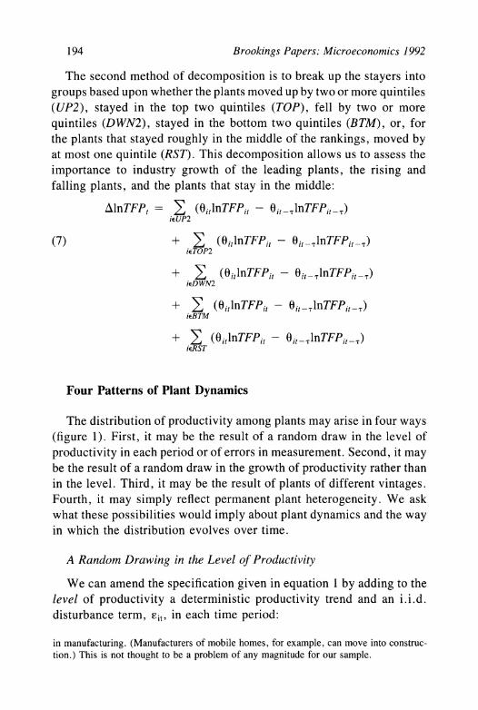
The second method of decomposition is to break up the stayers into groups based upon whether the plants moved up by two or more quintiles (UP2), stayed in the top two quintiles (TOP), fell by two or more quintiles (DWN2), stayed in the bottom two quintiles (BTM), or, for the plants that stayed roughly in the middle of the rankings, moved by at most one quintile (RST). This decomposition allows us to assess the importance to industry growth of the leading plants, the rising and falling plants, and the plants that stay in the middle:
AInTFPt = (0itInTFPit - Oit-TlnTFPjt_T) iEUP2
(7) + (0itlnTFPit- it-TlnTFPjt_T) iETOP2
+ E (0itlnTFPit -itOTlnTFPjt_T) ieDWN2
+ E (0itInTFPit- it-TlnTFPjt_T) ieBTM
+ E (0itInTFPit- it-TlnTFPjt_T) iERST
Four Patterns of Plant Dynamics
The distribution of productivity among plants may arise in four ways (figure 1). First, it may be the result of a random draw in the level of productivity in each period or of errors in measurement. Second, it may be the result of a random draw in the growth of productivity rather than in the level. Third, it may be the result of plants of different vintages. Fourth, it may simply reflect permanent plant heterogeneity. We ask what these possibilities would imply about plant dynamics and the way in which the distribution evolves over time.
A Random Drawing in the Level of Productivity
We can amend the specification given in equation 1 by adding to the level of productivity a deterministic productivity trend and an i.i.d. disturbance term, F-it, in each time period:
in manufacturing. (Manufacturers of mobile homes, for example, can move into construc- tion.) This is not thought to be a problem of any magnitude for our sample.

Martin Neil Baily, Charles Hulten, and David Campbell 195
(8) Qit = F(Kit, Lit, Mit) et?Ei.
Under this assumption relative productivity will be uncorrelated from period to period. There will be no persistence in the productivity dis- tribution, and the TFP of a plant in one period will have no predictive power for the TFP in another period. Plants that look productive in one period will have received a good random draw or will look good because of errors in the data. This is the case where the industry consists of identical plants that differ in observed data only because of the random shocks or data errors.
Figure IA illustrates this case. An index of plant-level TFP is on the vertical axis (log scale), and time is on the horizontal axis. In any sample year the plants in the industry are spread out on a vertical line. The bell-shaped curve indicates the frequency distribution of plants along the line. The straight line gives the common path of trend pro- ductivity growth (slope ,3). In figure IA the plant that is shown with above average productivity at point A in time t, is as likely to be at B, above the mean, as at C, below the mean, in time t2.
The assumption of an i.i.d. error is obviously a strong one, but in general, if the relative productivities of individual plants move around rapidly from period to period, and the persistence in relative produc- tivity declines as the period is increased, then this will show that random shocks or data errors are major determinants of the distribution of productivity across plants.
Random Productivity Growth
In equation 8 it is assumed that there is a random shock to the level of productivity. An alternative specification would be that there is a random shock to the growth of productivity:
(9) AlnTFPit = 3 + Eit,
where again ,it is an i.i.d. disturbance. This case is illustrated in figure lB. Plants that are high in the productivity distribution in time t, will remain high on an expected value basis. A plant that starts with relative productivity shown at point A will have an expected relative productivity at B at time t2. But plants will be as likely to decline as to rise, so the overall productivity distribution will show increasing variance over time.

196 Brookings Papers: Microeconomics 1992
Figure 1. Alternate Views of Distribution of Productivity
A. PRODUCTIVITY DISTRIBUTION AS B. RANDOM GROWTH IN
A RANDOM SHOCK PRODUCTIVITY
Log TFP Log TFP
B~~~~~~~~~ A~~~~~~~~
tI t2 t ti t2 t3
Time Time
C. PRODUCTIVITY IN THE VINTAGE D. PRODUCTIVITY WITH
CAPITAL MODEL HETEROGENEOUS PLANTS
Log TFP ~~~~~Log TEPB
A
A A" Log TFP
C t C Exit D Exit
(I t- t3 tI t' t3
Time Time

Martin Neil Baily, Charles Hulten, and David Campbell 197
This framework suggests that the floor to productivity will be very important. If there is some minimum level of relative productivity, shown in figure lB by the dashed line, then this will truncate the productivity distribution at the bottom. The exit of low-productivity plants will become an important element in overall productivity per- formance. We would also expect that the gap between the plants in, say, the top quintile and the plants in the next quintile will gradually widen over time.
The Vintage Capital Model
This model assumes that when a plant is built it embodies a particular vintage of technology. Therefore, the production function includes a measure of the vintage of the plant, vi,:
(10) Qit = F(Ki,, Lit, Mit, vit)
The age of the plant is an obvious way to measure vintage. Under the assumptions of the vintage model, the most productive plants in a given period are earning a large quasi rent. Over time these plants will fall back in the productivity distribution until they can no longer earn pos- itive quasi rents, and they are then closed. Figure IC illustrates the case of vintage capital. At time t1 there are four active plant vintages shown at A, B, C, and D. The most productive plant/vintage is at point A and the least productive is at D. After one period there has been entry of a new vintage at point E. This is the new high-productivity plant. Plant A has remained at the same level of productivity and is now at A', in the second spot. Plants B and C have moved to B' and C', and plant D has exited the industry.
In practice, this vintage model would be superimposed on the random shocks case. There are certainly some errors in the data. Nevertheless, if the vintage model has power to explain the distribution of plant-level productivity, the relative productivities of surviving plants will be de- clining over time. The relative productivity of a plant in one period will equal its relative productivity in the previous period minus a down- ward shift effect (plus an error term). For plants that are above the mean, the decline of relative productivity will move them toward the mean. This also was the case in the random shocks model (regression toward the mean). Plants below the mean, however, will be moving

198 Brookings Papers: Microeconomics 1992
away from the mean, and plants at the bottom of the distribution will exit. Any negative trend in relative productivity can be identified even in the presence of random errors or shocks. The exit of low-productivity plants and the entry of high-productivity plants will be important for overall productivity growth.
Although the basic idea of vintage technology is plausible, the iden- tification of plant age (or indeed of any characteristic of a plant) with technology vintage is questionable. There are many old plants in the LRD that have been re-equipped. If we find that this model does not fit the data very well, this does not refute the hypothesis that new equipment embodies the most advanced technology. If plant age turns out to be unimportant, it may be preferable to return to the standard neoclassical function, assuming that technological change is capital augmenting and is being correctly captured in the capital price deflators. This assumption can be tested by seeing if high levels of recent in- vestment have an effect on productivity.
Plant Fixed Effects
The distribution of productivity at a point in time may be the re- flection of permanent plant heterogeneity, or at least of heterogeneity that is long term relative to the time periods that we will consider. Later we will discuss factors that might lead to such long-term plant differ- ences. The production function in this case is
( 1 ) Qit = F(Kitg Lit, Mit, vi),
where vi represents an arbitrary fixed effect that does not change over time and is not associated with the vintage of the plant. This framework assumes that plants will differ not only in their factor intensities but also in the technologies that they use. In this case we would expect to see several signs of strong persistence in relative plant productivities. Relative productivity in one year will be a good predictor of relative productivity in subsequent years. Allowing for plant fixed effects in time-series cross-sectional production or productivity estimates will provide much of the explanation of the productivity distribution.
Figure ID illustrates this case. Each plant is on its own parallel growth path. A plant that is at point A (at a point, say, 10 percent above the average in one period, tl) can be expected to be at point B (still 10

Martin Neil Baily, Charles Hulten, and David Campbell 199
percent above the average in the subsequent period, t2). The distribution of random error is indicated by the small bell-shaped curves.
As before, this case of persistent heterogeneity is an extreme one. Data errors will lead to less than complete persistence even if there is true permanent heterogeneity. Nevertheless, it is possible within the LRD sample to assess the extent to which high- or low-productivity plants tend to remain in their relative positions.
Plant Productivity Effects
The last case, the case in which plant productivity effects persist, turns out to be an important feature in the results. We explore this case more fully now and look at some of the variations that have been suggested on this theme.
Returns to Scale and Utilization Effects
The simple production function given in equation 1 was assumed to have constant returns to scale. But this condition may not hold, par- ticularly at the plant level. The empirical literature has suggested that there may be some increasing returns at this level.12 One possible ex- planation of the distribution of plant-level productivities is that different plants are operating at different scales. Scale varies slowly over time. If scale is an important determinant of productivity, this will give rise to persistence in the productivity distribution. If big plants are high in the distribution, then their size will help them stay at the top.
Returns to scale in the production function, as we have been de- scribing it, are an attribute of the production frontier. But if there are variations in utilization that result from variations in aggregate demand, then we would expect to see short-run declines in productivity that reflect labor hoarding, overhead labor, or one of the other reasons that are given for the cyclical productivity puzzle. In particular, one of our census years is 1982, a deep recession year.
If all plants in a given industry are affected in the same way by
12. See, for example, Griliches and Ringstad (1971). Hall (1988) has stressed increasing returns based on results from industry data.

200 Brookings Papers: Microeconomics 1992
recession, or if differences across plants are purely random, then the distribution of productivities across plants may not be changed that much when we compare 1982 with, say, 1977 or 1987. That may not be true, however. The productivity distribution may change in 1982 as a result of the recession. That is not easy for us to model explicitly because there are no direct measures of capital or labor utilization. In this paper we will simply explore the ways in which our results change in 1982. Does the degree of persistence change? Do entry and exit play different roles?
Differences in Managerial Ability
A common-sense explanation of the distribution of productivities across plants or firms is that some are better managed than others. Good plant managers run high-productivity plants, and good firm managers have many high-productivity plants. Persistent differences in manage- ment ability have been suggested as an explanation for persistence in relative productivity and for the importance of the plant fixed effects that we have described earlier."3 We would interpret a finding of per- sistence in relative productivity as being consistent with managerial differences as a source of the distribution. Many people have studied differences in managerial ability. We will review some of the findings and discuss their quite different implications.
Robert Lucas has proposed a model in which some people are en- dowed with greater managerial skills than are others,14 but there are diminishing returns to this skill as it is applied to larger and larger plants. An implication of this model is that there is an optimal (output- maximizing) distribution of firm sizes. This is implied by the distri- bution of managerial abilities. Lucas assumes factor prices are equal across plants. Therefore, plant output is proportional to plant employ- ment in the plant. In Lucas's model, average labor productivity is the same in all plants. The differences in skill among managers have all been absorbed in size.'5
13. See Abernathy, Clark, and Kantrow (1983); Hayes, Wheelwright, and Clark (1988); Caves and Barton (1990); and Dertouzos, Lester, and Solow (1989).
14. Lucas (1978). 15. Intuitively this result may be surprising since the optimal allocation of managers
involves equating marginal benefits not average benefits. The constant elasticity (Cobb-

Martin Neil Baily, Charles Hulten, and David Campbell 201
A kind of Parkinson's law is at work: the greater the skill of the manager, the larger the plant he or she manages. But it is still the case that able managers will earn higher returns than will poor managers. The returns will be proportional to the size of the plant. The Lucas specification allows a simple estimation of the parameters of the pro- duction and the managerial functions. With a Cobb-Douglas production function, the model predicts decreasing returns to scale. The diminish- ing returns measure the effects of the loss of productivity resulting from a given manager being spread too thin. A finding that size has a negative effect on productivity would be consistent, therefore, with the Lucas model.
The Lucas model postulates an equilibrium distribution of managerial abilities at all times. But information about managerial abilities is im- perfect, and so it is unlikely that this equilibrium will always prevail. Boyan Jovanovic has developed an important dynamic model of plant productivity that is similar to the Lucas framework.16 In the Jovanovic model, firm managers also have an intrinsic ability level that does not change over time. Whereas in the Lucas model, managers are assigned optimally to the plant that best suits their abilities, in the Jovanovic model, managers are entrepreneurs who start out small and then learn about their abilities over time, subject to random productivity shocks. On the basis of what happens to them over time (they observe a series of shocks), the firms decide whether to expand, contract, or go out of business. 17
Both the Lucas and the Jovanovic models are based on fully optimal responses by plant managers. But the view of Kim Clark, the MIT Commission, and indeed Caves and Barton is that managers do not
Douglas) assumptions of the model lead to the condition that average productivities end up the same.
16. Jovanovic (1982). 17. One empirical implication of the Jovanovic model is that large firms will have a
lower probability of exiting than small firms will have. This prediction has been supported for the LRD by Dunne, Roberts, and Samuelson (1988). Another empirical prediction of the Jovanovic model is that, since firm ability is fixed, observations about size in some early period should convey information about size in later periods, even conditional upon size information in intermediate periods. This prediction has been challenged in the active learning model of Ericson and Pakes (1989). They assume that firms are able to invest in order to improve their ability parameter. Ericson and Pakes predict that the information about ability that is contained in early periods will gradually erode.

202 Brookings Papers: Microeconomics 1992
always perform up to the limit of their abilities.18 Consider then the innovative remnant model in which managers slack off over time and then are forced to change in order to survive.19 In this model plants move down in the productivity distribution in a way that is similar to the vintage model. This decline is not only the result of technological obsolescence. It also is the result of nonmaximizing behavior by man- agers. These managers do not change work arrangements or bother to innovate as long as the plant is performing satisfactorily. Once the plant has fallen to the bottom of the productivity distribution, the managers change and the plant then moves up to the top of the distribution again. Predictions in this model about plant dynamics are similar to those of the vintage model, except that we would expect to see a cycling of plants in the productivity distribution, with plants that have been at the bottom of the distribution moving up to the top.
In addition to differences in managerial quality, there is another reason why some plants might remain above or below average in pro- ductivity over a long period of time: differences in the quality of their workforces.
Differences in Workforce Quality
Our estimates of productivity already include one adjustment for differences in the quality of workers. We distinguish between produc- tion and nonproduction workers. The labor input is computed as pro- duction-worker hours plus a quality-adjusted estimate of nonproduction hours. The adjustment is made using the relative earnings of nonpro- duction employees (with the calculations made separately for each plant). Nonproduction workers on average have higher wages than production workers have. The wage difference (one that has grown over time) is attributed to skill differences. Therefore, one source of productivity increase in manufacturing-namely, the shift in the composition of the workforce toward higher skilled nonproduction workers-is being ad-
18. See Abernathy, Clark, and Kantrow (1983); Hayes, Wheelwright, and Clark (1988); Caves and Barton (1990); and Dertouzos, Lester, and Solow (1989).
19. We owe our interest in this model to Nelson and Winter (1978, 1982). Richard Nelson has indicated to us that the behavior of manufacturing plants in practice is more complex than we describe it. In his judgment our depiction of the cycling of plants is oversimplified. We will simply describe this case as the "innovative remnant" model.

Martin Neil Baily, Charles Hulten, and David Campbell 203
justed out of our analysis. We will show slower productivity growth than if productivity were calculated simply with an estimate of hours worked.
Consider now the effect of differences in the quality of production workers. Assume that there is an index qL of the average quality of the workforce in a given plant. The true production function for plant i would be
(12) Qi=F[Ki, Mi, (LiqjL)] ei,
where Fi is the distribution of productivity across plants, and the time subscript has been dropped. Suppose that the quality of individual work- ers is fully or partially reflected in the relative wage each is paid. In this case
(13) qi= Wi7.
We will obtain valid estimates of the effect of the relative wage on productivity, provided the relative wage paid is exogenous to the plant:
(14) lnTFPi = UL'YlnWi + Ei.
The coefficient on the wage in a TFP regression will identify the pa- rameter y, reflecting the relation between wage and quality. This re- lation could be the result of differences in skill levels. It also could be the effect of higher wages in raising work effort, as described by the efficiency wage theorists.
If the labor market is competitive-that is, if plants can select all the workers they want at a given level of quality-then market equi- librium will ensure that y is equal to unity. Any coefficient other than unity will lead plants to adjust either quality or quantity. In this case the wage should enter the productivity relation with the same coefficient as labor input.
Now assume an alternative framework. The workers are all identical, and there is no difference in work effort across plants. Workers, how- ever, are able to bargain for high wages in plants with high productivity. The wage itself will depend upon the distribution of productivity across plants. This can be expressed
(15) lnWi = constant + 86i + p,i

204 Brookings Papers: Microeconomics 1992
where pi is a disturbance term. Substituting this expression into the production function (with qL now equal to unity) gives the following:
1 (16) lnTFPi - lnWi + pi.
6
This case will also show the wage as being correlated with productivity. The true causation, however, is going the other way: productivity is causing the wage rather than the other way around.20
The strong correlation between the wage that a plant pays and the plant's productivity cannot simply be taken as a skill indicator. To study the link between wages and productivity, we introduce exogenous vari- ables that are correlated with the wage and then use two-stage estimates of the impact of wages on productivity and the impact of productivity on wages. We draw on the work of Tim Dunne and Mark J. Roberts.21 They have developed a two-stage model of plant closings where wages affect the probability of closing and vice versa. They use indicators of local labor market conditions that are exogenous to plant-level decisions and explain about 40 percent of plant wage variations.
The Data
The Longitudinal Research Database has been developed by the Cen- ter for Economic Studies at the Census Bureau. It contains information from manufacturing establishments from the census years 1963, 1967, 1972, 1977, 1982, and 1987 and from the Annual Survey of Manufac- turers (ASM) establishments from 1972 to 1988. Making use of work at the center on the linkage of plant observations (by Tim Dunne, John Haltiwanger, Steve Davis, Scott Schuh, and others), we construct lon- gitudinal histories for each of the plants in the panel. Data are available only between census years for ASM plants. There is information in the data set on shipments and materials by detailed (seven-digit) product code; inventories, employment, wages, salaries, and fringe benefits for all workers and for production workers; energy use and cost of contract
20. In calculating TFP we have assumed competitive factor markets. If this assumption is violated, there may be some bias introduced into our TFP calculations.
21. Dunne and Roberts (1990).

Martin Neil Baily, Charles Hulten, and David Campbell 205
work; and investment, value of investment, book value of capital (struc- tures and equipment), and capital rentals. There is information on the ownership of the plant and whether it is part of a multiplant firm. There is no plant-level information on the purchases of services, except en- ergy. We use estimates of the ratio of materials purchased to purchased services made at the two-digit level by the Bureau of Labor Statistics to provide a crude correction for the increase in purchased services in manufacturing. There is geographic information on each plant.22
In the LRD there are difficulties with following plants over time (the linkage problem), and there are missing and nonsensical values that can create outliers large enough to throw off a whole regression or summary table. Plants that have relative productivity outside of a range plus and minus two of the industry mean have been considered "bad data." (Productivity is measured in logs so this corresponds to plants plus and minus 200 percent of the average.) They are primarily plants that are starting up or closing down, or they may be plants where the data have been entered incorrectly on the census form. Several people have warned us of the dangers of excluding outliers, and we have worked at length to minimize the number of plants involved. At this point our exclusions involve only a few plants, and we have checked these out on an individual basis. We were concerned that leaving these plants in the sample would generate considerable distortion, and we hope that leaving them out does not introduce a bias.
We have carried out our analysis in two stages. We experimented first with data for five four-digit industries: motor vehicle assembly, 3711; motor vehicle parts, 3714; construction equipment, 3531; com- puting equipment, 3573; and ball and roller bearings, 3562. We have data on these industries for all years from 1972 to 1988 and for the earlier censuses. For these industries we constructed capital stock data
22. See McGuckin and Pascoe (1988) for a discussion of the data and current research on it. Many people have looked at productivity at the plant level using the LRD. Lichtenberg and Siegel (1987) examine the effect of changes in ownership on productivity in individual plants. Gort, Bahk, and Wall (1991) look at the productivity of new and old plants. Nguyen and Reznek (1991) look at the five industries and examine whether there was evidence of nonconstant returns to scale, both from Cobb-Douglas parameters and from separate pro- duction function estimates of small and large plants. Doms (1990) estimates vintage capital effects in the steel industry. Streitwieser (1991) looks at plant-level diversification. Ad- ditional references are given in McGuckin (1989). For similar work on Canadian data, see Baldwin and Gorecki (1990).

206 Brookings Papers: Microeconomics 1992
using annual investment data and an estimate of initial capital stock; we allocated a plant's book value of capital to investment over its prior existence.
The second stage of the research was to study 23 industries (including the original 5), but with data only for the census years 1963, 1967, 1972, 1977, 1982, and 1987. The 23 industries are listed in appendix table A-1. There are data reported for all plants in the census, but the information is far from complete. Some plants are classified as "ad- ministrative record cases," and for these plants all of the data except employment are imputed. We have excluded these plants. Then the plants that are omitted from the Annual Survey of Manufacturers are not asked to report the book value of their capital except in 1987. The book value in the LRD is imputed.
We have compared results using only the 5 industries with good capital data, to results using the 23 industries with only the ASM plants, and to results with all of the plants except administrative record cases. There are some differences in results, particularly going from 5 indus- tries to 23. But the changes in the capital data do not seem to make much difference. Using the 5-industry sample as a test case, we found little difference between results with the book value of capital and results using our carefully constructed capital series. Labor and materials both have much larger cost shares than does capital so that the impact of errors in the capital input is attenuated.
We decided to use the 23-industry data but excluded the plants with imputed data. This means that we have used the plants that are part of the Annual Survey of Manufacturers. The danger is that we understate the small entrants. But since we have compared the results with those including all but administrative record cases, a reasonable picture of the larger sample is provided. We chose the 23 industries to give a broad spectrum of manufacturing plants, selecting from those industries where most plants produce a single product. (The primary product specialization ratios for the chosen industries were all over 80 percent.)
In our discussion of the alternative models of productivity, we have stressed the tremendous heterogeneity among manufacturing plants, the importance of entry and exit, and the fact that plants can both rise and fall in the distribution of productivity. We ask now how this hetero- geneity affects industry productivity growth.

Martin Neil Baily, Charles Hulten, and David Campbell 207
Table 1. Decomposition of TFP Growth, Selected Periods Percentage increase over the period
Entry and Category Total Fixed shares Share effect exit
1972-77
All industries 7.17 5.04 2.12 0.01 Except 3573 4.62 2.80 1.92 -0.09 Except 3573 and 3711 0.89 -0.86 1.84 -0.09
1977-82
All industries 2.39 - 1.09 2.53 0.95 Except 3573 - 3.18 - 6.08 2.49 0.41 Except 3573 and 3711 -4.80 -8.79 3.41 0.59
1982-87
All 15.63 13.52 3.15 -1.05 Except 3573 8.98 7.16 2.82 - 1.00 Except 3573 and 3711 9.30 7.59 2.60 -0.89
Source: Authors' calculations.
The Results of the Decomposition of Productivity
Table 1 gives the results of the decompositions we described earlier
based on the 23 industries for the 1972-77, 1977-82, and 1982-87
periods. We give only the weighted averages in the text to avoid an
overdose of numbers, but we refer to results for individual industries.
The industry detail is given in appendix table A- 1. The industry-average
figure weights each industry by its share of nominal gross output, av-
eraged over the beginning and ending years of the period. As well as the average growth for all of the industries together, we
give the averages excluding computer equipment (3573) and the av-
erages excluding both 3573 and motor vehicle assembly (3711). We
are mimicking the way in which the consumer price index (CPI) is
reported as "all items" and then "all items less energy" or "all items
less food and energy." The computer industry is singled out for special
treatment. Productivity growth in this industry is so large, captured by the quality-adjusted price index for computers, that it is better to leave
it out of the total. We do not disagree with the high rate of growth found for this industry, but to include it as one of our 23 industries

208 Brookings Papers: Microeconomics 1992
would give an unrepresentative picture of manufacturing generally. We also show the results without motor vehicle assembly because it is so large that it has a big effect on the whole.
The column labeled "fixed shares" gives the fixed-weight contri- bution to total industry growth deriving from plants that were operating in both the beginning and the end of the period (the stayers). This growth figure weights each plant by its share of output in the industry at the beginning of the time period. This fixed-weight average of the growth rates of the stayers generally determines the performance of the individual industries.
The column labeled "share effect" gives the contribution to industry productivity growth coming from the changing shares of output pro- duced by the stayers. The results are striking: changes in output shares have a positive effect on productivity in all of the industries in all three time periods.23 There is a positive contribution to growth coming from increasing output shares among high-productivity plants and decreasing output shares among low-productivity plants. The all-industry average greatly strengthens our finding-namely, that the shift of output to more productive plants (within the stayers) is an important contributor to productivity growth in manufacturing. This source of growth apparently has increased in importance over time. It accounts for nearly half of the growth in the total for the 1972-77 period (excluding 3573). It helps offset the sharp decline in productivity from 1977 to 1982. And it provides an important element of the rapid productivity growth achieved in manufacturing in the 1980s.
The final column shows that the contribution of entry and exit to industry productivity growth is not very large in any of the periods. Over the time horizon of five years, most of the success or failure of an industry, measured by its productivity growth, depends upon the plants that are around at both the beginning and the end of the period. The net effect of entry and exit is not great because the relative pro- ductivities of the entrants are not very different from the relative pro- ductivities of exits. Except in a few industries, they do not account for large shares of total output. There is an apparent cyclical pattern to entry and exit. In the periods of growth in manufacturing (1972-77
23. Our findings confirm results of Olley and Pakes (1992) for the telephone and telegraph industry, 3661.

Martin Neil Baily, Charles Hulten, and David Campbell 209
and 1982-87), there is a slight negative net effect of entry and exit. Entrants with below average productivity are reducing average pro- ductivity. During the recession period 1977 to 1982, there is less entry and there is more exit of low-productivity plants. There is a small net positive contribution from entry and exit. Later in this paper we will give additional information about the importance of entry. Those en- trants that survive add to overall growth over a time period longer than the five-year periods shown here.
In table 2 we give the decomposition within the stayers for the industry aggregates. The individual industry results are in appendix table A-2. The column labeled "total" simply adds the fixed shares and share effect columns from table 1 (for example, for 1972 to 1977 all industries, 7.16 = 5.04 + 2.12). Table 2 gives the TFP growth of the group of plants and the contribution that the group makes to industry productivity growth, where each group's productivity increase is weighted by its share of output.
We concentrate on the results that exclude 3573. The plants that stay roughly in the same place in the productivity distribution (the "top two," "bottom two," and "rest" groups) contributed 68.6 percent of the total stayer growth from 1972 to 1977 and 62.7 percent from 1982 to 1987. During the period of productivity decline, 1977-82, however, these same groups accounted for only 20.0 percent of the all-industry decline.
Large offsetting effects on productivity come from the plants that are moving up rapidly in the distribution and from the plants that are falling rapidly. If we separate the effects of the ups and the downs, their impact looks very large indeed. Their shares of output are not particularly large, but their rates of productivity increase or decrease are so great that their overall impact is important. Over the period 1972- 77, where neither the beginning nor the end point is a recession, the plants that moved up by two or more quintiles contributed 7.5 per- centage points to productivity growth, while the plants moving down subtracted over 6 points from stayer growth.
Over the 1977-82 period the group of plants that moved up grew as rapidly as they had over the 1972-77 period, although their contribution to overall growth was somewhat less than had been true in the earlier period because there were fewer plants in that situation. The biggest change during the recession period is that the negative effect of the

210 Brookings Papers: Microeconomics 1992
Table 2. Decomposition of Stayers' TFP Growth by Position in Productivity Distribution, Selected Periods Percentage increase over the period
Plants Plants that Plants that Plants moved that
Total moved up that down by stayed in (without by two or stayed in two or bottom The rest entry and more top two more two of the
Category exit) quintiles quintiles quintiles quintiles plants
1972-77
All industries Growth of group 33.85 6.92 -22.32 6.04 6.29 Contribution to total 7.16 8.13 4.54 -5.66 1.05 -0.90
All except 3573 Growth of group 29.67 3.69 -24.65 3.28 4.01 Contribution to total 4.71 7.52 4.21 -6.04 -0.37 -0.61
All except 3573 and 3711 Growth of group 30.74 -0.40 -34.35 0.03 0.12 Contribution to total 0.98 6.62 0.98 -6.11 -0.09 -0.42
1977-82
All industries Growth of group 36.79 5.33 -30.34 0.57 0.92 Contribution to total 1.44 7.81 -0.80 -9.62 3.76 0.30
All except 3573 Growth of group 30.48 -0.32 -33.16 -4.78 -4.28 Contribution to total - 3.59 5.87 - 1.18 - 8.73 0.79 -0.33
All except 3573 and 3711 Growth of group 33.27 -3.79 -40.27 -6.97 -6.62 Contribution to total -5.38 7.54 - 1.42 -8.90 - 1.79 -0.82
1982-87
All industries Growth of group 52.87 14.11 -29.64 12.03 15.67 Contribution to total 16.68 15.16 5.97 -8.88 2.24 2.19
All except 3573 Growth of group 41.75 7.79 -33.42 5.75 8.97 Contribution to total 9.98 13.46 5.72 -9.74 0.31 0.23
All except 3573 and 3711 Growth of group 48.84 8.48 -31.38 7.03 9.76 Contribution to total 10.18 14.91 2.18 -11.46 2.24 2.30
Source: Authors' calculations.

Martin Neil Baily, Charles Hulten, and David Campbell 211
declining group was much larger. The net effect of the ups and downs accounts for much of the overall decline. Moreover, when we look at the selection of results for the individual industries, we can see cases where the net effect of the plants moving up and down is very important to overall industry performance.24 In fact, in industries with negative productivity growth, the plants that have fallen sharply through the productivity distribution often are dragging the whole industry down.25
The results for the 1982-87 recovery period show again that the down group provides less of a drag on industry productivity than did the equivalent group in 1977-82. The net effect of the up and down group contributes about a third of total growth.
From this decomposition we draw several conclusions concerning the ways in which stability and mobility are important. First, the net effect of entry and exit on productivity growth is not terribly important to productivity growth over five years.
Second, the increasing share of output going to high-productivity plants is important in some but not most industries when each industry is looked at separately. But changing output shares strongly affects the all-industry average growth, and it may be growing in importance. This is because it is always working in the same direction, while individual industries go up and down. The fact that more productive plants in an industry grow relative to less productive plants is an important way in which to add to productivity growth in total manufacturing.
Third, the plants that stay within one quintile in the productivity distribution produce most of output, and they are key to the performance of individual industries. They account for two-thirds of the growth of the industry productivity in the nonrecession period, and they sustain productivity in the recession period.
Finally, the plants that move up and down have offsetting effects on industry growth. In industries where there is declining productivity, or during a period where the economy goes into a recession, the negative impact of the rapidly declining plants is much larger than is the positive
24. Because we are allowing the output shares to change, a group of plants that has an increase in productivity can make a negative contribution to productivity in the industry. The share of output in these plants declines.
25. The results for these plants must be viewed with some caution because errors in the data will generate spurious up and down movements. A plant that has an incorrectly low productivity in one year will probably show a sharp upward movement in productivity.

212 Brookings Papers: Microeconomics 1992
impact of the rising plants. This can add to the decline of an industry or, in the case of recession, to the overall decline. In times of overall growth, the UP2 category is a potent force for productivity increase.
We have discussed how the heterogeneity of plants plays out in terms of the productivity growth of the industries. We now examine how plants actually move in the productivity distribution and how entrants and exits compare with stayers.
The Movement of Plants in the Productivity Distribution
Transition matrices have proven useful as a way of studying dynamic behavior in several areas of economics, notably labor market phenom- ena. For example, individuals move from employment to unemployment or unemployed persons leave the labor force entirely. The labor market transition matrix gives the fractions of a given sample that make each of the alternative transitions. This approach can readily be applied to the productivity distributions. Once the plants in our samples have been ranked by their relative productivities in each year and placed into quintiles, we can set up a transition matrix giving the fractions of the sample that make each of the alternative movements among quintiles.
For example, for the plants that were in the top quintile in their own industry in 1972, we can see what fraction were also in the top quintile of their industry in 1977. The fractions that are in the second, third, fourth, and fifth quintiles can also be determined. Some of the plants will have moved into another industry, and some will have been closed down. These transitions we have called "switch out" and "death."
We will also be able to see where plants came from. For example, of the plants in the top quintile in their industry in 1977, we will be able to see the fraction that came from the top quintile in 1972, the second quintile in 1972, and so on. There are also transitions into an industry, the fractions that were new entrants and the fractions that had switched in from another industry. These transitions we call "switch in" and "birth."
Table 3 shows the average transition matrices for 1972 to 1977. The matrices have all been weighted by employment size. Appendix table A-3 gives the same transition matrix showing numbers of plants un- weighted by size. The weights for plants that were in operation in both
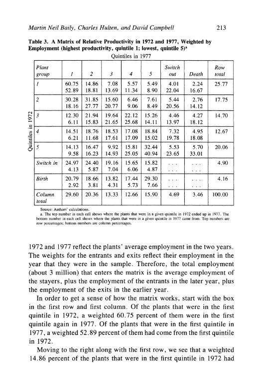
Martin Neil Baily, Charles Hulten, and David Campbell 213
Table 3. A Matrix of Relative Productivity in 1972 and 1977, Weighted by Employment (highest productivity, quintile 1; lowest, quintile 5)"
Quintiles in 1977
Plant Switch Row group 1 2 3 4 5 out Death total
1 60.75 14.86 7.08 5.57 5.49 4.01 2.24 25.77 52.89 18.81 13.69 11.34 8.90 22.04 16.67
2 30.28 31.85 15.60 6.46 7.61 5.44 2.76 17.75 18.16 27.77 20.77 9.06 8.49 20.56 14.12
3 12.30 21.94 19.64 22.12 15.26 4.46 4.27 14.70 _ 6.11 15.83 21.65 25.68 14.11 13.97 18.12
4 14.51 18.76 18.53 17.08 18.84 7.32 4.95 12.67 6.21 11.68 17.61 17.09 15.02 19.78 18.08
5 14.13 16.47 9.92 15.81 32.44 5.53 5.70 20.06 9.58 16.23 14.93 25.05 40.94 23.65 33.01
Switch in 24.97 24.40 19.16 15.65 15.82 . . . . . . 4.90 4.13 5.87 7.04 6.06 4.87 . . . ...
Birth 20.79 18.66 13.82 17.44 29.30 . . . . . . 4.16 2.92 3.81 4.31 5.73 7.66 . .. . ._._ .
Column 29.60 20.36 13.33 12.66 15.90 4.69 3.46 100.00 total
Source: Authors' calculations. a. The top number in each cell shows where the plants that were in a given quintile in 1972 ended up in 1977. The
bottom number in each cell shows where the plants that were in a given quintile in 1977 came from. Top numbers are row percentages; bottom numbers are column percentages.
1972 and 1977 reflect the plants' average employment in the two years. The weights for the entrants and exits reflect their employment in the year that they were in the sample. Therefore, the total employment (about 3 million) that enters the matrix is the average employment of the stayers, plus the employment of the entrants in the later year, plus the employment of the exits in the earlier year.
In order to get a sense of how the matrix works, start with the box in the first row and first column. Of the plants that were in the first quintile in 1972, a weighted 60.75 percent of them were in the first quintile again in 1977. Of the plants that were in the first quintile in 1977, a weighted 52.89 percent of them had come from the first quintile in 1972.
Moving to the right along with the first row, we see that a weighted 14.86 percent of the plants that were in the first quintile in 1972 had

214 Brookings Papers: Microeconomics 1992
moved down to the second quintile by 1977. This is a huge drop com- pared with the percentage that had stayed in the first quintile. These percentages gradually decrease along the row. Only a weighted 4.01 percent of the top 1972 plants had switched out of this industry by 1977 and only 2.24 percent had closed.
Of the plants that were in the top quintile in 1977, a weighted 52.89 percent of them came from the top quintile in 1972. As we move down the first column of the boxes, the percentages again decline, although not monotonically. Of the plants that were in the first quintile in 1977, 9.58 percent had been in the fifth quintile in 1972. Only about 7 percent of the plants that were in the top quintile in 1977 were plants that had switched in to this industry (4.13 percent) or were new entrants (2.92 percent).
The plants have been divided into quintiles on the basis of number of plants. When the plants are weighted by employment, however, the quintiles are far from even. Employment is more concentrated in the top and the bottom quintiles (See appendix table A-3 to compare the weighted and unweighted matrices.)
In the 1972-77 transition matrix, we are impressed by the persistence in the relative productivity. This persistence seems to be particularly marked at the top of the distribution. The somewhat lower persistence at the bottom is to be expected since these plants have the opportunity to change industry or to close down as well as to move up.
There is not much evidence in table 3 of a systematic plant vintage effect. Of the plants that were in the second quintile in 1972, more of them (on a weighted basis) moved into the top quintile than into the third quintile. Of the plants that were in the third quintile in 1972, about the same number had moved into the first and second quintiles as had moved into the third and fourth quintiles. In addition, the new plants were not all concentrated in the top quintiles.
The kind of cycling that is predicted by the innovative remnant model describes some but not most of the plants in table 3. For example, of the plants that were in the bottom quintile in 1972, a weighted 30.36 percent of them (14.13 + 16.23) were in the first two quintiles in 1977. Of the plants that were in the top quintile in 1977, 9.58 percent of them were plants that had come from the bottom quintile in 1972. The same pattern is present, although less marked, in the 1977-82 and 1982-87 matrices (not shown in this paper). The data show that some plants with

Martin Neil Baily, Charles Hulten, and David Campbell 215
poor productivity can restructure and move up dramatically, but this is not the main pattern.
When we examine the entrants as a group, we see that the plants that switched out of their industries were spread fairly evenly through the quintiles. The concentration was somewhat greater at the top and the bottom. Plants that are doing badly will leave, but many high- productivity plants may see better opportunities in another product line. Plants that died are concentrated at the bottom of the productivity dis- tribution. A weighted 51.09 percent of them (18.08 + 33.01) came from the bottom two quintiles. Many low-productivity plants do not make it. If we look at the unweighted figures, the concentration of exits in the bottom quintiles is much more marked. Many of the low-pro- ductivity plants that do not make it are small. This fits well with the dynamic models of Jovanovic and Ericson and Pakes.26
A surprising number of high-productivity plants also exit the indus- try. In fact, there is a sign of bimodality in the distribution of exiting plants, if we look at switch outs and deaths. This slight bimodality reappears for the entrants and for subsequent time periods. Clearly, the data do not fit exactly with a model in which the only reason for exit is that the plant has fallen below some critical productivity level.
Looking at the entrants for 1972-77, we see that in the weighted data, the plants that switch in to an industry are somewhat concentrated in above-average productivity quintiles. A weighted 49.37 percent are in the first two quintiles. The pattern is less marked among the births, but there is fairly clear evidence of bimodality. The unweighted data reveal that it is the large entrants that have high productivity. In terms of numbers of plants, entrants are concentrated in the bottom quintiles.
The transition matrices for the 23 industries for the second and third time periods (not shown) reveal some patterns that are repeated over time and some patterns that change. The most interesting change in the pattern of transitions is that there is less persistence at the top of the distribution. This makes sense. During the 1980s, there was a lot of structural change in U.S. manufacturing. U.S. companies were forced to face very strong foreign competition as a result of the strong dollar. And foreign manufacturers were opening new plants in the United States or were upgrading existing plants that they purchased.
26. Jovanovic (1982); and Ericson and Pakes (1989).

216 Brookings Papers: Microeconomics 1992
Table 4. A Matrix of Relative Productivity in 1972 and 1982, Weighted by Employment (highest productivity, quintile 1; lowest, quintile 5)"
Quintiles in 1982
Switch Switch Plant out out Dead Dead Row group 1 2 3 4 5 1977 1982 1977 1982 total
1 42.48 15.70 7.35 7.66 13.04 3.92 3.32 2.35 4.18 23.52 46.48 25.34 15.17 12.97 14.34 22.66 19.96 16.01 16.93
2 19.01 19.57 18.62 12.40 10.26 4.88 5.29 2.96 6.99 16.78 14.84 22.52 27.39 14.97 8.05 20.15 22.72 14.42 20.18
3 14.45 14.48 11.68 17.38 16.84 4.30 5.01 4.62 11.25 13.71 9.21 13.61 14.04 17.15 10.79 14.51 17.57 18.36 26.51
4 9.25 14.59 10.69 14.57 26.94 7.39 4.17 5.22 7.19 12.04 ______ 5.18 12.05 11.28 12.62 15.16 21.87 12.84 18.24 14.88
a 5 8.34 8.37 7.38 15.49 38.32 4.36 5.43 5.86 6.44 19.39 7.52 11.14 12.56 21.61 34.74 20.81 26.92 32.97 21.49
Cv Switch 20.41 19.07 13.70 17.77 29.05 ... ... ... ... 3.16 in 1977 3.00 4.14 3.80 4.05 4.30 ... ... ... ...
Switch 24.55 14.01 18.61 20.28 22.56 ... ... ... ... 4.79 in 1982 5.47 4.60 7.82 6.99 5.05 ... ... ... ...
Born 23.35 17.54 13.43 22.25 23.43. ... ... 3.31 1977 3.60 3.99 3.90 5.30 3.63 ... ... ... ...
Born 30.64 11.58 13.98 18.24 25.55 ... ... ... ... 3.30 1982 4.70 2.62 4.04 4.33 3.94 ... ... ... .
Column 21.50 14.58 11.40 13.90 21.39 4.07 3.91 3.45 5.81 100.00 total Source: Authors' calculations. a. The top number in each cell shows where the plants that were in a given quintile in 1972 ended up in 1977. The
bottom number in each cell shows where the plants that were in a given quintile in 1977 came from. Top numbers are row percentages; bottom numbers are column percentages.
Because of the marked pattern of persistence in the 5-year transition matrices, we decided to take a look at the 10-year matrix for the 1972- 82 period. Table 4 gives the results for the weighted data; the un- weighted matrix is in appendix table A-4. The persistence in the 10- year transitions was even more remarkable than that found in the 5- year table. For plants in the top quintile in 1972, more than 58 percent of them were still in the top two quintiles in 1982 (42.48 + 15.70). This is for the weighted data, but even in terms of number of plants, the equivalent number is almost 47 percent. Of the plants that were in the bottom quintile in 1972, nearly 54 percent of them were in the

Martin Neil Baily, Charles Hulten, and David Campbell 217
Table 5. A Matrix of the Relative Productivity of Births in Quintile 1987 (highest productivity, quintile 1; lowest, quintile 5)
Quintile 1987
Plant group 1 2 3 4 5
Born 10-15 36.03 18.13 17.48 14.02 14.34 years ago 4.80 3.41 4.29 3.92 2.51
Born 5-10 years 28.41 31.37 5.93 9.94 24.35 ago 3.64 5.66 1.40 2.67 4.10 Born less than 5 19.03 10.78 11.87 18.89 39.44 years ago 4.23 3.37 4.85 8.79 11.52
Source: Authors' calculations.
bottom two quintiles 10 years later (15.49 + 38.32). Just over 22 percent of these plants had died or left the industry (4.36 + 5.43 + 5.86 + 6.44). These are all size-weighted figures.
We also have constructed 15-year transition matrices for the entire 1972-87 period. There is a good deal of persistence evident in these matrices, although less than for the 10-year transitions. The reason that we did not use the full 15-year period is that there were changes made in the SIC and in the LRD for 1987. Some industries were redefined, and so we had to track down plants and try to keep our industry defi- nitions consistent. More problematic was the fact that some plants were divided into two, and some plants were combined into one. We have spent a good deal of time trying to overcome this problem by tracking down the changes, but there remain too many deaths in our 1987 sample for us to have confidence in the results.
Although also somewhat uncertain, results for births from the 1987 sample are sufficiently interesting to be reported (table 5). We give the part of the transition matrix that shows where the births ended up. In the 5-year matrices births enter with rather low productivity.27 In the 10-year transition, births gradually caught up to the average level of productivity.28 Following the plants over the 15-year horizon reveals an important new finding: the plants that were born between the 1972 and 1977 censuses have above average productivity by 1987. These results are conditional, of course, upon the plants having survived. We
27. Other researchers using similar data sets have found the same pattern. See Griliches and Regev (forthcoming); and Bregman, Fuss, and Regev (forthcoming).
28. For Canada, Baldwin and Gorecki (1990) found the same thing.

218 Brookings Papers: Microeconomics 1992
find that the survivors move up the distribution, or the ones at the bottom are weeded out over time, or both effects are in operation.
We have made some inferences that were based on inspection of the transition matrices, but we can do better than that by verifying the patterns statistically. Some simple nonparametric tests relate directly to the patterns of movement in the transition matrices.
Testing the Productivity Rankings
In the process of constructing the transition matrices, we ranked the plants on the basis of their relative productivities. The extent to which stayers, entrants, and exits have different productivity ranks can be used for hypothesis testing. Statistical analysis based upon ranks has a long history in economics. Two of Milton Friedman's earliest articles proposed nonparametric methods that are still used today.29 We will use the Wilcoxon statistic, a simple nonparametric test that asks whether the ranks of some "treatment" group of plants is different from the ranks of a control group.30 Under the null hypothesis of no difference between the treatment group and the control group, the rankings of the treatment group of plants will be scattered randomly, regardless of the true distribution of productivity. This allows the computation of a stan- dard normal test statistic that can reject the null for large samples.
In the tests for the 1972-77 panel, for example, we look at all of the plants in operation in 1977. For the plants that were also operating in 1972, we take the group that was in, say, the first quintile in 1972. Then we see how the plants rank in the productivity distribution in 1977. We do the same for the plants that were in the four other quintiles in 1972. We also look at the plants that switched in to the industry and the births between 1972 and 1977. We see how they are ranked in 1977.
The first column of table 6 gives standard normal test statistics based upon the rankings of the plants in 1977. Plants are divided into groups depending upon their quintile in 1972 or whether they are switch-ins or births.31 Plants that were in the first and second quintiles in 1972
29. Friedman (1937, 1940). 30. Diebold and Rudebusch (forthcoming) describe the approach. 31. The results reported in table 6 do not adjust for differences in the size of plants.
They correspond to the unweighted results.

Martin Neil Baily, Charles Hulten, and David Campbell 219
Table 6. Wilcoxon Tests of Productivity Transitions
Test of rank Test of rank Test of rank in 1977 in 1982 in 1987
based on based on based on 1972 1977 1982
Plant group quintile quintile quintile
First quintile - 20.35 -17.78 - 16.89 Second quintile -7.69 -5.18 -7.75 Third quintile 1.52 0.91 0.68 Fourth quintile 4.48 4.90 4.80 Fifth quintile 6.42 8.30 7.83 Switch ins 4.80 6.96 7.27 Births
Less than 5 years ago 13.20 7.71 7.10 5 to 10 years ago . . . 0.99 0.35 10 to 15 years ago ... ... -2.20
Source: Authors' calculations.
were significantly above average in relative productivity when ranked in 1977. The standard normal statistic is negative, which indicates a low rank. In other words, these are plants near the top of the productivity distribution. (The lowest numerical rank is equal to unity, the top plant.) Plants ranked in the bottom two quintiles in the early years have relative productivities that were significantly below average in the later period. Similar results apply to the 1977-82 and 1982-87 periods, but we have not included these in the table.
It is, perhaps, not surprising to find that plants in the top quintiles in a given year were still well above average in productivity four or five years later. But the results from the 10-year transitions (not shown) are really quite strong: plants in the top two quintiles in 1972 were still ranked way above average 10 years later. There is clearly an enormous amount of persistence in the productivity distribution.
The results for the entrants during the five-year period are interesting. Recent births have relative productivities well below the average. In fact, the new entrants rank well below the stayers that were in the bottom quintile in the early period, based upon the sizes of their standard normal statistics. We find, as others have found before us, that plants that enter an industry have low productivity on average. The plants that switch to this industry are also below average in productivity, according to the Wilcoxon tests.

220 Brookings Papers: Microeconomics 1992
Table 7. Wilcoxon Tests of the Productivity of Exits
Rank Rank Rank in Plant group in 1972 in 1977 1982
Switch outs 5 years hence 5.85 7.49 5.22 5 to 10 years hence 3.17 1.02 ... 10 to 15 years hence 1.25 ... ...
Deaths 5 years hence 8.46 12.16 8.95 5 to 10 years hence 5.11 6.19 10 to 15 years hence 3.17 . . ....
Source: Authors' calculations.
When we look at the tests over 10 years, we see a big difference
between the entrants that came in the 1972-77 period and those that
came in the 1977-82 period. The plants that entered in the earlier period
and had not exited again had just about caught up to the average by
1982. And this pattern shows up even more for the survivors over 15
years. These plants are significantly above average in productivity by
1987, as shown in the last column of table 6.
The transition matrices show not only where plants had come from
but also where plants had moved to. In particular, we can look at the
plants that were in operation in an early year and had left the industry
or closed down by the later year. Plants that exited the industry by
switching out or closing down were below average in rank 5 years, 10
years, or 15 years prior to their exit (table 7). This is the average pattern,
and it is one that we expected to see. Recall, however, that there are
high-productivity deaths in all of the industries, particularly when the
plant that closes is a large plant.
Transitions Based on Productivity Bands
The transition matrices that we have tabulated have a distinctive
feature: a spreading of productivity among the plants in the middle
quintiles. The extent of persistence looks lower for the middle quintiles. This occurs partly because the distribution of productivities is roughly
bell shaped and so the range of productivities is narrower for the middle
quintile than it is for the top or bottom quintiles. Plants are likely to

Martin Neil Baily, Charles Hulten, and David Campbell 221
move across quintiles more easily in the middle of the distribution.32 In a pioneering analysis of business concentration, P.E. Hart and S.J. Prais discuss this issue and present transition matrices based on quintiles and on equal width productivity bands.33 The quintiles ask, for example, whether plants in the top fifth of plants remain in the top fifth over time. The band transitions ask, for example, whether plants that are 25 to 50 percent above the industry average productivity will remain in the same band over time. There is no particular rule that says that quintiles or bands are better; they simply look at different questions.
To illustrate more fully what is happening in the middle of the pro- ductivity distribution, we present histograms (figure 2) showing how plants that were in a given productivity band in 1982 were distributed in 1987. We are showing a partial representation of the joint productivity distribution. The open-ended top and bottom bands with very few plants are omitted. We present the results for the 1982-87 period since this period was neglected in our earlier analysis. Because we are concerned about the reliability of the data, deaths are omitted. The results for band transitions for the earlier time periods look very similar to the results depicted in figure 2.
Persistence will show up in figure 2 if the mass of the distribution is concentrated around the same band in 1987 that the plants had in 1982. In general, the figure provides support for persistence in the distribution within the center of the bell-shaped distribution.
This concludes our examination of the transition matrices and the nonparametric tests that are based upon them. There is very striking persistence to the productivity distribution and wide diversity among different plants, including differences among entrants and exiters. We now explore how the observable characteristics of plants affect the levels and rates of growth of productivity of the plants in our sample.
Regression Analysis of Productivity
We ask whether relative productivity can be explained by plant char- acteristics. We use the term "explain" cautiously, however. At this
32. We are grateful to Richard Caves and Peter Reiss for helpful comments on this issue.
33. Hart and Prais (1956).

222 Brookings Papers: Microeconomics 1992
Figure 2. Distribution of Productivity in 1987, Conditional on TFP in 1982
TFP in 1982 = -0.75 to -0.5 TFP in 1982 = -0.5 to -0.25
Percent Percent 50 50 -
40 40 -
30 - 30-
20 -20-
10 I 10 -
<-1-.75 -.5 -.25 0 .25 .5 .75 >1 <-1-.75-.5-.25 0 .25 .5 .75 >1
TFP in 1982 =-0.25 to 0 TFP in 1982 =O to 0.25
Percent Percent 50 - 50
40 - 40
30 -30-
20 20
10 10
0 0 <-1-.75 -.5 -.25 0 .25 .5 .75 >1 <-1-.75-.5-.25 0 .25 .5 .75 >1
TFP in 1982 = 0.25 to 0.5 TFP in 1982 = 0.5 to 0.75
Percent Percent 50 -50-
40 40
30 30-
20 20 -
10 10
0 0 <-1-.75-.5-.25 0 .25 .5 .75 >1 <-1-.75-.5-.25 0 .25 .5 .75 >1
Source: Authors' calculations.

Martin Neil Baily, Charles Hulten, and David Campbell 223
point we are mostly looking for correlations that will allow us to char- acterize high- and low-productivity plants. As well as asking why one plant is more productive than another in a given year, we explore the relative rates of productivity growth among plants and whether there are correlates with high and low growth. We separate the stayers, the entrants, and the exits.
Wage rates for production workers and plant productivity are strongly correlated. High-productivity plants pay high wages. We explore what drives this correlation.
The production function provides a standard framework for explain- ing the distribution of productivities across plants with the usual factor inputs. It also can test the importance of other plant characteristics. We estimated many production functions for the time-series cross-sectional data on the five industries we studied initially. All of the factors of production were statistically significant and had coefficients in a Cobb- Douglas function that were reasonably close to the factor income shares. (The capital share was often too low.) R-squareds were very high. In other respects, however, the results were not so good. Estimates of translog or restricted translog functions showed that second-order terms were highly significant, but the resulting coefficients failed concavity tests.
Given possible concerns about functional form, not to mention issues of endogeneity and selection bias, we decided to use relative TFP (or the rate of plant TFP growth), rather than output, as the dependent variable in our regressions. Since this procedure assigns cost shares as the factor elasticities and allows for different implied elasticities across plants and industries, it gives us an important advantage. It allows us to pool the 23 industries (with industry intercept dummies included) in order to test hypotheses common to all industries, such as the importance of past productivity or the importance of firm effects.
When the relative TFP computation is made from cost shares, the sum of the factor elasticities may add up to more or less than unity. We are not imposing constant returns to scale. Therefore, in our regres- sions we include size dummies based on employment to pick up any residual scale effect. Scale effects could occur if large and small plants differ in the extent to which they have market power in product or factor markets, or they could occur because high-productivity plants have been able to become large. The size dummies do not provide a good test of

224 Brookings Papers: Microeconomics 1992
increasing or decreasing returns to scale within the production function itself. Therefore, we ran cross-sectional production functions for each of the 23 industries for each census year. We report tests of returns to scale from these estimates.
Results for Stayers
The main results for the plants that were operating at both the be- ginning and the end of the period are shown in table 8. All of the regressions contain dummy variables to adjust the intercept for industry and regional differences. Although we have not shown the coefficients on these dummy variables, F tests indicate that they are statistically significant. The other main findings are as follows.
First, an important determinant of productivity in the given year is the productivity of the plant five years earlier. Plant-level fixed effects in productivity are persistent.
Second, plants that are part of a high-productivity firm also will have high productivity. (Firm productivity for plant i is defined as the average productivity of plants in the same firm other than plant i.) Well-run firms will be able to transfer those skills to their plants by training managers, giving advice, and transferring technology, good product design, and production methods.
Third, in the OLS regressions the plant relative wage enters with a very significant coefficient and a magnitude roughly equal to the share of wages in total cost.
Fourth, large plants (the omitted size category) may have higher relative TFP than do small plants. This size effect diminishes over time.
Fifth, plants that specialize in a single product may or may not be more productive. Our data did not provide much evidence on this question.
Sixth, there is rather weak evidence for plant vintage effects. In table 8 we include dummies to give a rough indication of plant age. The first dummy is unity if the plant was in operation in the 1963 census-a "pre-1963" plant. We did the same thing for plants that were first observed in later censuses. The results are not terribly strong, but they are consistent with the hypothesis that there is a small plant-vintage effect. Old plants are less productive.
Keep in mind that the contribution of all capital to output is small,

Martin Neil Baily, Charles Hulten, and David Campbell 225
Table 8. Regressions for Stayersa
Estimated OLS 2SLS parameters (t-statistics) 1977 1982 1987 1977 1982 1987
TFP 5 years ago 0.30 0.35 0.31 0.29 0.34 0.30 (19.3) (16.9) (15.0) (16.4) (13.4) (11.1)
Firm TFP 0.28 0.19 0.19 0.27 0.20 0.25 (12.7) (7.7) (6.4) (10.2) (6.2) (6.6)
Wage 0.18 0.16 0.19 0.04 -0.12 0.08 (9.3) (7.0) (7.3) (0.6) (-1.3) (0.6)
Size Less than 25% -0.12 0.00 -0.07 -0.13 -0.02 -0.06
(-8.1) (0.0) (-2.8) (-7.1) (-0.9) (- 1.9) 25% to 50% -0.06 0.02 -0.05 -0.07 -0.00 -0.05
(-5.3) (1.2) (-2.5) (-4.6) (-0.1) (-2.0) 50% to 75% -0.03 0.01 -0.02 -0.04 -0.02 -0.03
(-3.1) (0.4) (- 1.4) (-2.9) (- 1.1) (- 1.3) Specialization -0.02 0.05 0.05 -0.02 0.06 0.03
ratio (5-digit) (-0.8) (1.6) (1.2) (-0.8) (1.7) (0.6) Age
Pre-1963 -0.04 -0.01 -0.04 -0.02 0.04 -0.01 (-2.6) (-0.6) (- 1.3) (- 1.2) (1.4) (-0.4)
Pre- 1967 -0.03 -0.01 0.03 -0.03 0.02 0.04 (-1.8) (-0.2) (0.8) (-1.4) (0.8) (1.1)
Pre-1972 0.01 0.02 0.03 0.04 (0.6) (0.6) (1.0) (0.9)
Pre- 1977 . . . . .. 0.02 . . . . .. 0.03 (0.6) (0.7)
Single unit 0.01 0.03 0.01 -0.01 -0.03 0.00 (0.4) (1.0) (0.3) (-0.4) (-0.8) (0.1)
Single plant of 0.03 0.02 -0.01 0.02 0.01 -0.02 multi-unit firm (2.7) (1.7) (-0.7) (1.4) (0.4) (-0.8)
R2 0.32 0.23 0.22 0.27 0.19 0.17 Number of
observations 3,124 2,770 2,363 2,539 2,178 1,814 Source: Authors' calculations. a. The dependent variable is relative productivity. All regressions allow for industry fixed effects and regional effects.

226 Brookings Papers: Microeconomics 1992
and the contribution of the fraction of the capital in structures will be even smaller. We should not expect a big vintage coefficient. Old plants invest in new equipment capital and acquire new technology that way. In fact, large old plants differentially acquire new technology sooner than do small new plants.34
Seventh, spillover effects of being part of a multiplant firm are not a significant element in plant productivity. To try and capture spillover effects, we include two alternative variables: "single unit" (plants with no other plants in the same firm) and "single unit of multi-unit firm" (plants with other plants in the same firm but none in the same industry). Being part of a high-productivity firm is associated with a spillover benefit. But regardless of the specific productivity of the rest of the firm, there could be advantages to being part of a multiplant firm simply because the head office provides administrative or other services directly to its plants. In a single plant firm the administration is all performed at the single plant. We do not find this to be an important factor in practice.
Several of the variables that have been tested in table 8 will change little over time. They are part of the fixed characteristics of the plant. Including prior TFP in the regression may make it hard to estimate the effect of the variables such as the size dummies or the age dummies. Specialization may be important, but it is being picked up in prior TFP. Therefore, we have run the results in table 8 with the "TFP five years ago" variable omitted. We find that size becomes more important, high specialization ratios seem to reduce TFP, the vintage effects become a little stronger, and there is a significant disadvantage to being a single- unit firm. In other words, there is more support for the view that head offices provide services of value.
We have examined the residuals of our regressions for hetero- skedasticity and found little evidence of its importance. If anything, there is a slight tendency for greater variance among small plants, as one would expect if data errors are greater in the small plants.35 We ran some earlier results with the standard error correction suggested by
34. Dunne (1991). 35. Many people suggested to us that large plants would have greater error variance,
but the intuition on this is not correct. The dependent variable is relative productivity measured in logarithms. The error variance does not simply increase with size.

Martin Neil Baily, Charles Hulten, and David Campbell 227
White,36 but with many degrees of freedom and small heteroskedasticity to begin with, the correction had little effect. It reduced the standard errors only slightly. Since it took us many hours of computer time for such a small effect, we have not made the correction in the results given here.
Results for Entrants
The results for entrants are shown in table 9.37 We give results for productivity in 1977 of plants that entered between 1972 and 1977 and for productivity in 1982 of plants that entered between 1977 and 1982. The results for this latter group are fairly weak. The period from 1977 to 1982 was a difficult one for the manufacturing sector, so the 1982 column may not be typical for entrants. The 1977 results may be a better guide.
Our findings are as follows. Firm TFP is significant for entrants in 1977 but not in 1982. The relative wage results look more robust than they did for the stayers. There is no apparent productivity difference between plants that were births and plants that switched in from another industry. Entrants that specialize have somewhat higher productivity than do entrants that do not specialize. For plants that switched in from another industry, there are some advantages to being "middle-aged." Finally, being a single-unit entrant is a disadvantage. But for plants that are not single units, whether the other plants in the firm are in the same industry does not seem to be very important.
The Probability of Death
Equations examining the probability of death in the LRD plants have been estimated by Tim Dunne and Mark Roberts and by Steve Olley and Ariel Pakes, and we have made use of their findings.38 We present our own probability of exit regressions in table 10. The regressions show how the characteristics of plants in the given year affect the probability of plant death over the subsequent five-year period.
36. White (1980). 37. We do not include an entrants regression for 1987 because we have not been able
to identify the entrants with sufficient confidence. 38. Dunne and Roberts (1990); and Olley and Pakes (1992).

228 Brookings Papers: Microeconomics 1992
Table 9. Regressions for Entrantsa
Estimated coefficients OLS 2SLS (t-statistics) 1977 1982 1977 1982
Firm TFP 0.22 0.05 0.14 0.03 (5.0) (0.9) (2.9) (0.4)
Wage 0.28 0.30 0.33 0.30 (10.9) (9.9) (2.3) (1.1)
Switch ins 0.01 -0.05 0.03 -0.08 (0.3) (-1.5) (1.1) (-1.6)
Size Less than 25% -0.14 -0.04 -0.15 -0.02
(-4.5) (- 1.0) (-3.8) (-0.3) 25% to 50% -0.10 -0.03 -0.10 0.03
(-3.3) (-0.9) (-2.5) (0.4) 50% to 75% -0.08 0.04 -0.09 0.10
(-2.4) (0.9) (-2.4) (1.7) Specialization 0.09 0.13 0.06 0.08
ratio (5-digit) (2.1) (2.3) (1.4) (0.9) Age
Pre-1963 0.04 0.00 0.00 0.00 (1.2) (0.0) (0.0) (0.1)
Pre- 1967 0.06 0.09 0.04 0.08 (1.8) (1.8) (1.0) (1.0)
Pre-1972 . . . 0.07 . . . 0.12 (1.5) (2.0)
Pre- 1977 ... ... ... .
Single unit -0.08 -0.01 -0.06 -0.01 (-3.0) (-0.4) (- 1.8) (-0.1)
Single plant of multi-unit firm 0.04 0.02 0.02 0.01 (1.8) (0.7) (0.9) (0.3)
R2 0.25 0.25 0.23 0.20 Number of observations 1,145 798 719 453
Source: Authors' calculations. a. The dependent variable is relative productivity. All regressions allow for industry fixed effects and regional effects.
Employment size is by far the largest and most significant deter- minant of the probability of death. Large plants are much less likely to close down than are small plants. In addition, low productivity in a plant is strongly associated with the probability of death.
The probability of death of a given plant is influenced by the pro- ductivity of the TFP in other plants in the same firm. The coefficient, however, changes sign with the time period. Consider the 1972 regres-

Martin Neil Baily, Charles Hulten, and David Campbell 229
Table 10. Probability of Death Regressionsa
Estimated parameters Probit Probit (chi-square) 1972 1977
TFP -0.36 -0.41 (12.3) (17.5)
Firm TFP 0.33 -0.24 (5.1) (3.3)
Wage 0.31 0.30 (7.7) (10.3)
Size Less than 25% 1.21 0.97
(141.0) (123.4) 25% to 50% 0.78 0.51
(60.5) (35.8) 50% to 75% 0.50 0.43
(24.1) (25.7) Specialization -0.02 -0.01
ratio (5-digit) (0.02) (0.0) Age
Pre- 1963 -0.36 -0.35 (25.4) (22.2)
Pre-1967 -0.20 -0.17 (6.3) (3.8)
Pre- 1972 . . . -0.29 (11.7)
Pre-1977
Single unit -0.24 -0.23 (7.4) (6.7)
Single plant of multi-unit firm 0.05 -0.01 (0.5) (0.0)
Pseudo R2 0.15 0.11 Number of observations 4,517 4,631
Source: Authors' calculations. a. All regressions allow for industry fixed effects and regional effects.
sion. If the productivity of the given plant is held constant and if the other plants in the same firm have high productivity, then this plant is more likely to close. This finding is consistent with the idea that a firm will close its weak plants. The pattern is not sustained for exits over the 1977-82 period. Exit decisions were somewhat differently moti- vated during this difficult cyclical period. Notice, however, the large number of exits in both periods and the fact that the number of exits

230 Brookings Papers: Microeconomics 1992
is not all that much higher over the 1977-82 period than over the 1972- 77 period.
High-wage plants have an increased probability of closure (condi- tional upon the productivity of the plant). Old plants are much less likely to close than are new plants. Surprisingly, single-unit plants are less likely to close, after controlling for other variables, than are multi- unit plants. Finally, high product specialization has no impact on productivity.
Wages, Labor Quality, and Productivity
The regressions for the stayers and for the entrants have been esti- mated using two-stage least squares, with the wage treated as an en- dogenous variable. The plant wage is assumed to be determined by plant size and plant productivity and by a number of local labor market variables. These variables capture educational and demographic char- acteristics of the county in which the plant is located and the local unemployment rate. Plant productivity is taken to be endogenous. The productivity equation includes the variables we have described for the OLS results, except that the wage is taken as endogenous. The results of these two-stage regressions, shown in tables 8 and 9, were rather striking.
Among the plants that were stayers, productivity was a significant and important determinant of the wage, but the wage was no longer an important or significant determinant of productivity. Among the en- trants, productivity was an important and significant determinant of the wage, and the wage was an important and significant determinant of productivity. There was some weakening of statistical significance of the wage coefficient in the 1977-82 regression, although the size of the coefficient remained the same.
We substituted a fitted value of the wage for the actual value in the probit regression for plant closings. It appears that high wages are still an important reason for closings.
The results for stayers suggest that most of the correlation between wage and productivity in these established plants is the result of workers or unions being able to demand higher wages in plants that have high productivity. This is consistent with the rent-seeking model described

Martin Neil Baily, Charles Hulten, and David Campbell 231
by Katz and Summers.39 The exit probabilities also suggest that high wages are the result of wage demands. If high wages were the result only of the high quality of labor, then these wages should not increase the probability of closing.
For entrants there is more evidence that high wages are indicative of high-quality workers. Workers in entering plants have had less op- portunity to organize, so employers have been able to select on the basis of quality.
During the 1980s, direct foreign investment in the U.S. manufac- turing sector increased as more foreign plants began setting up opera- tions in this country. These transplants pay wages that are comparable to those of established U.S. plants, but the firms carry out a careful screening of production workers. The results here suggest that the ability of new entrants to select high-quality workers may be a significant advantage, offsetting possible disadvantages of being an entrant.
The results on wages and productivity are striking, but we urge caution in their interpretation. We are quite willing to believe that some part of the strong correlation between wages and productivity results from the ability of workers to extract rent. But it also seems plausible that plants that were forced to pay high wages could select high-quality workers to compensate for the high wages. An obvious problem with the results is that we do not have any direct measures of worker quality. 40
Results for the Rate of Productivity Growth
We ran regressions in which the dependent variable was the rate of productivity growth in a plant over the 1977-82 and 1982-87 periods. The main independent variables are the rate of plant productivity growth over the prior five-year period and the rate of growth of productivity in the other plants of the same firm. Consistency with the earlier regres- sions suggests that we should leave out variables, such as the size
39. Katz and Summers (1989). 40. Lester Telser and other members of the micro workshop at the University of Chicago
commented on our findings. They think the findings indicate simply that there was no correlation between productivity and the part of the wage that is associated with local labor market conditions. There is certainly something to this point. Note, however, that the plant characteristics that affect plant productivity (including size) are included in the instruments that determine the predicted plant wage.

232 Brookings Papers: Microeconomics 1992
dummies, that are pretty much plant fixed effects. But we decided to leave these variables in. There is no certainty that the earlier level equations are accurate structural relations. It is worth seeing whether there is any relation between size and age and productivity growth.
Both periods involve the recession year 1982. In the first five-year period the manufacturing sector is falling into recession, and in the second period it is growing out of recession. The first period in particular is unlikely to provide a good guide to the underlying correlates with longer term growth.
The results are shown in table 11. Only plants that have survived for at least 10 years can be included. The main findings are as follows.
First, there is a strong negative correlation between a plant's growth rate over a five-year period and its productivity growth over the prior five years. This is indicative of regression toward the mean, and it is consistent with there being significant measurement error in productiv- ity, or of there being random shocks. We can rule out the case where growth in one period is uncorrelated with growth in the prior period (figure iB).
Second, firm productivity growth strongly influences plant produc- tivity growth. There may be common productivity shocks that hit the plants in the same firm because of similarities in technology or product mix. And these "shocks" may not be simply random events. They could easily be the result of research and development or product de- velopment at the firm level.
Third, plants with high levels of investment (defined as purchases of equipment and structures) at the beginning of the growth period had slightly higher growth over the period. This applies only to the period of recovery from recession.
Fourth, size does not have a major impact on the growth rate. There is a slight sign that large plants do a little worse going into the recession, and this is then recovered in the subsequent growth period.
Fifth, high-wage plants grew a little more slowly than did low-wage plants in the recovery period. The wage is measured at the beginning of the five-year growth period.
Sixth, specialization has little impact on growth. Seventh, evidence of a vintage effect is stronger in these results than
in the earlier ones. During the recovery period, the oldest plants grew significantly more slowly than did the youngest plants. We now have

Martin Neil Baily, Charles Hulten, and David Campbell 233
Table 11. Regressions of Five-Year TFP Growth on Plant Characteristics, 1977-82 and 1982-87a
Estimated OLS 2SLS parameters 1977-82 1982-87 1977-82 1982-87
Wage -0.002 -0.04 0.03 -0.09 (- 0.1) (- 1.7) (0.3) (- 1. 1)
Prior TFP growth -0.31 -0.53 -0.31 -0.54 (5 years ago) (-14.8) (-21.5) (-13.4) (-19.3)
Firm TFP growth 0.13 0.25 0.11 0.27 (3.5) (6.5) (2.7) (6.3)
Investment -0.001 0.01 -0.001 0.01 (-0.2) (2.9) (-0.2) (2.2)
Size Less than 25% 0.02 -0.03 0.03 -0.03
(0.8) (- 1.2) (1.0) (- 1.1) 25% to 50% 0.01 -0.01 0.00 -0.02
(0.3) (-0.3) (0.0) (-0.7) 50% to 75% 0.02 0.01 0.01 -0.00
(1.5) (0.4) (0.7) (-0.2) Specialization -0.006 0.00 0.02 -0.01
ratio (5-digit) (-0.2) (0.0) (0.7) (-0.3) Age
Pre- 1963 0.01 -0.08 0.02 -0.08 (0.6) (- 3.4) (0.9) (- 2.8)
Pre- 1967 -0.00 -0.03 0.01 -0.03 (-0.1) (- 1.2) (0.6) (-0.9)
Pre- 1972 . . . -0.02 . .. -0.02 (-0.8) (-0.7)
Single unit -0.01 -0.01 0.01 0.00 (-0.1) (-0.2) (0.23) (0.1)
Single plant of multi-unit firm 0.02 -0.03 -0.03 -0.03 (1.2) (- 1.9) (- 1.9) (- 1.5)
R 2 0.11 0.38 0.23 0.39 Number of observations 2,132 1,902 1,830 1,589
Source: Authors' calculations. a. All regressions allow for industry fixed effects and regional effects.

234 Brookings Papers: Microeconomics 1992
Table 12. Estimated Returns to Scalea
Industry Number 1972 1977 1982 1987
Cotton mills 2211 1.048 0.975 0.951 0.946 Synthetic mills 2221 0.967 0.973 0.928 0.883* Softwood veneer 2436 0.992 0.995 0.964 0.939 Paper mills 2621 0.992 1.000 0.975 0.979 Paper board 2631 1.026 1.041 0.972 0.976 Inorganic chemicals 2819 0.967* 0.957* 0.977* 0.914*
Men's footwear 3143 1.034 1.016 0.938 0.939 Glass containers 3221 1.071 0.962 0.929 0.994 Pressed or blown glass 3229 1.026 0.999 0.976 0.928 Blast furnaces, steel 3312 0.979 0.969 0.964* 0.932* Nonferrous wire 3357 0.981 0.991 0.973 0.989 Metal containers 3411 0.933* 0.894* 1.032 0.960
Internal combustion engines 3519 1.007 0.984 1.026 1.033 Construction equipment 3531 0.982 0.954 0.960 0.979 Ball bearings 3562 0.943 0.945 0.980 0.977* Computer equipment 3573 0.976 0.958 0.939 0.957* Air conditioning machinery 3585 1.011 0.955* 0.981* 0.975 Electric motors 3621 1.001* 0.982 0.970 0.936
Glass housewares 3634 1.031 1.015* 0.994* 0.976* Telephone and telegraph equipment 3661 1.005 1.003* 0.980 0.956 Batteries 3691 0.951 1.025 0.971 0.904* Auto assembly 3711 1.008 1.045* 0.999 0.980 Auto parts 3714 0.999 0.978* 0.987 0.964*
Source: Authors' calculations. a. Asterisks indicate that the estimate is significantly different from I at the 5 percent level.
some sign of life-cycle aging, although the full story of plant life cycles is obviously complex. We had not uncovered much evidence of vintage effects in our earlier results, and we see here that old plants do as well as young plants going into a recession. We also have found that old plants have a much higher probability of survival than young plants. More work on plant life cycles is needed.
Finally, single-plant firms were at a growth disadvantage.
Returns to Scale
Table 12 shows the results of our empirical exploration of returns to scale in each industry for 1972, 1977, 1982, and 1987. The general word among researchers at the Center for Economic Studies at the Census Bureau has been that there are constant returns to scale in the

Martin Neil Baily, Charles Hulten, and David Campbell 235
LRD panel. Our results are unlikely to change that conclusion. If any- thing, there is some sign of decreasing returns, especially in the later years, but a vote for constant returns at the plant level looks like a pretty good bet.
There is nothing in this finding to refute current growth models that assume increasing returns. These models assume that there are increas- ing returns that derive from externalities of some kind.
Size had a positive impact on relative productivity in the regressions with relative productivity as the dependent variable. We found constant returns in the production function, however. This suggests that there is not perfect competition in product markets. Large plants are more likely than small plants to have a unique product or process technology.
Conclusions
We can now look back to the four alternative patterns that we dis- cussed at the beginning of the paper and presented in figure 1. Which one (or more) has the data supported? The answer is fairly clear. The overall pattern of the data is best described as a combination of the random shock/measurement error case (figure IA) and the plant fixed effects case (figure ID). The regression toward the mean and many other signs show the importance of the random shocks. The strong persistence, visible most dramatically in the 10-year transition matrix, supports the plant fixed effects framework.
It is no surprise to find that measurement errors and random shocks are an important part of the distribution of productivity in the LRD. We have spent enough time studying the individual observations to realize that true productivity in these plants is not known. And there will be important plant-specific shocks that will cause even an accurately measured productivity measure to move around. The more interesting finding is that there is strong persistence in relative productivity. The results on wages and productivity suggest that differences in worker quality may not be the main reason for the persistence of relative pro- ductivity. What appears to be important is management quality, broadly interpreted to include technology choice and product choice. Of course, this conclusion is tentative since we lack direct evidence on management quality.

236 Brookings Papers: Microeconomics 1992
Among the alternative variations on the theme of management qual- ity, we did not find the negative skewness that was implied by the Caves and Barton model. Nor did we see clear evidence for the "span of control" effects postulated by Lucas, although we did not disprove these. Somewhat by default, therefore, we find support for the kind of framework suggested by Kim Clark. In his case studies he finds that well-run plants perform at an above average level over long periods, and poorly run plants can remain weak for long periods. Like coaches whose teams continue to do well despite changes in personnel, there are good management teams whose plants continue to do well even with changing market conditions or technology.
When we compare the early time period in the mid-i1970s with the later periods, we find signs of change in the productivity distribution and in the pattern of entry and exit. We do not have a clear statistical test of difference, but it looks as though there was more entry and more mobility occurring in the later period of rapid productivity growth.
The innovative remnant model did not characterize the majority of plants, although there were examples of plants at the bottom of the distribution that were able to move up to the top.
Old plants are only slightly less productive than are more recent plants. The strongest effect of plant vintage is shown in the productivity growth results for the post-1982 recovery period.
In terms of numbers of entrants and exits and the forces that determine exit, there is evidence to support the models of plant dynamics devel- oped by Jovanovic and by Ericson and Pakes. But the majority of the entrants and exits are very small plants. They are something of a side- show to the overall performance of manufacturing industries.
A typical entering plant and a typical exiting plant have productivity well below average. This is by no means a universal pattern, however. There are high-productivity entrants and exits, particularly among the large entrants and exits.
The average productivity of new plants does rise relative to the average for all plants. This is because the smaller and lower productivity plants exit, leaving the higher productivity entrants as the survivors. In addition, the entrants grow more rapidly than average.
The growth of output shares in high-productivity plants is a major factor in the average productivity growth of the industries in our sample taken as a whole. Plants successful in productivity are gaining output

Martin Neil Baily, Charles Hulten, and David Campbell 237
share, and plants low in relative productivity are losing share, and this shifts the industry toward a higher productivity average.
One of the main correlates with productivity is relative wage. Plants with high productivity pay their workers more than do plants with low productivity. New entrants that pay high wages, it seems, can obtain high-quality workers, but old plants cannot take advantage of their high wages. This is reinforced by the finding that paying a high wage does seem to contribute to the probability of plant closure.
In conclusion we note the strong level and rate of growth effects from other plants in the same firm. There are common characteristics associated with plants in the same firm, including firm-level activities that generate growth for all plants.
APPENDIX
Table A-1. Decomposition of TFP Growth by Industry, Selected Periods Percentage increase over the period
Entry Fixed Share and
Industry Number Total shares effect exit
1972-77 Cotton mills 2211 - 13.14 - 16.80 3.02 0.64 Synthetic mills 2221 6.40 2.56 2.77 1.07 Softwood veneer 2436 -14.77 -18.30 1.29 2.24 Paper mills 2621 14.85 13.82 0.70 0.33 Paper board 2631 6.90 6.63 0.74 -0.47 Inorganic chemicals 2819 5.77 1.28 2.39 2.10
Men's footwear 3143 -7.81 -11.40 3.98 -0.40 Glass containers 3221 0.71 0.33 0.19 0.18 Pressed or blown glass 3229 -4.17 -7.02 3.74 -0.88 Blast furnaces, steel 3312 -1.91 -1.86 0.94 -0.99 Nonferrous wire 3357 13.37 11.47 0.88 1.01 Metal containers 3411 2.50 -0.76 2.10 1.16
Internal combustion 3519 0.77 3.61 0.51 - 3.34 engines
Construction equipment 3531 -11.51 - 15.73 4.38 -0.16 Ball bearings 3562 - 1.89 - 2.31 0.65 -0.23 Computer equipment 3573 87.88 76.16 8.58 3.15 Air conditioning 3585 4.77 4.29 1.25 0.78
machinery Electric motors 3621 1.18 2.05 2.19 -3.07

238 Brookings Papers: Microeconomics 1992
Table A-1 (continued)
Entry Fixed Share and
Industry Number Total shares effect exit
Glass housewares 3634 30.13 23.96 6.18 -0.02 Telephone and 3661 -4.39 -7.03 2.78 -0.15
telegraph equipment Batteries 3691 12.64 10.16 2.58 -0.10 Auto assembly 3711 13.46 11.44 2.11 -0.09 Auto parts 3714 -0.81 -4.17 2.49 0.87
1977-82 Cotton mills 2211 5.23 1.41 2.19 1.62 Synthetic mills 2221 - 1.53 - 3.69 1.85 0.31 Softwood veneer 2436 5.46 1.24 1.13 3.08 Paper mills 2621 5.68 3.07 2.34 0.27 Paper board 2631 2.74 0.84 1.66 0.24 Inorganic chemicals 2819 - 13.24 - 19.96 3.92 2.80
Men's footwear 3143 -0.33 -6.05 4.59 1.13 Glass containers 3221 - 8.62 - 10.26 0.80 0.83 Pressed or blown glass 3229 -12.03 - 11.01 2.95 -3.98 Blast furnaces, steel 3312 -3.66 - 7.86 4.62 -0.41 Nonferrous wire 3357 5.31 2.51 2.70 0.09 Metal containers 3411 - 3.27 -5.60 3.39 - 1.06
Internal combustion 3519 -14.74 -21.38 3.60 3.03 engines
Construction equipment 3531 - 8.29 - 11.63 4.14 -0.80 Ball bearings 3562 - 13.10 - 16.42 4.70 - 1.38 Computer equipment 3573 87.58 75.31 3.17 9.10 Air conditioning 3585 2.17 0.78 1.92 -0.52
machinery Electric motors 3621 - 10.83 -14.29 3.13 0.33
Glass housewares 3634 -9.94 - 13.99 2.46 1.59 Telephone and 3661 14.58 11.39 2.85 0.35
telegraph equipment Batteries 3691 - 3.29 - 3.61 0.82 -0.50 Auto assembly 3711 0.94 0.83 0.14 -0.02 Auto parts 3714 -18.20 -25.17 4.51 2.46
1982-87 Cotton mills 2211 12.92 15.82 1.72 -4.62 Synthetic mills 2221 12.63 9.12 0.78 2.73 Softwood veneer 2436 11.70 15.42 0.64 -4.36 Paper mills 2621 2.91 1.50 1.38 0.03 Paper board 2631 13.33 12.42 0.88 0.04 Inorganic chemicals 2819 10.57 7.75 2.07 0.75
Men's footwear 3143 12.37 5.76 2.89 3.71

Martin Neil Baily, Charles Hulten, and David Campbell 239
Table A-1 (continued)
Entry Fixed Share and
Industry Number Total shares effect exit
Glass containers 3221 9.21 6.94 1.69 0.58 Pressed or blown glass 3229 7.78 0.59 8.00 -0.81 Blast furnaces, steel 3312 18.30 19.38 1.44 -2.51 Nonferrous wire 3357 13.07 12.58 1.57 - 1.08 Metal containers 3411 - 3.69 - 8.16 1.88 2.58
Internal combustion 3519 10.72 7.72 3.38 - 0.38 engines
Construction equipment 3531 4.13 -2.27 6.58 -0.18 Ball bearings 3562 6.39 4.38 0.49 1.52 Computer equipment 3573 78.81 73.97 6.35 - 1.50 Air conditioning 3585 1.55 -3.89 3.97 1.47
machinery Electric motors 3621 -3.14 - 10.20 7.70 -0.64
Glass housewares 3634 4.18 - 1.21 3.60 1.79 Telephone and 3661 13.19 11.29 5.75 -3.85
telegraph equipment Batteries 3691 16.30 14.72 0.97 0.60 Auto assembly 3711 8.23 6.16 3.33 -1.27 Auto parts 3714 8.72 8.40 2.52 -2.20
Source: Authors' calculations.

Table
A-2.
Decomposition of
Stayers'
TFP
Growth
by
Position in
Productivity
Distribution,
Selected
Periods
Percentage
increase
over
the
period
Plants
that
Plants
that
Plants
that
Plants
that
Total
moved up
stayed in
moved
down
stayed in
(without
by
two or
more
top
two
by
vto or
more
bottom
two
The
rest of
Industrya
entry
and
exit)
quintiles
quintiles
quintiles
quintiles
the
plants
1972-77
2211
Growthb
-0.17
-14.07
-46.41
-10.94
-17.94
Contributionc
-13.78
1.22
0.90
-9.48
-1.12
-5.30
2221
Growth
53.05
-2.51
-28.18
10.32
9.59
Contribution
5.33
10.93
-1.16
-9.43
0.22
4.77
2436
Growth
10.31
15.47
-37.48
-13.69
-13.76
Contribution
-17.01
5.16
-1.50
-16.61
-2.46
-1.60
2621
Growth
33.96
12.07
-5.89
13.45
12.00
Contribution
14.52
7.08
1.41
-2.18
4.31
3.91
2631
Growth
35.65
11.05
-17.02
9.34
8.83
Contribution
7.37
4.68
2.99
-8.21
3.89
4.02
2819
Growth
45.60
-3.51
-54.06
3.88
12.06
Contribution
3.67
7.60
-0.86
-4.10
-1.39
2.43
3143
Growth
22.24
-8.66
-49.06
-5.37
-5.86
Contribution
-7.42
7.80
3.01
-16.65
-0.90
-0.68

3221
Growth
20.43
-1.37
-13.48
6.51
0.87
Contribution
0.53
7.38
-2.14
-5.12
3.70
-3.28
3229
Growth
35.18
-4.60
-48.00
-3.52
-7.85
Contribution
-3.29
16.84
-0.88
-10.45
-2.61
-6.19
3312
Growth
33.38
-3.25
-40.19
-2.16
-2.44
Contribution
-0.92
1.86
0.04
-0.78
-1.63
-0.42
3357
Growth
41.76
11.13
-9.94
13.89
10.43
Contribution
12.35
11.96
-0.62
-2.85
1.33
2.53
3411
Growth
35.05
3.33
-26.74
-0.59
0.25
Contribution
1.33
14.41
2.65
-
15.53
-0.76
0.55
3519
Growth
35.38
2.80
-13.27
4.80
3.59
Contribution
4.12
4.40
3.46
-6.38
-0.28
2.91
3531
Growth
20.85
-18.65
-43.34
-18.55
-11.28
Contribution
-1
1.35
25.01
-15.60
-1
1.65
-1.62
-7.50
3562
Growth
24.03
2.29
-35.18
0.87
-0.58
Contribution
-1.66
3.35
2.23
-5.04
0.30
-2.49
3573
Growth
166.27
109.51
51.62
93.62
78.35
Contribution
84.74
27.34
14.93
6.51
46.00
-
10.05
3585
Growth
41.96
7.41
-32.34
11.36
6.03
Contribution
5.55
8.24
2.47
-8.02
1.14
1.72

Table
A-2
(continued)
Plants
that
Plants
that
Plants
that
Plants
that
Total
moved up
stayed in
moved
down
stayed in
(without
by
two or
more
top
two
by
two or
more
bottom
two
The
rest of
Industrya
entry
and
exit)
quintiles
quintiles
quintiles
quintiles
the
plants
3621
Growth
41.55
3.51
-
30.04
2.18
1.38
Contribution
4.24
13.48
2.99
-7.04
1.16
-6.35
3634
Growth
63.21
31.86
-31.61
31.34
30.70
Contribution
30.14
7.18
36.55
-25.98
2.06
10.33
3661
Growth
14.77
-4.79
-52.12
-17.97
0.89
Contribution
-4.24
7.16
-4.51
-
9.94
-
0.72
3.76
3691
Growth
41.65
9.75
-17.57
10.99
9.01
Contribution
12.74
25.94
1.03
-
16.41
0.20
1.98
3711
Growth
27.16
13.33
-1.71
10.97
13.22
Contribution
13.54
9.66
11.84
-5.87
-1.02
-1.06
3714
Growth
21.43
-1.46
-43.99
-4.27
-5.83
Contribution
-1.68
1.45
5.66
-4.57
-0.44
-3.79
1977-82
2211
Growth
36.38
18.55
-20.07
10.19
6.23
Contribution
3.60
6.93
5.97
-15.11
1.44
4.37

2221
Growth
21.35
-1.74
-21.58
-3.57
0.62
Contribution
-
1.84
6.39
1.19
-8.69
-3.85
3.13
2436
Growth
36.37
6.95
-17.25
0.63
6.41
Contribution
2.37
5.35
1.26
-7.53
-2.03
5.32
2621
Growth
28.27
11.79
-16.50
3.82
4.94
Contribution
5.41
6.87
8.47
-9.40
-0.79
0.26
2631
Growth
35.96
1.75
-19.56
1.72
1.49
Contribution
2.50
9.75
-0.74
-7.35
-
1.42
2.26
2819
Growth
30.52
-22.73
-59.83
-19.62
-19.93
Contribution
-16.04
6.03
-1.21
-11.16
-9.26
-0.44
3143
Growth
41.71
7.58
-46.27
-2.22
-3.51
Contribution
-1.46
12.67
10.34
-19.71
0.83
-5.60
3221
Growth
8.03
-9.00
-25.08
-10.14
-7.41
Contribution
-9.45
6.07
0.63
-13.73
-1.15
-1.27
3229
Growth
17.20
-4.61
-51.81
-6.30
-15.22
Contribution
-8.06
2.89
12.46
-8.07
1.03
-16.37
3312
Growth
44.75
-4.56
-50.83
-9.56
-4.64
Contribution
-3.25
2.46
0.17
-0.55
-4.51
-0.82
3357
Growth
29.00
10.30
-19.18
0.98
5.47
Contribution
5.22
7.93
5.50
-5.72
-2.35
-0.15

Table
A-2
(continued)
Plants
that
Plants
that
Plants
that
Plants
that
Total
moved up
stayed in
moved
down
stayed in
(without
by
two or
more
top
two
by
two or
more
bottom
two
The
rest of
Industrya
entry
and
exit)
quintiles
quintiles
quintiles
quintiles
the
plants
3411
Growth
27.46
0.26
-40.05
-5.45
-7.31
Contribution
-2.21
12.91
2.94
-11.44
-3.89
-2.73
3519
Growth
11.94
-9.57
-41.70
-13.33
-7.49
Contribution
-17.77
2.75
-0.13
-28.55
2.37
5.79
3531
Growth
39.91
-7.11
-43.86
-12.31
-20.02
Contribution
-7.50
14.29
-6.89
-6.59
0.35
-8.66
3562
Growth
26.12
-21.72
-62.12
-10.22
-12.46
Contribution
-11.72
17.27
1.94
-15.76
3.11
-18.28
3573
Growth
133.19
91.61
12.91
82.47
80.46
Contribution
78.48
37.46
5.14
-23.21
49.08
10.01
3585
Growth
58.79
-1.42
-27.60
5.61
-4.76
Contribution
2.69
16.72
-4.79
-7.92
0.47
-
1.79
3621
Growth
24.58
-10.51
-48.26
-11.46
-15.10
Contribution
-11.16
11.71
-5.12
-6.90
-2.39
-8.46
3634
Growth
31.92
-11.53
-55.08
-11.35
-9.54
Contribution
-11.53
11.32
-17.98
-11.41
-2.84
9.38

3661
Growth
71.25
19.21
-29.54
11.52
11.19
Contribution
14.23
4.91
-6.31
0.12
-1.62
17.13
3691
Growth
20.76
-1.56
-36.75
-8.12
-2.38
Contribution
-2.79
13.05
-4.86
-8.63
-3.19
0.83
3711
Growth
23.34
8.54
-15.03
0.78
1.67
Contribution
0.97
1.61
-0.60
-8.30
7.37
0.89
3714
Growth
18.26
-18.09
-56.22
-18.67
-19.42
Contribution
-20.66
7.83
-9.03
-14.88
0.07
-4.66
1982-87
2211
Growth
42.59
9.84
-12.75
9.47
12.11
Contribution
17.54
13.04
1.56
-3.22
0.19
5.96
2221
Growth
39.40
12.19
-14.77
6.40
14.30
Contribution
9.90
9.20
4.01
-9.74
1.95
4.48
2436
Growth
37.40
2.23
-18.24
20.43
8.84
Contribution
16.06
13.43
1.15
-3.18
5.07
-0.41
2621
Growth
29.58
4.22
-27.67
3.67
1.65
Contribution
2.88
14.64
0.83
-13.04
0.49
-0.04
2631
Growth
37.75
9.93
-18.28
6.81
11.75
Contribution
13.29
17.46
0.33
-5.98
2.89
-1.40
2819
Growth
102.28
13.36
-43.44
-1.79
4.76
Contribution
9.82
11.57
9.82
-11.83
-1.38
1.64

Table
A-2
(continued)
Plants
that
Plants
that
Plants
that
Plants
that
Total
moved up
stayed in
moved
down
stayed in
(without
by
two or
more
top
two
by
two or
more
bottom
two
The
rest of
Industrya
entry
and
exit)
quintiles
quintiles
quintiles
quintiles
the
plants
3143
Growth
42.64
8.58
-29.35
6.65
8.64
Contribution
8.65
15.65
-2.34
-4.15
2.28
-2.79
3221
Growth
30.10
11.14
-12.25
3.37
7.39
Contribution
8.63
10.35
12.42
-6.67
-4.96
-2.51
3229
Growth
45.50
10.75
-26.37
17.34
18.16
Contribution
8.59
16.14
6.17
-40.70
-1.20
28.18
3312
Growth
81.70
15.20
-27.98
21.54
11.64
Contribution
20.82
6.77
0.67
-2.83
14.98
1.23
3357
Growth
45.34
9.38
-
15.67
5.98
9.64
Contribution
14.15
14.88
-0.47
-4.33
-2.01
6.08
3411
Growth
25.61
-1.08
-44.61
-4.13
-2.63
Contribution
-6.28
7.48
-0.92
-
13.66
-
1.63
2.45
3519
Growth
40.61
13.87
-28.87
-6.30
0.51
Contribution
11.10
23.31
-2.59
-8.82
-2.70
1.90
3531
Growth
39.81
2.26
-42.15
6.96
4.40
Contribution
4.31
7.77
5.03
-
12.30
-0.43
4.24

3562
Growth
35.15
-2.61
-26.11
-11.36
9.18
Contribution
4.87
10.18
2.92
-3.84
-2.60
-
1.80
3573
Growth
158.44
74.16
6.28
71.76
79.30
Contribution
80.32
31.37
8.36
-0.76
20.58
20.77
3585
Growth
40.58
3.88
-53.34
0.77
5.69
Contribution
0.08
12.84
14.67
-25.89
-0.42
-
1.12
3621
Growth
34.34
-1.16
-46.73
-8.66
-5.81
Contribution
-2.50
15.33
2.56
-15.65
-3.24
-1.50
3634
Growth
48.59
6.51
-36.57
0.22
7.04
Contribution
2.39
3.98
21.31
-20.14
-3.90
1.15
3661
Growth
59.14
4.96
-51.56
-9.11
21.11
Contribution
17.04
27.34
-4.79
-6.82
-0.71
2.02
3691
Growth
43.62
19.77
-9.86
18.00
16.00
Contribution
15.69
6.97
12.76
-2.20
1.70
-3.54
3711
Growth
25.10
6.18
-38.19
2.75
7.17
Contribution
9.50
10.10
13.98
-5.76
-4.22
-4.61
3714
Growth
43.29
9.44
-30.95
12.36
17.75
Contribution
10.92
23.75
0.10
-18.70
0.42
5.34
Source:
Authors'
calculations.
a.
See
appendix
table
A-I
for a
list of the 23
industries.
b.
Growth of
group.
c.
Contribution to
total.
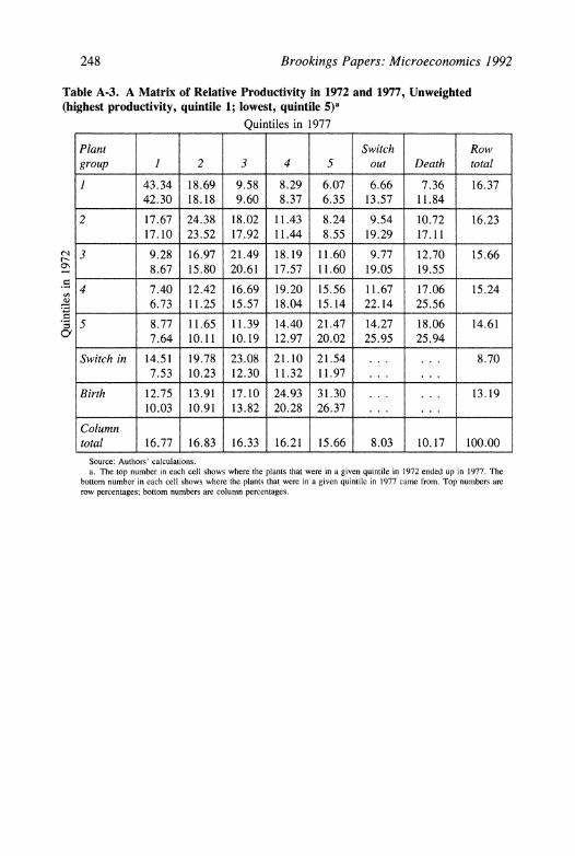
248 Brookings Papers: Microeconomics 1992
Table A-3. A Matrix of Relative Productivity in 1972 and 1977, Unweighted (highest productivity, quintile 1; lowest, quintile 5)a
Quintiles in 1977
Plant Switch Row group 1 2 3 4 5 out Death total 1 43.34 18.69 9.58 8.29 6.07 6.66 7.36 16.37
42.30 18.18 9.60 8.37 6.35 13.57 11.84
2 17.67 24.38 18.02 11.43 8.24 9.54 10.72 16.23 17.10 23.52 17.92 11.44 8.55 19.29 17.11
N 3 9.28 16.97 21.49 18.19 11.60 9.77 12.70 15.66 8.67 15.80 20.61 17.57 11.60 19.05 19.55
4 7.40 12.42 16.69 19.20 15.56 11.67 17.06 15.24 X2 6.73 11.25 15.57 18.04 15.14 22.14 25.56
5 8.77 11.65 11.39 14.40 21.47 14.27 18.06 14.61 7.64 10.11 10.19 12.97 20.02 25.95 25.94
Switch in 14.51 19.78 23.08 21.10 21.54 ... . . . 8.70 7.53 10.23 12.30 11.32 11.97 . . . ...
Birth 12.75 13.91 17.10 24.93 31.30 . .. . . . 13.19 10.03 10.91 13.82 20.28 26.37 . . .
Column total 16.77 16.83 16.33 16.21 15.66 8.03 10.17 100.00
Source: Authors' calculations. a. The top number in each cell shows where the plants that were in a given quintile in 1972 ended up in 1977. The
bottom number in each cell shows where the plants that were in a given quintile in 1977 came from. Top numbers are row percentages; bottom numbers are column percentages.
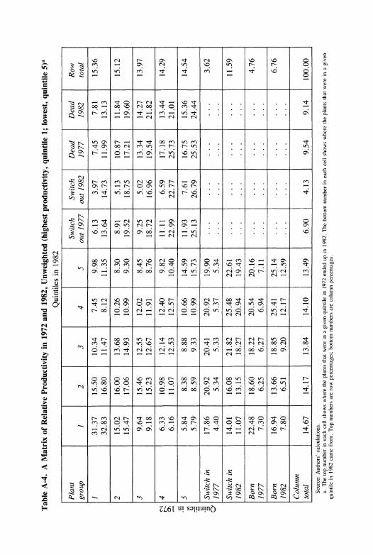
Table
A-4. A
Matrix of
Relative
Productivity in
1972
and
1982,
Unweighted
(highest
productivity,
quintile 1;
lowest,
quintile
5)a
Quintiles in
1982
Plant
Switch
Switch
Dead
Dead
Row
group
1
2
3
4
5
out
1977
out
1982
1977
1982
total
1
31.37
15.50
10.34
7.45
9.98
6.13
3.97
7.45
7.81
15.36
32.83
16.80
11.47
8.12
11.35
13.64
14.73
11.99
13.13
2
15.02
16.00
13.68
10.26
8.30
8.91
5.13
10.87
11.84
15.12
15.47
17.06
14.93
10.99
9.30
19.52
18.75
17.21
19.60
3
9.64
15.46
12.55
12.02
8.45
9.25
5.02
13.34
14.27
13.97
9.18
15.23
12.67
11.91
8.76
18.72
16.96
19.54
21.82
c
4
6.33
10.98
12.14
12.40
9.82
11.11
6.59
17.18
13.44
14.29
6.16
11.07
12.53
12.57
10.40
22.99
22.77
25.73
21.01
5
5.84
8.38
8.88
10.66
14.59
11.93
7.61
16.75
15.36
14.54
5.79
8.59
9.33
10.99
15.73
25.13
26.79
25.53
24.44
Switch in
17.86
20.92
20.41
20.92
19.90
.
.
.
.
.
.
.
.
.
.
.
.
3.62
1977
4.40
5.34
5.33
5.37
5.34
.
.
.
.
.
.
.
.
.
Switch in
14.01
16.08
21.82
25.48
22.61
...
.
|
.
.
.
.
.
..
11.59
1982
11.07
13.15
18.27
20.94
19.43
.
.
.
.
.
.
.
.
.
...
Born
22.48
18.60
18.22
20.54
20.16
.
.
.
.
.
.
.
.
.
.
.
.
4.76
1977
7.30
6.25
6.27
6.94
7.11
.
.
.
.
.
.
.
...
.
...
Born
16.94
13.66
18.85
25.41
25.14
.
.
.
.
.
.
.
.
.
.
.
.
6.76
1982
7.80
6.51
9.20
12.17
12.59
j . . .
.
..
.
..
...
Column total
14.67
14.17
13.84
14.10
13.49
6.90
4.13
9.54
9.14
100.00
Source:
Authors'
calculations.
a.
The
top
number in
each
cell
shows
where
the
plants
that
were in a
given
quintile in
1972
ended up in
1982.
The
bottom
number in
each
cell
shows
where
the
plants
that
were in a
given
quintile in
1982
came
from.
Top
numbers
are
row
percentages;
bottom
numbers
are
column
percentages.

Comments and Discussion
Comment by Timothy Bresnahan: This paper did report all 6,000 numbers, leading to somewhat different problems for discussants. Let me say, first, that it is a useful paper. In my lexicon that is high praise. Almost all the tables are about deviations, in any particular year, of plant-level productivity from industry average productivity that year. The paper reports both the static shape and the dynamic movement of that distribution in different industries, which strikes me as an extremely useful thing for analysts of productivity to do.
When I started to get comments ready, I found myself not making any criticisms whatsoever, but restating pieces of the paper in radically different language. I think it will be helpful for me to first say where the differences in language came from and then to pick a small subset of the results and try to translate back and forth a bit.
Think of productivity studies as a big house. The first language is spoken by the people who live on the roof of the house. They study aggregate productivity growth in the whole economy, increasing the well-being of the whole economy, and all that. The other language is spoken by people in the cellar who study particular technologies, maybe in particular plants. They are interested in particular technologies as they are chosen by particular managers in their individual competitive business growth and technical circumstances. "Plant" is even too ag- gregate for most of these people. "Cells" is how they think.
This paper fits into the gap between the roof of this house and the cellar because it analyzes microdata on lots of plants at lots of times. But the language of the paper is very much the language of the roof. We begin with the aggregate production function. Since we use micro-
250

Martin Neil Baily, Charles Hulten, and David Campbell 251
data, it happens to be a disaggregated production function. We decom- pose. We chase the residual for a while. It turns out the residual is still there when we are done chasing it.
And having chased the residual down to the plant level and examined its movement and thought about it, we invoke Kim Clark. Kim had his life changed, as he puts it, by exactly this finding: namely, that there is an enormous variety in productivity across plants, even within the same firm and making apparently the same thing, and that this variety appears to be persistent. We start attaching theoretical explanations like that one to the nature of the movements in the productivity and over time at the plant level.
In this house I am a cellar dweller. No Al Davis here. I think I can dramatize the difference in language between these authors and my own natural language. Much of the analysis is in five industries (motor vehicles, motor vehicle parts, construction equipment, computing equipment, and ball and roller bearings) selected by the authors because most plants produce "a single" product. I agree in a statistical sense, but not in an analytical one. We are talking about cars, cranes, car- buretors, and computers.
Even at the ball bearing plants, the biggest problem for a ball bearing manufacturing manager is the turnover of the hundreds of different models that they make. I think of these as enormously product- differentiated industries. I think of the things that go on in their tech- nical, competitive, and business-cycle runs as being things that are driven by variety-to use Clark's language again-in the mission of each plant, as much as variety in the competence of managers within each plant.
Having said how to do the translation, let me talk for a couple of seconds about the industries on this list that I understand, which are really cars and computers, and how I would have talked about the tables that came from this paper. Let me remind you that this is an elaborate agreement with the authors of this paper, a translation to a different language.
How do you make money in cars or computers? Well, there are certain commonalities in those two industries. Much of decisionmaking is about product type. Most of the costs, at least in the plant, that go with any particular product type have a big element of commitment in the one-year run.

252 Brookings Papers: Microeconomics 1992
The way you make money in the car business is to design a hot car. Now what is a hot car? Some things are just intrinsic to that business, like fads. Had you designed the Miata, you would now be rich, if you got any cut of it.
On the other hand, there are great big competitive and business-cycle forces at work that determine the size of output per unit input, a big driver for productivity at the plant level. What are those forces? Well, did you happen to design a small car just before the price of fuel went up or just before the price of fuel went down? Did you happen to roll out a whole new design just as the aggregate economy turned up or just as the aggregate economy turned down?
Plants in the United States in the car industry took three huge hits early in the study period at hand. They took an international competition hit. They took a hit, especially in the 1970s, from a dramatic change in the nature of the business cycle (particularly that it came to have big prices of fuel associated with it), and they took a regulatory hit. All of these hits tended to make obsolete the product and process knowledge that were valuable assets in place in these plants at this time.
Now we saw a period of very rapid productivity growth in that industry over the sample period of this study. The industry was getting back up to scratch from where it had been when it started. My point is that motor vehicles, like any industry, are not just a microcosm for a "typical" industry or even a typical technology-intensive durable goods industry. The forces driving the data in motor vehicles are par- ticular, and this should influence the way we use industry-specific data to illuminate broad analytical themes.
The story in computers is only a little bit different. Again firms take large bets on product types. There are fad-like forces, called standards, and other economic and international competitive forces that enor- mously affect plant-level productivity in the three- to five-year run. Inputs are largely committed to any particular venture, the size of output being determined by competitive and market forces.
Again the fact of product differentiation matters not because there should be a hedonic quality correction, but because it changes your view of the sources of manufacturing productivity shocks at the plant level.
How does this lead to the kind of results that we are seeing? Well,

Martin Neil Baily, Charles Hulten, and David Campbell 253
one of the interesting results here is that, in the industries with growing productivity over time, and those are the two that I picked out of the five, there is a lot more variety in total factor productivity (TFP) at any point in time. Those two industries happen to be ones with good solid reasons why there were enormous varieties in TFP at plant level. There were good reasons why different firms took different bets, not so much on the capability of plants-I am not sure I would say that, although that's a big deal in automobiles-but on the mission of different plants. Some of those missions turned out to be persistently high volume and, therefore, high-productivity ones; others turned out to be persistently lower volume or even failure ones.
Why change this language? Why change the language to one that emphasizes the conditions of competition or the conditions of technol- ogy in particular industries? Why sit in the cellar and look up, rather than sit on the roof and look down? I think it helps a lot in thinking about the representativeness of any particular subset of industries for telling us about the economy as a whole. The paper didn't emphasize this, but a lot of the findings, as they are related to policy, are very Porteresque. The authors like domestic competition. They think it is exactly the way to get lots of improvements in productivity and to gain competitiveness. They call competitiveness productivity; I call pro- ductivity competitiveness.
How general are the results from any particular set of industries? It is hard to answer that if you have stood on the roof and looked down and treated each plant as if it were the neoclassical-meaning, in this particular usage, know-nothing-production function of a whole econ- omy. But if you stand at the bottom and look up, you can think about whether the industries in your particular sample generalize out to the whole rest of the economy in the way their technical conditions and their competitive conditions go.
I think, at least with regard to the growing industries here, the pro- ductivity growing industries, that you could put together a pretty good story that does sound Porteresque. Indeed, it was the good features of the decentralized, competitive, let-a-thousand-flowers-bloom approach to the U.S. technology economy that was at work here and working quite effectively. The mechanism for it has little to do with managerial excellence, however. And all of that motion up and down within in-

254 Brookings Papers: Microeconomics 1992
dustry productivity distribution, that tendency of dramatic falls in reces- sions to explain a lot of the downturn, is completely consistent with that. So . . . I said this would be an elaborate agreement.
The paper also provides a regression analysis of productivity, which offers another opportunity for cellar to roof communication. In tables 8 and 9 the authors present an analysis that begins to illuminate, among other questions, the direction of causality between productivity and wages. Either causal story is interesting and important. Let me begin my query in econometric language. The errors in the two equations could be correlated with the causation running the other way. That could lead to an artificially high coefficient on the wage, even if there was no reverse causation. Suppose, for example, there was something driving both high wages and high productivity, like having a good mission for this particular plant. Why should such events be uncorre- lated with the instruments?
I am troubled, especially within industry, by the interpretative lan- guage here. What is the natural experiment that makes some plants have high wages that might cause productivity? If we follow the instruments, they are located in high-wage kinds of places. This seems to beg the question of industrial location. The theory that worker quality is useful is stuck with a pretty sorry story for its instruments; plants in high- wage places are compelled to pay more, so they have higher quality workers. The regression then asks whether they have higher produc- tivity; when this natural experiment fails to reveal that they do, the paper concludes against the worker-quality theory and for the "rents" theory. I simply do not see why the natural experiment corresponds in any meaningful way to what we would like to know about the worker- quality question. The policy question is whether we could get produc- tivity growth by fixing the school system. The fact reported is that moving all the plants to New York (a high-wage place) would not raise productivity.
Looking at table 8, I was struck by the relationship between size within industry and productivity. When Martin Baily said that he had allowed for increasing returns, that means he allowed for coefficients on inputs, which do not sum to one. We get a size-within-industry effect, which is above and beyond that and which seems to persist here.
One of the striking things to me was how much bigger that was at the 1977 peak than at the 1982 trough. Again, I think that this might

Martin Neil Baily, Charles Hulten, and David Campbell 255
be picking up-that is, size-within-industry-transitory shocks to either the mission or the capability of individual plants. If that is right, and if those are worse at the peak than at the trough, that's a really interesting fact, as are the other 5,999.
Comment by Richard E. Caves: The productivity-growth experience of industries' individual plants is an important and useful line of re- search. As Zvi Griliches pointed out, we once thought that access to microeconomic data on individual producers would yield us samples from homogeneous populations of decisionmakers; instead hetero- geneity persists unchecked, forcing us to consider the mechanisms that make it persist and the implications that it holds for patterns of resource allocation and their adjustment.
The authors' efforts complement those of other researchers to fill in the picture of how an industry's productivity changes over time with turnovers of the positions of incumbent plants and those that enter and exit. Indeed, with their analysis covering all the refined data available for these industries at the Census Bureau, there is little more to ask by way of evidence on these changes. Nonetheless, one addition would do much to raise the comprehensiveness of the analysis: including changes in control (mergers, buyouts) in the transition matrices. The study's methodology of transition matrices would be more attractive if it could embrace transitions involving changes in control. As the authors note, Frank Lichtenberg and Donald Siegel found that changes in control are on average productive when evaluated over all types of control changes and plant sizes. John Baldwin confirmed this for Canada and also found that the productivity and prevalence of control changes and entry and exit turnover vary markedly among industries. Some industries-char- acterized by the importance of intangible assets (sales-promotion out- lays, research and development) and high levels of concentration and multinational activity-exhibit extensive and productive changes in control and rather less exit/entry turnover; the complement of industries without these traits relies more on entry/exit turnover for productivity gains.1 The advantage of including transitions associated with control changes is not only that they are known to be important for productivity gains but also because their importance varies markedly with the in-
1. See Baldwin and Gorecki (1990); and Baldwin and Caves (1991).

256 Brookings Papers: Microeconomics 1992
dustry's structure. Correspondingly, the Canadian evidence suggests that the contribution of entry and exit to productivity improvement is much greater in some industries than is suggested by the low mean value found in this study.
Relation to Research on Technical Efficiency and Productivity Dispersion
As context for this analysis of plant productivity over time, I shall refer to an extensive investigation, in which I have been engaged, that analyzes the dispersions of productivity levels of plants in an industry at a point in time by employing the stochastic frontier production func- tion to estimate the gap between average and best-practice productivity for plants in each industry, and then tests hypotheses about the inter- industry variance of these levels of estimated (in)efficiency. One study by Richard Caves and David Barton (CB) deals with U.S. manufacturing industries; the other by Caves and Associates (C&A) covers Great Brit- ain, Canada, Australia, Japan, and Korea, and it includes some evidence on variations over time in the efficiency distributions of plants in each industry.2 I shall also draw on a forthcoming study by Baldwin that uses panel data on all Canadian manufacturing establishments to address questions closely similar to those pursued in this paper.3
All of this evidence is quite congenial to the authors' finding that plant productivity variations over time largely represent some combi- nation of two models: random shocks to plants' productivity levels and persistent intercept differences in those levels. The results of CB and C&A are supportive in the following ways.
First, the dispersion of plants' efficiency levels depends significantly on a number of structural and organizational factors that vary little over time. The structural factors include product differentiation and the ex- istence of heterogeneous local markets. Organizational factors include the prevalence of trade union organization and the intensity of com- petition. This finding is consistent with the authors' evidence that the
2. Caves and Barton (1990); and Caves and Associates (1992). 3. Baldwin (forthcoming).

Martin Neil Baily, Charles Hulten, and David Campbell 257
dispersion of plants' productivity levels shows a good deal of stability, especially among the most productive plants.
Second, the studies reported by C&A found evidence for each country that industrywide disturbances such as unanticipated demand changes and the occurrence of innovations tend to expand the dispersion of productivity levels, although what source of disturbance proves statis- tically significant varies from country to country. This pattern is con- sistent with the importance assigned by the authors to random shocks to plants' productivity levels.
Third, C&A provided a little evidence on the variation of efficiency over time in two countries, Great Britain and Korea. For both countries we know that estimated efficiency for the typical industry varies a good deal from year to year, but it typically vibrates randomly around a stationary mean. For Britain we were able to test hypotheses about factors that affect this vibration. As expected, it increases with the incidence of disturbances to the industry and decreases with factors that should govern the speed of plants' adjustments to disturbances.
Fourth, several of Baldwin's conclusions agree with the main findings of Baily, Hulten, and Campbell. Baldwin also noted the occurrence of considerable regression to the mean and found strong evidence that industry productivity gains depend importantly on the tendency for plants with increasing relative productivity to raise their share of ac- tivity. Following each plant's position in the productivity dispersion, he observed that average annual rates of change decline with the number of years for which the plant is observed, confirming both the role of random shocks and the existence of sustained trends in the positions of individual plants. I believe that his evidence indicates a greater role for plant turnover (entry/exit) in raising productivity than does this paper, but that impression may stem from Baldwin's use of a 10-year interval for the analysis of changes rather than a shorter one, especially since the paper by Baily, Hulten, and Campbell finds that surviving entrants' productivity levels catch up slowly to their incumbent rivals'.
Fifth, the authors conclude that a vintage model has little power to explain the behavior of plants' productivity growth rates. On the con- trary, CB found that an industry's apparent efficiency decreases with its dispersion of capital vintages (equipment not structures). In an earlier study T. Y. Shen followed individual plants through the productivity

258 Brookings Papers: Microeconomics 1992
distribution, noting that a given plant tends to slip downward until it is either renewed or exits.4 The authors may draw too-confident con- clusions from their finding of the symmetry of changes in plants' po- sitions in the productivity distribution. Given the existence of copious factors supporting a long-run dispersion in productivity levels, it is not obvious that substantial vintage effects are inconsistent with apparently symmetrical patterns of change in the distribution. Following the in- dividual plant over time is a more direct way to get at vintage effects.
Besides these points of contact in the substantive conclusions, some questions arise about the consistency of my and their conclusions. Baily, Hulten, and Campbell mention (without indicating what test was em- ployed) that they failed to find in their 23 industries the negative skew- ness used to infer technical inefficiency by means of the stochastic frontier production function. For the United States CB found negative skewness in four-fifths of all manufacturing industries, a prevalence regarded as distinctly comforting for that methodology. The other coun- try studies reported in C&A, however, found no such predominance, even though the interindustry determinants of technology efficiency (in those industries for which it could be measured) generally showed good agreement with the findings for the United States. Furthermore, a re- peated incidental finding in the studies of industrial efficiency was that exogenous factors explaining technical efficiency-inferred from the third moment of the residuals from the production function-tend strongly to be associated with the dispersion of plants' productivity levels-the second moment-as well. We remain quite puzzled by this close par- allel, which has no obvious theoretical basis.
One substantive conclusion stressed by CB was the negative asso- ciation between an industry's efficiency and the extent of enterprise- level diversification, especially in the form of control of an industry's plants by firms based in other industries. Baily, Hulten, and Campbell conclude, however, that a plant' s efficiency increases with the efficiency of whatever other manufacturing plants are operated by the same firm. The existence of such a firm effect is consistent with what most inves- tigators working with the Federal Trade Commission's Line of Business data have concluded. This finding, however, does not make the im- portant distinction between plants in the same (or closely related) in-
4. Shen (1968); also see F0rsund and Hjalmarsson (1987).

Martin Neil Baily, Charles Hulten, and David Campbell 259
dustry and widely diversified plants, nor do the dummy variables for plant ownership status utilized by Baily, Hulten, and Campbell sort this out. Researchers such as Birger Wernerfelt and Cynthia Montgomery reported quite different performance levels for closely focused and widely diversified companies.5 The analysis at hand could be pushed farther to respond more fully to this issue.
Finally, Baily, Hulten, and Campbell as well as CB encountered the problem of wildly noncredible values appearing in Census Bureau rec- ords for individual plants. This was a vexing problem for CB, whose research methodology was thought sensitive to accurate decisions about excluding bad data while retaining all observations on plants that truly are either very efficient or very inefficient. CB 's resources did not permit much testing of the sensitivity of their results to different data-editing rules, although other contributors to C&A found their results robust to alternative ways of handling dubious data. Baily, Hulten, and Campbell face the same problem, and I hope that they can be systematic about their data-editing rules and test the sensitivity of their results to different choices about inclusion or exclusion.
Interindustry Differences in Plant Productivity Growth Patterns
At this stage in their research, the authors concentrate on average patterns in the industries that they cover. They do remark upon sundry differences in those industries' underlying structures. I believe that the alternative patterns of plant productivity growth on which they focus may be present to markedly different degrees in various industries, making some degree of interindustry comparative analysis a high prior- ity. The case can be made in many ways, one being by reference to the emphasis assigned by the authors to both the stability of the positions of high-productivity plants and the force of their regression to the mean. One cannot determine "how stable is stable," but one can test hy- potheses in cross-section about what determines persistence or change. Such a procedure could be applied to various outputs of their analysis, such as the dispersion of plants' rates of productivity growth and the proportional importance of share turnover or of entry/exit for overall productivity growth.
5. Wernerfelt and Montgomery (1988).

260 Brookings Papers: Microeconomics 1992
Capital vintage effects supply an obvious example. Many industries are not very capital intensive, and others may use capital that is not subject to putty-clay effects. The evidence cited earlier, however, makes it clear that vintage effects are important for some industries, and their importance in the present sample is not ruled out by the tests reported in the paper.
Another example is the effect of variations in the aggregate growth rate of a market on the growth of productivity. The high correlation between these is well known (Verdoorn's Law), but its basis in indi- vidual decision units has been little explored. Baily, Hulten, and Camp- bell present one result that is intriguingly different: conditions of recession exact more costs in productivity by pulling plants down the productivity distribution. The reverse effect is evident in the subsequent recovery. How strong this pull is and where it works most strongly could be analyzed in cross-section as could the rate of productivity improvement of entrants relative to the market's growth rate (and the amount of turnover in the productivity positions of incumbents).
The authors also mention the role of competitive disturbances, such as large infusions of foreign investment into a U.S. industry. Dynamic competitive processes and changes in efficiency are surely associated. For example, Baldwin found that changes in seller concentration (that is, the top four firms, and in either direction) are related to greater than proportional increases in share turnover among all units competing in the market. Interindustry analysis is thus inviting for isolating the re- lation between competition in a dynamic sense and productivity growth.
Finally, some industries simply may not fit well into the authors' analytical framework. They should either be shelved or recognized for their differences. The computer industry that they mention is a case in point. Consider the set of industries in which a plant's revenue pro- ductivity depends little on the efficiency of plant-level production pro- cesses and strongly on the success of the firm in innovating or adapting its products. What appears as productivity performance in the plant then simply reflects the firm's success (or lack) in innovation. It is not obvious that the resulting pattern should be pooled with those of in- dustries in which plant-level productivity reflects process efficiency and improvements in the inputs. It also becomes plausible that plants ap- pearing highly productive at the start of a period might slip badly, or

Martin Neil Baily, Charles Hulten, and David Campbell 261
even exit, not from any loss of physical efficiency but because buyers' willingness to pay for their products has evaporated.
Although the authors are not awash with degrees of freedom in the interindustry dimension, the very fact that their industries were chosen for representativeness and diversity rather than for similarity sets the scene for a serious effort along these lines.
Policy Implications
The paper is not long on policy implications, but I shall note two areas in which a bit more caution might be appropriate. One concerns the inference that high wages (paid to skilled labor) cause high pro- ductivity among entrants while for incumbents the reverse causation seems important. That the sample includes only successful entrants might be important here; some evidence suggests that entrants face greater variance of success in activities that require the assembly of a complex team of skilled specialists, and so the productivity achieved by the successful entrants might be offset by losses run by the failures.
The other relates to the plaudits offered to well-managed firms. Aside from the issue of diversification and firm-level productivity mentioned earlier, there is a question of the persistence of firm-specific differentials over time. How persistent are firm-specific productivity differentials? Are the practices of firms with positive revenue-productivity advantages replicable by competitors, and if not, why not? What are the market- structure correlates of this persistence? These issues, which lie within gunshot of the authors' data base, need consideration before the study's implications for business management are clear.
Authors' Response: Martin Bailey, Charles Hulten, and David Camp- bell responded to Timothy Bresnahan's comments, noting that the re- sults in the paper had been extended to 23 industries, not just the 5 industries that were the subject of the earlier work.
General Discussion: Robert Hall suggested there were problems in comparing Census data on single-plant firms with data on multiplant firms because of omitted inputs. Headquarters costs, such as advertising

262 Brookings Papers: Microeconomics 1992
or administrative costs, would likely be included as inputs for a plant from a single-plant firm (since headquarters would often be on-site), but not for a plant from a multiplant firm. Hall also suggested that, in general, headquarters costs tend to be booked in larger plants, making it appear that there are diminishing returns to scale when this is, in fact, not the case. Frank Lichtenberg said that it should be possible to use available Census data to impute omitted inputs, and Martin Baily pointed to the regression results in the paper showing only small dif- ferences in productivity between single-plant firms and plants that were part of multiplant firms.
Peter Pashigian wondered about the overall effect of central admin- istration on plant productivity. He suggested that it was inappropriate to regard a multiplant firm as simply a collection of independent plants. He wanted to see a statistical test to support the idea that central ad- ministration must be having some common effect over the plants it operates.
Peter Reiss said that a joint distribution of productivity changes could be done using nonparametric statistical techniques. Reiss claimed that differences in joint distributions across industries could be examined with these techniques. Regarding plant characteristic regressions, Reiss suggested that the authors examine two different weighted regressions: the first based on fixed shares, weighting the observations by share of output, and the second based on output share changes, weighting by total factor productivity. Reiss said that these regressions would allow the authors to unpack their two-level decomposition at the plant level.
Ernst Berndt wondered why the authors used only production labor in their wage productivity equations, when the share of nonproduction labor-even excluding central office employees-probably exceeds 40 percent.
Robert Hall noted that plant productivity often falls as a result of a national or regional drop in demand since firms reduce output but retain overhead labor. He suggested that the authors must deal with this tem- poral effect on productivity more substantially.
Richard Nelson was interested in seeing the authors break down their productivity story industry by industry to highlight features that differ by industry. From his own work, he noted that in some industries technical change and productivity growth seemed to be generated in- ternally within existing firms, giving a considerable advantage to in-

Martin Neil Baily, Charles Hulten, and David Campbell 263
cumbency, whereas in other industries new technology was coming in from the outside, suggesting more possibilities for firm movement within the productivity distribution.
John Haltiwanger suggested that examination of vintage and age effects requires a more detailed characterization of plant age. He sug- gested using more exact data about plant age than just block intervals such as "zero to five years old." Based upon work that he has done with plant-level data, he noted that there are considerable differences in the behavior of one-year-old and five-year-old plants. Very young plants (one to two years old) exhibit more job turnover, have a much higher probability of failure, and also have higher net growth rates than do plants five to six years old. These results suggest that selection and learning models are important for understanding age effects in plant- level dynamics but that much of the action is in the first few years of a plant's existence.
Ariel Pakes stressed the importance of not dropping outliers when examining a productivity distribution. He said that much of the move- ment in the productivity distribution over time is attributable to firms that are at any one time on the tail of the distribution.
Lichtenberg wondered if it was more useful to examine productivity at the firm level rather than at the plant level. He noted that when some firms expand, they do not increase the size of their existing establish- ments but instead add new ones. This kind of effect on productivity must be captured at the firm level.
Frank Wolak was interested in more information about the variability of productivity at the plant level. In particular, he wondered how spe- cialization and plant age affected variability of productivity.
Bronwyn Hall wanted to see more data about the effect of foreign ownership on productivity. Hall said that if one could imagine that foreign investors were not rent sharing but instead were interested in pursuing a higher equilibrium, with higher wages and productivity, it would be important to try to distinguish these foreign owners in the regressions.

264 Brookings Papers: Microeconomics 1992
References
Abernathy, William J., Kim B. Clark, and Alan M. Kantrow. 1983. Industrial Renaissance: Producing a Competitive Future for America. New York: Basic Books.
Baldwin, John R. forthcoming. The Dynamics of the Competitive Process. New York: Cambridge University Press.
Baldwin, John R., and Paul K. Gorecki. 1990. "The Contribution of the Competitive Process to Productivity Growth: The Role of Firm and Plant Turnover." Research Paper Series 28. Ottawa: Statistics Canada.
Baldwin, John R., and Richard E. Caves. 1991. "Foreign Multinational En- terprises and Merger Activity in Canada." In Leonard Waverman, ed., Cor- porate Globalization Through Mergers and Acquisitions, pp. 89-122. Calgary: University of Calgary Press.
Bartelsman, Eric J., and Phoebus J. Dhrymes. 1992. "Productivity Dynamics: U. S. Manufacturing Plants, 1972-1986." Discussion Paper CES 92-1. Center for Economic Studies, Bureau of the Census. February.
Bregman, Arie, Melvyn Fuss, and Haim Regev. forthcoming. "The Production and Cost Structure of Israeli Industry: Evidence from Individual Firm Data." Journal of Econometrics.
Caves, Richard E., and Associates. 1992. Industrial Efficiency in Six Nations. Cambridge: MIT Press.
Caves, Richard E., and David R. Barton. 1990. Efficiency in U. S. Manufac- turing Industries. Cambridge, Mass.: MIT Press.
Christensen, L. R., D. Cummings, and D. W. Jorgenson. 1981. "Relative Productivity Levels, 1947-1973: An International Comparison." European Economic Review 16 (May):61-94.
Davis, Steve J., and John Haltiwanger. 1991. "Wage Dispersion Between and Within U. S. Manufacturing Plants, 1963-86." Brookings Papers on Eco- nomic Activity: Microeconomics, 1991: 115-200.
Dertouzos, Michael L., Richard K. Lester, and Robert M. Solow. 1989. Made in America: Regaining the Productive Edge. Cambridge, Mass.: MIT Press.
Dhrymes, Phoebus J. 1990. "The Structure of Production Technology: Evi- dence from the LED Sample I." In Bureau of the Census Proceedings of the 1990 Annual Research Conference. Washington, D. C.: Department of Commerce.
Diebold, Frank X., and Glenn D. Rudebusch. forthcoming. "Have Postwar Economic Fluctuations Been Stabilized?" American Economic Review.
Doms, Mark E. 1992. "Estimating Capital Efficiency Schedules Within Pro- duction Functions." Discussion Paper CES 92-4. Center for Economic Stud- ies, Bureau of the Census. April.
Dunne, Timothy. 1991. "Technology Usage in U. S. Manufacturing Indus-

Martin Neil Baily, Charles Hulten, and David Campbell 265
tries: New Evidence from the Survey of Manufacturing Technology." Dis- cussion Paper CES 91-7. Center for Economic Studies, Bureau of the Census. November.
Dunne, Timothy, and Mark J. Roberts. 1990. "Wages and the Risk of Plant Closings." Discussion Paper CES 90-6. Center for Economic Studies, Bu- reau of the Census. July.
Dunne, Timothy, Mark J. Roberts, and Larry Samuelson. 1988. "Patterns of Firm Entry and Exit in U. S. Manufacturing Industries." Rand Journal of Economics 19 (Winter): 495-515.
Ericson, Richardson, and Ariel Pakes. 1989. "An Alternative Theory of the Firm and Industry Dynamics." Discussion Paper 445. Columbia University. September.
F0rsund, Finn R., and Lennart Hjalmarsson. 1987. Analyses of Industrial Structure. A Putty-Clay Approach. Stockholm: Institute for Economic and Social Research.
Friedman, Milton. 1937. "The Use of Ranks to Avoid the Assumption of Normality Implicit in the Analysis of Variance." Journal of the American Statistical Association 32:675-701.
. 1940. "A Comparison of Alternative Tests of Significance for the Problem of m Rankings." Annals of Mathematical Statistics 38:867-77.
Gort, Michael, Byong-Hyong Bahk, and Richard A. Wall. 1991. "Decom- posing Technical Change." Discussion Paper CES 91-4. Center for Eco- nomic Studies, Bureau of the Census. May.
Griliches, Zvi. 1979. "Issues in Assessing the Contribution of Research and Development to Productivity Growth." Bell Journal of Economics 10 (Spring):92-116.
Griliches, Zvi, and Haim Regev. forthcoming. "Firm Turnover and Produc- tivity Growth in Israeli Industry: 1979-1988." Cambridge, Mass.: National Bureau of Economic Research.
Griliches, Zvi, and Jacques Mairesse. 1983. "Comparing Productivity Growth: An Exploration of French and U. S. Industrial and Firm Data." European Economic Review 21 (March/April):89- 128.
Griliches, Zvi, and Vidar Ringstad. 1971. Economies of Scale and the Form of the Production Function: An Econometric Study of Norwegian Manufac- turing Establishment Data. Amsterdam: North-Holland.
Hall, Robert E. 1988. "The Relation Between Price and Marginal Cost in U. S. Industry." Journal of Political Economy 96 (October):921-47.
. 1990. "Invariance Properties of Solow's Productivity Residual." In Peter Diamond, ed., Growth, Productivity, Unemployment: Essays to Cel- ebrate Bob Solow's Birthday. Cambridge, Mass.: MIT Press.
Hart, P. E., and S. J. Prais. 1956. "The Analysis of Business Concentration: A Statistical Approach." Journal of the Royal Statistical Society, pt. 2, vol. 119:150-91.

266 Brookings Papers: Microeconomics 1992
Hayes, Robert H., Steven C. Wheelwright, and Kim B. Clark. 1988. Dynamic Manufacturing: Creating the Learning Organization. New York: The Free Press.
Hazilla, Michael, and Raymond J. Kopp. 1987. "Establishment-Level Data for Econometric, Engineering, and Policy Analysis: Phase I." Discussion Paper OE87-03. Washington, D.C.: Resources for the Future. January.
Jovanovic, Boyan. 1982. "Selection and the Evolution of Industry." Econo- metrica 50 (May):649-70.
Katz, Lawrence, F., and Lawrence H. Summers. 1989. "Industry Rents: Ev- idence and Implications." Brookings Papers on Economic Activity: Mi- croeconomics, 1989: 209-75.
Leham, E. L., and H. J. M. D'Abrera. 1975. Nonparametrics: Statistical Methods Based on Ranks. San Francisco: Holden-Day.
Lichtenberg, Frank R., and Donald Siegel. 1987. "Productivity and Changes in Ownership of Manufacturing Plants." Brookings Papers on Economic Activity 3:643-73.
Lucas, Robert E., Jr. 1978. "On the Size Distribution of Business Firms." Bell Journal of Economics 9 (Autumn):508-23.
McGuckin, Robert H. 1989. "Longitudinal Economic Data at the Census Bu- reau: A New Data Base Yields Fresh Insights on Some Old Issues." Pro- ceedings of the Statistics Canada Symposium on Analysis of Data in Time. October.
McGuckin, Robert H., and George A. Pascoe, Jr. 1988. "The Longitudinal Research Database: Status and Research Possibilities." Survey of Current Business 68 (November): 30-37.
Mairesse, Jacques, and Zvi Griliches. 1990. "Heterogeneity in Panel Data: Are There Stable Production Functions?" In Paul Champsaur, ed., Essays in Honor of Edmond Malivaud. Vol. 3, Empirical Economics. Cambridge, Mass.: MIT Press.
Nelson, Richard R., and Sidney G. Winter. 1978. "Forces Generating and Limiting Concentration Under Schumpeterian Competition." Bell Journal of Economics 9 (Autumn):5240-48.
. 1982. An Evolutionary Theory of Economic Change. Cambridge, Mass.: Belknap Press at Harvard University.
Nguyen, Sang V., and Arnold P. Reznek. 1991. "Returns to Scale in Small and Large U. S. Manufacturing Establishments." Small Business Economics 3: 197-214.
Olley, G. Steven, and Ariel Pakes. 1992. "The Dynamics Productivity in the Telecommunications Equipment Industry." Working Paper 3977. Cam- bridge, Mass.: National Bureau of Economic Research. January.
Romer, Paul. 1990. "Endogenous Technical Change." Journal of Political Economy 98 (October): S71-S102.

Martin Neil Baily, Charles Hulten, and David Campbell 267
Scherer, F. M. 1984. Innovation and Growth: Schumpeterian Perspectives. Cambridge, Mass.: MIT Press.
Schumpeter, Josef A. 1936. The Theory of Economic Development: An Inquiry into Profits, Capital, Credit, Interest, and the Business Cycle. Cambridge, Mass.: Harvard University Press.
Shen, T. Y. 1968. "Competition, Technology, and Market Shares." Review of Economics and Statistics 50 (February):96-102.
Streitwieser, Mary L. 1991. "The Extent and Nature of Establishment-Level Diversification in Sixteen Manufacturing Industries." Journal of Law and Economics, vol. 34, no. 2, pt. 2:503-34.
Wernerfelt, Birger, and Cynthia A. Montgomery. 1988. "Tobin's q and the Importance of Focus in Firm Performance." American Economic Review 78 (March):246-50.
White, Halbert. 1980. "A Heteroskedasticity-Consistent Covariance Matrix Estimator and a Direct Test of Heteroskedasticity. " Econometrica 48 (May):817-38.