Production Scheduling and System Configuration for Capacitated Flow Lines with

Application in the Semiconductor Backend Process

by

Mengying Fu

A Dissertation Presented in Partial Fulfillmentof the Requirements for the Degree

Doctor of Philosophy

Approved April 2011 by theGraduate Supervisory Committee:

Ronald Askin, Co-ChairMohong Zhang, Co-Chair

John FowlerRong Pan

Arunabha Sen

ARIZONA STATE UNIVERSITY

May 2011

ABSTRACT

A good production schedule in a semiconductor back-end facility is critical for

the on time delivery of customer orders. Compared to the front-end process that is

dominated by re-entrant product flows, the back-end process is linear and therefore

more suitable for scheduling. However, the production scheduling of the back-end

process is still very difficult due to the wide product mix, large number of parallel

machines, product family related setups, machine-product qualification, and weekly

demand consisting of thousands of lots.

In this research, a novel mixed-integer-linear-programming (MILP) model is

proposed for the batch production scheduling of a semiconductor back-end facil-

ity. In the MILP formulation, the manufacturing process is modeled as a flexible

flow line with bottleneck stages, unrelated parallel machines, product family re-

lated sequence-independent setups, and product-machine qualification considera-

tions. However, this MILP formulation is difficult to solve for real size problem in-

stances. In a semiconductor back-end facility, production scheduling usually needs

to be done every day while considering updated demand forecast for a medium term

planning horizon. Due to the limitation on the solvable size of the MILP model, a

deterministic scheduling system (DSS), consisting of an optimizer and a scheduler,

is proposed to provide sub-optimal solutions in a short time for real size problem

instances. The optimizer generates a tentative production plan. Then the scheduler

sequences each lot on each individual machine according to the tentative production

plan and scheduling rules. Customized factory rules and additional resource con-

straints are included in the DSS, such as preventive maintenance schedule, setup

crew availability, and carrier limitations. Small problem instances are randomly

generated to compare the performances of the MILP model and the deterministic

scheduling system. Then experimental design is applied to understand the behavior

of the DSS and identify the best configuration of the DSS under different demandii

scenarios.

Product-machine qualification decisions have long-term and significant impact

on production scheduling. A robust product-machine qualification matrix is critical

for meeting demand when demand quantity or mix varies. In the second part of

this research, a stochastic mixed integer programming model is proposed to bal-

ance the tradeoff between current machine qualification costs and future backorder

costs with uncertain demand. The L-shaped method and acceleration techniques

are proposed to solve the stochastic model. Computational results are provided to

compare the performance of different solution methods.

iii

ACKNOWLEDGEMENTS

I would like to thank everyone that helped make this dissertation possible.

First, I would like to thank my committee members. I thank Dr. Ronald Askin

for being a great advisor. Without his guidance, encouragement, support, and pa-

tience, I would have never finished this dissertation. I would also like to thank my

co-advisor Dr. Muhong Zhang for her assistance. I am deeply grateful to her for the

long discussions that helped me resolve difficult optimization problems. Thanks to

Dr. John Fowler for insightful comments and suggestions at different stages of my

research and study. Thanks for Dr. Rong Pan and Dr. Arunabha Sen, who gra-

ciously agreed to serve on my committee, for their very helpful insights, comments

and suggestions at my proposal meeting.

Then, I would like to acknowledge faculty members in the School of Comput-

ing, Informatics, and Decision Systems Engineering at Arizona State University

for numerous discussions and lectures on related topics that helped me improve my

knowledge in the area.

Additionally, I appreciate the financial support from Intel that funded parts of

the research discussed in this dissertation.

Finally, I would like to thank my fellow graduate students, alphabetically: Jun-

zilan Chen, Moeed Haghnevis, Wandaliz Torres Garcia, Serhat Gul, Shrikant Jarugu-

milli, Jinjin Li, Qing Li, Paul Maliszewski, Adrian Ramirez Nafarrate, Shanshan

Wang, Liangjie Xue, Mingjun Xia, for their friendship and support throughout this

process.

Last but not least, I would like to thank my parents for supporting me to explore

my own potential. All the love and understanding they have provided me over the

years was the greatest gift anyone has ever given me.

iv

TABLE OF CONTENTS

Page

TABLE OF CONTENTS . . . . . . . . . . . . . . . . . . . . . . . . . . . . v

LIST OF FIGURES . . . . . . . . . . . . . . . . . . . . . . . . . . . . . . . vii

LIST OF TABLES . . . . . . . . . . . . . . . . . . . . . . . . . . . . . . . viii

CHAPTER 1 INTRODUCTION . . . . . . . . . . . . . . . . . . . . . . . 1

CHAPTER 2 LITERATURE REVIEW . . . . . . . . . . . . . . . . . . . . 6

2.1 Flow Shop Scheduling . . . . . . . . . . . . . . . . . . . . . . . . 6

2.2 Flexible Flow Shop Scheduling . . . . . . . . . . . . . . . . . . . . 8

2.3 Semiconductor Back-End Process Scheduling . . . . . . . . . . . . 10

2.4 Product-Machine Qualifications . . . . . . . . . . . . . . . . . . . 12

CHAPTER 3 OPTIMIZATION MODEL . . . . . . . . . . . . . . . . . . . 14

CHAPTER 4 DETERMINISTIC SCHEDULING SYSTEM (DSS) . . . . . 24

4.1 Optimizer . . . . . . . . . . . . . . . . . . . . . . . . . . . . . . . 26

4.2 Scheduler . . . . . . . . . . . . . . . . . . . . . . . . . . . . . . . 30

4.3 Parameters . . . . . . . . . . . . . . . . . . . . . . . . . . . . . . . 32

CHAPTER 5 EXPERIMENT RESULTS . . . . . . . . . . . . . . . . . . . 35

5.1 General Evaluation . . . . . . . . . . . . . . . . . . . . . . . . . . 35

5.2 Offline Optimization of the DSS Parameters with Single Objective . 37

5.3 Offline Optimization of the DSS Parameters with Multiple Objectives 42

5.4 Summary . . . . . . . . . . . . . . . . . . . . . . . . . . . . . . . 47

CHAPTER 6 STOCHASTIC MACHINE QUALIFICATION OPTIMIZA-

TION . . . . . . . . . . . . . . . . . . . . . . . . . . . . . . 50

6.1 Introduction . . . . . . . . . . . . . . . . . . . . . . . . . . . . . . 50

6.2 Problem Statement . . . . . . . . . . . . . . . . . . . . . . . . . . 52

6.3 Stochastic Machine Qualification Optimization Model (S-MQO) . . 57

v

Chapter Page

6.4 Deterministic Equivalent Formulation . . . . . . . . . . . . . . . . 58

L-Shaped Method . . . . . . . . . . . . . . . . . . . . . . . . . . . 59

Acceleration of The L-Shaped Method . . . . . . . . . . . . . . . . 63

6.5 Computational Experiments . . . . . . . . . . . . . . . . . . . . . . 67

Data . . . . . . . . . . . . . . . . . . . . . . . . . . . . . . . . . . 67

Performance of Different Solution Methods . . . . . . . . . . . . . 70

6.6 Summary . . . . . . . . . . . . . . . . . . . . . . . . . . . . . . . 75

CHAPTER 7 CONCLUSION . . . . . . . . . . . . . . . . . . . . . . . . . 76

REFERENCES . . . . . . . . . . . . . . . . . . . . . . . . . . . . . . . . . 78

APPENDIX . . . . . . . . . . . . . . . . . . . . . . . . . . . . . . . . . . . 83

A A MIXED INTEGER LINEAR PROGRAMMING MODEL FOR

GENERALIZED FLEXIBLE FLOW SHOP SCHEDULING . . . . . 84

B FUNCTIONS DEFINED IN SCHEDULER . . . . . . . . . . . . . . 90

vi

LIST OF FIGURES

Figure Page

1.1 Semiconductor Back-end Process . . . . . . . . . . . . . . . . . . . . . 2

3.1 Setup Scenarios During One Time Period . . . . . . . . . . . . . . . . 16

3.2 Inventory Update . . . . . . . . . . . . . . . . . . . . . . . . . . . . . 20

3.3 Setup Continuation . . . . . . . . . . . . . . . . . . . . . . . . . . . . 21

4.1 Deterministic Scheduling System (DSS) . . . . . . . . . . . . . . . . . 25

4.2 Discrete Event System . . . . . . . . . . . . . . . . . . . . . . . . . . 30

5.1 Solution Value Summary for Small Problem Instances . . . . . . . . . . 38

6.1 Manufacturing system description . . . . . . . . . . . . . . . . . . . . 67

6.2 Solution times of different solution methods . . . . . . . . . . . . . . . 72

vii

LIST OF TABLES

Table Page

5.1 Toy Data Size . . . . . . . . . . . . . . . . . . . . . . . . . . . . . . . 35

5.2 DSS Parameter Values . . . . . . . . . . . . . . . . . . . . . . . . . . 35

5.3 Matched Pairs Analysis of Grouped Data for Small Problem Instance

Solution Values . . . . . . . . . . . . . . . . . . . . . . . . . . . . . . 39

5.4 Solution Time Summary for Small Problem Instances (seconds) . . . . 40

5.5 Independent Variables in the Experiment Design (Single Objective) . . . 41

5.6 Design of Experiment (Single Objective) Statistical Summary . . . . . . 43

5.7 Recommended Configuration Under Each Scenario (Single Objective) . 44

5.8 Independent Variables in the Experimental Design (Multiple Objectives) 45

5.9 Responses in the Experimental Design (Multiple Objective) . . . . . . . 45

5.10 Statistical Summary of Responses (Multiple Objectives) . . . . . . . . . 46

5.11 Suggested Parameter Values (Multiple Objectives) . . . . . . . . . . . . 47

5.12 Suggested Parameter Values with Three Fixed Parameters (Multiple

Objectives) . . . . . . . . . . . . . . . . . . . . . . . . . . . . . . . . 48

6.1 Manufacturing System Description. . . . . . . . . . . . . . . . . . . . 68

6.2 Weekly Demand. . . . . . . . . . . . . . . . . . . . . . . . . . . . . . 68

6.3 Size of the deterministic equivalent of the S-MQO problem. . . . . . . . 69

6.4 Solution time comparison of different acceleration methods . . . . . . . 73

6.5 Solution quality comparison of different acceleration methods. . . . . . 74

6.6 Evaluation of different qualification matrices. . . . . . . . . . . . . . . 75

viii

CHAPTER 1

INTRODUCTION

This research addresses the production scheduling of semiconductor back-end fa-

cilities, but the proposed methods could be applied to any process that has a similar

structure. Semiconductors, also referred as integrated circuits (ICs), are contained

in many commonly used electrical and electronic devices. There are numerous elec-

trical pathways connecting to billions of transistors on the semiconductors. Those

transistors perform binary operations by either holding an electric charge or holding

little/no charge. Semiconductor manufacturing process consists of 9 main steps.

Step 1 Silicon is used to grow silicon crystals that are then sliced into wafers;

Step 2 One side of each wafer is polished, on which chips are built;

Step 3 A layer of silicon dioxide glass is grown on the polished side of the wafer;

Step 4 Photolithography is used to create a layer of circuit patterns on the chip;

Step 5 The wafer goes to the etch area where materials are removed in a series of

steps, resulting a pattern of silicon dioxide on top of the wafer;

Step 6 Through several photolithography and etch steps, subsequent layers of var-

ious patterned materials are built up on the wafer to form the multiple layers

of circuit patterns in a single chip (re-entrant product flow);

Step 7 Certain areas of the wafer are exposed to chemicals that change their ability

to conduct electricity;

Step 8 A conducting metal (usually copper) is first electro-plated on the entire

wafer surface and then polished off selectively, leaving thin lines of metal

interconnects;

Step 9 First, each chip is tested for electrical performance and sorted accordingly;

then, each chip is put into an individual package; at last, chips are tested again

to make sure they function properly.

Operations in steps 1-8 are usually called the front-end process or wafer fabrication,

and the assembly and test operations in step 9 are called the back-end process. A

typical semiconductor assembly and test facility has approximately 30 aggregated

product families, 30 nearly linear processing operations, and more than 300 ma-

chines on the floor. Orders of the same product family are grouped into lots of 1024

units. Weekly demand consists of more than a thousand lots with a throughput time

as long as a couple of weeks. As the last section of semiconductor manufacturing,

meeting customer orders on time is the most important criterion, in particularly we

desire to minimize the total tardiness. When the demand exceeds the capacity, the

priority of each lot needs to be considered. For example, confirmed customer orders

have higher priorities than internal orders based on forecast, and some order is more

profitable than others, thus assigned a higher priority. Therefore the objective of the

production scheduling in this research is to minimize the total prioritized tardiness.

Machine 1

Machine M1

Unfinishedproducts

Finishedproducts

Stage 1

Machine 1

Machine M2

Stage 2

Machine 1

Machine Mn

Stage n

Operation 1 Operation n+1Operation 2 Operation n

Figure 1.1: Semiconductor Back-end Process

2

The production system modeled in this research is shown in Figure 1.1. There

is a unique route, which is a list of sequential operations, for each product family.

The product flow in the back-end process is unidirectional, compared to the front-

end process which is dominated by reentrant operations. However, some operations

or stages could be skipped for some product families. There are unrelated parallel

machines at each stage, which can perform the same operation(s). A machine can

only process product families that it has been qualified for. The product-machine

qualification is a production system configuration decision and represented by a

two-dimensional 0-1 matrix. There could be more than one operation performed at

one stage with different sequences. The processing times for the same operation and

product family at different machines can be different, which are determined by the

machine type. There is a sequence-dependent setup when a machine switches be-

tween product families or operations. When an operation is started on a machine,

no interruption is allowed (non-preemptive scheduling). The production system

described so far can be characterized as a flexible flow shop with family-related

sequence-dependent setup times, product-machine qualification, and multiple oper-

ations at one stage. A novel mixed integer linear programming model is proposed

in this research for the medium term (e.g. several weeks) production scheduling

of the above system. It is shown in Gupta [1988] that a two-stage flexible flow

shop scheduling problem with a single machine at one stage is NP-hard. Since that

problem can be seen as a special case of the general flexible flow shop schedul-

ing problem with setup considerations, it could then be concluded that the general

flexible flow shop scheduling problem with setups is also NP-Hard. Moreover,

there are product-machine qualifications, multiple operations at one stage, and cus-

tomized constraints in the semiconductor back-end process, which are not usually

considered in the classic flexible flow shop scheduling models. Customized con-

straints include machine preventive maintenance schedules, machine engineering3

time schedules, and the availability of other resources in the manufacturing pro-

cess such as staff for setups, tools, etc. Those constraints are non-neligible in the

scheduling process, and also make the scheduling problem even more difficult. A

deterministic scheduling system is proposed to provide a sub-optimal production

schedule for real size problem instances in a short time while considering all im-

portant customized constraints in the shop floor.

In a semiconductor back-end facility, each machine needs to be configured for

the product families it will process in the future. The configuration process in-

cludes installing and testing a software program for each product on the machine.

The configuration of the production system with respect to product families is rep-

resented by the product-machine qualification matrix, which is a two-dimensional

0− 1 matrix with 1 meaning the corresponding machine qualified for the corre-

sponding product and 0 otherwise. Product-machine qualification decisions are

critical because of their long-term impact on future production scheduling. Usu-

ally not all machines are qualified for all product families in a back-end facility.

The first reason is that not all machines are technologically capable of process-

ing all products due to the fast development of new products and machines in the

semiconductor industry. The second reason is that qualifying all machines for all

products is not financially efficient. On the other hand, the product-machine qualifi-

cation should be robust enough to handle future demand with different quantities or

mix. As a result, product-machine qualification decisions are complex because of

the wide product mix, large number of machines, and demand uncertainty. In this

research, a stochastic model is proposed to to minimize product-machine qualifica-

tion cost while considering future production scheduling with demand uncertainty.

The remainder of the dissertation is organized as follows. Chapter 2 is a compre-

hensive literature review about general production scheduling, production schedul-

ing in a semiconductor back-end facility, and product-machine qualifications. In4

Chapter 3, a MILP formulation is presented and described for solving the flexi-

ble flow line scheduling problem with family-related sequence-independent setup

times, product-machine qualification, and multiple operations at one stage. This is

followed by Chapter 4, in which a deterministic scheduling system is proposed for

the semiconductor back-end operations scheduling with the ability to consider all

additional constraints and solve large problem instances in a reasonable time. In

Chapter 5, computational experiments and results are presented to show solvable

size of the MILP formulation, comparison between the DSS solutions and the op-

timal solutions for small problem instances, and the behavior of the DSS for real

size problem instances. in Chapter 6, a stochastic model and several solution meth-

ods are proposed for product-machine qualification optimization in the back-end

facility. Computational results are presented to show the comparison between the

deterministic and stochastic models as well as different solution methods of the

stochastic model. Finally, this research is concluded in Chapter 7.

5

CHAPTER 2

LITERATURE REVIEW

Literature related to our scheduling problem and production-machine qualification

optimization is reviewed in this chapter.

2.1 Flow Shop Scheduling

First, literature on flow shop scheduling problems with setup times is discussed.

A flow shop is a multi-stage production system with more than one parallel ma-

chines at each stage and all products going through the system unidirectionally, e.g.

stage 1, then stage 2, and so on. The area of flow shop scheduling has been exten-

sively studied in the past 50 years since Johnson [1954]. There are thousands of

papers about different optimal procedures and heuristics for solving the flow shop

scheduling problem and its variants. Quadt and Kuhn [2007] gave a comprehensive

review about different solution procedures of the flow shop scheduling problem.

Most optimal procedures are based on Branch & Bound and setup times are not

included in modeling. Salvador [1972] proposes a Branch & Bound algorithm that

generates a permutation schedule, e.g. the same sequence of jobs at every stage.

Brah and Hunsucker [1991] develop another Branch & Bound algorithm based

on searching the space of possible job sequences for each parallel machine stage

by stage, generating a non-permutation schedule. Brockmann and Dangelmaier

[1997], Brockmann et al. [1998] develop and improve a parallelized version of the

algorithm presented by Brah and Hunsucker [1991], speeding up the computation

by using multiple computer processors. Portmann et al. [1998] improve Brah and

Hunsucker [1991] by using a genetic algorithm to derive upper bounds during the

Branch & Bound procedure. Carlier and Neron [2000] consider all the stages si-

multaneously and generate search tree by selecting sequentially a stage and the next

job to be scheduled at that stage. Neron et al. [2001] implement the concepts of ‘en-

ergetic reasoning’ and ‘global operation’ to speed up the procedure. Harjunkoski

and Grossmann [2002] propose a algorithm that iteratively assign jobs to machines

and then sequence the jobs assigned to one machine. More detail about exact op-

timal solution procedures for flow shop scheduling problems can be found in Kis

and Pesch [2005].

However, flow shop scheduling models with exact solution procedures are usu-

ally simplified compared to the real processes, and thus difficult to be applied in a

real facility. The exact solution procedures also take a fairly long time and there-

fore could only handle small size problems within a reasonable time. As a result,

heuristics are developed to provide faster solutions (usually not optimal) or deal

with real size problem instances. Agnetis et al. [1997] propose a simple heuris-

tic to select next job from the queue using dispatching rules whenever a machine

becomes idle. Some heuristics use local search methods or metaheuristics. The dif-

ference between the two is that local search methods accept a new solution only if

it is better than current solution while metaheuristics also accept worse solutions to

avoid local optimum. Comparisons of several tabu search heuristics by Hurink et al.

[1994], Dauzere-Peres and Paulli [1997], and Nowicki and Smutnicki [1998] can

be found in Negenman [2001]. Leon and Ramamoorthy [1997] propose a different

way of applying local search in flow shop scheduling, searching neighborhood of

the input data rather than the neighborhood of the schedule. The above heuristics

solve the flowshop scheduling problem in a integrated way. Another large cate-

gory of heuristics decompose the problem based on stage or job. Stage-oriented

decomposition approaches divide the whole problem into several single stage, mul-

tiple machine scheduling subproblems. Mokotoff [2001] gives an review of single

stage multiple machine scheduling problem. Most stage-oriented decomposition

approaches are based on ‘list schedules’, introduced by Graham [1969] for single7

stage multiple machine scheduling problem. List schedules can be adapted with

standard flow line algorithm or with local search or metaheuristics, for the coordi-

nation between stages. In the first method, jobs are sequenced by the aggregated

standard flow line (a flow line with single machine at each stage) algorithm (see

Cheng et al. [2000] for an overview) for a selected stage. Then parallel machines

at that stage are considered explicitly and a machine is selected for each job us-

ing list schedules. The next stage is scheduled similarly using the job sequence

from the previous stage. See Ding and Kittichartphayak [1994], Lee and Vairak-

tarakis [1994], Guinet and Solomon [1996], Botta-Genoulaz [2000], Koulamas and

Kyparisis [2000], and Soewandi and Elmaghraby [2001] for more variants of this

method. In the latter method, local search or metaheuristics are used to create and

improve initial job sequence [Kochhar and Morris, 1987, Jin et al., 2002, Kurz and

Askin, 2004]. Job-oriented decomposition approaches schedule all jobs sequen-

tially with one job each time at all stages [Sawik, 1993, Gupta et al., 2002, Phadnis

et al., 2003].

2.2 Flexible Flow Shop Scheduling

If a flow shop is “flexible”, some products can skip some stages. Usually in a

flow shop, all the parallel machines at the same stage are identical and can only

perform one operation. However, in a semiconductor back-end facility and also

in some other factories (with very different product families), parallel machines

could belong to different machine types. Each machine type may only process a

subset of product families and has its unique processing time for each product fam-

ily. In this case, the parallel machines are called unrelated. The machines used

to test packaged chips can perform different types of tests, and there is a minor

setup time between different tests even for the same lot. Those above two char-

acteristics, product-machine qualification and multiple operations at one stage, are

8

usually not considered in the classic flexible flow shop scheduling literature. The

flexible flow shop structure is very commonly used in manufacturing industry and

thus has drawn considerable attention in scheduling research. Flexible flow shop

scheduling problems with setup times can be divided into four categories depend-

ing on what types of setup time is considered: sequence-independent or sequence-

dependent setup times, and non-batch (job based) or batch (product family based)

setup times. Sequence-dependent or batch setup times makes the scheduling prob-

lem much more difficult compared to its counterpart. Due to the complexity of

the problem, most literature on flexible flow shop with setup times focuses on de-

veloping heuristics. The flexible flow shop scheduling problem with non-batch

sequence-dependent setup times is first formulated by Liu and Chang [2000] as a

separable integer programming problem and provides a search heuristic based on

Lagrangian relaxation. The scheduling objective is minimizing earliness, tardiness,

and setup cost. The scheduling time horizon is also divided into time periods, and

all setup/processing times are measured in units of time periods. Four heuristics

for flexible flow shop scheduling with non-batch sequence-dependent setup times

are reviewed by Kurz and Askin [2004], based on lower bounds developed in the

paper. A two-stage flexible flow shop with a single machine at the first stage and

parallel uniform machines at the second stage is modeled by Huang and Li [1998]

while considering batch sequence-independent setup times. Two lower bounds and

two heuristics based on sequencing rules are proposed and tested with problems up

to 5 product families, 15 lots in each product family, and 8 machines at stage 2.

The objective is to minimize the makespan and the heuristic solutions are 20% to

60% above the lower bounds. A general flexible flow shop with batch sequence-

independent setup with grouped jobs is studied by Logendran et al. [2005] with the

objective of minimizing the makespan and a two-level group scheduling strategy

is implemented: first sequencing within the group and then sequencing the groups.9

Three different heuristic algorithms are compared using statistical experiments, in

which problems up to 7 stages, 7 product families, and 10 lots in each product fam-

ily are solved. Group technology is also considered by both Andres et al. [2005]

and Logendran et al. [2006]. A case study from a label sticker manufacturing com-

pany is provided by Lin and Liao [2003]. The manufacturing process consists of

two stages: a high speed machine requiring batch sequence-dependent setups at

the first stage, and two different types of dedicated machines with negligible setups

at the second stage. The scheduling objective is to minimize the weighted maxi-

mal tardiness. Scheduling rules based on sequencing and dispatching methods are

proposed and tested on small sized problems. Recently, metaheuristic algorithms

have been used to generate schedules for complex manufacturing systems. Ruiz

and Maroto [2006] propose a generic algorithm to solve a general flexible flow

shop scheduling with non-batch sequence-dependent setup times and machine el-

igibility. The algorithm is compared to adaptations of other metaheuristics with

problems up to 200 jobs and 20 stages. For a comprehensive up-to-date review on

scheduling problems with setup considerations, the reader is referred to Allahverdi

et al. [2008]. The product-machine qualification and setup considerations make the

problem more difficult compared to general flexible flow line scheduling problems.

2.3 Semiconductor Back-End Process Scheduling

In addition to the literature studying general flexible flow shop scheduling prob-

lems with batch setup times, research has also been done specifically for schedul-

ing in semiconductor back-end facilities. A disjunctive graph is used to model the

workcenters in a test facility in Uzsoy et al. [1991]. Computational results are pro-

vided for up to 5 lots with 15 operations. Since each lot is modeled explicitly in

this model, the problem size increases when the number of lots to be scheduled

becomes larger. This limits the implementation of the method in real time schedul-

10

ing because a semiconductor test facility usually processes thousands of lots each

week. A simulation based scheduling and optimization framework is first proposed

for the semiconductor back-end process in Sivakumar [1999]. An offline deter-

ministic simulation model is built and customized to implement scheduling rules

that try to improve cycle time, delivery, and utilization, while considering related

resource constraints and down stream work-in-process(WIP) status. In Sivakumar

and Chong [2001], a data driven discrete event simulation model is used to study the

impact of different control parameters in the current production scheduling strategy

on the cycle time distribution and throughput of a semiconductor back-end facility.

In Liu et al. [2005], a lot release strategy is developed for the semiconductor back

end facility, based on lot prioritization and capacity constraints, along with other

control mechanism such as machine loading strategy to minimize conversions. In

a more recent study Werner et al. [2006], an online simulation model for a semi-

conductor back-end facility is built, and then the lot release strategy as well as

the lot sequence on the bottleneck stages are improved using Threshold Accept-

ing. Later in Weigert et al. [2009], the same system is optimized using iterative

heuristic search strategies under multiple objectives. In Chiang et al. [2008], fuzzy

analytical hierarchy process (AHP) is introduced to the scheduling process to iden-

tify a acceptable WIP deviation level at each bottleneck operation, which is then

used to set lot priority in the scheduling process. The method is tested in a simula-

tion model with real-world data. Customer satisfactory and on-time delivery are the

main objective in this paper. In Jarugumilli et al. [2008], an optimization-simulation

framework and a mixed-integer-linear-programming formulation are proposed for

weekly execution level capacity allocation in an assembly-test facility. The schedul-

ing horizon is divided into 2-hr time buckets and sequence-independent batch setup

times (assumed to be no longer than 4 hrs) are considered in the mixed integer lin-

ear programming (MILP) formulation. An improved MILP formulation compared11

to Jarugumilli et al. [2008] will be given in this paper, by assuring that lots will be

released to the next stage every 2 hours only when they are completed at the current

stage and removing the restriction on the setup time length.

2.4 Product-Machine Qualifications

Product-machine or operation-machine qualification is a very common feature in

the modern semiconductor manufacturing process. A few papers consider this fea-

ture in their scheduling models [Hurink et al., 1994, Jurisch, 1995, Brucker et al.,

1997, Mati and Xie, 2004, Wu et al., 2006, 2008], but none of them proposes to

change or optimize the current machine qualification. There are also some other pa-

pers that utilize short-term machine dedication to schedule the production activities

[Campbell, 1992, Bourland and Carl, 1994]. An operation-machine qualification

management system is proposed by Johnzen et al. [2008] for a semiconductor front-

end facility, in which four flexibility measures are developed to evaluate different

operation-machine qualifications. Impact of different operation-machine qualifica-

tions, with different scores according to the four flexibility measures, on production

scheduling is showed through simulation. Aubry et al. [2008] present a mixed inte-

ger linear programming model (MILP) for the product-machine qualification opti-

mization of parallel multi-purpose machines. The objective is to minimize machine

configuration costs while obtaining a load-balanced capacity allocation. The MILP

formulation is proved to be strongly NP-hard but could be relaxed to a transporta-

tion problem under certain assumptions. Rossi [2010] presents a robustness mea-

sure for the multi-purpose machine configuration model developed by Aubry et al.

[2008]. Maximal disturbance of the demand that changes the optimal configuration

is used as the robustness measure. Ignizio [2009] proposes a binary optimization

model for the operation-machine qualification of photolithography machines in a

wafer fabrication factory. The objective is to obtain a load-balanced schedule at

12

minimal machine qualification costs. The cycle time in the factory is shown to

be decreased using the binary optimization model compared to machine qualifi-

cations developed by heuristic or “educated guess” means. In somewhat related

work, Drexl and Mundschenk [2008] propose an integer programming model for

long-term employee staffing based on qualification profiles. The objective is to

accomplish all tasks with minimal total employment costs. Employee scheduling

could be another application area of the methodologies developed for the machine

qualification management in the factory.

13

CHAPTER 3

OPTIMIZATION MODEL

The semiconductor back-end process is a flexible flow shop with product family

related sequence-independent setup times. There are N stages in the system, with

M[n] parallel machines at stage n. Weekly demand forecasts for P products are

given in lots for a few weeks. Backorder is allowed, and backorder cost is cu-

mulated in every day/time period to minimize the total tardiness. Production and

material handling in the system are both processed in lots. When a machine fin-

ishes processing a lot and starts to process another lot of a different product, a

setup needs to be done first and the setup time only depends on the new product

(sequence-independent). Once a machine starts processing a lot, it is occupied until

the lot is finished (non-preemptive). The scheduling horizon is divided into small

time buckets, and finished lots in one time bucket will only be available for the next

stage in the next time bucket. A natural way of determining the time buckets is by

the frequency of the material handling system. The length of the time buckets has

to be chosen carefully. If it is too long, there would be a large time lag (delay) in

the schedule generated. If it is too short, there would be a huge number of time

related decision variables in the formulation, which will slow down the solution of

the formulation.

The following Figure 3.1 shows all possible scenarios for the setup of product 1

as an example during one time period. Dark grey parts in the figure are the setup for

product 1, and white parts are either production of the product or setup/production

of other products. Figure 3.1 (a) is the scenario in which the setup for product 1

starts before the beginning of time period and is still going on at the end of the time

period. Figure 3.1 (b) is the scenario in which one setup for product 1 starts before

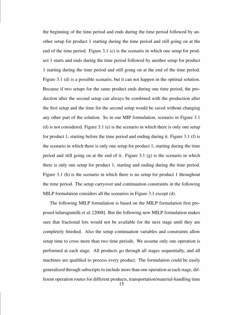
the beginning of the time period and ends during the time period followed by an-

other setup for product 1 starting during the time period and still going on at the

end of the time period. Figure 3.1 (c) is the scenario in which one setup for prod-

uct 1 starts and ends during the time period followed by another setup for product

1 starting during the time period and still going on at the end of the time period.

Figure 3.1 (d) is a possible scenario, but it can not happen in the optimal solution.

Because if two setups for the same product ends during one time period, the pro-

duction after the second setup can always be combined with the production after

the first setup and the time for the second setup would be saved without changing

any other part of the solution. So in our MIP formulation, scenario in Figure 3.1

(d) is not considered. Figure 3.1 (e) is the scenario in which there is only one setup

for product 1, starting before the time period and ending during it. Figure 3.1 (f) is

the scenario in which there is only one setup for product 1, starting during the time

period and still going on at the end of it. Figure 3.1 (g) is the scenario in which

there is only one setup for product 1, starting and ending during the time period.

Figure 3.1 (h) is the scenario in which there is no setup for product 1 throughout

the time period. The setup carryover and continuation constraints in the following

MILP formulation considers all the scenarios in Figure 3.1 except (d).

The following MILP formulation is based on the MILP formulation first pro-

posed inJarugumilli et al. [2008]. But the following new MILP formulation makes

sure that fractional lots would not be available for the next stage until they are

completely finished. Also the setup continuation variables and constraints allow

setup time to cross more than two time periods. We assume only one operation is

performed at each stage. All products go through all stages sequentially, and all

machines are qualified to process every product. The formulation could be easily

generalized through subscripts to include more than one operation at each stage, dif-

ferent operation routes for different products, transportation/material-handling time15

(a) one setup for product 1 going on

thoughout the time period

(b) two setups for product 1 going on at

the beginning and end of the time period

(c) two setups for product 1 going on in the

middle and at the end of the time period

(d) two setups for product 1 going on at the

beginng and in the middle the time period

(e) only one setup for product 1 going on

at the beginning of the time period

(f) only one setup for product 1 going on

at the end of the time period

(g) only one setup for product 1 done in

the middle of the time period

(h) no setup for product 1 throughout the

time period

Figure 3.1: Setup Scenarios During One Time Period

between operations, product-machine qualification, and product substitution (sub-

stitute lower-speed chips with faster-speed chips) in the semiconductor back-end

process. We have already implemented the generalized model with all those exten-

sions, which is shown in Appendix A. In the generalized formulation, if bottleneck

stages are identified, only the bottleneck stages will be included in the model first so

that the problem size can be decreased. Estimated throughput times of those non-

bottleneck stages from historical data are used to model delays between bottleneck

stages.

Notation:

P: number of products, with index p

N: number of stages, with index n

M[n]: number of parallel machines at stage n

16

T : number of time periods, with index t

K: a big number

C: capacity of one machine per time period, which can also be machine and/or

time period dependant denoted by Cn,m,t

Bp,0: initial back order quantity (in lots) of product p

Ip,n,0: initial integral inventory (in lots) of product p after stage n

Xp,n,m,0: initial fractional production quantity (in lots) of product p on machine

m at stage n

bp: back order cost of product p per lot per time period

dp,t : demand quantity (in lots) of product p at the end of time period t

sp,n,m : set up time for product p on machine m at stage n

tp,n,m : lot processing time of product p on machine m at stage n

Continuous Decision Variables:

Xp,n,m,t : production quantity (in lots) for product p on machine m at stage n in

time period t

Xp,n,m,t : fractional(unfinished) production quantity (in lots) for product p on

machine m at stage n at the end of time period t

W 1p,n,m,t : time for the setup that ends in time period t for product p on machine

m at stage n in time period t

W 2p,n,m,t : time for the setup time that continues in time period t +1 for product

p on machine m at stage n in time period t

Lp,n,m,t : cumulative setup time for an unfinished setup in process at the end of

time period for product p on machine m at stage n

Integer Decision Variables:

Xp,n,m,t : integral production quantity (in lots) for product p finished on machine

m at stage n in time period t

⌈X⌉p,n,m,t : smallest integer that is equal to or larger than Xp, n, m, t17

Ip,n,t : integral inventory quantity (in lots) of product p at the end of time period

t after stage n

Bp,t : integral back order quantity (in lots) of the product p at the end of time

period t

Binary Decision Variables:

Yp,n,m,t : 1 if a setup for product p on machine m at stage n ends in period t; 0

otherwise

Zp,n,m,t : 1 if product p can be processed on machine m at stage n in time period

t +1 without a setup; 0 otherwise

Up,n,m,t : 1 if a setup for product p is going on at the end of the period t and will

continue at the beginning of period t +1 on machine m at stage n; 0 otherwise

[BPSS]

min ∑p,t

bpBp,t (3.1)

s.t. Ip,n,t−1 +∑m

Xp,n,m,t −∑m

Xp,n+1,m,t −∑m⌈X⌉p,n+1,m,t +∑

m⌈X⌉p,n+1,m,t−1

= Ip,n,t , ∀ p,n < N, t (3.2)

∑m

Xp,n,m,t +∑m⌈X⌉p,n,m,t −∑

m⌈X⌉p,n,m,t−1 ≤ Ip,n−1,t−1, ∀p,n ≥ 2, t (3.3)

Ip,Np,t−1 −Bp,t−1 +∑m

Xp,Np,m,t −dp,t = Ip,Np,t −Bp,t , ∀p, t (3.4)

Xp,n,m,t−1 +Xp,n,m,t = Xp,n,m,t + Xp,n,m,t , ∀p,n,m, t (3.5)

⌈X⌉p,n,m,t −1 < Xp,n,m,t ≤ ⌈X⌉p,n,m,t , ∀p,n,m, t (3.6)

∑p

tp,n,mXp,n,m,t +∑p(W 1

p,n,m,t +W 2p,n,m,t)≤C, ∀n,1 ≤ m ≤ M[n], t (3.7)

Xp,n,m,t ≤ K(Zp,n,m,t−1 +Yp,n,m,t), ∀p,n,m, t (3.8)

W 1p,n,m,t ≤CYp,n,m,t , ∀p,n,m, t (3.9)

18

W 2p,n,m,t ≤CUp,n,m,t , ∀p,n,m, t (3.10)

∑p

Zp,n,m,t +∑p

Up,n,m,t = 1, ∀n,1 ≤ m ≤ M[n], t (3.11)

Zp,n,m,t ≤ 1+Yp,n,m,t −Yq,n,m,t , ∀p = q,n,m, t (3.12)

Zp,n,m,t ≤ Yp,n,m,t +Zp,n,m,t−1, ∀p,n,m, t (3.13)

sp,n,mYp,n,m,t ≤ Lp,n,m,t−1 +W 1p,n,m,t , ∀p,n,m, t (3.14)

Lp,n,m,t ≤ sp,n,mUp,n,m,t , ∀p,n,m, t (3.15)

Lp,n,m,t −W 2p,n,m,t ≤ Lp,n,m,t−1, ∀p,n,m, t (3.16)

Lp,n,m,t −W 2p,n,m,t ≤ sp,n,m ∗ (1−Yq,n,m,t), ∀p,q,n,m, t (3.17)

Xp,n,m,t ≤ Zp,n,m,t , ∀p,n,m, t (3.18)

0 ≤ Xp,n,m,t < 1, ∀p,n,m, t (3.19)

Xp,n,m,t , Xp,n,m,t ,W 1p,n,m,t ,W

2p,n,m,t ,Lp,n,m,t ∈ R+, ∀p,n,m, t (3.20)

Xp,n,m,t ,⌈X⌉p,n,m,t , Ip,n,t ,Bp,t ∈ Z+,∀p,n,m, t (3.21)

Yp,n,m,t ,Zp,n,m,t ,Up,n,m,t ∈ B,∀p,n,m, t (3.22)

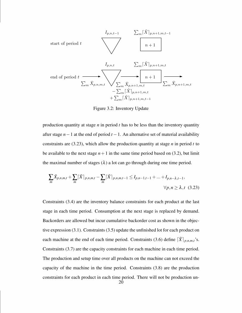
The objective in (3.1) is to minimize the total cumulative prioritized backorder

cost. Constraints (3.2) are the inventory balance constraints for each product at

each stage except the last in each time period. They indicate that the inventory

quantity at the end of current time period must equal to the previous inventory

plus production minus consumption at next operation. ∑m Xp,n+1,m,t is the total

number of lots finished at stage n+ 1 in period t, ∑m⌈X⌉p,n+1,m,t is the number

of unfinished lots on the machines at stage n+ 1 at the beginning of period t, and

∑m⌈X⌉p,n+1,m,t−1 is the number of lots still in process at stage n+ 1 at the end of

period t. ∑m Xp,n+1,m,t −∑m⌈X⌉p,n+1,m,t +∑m⌈X⌉p,n+1,m,t−1 is the number of lots

taken from the inventory Ip,n,t−1 at stage n+1 in time period t , as shown in Figure

3.2. Constraints (3.3) are the material availability constraints, which state that the

19

start of period t

Ip,n,t−1

∑m⌈X⌉p,n+1,m,t−1

end of period t

Ip,n,t

∑m⌈X⌉p,n+1,m,t

∑m

Xp,n,m,t

∑m

Xp,n+1,m,t

n + 1

n + 1∑

mXp,n+1,m,t

−∑

m⌈X⌉p,n+1,m,t

+∑

m⌈X⌉p,n+1,m,t−1

Figure 3.2: Inventory Update

production quantity at stage n in period t has to be less than the inventory quantity

after stage n−1 at the end of period t−1. An alternative set of material availability

constraints are (3.23), which allow the production quantity at stage n in period t to

be available to the next stage n+1 in the same time period based on (3.2), but limit

the maximal number of stages (λ ) a lot can go through during one time period.

∑m

Xp,n,m,t +∑m⌈X⌉p,n,m,t −∑

m⌈X⌉p,n,m,t−1 ≤ Ip,n−1,t−1 + ...+ Ip,n−λ ,t−1,

∀p,n ≥ λ , t (3.23)

Constraints (3.4) are the inventory balance constraints for each product at the last

stage in each time period. Consumption at the next stage is replaced by demand.

Backorders are allowed but incur cumulative backorder cost as shown in the objec-

tive expression (3.1). Constraints (3.5) update the unfinished lot for each product on

each machine at the end of each time period. Constraints (3.6) define ⌈X⌉p,n,m,t’s.

Constraints (3.7) are the capacity constraints for each machine in each time period.

The production and setup time over all products on the machine can not exceed the

capacity of the machine in the time period. Constraints (3.8) are the production

constraints for each product in each time period. There will not be production un-20

less a setup is carried over from last time period or finished in current time period.

Setup carryover is modeled by decision variables Zp,n,m,t’s. Zp,n,m,t = 1 means that

a setup for product p is carried over from time period t to t + 1 so that at the be-

ginning of time period t + 1 product p can be processed on machine m at stage n

without a setup. Constraints (3.9) constraint setup continuation decision variables

W 1p,n,m,t’s, saying that there is a positive setup time ending in this time period only

when a setup is finished in that time period. Constraints (3.10) define setup contin-

uation decision variables W 2p,n,m,t’s. There is a positive setup time continuing in the

next time period only when the setup is not finished at the end of the time period.

Constraints (3.11) indicate that at the end of any time period, a machine is either

being setup or producing for a product. Constraints (3.12) indicate that if there is

a setup finished for product q in the time period, the setup status for product p can

be carried over to the next time period only when there is also a setup finished for

product p. Constraints (3.13) indicate that the setup status can be carried over to the

next time period only when there is a setup finished in the time period or a setup car-

ryover from last time period. Constraints (3.14) link L1p,n,m,t with L2

p,n,m,t−1 through

t− 1 t t+ 1

W1p,n,m,t+1 = 0.5

W2p,n,m,t+1 = 0

Lp,n,m,t+1 = 1.8

Yp,n,m,t−1 = 1

Zp,n,m,t−1 = 1

Up,n,m,t−1 = 0

W1p,n,m,t = 0

W2p,n,m,t = 1

Lp,n,m,t = 1.3

Yp,n,m,t−1 = 0

Zp,n,m,t−1 = 0

Up,n,m,t−1 = 1

W1p,n,m,t−1 = 0

W2p,n,m,t−1 = 0.3

Lp,n,m,t−1 = 0.3

Yp,n,m,t−1 = 0

Zp,n,m,t−1 = 0

Up,n,m,t−1 = 1

Figure 3.3: Setup Continuation

W 1p,n,m,t . Constraints (3.15) say that L2

p,n,m,t’s can be positive only when there is a

setup continuing at the end of the time period based on the definition. Constraints21

(3.16) indicate the potential link between L2p,n,m,t and W 2

p,n,m,t +L2p,n,m,t−1 and con-

straints (3.17) limit L2p,n,m,t to W 2

p,n,m,t when there is a setup finished in time period t.

The relations among W 1p,n,m,t , W 2

p,n,m,t , and Lp,n,m,t as well as how they are updated

across time periods are shown in Figure 3.3 with a simple example. The example

shows a setup for product p on machine m at stage n across three time periods t−1,

t, and t +1. The setup starts at t −1+0.7, ends at t +1+0.5, and lasts for 1.8 time

periods. The values of W 1p,n,m, W 2

p,n,m, and Lp,n,m are shown in Figure 3.3 for each

time period. In real semiconductor manufacturing, setup can span several time pe-

riods but not shifts (1 shift = 12 hrs), which can be included in the model by adding

an additional set of constraints forcing Up,n,m,t’s during end-of-shift periods to be

zero. Constraints (3.18) make sure the scheduling process is non-preemptive. All

the remaining constraints (3.19), (3.20), (3.21), (3.22) are boundary, integral, and

binary constraints.

The above MILP formulation is an innovative way of modeling the flexible

flow shop scheduling problem. The optimal solution or a good upper bound of the

above MILP model is very important to the flexible flow shop scheduling research

because it can be used to evaluate the optimality of heuristic solutions. However, the

size and solution difficulty of the above MILP formulation increase quickly when

the problem size increases such as the number of products, number of machines,

demand, etc. Take a real semiconductor back-end facility for example, there are

about 25 products, 3 stages with 10,1,36 machines, and 168 2-hr time periods

(for 2 weeks). This gives us 25 × (10 + 1 + 36)× 168 = 197,400 of Xp,n,m,t’s,

Xp,n,m,t’s, Xp,n,m,t’s, ⌈X⌉p,n,m,t’s, W 1p,n,m,t’s, W 2

p,n,m,t’s, Lp,n,m,t’s, Yp,n,m,t’s, Zp,n,m,t’s,

Up,n,m,t’s each, which are 197,400×5 = 987,000 continuous variables, 197,400×

2 = 394,800 integer variables, 197,400×3 = 592,200 binary variables. There are

25× 3× 168+ 25× 168 = 16,800 more integer variables for Ip,n,t’s, and Bp,t’s.

Constraints (3.2) to (3.19) generates more than 11 million constraints. A C++ code22

using ILOG CPLEX11.2 concert technology is developed in a PC with windown

XP operating system and 2GB memory. The program runs out of memory before

generating the complete formulation for the above real facility example. Since the

problem is NP-hard, it could take a long time to solve some small size problems,

as shown in Section 5.1. As a result, for the daily scheduling in a real factory, A

deterministic scheduling system is presented in the following section, which not

only contains all additional important constraints in the factory but also runs in

reasonable time for online scheduling.

23

CHAPTER 4

DETERMINISTIC SCHEDULING SYSTEM (DSS)

The MILP formulation in Section 3 is very difficult to solve and thus can not be

implemented in the factory for daily production planning and scheduling purpose.

Besides, there are additional rules in the factory, e.g. preventive maintenance sched-

ule, sequence dependant setup, staff availability for setting up machines. In the

DSS, the following additional rules will be included:

• sequence dependent setup time: setup time depends on the previous prod-

uct and current product based on the similarity between them as well as the

operation being performed

• machine qualification/dedication: each machine will only be qualified to pro-

cess certain products

• machine preventive maintenance (PM) schedule: preventive maintenance for

each machine has to be done before the scheduled deadline

• machine engineering time (ET) schedule: engineering time schedule for each

machine have to be done during the exact scheduled time period

• resource availability related to setup or production activities: including staff

availability and tool set availability

• carrier capacities that limit the work-in-process inventories between certain

stages

It is difficult to model all those additional details and rules in a mathematical

scheduling model. To obtain a fairly good production schedule while still con-

sidering all the important rules in the factory, the DSS is proposed consisting of

a optimizing module followed by a scheduling module (Figure 4.1). The optimiz-

ing module, which is called optimizer, generates an optimal production plan from

a linear-programming (LP) formulation relaxed from the MILP formulation with

the production quantity at each stage for each product in each time period. Nei-

ther setups nor individual machines are modeled explicitly in the LP formulation.

Instead, they are modeled indirectly by decreasing machine capacity by a certain

percentage or counting number of qualified machines at a certain stage. Two dif-

ferent optimizers are used in the DSS: one is the LP relaxation, thus called the LP

optimizer, and the other is based on a backward capacity allocation logic similar to

a Material-Requirements-Planning (MRP) system, thus called the MRP optimizer.

Factory Data

Optimizer SchedulerProduction Plan

Detailed Production Schedule;Machine Utilization;

Missed Demand; etc.

Figure 4.1: Deterministic Scheduling System (DSS)

The scheduling module, which is called the scheduler, has a deterministic dis-

crete event system structure, and records events (setups, productions, PM’s, and

ET’s), statistics (queue length in front of each stage, machine utilization, through-

25

put time of each lot, etc.), status of resources (machines, staff), and material trans-

fer (lots moving from one stage to the next) in the factory. There are two important

scheduling rules in the scheduler, the dynamic lot prioritization (DLP) rule and the

dynamic machine prioritization (DMP) rule. The DLP rule is used to prioritize

lots in the queue when a machine becomes available, based on the product priority,

setup time needed, status of other machines in the same stage, staff availability, ma-

chine qualification, PM/ET schedules, and the production plan from the optimizer.

The DMP rule is used to choose a machine from a stage for a newly arrived lot,

based on similar information applied in the DLP rule. Both rules are dynamic, as

time changes the lot and machine priorities change too. Additional scheduling rules

are also developed to improve the production schedule for multiple secondary ob-

jectives, e.g. concurrent setup limits to limit the number of setups, work-in-process

(WIP) inventory limits to control the cycle time, and lot release control to avoid

over production.

4.1 Optimizer

Two optimizers are developed to provide a production plan with a production quan-

tity for each product at each stage during each time period as an input to the sched-

uler. The MRP optimizer takes each demand quantity with the due date and cal-

culates the latest production start time (LPST ) backward at each stage by counting

back the lead-time, as shown in Equation (4.1) and Equation (4.2).

LPSTp,t,Np = t −max{Dp,t × tp,Np

MP[Np], tp,Np}, for stage Np (4.1)

LPSTp,t,n = LPSTp,t,n+1 −max{Dp,t × tp,n

Mp[n], tp,n}, for stage n = Np −1 to 1 (4.2)

where,

Dp,t = demand quantity for product p in time period t,

LPSTp,t,n = latest production start time at stage n for the Dp,t lots for product p in

26

time period t,

tp,n = lot processing time for product p at stage n,

Mp[n] = number of machines qualified for product p at stage n.

For each demand quantity Dp,t for product p with the due date t, the calculation

process starts at the last stage Np. In order to satisfy the demand quantity Dp,t

at the end of time period t, the production should be started at stage Np no later

than time period LPSTp,t,Np given by Equation (4.1), since it would take at least

the amount of time given by max{Dp,t∗tp,NpMP[Np]

, tp,p} to finish the production at stage

Np. Then Equation (4.2) calculates the latest production start time period LPSTp,t,n

from stage Np −1 to stage 1 sequentially.

An alternative method to the above MRP optimizer is not to assign the same

LPST for all the Dp,t lots for product p in time period t. Instead, the Dp,t lots will

be allocated evenly in the max{Dp,t×tp,nMP[n]

, tp,n} time periods at stage n, each of which

will be assigned as the LPST for all the lots allocated in it. Thus in this plan, the

LPST ’s of some lots are larger than those in the MRP plan. However, the following

linear programming formulation could generate a better plan than the alternative

method within a reasonable time, so this alternative method is not included in the

computational experiment.

From the MRP optimizer, all the lots of the same product with the same due

date have the same LPST ’s at each stage. Machine capacity shared between dif-

ferent products is not considered. All qualified machines are assumed to be fully

available. The following LP optimizer will generate a more accurate LSPT for each

lot while considering machine capacity interaction between products. The mathe-

matical formulation for the LP optimizer is shown below. It is a simplified linear

relaxation of the MILP formulation in Section 3. This LP formulation does not

consider setup or individual machines. But it does consider qualification relations

between products and machines indirectly through available capacity for products27

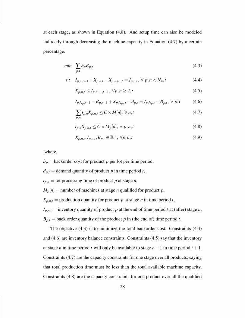
at each stage, as shown in Equation (4.8). And setup time can also be modeled

indirectly through decreasing the machine capacity in Equation (4.7) by a certain

percentage.

min ∑p,t

bpBp,t (4.3)

s.t. Ip,n,t−1 +Xp,n,t −Xp,n+1,t = Ip,o,t , ∀ p,n < Np, t (4.4)

Xp,n,t ≤ Ip,n−1,t−1, ∀p,n ≥ 2, t (4.5)

Ip,Np,t−1 −Bp,t−1 +Xp,Np, t −dp,t = Ip,Np,t −Bp,t , ∀ p, t (4.6)

∑p,m

tp,nXp,n,t ≤C×M[n], ∀ n, t (4.7)

tp,nXp,n,t ≤C×Mp[n], ∀ p,n, t (4.8)

Xp,n,t , Ip,n,t ,Bp,t ∈ R+, ∀p,n, t (4.9)

where,

bp = backorder cost for product p per lot per time period,

dp,t = demand quantity of product p in time period t,

tp,n = lot processing time of product p at stage n,

Mp[n] = number of machines at stage n qualified for product p,

Xp,n,t = production quantity for product p at stage n in time period t,

Ip,n,t = inventory quantity of product p at the end of time period t at (after) stage n,

Bp,t = back order quantity of the product p in (the end of) time period t.

The objective (4.3) is to minimize the total backorder cost. Constraints (4.4)

and (4.6) are inventory balance constraints. Constraints (4.5) say that the inventory

at stage n in time period t will only be available to stage n+1 in time period t +1.

Constraints (4.7) are the capacity constraints for one stage over all products, saying

that total production time must be less than the total available machine capacity.

Constraints (4.8) are the capacity constraints for one product over all the qualified

28

machines at one stage, saying that the production time for one product must be less

than the available qualified machine capacity.

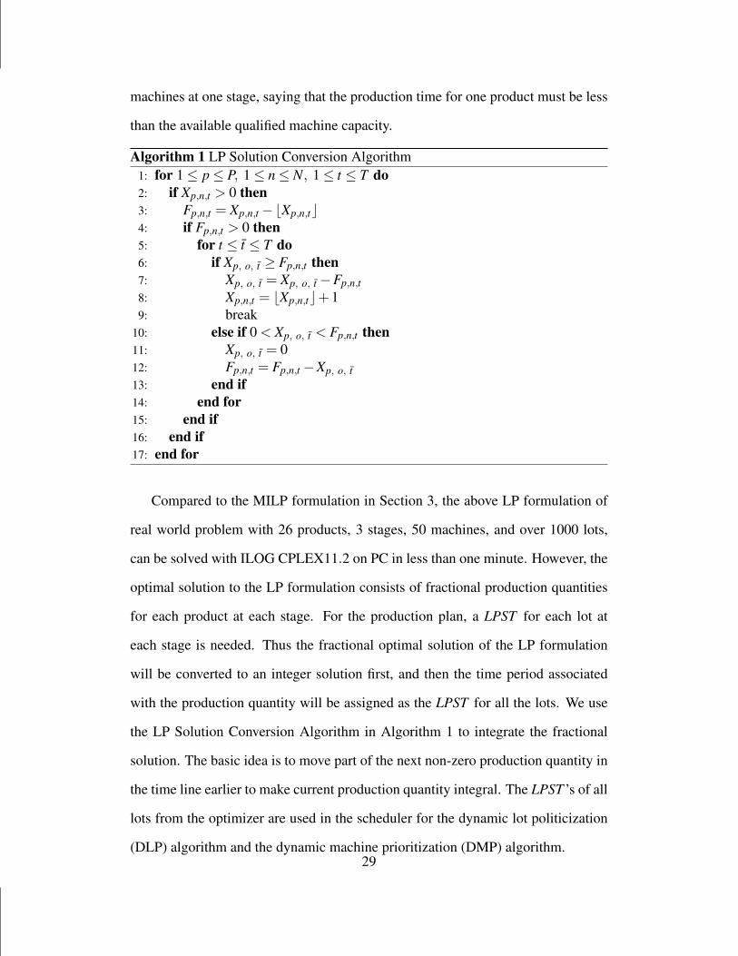
Algorithm 1 LP Solution Conversion Algorithm1: for 1 ≤ p ≤ P, 1 ≤ n ≤ N, 1 ≤ t ≤ T do2: if Xp,n,t > 0 then3: Fp,n,t = Xp,n,t −⌊Xp,n,t⌋4: if Fp,n,t > 0 then5: for t ≤ t ≤ T do6: if Xp, o, t ≥ Fp,n,t then7: Xp, o, t = Xp, o, t −Fp,n,t8: Xp,n,t = ⌊Xp,n,t⌋+19: break

10: else if 0 < Xp, o, t < Fp,n,t then11: Xp, o, t = 012: Fp,n,t = Fp,n,t −Xp, o, t13: end if14: end for15: end if16: end if17: end for

Compared to the MILP formulation in Section 3, the above LP formulation of

real world problem with 26 products, 3 stages, 50 machines, and over 1000 lots,

can be solved with ILOG CPLEX11.2 on PC in less than one minute. However, the

optimal solution to the LP formulation consists of fractional production quantities

for each product at each stage. For the production plan, a LPST for each lot at

each stage is needed. Thus the fractional optimal solution of the LP formulation

will be converted to an integer solution first, and then the time period associated

with the production quantity will be assigned as the LPST for all the lots. We use

the LP Solution Conversion Algorithm in Algorithm 1 to integrate the fractional

solution. The basic idea is to move part of the next non-zero production quantity in

the time line earlier to make current production quantity integral. The LPST ’s of all

lots from the optimizer are used in the scheduler for the dynamic lot politicization

(DLP) algorithm and the dynamic machine prioritization (DMP) algorithm.29

4.2 Scheduler

Initialization

System State

Event List

Advance Clock to

Time of Next Event

Update State

Schedule Event

Remove Event from

Event List

Stop

No

Yes Summary

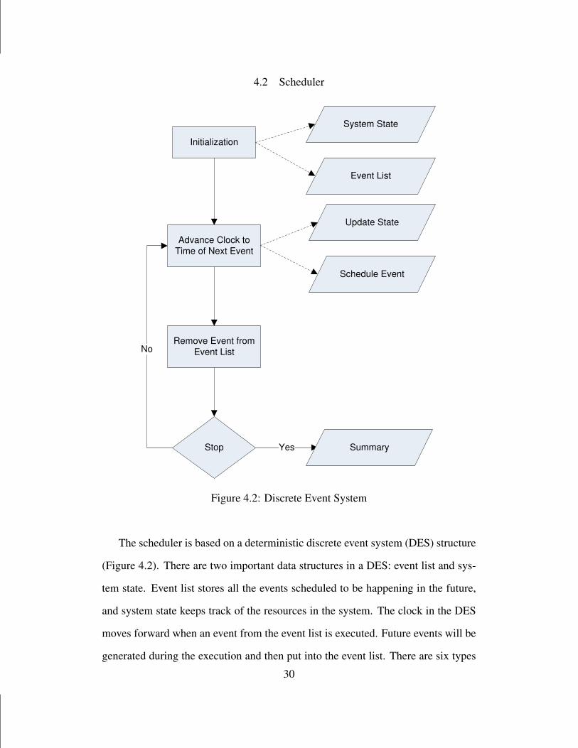
Figure 4.2: Discrete Event System

The scheduler is based on a deterministic discrete event system (DES) structure

(Figure 4.2). There are two important data structures in a DES: event list and sys-

tem state. Event list stores all the events scheduled to be happening in the future,

and system state keeps track of the resources in the system. The clock in the DES

moves forward when an event from the event list is executed. Future events will be

generated during the execution and then put into the event list. There are six types

30

of events in the scheduler: lot arrival to a stage, lot departure from a machine, end

of a setup, end of a PM, end of an ET, and start of a time period. The following

information is collected during the scheduling process: machine utilization, cycle

time of each lot, queue length in front of each stage, etc. When a lot arrival event

happens, the dynamic machine prioritization (DMP) rule in Algorithm 2 will be

used to choose a machine from the stage to process this lot. The DMP rule priori-

tizes the machines at a stage based on the setup time and checks the eligibility of the

setup/production based on the availability of setup staff (if setup needed), related

customized factory rules (PM/ET schedules) and scheduling control rules (machine

setup limit to be discussed later). If no machine is available or eligible, the lot will

be waiting in the queue. It should be noted that before every lot processed, the

scheduler will check the eligibility of the production and/or setup according to the

following three criteria: (1) whether there is an available staff to perform the setup

(if a setup is needed), (2) whether the number of machines setup for the product

at this stage is less than the machine setup limit for the product at the stage, and

(3) whether the production and/or setup will violate any PM or ET schedule. The

machine setup limit is an adjustable parameter in the scheduler, which is used to

control the number of setups in the scheduling process. When a lot departure event

happens, a machine becomes idle and the dynamic lot prioritization (DLP) rule in

Algorithm 3 will be used to choose a lot from the queue. The DLP prioritizes the

lots in a queue based on their LPST ’s and the setup time, and at the same time

checks the eligibility of the setup/production. When an end of setup/PM/ET event

happens, a machine as well as a setup staff become available, and thus all the idle

machines in the system will be scheduled using the DLP rule. In the second row of

the DLP rule in Algorithm 3, all the eligible and qualified lots are ranked based on

their priorities and LPST ’s. The ranking criteria are: (1) late lots are ranked based

on their priorities, the higher the priority, the higher the rank; (2) all late lots are31

ranked higher than all early lots; (3) early lots are ranked based on their LPST ’s,

the earlier the LPST , the higher the rank. A lot is defined as late when its LPST

is smaller than or equal to the current clock time in the system, and early when its

LPST is larger than the current clock time in the system. Since the LPST of a lot is

an important factor during the ranking process, the result from the DLP rule could

be different when the clock time proceeds. As a result, at the beginning of each

time period, all the idle machines in the system will be scheduled using the DLP

rule too.

The main output of the DSS is a detailed schedule for each machine over the

planning horizon with the exact start and finish time of each lot processing, setup,

PM, or ET operation. Another output is a summary including the total execution

time of the scheduling system, average utilization for each machine, average uti-

lization for each staff, average cycle time for each product, total number of setups

for each stage, average queue length for each stage, and shortages for each product.

4.3 Parameters

There are several adjustable parameters for the deterministic scheduling system,

which could be used to optimize the DSS under different objectives or scenarios.

• Optimizer: LP optimizer or MRP optimizer.

• Lot Release Control: whether release all lots into the DSS at the beginning

of the planning horizon or only release lots with LPST ’s in a week at the

beginning of the week, assuming weekly demands.

• Setup Control Level αp: a multiplier used to set the number of machines al-

lowed to be setup concurrently for product p at stage n, Sp,n =αp×Dp×tnp

∑p Dp×tp,n×

M[n]. So if there are already Sp,n machines setup for product p at stage n, no

32

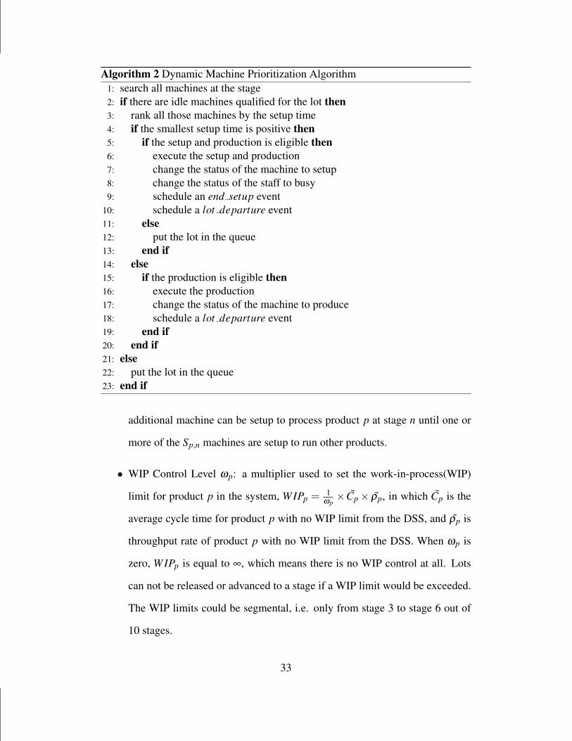
Algorithm 2 Dynamic Machine Prioritization Algorithm1: search all machines at the stage2: if there are idle machines qualified for the lot then3: rank all those machines by the setup time4: if the smallest setup time is positive then5: if the setup and production is eligible then6: execute the setup and production7: change the status of the machine to setup8: change the status of the staff to busy9: schedule an end setup event

10: schedule a lot departure event11: else12: put the lot in the queue13: end if14: else15: if the production is eligible then16: execute the production17: change the status of the machine to produce18: schedule a lot departure event19: end if20: end if21: else22: put the lot in the queue23: end if

additional machine can be setup to process product p at stage n until one or

more of the Sp,n machines are setup to run other products.

• WIP Control Level ωp: a multiplier used to set the work-in-process(WIP)

limit for product p in the system, WIPp =1

ωp× Cp × ρp, in which Cp is the

average cycle time for product p with no WIP limit from the DSS, and ρp is

throughput rate of product p with no WIP limit from the DSS. When ωp is

zero, WIPp is equal to ∞, which means there is no WIP control at all. Lots

can not be released or advanced to a stage if a WIP limit would be exceeded.

The WIP limits could be segmental, i.e. only from stage 3 to stage 6 out of

10 stages.

33

Algorithm 3 Dynamic Lot Prioritization Algorithm1: search the queue for qualified and eligible lots2: rank all those lots based on their priorities and LPST ’s3: if there is no qualified and eligible lot then4: if there is a qualified lot that can not be scheduled only because of conflicting

a scheduled PM/ET then5: execute the PM/ET6: change the status of the machine from idle to PM/ET7: schedule a PM/ET end event8: else9: leave the machine idle

10: end if11: else if the lot with the highest rank is an early lot then12: if there is a qualified late lot that can not be scheduled only because of con-

flicting a scheduled PM then13: execute the PM14: change the status of the machine from idle to PM15: schedule a PM end event16: else17: execute the production18: change the status of the machine from idle to producing19: schedule a lot depart event20: end if21: else if the lot with the highest rank is a late lot then22: execute the production23: change the status of the machine from idle to producing24: schedule a lot depart event25: end if

34

CHAPTER 5

EXPERIMENT RESULTS

This section discusses the solvable size of the proposed BPSS formulation and the

performance of the DSS through randomly generated small size and real size prob-

lem instances. The BPSS formulation was implemented in C++ and solved using

CPLEX11.2 concert technology, compiled with Microsoft Visual C++. The DSS

was implemented in C++, compiled with Microsoft Visual C++. Both programs

were run on a PC with a Intel Xeon Dual Core 2.00 GHz, 2.00 GHz processor with

2 GB of RAM.

5.1 General Evaluation

Table 5.1: Toy Data Size

Number of Products P 2,3,4

Number of Stages S 2,3

Number of Weeks 2

Number of Periods in Each Week 5

Setup Time 0.5

Weekly Demand U(0,5)

Number of machines at Each Stage U(1,5)

Lot Processing Time U(0.5,1.5)

Table 5.2: DSS Parameter Values

Optimizer LP,MRP

Release Control Y,N

Setup Control Level α 1.0 ∼ 5.0 at step of 0.5

WIP Control Level ω 0, 14 ,

12 ,1,2

Twenty data sets are randomly generated according to each combination of fac-

tors for the small problems shown in Table 5.1, and then solved with both the BPSS

and the DSS. For those small problems, there is no initial backorder for any product;

only one operation is performed at each stage; all products follow the same route

from the first stage to the last stage; all machines are qualified for all products;

there is no initial WIP inventory in the system (start with an empty system); there is

no PM/ET schedule; the product index represents the product priority, lower index

meaning higher priority; the weight for the backorder of product p is defined as

bp = P− p+1, in which P is the total number of products; every machine needs a

setup for any product at the beginning, and the setup time is sequence independent.

Problem cases are denoted as PxSy for x products and y stages. Table 5.2 shows all

the parameter values used in the DSS, and the DSS solutions are chosen as the best

among all the parameter value combinations. The BPSS solutions were obtained

with CPLEX11.2 with an optimality gap of 0.01, no time limit for P2 problems,

and within 1 hour for P3 and P4 problems.

The summary of the BPSS and DSS solutions for small problems are shown in

Figure 5.1, with Box-and-Whiskers plots of the solutions at each method (BPSS/DSS)

and problem size (Product/Stage) combination in Figure 5.1a, and quartiles in Fig-

ure 5.1b. There are some P4S2 and P4S3 problems that BPSS could not find any

feasible solution or only obtain very large feasible solutions within the 1 hour time

limit. For those problems, the BPSS solutions are set to be 250 so that all solutions

can fit in one figure with a reasonable scale. We observe from Figure 5.1 that for

P2 and P3 problems the mean of BPSS solutions are slightly better than that of

DSS solutions under the objective of minimizing prioritized backorder cost. How-

ever, for P4 problems the mean of BPSS solutions are worse than that of the DSS

solutions. We did a matched pairs analysis of the BPSS solutions and DSS solu-

tions of small problems grouped according to product and stage combination, as

shown in Table 5.3. Matched pair analysis results in Table 5.3 show that the mean

of DSS solution is 11.35 smaller than that of the BPSS solutions and the difference36

is significant. Across groups results shows the mean difference (DSS mean - BPSS

mean) and mean mean (DSS mean + BPSS mean2 ) for each group (product stage

combination). Test across groups shows that the mean difference and mean mean

between groups are significantly different, which verifies that the mean difference

changes (decreases in magnitude) when problem size increases. As the problem

size increases, the performance of DSS becomes better than the BPSS. It should be

noted that in some cases, i.e. the 4th and 5th replicates of P2S3, the DSS solutions

are even better than the corresponding optimal BPSS solutions. The reason is that

the material is assumed to be moved at the end of every time period in BPSS while

the material movement is continuous in the DSS (a lot is available to the next stage

right after it is finished at current stage). We call this phenomenon the impact of

discretization.

The solution times for both the BPSS and the DSS are summarized in Table 5.4

with median and standard deviation for each product and stage combination. It can

be seen that the DSS has much smaller standard deviations compared to the BPSS

across all problem sizes, and increases much slower as the problem size increases.

5.2 Offline Optimization of the DSS Parameters with Single Objective

Experimental design is used to evaluate important factors affecting the DSS perfor-

mance and their interactions with a single objective of minimizing the total priori-

tized backorder cost. Those factors and their possible values to be evaluated in the

experiment are listed in Table 5.5. Different numbers of products represent different

levels of product mix. Three weekly demand distributions represent three demand

scenarios of interest: low demand level with small deviation, low demand level

with large deviation, and high demand level with small deviation. The machine uti-

lization level θ is used to determine the number of machines at each stage n using

M[n] = ⌈∑p Dp × tp,n/(C × θn)⌉. In the experiment, all machines are assumed to

37

0

50

100

150

200

250

Solu

tion

P2S

2_B

PS

S

P2S

2_D

SS

P2S

3_B

PS

S

P2S

3_D

SS

P3S

2_B

PS

S

P3S

2_D

SS

P3S

3_B

PS

S

P3S

3_D

SS

P4S

2_B

PS

S

P4S

2_D

SS

P4S

3_B

PS

S

P4S

3_D

SS

Data & Method

(a) Box-and-Whiskers Plots of Backorder Costs

P2S2_BPSS

P2S2_DSS

P2S3_BPSS

P2S3_DSS

P3S2_BPSS

P3S2_DSS

P3S3_BPSS

P3S3_DSS

P4S2_BPSS

P4S2_DSS

P4S3_BPSS

P4S3_DSS

Level

0

0

0

0

0

0

0

1

0

0

0

5

Minimum

0

0

0

0

0

0

3.4

6.1

0.1

0.1

13.4

18.7

10%

0

0

3

3

0.25

0

10.75

17

4.25

5

57

43.25

25%

1

1

9.5

10

4

5

32.5

37

52.5

35.5

95

64.5

Median

6

9

20

23.25

45.75

45.75

62.5

58.5

121.25

75

226

103

75%

22.3

25.4

34.6

35.3

74.7

77.7

83

87.8

241.5

130.3

250

214.5

90%

26

26

43

42

92

92

95

113

250

138

250

223

Maximum

(b) Quantiles of Backorder Costs

Figure 5.1: Solution Value Summary for Small Problem Instances

38

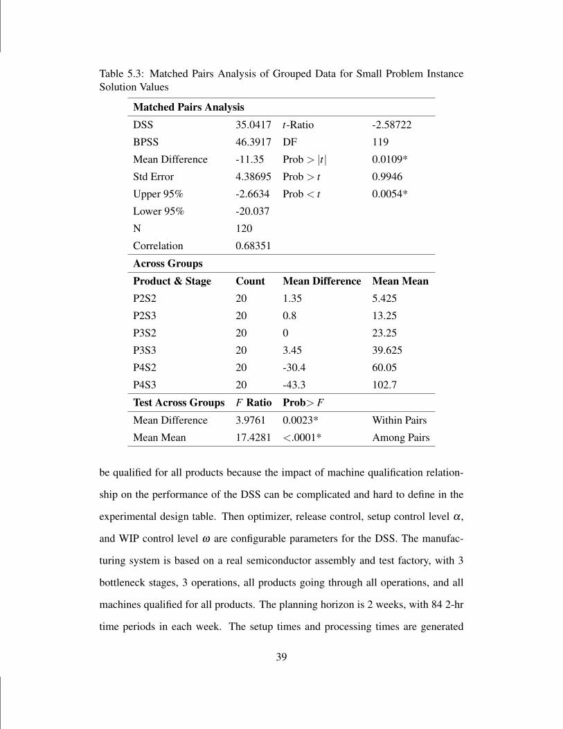
Table 5.3: Matched Pairs Analysis of Grouped Data for Small Problem InstanceSolution Values

Matched Pairs AnalysisDSS 35.0417 t-Ratio -2.58722

BPSS 46.3917 DF 119

Mean Difference -11.35 Prob > |t| 0.0109*

Std Error 4.38695 Prob > t 0.9946

Upper 95% -2.6634 Prob < t 0.0054*

Lower 95% -20.037

N 120

Correlation 0.68351

Across GroupsProduct & Stage Count Mean Difference Mean MeanP2S2 20 1.35 5.425

P2S3 20 0.8 13.25

P3S2 20 0 23.25

P3S3 20 3.45 39.625

P4S2 20 -30.4 60.05

P4S3 20 -43.3 102.7

Test Across Groups F Ratio Prob> F

Mean Difference 3.9761 0.0023* Within Pairs

Mean Mean 17.4281 <.0001* Among Pairs

be qualified for all products because the impact of machine qualification relation-

ship on the performance of the DSS can be complicated and hard to define in the

experimental design table. Then optimizer, release control, setup control level α ,

and WIP control level ω are configurable parameters for the DSS. The manufac-

turing system is based on a real semiconductor assembly and test factory, with 3

bottleneck stages, 3 operations, all products going through all operations, and all

machines qualified for all products. The planning horizon is 2 weeks, with 84 2-hr

time periods in each week. The setup times and processing times are generated

39

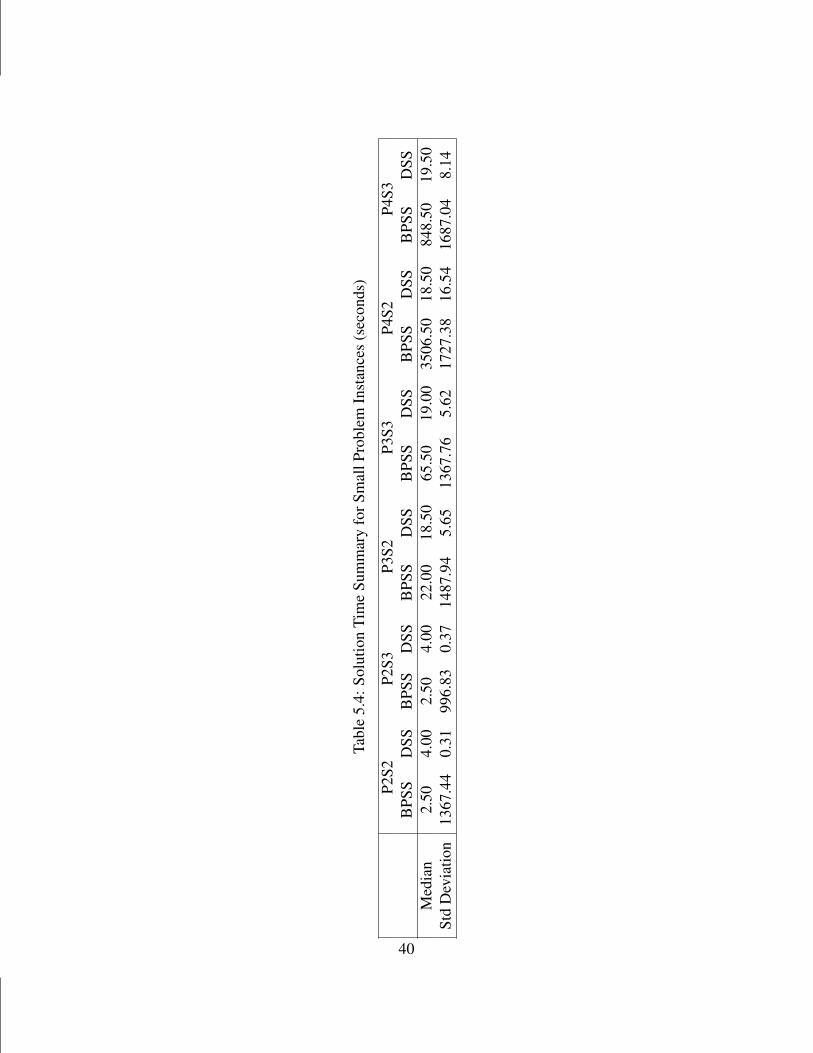
Tabl

e5.

4:So

lutio

nTi

me

Sum

mar

yfo

rSm

allP

robl

emIn

stan

ces

(sec

onds

)

P2S2

P2S3

P3S2

P3S3

P4S2

P4S3

BPS

SD

SSB

PSS

DSS

BPS

SD

SSB

PSS

DSS

BPS

SD

SSB

PSS

DSS

Med

ian

2.50

4.00

2.50

4.00

22.0

018

.50

65.5

019

.00

3506

.50

18.5

084

8.50

19.5

0St

dD

evia

tion

1367

.44

0.31

996.

830.

3714

87.9

45.

6513

67.7

65.

6217

27.3

816

.54

1687

.04

8.14

40

Number of Products 10,25,50

Weekly Demand U(40,60),U(10,90),U(80,120)

Machine Utilization θ 60%,90%

Optimizer LP,MRP

Release Control Y,N

Setup Control Level α 1.0 ∼ 5.0 at step of 0.5

WIP Control Level ω 0, 14 ,

12 ,1,2

Table 5.5: Independent Variables in the Experiment Design (Single Objective)

according to Table 5.1.

An experiment is designed with the DOE customer design function in JMP8 to

test all the main effects as shown in Table 5.5 and their two-factor interactions. The

experiment requires 540 runs (a 16 fractional design) with different combinations

of the factor values, and 10 replicates were used. The Analysis of Variance and

Effect Test results are shown in Table 5.6. RSquare of 0.71 means 71% of the vari-

ation in the response around the mean can be attributed to the terms in the model

rather than to random error. All the main effects and the two-factor interactions are

highly significant with P-value’s less than 0.0001. Based on the fitted model, the

Prediction Profiler in JMP8 recommends best configurations of the scheduler (Op-

timizer, Release Control, Setup Control Level, Control Level) which minimize the

response variable under different scenarios (Number of Product, Weekly Demand,

Machine Utilization), as shown in Table 5.7. The fitted model can also be used to

recommend the configuration of the scheduler that minimizes the maximal or mean

prioritized backorder cost over all scenarios, which are {LP, No Release Control,

α = 0.5, ω = 14} and {MRP, Release Control, α = 4, ω = 1

2} respectively.

Note that the LP model outperforms the MRP approach for large problems.

Likewise, release control is best in most cases and always best with a large number

of products (50). The optimal setup control parameter varies but always exceeds the

41

minimum feasible value of 1. In many cases values of 3.5 to 5 are best indicating

that available capacity should be utilized rather than focusing on minimizing setups.

In all but one case, the higher shop utilization level (90%) preferred as high or

higher setup control level than the case of 60% utilization. While this may seem

to waste time in extra setups, the exhaustive policy and due dates served to ensure

that capacity was not wasted in setups but the higher setup level allowed the system

to avoid wasting valuable capacity in the dynamic instances where certain products

accumulated at stages with others not being available for processing. The best

choice of WIP control was somewhat correlated with the mean demand level. At

the higher level of 100 lots per product per period the best WIP control level was 1

or higher in 5 of 6 cases. With a mean demand of 50 lots per period per product,

regardless of the number of products and size of the facility, a WIP control level of

12 was best in 9 of 12 cases. The three cases with higher WIP control, meaning more

restricted WIP levels, occurred with higher levels of demand variability (Uniformly

distributed between 10 and 90 instead of 40 to 60).

5.3 Offline Optimization of the DSS Parameters with Multiple Objectives

In this section, experimental design is used to evaluate important factors affecting

the DSS performance under multiple objectives. In this experiment, there are 3

stages and 4 operations. 2 operations are performed at the 3 stage. No setup is

needed at the second stage. A minor setup is needed between the 2 operations at

stage 3 for the same product. The planning period is 2 weeks and divided in to 168

2-hr time periods. The parameters and levels tested in the experiment are listed in

Table 5.8. Data sets are randomly generated and the control parameters of DSS are

set according to the values in the table. Exponential distribution is used to generate

weekly demand. Product-machine qualification is considered in this experiment.

The number of qualified machines for product p at stage n, NQp,n, is calculated

42

Table 5.6: Design of Experiment (Single Objective) Statistical Summary

Summary of FitRSquare 0.712727RSquare Adj 0.704292Root Mean Square Error 50783.52Mean of Response 28989.14Observations 5400Analysis of VarianceSource DF Sum of Squares Mean Square F Ratio Prob > FModel 154 3.36E +13 2.18E +11 84.4992 0.0000Error 5245 1.35E +13 2.58E +09C. Total 5399 4.71E +13Effect TestsSource N DF Sum of Squares F Ratio Prob > FNumber of Product (P) 2 2 4.17E+12 809.3092 <.0001Weekly Demand (D) 2 2 1.12E+12 216.7478 <.0001Machine Utilization (M) 1 1 2.80E+12 1084.732 <.0001Optimizer (O) 1 1 2.60E+12 1007.006 <.0001Release Control (R) 1 1 2.80E+12 1084.035 <.0001Setup Control (S) 8 8 3.30E+11 15.9711 <.0001WIP Control (W) 4 4 2.33E+11 22.5614 <.0001P×D 4 4 8.28E+11 80.2933 <.0001P×M 2 2 2.34E+12 454.5693 <.0001P×O 2 2 2.06E+12 400.0243 <.0001P×R 2 2 2.47E+12 478.756 <.0001P×O 16 16 4.20E+11 10.1707 <.0001P×W 8 8 2.69E+11 13.0305 <.0001D×M 2 2 4.44E+11 86.0589 <.0001D×O 2 2 8.37E+11 162.2237 <.0001D×R 2 2 5.54E+11 107.4433 <.0001D×O 16 16 4.75E+11 11.5161 <.0001D×W 8 8 4.06E+11 19.7001 <.0001M×O 1 1 1.30E+12 502.9219 <.0001M×R 1 1 1.67E+12 649.2165 <.0001M×O 8 8 3.20E+11 15.5078 <.0001M×W 4 4 1.43E+11 13.8729 <.0001O×R 1 1 2.59E+12 1004.306 <.0001O×O 8 8 9.62E+10 4.6613 <.0001O×W 4 4 1.34E+11 12.9555 <.0001R×O 8 8 1.19E+11 5.7581 <.0001R×W 4 4 2.31E+11 22.3957 <.0001O×W 32 32 1.14E+12 13.8229 <.0001

43

Table 5.7: Recommended Configuration Under Each Scenario (Single Objective)

Num. of Weekly Machine Optimizer Release Setup WIP

Product Demand Utilization Control Control Control

10 U(40,60) 60% MRP Y 4 1/2

10 U(40,60) 90% MRP Y 3.5 1/2

10 U(10,90) 60% LP N 1.5 0

10 U(10,90) 90% MRP Y 5 2

10 U(80,120) 60% LP N 1.5 1

10 U(80,120) 90% LP Y 5 2

25 U(40,60) 60% MRP Y 4 1/2

25 U(40,60) 90% LP Y 4 1/2

25 U(10,90) 60% MRP Y 4 1/2

25 U(10,90) 90% LP Y 4 1/2

25 U(80,120) 60% LP N 1.5 1

25 U(80,120) 90% LP Y 5 2

50 U(40,60) 60% LP Y 3.5 1/2

50 U(40,60) 90% LP Y 3.5 1/2

50 U(10,90) 60% LP Y 5 2

50 U(10,90) 90% LP Y 5 2

50 U(80,120) 60% LP Y 2 1/4

50 U(80,120) 90% LP Y 3 1

using Equation (5.1) as ϕp times the minimal number of machines needed, which

is the total demand, Dp,n, times processing time, tp,n, divided by single machine

capacity, 168.

NQp,n = ϕp ×Dp × tp,n/168 (5.1)

The load share for product p on each qualified machine at stage n, LSp,n, is calcu-

lated as LSp,n = Dp × tp,n/NQp,n. NQp,n load shares of product p are assign for

machines at stage n with most available capacity iteratively and then the available

capacity of the assigned machine is updated (minus the load share) after each itera-44

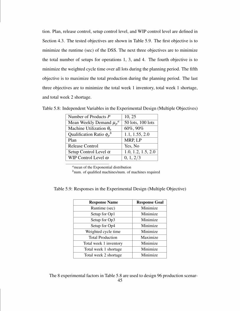
tion. Plan, release control, setup control level, and WIP control level are defined in

Section 4.3. The tested objectives are shown in Table 5.9. The first objective is to

minimize the runtime (sec) of the DSS. The next three objectives are to minimize

the total number of setups for operations 1, 3, and 4. The fourth objective is to

minimize the weighted cycle time over all lots during the planning period. The fifth

objective is to maximize the total production during the planning period. The last

three objectives are to minimize the total week 1 inventory, total week 1 shortage,

and total week 2 shortage.

Table 5.8: Independent Variables in the Experimental Design (Multiple Objectives)

Number of Products P 10, 25Mean Weekly Demand µp

a 50 lots, 100 lotsMachine Utilization θn 60%, 90%Qualification Ratio ϕp

b 1.1, 1.55, 2.0Plan MRP, LPRelease Control Yes, NoSetup Control Level α 1.0, 1.2, 1.5, 2.0WIP Control Level ω 0, 1, 2/3

amean of the Exponential distributionbnum. of qualified machines/num. of machines required

Table 5.9: Responses in the Experimental Design (Multiple Objective)

Response Name Response GoalRuntime (sec) MinimizeSetup for Op1 MinimizeSetup for Op3 MinimizeSetup for Op4 Minimize

Weighted cycle time MinimizeTotal Production Maximize

Total week 1 inventory MinimizeTotal week 1 shortage MinimizeTotal week 2 shortage Minimize

The 8 experimental factors in Table 5.8 are used to design 96 production scenar-45

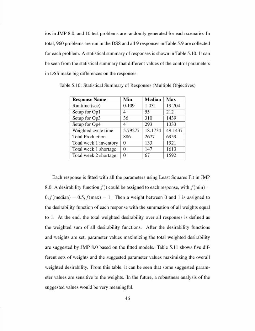
ios in JMP 8.0, and 10 test problems are randomly generated for each scenario. In

total, 960 problems are run in the DSS and all 9 responses in Table 5.9 are collected

for each problem. A statistical summary of responses is shown in Table 5.10. It can

be seen from the statistical summary that different values of the control parameters

in DSS make big differences on the responses.

Table 5.10: Statistical Summary of Responses (Multiple Objectives)

Response Name Min Median MaxRuntime (sec) 0.109 1.031 19.704Setup for Op1 4 55 212Setup for Op3 36 310 1439Setup for Op4 41 293 1333Weighted cycle time 5.79277 18.1734 49.1437Total Production 886 2677 6959Total week 1 inventory 0 133 1921Total week 1 shortage 0 147 1613Total week 2 shortage 0 67 1592

Each response is fitted with all the parameters using Least Squares Fit in JMP

8.0. A desirability function f () could be assigned to each response, with f (min) =

0, f (median) = 0.5, f (max) = 1. Then a weight between 0 and 1 is assigned to

the desirability function of each response with the summation of all weights equal

to 1. At the end, the total weighted desirability over all responses is defined as

the weighted sum of all desirability functions. After the desirability functions

and weights are set, parameter values maximizing the total weighted desirability

are suggested by JMP 8.0 based on the fitted models. Table 5.11 shows five dif-

ferent sets of weights and the suggested parameter values maximizing the overall

weighted desirability. From this table, it can be seen that some suggested param-

eter values are sensitive to the weights. In the future, a robustness analysis of the

suggested values would be very meaningful.

46

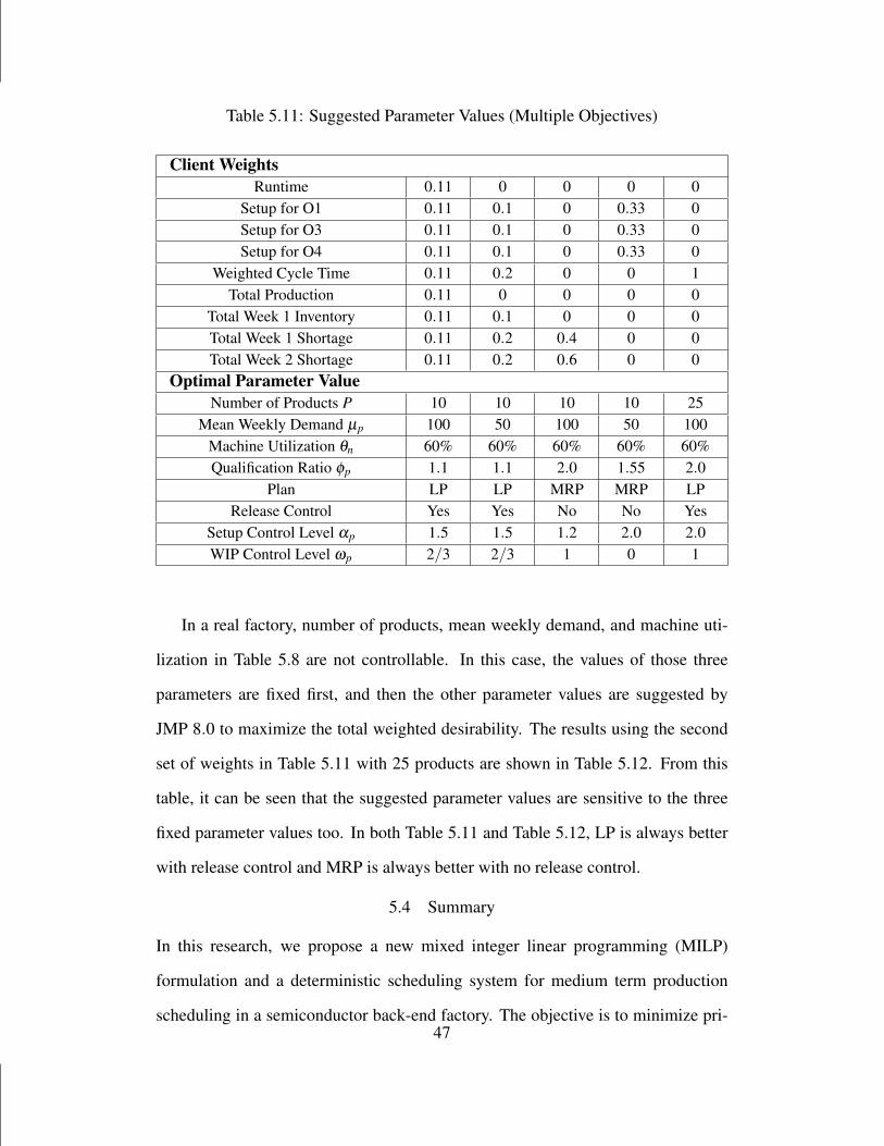
Table 5.11: Suggested Parameter Values (Multiple Objectives)

Client WeightsRuntime 0.11 0 0 0 0

Setup for O1 0.11 0.1 0 0.33 0Setup for O3 0.11 0.1 0 0.33 0Setup for O4 0.11 0.1 0 0.33 0

Weighted Cycle Time 0.11 0.2 0 0 1Total Production 0.11 0 0 0 0

Total Week 1 Inventory 0.11 0.1 0 0 0Total Week 1 Shortage 0.11 0.2 0.4 0 0Total Week 2 Shortage 0.11 0.2 0.6 0 0

Optimal Parameter ValueNumber of Products P 10 10 10 10 25

Mean Weekly Demand µp 100 50 100 50 100Machine Utilization θn 60% 60% 60% 60% 60%Qualification Ratio ϕp 1.1 1.1 2.0 1.55 2.0

Plan LP LP MRP MRP LPRelease Control Yes Yes No No Yes

Setup Control Level αp 1.5 1.5 1.2 2.0 2.0WIP Control Level ωp 2/3 2/3 1 0 1

In a real factory, number of products, mean weekly demand, and machine uti-

lization in Table 5.8 are not controllable. In this case, the values of those three

parameters are fixed first, and then the other parameter values are suggested by

JMP 8.0 to maximize the total weighted desirability. The results using the second

set of weights in Table 5.11 with 25 products are shown in Table 5.12. From this

table, it can be seen that the suggested parameter values are sensitive to the three

fixed parameter values too. In both Table 5.11 and Table 5.12, LP is always better

with release control and MRP is always better with no release control.

5.4 Summary

In this research, we propose a new mixed integer linear programming (MILP)

formulation and a deterministic scheduling system for medium term production

scheduling in a semiconductor back-end factory. The objective is to minimize pri-47

Table 5.12: Suggested Parameter Values with Three Fixed Parameters (MultipleObjectives)

Client WeightsRuntime 0 0 0 0

Setup for O1 0.1 0.1 0.1 0.1Setup for O3 0.1 0.1 0.1 0.1Setup for O4 0.1 0.1 0.1 0.1

Weighted Cycle Time 0.2 0.2 0.2 0.2Total Production 0 0 0 0

Total Week 1 Inventory 0.1 0.1 0.1 0.1Total Week 1 Shortage 0.2 0.2 0.2 0.2Total Week 2 Shortage 0.2 0.2 0.2 0.2

Fixed ParameterNumber of Products P 25 25 25 25

Mean Weekly Demand µp 50 50 100 100Machine Utilization θn 60% 90% 60% 90%

Optimal Controllable ParameterQualification Ratio ϕp 1.1 2.0 2.0 2.0

Plan LP MRP LP LPRelease Control Yes No Yes Yes

Setup Control Level αp 1.2 1.5 2.0 1.0WIP Control Level ωp 1 2/3 0 0

oritized tardiness with a model of relatively high fidelity to the actual factory. The

MILP formulation and the DSS are compared by solving randomly generated small

problem instances. The solution time of the MILP formulation can be long even for

a small problem, and the optimal solution to the MILP formulation can be worse

than the best DSS solution due to the impact of discretization. On the other hand,

the DSS solution time is relatively small and consistent, and by adjusting the pa-

rameter values the best DSS solution quality is satisfactory (50% of the time equal

to or better than the MILP optimal solution). The behavior of the DSS and the best

configurations under different scenarios are evaluated through experimental design

using randomly generated large problem instances.

In the future, decomposition techniques can be used to develop a heuristic con-48

verging to the optimal solution. The impact of the machine-product qualification

relationship on the scheduling process as well as on the DSS performance would

be another interesting problem to consider.

49

CHAPTER 6

STOCHASTIC MACHINE QUALIFICATION OPTIMIZATION

In order to process a product in a semiconductor back-end facility, a machine needs

to be qualified first by having a product-specific software program installed on it.

Then the required tool set must be available and attached on the machine while it is

processing the product family. In general not all machines are qualified to process

all products due to the high machine qualification cost and tool set availability. The

machine qualification decision affects future capacity allocation in the facility and

subsequently affects daily production schedule. To balance the tradeoff between

current machine qualification costs and future backorder costs with uncertain de-

mand, a stochastic product-machine qualification optimization model is proposed

in this paper. The L-shaped method and acceleration techniques are proposed to

solve the stochastic model. Computational results are provided to show the neces-

sity of the stochastic model and the performance of different solution methods.

6.1 Introduction

The semiconductor manufacturing process consists of two main parts: the front-

end process and the back-end process. The front-end process, also known as wafer

fabrication, typically has a small number of products and very complex reentrant

product flow. In contrast, the back-end process, also known as assembly and test,

typically has hundreds or thousands of different products and relatively linear prod-

uct flow. The research presented in this paper focuses on the back-end process. In

a semiconductor back-end facility, each machine has to be configured for each of

the products it will process in the future. This configuration (machine qualification)

process includes installing and testing a software program for each product on the

machine. Due to the wide product mix (i.e. thousands of products) in the semicon-

ductor industry, if all machines were to be qualified for all products, the machine

qualification process could take considerable time and engineering resource, thus

incurring a high nonnegligible machine qualification cost. Meanwhile, not all ma-

chines are technologically capable of being qualified for all products. Because of

short product life cycles and fast development of new products in the semiconduc-

tor industry, new machines may need to be procured frequently for new products.

As a result, machines that perform the same operation could belong to different

machine types/generations, with each type/generation only being able to be quali-

fied for a subset of products. In addition, the product-machine qualification deci-

sion affects the capacity planning decision and subsequently the daily production

schedule in the future. Poor product-machine qualification decision could cause

shortages by not qualifying enough machines for a given product, or machine uti-

lization imbalance by qualifying too many products on a small subset of machines.

Overqualification may also complicate scheduling decisions and lead to misalloca-

tion of capacity. In this paper, a mixed integer linear programming model (MILP)

is first proposed to minimize product-machine qualification cost while considering

future production scheduling. As the last part of the semiconductor manufactur-

ing system, on time delivery of customer orders is generally the most important

goal for the back-end process. Hence the objective of the MILP is set to minimize

the weighted product-machine qualification costs and future backorder costs with

a higher weight on the latter. Due to computational limitation and demand fore-

cast data availability, the production scheduling horizon in the model is set to be a

medium term (e.g. several weeks). In addition, the product demand is represented

by a random distribution to reflect the uncertainty.

Based on the literature review in Section 2.4, none of the papers integrates the

future production planning and scheduling of a multi-stage manufacturing system

in their machine qualification optimization models. On the other hand, machine51

qualification decisions have a critical long-term impact on the future production

planing and scheduling. Furthermore, the interaction between qualification deci-

sions for different stages impacts delivery performance. In this paper, a stochastic

mixed integer linear programming model is proposed to optimize product-machine

qualification in a multi-stage manufacturing system while considering future pro-

duction scheduling with demand uncertainty. In the following section, we define

the problem first and then propose a deterministic model.

6.2 Problem Statement

The back-end facility has multiple stages and parallel machines at each stage. Prod-

ucts are processed in lots with a product-specific number of units in each lot. Setup

times are sequence-dependent and not included in the lot processing time. However,

setup times are not considered explicitly in the model. Instead, the setup times are

modeled by decreasing the machine capacity by a certain percentage based on his-

torical machine utilization data. Product-machine qualification is considered in the

model, and thus only qualified machines can process a given product at a given

stage. Initial product-machine qualification in the model could be empty or given

by an existing configuration. The objective of the model is to balance machine

qualification costs and future backorder costs. The time horizon of future produc-

tion scheduling in the model is limited to a medium term (i.e. a couple of weeks).

The scheduling horizon is divided into small time buckets to model the movement

of lots between stages. Meanwhile, the production quantity of each product on each

machine will be scheduled for each time bucket. A mixed integer linear program-

ming (deterministic) model is proposed first in this section.

The definition and notation of the elements for the deterministic machine qual-

ification optimization (D-MQO) model are listed below.

Notation:

52

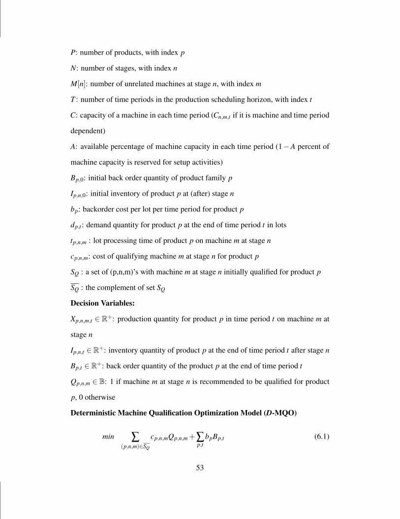
P: number of products, with index p

N: number of stages, with index n

M[n]: number of unrelated machines at stage n, with index m

T : number of time periods in the production scheduling horizon, with index t

C: capacity of a machine in each time period (Cn,m,t if it is machine and time period

dependent)

A: available percentage of machine capacity in each time period (1−A percent of

machine capacity is reserved for setup activities)

Bp,0: initial back order quantity of product family p

Ip,n,0: initial inventory of product p at (after) stage n

bp: backorder cost per lot per time period for product p

dp,t : demand quantity for product p at the end of time period t in lots

tp,n,m : lot processing time of product p on machine m at stage n

cp,n,m: cost of qualifying machine m at stage n for product p

SQ : a set of (p,n,m)’s with machine m at stage n initially qualified for product p

SQ : the complement of set SQ

Decision Variables:

Xp,n,m,t ∈ R+: production quantity for product p in time period t on machine m at

stage n

Ip,n,t ∈ R+: inventory quantity of product p at the end of time period t after stage n

Bp,t ∈ R+: back order quantity of the product p at the end of time period t

Qp,n,m ∈ B: 1 if machine m at stage n is recommended to be qualified for product

p, 0 otherwise

Deterministic Machine Qualification Optimization Model (D-MQO)

min ∑(p,n,m)∈SQ

cp,n,mQp,n,m +∑p,t

bpBp,t (6.1)

53

s.t. Ip,n,t−1 +∑m

Xp,n,m,t −∑m

Xp,n+1,m,t = Ip,n,t , ∀ p,n < N, t (6.2)

Ip,N,t−1 −Bp,t−1 +∑m

Xp,N,m,t −dp,t = Ip,N,t −Bp,t , ∀ p, t (6.3)

∑m

Xp,n+1,m,t ≤ Ip,n,t−1, ∀ p,n < N, t (6.4)

∑p

tp,n,mXp,n,m,t ≤C ·A, ∀ n,1 ≤ m ≤ M[n], t (6.5)

tp,n,mXp,n,m,t ≤CQp,n,m, ∀ p,n,m, t (6.6)

Qp,n,m = 1, ∀ (p,n,m) ∈ SQ (6.7)

Xp,n,m,t , Ip,n,t ,Bp,t ∈ R+, ∀ p,n,m, t (6.8)

Qp,n,m ∈ B, ∀ p,n,m (6.9)

The objective (6.1) is to minimize the total machine qualification and backorder

costs. Constraints (6.2) are the inventory balance constraints for every product at

every stage, except for the last stage, in each time period. They indicate that the

inventory quantity at the end of period t must equal to the beginning inventory

plus production at stage n in period t minus consumption at the next stage n+1 in

period t. Constraints (6.3) are the inventory balance constraints for every product

at the last stage in each time period. They are similar to constraints (6.2) except

that the consumption at the next stage n + 1 in period t is replaced by demand

at the end of period t. Backorders are allowed but incur cumulative backorder

costs as shown in the objective expression (6.1). Constraints (6.4) are the material

availability constraints, which state that the production quantity at stage n in period

t must be less than the inventory quantity at the previous stage n− 1 at the end of

period t − 1. If a lot can flow through more than one stage in one time period, the

RHS’s of constraints (6.4) can be expanded to include production at one or more

prior stages. Constraints (6.5) are the capacity constraints for every machine in

each time period, which state that the total production time over all products must54

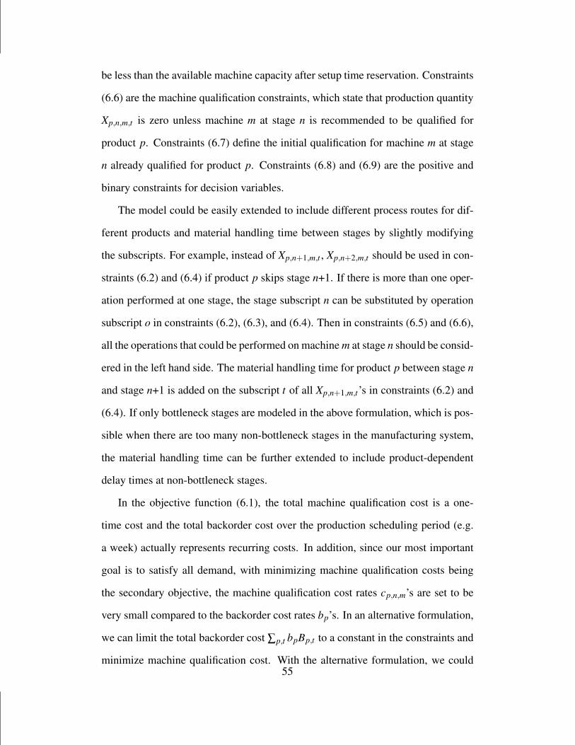
be less than the available machine capacity after setup time reservation. Constraints

(6.6) are the machine qualification constraints, which state that production quantity

Xp,n,m,t is zero unless machine m at stage n is recommended to be qualified for

product p. Constraints (6.7) define the initial qualification for machine m at stage

n already qualified for product p. Constraints (6.8) and (6.9) are the positive and

binary constraints for decision variables.

The model could be easily extended to include different process routes for dif-

ferent products and material handling time between stages by slightly modifying

the subscripts. For example, instead of Xp,n+1,m,t , Xp,n+2,m,t should be used in con-

straints (6.2) and (6.4) if product p skips stage n+1. If there is more than one oper-

ation performed at one stage, the stage subscript n can be substituted by operation

subscript o in constraints (6.2), (6.3), and (6.4). Then in constraints (6.5) and (6.6),

all the operations that could be performed on machine m at stage n should be consid-

ered in the left hand side. The material handling time for product p between stage n

and stage n+1 is added on the subscript t of all Xp,n+1,m,t’s in constraints (6.2) and

(6.4). If only bottleneck stages are modeled in the above formulation, which is pos-

sible when there are too many non-bottleneck stages in the manufacturing system,

the material handling time can be further extended to include product-dependent

delay times at non-bottleneck stages.

In the objective function (6.1), the total machine qualification cost is a one-

time cost and the total backorder cost over the production scheduling period (e.g.

a week) actually represents recurring costs. In addition, since our most important

goal is to satisfy all demand, with minimizing machine qualification costs being

the secondary objective, the machine qualification cost rates cp,n,m’s are set to be

very small compared to the backorder cost rates bp’s. In an alternative formulation,

we can limit the total backorder cost ∑p,t bpBp,t to a constant in the constraints and

minimize machine qualification cost. With the alternative formulation, we could55

generate a tradeoff curve between the total backorder cost limit and the total ma-

chine qualification cost.

The medium-term production scheduling considered in the above formulation

is a snapshot of future production scheduling. Therefore it should reflect a steady

state of the production system. If we start with an empty system in the above

formulation, the start-up effect could give us a non-optimal machine qualification

for future steady state production scheduling. As a result, Little’s law [Little, 1961]

is used to estimate initial inventory quantities in the above formulation in a steady

state system:

Ip,n,0 = tp,n · dp, ∀p,n (6.10)

where Ip,n,0 is the initial inventory of product p at (after) stage n, tp,n is the average

lot processing time of product p at stage n, and dp is the average demand rate of

product p. Average waiting time could be included in tp,n if desired. To keep the

production system in the steady state, the ending inventory quantities at all stages

should be greater than or equal to the corresponding starting inventory quantities or

otherwise defined minimum. Therefore the following constraints should be added

to the formulation during realization.

Ip,n,T ≥ Ip,n,0, ∀p,n (6.11)

In the above deterministic model, the demand quantities dp,t’s used in the pro-

duction scheduling are assumed to be certain at the time when the machine quali-

fication decisions are made. However, the demand quantities are usually based on

forecast and thus uncertain in real world. Therefore, a stochastic model is proposed

in the following section to consider the demand uncertainty.

56

6.3 Stochastic Machine Qualification Optimization Model (S-MQO)

Machine qualification is usually a long term factory configuration decision which

incurs nonnegligible time and monetary costs. It affects capacity allocation and

thus daily production schedules directly. In our model, the machine qualification

decisions are integrated with medium term production scheduling. The objective

is to minimize the total machine qualification costs and backorder costs. Since the

demand data used in the production scheduling are uncertain, a stochastic machine

qualification optimization model is proposed in this section with the objective of

minimizing total machine qualification costs and expected backorder costs. The

purpose of this stochastic model is to find a robust product-machine qualification

matrix at minimal qualification cost. Cost parameters need to be assigned to ma-

chine qualification operations at now and backorders in the future. Those parame-

ters should be determined carefully considering that minimizing backorders is the

primary objective and minimizing qualification costs is the secondary objective.

A two-stage stochastic machine qualification model is presented below. The

demand is represented by a random vector ξ = (d0,0, ...,dP,T )T , with dp,t being

the demand quantity of product p in period t. The objective (6.12) is to minimize

the summation of total machine qualification costs ∑(p,n,m)∈SQcp,n,mQp,n,m and ex-

pected total backorder costs E[O(X , I,B,ξ )] over all possible demand scenarios.

min ∑(p,n,m)∈SQ

cp,n,mQp,n,m +E[O(X , I,B,ξ )] (6.12)

s.t. Qp,n,m = 1, ∀ (p,n,m) ∈ SQ (6.13)

Qp,n,m ∈ B, ∀ p,n,m (6.14)

O(X , I,B,ξ ) is the optimal value of the following production scheduling subprob-

57

lem given a machine qualification matrix Q and a demand scenario ξs:

min ∑p,t

bpBp,t (6.15)

s.t. Ip,n,t−1 +∑m

Xp,n,m,t −∑m

Xp,n+1,m,t = Ip,n,t , ∀ p,n < Np, t (6.16)

Ip,Np,t−1 −Bp,t−1 +∑m

Xp,Np,m,t −dp,t(ξs) = Ip,Np,t −Bp,t , ∀ p, t (6.17)

∑m

Xp,n+1,m,t ≤ Ip,n,t−1, ∀ p,n < Np, t (6.18)

Ip,n,T ≥ Ip,n,0, ∀p,n (6.19)

∑p

tp,n,mXp,n,m,t ≤C ·A, ∀ n,m, t (6.20)

tp,n,mXp,n,m,t ≤CQp,n,m, ∀ p,n,m, t (6.21)

Xp,n,m,t , Ip,n,t ,Bp,t ∈ R+, ∀ p,n,m, t (6.22)

The first-stage decision variables Qp,n,m’s are determined before the realization of

random demand vector ξ . The second-stage decision variables Xp,n,m,t’s, Ip,n,t’s,

and Bp,t’s are determined based on the first-stage decision and the realized demand

vector ξs.

6.4 Deterministic Equivalent Formulation

If the random demand vector ξ can be represented or approximated by a discrete

distribution with possible demand scenarios (ξ1, ...,ξS) and associated probabilities

(P(ξ1), ...,P(ξS)), the previous two-stage stochastic model could be rewritten as the

following deterministic equivalent formulation. Xp,n,m,t(ξs)’s, Ip,n,t(ξs)’s, Bp,t(ξs)’s

are the second-stage decision variables for demand scenario ξs.

min ∑p,t,s

P(ξs)bpBp,t(ξs)+ ∑(p,n,m)∈SQ

cp,n,mQp,n,m (6.23)

s.t. Ip,n,t−1(ξs)+∑m

Xp,n,m,t(ξs)−∑m

Xp,n+1,m,t(ξs) = Ip,n,t(ξs), ∀ p,

n < Np, t,s (6.24)58

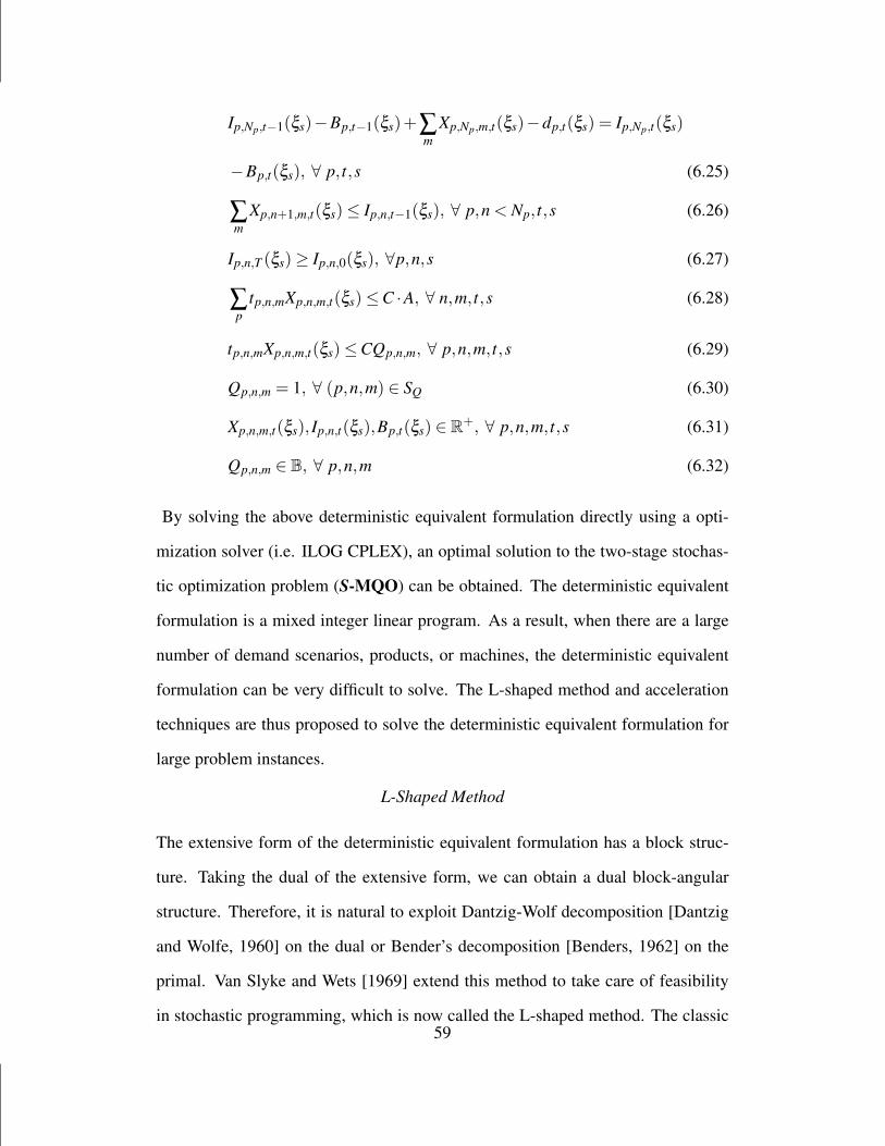
Ip,Np,t−1(ξs)−Bp,t−1(ξs)+∑m

Xp,Np,m,t(ξs)−dp,t(ξs) = Ip,Np,t(ξs)

−Bp,t(ξs), ∀ p, t,s (6.25)

∑m

Xp,n+1,m,t(ξs)≤ Ip,n,t−1(ξs), ∀ p,n < Np, t,s (6.26)

Ip,n,T (ξs)≥ Ip,n,0(ξs), ∀p,n,s (6.27)

∑p

tp,n,mXp,n,m,t(ξs)≤C ·A, ∀ n,m, t,s (6.28)

tp,n,mXp,n,m,t(ξs)≤CQp,n,m, ∀ p,n,m, t,s (6.29)

Qp,n,m = 1, ∀ (p,n,m) ∈ SQ (6.30)

Xp,n,m,t(ξs), Ip,n,t(ξs),Bp,t(ξs) ∈ R+, ∀ p,n,m, t,s (6.31)

Qp,n,m ∈ B, ∀ p,n,m (6.32)

By solving the above deterministic equivalent formulation directly using a opti-

mization solver (i.e. ILOG CPLEX), an optimal solution to the two-stage stochas-

tic optimization problem (S-MQO) can be obtained. The deterministic equivalent

formulation is a mixed integer linear program. As a result, when there are a large

number of demand scenarios, products, or machines, the deterministic equivalent

formulation can be very difficult to solve. The L-shaped method and acceleration

techniques are thus proposed to solve the deterministic equivalent formulation for

large problem instances.

L-Shaped Method

The extensive form of the deterministic equivalent formulation has a block struc-

ture. Taking the dual of the extensive form, we can obtain a dual block-angular

structure. Therefore, it is natural to exploit Dantzig-Wolf decomposition [Dantzig

and Wolfe, 1960] on the dual or Bender’s decomposition [Benders, 1962] on the

primal. Van Slyke and Wets [1969] extend this method to take care of feasibility

in stochastic programming, which is now called the L-shaped method. The classic59

L-shaped method is first developed only for stochastic linear programs. A valid

set of feasibility cuts and optimality cuts is known to exist in the continuous case,

based on duality theory in linear programming. This knowledge forms the basis

of the classic L-shaped method. Those cuts can also be used in the case where

only some first-stage variables are integers, e.g. the S-MQO model. On the other

hand, properties of general integer stochastic programs are scarce, and there is an

absence of general efficient solution methods. The integer L-shaped method is the

integration of the classic L-shaped method and branch-and-bound, during which

optimality and feasibility cuts are added to LP relaxations. Since the S-MQO has

binary first-stage variables and continuous second-stage variables, the classic L-

shaped decomposition algorithm is chosen instead of the integer L-shaped method.

The L-shaped method is briefly described below as it applies to our problem.

L-Shaped Method

Step 0 Set lower bound LB=−∞ and upper bound UB=∞. Set the iteration count

i = 0.

Step 1 Solve the master problem for an optimal solution Qi

LB = min ∑(p,n,m)∈SQ

cp,n,mQp,n,m +θ

s.t. Qp,n,m = 1, ∀ (p,n,m) ∈ SQ

Qp,n,m ∈ B, ∀ p,n,m

θ ≥ ∑p,n,m

Ekp,n,mQp,n,m + ek,k = 1,2, ..., i

Step 2 For s = 1, ...,S, solve the following subproblem corresponding to Qi and ξs

O(Qi,ξs) = min ∑p,t

bpBp,t Dual

60

s.t. Ip,n,0 +∑m

Xp,n,m,1 −∑m

Xp,n+1,m,1 = Ip,n,1,∀ p,n < Np (γp,n(ξs))

Ip,n,t−1 +∑m

Xp,n,m,t −∑m

Xp,n+1,m,t = Ip,n,t ,∀ p,n < Np,

1 < t ≤ T

Ip,Np,t−1 −Bp,t−1 +∑m

Xp,Np,m,t −dp,t(ξs) = Ip,Np,t −Bp,t ,

∀ p, t (µp,t(ξs))

∑m

Xp,n+1,m,1 ≤ Ip,n,0, ∀ p,n < Np (σp,n(ξs))

∑m

Xp,n+1,m,t ≤ Ip,n,t−1, ∀ p,n < Np,1 < t ≤ T

Ip,n,T ≥ Ip,n,0, ∀p,n (φp,n(ξs))

∑p

tp,n,mXp,n,m,t ≤C ·A, ∀ n,m, t (πn,m,t(ξs))

tp,n,mXp,n,m,t ≤CQip,n,m, ∀ p,n,m, t (ρp,n,m,t(ξs))

Xp,n,m,t , Ip,n,t ,Bp,t ∈ R+, ∀ p,n,m, t

If ∑(p,n,m)∈SQcp,n,mQi

p,n,m+∑s P(ξs)O(Qi,ξs)<UB, update the upper bound.

Step 3 If (UB−LB)/LB < δ , stop and return Q = {Qip,n,m} as the optimal solution

and UB as the optimal objective value.

Step 4 For each s = 1,2, ...,S, compute the cut coefficients

E i+1p,n,m = ∑

sP(ξs)(∑

tρp,n,m,t(ξs) ·Cn,m,t)

and

ei+1 =∑s

P(ξs)[− ∑p,n<Np

Ip,n,0 · γp,n(ξs)+ ∑p,n<Np

Ip,n,0 ·∑p,t

σp,n(ξs)

+∑p,n

Ip,n,0 ·φp,n(ξs)+∑p

µp,1(ξs) · (dp,1(ξs)− Ip,Np,0)

+ ∑p,t>1

µp,t(ξs) ·dp,t(ξs)+ ∑n,m,t

πn,m,t(ξs) ·C ·A].

61

Update i = i+1 and go to Step 1.

In the L-shaped method, the master program solved in Step 1 provides a lower

linear approximation for the function ∑s P(ξs)O(Q,ξs) through a continuous vari-

able θ and optimality cuts θ ≥∑p,n,m Ekp,n,mQp,n,m+ek, and therefore a lower bound

LB for the objective function (6.23). The optimal solution Qi obtained through the

master program corresponds to a feasible solution for the stochastic program. It

should be noted that in the first iteration i = 0, neither θ nor any optimality cut

is included in the master problem. In Step 2, all S subproblems are solved us-

ing the optimal Qi obtained from the master problem and corresponding demand

scenario ξs. These S linear programs are solved independently, allowing for a com-

putationally convenient decomposition. If all S subproblems are feasible, which in

our case is always true since backorders are allowed in all subproblems, these sub-

problem solutions together with the master problem solution yield a upper bound

UB of the original problem. When the upper bound UB and the lower bound LB

are sufficiently close within a preset relative error term δ , we conclude optimality.

Otherwise the dual optimal solutions of the subproblems are used to compute an op-

timality cut added in the master program in the next iteration. Only dual variables

corresponding to constraints with positive right-hand-side values or positive coeffi-

cients of first-stage variables (Qp,n,m’s) will affect the cut coefficients. Those dual

variables are represented as the γp,n’s, µp,t’s, σp,n’s, πn,m,t’s, φp,n’s, and ρp,n,m,t’s

in the parenthesis. It should be noted that the initial inventory quantities Ip,Np,0’s

at/after the last stage are assumed to be zero, because the demand quantities Bp,t’s

can always be adjusted to make Ip,Np,0’s zero. In Step 4, according to the duality

theory the optimality cut ∑s P(ξs)O(Q,ξs) = E i+1p,n,mQp,n,m+ei+1 is exact for Qi and

is a lower linear approximate for all other feasible Q’s.

62

In the classic L-shaped method, two types of cuts are added to the master prob-

lem: feasibility cuts and optimality cuts. Optimality cuts are computed in the previ-

ous algorithm in Step 4. Feasibility cuts are added if and only if the master solution

in Step 1 is infeasible for certain subproblems in Step 2. Since backorders are al-

lowed in our model, all feasible master problem solutions are feasible for all the

subproblems. As a result, no feasibility cut is added in the algorithm.

Acceleration of The L-Shaped Method

The number of iterations in the L-shaped method for real world problem instances

can be very large. To improve the convergence behavior of the L-shaped method,

the following acceleration techniques are proposed.

Cut Disaggregation

In the standard L-shaped method, one optimality cut is added at each iteration,

which approximates the expectation of the second-stage objective functions given

the current first-stage solution. Instead of one cut, S optimality cuts could be added

at each iteration to approximate individual second-stage objective functions. The

optimality cut corresponding to demand scenario ξs at iteration i is represented by

θ s ≥ ∑p,n,m

Es,ip,n,mQp,n,m + es,i,

in which

Es,ip,n,m = ∑

tρ i

p,n,m,t(ξs) ·Cn,m,t

and

es,i =− ∑p,n<Np

Ip,n,0 · γ ip,n(ξs)+ ∑

p,n<Np

Ip,n,0 ·∑p,t

σ ip,n(ξs)

+∑p,n

Ip,n,0 ·φ ip,n(ξs)+∑

pµ i

p,1(ξs) · (dp,1(ξs)− Ip,Np,0)

+ ∑p,t>1

µ ip,t(ξs) ·dp,t(ξs)+ ∑

n,m,tπ i

n,m,t(ξs) ·C ·A.

63

In the (i+1)th iteration, the master problem takes the following form.

min ∑(p,n,m)∈SQ

cp,n,mQp,n,m +∑s

P(ξs)θ s

s.t. Qp,n,m = 1, ∀ (p,n,m) ∈ SQ

Qp,n,m ∈ B, ∀ p,n,m

θ s ≥ ∑p,n,m

Es,ip,n,mQp,n,m + es,i,k = 1,2, ..., i,s = 1,2, ...,S

This approach is referred to as multicut L-shaped algorithm [Birge Francois and

John, 1988]. In the multicut version, there is no information loss due to cut ag-

gregation, thus providing a better approximation of the expectation of second-stage

objective functions. Consequently, there are fewer iterations in the multicut L-

shaped method. However, since more cuts are added at each iteration, the cost of

the multicut algorithm is to solve larger master problems.

Qualification Cuts

In the early iterations of the standard L-shaped method there are very few cuts

in the master problem. As a result, a minimal number of machines are qualified

in the optimal solutions of the master problem, which results in large backorder

quantities at the second-stage subproblems. To avoid such poor master problem

solutions, information of the second-stage subproblems is integrated in the master

problem. Qualification cuts are added in the master problem to impose a lower

bound restriction on the number of machines to be qualified for each product at

each stage.

The following formulation is defined as the single-scenario qualification sub-

problem for ξs (1 ≤ s ≤ S).

min P(ξs)∑p,t

bpBp,t(ξs)+ ∑(p,n,m)∈SQ

cp,n,mQp,n,m(ξs)

s.t. Ip,n,t−1(ξs)+∑m

Xp,n,m,t(ξs)−∑m

Xp,n+1,m,t(ξs) = Ip,n,t(ξs), ∀ p,n < Np, t

64

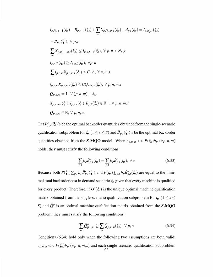
Ip,Np,t−1(ξs)−Bp,t−1(ξs)+∑m

Xp,Np,m,t(ξs)−dp,t(ξs) = Ip,Np,t(ξs)

−Bp,t(ξs), ∀ p, t

∑m

Xp,n+1,m,t(ξs)≤ Ip,n,t−1(ξs), ∀ p,n < Np, t

Ip,n,T (ξs)≥ Ip,n,0(ξs), ∀p,n

∑p

tp,n,mXp,n,m,t(ξs)≤C ·A, ∀ n,m, t

tp,n,mXp,n,m,t(ξs)≤CQp,n,m(ξs), ∀ p,n,m, t

Qp,n,m = 1, ∀ (p,n,m) ∈ SQ

Xp,n,m,t(ξs), Ip,n,t(ξs),Bp,t(ξs) ∈ R+, ∀ p,n,m, t

Qp,n,m ∈ B, ∀ p,n,m

Let Bsp,t(ξs)’s be the optimal backorder quantities obtained from the single-scenario

qualification subproblem for ξs (1 ≤ s ≤ S) and Bop,t(ξs)’s be the optimal backorder

quantities obtained from the S-MQO model. When cp,n,m << P(ξs)bp (∀p,n,m)

holds, they must satisfy the following conditions:

∑p,t

bpBsp,t(ξs) = ∑

p,tbpBo

p,t(ξs), ∀ s (6.33)

Because both P(ξs)∑p,t bpBsp,t(ξs) and P(ξs)∑p,t bpBo

p,t(ξs) are equal to the mini-

mal total backorder cost in demand scenario ξs given that every machine is qualified

for every product. Therefore, if Qs(ξs) is the unique optimal machine qualification

matrix obtained from the single-scenario qualification subproblem for ξs (1 ≤ s ≤

S) and Qo is an optimal machine qualification matrix obtained from the S-MQO

problem, they must satisfy the following conditions:

∑m

Qop,n,m ≥ ∑

mQs

p,n,m(ξs), ∀ p,n (6.34)

Conditions (6.34) hold only when the following two assumptions are both valid:

cp,n,m << P(ξs)bp (∀p,n,m,s) and each single-scenario qualification subproblem65

has a unique optimal machine qualification matrix. The first assumption cp,n,m <<

P(ξs)bp (∀p,n,m,s) holds if the cost parameters cp,n,m’s and bp’s are carefully cho-

sen. Because there are usually multiple optimal solutions for real world applica-

tions, the second assumption usually does not hold. As a result, adding inequal-

ities (6.34) in the master problem leads to a sub-optimal solution for the original

S-MQO problem. However, if the first assumption holds, the expected total back-

order costs over all scenarios should still be the same with or without inequalities

(6.34). Adding inequalities (6.34) will decrease the number of iterations in the L-

shaped method. Thus the tradeoff here is between the total machine qualification

cost and the solution time of L-shaped method. Inequalities (6.34) are referred to

as qualification cuts in this paper.

Relaxed Qualification Cuts

When the problem size increases, even the single-scenario qualification sub-

problem can be difficult to solve since it is a mixed integer linear program. In this

case, we can solve the LP relaxation of the single-scenario qualification subproblem

for an optimal continuous machine qualification matrix Qs. Then a binary machine

qualification ¯Qs can be obtained using the following rule:¯Qs = 1, Qs > ε¯Qs = 0, Qs ≤ ε

where ε is a preset value between 0 and 1. A set of qualification cuts similar to in-

equalities (6.34) can be added using ¯Qs instead of Qs. Those cuts are called relaxed

qualification cuts. They require significantly less time for solving the (relaxed)

single-scenario qualification subproblems. On the other hand, both optimal ma-

chine qualification cost and expected backorder cost with relaxed qualification cuts

can be larger than those of the original S-MQO problem. Therefore, the tradeoff

here is still between the solution quality and solution time.

66

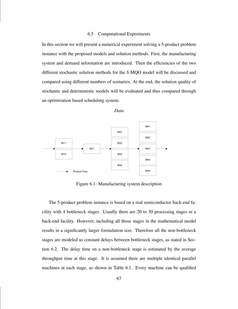
6.5 Computational Experiments

In this section we will present a numerical experiment solving a 5-product problem

instance with the proposed models and solution methods. First, the manufacturing

system and demand information are introduced. Then the efficiencies of the two

different stochastic solution methods for the S-MQO model will be discussed and

compared using different numbers of scenarios. At the end, the solution quality of

stochastic and deterministic models will be evaluated and thus compared through

an optimization based scheduling system.

Data

M21

M41

M42

M43

M44

M45

M31

M32

M33

M34

M11

M12

Product Flow

Figure 6.1: Manufacturing system description

The 5-product problem instance is based on a real semiconductor back-end fa-

cility with 4 bottleneck stages. Usually there are 20 to 30 processing stages in a

back-end facility. However, including all those stages in the mathematical model

results in a significantly larger formulation size. Therefore all the non-bottleneck

stages are modeled as constant delays between bottleneck stages, as stated in Sec-

tion 6.2. The delay time on a non-bottleneck stage is estimated by the average

throughput time at this stage. It is assumed there are multiple identical parallel

machines at each stage, as shown in Table 6.1. Every machine can be qualified

67

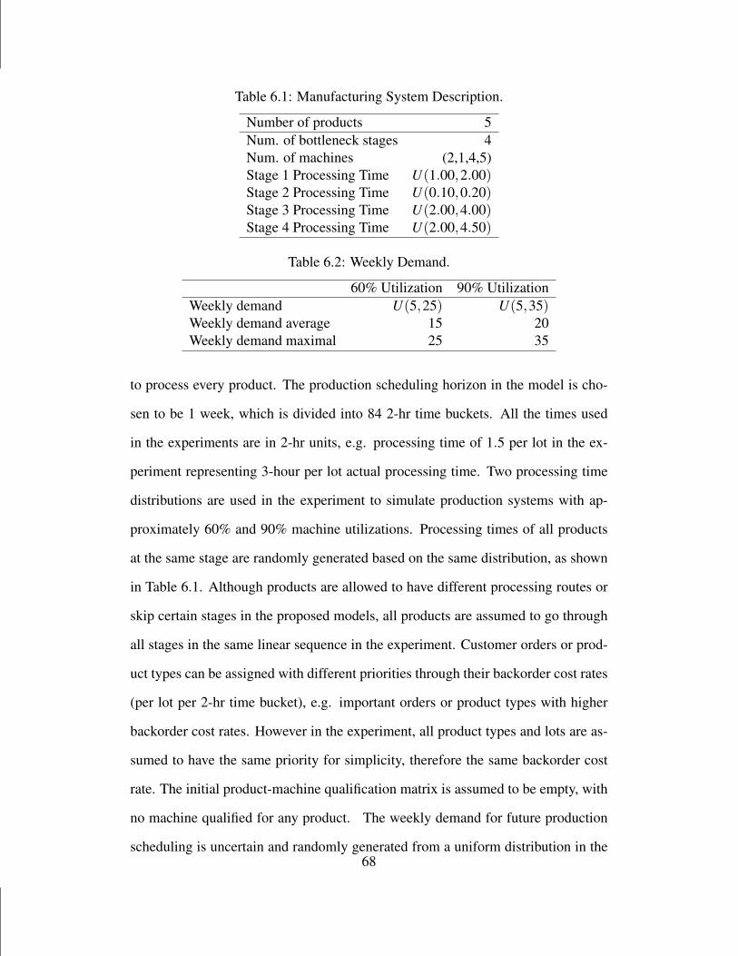
Table 6.1: Manufacturing System Description.

Number of products 5Num. of bottleneck stages 4Num. of machines (2,1,4,5)Stage 1 Processing Time U(1.00,2.00)Stage 2 Processing Time U(0.10,0.20)Stage 3 Processing Time U(2.00,4.00)Stage 4 Processing Time U(2.00,4.50)

Table 6.2: Weekly Demand.

60% Utilization 90% UtilizationWeekly demand U(5,25) U(5,35)Weekly demand average 15 20Weekly demand maximal 25 35

to process every product. The production scheduling horizon in the model is cho-

sen to be 1 week, which is divided into 84 2-hr time buckets. All the times used

in the experiments are in 2-hr units, e.g. processing time of 1.5 per lot in the ex-

periment representing 3-hour per lot actual processing time. Two processing time

distributions are used in the experiment to simulate production systems with ap-

proximately 60% and 90% machine utilizations. Processing times of all products

at the same stage are randomly generated based on the same distribution, as shown

in Table 6.1. Although products are allowed to have different processing routes or

skip certain stages in the proposed models, all products are assumed to go through

all stages in the same linear sequence in the experiment. Customer orders or prod-

uct types can be assigned with different priorities through their backorder cost rates

(per lot per 2-hr time bucket), e.g. important orders or product types with higher

backorder cost rates. However in the experiment, all product types and lots are as-

sumed to have the same priority for simplicity, therefore the same backorder cost

rate. The initial product-machine qualification matrix is assumed to be empty, with

no machine qualified for any product. The weekly demand for future production

scheduling is uncertain and randomly generated from a uniform distribution in the68

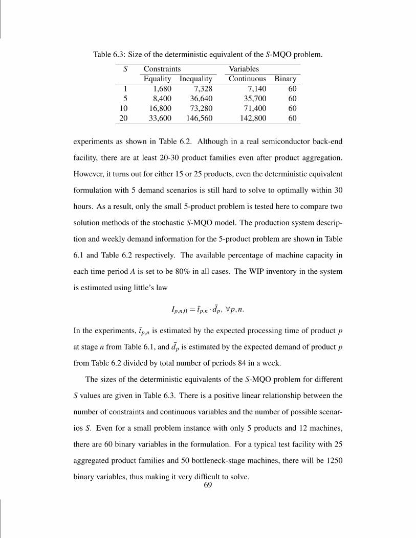
Table 6.3: Size of the deterministic equivalent of the S-MQO problem.

S Constraints VariablesEquality Inequality Continuous Binary

1 1,680 7,328 7,140 605 8,400 36,640 35,700 60

10 16,800 73,280 71,400 6020 33,600 146,560 142,800 60

experiments as shown in Table 6.2. Although in a real semiconductor back-end

facility, there are at least 20-30 product families even after product aggregation.

However, it turns out for either 15 or 25 products, even the deterministic equivalent

formulation with 5 demand scenarios is still hard to solve to optimally within 30

hours. As a result, only the small 5-product problem is tested here to compare two

solution methods of the stochastic S-MQO model. The production system descrip-

tion and weekly demand information for the 5-product problem are shown in Table

6.1 and Table 6.2 respectively. The available percentage of machine capacity in

each time period A is set to be 80% in all cases. The WIP inventory in the system

is estimated using little’s law

Ip,n,0 = tp,n · dp, ∀p,n.

In the experiments, tp,n is estimated by the expected processing time of product p

at stage n from Table 6.1, and dp is estimated by the expected demand of product p

from Table 6.2 divided by total number of periods 84 in a week.

The sizes of the deterministic equivalents of the S-MQO problem for different

S values are given in Table 6.3. There is a positive linear relationship between the

number of constraints and continuous variables and the number of possible scenar-

ios S. Even for a small problem instance with only 5 products and 12 machines,

there are 60 binary variables in the formulation. For a typical test facility with 25

aggregated product families and 50 bottleneck-stage machines, there will be 1250

binary variables, thus making it very difficult to solve.69

Performance of Different Solution Methods

In the experiment, two different solution methods for the S-MQO model are tested.

One is to solve the deterministic equivalent formulation (DE). The other is the L-

shaped method (Bender). Proposed acceleration techniques of the L-shaped method

are also tested, including cut disaggregation (CD), qualification cuts (QC), and re-

laxed qualification cuts (RQC). Solution times of all tested solution methods are

ploted in Figure 6.2 for different S values and machine utilizations. More details

about the solution times of different methods are shown in Table 6.4, including

solution/decomposition (BD) time, time for adding qualification cuts before the de-

composition (QC time), number of iterations in the decomposition algorithm, and

optimality gap at the end of runtime limit (36000 sec). L-shaped method with

cut disaggregation and relaxed qualification cuts (“Bender + CD + RQC”) has the

shortest solution times and fewest numbers of iterations. L-shaped method with

cut disaggregation and qualification cuts (“Bender + CD + QC”) has relatively few

numbers of iterations but the unstable solution times. It is also noted that the time

required for solving single-scenario qualification subproblems (QC time) increases

significantly when S increases. As a result, adding qualification cuts is not suitable

for real size problem instances. L-shaped method with cut disaggregation (“Bender

+ CD”) has relatively short solution times but relatively large numbers of iterations,

which could make it unsuitable for real size problem instances either. All other

solution methods have both long solution times and larger number of iterations.

The quality of solutions of different methods are listed in Table 6.5 for different

S values and machine utilizations. Optimal solutions obtained with the first two

methods are also optimal to the original S-MQO model. However, optimal solu-

tions obtained with the last four methods can be sub-optimal to the original S-MQO

model, due to QC/RQC cuts. Both the total qualification costs and the expected to-

70

tal backorder costs are shown in the “Q cost” and “B cost” columns respectively in

Table 6.5. In the experiment, cp,n,m = 0.1 (∀ p,n,m) and bp = 1 (∀ p). From “Ben-

der + CD” to “Bender + QC” or “Bender + CD + QC”, the optimal “B cost” does

not increase, and the optimal “Q cost” and “Total cost” increase slightly. For “Ben-

der + RQC” and “Bender + CD + RQC”, the optimal “B cost”, “Q cost” and “Total

cost” all increase. This is consistent with the previous analysis. The increase in “B

cost” for “Bender + RQC” and “Bender + CD + RQC” is significant when S is 20.

The reason is that cp,n,m < P(ξs)bp does not hold anymore when S is 20. Therefore,

cp,n,m’s and bp’s should be chosen carefully to make sure that cp,n,m < P(ξs)bp is

valid if “Bender + CD + QC” is to be implemented. “Bender + CD + RQC” and

“Bender + CD” are recommended for large size problem instances because of short

solution times and small numbers of iterations. If ”Bender + CD” does not find

the optimal solution and ”Bender + CD + RQC” finds one, thus providing an upper

bound of the S-MQO model, a lower bound can be estimated by the LP relaxation

of the original S-MQO problem.

At the end, the optimal qualification matrices obtained using the L-shaped method

with cut disaggregation for different S values and machine utilizations are evaluated

using a different set of 20 demand scenarios generated according to the distributions

in Table 6.2. Each demand scenarios is given an equal probability of 0.05. A pro-

duction scheduling linear program is solved for each demand scenario and each

optimal qualification matrix. The total qualification cost and expected total back-

order cost for each optimal qualification matrix are listed in the ”Q cost” and ”B

cost” columns of Table 6.6. Optimal qualification matrices from the deterministic

model using the average or maximal demand are listed in the first and second row.

For both 60% and 90% machine utilization cases, the optimal qualification matrices

obtained from the stochastic model outperform those obtained from the determin-

istic model. For the stochastic model, the optimal qualification matrix obtained71

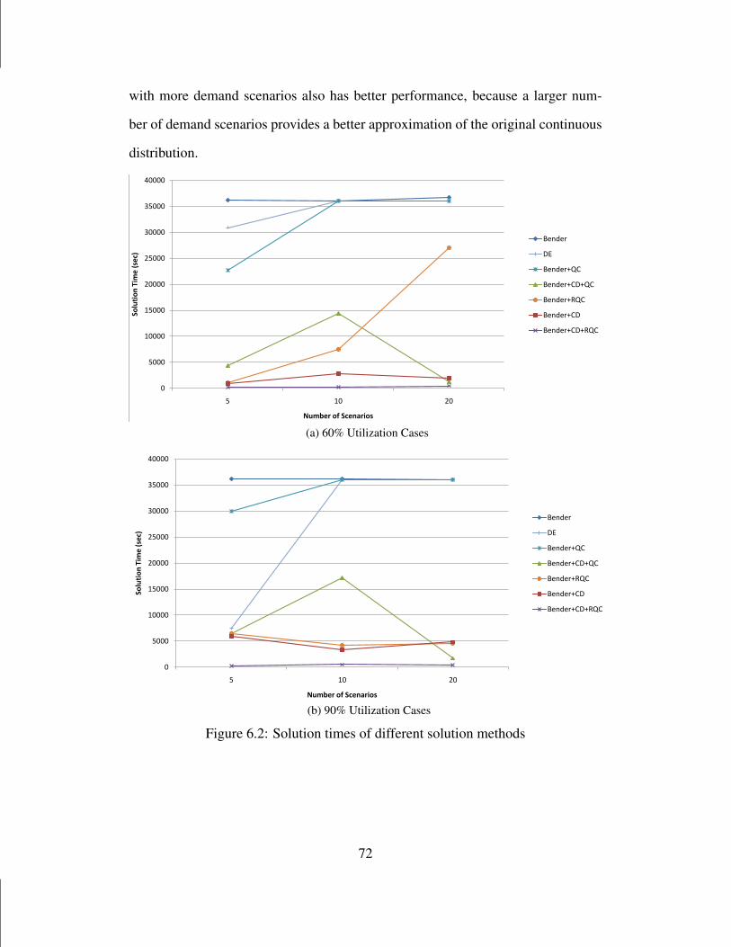
with more demand scenarios also has better performance, because a larger num-

ber of demand scenarios provides a better approximation of the original continuous

distribution.

0

5000

10000

15000

20000

25000

30000

35000

40000

5 10 20

So

luti

on

Tim

e (

sec)

Number of Scenarios

Bender

DE

Bender+QC

Bender+CD+QC

Bender+RQC

Bender+CD

Bender+CD+RQC

(a) 60% Utilization Cases

0

5000

10000

15000

20000

25000

30000

35000

40000

5 10 20

So

luti

on

Tim

e (

sec)

Number of Scenarios

Bender

DE

Bender+QC

Bender+CD+QC

Bender+RQC

Bender+CD

Bender+CD+RQC

(b) 90% Utilization Cases

Figure 6.2: Solution times of different solution methods

72

Tabl

e6.

4:So

lutio

ntim

eco

mpa

riso

nof

diff

eren

tacc

eler

atio

nm

etho

ds.

S=

560

%U

tiliz

atio

n90

%U

tiliz

atio

nB

Dtim

eQ

Ctim

eIt

erat

ions

Gap

BD

time

QC

time

Iter

atio

nsG

ap(s

ec)

(sec

)(%

)(s

ec)

(sec

)(%

)B

ende

r36

147

524

4136

143

605

11B

ende

r+C

D89

319

70

5919

452

0B

ende

r+Q

C22

750

3837

2494

030

006

4960

2019

2B

ende

r+C

D+

QC

4315

3819

800

6534

4965

950

Ben

der+

RQ

C10

643

200

064

915

516

0B

ende

r+C

D+

RQ

C17

73

280

244

412

0S=

1060

%U

tiliz

atio

n90

%U

tiliz

atio

nB

Dtim

eQ

Ctim

eIt

erat

ions

Gap

BD

time

QC

time

Iter

atio

nsG

ap(s

ec)

(sec

)(%

)(s

ec)

(sec

)(%

)B

ende

r36

122

349

6136

168

755

17B

ende

r+C

D28

5518

30

3326

161

0B

ende

r+Q

C36

012

1377

919

0731

3601

516

290

803

2B

ende

r+C

D+

QC

1440

713

764

550

1717

616

286

380

Ben

der+

RQ

C75

244

613

042

355

228

0B

ende

r+C

D+

RQ

C22

56

180

506

619

0S=

2060

%U

tiliz

atio

n90

%U

tiliz

atio

nB

Dtim

eQ

Ctim

eIt

erat

ions

Gap

BD

time

QC

time

Iter

atio

nsG

ap(s

ec)

(sec

)(%

)(s

ec)

(sec

)(%

)B

ende

r36

751

454

3836

067

314

67B

ende

r+C

D19

2412

60

4826

182

0B

ende

r+Q

C36

018

4931

514

2629

3603

126

783

706

8B

ende

r+C

D+

QC

1246

5015

849

017

1926

813

330

Ben

der+

RQ

C26

998

494

60

4561

713

40

Ben

der+

CD

+R

QC

450

417

038

76

110

73

Tabl

e6.

5:So

lutio

nqu

ality

com

pari

son

ofdi

ffer

enta

ccel

erat

ion

met

hods

.

S=

560

%U

tiliz

atio

n90

%U

tiliz

atio

nQ

cost

Bco

stTo

talc

ost

Gap

(%)

Qco

stB

cost

Tota

lcos

tG

ap(%

)B

ende

r2

4.2

6.2

414.

017

.321

.311

Ben

der+

CD

2.1

2.6

4.7

02.

617

.319

.90

Ben

der+

QC

2.1

2.6

4.7

02.

517

.720

.22

Ben

der+

CD

+Q

C2.

12.

64.

70

2.7

17.4

20.1

0B

ende

r+R

QC

2.3

2.5

4.8

02.

817

.520

.30

Ben

der+

CD

+R

QC

2.3

2.6

4.9

02.

818

.221

.00

S=

1060

%U

tiliz

atio

n90

%U

tiliz

atio

nQ

cost

Bco

stTo

talc

ost

Gap

(%)

Qco

stB

cost

Tota

lcos

tG

ap(%

)B

ende

r5.

80.

96.

761

4.6

12.5

17.1

17B

ende

r+C

D2.

30.

93.

20

2.8

12.7

15.5

0B

ende

r+Q

C3.

60.

94.

531

3.0

12.6

15.6

2B

ende

r+C

D+

QC

2.3

0.9

3.2

02.

912

.615

.50

Ben

der+

RQ

C2.

40.

93.

30

312

.715

.70

Ben

der+

CD

+R

QC

2.4

0.9

3.3

03.

312

.816

.10

S=

2060

%U

tiliz

atio

n90

%U

tiliz

atio

nQ

cost

Bco

stTo

talc

ost

Gap

(%)

Qco

stB

cost

Tota

lcos

tG

ap(%

)B

ende

r3.

50.

74.

238

4.5

12.4

16.9

67B

ende

r+C

D2.

30.

83.

10

2.7

11.7

14.4

0B

ende

r+Q

C3.

21.

14.

329

3.1

11.6

14.7

8B

ende

r+C

D+

QC

2.5

0.7

3.2

03

11.5

14.5

0B

ende

r+R

QC

2.4

0.8

3.2

03.

117

.420

.50

Ben

der+

CD

+R

QC

2.4

0.9

3.3

03.

317

.420

.70

74

Table 6.6: Evaluation of different qualification matrices.

S 60% Utilization 90% UtilizationQ cost B cost Q cost B cost

1 (avg) 2 8.4 2.2 17.51 (max) 1.7 16.3 1.9 39.4

5 2.1 5.5 2.6 16.310 2.3 2.8 2.8 14.920 2.3 2.9 2.7 14.2

6.6 Summary

In this chapter, a stochastic mixed integer linear programming model (S-MQO) is

proposed to optimize product-machine qualifications for a semiconductor back-end

facility. Future production scheduling in a medium term with demand uncertainty is

considered. Setup times are modeled indirectly. The L-shaped method and several

acceleration techniques are proposed to solve the stochastic model. In the numerical

experiment, a 5-product example is used to evaluate different solution methods and

their solutions.

In this research, it is assumed that product-machine qualification decisions are

made and implemented now for a foreseeable future with stationary demand. The

models described could be readily expanded to include time-phased qualification

decisions. An interesting topic for future research will be a multi-stage stochastic

model for time-phased qualification decisions.

75

CHAPTER 7

CONCLUSION

This research is an effort to discuss and fill the gap between theoretical flexible

flow shop scheduling models and real world scheduling problems. An novel opti-

mization model is proposed to schedule a general flexible flow shop with flexible

processing routes, product family related sequence-independent setups, product-

machine qualifications, and customized rules for a semiconductor back-end facility.

However, since the problem itself is NP-hard and the formulation size becomes too

large for real size problem instances, the model can not be solved directly for an

optimal solution in a reasonable time for a real back-end facility. In order to obtain

a “good” schedule in a reasonable time and also include more existing customized

rules/constraints in the back-end process, a deterministic scheduling system is de-

veloped and realized. The deterministic scheduling system is able to integrate ten-

tative production plans and schedule each lot on each individual machine subject to

recourse availability and scheduling rules. Small problem instances are randomly

generated, and solutions from the optimization model and the DSS are compared

regarding solution time and quality (measured by total backorder costs). Based on

the computational experiment results, the DSS is able to provide high quality pro-

duction schedules within a short time. However, quality of the DSS solutions varies

depending on the configuration of the scheduling rules used in the DSS. The DSS

solutions used in the previous experiment are the best solutions among all tested

configurations. Experimental design is applied to understand the behavior of the

deterministic scheduling system with different configurations and provide insights

about schedule rules to be used under different scenarios in the future. In conclu-

sion, the proposed optimization model offers a novel way of modeling a flexible

flow shop with more flexibility and realistic details. On the other hand, the DSS

provides a framework in which more customized rules/constraints and scheduling

rules can be guided by a tentative production plan. The tentative production plan

provides tentative deadlines for each batch at each stage to minimize total backorder

costs while local scheduling rules are used to minimize setups. Both the optimiza-

tion model and the DSS can be applied to other production systems with a similar

structure.

As a production system configuration parameter which has significant and long-

term impact on daily production scheduling in the future, the product-machine qual-

ification matrix is studied in more detail in this research. A stochastic optimization

model is proposed to find a robust product-machine qualification matrix with min-

imal machine qualification costs. The L-shaped method is used to decompose and

solve the deterministic equivalent iteratively. Cuts are developed to decrease the

number of iterations in the solution process and the solution time. Computational

results are provided to justify the necessity of the stochastic model and compare

different solution methods of the stochastic model. The basic idea behind this

product-machine qualification optimization model can be applied to some other

qualification problems, such as employee training, machine purchase, etc.

77

REFERENCESA. Agnetis, A. Pacifici, F. Rossi, M. Lucertini, S. Nicoletti, F. Nicolo, G. Oriolo,

D. Pacciarelli, and E. Pesaro. Scheduling of flexible flow lines in an automo-bile assembly plant. European Journal of Operational Research, 97(2):348–362,1997.

A. Allahverdi, CT Ng, TCE Cheng, and M.Y. Kovalyov. A survey of schedulingproblems with setup times or costs. European Journal of Operational Research,187(3):985–1032, 2008.

C. Andres, J.M. Albarracin, G. Tormo, E. Vicens, and J.P. Garcia-Sabater. Grouptechnology in a hybrid flowshop environment: A case study. European Journalof Operational Research, 167(1):272–281, 2005.

A. Aubry, A. Rossi, M.L. Espinouse, and M. Jacomino. Minimizing setup costsfor parallel multi-purpose machines under load-balancing constraint. EuropeanJournal of Operational Research, 187(3):1115–1125, 2008.

J.F. Benders. Partitioning procedures for solving mixed-variables programmingproblems. Numerische Mathematik, 4(1):238–252, 1962.

V. Birge Francois and R. John. A multicut algorithm for two-stage stochastic linearprograms. European Journal of Operational Research, 34(3):384–392, 1988.

V. Botta-Genoulaz. Hybrid flow shop scheduling with precedence constraints andtime lags to minimize maximum lateness. International Journal of ProductionEconomics, 64(1-3):101–111, 2000.

K.E. Bourland and L.K. Carl. Parallel-machine scheduling with fractional operatorrequirements. IIE Transactions, 26(5):56–65, 1994.

SA Brah and JL Hunsucker. Branch and bound algorithm for the flow shop withmultiple processors. European journal of operational research, 51(1):88–99,1991.

K. Brockmann and W. Dangelmaier. A parallel branch bound algorithm formakespan optimal sequencing in flow shops with parallel machines. In Proc. 2ndIMACS International Multiconference on Computational Engineering in SystemsApplications, pages 431–436, 1997.

K. Brockmann, W. Dangelmaier, and N. Holthofer. Parallel branch bound algorithmfor makespan optimal scheduling in flow shops with multiple processors. InOperations research proceedings 1997: selected papers of the Symposium onOperations Research (SOR’97), Jena, September 3-5, 1997, page 428. Springer,1998.

P. Brucker, B. Jurisch, and A. Kramer. Complexity of scheduling problems withmulti-purpose machines. Annals of Operations Research, 70:57–73, 1997.

G.M. Campbell. Using short-term dedication for scheduling multiple productson parallel machines. Production and Operations Management, 1(3):295–307,1992.

J. Carlier and E. Neron. An exact method for solving the multi-processor flow-shop.RAIRO Operations Research, 34:1–25, 2000.

T.C.E. Cheng, J.N.D. Gupta, and G. Wang. A review of flowshop scheduling re-search with setup times. Production and Operations Management, 9(3):262–282,2000.

D.M. Chiang, R.S. Guo, and F.Y. Pai. Improved customer satisfaction with a hybriddispatching rule in semiconductor back-end factories. International Journal ofProduction Research, 46(17):4903–4923, 2008.

G.B. Dantzig and P. Wolfe. Decomposition principle for linear programs. Opera-tions research, 8(1):101–111, 1960.

S. Dauzere-Peres and J. Paulli. An integrated approach for modeling and solving thegeneral multiprocessor job-shop scheduling problem using tabu search. Annalsof Operations Research, 70:281–306, 1997.

F.Y. Ding and D. Kittichartphayak. Heuristics for scheduling flexible flow lines.Computers and Industrial Engineering, 26(1):27–34, 1994.

A. Drexl and M. Mundschenk. Long-term staffing based on qualification profiles.Mathematical Methods of Operations Research, 68(1):21–47, 2008.

RL Graham. Bounds on multiprocessing timing anomalies. SIAM Journal on Ap-plied Mathematics, 17(2):416–429, 1969.

AGP Guinet and MM Solomon. Scheduling hybrid flowshops to minimize maxi-mum tardiness or maximum completion time. International journal of produc-tion research, 34(6):1643–1654, 1996.

J.N.D. Gupta. Two-stage, hybrid flowshop scheduling problem. Journal of theOperational Research Society, pages 359–364, 1988.

J.N.D. Gupta, K. Kruger, V. Lauff, F. Werner, and Y.N. Sotskov. Heuristics forhybrid flow shops with controllable processing times and assignable due dates.Computers and Operations Research, 29(10):1417–1439, 2002.

I. Harjunkoski and I.E. Grossmann. Decomposition techniques for multistagescheduling problems using mixed-integer and constraint programming methods.Computers and Chemical Engineering, 26(11):1533–1552, 2002.

W. Huang and S. Li. A two-stage hybrid flowshop with uniform machines and setuptimes. Mathematical and Computer Modelling, 27(2):27–46, 1998.

79

J. Hurink, B. Jurisch, and M. Thole. Tabu search for the job-shop scheduling prob-lem with multi-purpose machines. OR Spectrum, 15(4):205–215, 1994.

J.P. Ignizio. Cycle time reduction via machine-to-operation qualification. Interna-tional Journal of Production Research, 47(24):6899–6906, 2009.

S. Jarugumilli, M. Fu, N. Keng, C. DeJong, R. Askin, and J. Fowler. Framework forexecution level capacity allocation decisions for assembly: test facilities using in-tegrated optimization-simulation models. In Proceedings of the 40th Conferenceon Winter Simulation, pages 2292–2297. Winter Simulation Conference, 2008.

ZH Jin, K. Ohno, T. Ito, and SE Elmaghraby. Scheduling hybrid flowshops inprinted circuit board assembly lines. Production and Operations Management,11(2):216–230, 2002.

S.M. Johnson. Optimal two-and three-stage production schedules with setup timesincluded. Naval research logistics quarterly, 1(1):61–68, 1954.

C. Johnzen, P. Vialletelle, S. Dauzere-Peres, C. Yugma, and A. Derreumaux. Impactof qualification management on scheduling in semiconductor manufacturing. InProceedings of the 40th Conference on Winter Simulation, pages 2059–2066,2008.

B. Jurisch. Lower bounds for the job-shop scheduling problem on multi-purposemachines. Discrete Applied Mathematics, 58(2):145–156, 1995.

T. Kis and E. Pesch. A review of exact solution methods for the non-preemptivemultiprocessor flowshop problem. European Journal of Operational Research,164(3):592–608, 2005.

S. Kochhar and RJT Morris. Heuristic methods for flexible flow line scheduling.Journal of Manufacturing Systems, 6(4):299–314, 1987.

C. Koulamas and G.J. Kyparisis. Asymptotically optimal linear time algorithms fortwo-stage and three-stage flexible flow shops. Naval Research Logistics, 47(3):259–268, 2000.

M.E. Kurz and R.G. Askin. Scheduling flexible flow lines with sequence-dependentsetup times. European Journal of Operational Research, 159(1):66–82, 2004.

C.Y. Lee and G.L. Vairaktarakis. Minimizing makespan in hybrid flowshops. Op-erations Research Letters, 16(3):149–158, 1994. ISSN 0167-6377.

V.J. Leon and B. Ramamoorthy. An adaptable problem-space-based search methodfor flexible flow line scheduling. IIE transactions, 29(2):115–125, 1997.

H.T. Lin and C.J. Liao. A case study in a two-stage hybrid flow shop with setuptime and dedicated machines. International Journal of Production Economics,86(2):133–143, 2003.

80

J.D.C. Little. A proof of the queuing formula L=λW. Operations Research, 9(3):383–387, 1961.

C.Y. Liu and S.C. Chang. Scheduling flexible flow shops with sequence-dependentsetup effects. IEEE Transactions on Robotics and Automation, 16(4):408–419,2000.

W. Liu, TJ Chua, TX Cai, FY Wang, and WJ Yan. Practical lot release methodologyfor semiconductor back-end manufacturing. Production Planning & Control, 16(3):297–308, 2005.

R. Logendran, S. Carson, and E. Hanson. Group scheduling in flexible flow shops.International Journal of Production Economics, 96(2):143–155, 2005.

R. Logendran, P. deszoeke, and F. Barnard. Sequence-dependent group schedulingproblems in flexible flow shops. International Journal of Production Economics,102(1):66–86, 2006.

Y. Mati and X. Xie. The complexity of two-job shop problems with multi-purposeunrelated machines. European Journal of Operational Research, 152(1):159–169, 2004.

E. Mokotoff. Parallel machine scheduling problems: a survey. Asia Pacific Journalof Operational Research, 18(2):193–242, 2001.

E.G. Negenman. Local search algorithms for the multiprocessor flow shop schedul-ing problem. European Journal of Operational Research, 128(1):147–158, 2001.

E. Neron, P. Baptiste, and J.N.D. Gupta. Solving hybrid flow shop problem usingenergetic reasoning and global operations. Omega, 29(6):501–511, 2001.

E. Nowicki and C. Smutnicki. The flow shop with parallel machines: A tabu searchapproach. European Journal of Operational Research, 106(2-3):226–253, 1998.

S. Phadnis, J. Brevick, and S. Irani. Development of a new heuristic for schedulingflow-shops with parallel machines by prioritizing bottleneck stages. Journal ofIntegrated Design and Process Science, 7(1):87–97, 2003.

M.C. Portmann, A. Vignier, D. Dardilhac, and D. Dezalay. Branch and boundcrossed with GA to solve hybrid flowshops. European Journal of OperationalResearch, 107(2):389–400, 1998.

D. Quadt and H. Kuhn. A taxonomy of flexible flow line scheduling procedures.European Journal of Operational Research, 178(3):686–698, 2007.

A. Rossi. A robustness measure of the configuration of multi-purpose machines.International journal of production research, 48(3-4):1013–1033, 2010.

81

R. Ruiz and C. Maroto. A genetic algorithm for hybrid flowshops with sequencedependent setup times and machine eligibility. European Journal of OperationalResearch, 169(3):781–800, 2006.

M.S. Salvador. A solution to a special class of flow shop scheduling problems. PhDthesis, Case Western Reserve University, 1972.

T.J. Sawik. A scheduling algorithm for flexible flow lines with limited intermediatebuffers. Applied stochastic models and data analysis, 9(2):127–138, 1993.

A.I. Sivakumar. Optimization of a cycle time and utilization in semiconductor testmanufacturing using simulation based, on-line, near-real-time scheduling sys-tem. In Proceedings of the 31st conference on Winter simulation: Simulation—abridge to the future-Volume 1, pages 727–735, 1999.

A.I. Sivakumar and C.S. Chong. A simulation based analysis of cycle time distri-bution, and throughput in semiconductor backend manufacturing. Computers inIndustry, 45(1):59–78, 2001.

H. Soewandi and S.E. Elmaghraby. Sequencing three-stage flexible flowshops withidentical machines to minimize makespan. IIE Transactions, 33(11):985–994,2001.

R. Uzsoy, LA Martin-Vega, C.Y. Lee, and PA Leonard. Production scheduling al-gorithms for a semiconductor test facility. IEEE Transactions on SemiconductorManufacturing, 4(4):270–280, 1991.

R.M. Van Slyke and R. Wets. L-shaped linear programs with applications to optimalcontrol and stochastic programming. SIAM Journal on Applied Mathematics,pages 638–663, 1969.

G. Weigert, A. Klemmt, and S. Horn. Design and validation of heuristic algorithmsfor simulation-based scheduling of a semiconductor Backend facility. Interna-tional Journal of Production Research, 47(8):2165–2184, 2009.

S. Werner, S. Horn, G. Weigert, and R. Jahnig. Simulation based scheduling systemin a semiconductor backend facility. In Simulation Conference, 2006. WSC 06.Proceedings of the Winter, pages 1741–1748, 2006.

M.C. Wu, YL Huang, YC Chang, and KF Yang. Dispatching in semiconductorfabs with machine-dedication features. The International Journal of AdvancedManufacturing Technology, 28(9):978–984, 2006.

M.C. Wu, H. Jiang Jr, and W.J. Chang. Scheduling a hybrid MTO/MTS semicon-ductor fab with machine-dedication features. International Journal of ProductionEconomics, 112(1):416–426, 2008.

82

APPENDIX A

A MIXED INTEGER LINEAR PROGRAMMING MODEL FOR

GENERALIZED FLEXIBLE FLOW SHOP SCHEDULING

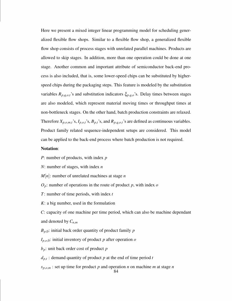
Here we present a mixed integer linear programming model for scheduling gener-

alized flexible flow shops. Similar to a flexible flow shop, a generalized flexible

flow shop consists of process stages with unrelated parallel machines. Products are

allowed to skip stages. In addition, more than one operation could be done at one

stage. Another common and important attribute of semiconductor back-end pro-

cess is also included, that is, some lower-speed chips can be substituted by higher-

speed chips during the packaging steps. This feature is modeled by the substitution

variables Rp,q,o,t’s and substitution indicators ξp,q,o’s. Delay times between stages

are also modeled, which represent material moving times or throughput times at

non-bottleneck stages. On the other hand, batch production constraints are relaxed.

Therefore Xp,o,m,t’s, Ip,o,t’s, Bp,t’s, and Rp,q,o,t’s are defined as continuous variables.

Product family related sequence-independent setups are considered. This model

can be applied to the back-end process where batch production is not required.

Notation:

P: number of products, with index p

N: number of stages, with index n

M[n]: number of unrelated machines at stage n

Op: number of operations in the route of product p, with index o

T : number of time periods, with index t

K: a big number, used in the formulation

C: capacity of one machine per time period, which can also be machine dependant

and denoted by Cn,m

Bp,0: initial back order quantity of product family p

Ip,o,0: initial inventory of product p after operation o

bp: unit back order cost of product p

dp,t : demand quantity of product p at the end of time period t

sp,o,m : set up time for product p and operation n on machine m at stage n84

tp,o,m : unit processing time of product p and operation o on machine m at stage n

cp,q,o : unit substitution cost for using product p as q at operation o

qp,n,m : product-machine qualification indicator, 1 if machine m at stage n is quali-

fied for product p and 0 otherwise

stage[o] : stage index for operation o

ξp,q,o: binary substitution indicator, 1 if product p can be used as product q at op-

eration o and 0 otherwise

delayp,o: delay time between operation o and the next operation in the route for

product p

Continuous Variables:

Xp,o,m,t : production quantity of product p and operation o in time period t on ma-

chine m at stage stage[o]

Ip,o,t : inventory quantity of product p at the end of time period t after operation o

Bp,t : back order quantity of the product p at the end of time period t

Rp,q,o,t : quantity of product q substituted by product p at operation o in time t

W 1p,o,m,t : time spent in time period t on the setup that ends in time period t for prod-

uct p and operation o on machine m at stage stage[o]

W 2p,o,m,t : time spent in time period t on the setup that continues in time period t +1

for product p and operation o on machine m at stage stage[o]

Lp,o,m,t : cumulative time by the end of time period t spent on the setup that con-

tinues to time period t + 1 for product p and operation o on machine m at stage

stage[o]

Binary Variables:

Yp,o,m,t : 1 if a setup for product p and operation o on machine m at stage stage[o]

ends in period t; 0 otherwise

Zp,o,m,t : 1 if product p and operation o can be processed on machine m at the be-

ginning of time period t +1 without a setup; 0 otherwise85

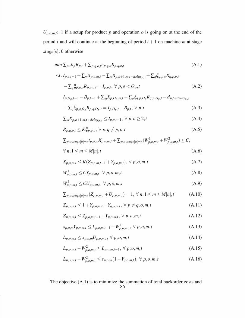
Up,o,m,t : 1 if a setup for product p and operation o is going on at the end of the

period t and will continue at the beginning of period t + 1 on machine m at stage

stage[o]; 0 otherwise

min ∑p,tbpBp,t +∑p,q,o,tcp,q,oRp,q,o,t (A.1)

s.t. Ip,o,t−1 +∑mXp,o,m,t −∑mXp,o+1,m,t+delayp,o +∑qξq,p,oRq,p,o,t

−∑qξp,q,oRp,q,o,t = Ip,o,t , ∀ p,o < Op, t (A.2)

Ip,Op,t−1 −Bp,t−1 +∑mXp,Op,m,t +∑qξq,p,OpRq,p,Op,t −dp,t+delayp,o

−∑qξp,q,OpRp,q,Op,t = Ip,Op,t −Bp,t , ∀ p, t (A.3)

∑mXp,o+1,m,t+delayp,o ≤ Ip,o,t−1, ∀ p,o ≥ 2, t (A.4)

Rp,q,o,t ≤ Kξp,q,o, ∀ p,q = p,o, t (A.5)

∑p,o:stage[o]=ntp,o,mXp,o,m,t +∑p,o:stage[o]=n(W1p,o,m,t +W 2

p,o,m,t)≤C,

∀ n,1 ≤ m ≤ M[n], t (A.6)

Xp,o,m,t ≤ K(Zp,o,m,t−1 +Yp,o,m,t), ∀ p,o,m, t (A.7)

W 1p,o,m,t ≤CYp,o,m,t , ∀ p,o,m, t (A.8)

W 2p,o,m,t ≤CUp,o,m,t , ∀ p,o,m, t (A.9)

∑p,o:stage[o]=n(Zp,o,m,t +Up,o,m,t) = 1, ∀ n,1 ≤ m ≤ M[n], t (A.10)

Zp,o,m,t ≤ 1+Yp,o,m,t −Yq,o,m,t , ∀ p = q,o,m, t (A.11)

Zp,o,m,t ≤ Zp,o,m,t−1 +Yp,o,m,t , ∀ p,o,m, t (A.12)

sp,o,mYp,o,m,t ≤ Lp,o,m,t−1 +W 1p,o,m,t , ∀ p,o,m, t (A.13)

Lp,o,m,t ≤ sp,o,mUp,o,m,t , ∀ p,o,m, t (A.14)

Lp,o,m,t −W 2p,o,m,t ≤ Lp,o,m,t−1, ∀ p,o,m, t (A.15)

Lp,o,m,t −W 2p,o,m,t ≤ sp,o,m(1−Yq,o,m,t), ∀ p,o,m, t (A.16)

The objective (A.1) is to minimize the summation of total backorder costs and86

total substitution costs. Constraints (A.2) are the inventory balance constraints for

each product at each operation except for the last in each time period. Each in-

ventory balance constraint states that the ending inventory quantity in period t is

equal to the starting inventory quantity plus production quantity minus consump-

tion quantity at next operation in the route of this product in a future period. Since

the delay time between the current operation o and the next operation in the route

is delayp,o, consumption quantity at the next operation in period t + delayp,o has

to be put into transit and thus removed from the inventory pile after operation o in

current period t. In addition, quantity of product p substituted by any other product

q and quantity of any other product q substituted by product p are also consid-

ered. Constraints (A.3) are the inventory balance constraints for each product at

last operation in each time period, and instead of the consumption quantity at the

next operation backorder quantity and demand quantity are considered. Constraints

(A.4) state that production quantity at operation o+1 in period t +delayp,o has to

be less than the available starting inventory at previous operation o in period t. Con-

straints (A.5) are the substitution constraints, indicating whether one product can

be substituted by another product. Constraints (A.6) are the capacity constraints

for each machine in each time period, stating that the total production and setup

times over all products and operations at one machine can not exceed the available

capacity of the machine in that time period. Constraints (A.7) state that processing

of product p for operation o can not be done on machine m unless the setup is car-

ried over from the previous time period (Zp,o,m,t−1 = 1) or finished in current time

period (Yp,o,m,t=1). Constraints (A.8) and Constraints (A.9) are constraints about

setup time decision variables W 1p,o,m,t and W 2

p,o,m,t based on their definitions. Con-

straints (A.10) state that at the end of any time period, the machine is either being

setup or producing. Constraints (A.11) states that if there is a setup completed for

product q in time period t and a setup status for product p is carried over to the next87

time period t +1, there has to be a setup completed for product p after product q is

processed in current time period t. Constraints (A.12) state that if a setup for prod-

uct p is carried over to the next time period t+1 (Zp,o,m,t = 1), there has to be either

a setup for product p completed in time period t (Yp,o,m,t = 1) or a setup for product

p carried over from previous time period t −1 (Zp,n,m,t−1 = 1). Constraints (A.13)

state that if a setup for product p and operation o on machine m is finished in period

t, the cumulative time spent on this setup, that is Lp,o,m,t−1 +W 1p,o,m,t , should be

greater than or equal to the required setup time sp,o,m. Constraints (A.14) are based

on the definition of Lp,o,m,t’s, stating that the cumulative setup time to be carried

over to the next period t, that is Lp,o,m,t , is set to zero unless the setup is continuing

in the next period t + 1. Constraints (A.15) and (A.16) together state that if there

is a setup completed for another product q in current time period t, the cumulative

setup time carried over to next time period for product t is set to W 2p,o,m,t ; otherwise,

the cumulative setup time carried over to next time period for product p is equal to

W 2p,o,m,t +Lp,o,m,t−1. Constraints (A.10-A.16) are used to model the condition when

one setup lasts over more than two time periods.

88

APPENDIX B

FUNCTIONS DEFINED IN SCHEDULER

The scheduler is based on a discrete event simulation structure, which means it

models every event and the status of every resource or constraint in the system. The

event types and functions defined in the scheduler are described in more details

here. There are six types of events defined in the scheduler: lot arrival to a stage

(arrival), lot departure from a machine (departure), end of a setup (end setup), end

of a preventive maintenance (end pm), end of a machine downtime (end down),

check and schedule of all idle machines at the beginning of every 2-hr time period

(check time point). When an event occurs, the status of a machine or a staff will

change. As a result, the system status will be updated according to the event type, as

shown in Algorithm 4. When a lot arrives at a stage, either machine from the stage

is chosen to process this lot or the lot is put in the queue, as shown in Algorithm 5.

In the scheduler, whenever before a idle qualified machine is setup for a product,

we will first check whether there is an available staff to perform the setup operation,

whether the number of machines already setup for the product at this stage is less

than the maximal number of machines allowed to be setup for this product at this

stage, as well as whether the setup and production of this lot will conflict any sched-

uled preventive maintenance or downtime of the machine. This check is performed

in line 3 of Algorithm 5. When a machine finishes processing a lot, Algorithm 6

is used to schedule an arrival event to the next operation and Algorithm 11 is then

called to choose a job/lot from the queue for the machine. When a setup, preventive

maintenance, or machine downtime ends, the status of a staff will change from busy

to idle, and thus Algorithm 11 is then called to choose a lot from the queue for the

machine, as shown in Algorithm 6, 8, 9, or 10. At the beginning of a 2-hr time

period, the status of all lots in the queue will change because we define the priority

of a lot by the product priority as well as comparison of the production time period

of the lot in the plan to current time period. If the production time period of a lot

in the plan is earlier than the current time period, the lot is defined as a late lot that90

has a higher priority. Otherwise the lot is defined as an early lot that has a lower

priority. So at the beginning of every 2-hr time period, Algorithm 11 will be called

to choose a lot from the queue for any idle machine at any stage.

Algorithm 4 main() Function1: while event list = empty ∥ current time = planning horizon do2: find next event with earliest event time in the event list3: if next event.type = arrival then4: run arrive()5: else if next event.type = departure then6: run depart()7: else if next event.type = check time point then8: run check time point()9: else if next event.type = end setup then

10: run end setup()11: else if next event.type = end pm then12: run end pm()13: else if next event.type = end down then14: run end down()15: end if16: end while

Algorithm 5 arrive() Function1: if there is at least one qualified idle machine then2: choose a machine with smallest setup time3: if a setup is needed for the chosen machine then4: if a setup can be performed for this product then5: change the status of the machine to being setup6: change the status of the worker to busy7: schedule an end setup event8: schedule a departure event9: else

10: put the job in the queue11: end if12: else13: change the status of the machine to being producing14: schedule a departure event from the machine15: end if16: else17: put the job in the queue18: end if

91

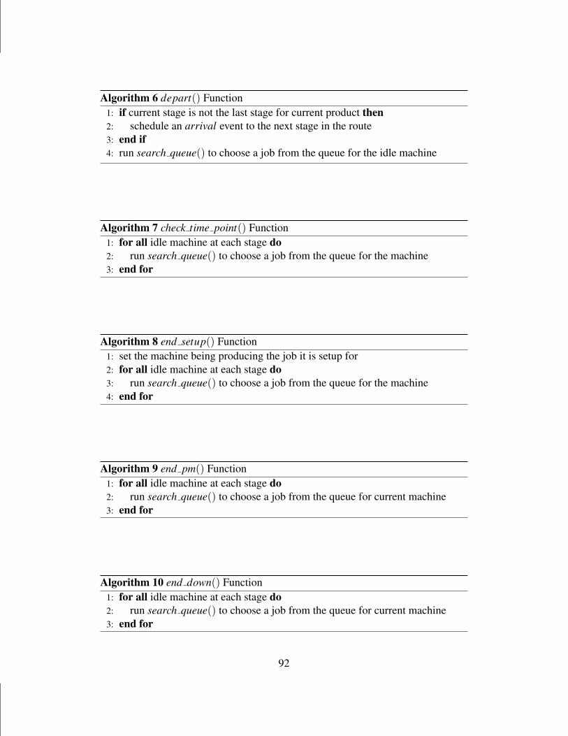
Algorithm 6 depart() Function1: if current stage is not the last stage for current product then2: schedule an arrival event to the next stage in the route3: end if4: run search queue() to choose a job from the queue for the idle machine

Algorithm 7 check time point() Function1: for all idle machine at each stage do2: run search queue() to choose a job from the queue for the machine3: end for

Algorithm 8 end setup() Function1: set the machine being producing the job it is setup for2: for all idle machine at each stage do3: run search queue() to choose a job from the queue for the machine4: end for

Algorithm 9 end pm() Function1: for all idle machine at each stage do2: run search queue() to choose a job from the queue for current machine3: end for

Algorithm 10 end down() Function1: for all idle machine at each stage do2: run search queue() to choose a job from the queue for current machine3: end for

92

Algorithm 11 search queue() Function1: search the queue in front of the stage for the best eligible job based on quali-

fication matrix, setup time length, product priority, and production time periodof the lot in the plan

2: if there is no eligible job then3: if there is a eligible job that can not be scheduled on the machine because of

conflicting a scheduled preventive maintenance/downtime then4: change the status of the machine from idle to preventive mainte-

nance/down5: schedule the pm/downtime end event6: else7: leave the machine idle8: end if9: else if the best eligible job is an early job then

10: if there is an eligible late job that can not be scheduled on the machine be-cause of conflicting a scheduled preventive maintenance then

11: change the status of the machine from idle to preventive maintenance12: schedule a pm end event13: else14: change the status of the machine from idle to be producing15: schedule a departure16: end if17: else if the best eligible job is an late job then18: schedule the late eligible job19: end if

93