PRODUCTION PLANNING AND SCHEDULING IN MULTI …home.iitk.ac.in/~pmehta/thesis.pdf · Production...
194
1 PRODUCTION PLANNING AND SCHEDULING IN MULTI-STAGE BATCH PRODUCTION ENVIRONMENT A THESIS SUBMITTED IN PARTIAL FULFILLMENT OF THE REQUIREMENTS FOR THE FELLOW PROGRAMME IN MANAGEMENT INDIAN INSTITUTE OF MANAGEMENT AHMEDABAD By PEEYUSH MEHTA Date: March 15, 2004 Thesis Advisory Committee __________________________[Chair] [PANKAJ CHANDRA] __________________________[Co-Chair] [DEVANATH TIRUPATI] __________________________[Member] [ARABINDA TRIPATHY]
Transcript of PRODUCTION PLANNING AND SCHEDULING IN MULTI …home.iitk.ac.in/~pmehta/thesis.pdf · Production...

1
PRODUCTION PLANNING AND SCHEDULING IN
MULTI-STAGE BATCH PRODUCTION ENVIRONMENT
A THESIS SUBMITTED IN PARTIAL FULFILLMENT OF THE REQUIREMENTS
FOR THE FELLOW PROGRAMME IN MANAGEMENT INDIAN INSTITUTE OF MANAGEMENT
AHMEDABAD
By
PEEYUSH MEHTA
Date: March 15, 2004
Thesis Advisory Committee
__________________________[Chair] [PANKAJ CHANDRA]
__________________________[Co-Chair] [DEVANATH TIRUPATI]
__________________________[Member] [ARABINDA TRIPATHY]

2
Production Planning and Scheduling in Multi-Stage Batch Production Environment
By Peeyush Mehta
ABSTRACT
We address the problem of jointly determining production planning and scheduling decisions in a complex multi-stage, multi-product, multi-machine, and batch-production environment. Large numbers of process and discrete parts manufacturing industries are characterized by increasing product variety, low product volumes, demand variability and reduced strategic planning cycle. Multi-stage batch-processing industries like chemicals, food, glass, pharmaceuticals, tire, etc. are some examples that face this environment. Lack of efficient production planning and scheduling decisions in this environment often results in high inventory costs and low capacity utilization.
In this research, we consider the production environment that produces intermediate
products, by-products and finished goods at a production stage. By-products are recycled to recover reusable raw materials. Inputs to a production stage are raw materials, intermediate products and reusable raw materials. Complexities in the production process arise due to the desired coordination of various production stages and the recycling process. We consider flexible production resources where equipments are shared amongst products. This often leads to conflict in the capacity requirements at an aggregate level and at the detailed scheduling level. The environment is characterized by dynamic and deterministic demands of finished goods over a finite planning horizon, high set-up times, transfer lot sizes and perishability of products. The decisions in the problem are to determine the production quantities and inventory levels of products, aggregate capacity of the resources required and to derive detailed schedules at minimum cost.
We determine production planning and scheduling decisions through a sequence of
mathematical models. First, we develop a mixed-integer programming (MIP) model to determine production quantities of products in each time period of the planning horizon. The objective of the model is to minimize inventory and set-up costs of intermediate products and finished goods, inventory costs of by-products and reusable raw materials, and cost of fresh raw materials. This model also determines the aggregate capacity of the resources required to implement the production plan. We develop a variant of the planning model for jointly planning sales and production. This model has additional market constraints of lower and upper bounds on the demand. Next, we develop an MIP scheduling model to execute the aggregate sales and productions plans obtained from the planning model. The scheduling model derives detailed equipment wise schedules of products. The objective of the scheduling model is to minimize earliness and tardiness (E/T) penalties.
We use branch and bound procedure to solve the production-planning problem. Demand of finished goods for each period over the planning horizon is an input to the model. The planning model is implemented on a rolling horizon basis.
3
We consider flowshop setting for the finished goods in the production environment. The due dates of finished goods are based on the customer orders. We report some new results for scheduling decisions in a permutation flowshop with E/T penalties about a common due date. This class of problems can be sub-divided into three groups- one, where the common due date is such that all jobs are necessarily tardy; the second, where the due date is such that the problem is unrestricted; and third is a group of problems where the due date is between the above two. We develop analytical results and heuristics for flow shop E/T problems arising in each of these three classes. We also report computational performance on these heuristics. The intermediate products follow a general job shop production process with re-entrant flows. We develop heuristics to determine equipment wise schedule of intermediate products at each level of the product structure. The due date of an intermediate product is based on the schedule of its higher-level product.
The models developed are tested on data for a chemical company in India. The results
of cost minimization model in a particular instance indicated savings of 61.20 percent in inventory costs of intermediate products, 38.46 percent in set-up costs, 8.58 percent in inventory costs of by-products and reusable raw materials, and 20.50 percent in fresh raw material costs over the actual production plan followed by the company. The results of the contribution maximization model indicate 42.54 percent increase in contribution. We also perform sensitivity analysis on results of the production planning and scheduling problem.
The contribution of this research is the new complexities addressed in the production
planning and scheduling problem. Traditional models on multi-stage production planning and scheduling are primarily based on assembly and fabrication types of product structures and do not consider the issues involved in recycling process. Scheduling theory with E/T penalties is largely limited to single machine environment. We expect that models developed in this research would form basis for production planning and scheduling decisions in multi-stage, multi-machine batch processing systems. The sensitivity analysis of the models would provide an opportunity to the managers to evaluate the alternate production plans and to respond to the problem complexities in a better way.

4
Acknowledgements
I wish to express my deepest gratitude to my thesis advisor Professor Pankaj Chandra.
He has been a tremendous source of learning for me during my stay at IIMA. Professor
Chandra has been a great motivator, and has a significant share in my academic grooming.
Much of the credit for this work goes to Professor Devanath Tirupati, co-chair of my thesis
committee. He has been very patient with me and has provided very useful research training. I
would also like to thank Professor Arabinda Tripathy, member of my thesis committee for
providing very useful feedback throughout my work.
I am grateful to Professor Diptesh Ghosh, Professor P. R. Shukla, Professor Ashok
Srinivasan and Professor Goutam Dutta for their useful feedback on my thesis. I am also
thankful to Professor Shiv Srinivasan for giving some pointers on the drafting of this
document.
I wish to especially thank my wife Ritu, as this thesis would not have been possible
without her support. She has a major share in raising our daughter Riti, and her break from her
professional career helped me to stay focused on my work Riti always provided the much-
needed break from the thesis work. I dedicate this work to my parents. They have eagerly
waited to see me accomplish this work. Dhiraj, my brother, has been, as always, a source of
encouragement.
I would like to thank my colleagues Bharat, Rohit, Satyendra and all those with whom
I have interacted at various stages of my thesis. The staff members of FPM office, computer
center and library have obliged me in more ways than one.

5
Table of Contents 1 Introduction................................................................................................................. 9
1.1 Introduction................................................................................................................... 9
1.2 Production Planning and Scheduling Problem ........................................................... 12 1.2.1 Production Environment .............................................................................................13
1.2.2 Complexities in the Production Environment ................................................................16
1.2.3 Production Planning and Scheduling Decisions.............................................................18
1.3 Summary..................................................................................................................... 19 2 Literature Review ..................................................................................................... 21
2.1 Integrated Production Planning and Scheduling Models ............................................ 22
2.2 Hierarchical Production Planning and Scheduling Models ........................................ 29
2.3 Earliness and Tardiness Scheduling............................................................................ 34
2.4 Research Gaps............................................................................................................. 42 3 Production Planning and Scheduling Models ........................................................ 44
3.1 Introduction................................................................................................................. 44
3.2 Production Planning Model ........................................................................................ 46 3.2.1 Formulation of Production Planning Model...................................................................46
3.3 Scheduling Models...................................................................................................... 51 3.3.1 Finished Goods Scheduling Problem Formulation.........................................................52
3.3.2 Intermediate Products Scheduling Problem Formulation................................................54
3.4 Summary..................................................................................................................... 56 4 Solution Procedure for Production Planning and Scheduling Problem.............. 57
4.1 Introduction................................................................................................................. 57
4.2 Solution Procedure for Production Planning and Scheduling Problem...................... 58
4.3 Solution Procedure for Production Planning Problem................................................ 58
4.4 Solution Procedure for Finished Goods Scheduling Problem................................... 60
4.4.1 Sub-Problem 1: Flowshop E/T Problem for Unrestricted Common Due Date..................65
4.4.2 Sub-Problem 2:Flowshop E/T Problem for Intermediate Common Due Date ..................67 4.4.3 Sub-Problem 3:Flowshop Tardiness Problem for Common Due Date.............................75
4.5 Solution Procedure for Intermediate Products Scheduling Model ............................. 79
4.6 Dedicated Plant Scheduling Heuristic ........................................................................ 87

6
4.7 Summary..................................................................................................................... 92 5 Results of Production Planning and Scheduling Problem .................................... 93
5.1 Introduction................................................................................................................. 93
5.2 Results of Sub Problem 2............................................................................................ 94 5.2.1 Lower Bound of Sub Problem 2...................................................................................94
5.2.2 Experiment Design of Sub Problem 2...........................................................................95
5.3 Results of Sub Problem 3.......................................................................................... 101 5.3.1 Lower Bound of Sub Problem 3 (Ahmadi and Bagchi, 1990) ....................................... 102
5.3.2 Existing Results of Sub Problem 3............................................................................. 104
5.4 Production Planning and Scheduling Results ........................................................... 110
5.5 Summary................................................................................................................... 111 6 Case Study: Application of Production Planning and Scheduling Models ....... 114
6.1 Introduction............................................................................................................... 114
6.2 Production Planning and Scheduling Problem ......................................................... 115
6.3 Application of Production Planning Model .............................................................. 117
6.3.1 Results of Production Planning Model....................................................................... 118
6.4 Contribution Maximization Model ........................................................................... 120
6.5 Application of Scheduling Model............................................................................. 124
6.6 Sensitivity Analysis on Production Planning and Scheduling Results ..................... 125
6.7 Implementation Issues............................................................................................... 128
6.8 Summary................................................................................................................... 129 7 Summary, Contribution and Future Research .................................................... 134
7.1 Summary................................................................................................................... 134
7.2 Contribution.............................................................................................................. 139
7.3 Future Research......................................................................................................... 141 References............................................................................................................................ 144
Appendices........................................................................................................................... 154
Appendix 1: Product Structure Diagrams and Process Flow Diagrams ............................... 154
Appendix 2: Base Case Production Plan and Schedule ........................................................ 164
Appendix 3: Sensitivity Analysis on Production Planning and Scheduling Results ............ 180

7
List of Figures
Figure 1.1: Multi- level Product Structure and Concept of Stage ............................................ 13
Figure 1.2: Machines, Operations and Routes of a Product ................................................... 14
Figure 1.3: Inputs and Outputs of a Production Process......................................................... 15
Figure 4.1: Schematic of Solution Procedure for Production Planning and Scheduling
Problem................................................................................................................. 59
Figure 4.2: Flowshop E/T Problem Decomposition Based on Due Dates.............................. 64
Figure 4.2: Conflict Removal at a Machine ............................................................................ 80
Figure 5.1: Average % Deviation of Heuristic Solution from Lower Bound: 5 Machines .... 97
Figure 5.2: Average of Deviation of Heuristic Solution from Lower Bound: 10 Machines .. 98
Figure 5.3: Average % Deviation from Optimal Solution and its Square Root ..................... 99
Figure 5.4: Improvement in the solution with Increase in Number of Tabu Iterations ........ 100
Figure 5.5: Comparison of Results with Different Tabu Iterations ...................................... 101
Figure 5.6: Average % Deviation of Heuristic Solution from Lower Bound: 5 Machines, Sub-
Problem 3 ............................................................................................................ 106
Figure 5.7: Average % Deviation of Heuristic Solution from Lower Bound: 10 Machines,
Sub-Problem 3..................................................................................................... 107
Figure 5.8: Average % Deviation of Heuristic Solution from Lower Bound: 15 Machines,
Sub-Problem 3..................................................................................................... 108
Figure 5.9: Average % Deviation of Heuristic Solution from Lower Bound: 20 Machines,
Sub-Problem 3..................................................................................................... 109
Figure 6.1: Multi-Level Product Structure............................................................................ 115

8
List of Tables
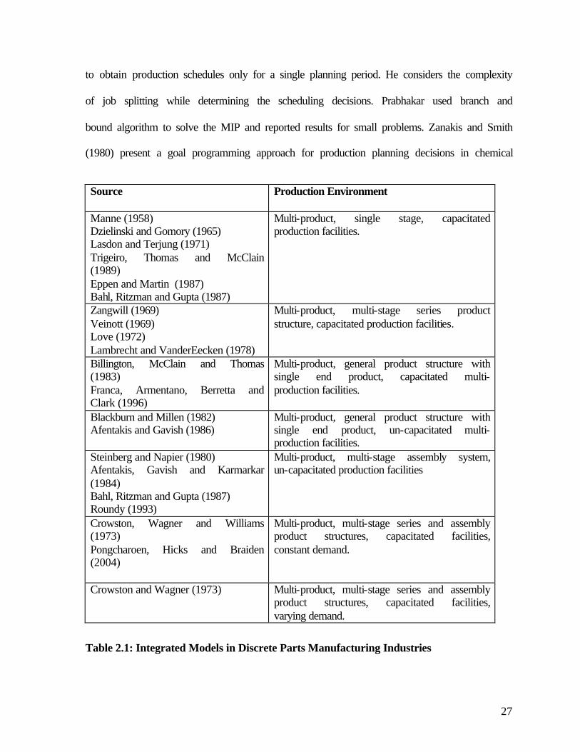
Table 2.1: Integrated Models in Discrete Parts Manufacturing Industries ............................. 27
Table 2.2: Integrated Models in Process Industries. ............................................................... 29
Table 2.3: Hierarchical Models in Discrete Parts Manufacturing Industries.......................... 32
Table 2.4: Hierarchical Models in Process Industries ............................................................ 33
Table 2.5: Single Machine Schedule with Earliness and Tardiness Penalties ........................ 40
Table 5.1: Parameters in Experiment Design of Sub-Problem 2 ............................................ 95
Table 5.2: Average Percentage of Deviation of Optimal Solution from Heuristic Solution.. 99
Table 5.3: Production Plan of Finished Goods ..................................................................... 111
Table 6.1: Comparison of Model Results with Actual Production Plan Costs ..................... 120
Table 6.2: Percentage Increase in ‘Revenue Net of Material Cost’ in Contribution
Maximization Model as Compared to the Actual Sales and Production Plan. ... 122
Table 6.3: Production Costs Difference In Percentage: (Actual Production Plan–Production
Plan Proposed by the Model) .............................................................................. 122
Table 6.4: Sensitivity Analysis on Production Planning and Scheduling Results ................ 130
Table 6.5: Capacity Utilization (in Percentage) of Dedicated Plants ................................... 131
Table 6.6: Capacity Utilization (in Percentage) of Machines in Flexible Plants .................. 132

9
1 Introduction
1.1 Introduction
Today’s business environment has become highly competitive. Manufacturing firms
have started recognizing the importance of manufacturing strategy in their businesses. Firms
are increasingly facing external pressures to improve customer response time, increase
product offerings, manage demand variability and be price competitive. In order to meet
these challenges, firms often find themselves in situations with critical shortages of some
products and excess inventories of other products. This raises the issue of finding the right
balance between cutting costs and maintaining customer responsiveness. Firms are facing
internal pressures to increase profitability through improvements in manufacturing efficiency
and reductions in operational costs.
There are several instances in industry where the above-mentioned changes in
business environment have affected the profitability of firms. Harris Corporation, an
electronics company based in U.S.A., increased its product range considerably and invested
in flexible manufacturing resources in the early 1990s. They had to provide competitive on-
time delivery performance over a much greater product mix. Their inefficient handling of a
large product variety resulted in late deliveries, lost sales and average losses of $75 million
annually (Leachman et al., 1996). IBM faced record losses in 1993 in the manufacturing and
distribution operations of its computer business due to high operational costs. They could not
handle the high demand variability of their products and reported high inventory costs and
stock outs (Feigin et al., 1996). Fuel inventory costs have risen considerably in electric utility
industries in U.S.A. in the last two decades as a result of electricity demand fluctuations

10
(Chao et al., 1989). H&R Johnson, the largest tile manufacturer in India, had to increase its
product variety in terms of size and design, in order to meet the demand of expanding
construction market. This resulted in high inventory costs. Their customer response time
increased considerably, resulting in loss of sales (Gupta, 1993). Synpack, an Indian chemical
manufacturing firm, increased its product portfolio in the mid 1990s. However, it could not
handle the delivery commitments. The company’s market share reduced considerably and
they incurred high inventory costs (Akthar, 2004).
Indian manufacturing firms are facing stiff global competition, especially from China.
Today, China has become the world’s largest manufacturing base. China’s capability to offer
a large variety of products at low prices, and its fast responsiveness to the market has
severely affected the sales of many Indian manufacturing firms. Indian companies are now
forced to be competitive on prices, increase product offerings, and have shorter lead times in
production.
The implications of the above–mentioned challenges in the business environment are
that manufacturing firms are now forced to focus on cost-leadership issues, optimize the use
of available resources, and reduce their operational costs. They have to constantly explore
manufacturing strategies to meet these objectives.
Since the mid 1980s, the business press has highlighted the success of many
Japanese, European, and North American firms in achieving a high degree of efficiency in
manufacturing (Silver et al., 1998). In recent years, many of these firms have started to
coordinate with other firms in their supply chain. For example, instead of responding to
demand variability, firms share information with their partners to analyze demand pattern. It

11
is observed that this notion, although useful, is not a sufficient way of facing some of the
challenges discussed earlier. Most managers assume that new levels of efficiency can be
obtained simply by sharing information and forming alliances with their partners. They do
not realize that information and data have to be used with very clear objectives. Here, the role
of inventory management and production planning and scheduling is introduced. Developing
sound production planning and scheduling strategies may seem mundane in comparison to
strategy formulation, but it is observed that these strategies are critical to long-term survival
and competitive advantage.
Production planning and scheduling help considerably in reducing operational costs,
improving customer service and utilizing the resources optimally. In the examples discussed
above of high operational costs incurred by firms, significant savings have been realized
using production planning and scheduling. By applying optimization based production-
planning system, Harris Corporation raised its on-time deliveries from 75 to 95 percent
without increasing inventories and converted its huge losses to an annual profit $40 million.
Over the past two decades, IBM's operations research team developed production-planning
systems and helped save hundreds of millions of dollars, while improving operations and
competitive strategies. H&R Johnson implemented production-planning tools and reduced its
production lead times and inventory costs.
Production planning and scheduling find their applicability in both discrete parts
manufacturing and process industries. APICS1 dictionary provides the key elements to
classify industries as process or discrete parts (Blomer and Gunther, 1998; Crama et al.,
2001). More and more process industries are shifting to specialties market with customized 1 American Production and Inventory Control Society

12
products and are no longer operating on make-to-stock policy alone. This is especially true of
batch process industries such as pharmaceuticals, food, and glass, etc. These industries do not
restrict themselves to commodity products only. The first significant applications of
production planning and scheduling methods in process industries were in oil refineries, food
processing and steel manufacturing. Through the years, production planning and scheduling
methods have been developed and applied to process manufacturing of other products such
as chemicals, paper, soap and industrial gases.
The main motivation for this research is to observe the potential benefits of
production planning and scheduling in manufacturing industries. The aim is to investigate the
benefits of production planning and scheduling in complex production environments.
The remainder of this chapter is organized as follows. In the next section, we discuss
the production planning and scheduling problem addressed in this research. We begin by
describing the production environment in sub section 1.2.1. In sub-section 1.2.2, we discuss
the complexities in the production environment. We describe the decisions to be addressed in
the production planning and scheduling problem in sub-section 1.2.3. The summary of this
chapter is provided in section 1.3.
1.2 Production Planning and Scheduling Problem
In this section, we describe the production planning and scheduling problem
addressed in this research. First we describe the production environment. The motivation for
the production environment considered in this research is largely from our observations on
characteristics of chemical plants. Then we describe the complexities in the production

13
environment. Subsequently we focus on the decisions to be addressed in the production
planning and scheduling problem.
1.2.1 Production Environment
We consider multi-stage production environment that produces both intermediate
products and finished goods. A stage in the production environment corresponds to the
production of an intermediate product or a finished good. The concept of multi-stage in the
environment considered is equivalent to the multi-level product structure, as shown below for
illustration in figure 1.1. In figure 1.1, level 0 products are finished goods (E1, E2, E3), level
1 and level 2 products are intermediate products (I1,I2,…I6). The levels in the product
structure diagram are various stages of the production process. For instance, level 1 and level
2 in figure 1.1 are the intermediate products stages. The intermediate products at level 2 are
inputs to the intermediate products at level 1. Level 1 intermediate products are inputs to
level 0 products, which are finished goods, and at the finished goods production stage.
Figure 1.1: Multi-level Product Structure and Concept of Stage
The production environment has multiple production plants to produce intermediate
products and finished goods. A production plant consists of number of equipment, called as
E1 E2 E3
I1 I2 I3
I4 I5 I6
Level 0
Level 1
Level 2

14
‘machines’. Intermediate products and finished goods are processed on machines in a
production plant in a specific order. The processing of a product on a machine is called an
‘operation’. A ‘route’ is defined as the sequence of machines used for processing a product.
To illustrate these concepts, we use figure 1.2 below. Consider a product ‘P’, it requires four
operations in a production plant. There are five machines in the plant in this example
(M1,M2,..,M5). As indicated in figure 1.2, there is choice of machines between M3 and M4
for third operation. That is, based on the machine used for third operation of product P, there
are two different routes, Route 1 and Route 2 to produce product P. Route 1 comprises
machines M1, M2, M3, M5 and Route 2 comprises machines M1, M2, M4 and M5.
Figure 1.2: Machines, Operations and Routes of a Product
There are two types of production plants in the production process. One is the
dedicated production plant. In the dedicated production plant, only one type of product is
produced. The second type is the flexible plant. In the flexible production plant, intermediate
products and finished goods share machines.
A by-product is generated, when an intermediate product or a finished good is
produced in a production plant. A by-product consists of reusable raw materials. By-
Route 1 Route 2
M1 M2
M3
M4
M5
Operation 1 Operation 2 Operation 3 Operation 4

15
products are processed in a separate recycling plant, and some reusable raw materials are
recovered from the recycling process. Part of the raw materials that is not recovered for reuse
becomes waste. Figure 1.3 shows the inputs and outputs of the production process and
linkages between the production plants and the recycling plants.
Figure 1.3: Inputs and Outputs of a Production Process
It can be seen in figure 1.3 that inputs to production process in a plant are the fresh
raw materials, reusable raw materials and intermediate products. The outputs of a production
process from a plant are intermediate products, finished goods and by-products. By-products
are processed in recycling plants to recover reusable raw materials. Reusable raw materials
are used again as inputs in the production process.
We consider flowshop setting for the finished goods in the production environment.
In a flowshop, all products follow a similar route in a production plant. Intermediate products
follow a general job shop setting with re-entrant flows. In a general job shop, the routes of
products are distinct. The characteristic of a re-entrant job shop is that jobs are processed on
a particular machine for more than one operation.
Recycling Plant
Reusable Raw Materials
Intermediate Products Plant
Fresh Raw Materials Intermediates
By Products Intermediates
Finished Goods Plant
Fresh Raw Materials
By Products Finished Goods
Waste

16
1.2.2 Complexities in the Production Environment
In this sub-section, we describe some of the complexities that exist in the production
environment. The production environment discussed in previous sub-section, and the
complexities in the production environment, form the basis for production planning and
scheduling decisions.
As seen in figure 1.3, raw materials are recovered from by-products through a
recycling process and reused in the production process. The recycling process is an important
tool in reducing the operational costs, as the cost of raw materials is very high. Maximum
recovery of the raw materials would translate to less use of fresh raw materials in the
production process. It is desirable to run the recycling plants when the production plants are
in operation. The reason for this argument is that by-products and reusable raw materials
have limited storage capacity. Simultaneous generation and recycling of by-products would
minimize the storage of by-products and recovered raw materials. This also translates into
maintaining lesser inventory of fresh raw materials, because more reusable raw materials are
being used in the production process. The above discussion leads to requirement of
coordinating the production process and the recycling process. The production plans of the
plants should be synchronized with the recycling plants to reduce the operational costs.
In a multi-stage environment, inventory is in the form of intermediate products and
finished goods. To minimize production costs, inventory of the products needs to be
minimized. This objective results in complexity of coordinating the schedules of products
across the production plants. If production plants were decoupled with each other while
scheduling, considerably high amount of inventory would be required to avoid production

17
delays. When an intermediate product or an end product is scheduled, intermediate products
that are inputs to the product should be available. Inventory of products will be reduced if the
production plants are synchronized, i.e., when an intermediate product is produced, its
higher-level product (where it is an input) is ready for processing. Similarly, the availability
of raw materials with their minimum inventory is to be ensured before scheduling products.
There are high setup times in the production process. During product changeover at a
flexible machine, idle time is incurred. In chemical plants, because of the chemical properties
of products, residues have to be removed thoroughly at each changeover, and this results in
considerable amount of idle time. There are trade-offs between setup costs and inventory
costs. Higher production run of a product in a setup would result in high inventory cost,
whereas more number of setups would consume significant amount of capacity in setups.
Intermediate products and finished goods are perishable. They have to be consumed
within a specific time period, else they become waste. To minimize wastage and to avoid any
production delays resulting from wastage, production plans at the plants need to be
synchronized based on the shelf life of products.
Intermediate products are transferred to another production plant or within the same
production plant, for next stage production, through transfer lot size of products. Only after
certain quantity specified by the transfer lot size is produced, the product is transferred for its
consumption. This again leads to the requirement of coordinating the production plants on
the basis of transfer lot sizes.
There is also a trade-off between purchasing the intermediate products and their in-
house production. The implications of purchasing the intermediate products are twofold.
18
Purchasing would obviously result in higher production costs, but this also can help in
minimizing production delays.
Demand variability adds to the complexity in the system. The production planning is
done on the basis of combination of firm orders and demand forecast over a finite planning
horizon. The implication of demand variability is that if the demand forecast is not correct,
there would be high inventory levels of some products and stock outs of other products.
Another implication of demand fluctuation is that within the planning period, frequent
revision in production plan and schedule is required to absorb the variation in demand.
Based on the production environment and its complexities discussed above, we
describe in the next sub-section, the production planning and scheduling problem. We also
formalize the decisions to be addressed in the production planning and scheduling problem.
1.2.3 Production Planning and Scheduling Decisions
In this sub-section, we characterize the production planning and scheduling problem
based on the decisions to be addressed in the problem. There are two sets of decisions in the
problem. One set of decisions is the production planning decisions. The other set is the
scheduling decisions.
Production planning decisions are aggregate decisions and tactical in nature. One of
the production planning decisions is to determine the production quantity of intermediate
products and finished goods in each time period of the planning horizon. Production planning
also determines the aggregate capacity of resources required to meet the production plan in
each time period is to be determined. The production planning costs are the inventory costs
19
of products and setup costs incurred over the planning horizon. The production-planning
problem is to determine the decisions discussed above at minimum cost.
Scheduling decisions are more detailed and operational in nature. The time horizon of
scheduling decisions is relatively short. For each product, the start time and the completion
time on each machine is to be determined. The scheduling costs consists of inventory costs
and costs incurred due to delay in satisfying customer orders. The formal definition of
scheduling costs is provided later in chapter 3. The scheduling problem in our research is to
determine the scheduling decisions at minimum cost. We are dealing with deterministic
scheduling, i.e., at the time of scheduling, all the information that defines a problem instance
is known with certainty. The information lending the scheduling problem to be deterministic,
for example, is the known processing time of products, and machine availability.
1.3 Summary
In this chapter, we have discussed some of the changes occurring in the business
environment as a result of increasing global competitiveness of firms. We highlighted the
increasing importance of reducing operational costs of firms in the changing environment. It
was discussed that production planning and scheduling is one of the important tools in
reducing the operational costs of firms. We provided a detailed description of production
planning and scheduling problem addressed in this research. Then, we discussed the
production environment in detail along with the complexities of the production environment.
We also focused on the decisions to be addressed in the production planning and scheduling
problem.

20
The rest of the thesis is organized as follows. In the next chapter, we provide the
literature review of the production planning and scheduling problem considered in this
research. Chapter 3 describes the mathematical models for addressing the production
planning and scheduling decisions. In chapter 4, we discuss the solution algorithms for
solving the production planning and scheduling problem. In chapter 5, we report the results
of the solution algorithms used to solve production planning and scheduling problem. We
also provide sensitivity analysis on results of the production planning and scheduling
problem in this chapter. In chapter 6, we apply the production planning and scheduling
models to a real life problem of pharmaceutical company in India. The results of this
application and the sensitivity analysis on the results are provided in this chapter. In chapter
7, we provide the summary of this research, contribution from this research, and discuss
some issues relating to future research.

21
2 Literature Review
In this chapter, we review the research on production planning and scheduling
problems in discrete parts manufacturing and process industries. There has been a renewed
interest in application of mathematical programming to address production planning and
scheduling decisions (Graves et al., 1993). The interest is mainly due to recent advances in
information technology as it allows production managers to acquire and process production
data on a real-time basis. As a result, managers are actively seeking decisions support
systems to improve their decision-making. We will review some of the mathematical
programming models developed and applied to the industry problems.
Primarily, there exist two types of approaches to address the production planning and
scheduling decisions. One is the integrated approach, where production planning and
scheduling decisions are determined simultaneously in a single monolithic model. The other
approach is the hierarchical approach, where production planning and scheduling decisions
are determined sequentially through separate models at an increasing level of detail. Both the
approaches have been applied to solve the production planning and scheduling problems. We
will study the mathematical models in both the approaches in this chapter.
Most of the research in scheduling theory with consideration of due dates has focused
on minimizing the delay in customer orders (tardiness). The formal definition of tardiness is
provided later in the chapter. Recently, the scheduling researchers have started investigating
issues related to earliness of a job. Just-in-Time (JIT) philosophy has been the main driving
force for this interest. We will study several other reasons for considering earliness as one of
scheduling objectives later in the chapter.

22
The plan of this chapter is as follows. In the next section, we discuss the integrated
mathematical models developed in discrete parts manufacturing and process industries. In
section 2.2, we review hierarchical production planning and scheduling models. Section 2.3
describes the work done in scheduling with earliness and tardiness penalties. In section 2.4,
we identify certain research gaps from this literature review.
2.1 Integrated Production Planning and Scheduling Models
We begin by reviewing the integrated models applied to single-stage and multi-stage
production environment in discrete parts manufacturing industries. Then we will consider the
models in process industries. Manne (1958) was the first to propose a production-scheduling
model for multi–product, single-stage, and batch processing environment. Manne developed
a linear program that provided a good approximation when the number of products being
manufactured is large in comparison to the number of time periods. The solution procedure
developed by Manne does not provide optimal solution to the problem. Dzielinski and
Gomory (1965) further developed the model suggested by Manne (1958) by applying
Dantzig-Wolfe decomposition to the problem. Application of the decomposition principle
yields an equivalent linear program, called the master program, with fewer constraints and
variables. The decomposition methods in the solution procedure provided by Dzielinski and
Gomory helped in reducing the computations, but the solution obtained is far from optimal.
The linear program being decomposed is only an approximation to an integer program whose
solution is actually desired. Lasdon and Terjung (1971) applied the column generation
procedure to the multi-product, single-stage integrated production-scheduling problem. They
do not consider the master problem as done by Dzielinski and Gomory. Instead, the large

23
number of variables is handled by column generation via sub-problems. They derive a lower
bound of the problem and use it as the termination criterion for computations. The solution
procedure from Lasdon and Terjung requires half the number of iterations as compared to the
work of Dzielinski and Gomory. However, the solution obtained by Larson and Terjung also
is quite far from the optimal solution. In fact, the solutions suggested by Manne (1958),
Dzielinski and Gomory (1965) and Lasdon and Terjung (1971) are not necessarily feasible
and the reported costs are not necessarily correct. This is because setup times and costs are
charged only once even when a batch is split between periods. The authors have
approximated these costs with the reason that with many products produced in each period,
the percentage of unaccounted setups is usually small. Thus, in all three papers, the costs are
underestimated and the capacity is not sufficient to allow for setups in some periods. This
will sometimes result in infeasible schedules. Eppen and Martin (1987) developed tighter
linear programming and lagrangian relaxation for multi-product, single stage production
scheduling problems. They show that the linear programming relaxation generates bounds
equal to those generated using lagrangian relaxation or column generation. Eppen and Martin
report on successful experiments with models consisting of upto 200 products and 10 time
periods. Trigeiro, Thomas and McClain (1989) reported on computational experience using
lagrangian relaxation on large multi-product, single-stage models with high setup times.
They improved on the weakness of underestimating set-up times and set-up costs in above
mentioned three papers. However, the solution procedure provided by Trigeiro, Thomas and
McClain also does not guarantee feasibility of scheduling decisions.
Multi-stage production environment introduces dependent demand of products.
Production quantities and schedules of products at a particular level depend on the decisions

24
made for the products at higher levels (parents or successors). Earlier work in multi-stage
batch processing system is by Zangwill (1969) and Veinott (1969). They presented efficient
solution techniques with dynamic programming for un-capacitated serial product structure.
The computational requirements increase considerably with problem size in the solution
procedures of Zangwill and Veinott. Love (1972) shows that if production costs are non-
decreasing from intermediate products stage to end products stage, then an optimal schedule
has the property that if in a given period, stage j produces, then stage j + 1 also produces.
This nested structure is exploited by Love in an algorithm for finding an optimal schedule.
Crowston, Wagner and Williams (1973) analyzed multi-machine lot sizing decisions by
constructing dynamic programming algorithm in serial and assembly product structures, with
constant demand in an infinite planning horizon. However, they consider only one
component at a level, and the solution procedure is characterized by excessive computational
requirements. Crowston and Wagner (1973) extended the results of Love (1972) to present
dynamic programming algorithm for assembly structures with known but varying demand
over the finite-planning horizon. The solution time of the algorithm increases exponentially
with the number of time periods, but only linearly with the increase in number of stages.
Crowston and Wagner also apply branch and bound algorithm for large number of time
periods but with serial product structures only. Lambrecht and VanderEecken (1978) present
a heuristic approach for serial product structure with only one capacity constraint. Blackburn
and Millen (1982) consider serial and assembly product structures with un-capacitated
production facility. Through series of simulation experiments, Blackburn and Miller report
potential errors in single- pass, stage-by-stage heuristic approaches for lot-sizing decisions in
multi-stage systems. One major weakness in all the research discussed so far on multi-stage

25
environment is that they do not consider component commonality, i.e., a product with more
than one successor or parent. This assumption is unrealistic for many plant environments.
Steinberg and Napier (1980) were the first to consider product commonality by proposing a
formulation that is a constrained generalized network framework. This work brings out the
importance of commonality and serves as a benchmark for evaluating heuristic algorithms.
However, the model is solved with a mixed integer programming code, which limits its
application to small problems. Billington, McClain and Thomas (1983) formulate a mixed-
integer program to model the capacity constrained multi-stage general product structure
production-scheduling problem for determining lot–sizing decisions, production lead-times
and capacity planning. They allow product commonality in the product structure, a feature
largely ignored in the previous work. Billington, McClain and Thomas develop heuristic
procedures to reduce the problem size on the basis on number of common products. Their
solution procedure is not useful for large problems and the heuristic solution is found to be
very far from the optimal solution. Afentakis, Gavish and Karmarkar (1984) developed
algorithms to obtain optimal solutions for single-product assembly product structures for un-
capacitated systems. They decompose the problem into set of single stage production
planning problems linked by a set of dual prices. They solve these single stage problems
using a fast shortest path algorithm. This natural decomposition has been used as an efficient
way to develop lower bounds to the optimal solution. They incorporate the lower bounds in a
branch and bound procedure and solve problems up to 50 products in 15 stages for 18 periods
in the planning horizon. However, their solution is for assembly product structures only.
Aftentakis and Gavish (1986) relax this restriction and examine the lot-sizing problem in the
general product structure systems with un-capacitated production facilities. The solution

26
procedure for the problem defined with general product structure is more complex than the
one defined on assembly systems. Afentakis and Gavish transform the general product
structure problem into an equivalent and larger assembly system. They apply lagrangian
relaxation that yields easily solvable sub-problems. However, this approach significantly
increases the number of variables. They report computational results with only 3 end
products and 15 stages over a 12 period planning horizon. Franca, Armentano, Berretta and
Clark (1996) consider the lot sizing decisions in multi-stage capacitated systems with
assembly and general product structures. They develop heuristic algorithms that perform well
only with large capacity, fewer setups, and assembly product structures. They report
computational results upto 17 products and 10 time periods. Pongcharoen, Hicks and Braiden
(2004) consider multi-stage, capacitated production planning and scheduling problem in
assembly product structures. They use genetic algorithms based heuristics but report results
for small problems only. Bahl, Ritzman and Gupta (1987) and Karimi, Ghomi and Wilson
(2003) provide a review of the production planning models for discrete parts manufacturing
applications. Table 2.1 summarizes the models developed in single and multi-stage batch
processing systems for discrete parts manufacturing environment.
Mathematical programming applications for production-planning decisions have been
used in process industries like oil, steel, petroleum, food etc. Eilon (1969) proposed a mixed
integer program (MIP) for production scheduling in multi-product, single stage environment
with capacity constraints in a chemical industry. He developed heuristic algorithms based on
batch scheduling approach to schedule 5 products, subject to normal demand distribution
with known parameters. In a two-stage production environment, Prabhakar (1974) studied lot
sizing and sequence dependent setup time sequencing in the chemical industry using an MIP
27
to obtain production schedules only for a single planning period. He considers the complexity
of job splitting while determining the scheduling decisions. Prabhakar used branch and
bound algorithm to solve the MIP and reported results for small problems. Zanakis and Smith
(1980) present a goal programming approach for production planning decisions in chemical
Source Production Environment
Manne (1958) Dzielinski and Gomory (1965) Lasdon and Terjung (1971) Trigeiro, Thomas and McClain (1989) Eppen and Martin (1987) Bahl, Ritzman and Gupta (1987)
Multi-product, single stage, capacitated production facilities.
Zangwill (1969) Veinott (1969) Love (1972) Lambrecht and VanderEecken (1978)
Multi-product, multi-stage series product structure, capacitated production facilities.
Billington, McClain and Thomas (1983) Franca, Armentano, Berretta and Clark (1996)
Multi-product, general product structure with single end product, capacitated multi-production facilities.
Blackburn and Millen (1982) Afentakis and Gavish (1986)
Multi-product, general product structure with single end product, un-capacitated multi-production facilities.
Steinberg and Napier (1980) Afentakis, Gavish and Karmarkar (1984) Bahl, Ritzman and Gupta (1987) Roundy (1993)
Multi-product, multi-stage assembly system, un-capacitated production facilities
Crowston, Wagner and Williams (1973) Pongcharoen, Hicks and Braiden (2004)
Multi-product, multi-stage series and assembly product structures, capacitated facilities, constant demand.
Crowston and Wagner (1973) Multi-product, multi-stage series and assembly product structures, capacitated facilities, varying demand.
Table 2.1: Integrated Models in Discrete Parts Manufacturing Industries
28
industries. There exist some non-linearities in the cost structures and production process in
the chemical plants. These non-linearities arise when there is a pooling of products. Non-
linearities may also arise in blending final products if the qualities of the component streams
affect the qualities of the blended product in a non-linear manner. There are non-linearities in
process yields also in chemical plants. Baker and Lasdon (1985) provide treatment of non-
linearities through use of Successive Linear Programming (SLP) in their work. Vickery and
Markland (1985) develop an integer goal programming approach in capacitated multi-
product production environment in serial production system for a pharmaceutical company.
They develop heuristic algorithms for solving large-scale problems. Smith-Daniels and
Smith-Daniels (1986) present an MIP for lot sizing in packaging lines with joint family costs
and sequence dependent setup times. They use branch and bound algorithm for solving the
problem and report results for small problem sizes only. Smith-Daniels and Ritzman (1988)
present an MIP for lot sizing and sequencing in process industries. They report successful
implementation of models in food industry with problem size of 160 integer variables and
1760 continuous variables. They also compare their solution with the approach that considers
lot sizing and sequencing as independent decisions. They argue that decomposing the
problem into sub-problems can result in infeasible production schedules. However, integrated
solution of Smith-Daniels and Ritzman is tested only for small problems. Shapiro (1993)
developed a LP production-planning model for an oil refinery. He applies Dantzig-Wolfe
decomposition method to solve the problem. Shapiro also developed an MIP to capture the
non-linear characteristics in chemical industries, and reports results with 15 products. Numao
(1995) solves an integrated production planning and scheduling problem in petrochemical
production process. They design a heuristic based decision support system to address the
29
production planning and scheduling decisions, although the performance of the heuristics is
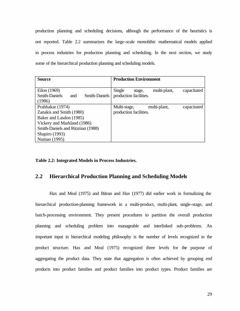
not reported. Table 2.2 summarizes the large-scale monolithic mathematical models applied
in process industries for production planning and scheduling. In the next section, we study
some of the hierarchical production planning and scheduling models.
Source Production Environment
Eilon (1969) Smith-Daniels and Smith-Daniels (1986)
Single stage, multi-plant, capacitated production facilities.
Prabhakar (1974) Zanakis and Smith (1980) Baker and Lasdon (1985) Vickery and Markland (1986) Smith-Daniels and Ritzman (1988) Shapiro (1993) Numao (1995)
Multi-stage, multi-plant, capacitated production facilities.
Table 2.2: Integrated Models in Process Industries.
2.2 Hierarchical Production Planning and Scheduling Models
Hax and Meal (1975) and Bitran and Hax (1977) did earlier work in formalizing the
hierarchical production-planning framework in a multi-product, multi-plant, single-stage, and
batch-processing environment. They present procedures to partition the overall production
planning and scheduling problem into manageable and interlinked sub-problems. An
important input in hierarchical modeling philosophy is the number of levels recognized in the
product structure. Hax and Meal (1975) recognized three levels for the purpose of
aggregating the product data. They state that aggregation is often achieved by grouping end
products into product families and product families into product types. Product families are

30
groups of products that share a common manufacturing set-up cost. Product types are groups
of families whose production quantities are to be determined by an aggregate production
plan. Families belonging to a type normally have similar costs per unit of production time
and similar seasonal demand patterns. In practical applications, more or fewer levels might
be needed. The hierarchical approach can be extended to different numbers of aggregation
levels by defining adequate sub-problems. Hax and Meal (1975) provide heuristics to
perform four levels of computations. First, products are assigned to plants using MIP, which
makes long-term capacity provision and utilization decisions. Second, a seasonal stock
accumulation plan is prepared using LP, making allocation of capacity in each plant among
product types. At the third level, detailed schedules are prepared for each product family
using standard inventory control methods, allocating the product type capacity among the
product families and at the fourth level, individual run quantities are calculated for each
product in each family, again using standard inventory control methods.
A significant aspect of the hierarchical approach is the ability of disaggregation
procedures to obtain feasible solutions of aggregate decisions at the detailed level. Bitran and
Hax (1977) conducted a series of experiments to examine the performance of the single-stage
hierarchical system to determine the size of the forecast errors, capacity availability,
magnitude of setup costs and nature of planning horizon. Bitran, Haas and Hax (1981)
compare various disaggregation procedures and analyze the impact of different aggregation
schemes on production planning costs. They also modify the procedures of Bitran and Hax
(1977) to incorporate high setup cost. Liberatore and Miller (1985) developed hierarchical
models for production planning and scheduling in single stage, multi-product capacitated
production facilities. They develop a LP model for production planning decisions and an MIP

31
for daily scheduling decisions. Their solution procedure is useful for single stage problems
only. Resource allocation in single stage, parallel machine scheduling application has been
described in Bitran and Tirupati (1988a,b). They develop mixed integer, quadratic program
aggregate planning model to homogenize the product group. This resulted in reduction in
complexity for the scheduling problem. Bowers and Jarvis (1992) applied hierarchical
framework for multi-product, single-stage production and scheduling problem. The three
phase models developed by Bowers and Jarvis implements inventory planning, short-term
production planning and daily sequencing tasks.
Meal (1978) describes an integrated distribution planning and control system citing
the complexities in extending the hierarchical approach to multistage systems. The two
stages are the parts production and assembly operations and the third stage is the distribution
system. This work lacks the consistency between aggregation and disaggregation procedures,
i.e., the link between the production and a distribution module is relatively weak. Gabbay
(1979) addressed multi-product, capacitated multi-stage production environment in
hierarchical planning framework. He does not provide a proposal to address the infeasibility
in production schedules. Bitran, Haas and Hax (1982) apply the extension of single stage
hierarchical stage production planning to two-stage production process. The two stages are
the parts production and the assembly process. Maxwell et al. (1983) propose a hierarchical
set of models for production planning in discrete parts manufacturing and assembly systems.
Their solution procedure works well with large capacity only. They apply the models in
stamping plants in US automotive industry. Bitran and Tirupati (1993) comprehensively
review the work done in single stage and multi stage hierarchical models in production
planning and scheduling. Ozdamar, Bozyel and Birbil (1998) develop hierarchical decision

32
support system for production planning in parts production and assembly process. They
develop models for planning at product type level, product family level and planning at end
product level. However, the disaggregation procedures suggested in this work do not
guarantee feasibility. Ozdamar and Yazgac (1999) propose hierarchical models for
production distribution system. In the planning model, Ozdamar and Yazgac consider
aggregation of time periods and products while omitting detailed capacity consumption by
setup. In table 2.3, we summarize the application of hierarchical models in discrete parts
manufacturing environment.
Bradley, Hax and Magnanti (1977) described an application of hierarchical
production systems to a continuous manufacturing process. Leong, Oliff and Markland
(1982) developed hierarchical models for production planning in process industries. They
apply the models in a fiberglass company with multi-product and parallel processor
production environment and report substantial cost savings. Oliff and Burch (1985) develop
three phase hierarchical models for production scheduling in process industries.
Source Production Environment
Hax and Meal (1975) Bitran and Hax (1977) Bitran, Haas and Hax (1981) Liberatore and Miller (1985) Bowers and Jarvis (1992) Bitran and Tirupati (1993)
Single stage, batch manufacturing systems
Bitran and Tirupati (1988a,b) Single Stage, Parallel Machine Gabby (1979) Bitran, Haas and Hax (1982) Maxwell et al. (1983) Bitran and Tirupati (1993) Ozdamar, Bozyel and Birbil (1998)
Multi-stage fabrication and assembly System
Meal (1978) Ozdamar and Yazgac (1999)
Multi-stage, Distribution and Planning System
Table 2.3: Hierarchical Models in Discrete Parts Manufacturing Industries

33
Lot sizes, line assignments and inventory levels are determined for individual products
through LP. Final job sequencing is accomplished by scheduling heuristics. Kleutgchen and
McGee (1985) developed mathematical models for Pfizer Pharmaceuticals. Implementation
of the models reduced inventories significantly. The main weakness in this work is that it is
restricted to inventory management and does not addresses other production planning and
scheduling decisions. Lin and Moodies (1989) develop two mathematical programming
models and sequencing heuristic for production planning and scheduling in steel industry.
Katayama (1996) propose a two stage hierarchical production planning system for process
industries. Katayama applies the hierarchical models in petrochemical plants with use of MIP
and neural network approach. Qiu and Burch (1997) develop hierarchical planning model for
production planning in process industries. MIP is developed for aggregate planning and sets
of heuristics are developed for daily scheduling. A brief summary of the work in hierarchical
production planning in process industries is given below in table 2.4. In the next section, we
review the research on scheduling with earliness and tardiness penalties.
Source Production Environment
Bradley, Hax and Magnanti (1977) Continuous manufacturing, job shop environment
Oliff and Burch (1985) Kleutghen and McGee (1985) Lin and Moodies (1989) Katayama (1996)
Multi-product, capacitated production facility, continuous production
Leong, Oliff and Markland (1982) Qiu and Burch (1997)
Multi-product, parallel machine
Table 2.4: Hierarchical Models in Process Industries
34
2.3 Earliness and Tardiness Scheduling
The study of earliness and tardiness penalties in scheduling models is a relatively
recent area of research. Most of the existing literature on scheduling focuses on problems that
have objective functions such as minimizing makespan (completion time of schedule) and
tardiness. Conway et al. (1967) refer to these objectives as regular performance measures,
and these measures are non-decreasing in completion times. Minimizing tardiness has been
the usual performance measure that considers the due dates of jobs. Recent interest in Just-
In-Time (JIT) production has created the notion that earliness, as well as tardiness should be
discouraged. The concept of penalizing both earliness and tardiness has resulted in new and
rapidly developing line of research in the scheduling field. As the use of both earliness and
tardiness penalties gives rise to a non-regular performance measures (non-increasing in
completion times), it has led to new methodological issues in the design of solution
procedures. The majority of research on earliness and tardiness scheduling is focused on
single machine scheduling, although some single machine models have been extended to
multi-machine setting. We begin by reviewing the research on single machine scheduling.
Single Machine Scheduling
Baker and Scudder (1990) review the research on single machine scheduling with
earliness and tardiness (E/T) penalties. Primarily, the literature has grown from the
generality of assumptions made about due dates and penalty costs. A generic E/T model is
defined in the following way. There are n jobs to schedule. Each job i is described by
processing time pi and a due date di. Scheduling decision would provide completion time of
job Ci. Earliness Ei and tardiness Ti of a job i is defined by Ei = max (0, di - Ci) and Ti = max

35
(0, Ci - di) respectively. Associated with each job i are earliness penalty, αi > 0 and tardiness
penalty, β i > 0. Assuming the penalty functions are linear, the basic objective function for
minimizing E/T costs, for any schedule S can be written as, ∑=
+=n
i
iiii TESf1
..)( βα . In some
formulations of the E/T problem, the due date is given, while in others the problem is to find
the optimal due date and the job sequence simultaneously. Allocating different penalties for
earliness and tardiness suggests that the associated cost components of both are different
from each other in many practical settings. However, all penalty functions are primarily to
guide the solution towards meeting the due date exactly. This implies that an ideal schedule
is the one in which all due dates are met exactly. An important special case in the family of
E/T scheduling problems is when αi = β i = 1, i.e., un-weighted E/T penalties. Common due
date of jobs is another notion in E/T scheduling. This represents situations where several jobs
belong to a single customer’s order or the assembly environment where components should
be ready at the same time to avoid production delays. The objective function in these special
cases becomes, minimizing the absolute deviation of job completion times from a common
due date, ∑∑==
−=+=n
i
i
n
i
ii dCTESf11
)(
One of the preliminary works on single machine E/T scheduling is by Sidney (1977),
who provides an efficient algorithm to minimize the maximum earliness or tardiness penalty.
This algorithm is improved by Lakshminarayan et al. (1978). The origins of a different
research direction can be traced to the work of Kanet (1981a). He considers the problem of
minimizing the total un-weighted earliness and tardiness around an unrestricted common due
date, i.e., due date that is not tight enough to act as a constraint on scheduling decision. E/T
36
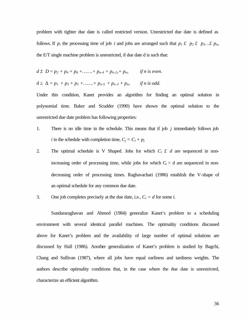
problem with tighter due date is called restricted version. Unrestricted due date is defined as
follows. If pi the processing time of job i and jobs are arranged such that p1 ≤ p2 ≤ p3…≤ pn,
the E/T single machine problem is unrestricted, if due date d is such that:
d ≥ ∆ = p2 + p4 + p6 +…….+ pn-4 + pn-2,+ pn, if n is even.
d ≥ ∆ = p1 + p3 + p5 +…….+ pn-5 + pn-3 + pn, if n is odd.
Under this condition, Kanet provides an algorithm for finding an optimal solution in
polynomial time. Baker and Scudder (1990) have shown the optimal solution to the
unrestricted due date problem has following properties:
1. There is no idle time in the schedule. This means that if job j immediately follows job
i in the schedule with completion time, Cj = Ci + pj
2. The optimal schedule is V Shaped. Jobs for which Ci ≤ d are sequenced in non-
increasing order of processing time, while jobs for which Ci > d are sequenced in non-
decreasing order of processing times. Raghavachari (1986) establish the V-shape of
an optimal schedule for any common due date.
3. One job completes precisely at the due date, i.e., Ci = d for some i.
Sundararaghavan and Ahmed (1984) generalize Kanet’s problem to a scheduling
environment with several identical parallel machines. The optimality conditions discussed
above for Kanet’s problem and the availability of large number of optimal solutions are
discussed by Hall (1986). Another generalization of Kanet’s problem is studied by Bagchi,
Chang and Sullivan (1987), where all jobs have equal earliness and tardiness weights. The
authors describe optimality conditions that, in the case where the due date is unrestricted,
characterize an efficient algorithm.

37
The restricted version of the problem occurs when common due date d < ∆. Hall,
Kubiak and Sethi (1991) have shown that the restricted version of single machine E/T
problem is NP-complete. Bagchi, Chang and Sullivan (1986) present an algorithm for solving
the restricted problem. However, their procedure implicitly assumes that the start time of the
schedule is zero. Szwarc (1989) proposes that the optimal start time may be nonzero, so that
the Bagchi, Chang and Sullivan algorithm does not guarantee optimality. The solution
procedures due to Szwarc (1989) and Bagchi, Chang and Sullivan (1986) are both
enumerative in nature. Sundararaghavan and Ahmed (1989) present a heuristic algorithm that
work effectively when the start time is zero. The worst case of enumerative approaches of the
solution procedures of restricted problem requires analysis of 2n schedules, where n is the
number of jobs.
Variants of E/T problems in single machine have been researched on the basis of
distinct due dates and weighted E/T penalties. Garey, Tarjan and Wilfong (1988) study the
problem of minimizing total un-weighted earliness and tardiness on a single machine with
distinct due dates of jobs. The single machine weighted earliness and tardiness scheduling
problem with distinct due dates is studied by Abdul-Razaq and Potts (1988). They provided a
branch and bound algorithm for the problem. For the same problem, Ow and Morton (1989)
provide a computational study of several heuristic algorithms. Li (1997) proposes lagrangian
relaxation based branch and bounds algorithms that guarantee the optimality of the solution,
the algorithms are useful for small problems only. Wan and Yen (2002) investigate single
machine E/T problem with distinct due dates and weighted E/T penalties. They develop
heuristic algorithms that have tabu search procedure and report computational performance
of heuristics. Ventura and Radhakrishnan (2003) focus on single machine E/T scheduling

38
with varying processing times and distinct due dates. They decompose the constraints in two
sets. One set of constraints, they solve as assignment problem, and relax the other set of
constraints to form the lagrangian dual problem. They solve the lagrangian problem using the
sub-gradient algorithm.
Some work is done on non-linear penalties in single machine E/T scheduling. Merten
and Muller (1972) introduced the completion time variance problem (CTVP) as a model for
file organization decisions in which it is important to provide uniform response times to
users. They also demonstrated the equivalence of the CTVP and the waiting-time variance
problem (WTVP). Schrage (1975) proposed the first exact algorithm for scheduling CTVP
up to 5 jobs. Eilon and Chowdhury (1977) provided an enumerative algorithm for
determining an optimal schedule when the number of jobs n is relatively small (n = 20).
Their algorithm minimizes WTVP. For large n, they proposed five heuristic procedures for
approximately solving the problem. Three of the heuristic procedures utilize pair wise
interchanges of adjacent jobs to improve the solution. Kanet (1981b) proved that CTVP is
equivalent to minimizing the sum of squared differences of job completion times. He adapted
an algorithm for the absolute deviation problem as a heuristic for the CTVP and showed that
the performance of his heuristic is superior to those proposed by Eilon and Chowdhury. Vani
and Raghavachari (1987) proposed heuristic algorithms for CTVP and claimed that their
heuristic procedure compares favorably with the heuristics of Eilon and Chowdhury and
Kanet. Bagchi et al. (1987) showed that the CTVP is equivalent to the mean squared
deviation problem (MSDP) of job completion times about some common due-date. They
noticed that for any given schedule, the optimal due date is equal to the mean completion
time. They proposed a branching procedure to find the optimal solution. Although they

39
utilized several dominance properties in order to accelerate their enumerative procedure, the
procedure is clearly inadequate for solving large problems (i.e., n = 20). Gupta et al. (1990)
proposed another heuristic, which is based on the complementary pair-exchange principle,
for finding a good approximate solution to the CTVP. Their heuristic procedure has been
shown through computational experiments to generate better solutions than other heuristics.
De et al. (1992) have presented a pseudo-polynomial dynamic programming algorithm for
optimally solving instances of the CTVP where processing times are small integers. They
also proposed a fully polynomial approximation scheme. Kubiak (1993) showed that the
CTVP is NP-complete. Kubiak (1995) proposed a quadratic integer programming
formulation and two new pseudo-polynomial dynamic programming algorithms for the
CTVP. In table 2.5, we provide taxonomy of the research done in single machine E/T
scheduling.
We now address the other class of problems in E/T scheduling which has the property
of inserted idle time.
Issue of Inserted Idle Time
Most of the E/T work in scheduling does not consider the issue of inserted idle time
(IIT) either by restricting the solution to be a non-delay schedule or by assuming a common
due date for all jobs. Inserted idle occurs when a resource is deliberately kept idle in the face
of waiting jobs. Kanet and Sridharan (2000) provide a comprehensive review of IIT
scheduling. However, they do not consider the review of Baker and Scudder (1990), as these
papers are restricted to non-IIT and non-delay schedules. For the n|1|di=d|ΣEi+Ti problem
(common due date problem), Cheng and Kahlbacher (1991) proved that it is unnecessary to
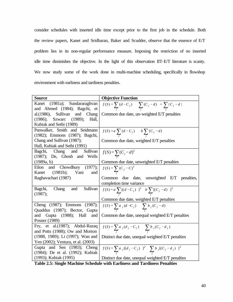
40
consider schedules with inserted idle time except prior to the first job in the schedule. Both
the review papers, Kanet and Sridharan, Baker and Scudder, observe that the essence of E/T
problem lies in its non-regular performance measure. Imposing the restriction of no inserted
idle time diminishes the objective. In the light of this observation IIT-E/T literature is scanty.
We now study some of the work done in multi-machine scheduling, specifically in flowshop
environment with earliness and tardiness penalties.
Source Objective Function Kanet (1981a); Sundararaghvan and Ahmed (1984); Bagchi, et al.(1986), Sullivan and Chang (1986); Szwarc (1989); Hall, Kubiak and Sethi (1989)
||)()()( dCdCCdSfj
jj
jj
j −=−+−= ∑∑∑ ++
Common due date, un-weighted E/T penalties
Panwalker, Smith and Seidmann (1982); Emmons (1987); Bagchi, Chang and Sullivan (1987); Hall, Kubiak and Sethi (1991)
∑∑ ++ −+−=j
jj
j dCCdSf )()()( βα
Common due date, weighted E/T penalties
Bagchi, Chang and Sullivan (1987); De, Ghosh and Wells (1989a, b)
Common due date, unweighted E/T penalties Eilon and Chowdhury (1977); Kanet (1981b); Vani and Raghavachari (1987)
∑ −=j
j CCSf 2)()(
Common due date, unweighted E/T penalties, completion time variance
Bagchi, Chang and Sullivan (1987);
22 ])[(])[()( ++ ∑∑ −+−=j
jj
j dCCdSf βα
Common due date, weighted E/T penalties Cheng (1987); Emmons (1987); Quaddus (1987); Bector, Gupta and Gupta (1988); Hall and Posner (1989)
∑∑ ++ −+−=j
jjjj
j dCCdSf )()()( βα
Common due date, unequal weighted E/T penalties
Fry, et al.(1987); Abdul-Razaq and Potts (1988); Ow and Morton (1988, 1989); Li (1997); Wan and Yen (2002); Ventura, et al. (2003)
∑∑ ++ −+−=j
jjjj
jjj dCCdSf )()()( βα
Distinct due date, unequal weighted E/T penalties
Gupta and Sen (1983); Cheng (1984); De et al. (1992); Kubiak (1993); Kubiak (1995)
∑∑ ++ −+−=j
jjjj
jjj dCCdSf 22 ])[(])[()( βα
Distinct due date, unequal weighted E/T penalties Table 2.5: Single Machine Schedule with Earliness and Tardiness Penalties
∑ −=j
j dCSf 2)()(

41
Multi-Machine Scheduling
Flowshop scheduling problems have attracted many researchers since the work of
Johnson (1954) for 2 machine flowshops. In flowshop problems, n jobs are processed on m
machines in the same order. We are going to review the research on flowshop scheduling that
has following assumptions. A machine processes only one job at a time; a job can be
processed on only one machine at a time; the operations are non-preemptable and setup times
of jobs on machines are independent of sequences. Since the early seventies, scheduling
researchers have been analyzing the computational complexity of various flowshop models.
NP-completeness of the flowshop problems minimizing makespan (completion time of
schedule) for m ≥ 3 has been shown by Garey et al. (1976), where m is the number of
machines. Koulamas (1994) has shown NP-hardness of F| | ΣTi problem for m ≥ 3. The above
complexity result coupled with the nature of flowshops has limited the possibility of
developing efficient solution algorithms for F2| | T. Sen, Dileepan and Gupta (1989)
proposed a branch-and-bound algorithm for F2 | | T. They first derived a local optimality
condition for sorting two adjacent jobs in a sequence that is sufficient, but not necessary. As
a result, this condition has a limited effect on reducing the size of the branch-and-bound
solution tree. Also Sen, Dileepan and Gupta lower bounds are rather weak because they are
based only on the tardiness of the already scheduled jobs and they do not include a lower
bound on the tardiness of the still unscheduled jobs. Kim (1993) proposed an improved
branch-and-bound algorithm for F2 | | T. Kim derived a condition for identifying jobs that
could be placed last in a optimal sequence which is analogous to Elmaghraby’s lemma for 1 |
| T. Kim developed stronger lower bound on the tardiness of the still unscheduled jobs.
However. Kim’s lower bounds are also weak because they are based on conservative

42
estimates on the completion time of the unscheduled jobs. The main drawback of the branch-
and-bound algorithms is that they do not utilize any dominance conditions for reducing the
size of the branch-and-bound solution tree. As a result, they can be applied only to small
problems with n < 15 jobs. Kim’s experiments also showed that his branch-and-bound
algorithm performs better than the algorithm of Sen, Dileepan and Gupta.
Since F| | ΣTi is NP- Hard, F| | ΣEi+Ti is also NP-Hard. The research on E/T penalties
in flowshop settings is very scanty. Gowrishankar et al. (2001) looked at minimizing the
completion time variance and the sum of squares of completion time deviations from a
common due date. They develop lower bound for both the problems. Using lower bound,
they propose branch and bound algorithms for the two problems. For larger problems, they
propose heuristics for both the problems. Other objective functions have not been looked in
flowshop E/T scheduling.
2.4 Research Gaps
In the previous sections, we have reviewed various production planning and
scheduling models applied to discrete parts manufacturing industries and process industries.
It is seen that models have been developed in single stage and multi-stage production
environment. Most of the models in multi-stage production environment have focused on
fabrication and assembly types of product structures. The production environment with
recycling process and its associated complexities has not been addressed in the literature. We
discussed in chapter 1, that recycling is an important issue in bringing down production costs.
We have studied the impact of recycling process on production planning and scheduling
decisions. The existing models on production planning and scheduling do not address the
43
complexities of the production environment we discussed in chapter 1. In integrated and
hierarchical models addressing production planning and scheduling decisions, inconsistency
often occurs in capacity requirements of production planning decisions and scheduling
decisions. Aggregate capacity of resources is considered in production planning decisions.
We discussed that while determining the scheduling decisions, infeasibilities may occur due
to excess capacity requirements. The complexities of the planning problem make scheduling
decisions even more difficult. The issue of alternate machines availability (resulting in
multiple routes of a product) is not addressed in the literature on multi-stage and multi-
machine environment. Also not addressed in the literature is the issue of backlogging of
demand over the planning horizon in multi-stage environment. This becomes an important
issue in situations when the schedule has tardiness.
In literature review of scheduling theory with earliness and tardiness (E/T) penalties,
we discussed reasons for considering earliness as a recent area of research. Most of the work
in E/T scheduling is limited to single machine scheduling with certain assumptions about the
due dates. Multi-stage environment like flowshop and jobshop production environment is
largely unattended in scheduling with E/T penalties. In the next chapter, we describe the
mathematical models to address the production planning and scheduling decisions.

44
3 Production Planning and Scheduling Models
3.1 Introduction
In this chapter, we describe the mathematical models that address the production
planning and scheduling decisions described in chapter 1. The production planning decisions
determine production quantity of products, inventory level of products and aggregate
capacity of production resources. The scheduling decisions determine the schedule of
products at each machine where they are processed. The schedule of a product comprises
start time and completion time of product at each machine.
We have seen in chapter 2 that modeling at different levels is called hierarchical
modeling in literature (Bitran and Hax, 1977; Bitran, Haas and Hax, 1981; Bitran and
Tirupati, 1993). We discussed that determining production planning and scheduling decisions
in one integrated model is computationally not efficient (Qiu et al., 1997). The motivation to
develop hierarchical models is also driven by the planning process observed in the
production environment. Production planning and scheduling decisions are required to be
made sequentially at increasing level of detail. Capacity requirements, timing and sizing of
production runs in the planning horizon are determined in production planning. Machine-
wise allocation of products to be produced is done in detailed scheduling. Hierarchical
modeling postpones the detailed scheduling decisions till they are actually required. The
detailed scheduling decisions are therefore, based on more accurate information. However,
there can be situations when the scheduling decisions are not feasible. The reason for this is
that aggregate capacity is considered at the time of determining production-planning
decisions. In scheduling, issues like job precedence constraints, and operation precedence

45
constraints may lead to capacity requirement, which is more than the available aggregate
capacity. This will result in an infeasible schedule. We will address the issue of infeasibility
in detail when we solve the production planning and scheduling problem.
We model the production planning and scheduling decisions in two steps. In the first
step, we model production-planning decisions. This is a mixed integer programme. The
decisions of the production-planning model over a finite planning horizon are:
− Quantity of each product to be produced on each production plant in each time period
− Inventory levels of finished goods, intermediate products, by-products and raw materials
in each time period
− Quantity of fresh raw material required in each time period.
The production-planning model also determines the aggregate capacity of the resources
required, in order to derive the production planning decisions.
In the second step, we model scheduling decisions. There are two scheduling models
to address scheduling decisions; one for finished goods scheduling and the other for
intermediate products scheduling. Detailed machine wise scheduling decisions, i.e., start
times and completion times of each product on each machine is derived from the scheduling
model. The rest of the chapter describes the formulation of production planning and
scheduling models. In the next section, we describe the formulation of production-planning
model. Mathematical formulations of scheduling models are discussed in section 3.3. We
summarize this chapter in section 3.4.
46
3.2 Production Planning Model
The production-planning model is developed for addressing medium range time
horizon decisions. The objective of the production-planning model is to minimize the
production costs. Production costs are the inventory costs and set up costs of end products,
intermediate products, inventory costs of by-products and recovered raw materials and cost
of fresh raw materials. We now provide the formulation of production planning model.
3.2.1 Formulation of Production Planning Model
The production-planning model is formulated as follows:
Indices
i = index of end products and intermediate products t = index of time period in the planning horizon j = index of the production plants m = index of by-products s = index of reusable raw materials that are recovered from by-products p = index of recycling plants u = index of reusable raw material storage tanks v = index of by-products storage tanks e = index of machines in the production lines r = index of routes of a product
Parameters
E = Set of end products, {i | i = 1,2,…,b} I = Set of intermediate products, {i | i = b+1,……,n} T = Set of time periods, {t | t = 1,2,……T} J = Set of production plants, {j | j =1,2,…..J} Ai = Set of products in bill of material of i, i ∈ E, I N = Set of machines used in the production plants, {e | e = 1,2,….N} Ri = Set of products (E and I) for which i is an input,{kaki>0, k ∈ E U I}. AR = Set of products that share machines but do not have alternate routes BR = Set of products that share machines but have alternate routes RTi = Set of routes of product i, i ∈ BR REe = Set of routes on machine e, e ∈ N

47
M = Set of by-products from which raw materials are recovered, {m | m =1,2,…,M} S = Set of raw materials which are recovered from by-products, {s | s = 1,2,…,S} P = Set of plants where by-products are processed to recover raw materials,
{p | p = 1,2,…P} TS = Set of tanks used for storing raw materials TM= Set of tanks used for storing by-products. As = Set of tanks used for storing raw material s, s ∈ S Bu = Set of raw materials stored in tank u, u∈TS Am = Set of tanks used for storing by-product m, m ∈ M Bv = Set of by-products stored in tank v, v∈TM aik = Amount of k required per unit of i, i ∈ E, I, k ∈ Ai.
rjt = Capacity (in hours) of production plant j in period t, j ∈ J, t ∈ T rejt = Capacity (in hours) of machine e in production plant j in time period t,
e ∈ N, j ∈ J, t ∈ T dit = Demand of product i in period t, i ∈ E Ci = Cost (in Rs per unit) of input materials to i, i ∈ E, I Sij = Setup cost for product i on phase j, i ∈ E, I, j ∈ J hi = Inventory cost (in Rs per unit) for product i, i ∈ E, I
= (Inventory carrying rate) * Ci tij = Time (in hours) to produce one unit of product i on production plant j,
i ∈ E, I, j ∈ J tiej = Time (in hours) to produce one unit of product i on machine e in production plant
j, i ∈ E U I, e ∈ N, j ∈ J τij = Setup time (in hours) for product i on production plant j, i ∈ E, I, j ∈ J Ni = Number of batches of product i that can be produced between two setups, i ∈ E, I Bi = Output batch size of product i, i ∈ E, I ssi = Safety stock of product i, i ∈ E, I ysmp = Ratio of raw material s recovered from by-product m at plant p,
s ∈ S, m ∈ M, p ∈ P cis = Amount of raw material s required per unit of i, i ∈ E, I, s ∈ S cpis = Minimum percentage of fresh raw material s required in product i, i ∈ E, I, s ∈ S Mmi = Amount of by-product m generated per unit of i, m ∈ M, i ∈ E, I Kmp = Processing capacity of plant p to process by-product m, m ∈ M, p ∈ P fpt = Available time (in hours) of plant p in time period t, p ∈ P, t ∈ T fs = Cost (in Rs) of fresh raw material s, s ∈ S hm = Inventory carrying cost (in Rs per unit per month) of by-product m, m ∈ M hs = Inventory carrying cost (in Rs per unit per month) of reusable raw material;
s, s ∈ S Am = Set of products generating by-product M = {iMmi>0} i ∈ E U I, m ∈ M Bs = Set of products using reusable raw material s = {icis>0}, i ∈ E U I, s ∈ S Cu = Capacity of tank u, u ∈ TS Cv = Capacity of tank v, v ∈ TM

48
Variables
Xijt = Quantity of product i produced on production plant j in time period t, i ∈ E, I, j ∈ J, t ∈ T
XRirjt = Quantity of product i on route r on production plant j in time period t, i ∈ E U I, r ∈ RTi, j ∈ J, t ∈ T
Iit = Inventory of product i at the end of period t, i ∈ E, I, t ∈ T Oijt = Number of setups of product i on production plant j in time period t,
i ∈ E, I, j ∈ J, t ∈ T Yst = Reusable raw material s used at all production plants in period t, s ∈ S, t ∈ T Fst = Quantity of fresh raw material s used at all production plants in period t,
s ∈ S, t ∈ T Fsit = Quantity of fresh raw material s used in product i at all production plants in
period t, s ∈ S, i ∈ E, I, t ∈ T Qmpt = Quantity of by-product m processed at plant p in period t, m ∈ M, p ∈ P, t ∈ T ISst = Inventory of reusable raw material s at the end of period t, s ∈ S, t ∈ T ISTsut = Inventory of reusable raw material s in tank u at the end of period t,
s ∈ S, u ∈TS, t ∈ T IMmt = Inventory of by-product m at the end of period t, m ∈ M, t ∈ T IMTmvt = Inventory of by-product m in tank v at the end of period t, m ∈ M, v ∈TM, t ∈
T
∑∑ ∑∑ ∑∑ ∑∑ ∑∑++++=i t i t s t m t s t
stsmtmstijtijiti FfIMhIShsOSIhz ... min ..
subject to:
∑ −+= −
j
itijtitit dXII 1 ∀ i,t. i∈ E (1)
.1 ∑∑∑∈
−+= −
Rik j
kiijt
j
ijtitit aXXII ∀ i,t. i∈ I (2)
).( .∑ ≤+i
jtijijtijijt rOtX τ ∀ j,t. i∈ E,I (3)
) ( ).( .. .∑ ∑ ∑∈ ∈ ∈
≤+++ARi
ejt
BRi
ijijt
REr
iejirjtijijtiejijt rOtXROtXe
ττ ∀ e, j,t (4)
∑∈
=iRTi
irjtijt XRX ∀ i,j,t. i∈ E,I (5)
.. iiijtijt BNOX ≤ ∀ i, j,t. i∈ E,I (6)
iit ssI ≥ ∀ i,t. i∈ E,I (7)
∑ ∑∈
−+= −
Mm P
stsmpmptstst YyQISIS .1 ∀ s,t.. (8)
∑∑ ∑∈
− −+=MAi j
Pmptmiijtmtmt QMXIMIM .1 ∀ m,t. i∈ E,I (9)

49
∑ ∑∈
=+j Bi
isijtstst
S
CXFY . ∀ s,t. i∈ E,I (10)
.. ∑≥j
ijtpisissit XccF ∀ s,i,t. i∈ E,I (11)
st
i
sit FF =∑ ∀ s,t. (12)
∑ ≤M
ptmpmpt fkQ . ∀ p,t. (13)
∑∈
≤us
usut
BCIST ∀ u,t .u∈ TS (14)
∑∈
=su
stsut
AIIST ∀ s,t. (15)
∑∈
≤vm
vmvt
BCIMT ∀ v,t. v∈ TM (16)
∑∈
=MA
IIMTv
mtmvt ∀ m,t. (17)
integerOQFFYIMTISTIMISIX
ijt
mptsitststmvtsutmtstitijt
, 0,,,,,,,, ≥ (18)
Constraint 1 indicates that demand for each end product has to be met in each time
period. Constraint 2 is for derived demand of intermediate products. It indicates that demand
of each intermediate product in each time period is based on the production of intermediate
and end products where the product is an input. Constraint 3 is the capacity constraint of
dedicated production plants. It restricts the production quantity of intermediate and end
products produced on the basis of available capacity of plants in each time period. Constraint
4 is the capacity constraint of flexible production plants. The first summation in the
constraint is capacity required in each time period for processing and setups of products that
share machines but do not have alternate routes. The second summation is for the capacity
requirement in each time period of products that share machines and have alternate
production routes. Constraint 5 sums the total production of a product across all its routes in
each time period. Constraint 6 ensures that the required numbers of setups are done in one
production run of a product in each production plant in each time period. Constraint 7

50
provides lower bounds on the inventory levels of end products and intermediate products in
each time period. Constraint 8 is the inventory balance for recovered raw materials. It states
that in each time period recovered raw materials are generated by processing of by-products
and are consumed in production of intermediate and end products. Constraint 9 is the
inventory balance constraint for by-product. It indicates that in each time period the by-
products are generated by intermediate and end products produced and are consumed in the
recycling plants to recover raw materials. Constraint 10 is the total raw material requirement
in each time period, i.e., the sum of fresh raw material and recovered raw material would be
the total requirement of raw material across all products. Constraint 11 is for minimum
quantity of fresh raw materials required in each time period. It provides a lower bound on the
use of fresh raw material for each product. Constraint 12 equates that the total fresh raw
material consumption in each time period to the fresh raw material consumed across all
products. Constraint 13 restricts the processing of by-products in each time period on the
basis of available capacity of recycling plants. Constraint 14 limits the inventory of recovered
raw material in each time period with the storage tank capacity. Constraint 15 equates the
sum of inventory of recovered raw material in each tank to its total inventory in each time
period. Constraint 16 restricts the inventory of by-products in each time period with the
available storage tank capacity. Constraint 15 states that inventory of by-products in each
tank in each time period is equal to its total inventory. In the next section, we describe the
formulations of finished goods scheduling model and intermediate products scheduling
model.

51
3.3 Scheduling Models
In this section, we describe the formulations of scheduling models in order to derive
scheduling decisions of the production planning and scheduling problem. The scheduling
decisions determine start time and completion time of a job at each machine. The aggregate
production plan derived from the production-planning model is input to the scheduling
model. The production plan of the planning model imposes constraints on the scheduling
model.
Scheduling problem consists of two parts, one is the finished goods scheduling and
the other is the intermediate products scheduling. They are different problems because the
production environment is different in finished goods and the intermediate products. As
discussed in chapter 1, finished goods in our problem have flowshop pattern. In a flowshop,
each product has same sequence of operations. For determining the optimal schedule of any
performance measure, jobs may or may not be processed in the same sequence at each
machine. If jobs are processed in the same sequence at all machines, the flowshop is known
as permutation flowshop. Finding an optimal schedule in a flowshop for any objective when
sequence of jobs may vary at machines is significantly harder than for determining the
sequence for permutation flowshop (Baker, 1974; Pinedo, 1998). As a result, we have
considered the permutation flowshop production environment in the scheduling problem.
The finished goods have a due date that is specified by the customer orders and
demand forecast. One of the objectives of the scheduling model is to meet the customer
orders with minimum tardiness. Tardiness of a job Ti is defined as: Ti = max (C i – di, 0),

52
where Ci is the completion time of job i on the last machine and di is the due date of job i.
Tardiness is a regular performance measure, i.e., non-decreasing in Ci for all i. Garey,
Johnson and Sethi (1976) provide NP-hardness proof of the m machine permutation flowshop
tardiness problem. In a multi-stage environment, minimizing inventory costs also becomes
important as inventory costs are incurred at various stages of producing finished goods in the
form of intermediate products. Also some intermediate products have limited shelf life. Thus
minimizing earliness is also one of the objectives of the scheduling model. Earliness of a job
Ei is defined as: Ei = max (di – Ci, 0). Earliness is a non-regular performance measure, i.e.,
non-increasing in Ci for all i. The overall objective of the scheduling model is to minimize
earliness and tardiness (E/T) penalties, i.e., to minimize absolute deviation of job completion
times about their due date. The flowshop E/T problem is harder than the flowshop tardiness
problem, hence we focus on analyzing special case of flowshop E/T problem which has
common due date of jobs.
We now provide the formulation of permutation flowshop problem of minimizing
earliness and tardiness penalties with common due date d. This is the MIP model for finished
goods scheduling decisions.
3.3.1 Finished Goods Scheduling Problem Formulation
Indices i = index of jobs j = index of machines Sets N = set of jobs, {i | i=1,2,…..,n} S = set of machines, {j | j=1,2,….,m}

53
Parameters d = common due date of jobs pij = processing time of job i on machine j Variables Sij = start time of job i on machine j Cij = completion time of job i on machine j Ti = tardiness of job i, Ti= max(Cim-d, 0) Ei = earliness of job i, Ei = max(d-Cim, 0) yik = 1, if job i is before job k in a sequence, i, k∈ N 0, otherwise bi = 1, if Ti ≥ 0 0, otherwise
∑ ∑ −=+=i i
imii dCTEZ min
subject to:
1 ijijij pCC +≥ − ∀ i∈ N, j∈ S (1)
)1( kjikijkj pyMCC ≥−+− ∀ i, k∈ N, j ∈ S (2)
ijikkjij pyMCC ≥+− ∀ i, k∈ N, j ∈ S (3)
iiim ETdC −=− ∀ i∈ N (4)
ii bMT ≤ ∀ i∈ N (5)
)1( ii bME −≤ ∀ i∈ N (6)
ijijij pSC += ∀ i∈ N, j ∈ S (7)
0,,, ≥iiijij TESC (8) { } 0,1 , ∈iik by Constraint 1 is operation precedence constraint for a job. It ensures that an operation
cannot start until the previous operation is complete. Constraint 2 and constraint 3 indicate

54
job precedence at a machine. They ensure that if a job i is scheduled before job k, then at
each machine job k is started only after job i is completed. Constraint 4 determines Ei or Ti of
a job, as the case may be. Constraint 5 and constraint 6 ensure that only one of Ei or Ti is
incurred as by definition Ei = -Ti and both Ei and Ti are non-negative. Constraint 7 indicates
that preemption is not allowed for a job and determines the start times of each job at each
machine.
Finished goods have external demand in the form of customer orders and forecast.
Intermediate products have derived demand based on the production of products, where
intermediate products are inputs. Finished goods derive their due dates from customer orders.
Intermediate products derive their due dates from the production schedule of products where
they are required. In our problem the production process of finished goods and intermediate
products differ on the basis of production routes. As we have seen, finished goods follow
flowshop pattern whereas intermediate products have general route, similar to jobshop
environment. In a jobshop, each product has a distinct route that may or may not be similar to
the route of other products. An intermediate product in our problem has an additional
complexity that it may require a particular machine several times in its route, i.e., job shop
with re-entrant flows. We now provide the formulation of scheduling model for intermediate
products scheduling.
3.3.2 Intermediate Products Scheduling Problem Formulation
Indices i, k = index of jobs j = index of machines l, s = index of operations

55
Sets N = set of jobs, {i | i=1,2,…..,n} S = set of machines, {j | j=1,2,….,m} Parameters d = common due date of jobs
sie = machine used by job i for sth operation
pij = processing time of job i on machine j Li = last operation of job i Variables Sij = start time of job i on machine j Cij = completion time of job i on machine j Ti = tardiness of job i, Ti=max (Cim-d, 0)
Ei = earliness of job i, Ei = max (d-Cim, 0)
yilkse = 1, if lth operation of job i is before sth operation of job k at machine e i, k∈ N, e∈ S 0, otherwise
bi = 1, if Ti ≥ 0 0, otherwise
∑ ∑ −=+=i i
Liieii dCTEz imin
subject to:
1 l
iieliie
liie pCC ≥−
− ∀ i∈ N, j∈ S (1)
)1( kjilskeijkj pyMCC ≥−+− ∀ i,k∈ N, j ∈ S (2)
ijilksekjij pyMCC ≥+− ∀ i,k∈ N, j ∈ S (3)
iiLiie ETdC i −=− ∀ i∈ N (4)
ii bMT ≤ ∀ i∈ N (5)
)1( ii bME −≤ ∀ i∈ N (6)
ijijij pSC += ∀ i∈ N, j ∈ S (7)
0,,, ≥iiijij TESC (8) { } 0,1, ∈iilkse by
56
Constraint 1 indicates that an operation of a job can be started only after its previous
operation is completed. Constraint 2 and 3 ensure that there is no overlapping of jobs at a
machine. They indicate that if at machine j, lth operation of job i is scheduled, then sth
operation of another job k can be started only when job i has finished processing on machine
j. Constraint 4 determines the earliness and tardiness of each job. Constraint 5 and constraint
6 ensure that only one of Ei or Ti is incurred as by definition Ei = -Ti and both Ei and Ti are
non-negative. Constraint 7 indicates that preemption of job is not allowed and determines the
completion time of each job. We now summarize this chapter.
3.4 Summary
In this chapter we have described the mathematical models to address the decisions of
production planning and scheduling problem considered in this research. We have discussed
the reason for modeling the decisions sequentially through hierarchical models. The
production planning is a mixed integer linear programming model. We have developed two
scheduling models, one for finished goods scheduling and the other for intermediate products
scheduling. Both scheduling models are mixed integer linear programming models. In the
next chapter we describe the solution algorithms for solving the production planning and
scheduling problem.

57
4 Solution Procedure for Production Planning and Scheduling Problem
4.1 Introduction
We have modeled the production planning and scheduling decisions in chapter 3 in
two steps. In the first step, we have developed the production-planning model as a mixed
integer programme (MIP). The decisions of the production-planning model are production
quantities of products, inventory levels of products and aggregate capacity of resources
required to meet the production plan. In the second step, we have modeled scheduling
decisions, which are start times and completion times of each product on each machine.
Scheduling problem consists of two parts, finished goods scheduling and intermediate
products scheduling. Finished goods follow flowshop pattern of production process. In
chapter 3, we presented an MIP formulation for finished goods scheduling problem.
Intermediate products follow a general job shop pattern of production process with re-entrant
flows. In chapter 3, we also presented an MIP formulation of intermediate products
scheduling problem. We discussed in chapter 3, the rationale for modeling the production
planning and scheduling decision in a hierarchical manner. The decisions of production-
planning model are constraints, within which, the detailed scheduling decisions are made.
The decisions of the production planning model, production quantity and inventory levels of
products, are input parameters to the detailed scheduling model.
In this chapter, we discuss the solution procedure for solving the production planning
and scheduling problems. In section 4.2, we define the framework that we have used to solve
the production planning and scheduling problem. In section 4.3, we provide the solution

58
procedure for production-planning problem. Next, we develop solution procedures for
solving the scheduling problems. In section 4.4, we develop the solution procedure for
solving the finished goods scheduling problem. In section 4.5, we solve the intermediate
products scheduling problem. We discussed in chapter 1, that the production environment has
dedicated production plants. In section 4.6, we describe the solution procedure solving the
dedicated plant-scheduling problem. We summarize this chapter in section 4.7.
4.2 Solution Procedure for Production Planning and Scheduling Problem
As we discussed in section 4.1, we are solving production planning and scheduling
problem in two steps. In the first step, we solve the production-planning problem as shown in
figure 4.1. Production quantities of products and inventory levels of products are the
decisions of production planning model. Production planning decisions are input to the
scheduling model. The scheduling model has to determine the schedule of production plan
proposed by the production-planning model. In the second step, we develop solution
procedure for solving finished goods scheduling problem. We develop analytical results and
heuristics for solving the finished good scheduling problem. Then, we develop solution
procedure for intermediate products scheduling problem. We report results of the solution
procedure for the production planning and scheduling problem in chapter 5. In the next
section, we describe the solution procedure for production planning problem
4.3 Solution Procedure for Production Planning Problem
The production-planning model is solved using the branch and bound algorithm.
Demand for finished goods in each period of the planning horizon is an input to the model.
Aggregate capacity is considered in the production-planning model. For dedicated plants,
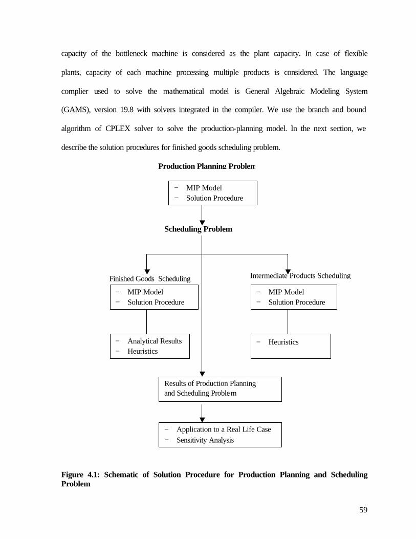
59
capacity of the bottleneck machine is considered as the plant capacity. In case of flexible
plants, capacity of each machine processing multiple products is considered. The language
complier used to solve the mathematical model is General Algebraic Modeling System
(GAMS), version 19.8 with solvers integrated in the compiler. We use the branch and bound
algorithm of CPLEX solver to solve the production-planning model. In the next section, we
describe the solution procedures for finished goods scheduling problem.
Figure 4.1: Schematic of Solution Procedure for Production Planning and Scheduling Problem
Intermediate Products Scheduling Finished Goods Scheduling
− MIP Model − Solution Procedure
Scheduling Problem
− Analytical Results − Heuristics
− MIP Model − Solution Procedure
− Heuristics
− Application to a Real Life Case − Sensitivity Analysis
− MIP Model − Solution Procedure
Results of Production Planning and Scheduling Problem
Production Planning Problem

60
4.4 Solution Procedure for Finished Goods Scheduling Problem
As we discussed in chapter 3, that to solve finished goods scheduling problem, we are
considering permutation flowshop with common due date. The objective of the scheduling
model is to minimize earliness and tardiness (E/T) penalties. We discussed in chapter 2, that
the existing results on earliness and tardiness penalties have focused on single machine
scheduling. We also discussed the unrestricted due date in single machine scheduling (Baker
and Scudder, 1990). Let us call the unrestricted due date for single machine as d0. Let d be
the common due date for all the jobs. When jobs are arranged such that p1 ≤ p2 ≤
……………≤.pn, a problem is called unrestricted if:
d ≥ d0 = ( pn + pn-2 + pn-4 +…….+ p4 + p2), if n is even.
d ≥ d0 = (pn + pn-2 + pn-4 +…….+ p3 + p1), if n is odd. For any value of d < d0, the problem
is restricted Let SUD(d) be the single machine E/T problem for common due date d ≥ d0.
Baker and Scudder (1990) have derived the optimal sequence, properties of optimal sequence
and the schedule of SUD(d). The optimal sequence of SUD(d) for common due date d ≥ d0 is:
(n, n-2, n-4,…..,1,..,2,.... 4,…….n-3, n-1), if n is odd
(n, n-2, n-4,…..,2,..,1,….3,…….n-3, n-1), if n is even. The properties of optimal sequence of SUD(d) are:
a) No idle time between jobs in the schedule.
b) V-shaped optimal sequence. In a V shaped sequence, jobs scheduled before the due
date d are in longest processing time first (LPT) sequence and jobs scheduled after d
are in shortest processing time first (SPT) sequence.
c) One job finishes at due date d.

61
To determine the schedule of the optimal sequence obtained above for common due
date, d ≥ d0, let Si and Ci be the start time and completion time of job i respectively. If the
optimal sequence is 1,2,…e-1, e, e+1,….n, where e is the job that finishes at common due
date d, i.e., Ce = d and Se = Ce - pe. There is no idle time in this schedule, Ce-1 = Se and Se-1
= Ce-1 – pe-1. This way the schedule of the optimal sequence is determined.
We use these results of single machine E/T problem for unrestricted common due
date and exploit some of its properties in solving special cases of multi-machine problems. In
multi-machine problems, we are studying permutation flowshop with common due date,
which is a more tractable case of flowshop environment. Next, we develop the unrestricted
and restricted due dates for permutation flowshops with common due date.
We would like to begin by stating that there could be alternate optimal sequences of
SUD(d) for any d > d0. The optimal sequence shown above is at d = d0. This optimal
sequence is:
(n, n-2, n-4,…..,1,..,2,.... 4,…….n-3, n-1), if n is odd
(n, n-2, n-4,…..,2,..,1,….3,…….n-3, n-1), if n is even.
No matter what the optimal sequence is, the cost of the schedule of any of the alternate
optimal sequences is obviously same. It is difficult to obtain all alternate optimal sequences
for d > d0. However, all the alternate optimal sequences can be obtained for SUD(d) at d =
d0. The set of all alternate optimal sequences at d = d0 would be used later to solve flowshop
E/T problem, hence we now describe a procedure to generate all alternate optimal sequences
at d = d0. It is to be noted that there will be alternate optimal sequences at d = d0, only if,

62
processing times of any two jobs are same. The alternate optimal sequences at d =d0 are
generated as follows. If the optimal sequence obtained above is index from 1 to n,
Procedure for Generating Alternate Optimal Sequences at d =d0 (GAOS) Step 1: j = 1
Step 2: x = j +1
Step 3.1: Is pxm = pjm
Yesà Create new sequence by interchanging j and x x = x + 1 is x = n +1
yesà j = j + 1 and goto step 3.2 noà repeat step 3.1
Noà x = x + 1 and repeat step 3.1 Step 3.2 if j = n STOP else goto step 2
We now define some terms before deriving unrestricted and restricted due dates for
flowshop E/T problem.
Notation i = index of jobs, i =1,2,…n. j = index of ordered machines in a flowshop, j=1,2…..m. s = index of sequences of jobs, s = 1,2,…l d = common due date of jobs pij = processing time of job i on machine j d0 = unrestricted common due date for single machine,
pnm + pn-2m + pn-4m +…….+ p4m + p2m , if n is even pnm + pn-2m + pn-4m +…….+ p3m + p1m , if n is odd. SUD(d0) = single machine E/T problem for unrestricted common due date d0
S(m, d0) = set of optimal sequences of SUD(d0) at last machine m with common due date d0. S(m, d0) is generated by procedure described above of generating optimal sequences.
E(s, d0) = set of early and on-time jobs in sequence s with common due date d0,
s∈ S (m, d0).
T(s, d0) = set of tardy jobs in sequence s with common due date d0, s ∈ S (m, d0).

63
r(s, d0) = schedule of optimal sequence s, consisting of Si and Ci ∀i, s∈ S (m, d0). Schedule is generated as described in the procedure above in this section, when we discussed the single machine results from Baker and Scudder (1990).
Ζ1{r (s, d0)} = earliness and tardiness costs of schedule r (s, d0). Sij = start time of job i on machine j Cij = completion time of job i on machine j F(s) = Flowshop schedule of sequence s, s ∈ S(m,d0). F(s) is determined as follows.
Let the sequence be 1,2,……n. S11 = 0, for i = 1 to n
for j = 1 to m,
Sij = max {C ij-1, Ci-1j} Cij = Sij + pij MF(s) = Makespan of schedule F(s), MF(s) = Cnm , s ∈ S (m, d0). This is the completion
time of last job in the sequence. Makespan of the schedule is defined as the completion time of last job in the sequence. MF(s)
is the makespan of schedule F(s) of permutation flowshop sequence s. We define k as the
sequence with minimum makespan, i.e., )(),( 0
min arg sFdmSs
Mk∈
= . The unrestricted due date d1 in
permutation flowshop environment is defined as ∑∈
−=),(
)(1
0dkTj
jmkF pMd . The first term at right
hand side is the makespan of sequence k. The second term is the sum of tardy jobs in
sequence k. Now we develop the restricted due date d2 in permutation flowshop setting. Let
us define: nipam
j
iji
,....2,1 minarg1
∑=
=∀= . a is the minimum of sum of processing times of
job at all machines amongst all jobs. We call this sum as the restricted due date, i.e.,
d2 = 1
∑=
m
j
ojp

64
We have defined in the above paragraphs, the unrestricted due date d1 and restricted
due date d2 in a permutation flowshop environment. We now define another range of due
date, that is in between the restricted and unrestricted due date, and we call it as intermediate
due date. Thus, for flowshop E/T problem for common due date, we have problems for d ≥
d1(unrestricted due date); d2 < d < d1 (intermediate due date) and d ≤ d2 (restricted due date).
On the basis of the classification of due dates, we have decomposed the flowshop E/T
problem into three sub problems as shown in figure 4.2.
Figure 4.2: Flowshop E/T Problem Decomposition Based on Due Dates
Sub-problem 1 is the flowshop E/T problem defined over the unrestricted common
due date d ≥ d1, sub-problem 2 is flowshop E/T problem defined over the intermediate due
date d2 < d < d1 and sub-problem 3 is the flowshop E/T problem defined over the for
restricted due date d ≤ d2. Sub-problem 3 has a special structure by definition of d2, that all
jobs will be necessarily tardy. We will discuss in detail about the special properties of sub-
problem 3 when we will describe the solution procedure for solving sub-problem 3 later in
this chapter. In the following sub-sections, we describe each of the sub-problems and
solution algorithms to solve them. In sub-section 4.4.1, which follows next, we solve sub-
problem 1.
Unrestricted Due date Problem Sub Problem 1
d2 d1
d ≥ d1 d2 < d < d1 d ≤ d2
Intermediate Due date Problem Sub Problem 2
Restricted Due date Problem Sub Problem 3

65
4.4.1 Sub-Problem 1: Flowshop E/T Problem for Unrestricted Common Due Date
In this sub-section, we develop the solution procedure for solving the permutation
flowshop E/T problem for unrestricted common due date d ≥ d1. The objective of sub-
problem 1 is to minimize E/T penalties, i.e., ∑ ∑ −=+=i i
imii dCTEZMinimize , where Cim
is the completion time of job i on the last machine m.
One of the optimal properties of SUD(d) is that there is no idle time in the schedule. If
there is an idle time, it should be removed while maintaining the feasibility of the schedule.
We now develop a procedure to remove idle time in the schedule F(s) at the last machine.
This procedure will be used later in the solution procedure for solving sub-problem 1.
Procedure for Removing Idle Time at Last Machine (RIT) Let the sequence s be 1,2,….n .
Step 1: i = n
Step 2: t = Sim-Ci-1m
Step 3: If t > 0 Yesà for x = 1 to i-1 Sxm = Sxm + t Cxm = Sxm + pxm If i = 1, STOP else i = i –1 and goto Step 2 Noà If i = 1, STOP else i = i –1 and goto Step 2
In step 1, the last job in the sequence is selected. Step 2 checks if there is an idle time
between the jobs. Step 3 removes the idle time between the jobs while maintaining the
feasibility of the schedule. This procedure would result in following schedule at machine m.

66
Cnm = MF(s) Snm = Cnm-pnm For i = n-1 to 1 Cim = Si+1.m Sim = Cim – pim
We now state a theorem to determine optimal solution for sub-problem 1.
Theorem 1: For a flowshop E/T problem with common due date d ≥ d1, there is an optimal
sequence k with Z{F(k)} = Z1{r(k,d0)}.
Proof: By definition of SUD(d0), sequence k is optimal for d ≥ d0. It follows that for d
≥ d0, Z1{r(k, d)} = Z1{r(k,d0)}. By definition, d1 ≥ d0. Thus for d ≥ d1, sequence k is optimal
for SUD(d) and Z1{r(k,d1)} = Z1{r(k,d0)}. Z{F(k)} is function of completion time of jobs at
machine m, i.e., ∑=
−=Ζn
j
jm dCkF1
1)}({ for d = d1. It follows that Z{F(k)}≥ Z1{r(k,d1)} as
Z1{r(k,d1)} is optimal for d = d1.
In schedule F(k) at machine m, if Sim = Ci-1.m ∀ i = n, n-1, n-2,….,2, sequence k has
all optimal properties of SUD(d) at d = d1. If Si.m ≥ Ci-1.m ∀ i = n, n-1, n-2,….,2, this idle time
can be removed by the procedure RIT defined above.
It follows that sequence k has now all properties of SUD(d) at d = d1. Thus, Z{F(k)} =
Z1{r(k, d)} at d = d1. If d1 is increased to d1 + ∆, the optimal schedule at stage m would be Cim
= Cim + ∆ for i = n-1 to 1 and Cnm = MF(k) + ∆. For d > d1, all properties of SUD(d) hold.
Hence for d ≥ d1, Z{F(k)} = Z1{r(k, d0)} and sequence k is optimal.
Q.E.D.

67
We have derived above optimal solution for sub problem 1. We would like to state
that the value of unrestricted due date d1 in sub problem 1 is determined on the basis of set of
all optimal sequences of single machine E/T problem at d = d0. As mentioned earlier in
section 4.4, it is difficult to obtain optimal sequences for single machine E/T problem for d >
d0. In that sense the value of d1 could be made tighter. This is because some of the optimal
sequences for d > d0 could have lesser makespan than MF(k), and d1 is a function of MF(k) as
defined above. In the next sub section we describe sub problem 2 and develop its solution
procedure.
4.4.2 Sub-Problem 2:Flowshop E/T Problem for Intermediate Common Due Date The objective of sub problem 2 is same as that of sub-problem 1, i.e.,
∑ ∑ −=+=i i
imii dCTEZMinimize . The difference between sub problems 1 and 2 is in the
value of the common due date d. The common due date value for sub problem 2 is between
d2 and d1, i.e., d2 < d < d1. Garey et al. (1976) provide proof of NP-completeness of this
problem. We were able to use some of the optimal properties of single machine E/T problem,
and construct optimal results for flowshop E/T problem for d ≥ d1. For common due date d <
d1, we find that it is difficult to obtain analytically optimal solution for flowshop E/T
problem. We have developed a heuristic algorithm to solve sub-problem 2. We now describe
the proposed heuristic algorithm to solve sub problem 2.
4.4.2.1 Heuristic Algorithm (H1) for Sub Problem 2
The proposed heuristic for solving sub-problem 2 is based on permutation sequence
of jobs at the bottleneck machine. Bottleneck machine is identified in this problem as the
machine that requires maximum sum of processing time of all jobs amongst all machines.

68
The solution of multi-machine problems is often useful by decomposing the problem into
single machine problems. As a result, we solve the single machine E/T problem at the
bottleneck machine. The pre-bottleneck processing times of a job is captured by considering
release dates of job at the bottleneck machine. The release date of a job in this problem is
defined as the earliest time at which the job is available for processing at the bottleneck
machine. The post-bottleneck processing times of a job is captured by determining the due
date of a job at the bottleneck. The resulting problem is single machine E/T problem with
release dates and distinct due dates, n/1/ri/Σ(Ei+Ti). We solve this single machine problem at
the bottleneck machine. To solve this, we refer some results on n/1/ri/Σ(Ei+Ti by Chu (1992)
and Chu and Portmann (1992). They derive a sequence of jobs on single machine. In our
heuristic, using a priority function (defined below in the detailed heuristic steps), a job is
selected and appended to a partial sequence. Schedule of the partial flowshop sequence is
developed (explained below). Based on this schedule, release dates and due dates of a job are
updated at each iteration of appending the job. The schedule of the complete permutation
sequence is then modified to improve earliness and tardiness costs. In the end, local
neighborhood search procedure (tabu search) is applied to improve the solution. We now
explain the detailed steps of the heuristic.
Notation d = common due date for all jobs i = index of jobs, i = 1,2,…n j = index of machines, j = 1,2,…m pij = processing time of job i on machine j k = bottleneck machine Sij = start time of job i on machine j Cij = completion time of job i on machine j rik = earliest time at which job i is available for processing at machine k dik = due date of job i at bottleneck machine k σ = a permutation flow shop sequence of n jobs

69
π = set of partial sequence of jobs s(σ, i) = schedule of sequence σ consisting of Sij and Cij for ∀ i∈σ, j =1,2,…,m Z{s(σ, i)} = cost of permutation flowshop schedule
Z{s(σ, i)} = ∑=
n
i 1
Cim - d
The problem is to determine σ and s(σ, i) so as to minimize Z{s(σ, i)}.
Heuristic (H1) for Solving Sub-Problem 2
Step 1 Determining bottleneck machine k
∑=
=n
i
ijj
pk1
maxarg
Step 2 Determining permutation flowshop sequence (σ) and schedule s(σ, i) for σ
Step 2.1 Determining release date of job i at bottleneck machine k
1,2,...ni 1
1
=∀= ∑−
=
k
x
ixik pr
Determining due date of job i at bottleneck machine k
1,2,...ni 1
=∀−= ∑+=
m
kx
ixik pdd
Step 2.2 Determining priority ui of jobs
ui = rik if rik + pik ≥ dik
ui= dik – pik if rik + pik < dik
Step 2.3 Appending a job to π (partial sequence)
Select job with minimum ui and add to π
Step 2.4 Schedule s(π , i) as follows:
for i to |π |, i∈ π ,

70
for j = 1 to m
S11 = 0
Sij = max {Cij-1, Ci-1j}
Cij = Sij + pij
Step 2.5 Updating rik ∀ i ∉ π
Add i to π and call it π i
Determine s(πi, i) according to step 2.3 ∀ i ∈ πi, j = 1 to m
rik = Cπi k-1(completion time of i at (k-1) after being appended to π)
This is based on the logic that we schedule the partial sequence π i
according to step 2.4 and determine the time when job i is available for
processing at bottleneck machine.
Step 2.6 Updating dik ∀ i ∉ π
dik = max {dik, Cπk+1, mxk ≤≤+2
max{Cπx - ∑
−
+=
1
1
x
ky
iyp }}
This is based on the logic that a job is not required till the time the
partial sequence π is already scheduled on post- bottleneck stages.
Step 2.7 Repeat steps 2.1 to 2.6 for i ∉ π till Π = n, i.e. a complete sequence
σ is obtained.
Step 3 Adjusting the schedule at j = m (last machine)
Shifting all early jobs towards right (increasing Cim ) before ‘d’
Define e: set of early jobs, e = {i Cim < d}
o: set of ontime job: o = {iCim = d}
t: set of tardy jobs: t = {i Cim > d}

71
l = {i Sim < d and Cim > d}
for i = 1 to n,
if(Cim < Si+1m and Cim < d),
get z = min{Si+1m - Cim, d – Cim}
for x = 1 to i
Sxm = Sxm + z
Cxm = Cxm + z
With this all jobs that complete before due date d are shifted towards d so that
earliness costs are reduced. This procedure maintains the feasibility of schedule.
Step 4 Improving E/T costs further
if |e| ≥ |o| + |t|
check if |o| = 1
Yes → for i = 1 to n,
Sim = Sim + pxm, x ∈ o
Cim = Cim + pxm, x ∈ o
No → z = d - Sxm, x ∈ l
for i = 1 to n
Sim = Sim + z
Cim = Cim + z
Step 4.1 Bring back (reduce Cim) tardy jobs (if they can be) that got shifted
towards right after 2.7.2
for i = 1 to |t|, i ∈ t;
if Cim < Si+1m and Si+1m > Cim-1

72
Yes → Si+1m = Si+1m – min {Si+1m - Cim , Si+1m - Cim-1}
Ci+1m = Si+1m + pi+1m
No → Si+1m = Si+1m
Ci+1m = Ci+1m
Step 5 Determine Z{s(σ, I)} = ∑=
n
i 1
Cim - d
Step 6 Improving the objective value by performing neighbor hood search scheme
(tabu search) to get a better sequence and schedule. The tabu search procedure
is described below.
Tabu Search Procedure (TS)
Zc = objective function of the current best solution σc = current best sequence Ze = objective function of the best ever solution σe = best ever sequence p = number of pairs, p = n(n-1)/2 t = number of tabu iterations
Zxj = objective function of the candidate sequence x formed by interchanging jth pair, j = 1,2,…p
σxj = sequence of candidate sequence x formed by interchanging jth pair, j = 1,2,…p.
aj = Zc - Zxj, tsj = tabu structure of the jth pair, 0 ≤ tsj ≤ tabu tenure
Step 6.1 for i = 1 to t
Step 6.1.1 for j = 1 to p
Generate p candidate sequences σxj by interchanging jth pair from the current
best sequence σc, x = 1,2,…p
Schedule the sequence x from step 2.4, step 3 and step 4.
Determine Zxj from step 5
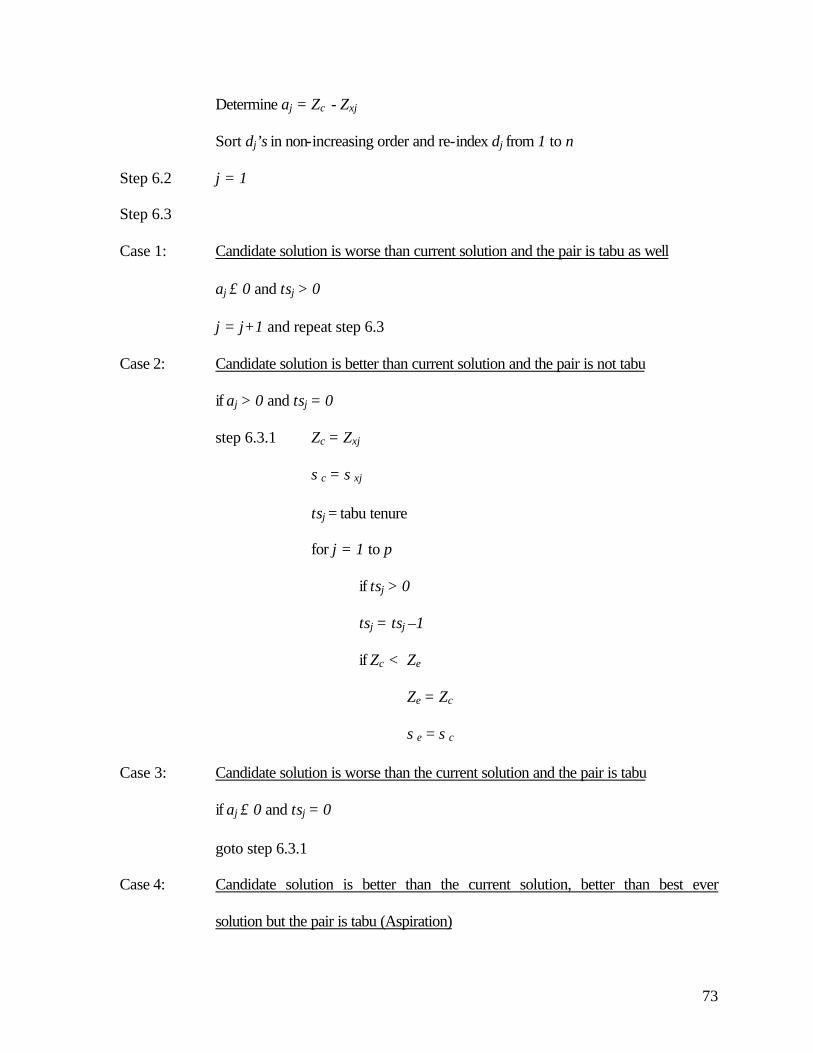
73
Determine aj = Zc - Zxj
Sort dj’s in non-increasing order and re-index dj from 1 to n
Step 6.2 j = 1
Step 6.3
Case 1: Candidate solution is worse than current solution and the pair is tabu as well
aj ≤ 0 and tsj > 0
j = j+1 and repeat step 6.3
Case 2: Candidate solution is better than current solution and the pair is not tabu
if aj > 0 and tsj = 0
step 6.3.1 Zc = Zxj
σc = σxj
tsj = tabu tenure
for j = 1 to p
if tsj > 0
tsj = tsj –1
if Zc < Ze
Ze = Zc
σe = σc
Case 3: Candidate solution is worse than the current solution and the pair is tabu
if aj ≤ 0 and tsj = 0
goto step 6.3.1
Case 4: Candidate solution is better than the current solution, better than best ever
solution but the pair is tabu (Aspiration)

74
if aj > 0 and tsj > 0 and Ze > dj
goto step 6.3.1
Step 6.4 If i = t, STOP, else i = i + 1 and goto Step 6.1.1.
Step 2.1 determines the release dates and due dates at the bottleneck machine for all jobs.
Step 2.2 determines the priority of a job that is yet to be selected in a partial sequence. The
job with the highest priority is selected and appended to the partial sequence in step 2.3.
Schedule of the partial sequence is developed in step 2.4. In step 2.5, based on the
completion time of the last job of the partial sequence at the bottleneck machine, release
dates of the jobs not in the partial sequence are updated. Similarly, in step 2.6, due dates of
the jobs not in the partial sequence at the bottleneck stage are determined. In step 2.7, a
complete permutation flowshop sequence is determined. In step 3, we shift jobs that
complete before the due date and have idle times at the last machine towards the due date.
This reduces the earliness costs while maintaining the feasibility of the schedule. In step 4 we
reduce the earliness and tardiness costs by increasing the completion time of jobs at the last
machine as long as the number of early jobs are more than the number of on-time jobs and
tardy jobs. Step 5 determines the objective value of the schedule.
In step 6 we apply tabu search, a local neighbor hood search procedure to improve the
value of objective function. In tabu search procedure, parameters are the number of tabu
iterations and the tabu tenure. Tabu iterations are the number of iterations over which the
tabu procedure is applied. In this procedure, typical tabu iteration would have following
steps. From the n jobs, p = n(n-1)/2 pairs are created. From the current sequence derived
after step 5, p candidate sequences are obtained by applying pair wise interchange at the
current sequence. All p sequences are scheduled based on the steps described in heuristic and
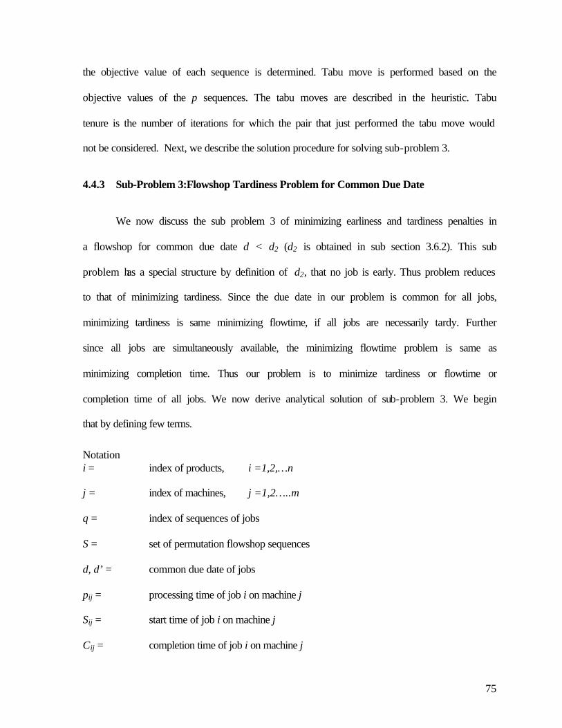
75
the objective value of each sequence is determined. Tabu move is performed based on the
objective values of the p sequences. The tabu moves are described in the heuristic. Tabu
tenure is the number of iterations for which the pair that just performed the tabu move would
not be considered. Next, we describe the solution procedure for solving sub-problem 3.
4.4.3 Sub-Problem 3:Flowshop Tardiness Problem for Common Due Date
We now discuss the sub problem 3 of minimizing earliness and tardiness penalties in
a flowshop for common due date d < d2 (d2 is obtained in sub section 3.6.2). This sub
problem has a special structure by definition of d2, that no job is early. Thus problem reduces
to that of minimizing tardiness. Since the due date in our problem is common for all jobs,
minimizing tardiness is same minimizing flowtime, if all jobs are necessarily tardy. Further
since all jobs are simultaneously available, the minimizing flowtime problem is same as
minimizing completion time. Thus our problem is to minimize tardiness or flowtime or
completion time of all jobs. We now derive analytical solution of sub-problem 3. We begin
that by defining few terms.
Notation i = index of products, i =1,2,…n
j = index of machines, j =1,2…..m
q = index of sequences of jobs
S = set of permutation flowshop sequences
d, d’ = common due date of jobs
pij = processing time of job i on machine j
Sij = start time of job i on machine j
Cij = completion time of job i on machine j
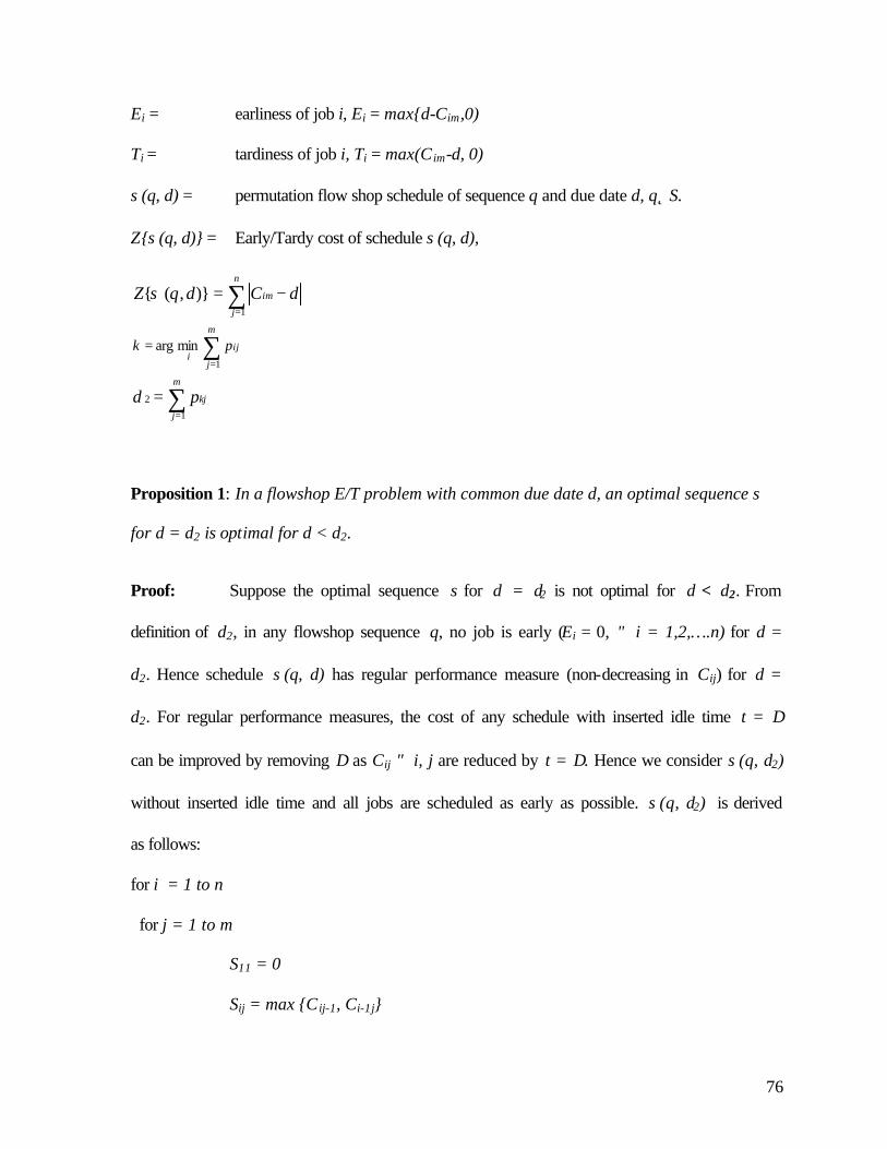
76
Ei = earliness of job i, Ei = max{d-Cim,0)
Ti = tardiness of job i, Ti = max(C im-d, 0)
σ(q, d) = permutation flow shop schedule of sequence q and due date d, q∈S.
Ζ{σ(q, d)} = Early/Tardy cost of schedule σ(q, d),
∑=
−=n
j
im dCdqZ1
)},({σ
∑=
=m
j
iji
pk1
minarg
∑=
=m
j
kjpd1
2
Proposition 1: In a flowshop E/T problem with common due date d, an optimal sequence s
for d = d2 is optimal for d < d2.
Proof: Suppose the optimal sequence s for d = d2 is not optimal for d < d2. From
definition of d2, in any flowshop sequence q, no job is early (Ei = 0, ∀ i = 1,2,….n) for d =
d2. Hence schedule σ(q, d) has regular performance measure (non-decreasing in Cij) for d =
d2. For regular performance measures, the cost of any schedule with inserted idle time t = ∆
can be improved by removing ∆ as Cij ∀ i, j are reduced by t = ∆. Hence we consider σ(q, d2)
without inserted idle time and all jobs are scheduled as early as possible. σ(q, d2) is derived
as follows:
for i = 1 to n
for j = 1 to m
S11 = 0
Sij = max {C ij-1, Ci-1j}

77
Cij = Sij + pij
∑=
−=n
j
im dCdqZ1
22)},({σ
From definition of Z{σ(q, d2)}, it can be seen that:
for d = d2-1, Z{σ(q, d)} increases by n,
for d = d2-2, Z{σ(q, d)} increases by 2n,
for d = d2-x, Z{σ(q, d)} increases by xn.
Thus for any d < d2, Z{σ(q, d)} increases by (d2-d)n,
Hence for d < d2, Z{σ(q, d)} = Z{σ(q, d2)}+ (d2-d)n
Now consider an optimal sequence s for d = d2. Suppose s is not optimal for a due date d’
where d’ < d2. Consider another sequence s1, which is optimal for d’ < d2. Then we have,
Ζ{σ(s, d’)}= Ζ{σ(s, d2)}+ (d2-d’) n (1)
Ζ{σ(s1, d’)}= Ζ{σ(s1, d2)}+ (d2-d’) n (2)
If s is not optimal for d’,
Ζ{σ(s, d’)}> Ζ{σ(s1, d’)} (3)
From (1), (2) and (3) ,
Ζ{σ(s, d2)}+ (d2-d’)n > Ζ{σ(s1, d2)}+ (d2-d’)n
Thus, Ζ{σ(s, d2)}> Ζ{σ(s1, d2)}. This is a contradiction as s is an optimal sequence for d =
d2. Hence s is an optimal sequence for d < d2.
Q.E.D. This result has implications that the optimal solution of flowshop tardiness problem
for common due date d ≤ d2 (sub-problem 3) remains same for range of d. It is, however,

78
difficult to analytically obtain the optimal solution of sub-problem 3. We develop heuristic
algorithm for the problem. Several researchers have investigated the problem of minimizing
tardiness, flowtime, and completion time in permutation flowshops. The equivalence of these
three objectives was shown above. We have compared the performance of our heuristic with
the existing results and found our proposed heuristic to perform better.
The concept used in the heuristic is same used in heuristic algorithm of sub-problem
2. We derive permutation flowshop sequence at the bottleneck machine. The one minor
difference between the heuristics of sub problems 2 and 3 is that the priority function of a job
is determined differently. This is because in sub-problem 3 we are solving n/1/ri/ΣTi,
whereas in sub-problem 2 we are solving n/1/ri/ΣEi +Ti. Secondly, the steps of improving
earliness and tardiness costs of heuristic of sub-problem 2 are not required. The steps of the
heuristic solution of sub-problem 3 are explained below.
4.4.3.1 Heuristic Algorithm (H2) for Sub-Problem 3
Heuristic H2 for Solving Sub-Problem 3
Steps 1 to steps 2.1 are same as in heuristic for solving sub-problem 2.
Step 2.2 Determining priority ui of jobs
ui = max(rik, t) + max{max(rik, t) + pik, dik}
where t = current time = Cσk
Step 2.3 to step 2.7 are same as in heuristic for sub-problem 2.
Steps 3 and steps 4 are not required as no job is early.
Steps 5 and steps 6 are same as in heuristic for sub-problem 2.

79
Next, we describe the solution procedure for solving the intermediate products scheduling
problem.
4.5 Solution Procedure for Intermediate Products Scheduling Model
In this section, we develop the solution procedure for the intermediate products
scheduling problem. The main difference between finished goods and intermediate products
is in the production process. While the production process of finished goods resemble
flowshop pattern, intermediate products are processed in a general jobshop pattern with re-
entrant flows. This means that intermediate products do not have similar routes in the
production process. This increases the complexity of scheduling in the flexible plant. One
important consideration in the intermediate products scheduling is that there cannot be any
tardiness in the schedule. This is because, intermediate products derive their due date from
the schedule of higher-level products as seen in chapter 1. Based on the product structure,
higher-level products are scheduled first, their schedule is translated in the requirements (due
dates) of their lower level intermediate products. To maintain feasibility of the schedule of
product structure, products at any level (except level 0 products, which are finished goods)
cannot be tardy. Hence only earliness costs need to be minimized in the intermediate
products scheduling problem. We have developed the solution algorithm for intermediate
products on these lines. We describe the heuristic now to determine intermediate products
schedule.
As discussed in section 4.4, we are minimizing earliness in the intermediate product
scheduling, tardiness has to be zero to maintain feasibility of the schedule. At a particular
level of product structure, we sort all jobs of the level on the basis of their due dates. Jobs
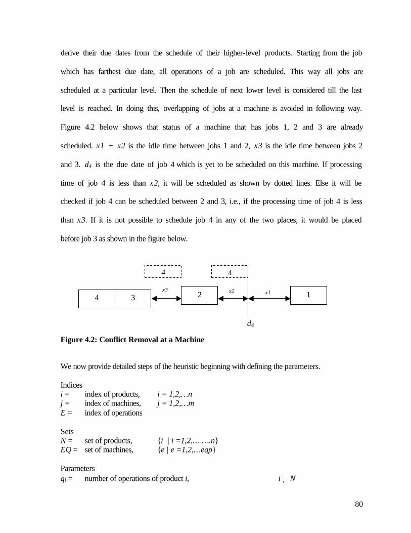
80
derive their due dates from the schedule of their higher-level products. Starting from the job
which has farthest due date, all operations of a job are scheduled. This way all jobs are
scheduled at a particular level. Then the schedule of next lower level is considered till the last
level is reached. In doing this, overlapping of jobs at a machine is avoided in following way.
Figure 4.2 below shows that status of a machine that has jobs 1, 2 and 3 are already
scheduled. x1 + x2 is the idle time between jobs 1 and 2, x3 is the idle time between jobs 2
and 3. d4 is the due date of job 4 which is yet to be scheduled on this machine. If processing
time of job 4 is less than x2, it will be scheduled as shown by dotted lines. Else it will be
checked if job 4 can be scheduled between 2 and 3, i.e., if the processing time of job 4 is less
than x3. If it is not possible to schedule job 4 in any of the two places, it would be placed
before job 3 as shown in the figure below.
Figure 4.2: Conflict Removal at a Machine
We now provide detailed steps of the heuristic beginning with defining the parameters.
Indices i = index of products, i = 1,2,…n j = index of machines, j = 1,2,…m E = index of operations Sets N = set of products, {i | i =1,2,… ….n} EQ = set of machines, {e | e =1,2,…eqp} Parameters qi = number of operations of product i, i ∈ N
2 1
d4
x3 x1 x2
4 4
4 3

81
pij = processing time of product i on machine j, i ∈ N eij = machine used by product i at machine j, i ∈ N Xi = quantity (in units) of product i to be produced i ∈ N
as proposed by planning model Ii = inventory (in units) of product i at the beginning i ∈ N
of the scheduling period Bi = standard batch size (in units) of product i, i ∈ N mi = number of batches between two setups for product i, i ∈ N Mi = setup time (in hours) of product i, i ∈ N rik = amount of i (in units) in one batch of product k, i, k ∈ N Pi = set of products for which i is an input, {k | rik>0}, i, k ∈ N Di = number of due dates of product i, i ∈ N dix = xth due date of product i, i ∈ N, x =1,2,…Di Rix = Requirement of product i in xth due date, i ∈ N, x =1,2,…Di
tix = time of xth due date of product i at level 0, i=1,2,3…..n0, x =1,2,…Di
Aix = Production quantity of product i in xth due date, i ∈ N, x =1,2,…Di
nix = number of batches of product i in xth due date, i ∈ N, x =1,2,…Di inti = number of intermediates of product i, i ∈ N L = number of levels in the product structure i, i ∈ N Sabxi = start time of ath batch of bth stage in xth due date of product i,
i ∈ N, x =1,2…Di, b=1,2…qi, a=1,2,…nix. Cabxi = completion time of ath batch of bth stage in xth due date of product i,
i ∈ N, x=1,2…Di, b=1,2…qi, a=1,2,…nix. ce = number of machines scheduled on machine e, e ∈ EQ e1ec = time (in hours) from which machine e available y =1,2,..ce+1,
e ∈ EQ at yth count, e2ec = time (in hours) for which machine e is available from ef1ec at yth count,
y =1,2…, ce+1, e ∈ EQ nll = number of products at level l, l = 1,2,…L. SDl = sorted values of products and their due dates in l =1,2,…L.
non-increasing order of due dates at level l,
Step 1 Determining production quantities after netting out inventory at all levels
for l = 1 to L
for i = 1 to nll
for x =1 to Di
Step 1.1
−−= ∑ ∑=
−
=
x
k
x
k
ikiikix AIRA1
1
1
0 ,max
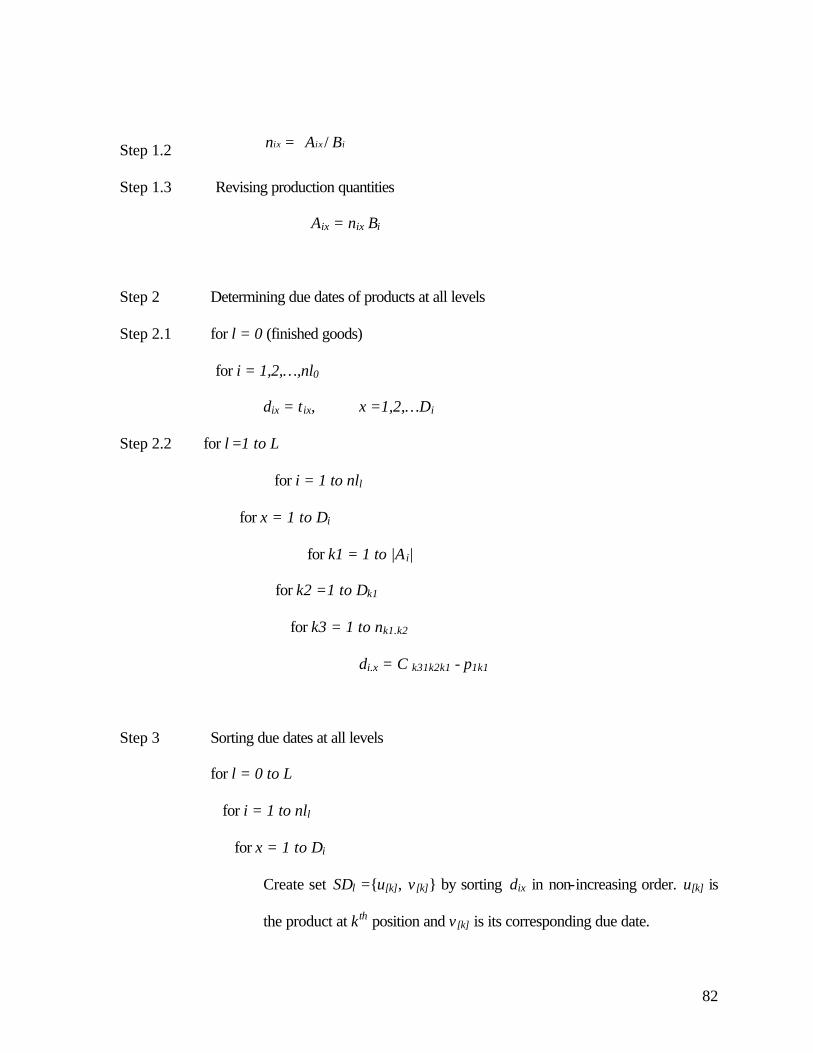
82
Step 1.2 iixix BAn /=
Step 1.3 Revising production quantities
Aix = nix Bi
Step 2 Determining due dates of products at all levels
Step 2.1 for l = 0 (finished goods)
for i = 1,2,…,nl0
dix = tix, x =1,2,…Di
Step 2.2 for l =1 to L
for i = 1 to nll
for x = 1 to Di
for k1 = 1 to |A i|
for k2 =1 to Dk1
for k3 = 1 to nk1.k2
di.x = C k31k2k1 - p1k1
Step 3 Sorting due dates at all levels
for l = 0 to L
for i = 1 to nll
for x = 1 to Di
Create set SDl ={u[k], v[k]} by sorting dix in non-increasing order. u[k] is
the product at kth position and v[k] is its corresponding due date.

83
∑∑= =
=l inl
i
D
x
ixn1 1
lSD , k = 1 to |SDl| ,
Step 4 Schedule level 0 products (finished goods) through solution procedure
described in section 4.3 of this chapter.
Step 5 Scheduling the products at all levels from 1 to L
for l = 1 to L
Step 5.1 Schedule the products at all machines
for j = 1 to |SDl|
i = u[j], u[j] ∈ SDl
x = v [j], v[j] ∈ SDl
a = nix,
Step 5.2 Schedule starting from the last operation
b = qi ,
e = eqib,
ce =0,
for k = 1 to ce + 1
Step 5.2.1 Conflict checking
if (ec = 0)
Cabxi = dix
if (n = r m + 1)
Sabxi = Cabxi – n piq - Mi
else
Sabxi = Cabxi – n piq
else
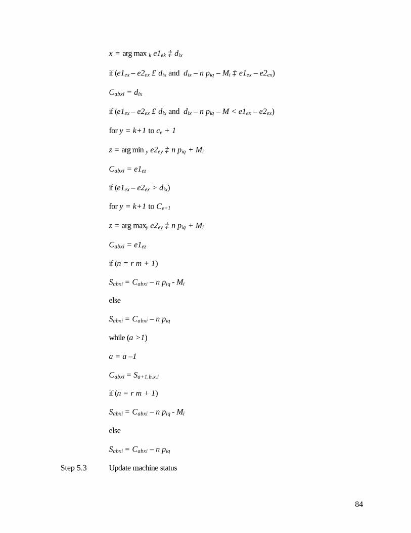
84
x = arg max k e1ek ≥ dix
if (e1ex – e2ex ≤ dix and dix – n piq – Mi ≥ e1ex – e2ex)
Cabxi = dix
if (e1ex – e2ex ≤ dix and dix – n piq – M < e1ex – e2ex)
for y = k+1 to ce + 1
z = arg min y e2ey ≥ n piq + Mi
Cabxi = e1ez
if (e1ex – e2ex > dix)
for y = k+1 to Ce+1
z = arg maxy e2ey ≥ n piq + Mi
Cabxi = e1ez
if (n = r m + 1)
Sabxi = Cabxi – n piq - Mi
else
Sabxi = Cabxi – n piq
while (a >1)
a = a –1
Cabxi = Sa+1.b.x.i
if (n = r m + 1)
Sabxi = Cabxi – n piq - Mi
else
Sabxi = Cabxi – n piq
Step 5.3 Update machine status
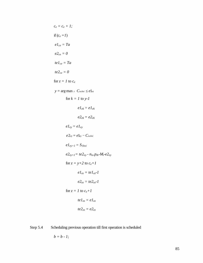
85
ce = ce + 1;
if (ce =1)
e1ce = Ta
e2ce = 0
te1ce = Ta
te2ce = 0
for z = 1 to ce
ezbxin z eC y ix 1maxarg ≤=
for k = 1 to y-1
e1ek = e1ek
e2ek = e2ek
e1ey = e1ey
bxineyey ixCee −= 12
e1ey+1 = S1bxi
e2ey+1= te2ey - nix.pib-Mi-e2ey
for z = y+2 to ce+1
e1ez = te1ez-1
e2ez = te2ez-1
for z = 1 to ce+1
te1ez = e1ez
te2ez = e2ez
Step 5.4 Scheduling previous operation till first operation is scheduled
b = b - 1;

86
while (qi >1)
e = eqib,
a = nix,
if (pib ≤ pib+1)
{ } ibib ibixxibnbxin pppnCC xx ++−+ −= )( 11
if (pib > pib+1)
11 +−+= ibxibnxin pCC ixixb
Go to step 5.3
If b = 1, STOP, else repeat Step 5.4.
Step 1 determines the number of batches of each product in one production run. The
importance of this step is that it makes use of the available inventory while scheduling a
product. A finished good could have many due dates, i.e., several customer orders. Orders
that are in beginning of the scheduling period may be fulfilled from the inventory. However,
if the entire quantity proposed by the production-planning model has to be scheduled, the
availability of inventory gives the scheduler some degree of flexibility. In step 2.1, the due
dates of finished good are specified. These are based on the customer orders. Finished goods
have several due dates (customer orders). In step 2.2, we determine the due dates of
intermediate products. At the time of determining due date of an intermediate product at a
particular level, its higher-level product (where the intermediate product is input) is already
scheduled. Based on this schedule, the due date of an intermediate product is determined. As
in the case of finished goods, intermediate products would also have several due dates
depending on how many times an intermediate product is required. In step 3, due dates are
sorted in non-increasing order. Step 4 schedules the finished products according to the

87
solution procedure described in section 4.3 of this chapter. We have to apply this procedure
as many times as there are due dates of finished goods. Scheduling problem is decomposed
into as many problems as there are common due dates in the scheduling horizon. In step 5,
we schedule the intermediate products at all levels starting from level 1. The products are
selected on the basis of sorted due dates at a level and beginning from the last operation, all
operations of a product are scheduled till first operation is scheduled. It is ensured in step 5.2
that there is no overlapping of products on a machine. The explanation of this step is also
provided in sub-section 4.4.1. In step 5.3, after any operation is scheduled on a machine, the
availability status of the machine is updated. Step 5.4 ensures that all operations of a product
are scheduled. In the next section, we describe the solution procedure for solving dedicated
plants scheduling problem.
4.6 Dedicated Plant Scheduling Heuristic
There are some production plants in the production environment that produce only
one type of product. These are called as dedicated production plants. We develop heuristic
algorithm to schedule the products on dedicated production plants. The procedure is
explained below.
Parameters
N = number of batches to be produced
q = index of machines, q = 1, 2, 3, …..k,…..K
nq = number of machines in machine q
pq = processing time of machine q
e = index of machines, e = 1,2,…..,E

88
m = number of batches after which set-up is required
M = set-up time (in hours)
Ta = time available in a scheduling period
Sqne = start time of qth machine of nth batch on machine e
Cqne = completion time of qth machine of nth batch on machine e
Dedicated Plant Scheduling Procedure (H3)
Step 0 Determination of Bottleneck Operation
Let ‘k’ be the bottleneck operation
1 to k-1: Pre-bottleneck operation
k +1 to K: Post-Bottleneck operation
Bottleneck operation capacity:
Step 1 Scheduling Bottleneck Operation
Q = k
N = n
E = 1
Step 1.1
Step 1.2 If n/nk = r m+1 for r = 0,1,2,,,,,N/m
Yesà x = 1
Noà x = 0
Step 1.3 xMpCS kknekne .−−=
[ ] )}./
(/{maxarg Mm
nNnNpk
qqq
q
+=
∑+=
−=K
kq
qakne pTC1

89
Step 1.4 Is n ≤ nk
Yesà Check is e = nk
Yesà STOP
Noà e = e +1
n = n – e + 1
Goto Step 1.2 and get xMpCS kknekne .−−=
Noà n = n-nk
enknkne kSC +=
Check Step 1.2 and get MxpCS kknekne −−=
Goto Step 1.4
Step 2 Scheduling Pre-Bottleneck Operations
q = k – 1
n =N
e =1
Step 2.1 ),min( 11 enqnqneqqne qSpCC +++ −=
Step 2.2 If n/nk = rm+1 for r = 0,1,2,….,N/m
Yesà x = 1
Noà x = 0
Step 2.3 MxpCS qqneqne −−=
Step 2.4 Is n = 1
Yesà Go to Step 2.5
Noà check is e = nq

90
Yesà e = 1
No à e = e + 1
n = n –1
Repeat Step 2.1
Step 2.5 Is q = 1
Yesà STOP
Noà q = q –1
n = N
e = 1
Goto Step 2.1
Step 3.0 Scheduling Post-Bottleneck Operation
q = k + 1
n = 1
e = 1
Step 3.1 qneqqne pCC +−= 1
Step 3.2 If n/nk = rm+1 for r = 0,1,2,,,,,N/m
Yesà x = 1
Noà x = 0
Step 3.3 MxpCS qqneqne −−=
Step 3.4 eqnqne CSd 1−−=
Step 3.5 Is d ≥ 0

91
Yesà Check if n = N
Yesà Goto Step 3.6
Noà Is e = nk
Yesà e = 1
Noà e = e + 1
n = n + 1
Repeat Step 3.1
Noà eqnqne CS 1−=
Check Step 3.2 and get MxpSC qqneqne ++=
Repeat Step 3.4
Step 3.6 Is q ≠ K
Yesà q = q + 1
n = 1
e = 1
Repeat Step 3.1
Noà STOP
Step 0 determines the bottleneck operation in the dedicated production plant. There are
several machines available for an operation. The bottleneck operation is the operation with
maximum sum of processing time and setup time required for a product amongst all
operation. Step 1 schedules the bottleneck operation. Step 2 and step 3 schedule the pre-
bottleneck operations and post-bottleneck operations respectively.

92
4.7 Summary
In this chapter, we developed solution procedures for solving the production planning
and scheduling problem. We use branch and bound algorithm to solve the production-
planning problem. We have two models for scheduling problem, one of the finished good
scheduling problem and the other model of intermediate products scheduling problem. The
finished goods scheduling problem can be decomposed into three sub-problems based on the
value of common due date. The three sub-problems are called as flowshop E/T problems
with unrestricted due date, intermediate due date and restricted due date respectively. Due
date is common for all jobs in all three sub-problems. We derive analytical results and obtain
optimal schedule of sub-problem 1. For sub-problem 2, we develop a heuristic algorithm and
derive permutation flowshop sequence. We derive an analytical result for solving sub-
problem 3 in the restricted due date range. We also propose heuristic algorithm for obtaining
permutation flowshop sequence for sub-problem 3. In the next chapter, we report
computational results of the solution procedure for production planning and scheduling
problem.

93
5 Results of Production Planning and Scheduling Problem
5.1 Introduction
In this chapter, we provide the results of solution procedures used for solving the
production planning and scheduling problem. We also report the sensitivity analysis on the
results. The data for studying the results of production planning and scheduling problem, is
provided by a pharmaceutical company in India.
The solution procedures for production planning and scheduling problems were
described in chapter 4. We solve the production-planning problem using the branch and
bound algorithm from a commercial solver. We develop analytical results for sub-problem 1
of finished goods scheduling problem. Before applying the solution procedure to the overall
production planning and scheduling problem, we test the performance of heuristic algorithms
for solving sub-problems 2 and 3 on some benchmark problems in literature on flowshop
scheduling.
The rest of this chapter is organized as follows. We have the optimal solution for sub-
problem 1 in chapter 4. In the next section, we describe the experiment design and lower
bound of sub-problem 2, and computational performance of heuristic algorithms for solving
sub-problem 2. In section 5.3, we discuss the lower bound of sub-problems 3, some of the
existing heuristic algorithms for solving sub-problem 3 and computational performance of
the proposed heuristics for solving sub-problem 3. In section 5.4, we study the results of
production planning and scheduling problem. The summary of this chapter is provided in
section 5.6. We begin by studying the results of sub-problem 2 in the next section.

94
5.2 Results of Sub Problem 2
Sub-problem 2 is the flowshop E/T problem with intermediate common due date, i.e.,
problems where the due date falls in between restricted and unrestricted due dates for
flowshop problems. In this section, we describe a valid lower bound of sub-problem 2. We
also describe the experiment design to test the computation performance of the heuristic.
Subsequently, we discuss the results of the solution procedure for sub-problem 2.
5.2.1 Lower Bound of Sub Problem 2
In this section, we develop the lower bound of sub-problem 2. Our objective is to get
a valid lower bound of a job on its earliness and tardiness. We begin with some definitions.
Notation i = index of jobs, i =1,2,…n. j = index of machines, j =1,2…..m. d = common due date of all jobs pij = processing time of job i on machine j Oj(i) = sum of i shortest processing times on machine j amongst all jobs LBCi = lower bound on the completion time of job i on machine m. Cim = completion time of job i on machine m LBETi = lower bound on earliness and tardiness of job i
In a permutation flowshop, the completion time of the ith job on the last stage m, i.e.,
(LBCi) of any sequence is not less than
−+ ∑=
≤≤
m
l
ijiilijmj ppiO1
1 minmin)(max . Oj(i) is a
lower bound on the time needed to process i jobs on machine j. Therefore, Cim is not less than
the sum of Oj(i) and the minimum processing times among all jobs on machine 1 through m
except machine j. Since this is true for all machines, the LBCi is a valid lower bound on
completion time of ith job on last machine of any sequence. LBCi is provided by Kim (1995).
The lower bound on earliness and tardiness of job i is given by: LBETi = max{d - LBCi, 0} +
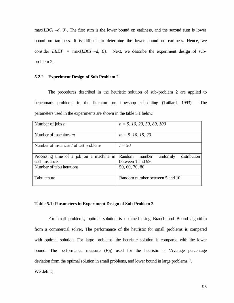
95
max{LBCi –d, 0}. The first sum is the lower bound on earliness, and the second sum is lower
bound on tardiness. It is difficult to determine the lower bound on earliness. Hence, we
consider LBETi = max{LBCi –d, 0}. Next, we describe the experiment design of sub-
problem 2.
5.2.2 Experiment Design of Sub Problem 2
The procedures described in the heuristic solution of sub-problem 2 are applied to
benchmark problems in the literature on flowshop scheduling (Taillard, 1993). The
parameters used in the experiments are shown in the table 5.1 below.
Number of jobs n n = 5, 10, 20, 50, 80, 100
Number of machines m m = 5, 10, 15, 20
Number of instances I of test problems I = 50
Processing time of a job on a machine in each instance.
Random number uniformly distribution between 1 and 99.
Number of tabu iterations 50, 60, 70, 80
Tabu tenure Random number between 5 and 10
Table 5.1: Parameters in Experiment Design of Sub-Problem 2
For small problems, optimal solution is obtained using Branch and Bound algorithm
from a commercial solver. The performance of the heuristic for small problems is compared
with optimal solution. For large problems, the heuristic solution is compared with the lower
bound. The performance measure (PH) used for the heuristic is ‘Average percentage
deviation from the optimal solution in small problems, and lower bound in large problems. ’.
We define,
96
ZHI: Objective value of heuristic solution of instance I
ZOI: Objective value of optimal solution of instance I
ZLBI: Lower bound of the instance I
For smaller problems (n =5, 10; m =5)
1001
−= ∑
I OI
OIHIH
ZZZ
IP
For large problems (n > 10)
1001
−= ∑
I LBI
LBIHIH
ZZZ
IP
LBCi is a weak lower bound (Kim, 1995). As mentioned above, it is difficult to
estimate the lower bound on earliness. Thus, LBETi is a very weak lower bound on earliness
and tardiness. This is verified for small problems (n = 5, 10; m =5), as the average
percentage deviation of optimal solution from the lower bound is found to very high. In case
of n = 5;m = 5; 50 instances, average percentage deviation of optimal solution from lower
bound is 326 percent and in case of n = 10; m = 5, it is found to be 284 percent. The average
percentage deviation of heuristic solution from lower bound for small and large problems for
5-machines problem is shown in figure 5.1 and for 10-machines problem in figure 5.2. The
deviation is again high but this is expected, as the deviation of lower bound is high from
optimal solution itself. Since both heuristic solution and optimal solution deviate by almost
same percentage from the lower bound for smaller problems, it is obvious that, at least for
small problems, heuristic solution and optimal solution are close to each other. For (n = 5,
10; m =5), the average percentage deviation of optimal solution from heuristic solution is
0.894 percent and 1.126 percent for 5 jobs and 10 jobs respectively. The common due date

97
considered for this analysis is d = (d1+d2)/2. The observations are encouraging for
measuring heuristic performance, as the optimal solution also has large deviation from the
lower bound.
Figure 5.1: Average % Deviation of Heuristic Solution from Lower Bound: 5 Machines
The performance of the heuristic for smaller problems is also compared with optimal
solution with a random common due date between d1 and d2. This is done to evaluate the
quality of heuristic solution in the entire range of intermediate due date. The results of n =
5;m = 5; 50 instances with random due date between d1 and d2 were 0.846 percent average
deviation of heuristic solution from the optimal solution. For of n = 10;m = 5; 50 instances,
the average deviation of heuristic solution from the optimal solution is 1.247 percent.
Average % Deviation from Lower Bound
050
100150200250300350
5 10 20 50 80 100
Jobs
% D
evia
tio
n

98
Figure 5.2: Average of Deviation of Heuristic Solution from Lower Bound: 10 Machines
As discussed above that the lower bound of sub-problem 2 is very weak, the performance
measure of the heuristic for larger problems is tested for common due date value d1(obtained
in sub problem 1). This is because we have optimal solution of flowshop E/T problem for
common due date d1, obtainable in polynomial time. The results of this comparison are
indicated in table 5.2. The results in table 5.2 indicate the average percentage deviation of
optimal solution at d = d1 from the heuristic solution. Each job and machine combination
discussed in the experiment design is shown in table 5.2. The results of table 5.2 indicate that
the performance of heuristic H1 is good, as the maximum average percent deviation of the
optimal solution from lower bound is found to be 1.744 percent. The results in table 5.2
indicate that the average percentage deviation of jobs for a particular machine follow a non-
linear pattern. This is indicated for 5-machine problem in figure 5.3. The non-linear pattern is
observed for m = 10, 15 and 20 also.
Average % Deviation from Lower Bound
0100200300400500600
5 10 20 50 80 100
Jobs
% D
evia
tio
n

99
Machines
Jobs 5 10 15 20
5 0.000 0.000 0.235 0.000
10 0.084 0.081 0.099 0.276
20 0.074 0.020 0.012 0.023
50 0.323 0.153 0.152 0.146
80 0.865 0.642 0.617 0.644
100 1.744 1.168 1.175 1.129
Table 5.2: Average Percentage of Deviation of Optimal Solution from Heuristic
Solution
As it is seen in the figure 5.3, with increase in the number of jobs, the average percentage
deviation follows a square ordered pattern. The square root of the average percentage
deviation follows a linear pattern. These results are with 50 tabu iterations in each of the 50
instances solved for a particular job-machine combination
0.00.51.01.52.0
10 20 50 80 100
Number of Jobs
Average % Deviation Square Root of Average % Deviation
Figure 5.3: Average % Deviation from Optimal Solution and its Square Root

100
When number of tabu iterations is increased, the results improve as the average percentage
deviation is reducing. This however, would increase the computational time to solve the
problem. The improvement in results with increase in number of tabu iterations is shown in
figure 5.4 for n = 50, m = 5. As seen in figure 5.4, the solution at 100 tabu iterations is
around 70 percent better than the solution at 50 tabu iterations.
Figure 5.4: Improvement in the solution with Increase in Number of Tabu Iterations
5-machine case is analyzed in detail to observe the pattern of the results. At 100 tabu
iterations, the average percentage deviation follows an almost linear pattern as compared to
50-tabu iterations. This phenomenon is shown in figure 5.5. The figure indicates for m = 5,
and n = 5, 10, 20, 50, 80 and 100, the average percentage deviation of heuristic solution from
optimal solution for 50 and 100 tabu iterations. In the next section, we discuss the results of
sub problem 3.
0.000.050.100.150.200.250.300.35
50 60 70 80 90 100
Tabu Iterations
% D
evia
tion

101
Figure 5.5: Comparison of Results with Different Tabu Iterations
5.3 Results of Sub Problem 3
In this section, we discuss the results of flowshop E/T problem with restricted
common due date, i.e., d < d2. The special structure of sub-problem 3 was discussed in
chapter 4. The objective of this problem is to minimize earliness and tardiness. Because of
the common due date and the property that no job is early, the objective of the problem is
same as that of minimizing flowtime and minimizing completion time. As a result, we use
one of the better-known lower bounds in literature, of flowshop completion time problem, as
the lower bound of sub-problem 3. Lower bound of flowshop completion time problem is
due to Ahmadi and Bagchi (1990). We describe this lower bound in the next sub-section.
00.20.40.60.8
11.21.41.61.8
2
5 10 20 50 80 100
Jobs
Ave
rag
e %
Dev
iati
on
100 iterations 50 iterations

102
5.3.1 Lower Bound of Sub Problem 3 (Ahmadi and Bagchi, 1990)
Notation N = set of n jobs, {i | i = 1,2, …,n} . M = set of m machines in a flowshop, {j | j = 1,2,…, m} pij = processing time of job i on machine j π = set of r jobs constituting a partial schedule which specifies
completion times of the jobs in π on all machines π’ = set of n-r jobs such that π’r = N - πr Cπ.j = completion time of the partial schedule π on machine j, or the
earliest time machine j is available for processing a job in π’ Cij = completion time of job i on machine j σ = a complete sequence of n jobs Cσ = sum of completion times on last machine m of all jobs in σ
Cσ can be written as:
'
∑ ∑∈ ∈
+=π π
σ
i i
imim CCC (1)
The first sum on the right hand side in (1) is a constant. The optimal value of the
second sum is the solution to the following mathematical programming problem P1 where
the minimization is taken over V, the set of all possible sequences of the jobs in π’:
Let Ci0 = 0 for all i∈ N, and [i] is the job in the ith position in a sequence, and C[0].j = 0 for all
j∈ M.
Problem P1 ∑∈ '
minπi
imV
C
s.t. Cij ≥ Cπj + pij, i∈π’, j∈ M (2)
Cij ≥ Cij-1 + pij, i∈π’, j∈ M (3)
C[i]j ≥ C[i-1]j + p[i]j, i=r+1, r+2,…,n, j∈ M (4)
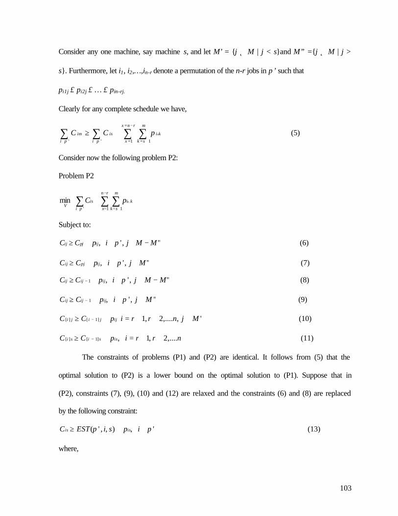
103
Consider any one machine, say machine s, and let M’ = {j ∈ M | j < s}and M” ={j ∈ M | j >
s}. Furthermore, let i1, i2,…,in-r denote a permutation of the n-r jobs in π’ such that
pi1j ≤ pi2j ≤ … ≤ pin-rj.
Clearly for any complete schedule we have,
(5) 1 1' '
∑ ∑∑ ∑−=
= +=∈ ∈
+≥rnx
x
m
sk
ki
i i
isim xpCCπ π
Consider now the following problem P2:
Problem P2
min1 1'
.∑ ∑∑−
= +=∈
+rn
x
m
sk
ki
i
isV
xpCπ
Subject to:
(6) " ,' , MMjipCC ijjij −∈∈+≥ ππ
(8) " ,' ,1 MMjipCC ijijij −∈∈+≥ − π
(9) " ,' ,1 MjipCC ijijij ∈∈+≥ − π
(10) ' ,,....2,1 ]1[][ MjnrripCC ijjiji ∈++=+≥ −
(11) ,....2,1 , ]1[][ nrripCC issisi ++=+≥ −
The constraints of problems (P1) and (P2) are identical. It follows from (5) that the
optimal solution to (P2) is a lower bound on the optimal solution to (P1). Suppose that in
(P2), constraints (7), (9), (10) and (12) are relaxed and the constraints (6) and (8) are replaced
by the following constraint:
(13) ' ,),,'( ππ ∈+≥ ipsiESTC isis
where,
(7) " ,' , MjipCC ijjij ∈∈+≥ ππ

104
(14) max,max),,'(1
11
+= ∑−=
=−≤≤
sx
kx
ixksk
s pCCsiEST πππ
The resulting problem P3 is:
(15) min1 1'
. .∑ ∑∑−
= +=∈
+rn
x
m
sk
ki
i
siV
xpCπ
subject to (11) and (13).
Clearly, the optimal solution to (P3) is a lower bound on (P2). Problem (P3) is NP-
Hard and is single machine problem of minimizing the sum of completion times subject to
release times. The second sum in the objective function of (P3) is a constant, and the release
time of job i ∈ π’ is given by EST(π’, i, j). If pre-emption is allowed, (P3) can be optimally
solved by the shortest remaining processing time (SRPT) rule.
Let the objective value of P3 with SRPT schedule be zs. It follows that zs is a lower
bound on problems P3, P2 and P1. The overall lower bound on P1 is: max(z1, z2 , ………zm).
5.3.2 Existing Results of Sub Problem 3
There are several results in the literature on flowshop problems with an objective of
minimizing tardiness, flowtime or completion time of jobs. We apply the best results of these
problems on the instances generated from our experiment design, and compare the solution
of the existing heuristics with our heuristic. We consider following three heuristics existing
in the literature:
105
1. NEH Nawaz et al. (1983)
2. RZ Rajendran and Ziegler (1997)
3. WY Woo and Yim (1998)
We determine average percentage deviation from lower bound on each of the three
heuristics. On the same instances we test our heuristic (H2), which was described in chapter
4. We also propose two more heuristics by applying tabu search procedure on heuristics RZ
and WY. These heuristics are RZT and WYT. Heuristic NEH is not considered for tabu
search, as its performance was worse than other existing heuristics. Figures 5.6 to 5.9 below
shows the comparison of performance measure of existing heuristics and the proposed
heuristics for various jobs and machine combinations.
Figure 5.6 indicates the comparison of three existing heuristics and three new
heuristics developed to solve sub-problem 3. As seen in figure 5.6, the average percentage
deviation of heuristic solution is compared for jobs (n = 5, 10, 20, 50, 80, 100) and 5
machines. Similar jobs are considered for m = 10, m = 15 and m = 20 in subsequent figures.
The average percentage deviation of heuristic solution from lower bound for all jobs is
minimum in H2, the heuristic we developed in chapter 4. For higher number of machines
also (figures 5.7 to 5.9), it is seen that H2 is performing better. In all the heuristics, the
average percentage deviation from lower bound increases with the number of jobs.
It is seen in all the cases that heuristic H2 performs better than the existing heuristics.
The average percentage deviation from lower bound is minimum for H2. Other heuristics on
which tabu is performed (WYT, RZT) also perform close to H2. In the next section, we
discuss the results of the production planning and scheduling problem.
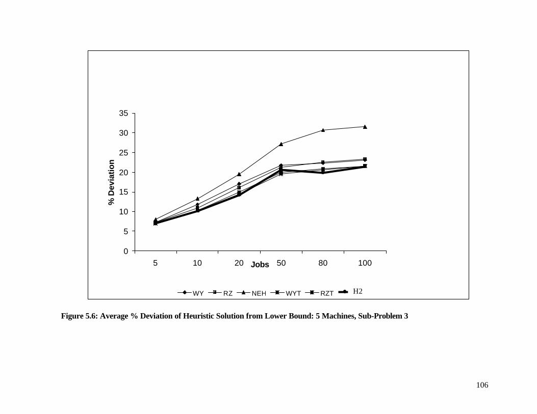
106
0
5
10
15
20
25
30
35
5 10 20 50 80 100Jobs
% D
evia
tio
n
WY RZ NEH WYT RZT H1T
Figure 5.6: Average % Deviation of Heuristic Solution from Lower Bound: 5 Machines, Sub-Problem 3
H2

107
0
5
10
15
20
25
30
35
40
5 10 20 50 80 100Jobs
% D
evia
tio
n
WY RZ NEH WYT RZT H1T
Figure 5.7: Average % Deviation of Heuristic Solution from Lower Bound: 10 Machines, Sub-Problem 3
H2
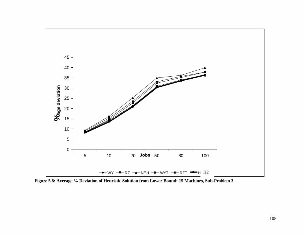
108
0
5
10
15
20
25
30
35
40
45
5 10 20 50 80 100Jobs
%ag
e d
evia
tio
n
WY RZ NEH WYT RZT H1T
Figure 5.8: Average % Deviation of Heuristic Solution from Lower Bound: 15 Machines, Sub-Problem 3
H2

109
Twenty Machine Problem
0
5
10
15
20
25
30
35
40
45
5 10 20 50 80 100Jobs
%ag
e d
evia
tio
n
WY RZ NEH WYT RZT H1T
Figure 5.9: Average % Deviation of Heuristic Solution from Lower Bound: 20 Machines, Sub-Problem 3
H2
110
5.4 Production Planning and Scheduling Results
In this section, we study the results of production planning and scheduling problem.
The data for solving the problem is provided by a pharmaceutical company in India. The
company has multi-stage, multi-product, multi-machine, batch processing environment. The
problem instance solved with 5-month data has 10 finished products, 30 intermediate
products, 50 by-products and 40 reusable raw materials. There are 15 production plants in
this instance. Out of 15 production plants, 8 plants are dedicated production plants and
remaining seven are flexible production plants. In appendix 1, product structure diagram
(panel A) and process flow diagrams (panel B) of each product are shown. The instance
solved is called as the ‘base case’.
The results of the production-planning model are for monthly time period of the 5-
month planning horizon. The decisions obtained are production quantities of finished goods
and intermediate products, number of setups of finished goods and intermediate products,
and inventory levels of finished goods and intermediate products. For illustration, table 5.2
below shows the production quantity of finished goods in each time of the planning horizon.
Column ‘Product’ in table 5.3 indicates the finished goods and column ‘Plant’ indicates the
corresponding production plants of finished goods. Remaining five columns indicate the
production quantities of finished goods in each time period (1,2,…5) of the planning horizon.
Details of the entire production plan and schedule of this base case are provided in appendix
2. For each time period of the planning horizon, appendix 3 consists of production quantities
and number of setups of finished goods and intermediate products (panel A), inventory levels
of finished goods and intermediate products (panel B), capacity utilization of dedicated

111
plants (panel C), capacity utilization of flexible machines (panel D), and schedule of the
plants (panel E). Production planning model gives the total cost of the production plan.
Scheduling results are the start time and completion time of each product on each machine in
each time period of the planning horizon. The overall production planning and scheduling
costs in he instance solved are Rupees 54,127,000.
Time Period
Product Plant 1 2 3 4 5E1 1 13720.00 27000.00 27000.00 27000.00 27000.00
E1 2 0.00 0.00 0.00 0.00 0.00E2 3 1292.13 7000.00 7000.00 7000.00 7000.00E3 4 661.63 2464.93 0.00 2173.44 1820.00
E4 5 0.00 1256.39 4053.26 776.05 1723.95E5 6 1474.15 529.79 1024.50 947.57 0.00E6 7 0.00 0.00 0.00 0.00 740.00
E7 8 2710.00 2200.00 0.00 1785.58 3801.04E7 9 0.00 0.00 7949.42 8200.00 6198.96
E8 10 168.29 556.22 1100.00 1000.00 1000.00
Table 5.3: Production Plan of Finished Goods
We also perform sensitivity analysis on the base case results of production planning
and scheduling problem. We report the results on sensitivity analysis in chapter 6, where we
describe a case study of application of production planning and scheduling models. Next, we
provide summary of this chapter.
5.5 Summary
In this chapter, we discussed the computational performance of the heuristic
algorithms used for solving the production planning and scheduling problem. We discussed
in chapter 4 that the finished goods flowshop E/T problem can be decomposed in three sub-
problems on the basis of common due dates. We have reported optimal solution for flowshop
E/T problem with unrestricted due date (sub-problem 1) in chapter 4. Heuristic algorithms

112
were reported for flowshop E/T problem with intermediate due date (sub-problem 2). We
described the experiment design of testing the computational performance of the heuristic
algorithm in this chapter. We also described a valid lower bound of sub-problem 2 and
discussed the quality of the lower bound. We discussed that the lower bound of sub-problem
2 is very weak. The optimal solution of sub-problem 2 was obtained for small problems (n=5,
10; m=5) using branch and bound algorithm. We tested the computational performance of the
heuristic algorithm for sub-problem 2 by determining the average percentage deviation of
heuristic solution from optimal solution. In small problems, for d = (d1+d2)/2, the average
percentage deviation of heuristic solution from optimal solution is 0.894 percent (n =5, m =
5) and 1.126 percent (n =10, m = 5). For a random due date between d1 and d2, the average
percentage deviation of heuristic solution from optimal solution is 0.846 percent. We also
obtained, for large problems, optimal solution of sub-problem 2 at d = d1, from analytical
results of sub-problem 1. The heuristic of sub-problem 2 is compared with optimal solution
at d = d1. The heuristic solution obtained is very close to the optimal solution at d = d1.
We also developed a valid lower bound for flowshop E/T problem for restricted due
date (sub-problem 3). The computational performance of the proposed heuristic algorithm for
sub-problem 3 was compared with some of the exiting heuristic algorithms of sub-problem 3.
The average percentage deviation of heuristic solution from lower bound is found to be better
in our heuristic as compared to the existing heuristics.
We have reported results of the production planning and scheduling problem. We
studied the production plan of the production planning problem and machine wise schedules
of the scheduling problem. The data for solving the problem is from a pharmaceutical
company in India.
113
In the next chapter, we apply the production planning and scheduling models to a
pharmaceutical company in India. We discuss the results of the solution procedure used to
solve production planning and scheduling problem in this application. We also provide
sensitivity analysis on the results.

114
6 Case Study: Application of Production Planning and Scheduling Models
6.1 Introduction
In this chapter, we apply the production planning and scheduling models developed in
chapter 3 to a real life application. The models are applied to a pharmaceutical company in
India. The company was facing the problem of excess inventories, stockouts and low
capacity utilization in order to meet the demand forecast. Demand fluctuation of the products
was resulting in frequent changes in production plans and schedules on the shop floor. Also
the process to change the products schedule to satisfy changing marketing requirements was
time consuming and tedious. We develop a decision support system to solve the production
planning and scheduling problem of this company.
The plan of this chapter is as follows. We briefly describe the production planning
and scheduling problem in this application in section 6.2. We solve the production planning
and scheduling problem in two steps, as discussed earlier in chapter 3. First, we solve the
production-planning problem. The computational results of solving the production-planning
problem are described in section 6.3. In section 6.4, we develop a variant of the production-
planning model with additional market constraints. This model is used for jointly planning
sales and production. We discuss results of sales and production planning model in this
section. In section 6.5, we solve the scheduling problem. We apply the solution procedure of
scheduling problem developed in chapter 4. The results of the application are discussed in
this section. To provide some managerial insights from the application of production
planning and scheduling models, we provide sensitivity analysis on results in section 6.6. We
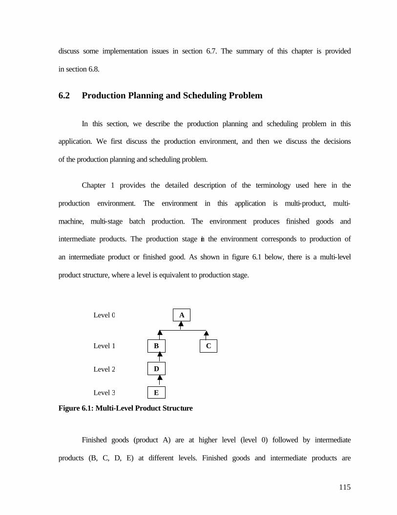
115
discuss some implementation issues in section 6.7. The summary of this chapter is provided
in section 6.8.
6.2 Production Planning and Scheduling Problem
In this section, we describe the production planning and scheduling problem in this
application. We first discuss the production environment, and then we discuss the decisions
of the production planning and scheduling problem.
Chapter 1 provides the detailed description of the terminology used here in the
production environment. The environment in this application is multi-product, multi-
machine, multi-stage batch production. The environment produces finished goods and
intermediate products. The production stage in the environment corresponds to production of
an intermediate product or finished good. As shown in figure 6.1 below, there is a multi-level
product structure, where a level is equivalent to production stage.
Figure 6.1: Multi-Level Product Structure
Finished goods (product A) are at higher level (level 0) followed by intermediate
products (B, C, D, E) at different levels. Finished goods and intermediate products are
A
B C
D
E
Level 0
Level 1
Level 2
Level 3
116
produced in production plants. Each production plant comprises number of machines.
Intermediate products and finished goods are processed on machines in a specific, pre-
determined sequence, called as route. Machines are shared in plants producing intermediate
products and finished goods. There are dedicated plants also in the production process. These
plants produce only one type of product. Intermediate products are stored as work-in-process
inventory.
By-products are generated from intermediate products and finished goods. By-
products are recycled in recycling plants to extract reusable raw materials. The outputs of a
production plant are intermediate products, finished goods and by-products. Inputs to a
production plant are fresh raw materials, reusable raw materials and intermediate products.
Prior to this study, production planning in the company was done on the basis of the
annual demand of the finished goods. Demand is combination of firm orders and forecast.
The production planning method used is similar to the Material Requirements Planning
(MRP) structure. Master schedule for end products is generated first and it is exploded to
determine the intermediate products and raw material requirements A production schedule is
then derived manually based on availability of raw materials and machines, raw material
procurement and manufacturing lead times. Production plans are made with an objective of
maximizing the capacity utilization of machines. This often results in high inventory of
intermediate and end products. The production schedule is forced to undergo frequent
changes due to demand variability, raw materials unavailability, shop-floor uncertainties like
machine breakdowns etc.
117
Production planning and scheduling problem is to determine the decisions at
minimum cost. We developed a decision support system in order to derive production
planning and scheduling decisions and manage the above-mentioned complexities. We have
discussed the production planning and scheduling decisions in detail in chapter 1. We would
briefly revisit them as we are implementing the models in this application. In the next
section, we describe the application of production planning model and its results.
6.3 Application of Production Planning Model
We model the production environment described in section 6.1 in two steps. In the first
step, we develop a mixed integer linear programming production-planning model. Demand is
forecast over the planning horizon. Aggregate available capacity of dedicated plants and
shared machines in flexible plants is considered in the planning model. For plants where
there is no sharing of machines, monthly available capacity of plant is considered. For plants
where machines are shared by multiple products, machine wise monthly available capacity is
considered. The decisions of the planning model are:
− Quantity of each product to be produced on each plant in each time period of the planning
horizon
− Inventory levels of end products, intermediate products, solvents and by-products in each
time period of the planning horizon
− Quantity of fresh raw material consumed in each time period of the planning horizon.
The planning model would also determine the capacity utilization of each plant and machine
in each time period.
118
In the second step, we develop scheduling model for detailed machine wise
scheduling decisions in each time period. Scheduling decisions comprise of start time and
completion time of each product on each machine. The decisions of the planning model
impose constraints within which the decisions for detailed scheduling are taken. Application
of scheduling model is described in the next section.
The production-planning problem is solved using the branch and bound algorithm.
The production-planning model is developed in GAMS modeling system and the branch and
bound algorithm is applied from CPLEX solver. We report the results of the application of
production-planning model in the sub-section below.
6.3.1 Results of Production Planning Model
Now, we compare the cost of actual production plan developed by the company
against the production plan proposed by the cost minimization model (production-planning
model) for a given period. The size of problem instance solved in this application is as
follows. There are 10 finished goods, 30 intermediate products, 50 by-products and 40
reusable raw materials. There are 15 production plants, 8 dedicated plants, and 7 flexible
plants. The planning model in this instance has 576 discrete variables, 5974 continuous
variables and 3016 constraints. For solving the problem, 5-month data from January 2002 to
May 2002 is considered. The unit of time period in the five-month planning horizon is one
month. The execution time in this instance on a Pentium 4, 1.6 GHz workstation is 1240
seconds.
Actual production plan of the company to meet firm orders and demand forecast,
from January 2002 to May 2002, is considered for comparing the model results. The

119
production plan and schedule of this instance (base case) was discussed in chapter 5. The
results of the production-planning model show considerable savings when compared to the
actual production plan followed by the company during the five-month period.
Refer table 6.1 for the results on production planning model. We study two scenarios
of results. In scenario 1, the demand forecast is used to solve the problem. We solve the
production-planning model and determine production costs. We also calculate the cost of the
production plan developed be the company to meet the demand forecast. In table 6.1,
scenario 1 results show 61.20 percent reduction in inventory carrying cost of intermediate
products and finished goods, 38.46 percent reduction in setup cost of intermediate products
and finished goods, 20.50 percent reduction in cost of fresh raw materials, 8.58 percent
reduction in cost of by-products and recovered raw material inventory. The production plan
proposed by model in scenario 1is Rupees 2.60 crores. In model 2, the demand is set equal to
the actual production of finished goods in the plant during the 5-month planning horizon.
Table 6.1 summarizes the cost difference between the actual production plan and model
results.
The results of scenario 2 suggest that to meet the demand equal to the actual
production quantity produced of the company, the plan suggested by the model results in
savings due to better production planning. The production plan proposed by model in
scenario 1 is Rupees 1.90 crores. In the next section, we develop a variant of the production-
planning model, which is the contribution maximization model.

120
Cost Difference (%) (Actual Production Plan – Production Plan
Proposed by the Model) Cost Scenario 1 Scenario 2
Inventory Carrying Cost of Intermediates and End Products.
61.20 60.90
Setup Cost of Intermediates and End Products.
38.46 24.79
Fresh Raw Materials Cost 20.50 6.38
Inventory Carrying Cost of By-Products and Reusable Raw Materials
8.58 6.69
Total Cost 33.87 24.65
Table 6.1: Comparison of Model Results with Actual Production Plan Costs
6.4 Contribution Maximization Model
In this section, we develop a variant of the production-planning model with additional
market constraints and call it contribution2 maximization model. The contribution
maximization model is used for jointly planning sales and production. The model determines
the best sales and production plan and maximizes the total contribution. The model is based
on minimum and maximum monthly demand provided by the company (typically 75 percent
and 120 percent respectively of actual demand). As compared to the cost minimization
model, following changes are made in the contribution maximization model:
1. As compared to the cost minimization production-planning model developed in
chapter 3, the contribution maximization model has one additional variable. The variable is
SDit: quantity of finished good sold in time period t.
2 Contribution = revenue net of material Cost – total production costs. Revenue net of material cost = sales-material cost of goods sold Material costs of goods sold = Cost of raw materials (excluding cost of reusable raw materials) + cost of intermediates. Production costs are inventory cost of products, inventory cost of by-products & reusable raw materials , and cost of fresh raw materials.
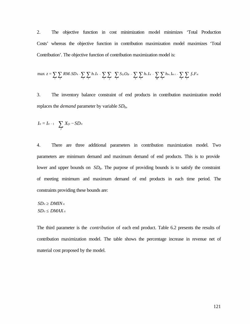
121
2. The objective function in cost minimization model minimizes ‘Total Production
Costs’ whereas the objective function in contribution maximization model maximizes ‘Total
Contribution’. The objective function of contribution maximization model is:
3. The inventory balance constraint of end products in contribution maximization model
replaces the demand parameter by variable SDit,
4. There are three additional parameters in contribution maximization model. Two
parameters are minimum demand and maximum demand of end products. This is to provide
lower and upper bounds on SDit. The purpose of providing bounds is to satisfy the constraint
of meeting minimum and maximum demand of end products in each time period. The
constraints providing these bounds are:
The third parameter is the contribution of each end product. Table 6.2 presents the results of
contribution maximization model. The table shows the percentage increase in revenue net of
material cost proposed by the model.
∑ −+= −
j
itijtitit SDXII 1
∑ ∑ ∑ ∑ ∑ ∑ ∑∑ ∑ ∑∑∑∑ −−−−−=i t i t s t m t s t
ststmstsijtij
j
iti
i t
iti FfhIhOSIhSDRMz .I.. max m...
itit DMINSD ≥
itit DMAXSD ≤

122
Table 6.2: Percentage Increase in ‘Revenue Net of Material Cost’ in Contribution
Maximization Model as Compared to the Actual Sales and Production Plan.
To meet the sales plan, table 6.3 below shows the improvement in production costs in the
contribution maximization model.
Table 6.3: Production Costs Difference In Percentage: (Actual Production Plan–
Production Plan Proposed by the Model)
6.69 Inventory Carrying Cost of By-Products and Raw Materials
6.38 Fresh Raw Material cost
24.79
Set-up Cost of Intermediates and End Products.
60.90
Inventory Carrying Cost of Intermediates and End Products.
42.54 Percentage Increase in Contribution
24.82 Percentage Increase in Revenue Net of
Material Cost
5.44 Percentage Increase in Materials Cost of Goods Sold
11.45 Percentage Increase in Sales

123
Savings due to jointly planning sales and production is Rupees 9.92 crores. This is
42.54 percent increase in contribution. Significantly higher benefits are realized in the case of
jointly planning sales and production over the production plan to meet the demand forecast.
It is interesting to see that with only 11.45 percent increase in model sales plan as
compared to actual sales (Table 6.2), reduction in production costs due to improved
production-planning (Table 6.3), results in 42.54 percent increase in contribution. There are
few issues to be analyzed for considerable increase in contribution proposed by the
contribution maximization model. The results indicate the operating philosophy of the
company. The notion followed by the company is to maximize the capacity utilization, rather
then to plan for the demand forecast. This leads to excess inventories of most of the products.
It is seen in results, that to meet the demand, reduction in inventory costs is a major
component of savings. This is one of the important insights for managers that producing to
capacity can lead to very high operational costs. The other reason for considerable
improvement in contribution is, obviously, more sales in the model results. There are upper
bounds on the demand, and it is assumed that the company would be able to realize the sales
suggested by the model. The contribution maximization model guides the marketing people
to sell a certain product mix, which will maximize the contribution of the firm. It is possible
that due to high demand variability, price competitiveness, and other market constraints,
sales plan suggested by the model may not be realized. There are other uncertainties in the
environment like machine breakdowns, rejections due to poor quality etc., which would
affect the actual contribution realization. In the next section, we describe the application of
scheduling model.
124
6.5 Application of Scheduling Model
In this section, we solve the scheduling problem. We apply the solution procedures
developed for solving scheduling problem in chapter 4. The production-planning model is an
input to the detailed scheduling model. As discussed in the product structure diagram,
products at level 0 are the finished goods. Finished goods are scheduled by applying the
solution procedure of flowshop E/T problems described in chapter 4. Finished goods derived
their due dates on the basis of customer orders and demand forecast. In this application,
finished goods have shipments several times in a month based on customer orders. Hence, we
apply the flowshop E/T scheduling problem in each week of the month. The common due
dates of finished goods is end of each week. The objective of the finished goods scheduling
is to minimize earliness and tardiness penalties. Intermediate products (Level 1 onwards)
derive their due dates from the schedule of higher-level products. The objective of
intermediate products scheduling is to minimize earliness penalties. As discussed in chapter
4, in solution procedure for intermediate products scheduling, tardiness is not allowed in the
intermediate products scheduling to maintain the feasibility of the schedule. This is because
while scheduling intermediate products at any level of product structure, the higher-level
products are already scheduled. Intermediate products have due date based on the start time
of higher-level products. Allowing tardiness would lend the schedule of higher-level product
infeasible. To solve intermediate products scheduling problem in this application, we apply
the solution procedure for solving the intermediate goods scheduling problem described in
chapter 4. For products produced on dedicated production plants, we apply the solution
procedure for scheduling dedicated plants discussed in chapter 4. A product has a standard
batch size. The number of batches to be produced is determined from the batch size of

125
products. Scheduling decisions determine the start time and completion time of each batch of
product on each machine. The detailed schedule of products and its earliness and tardiness
costs for each time period of the planning horizon are provided in appendix 3. In the next
section, we discuss sensitivity analysis on the results of the production planning ands
scheduling problem.
6.6 Sensitivity Analysis on Production Planning and Scheduling Results
In this section, we perform sensitivity analysis on the production planning and
scheduling results obtained in the previous section. Sensitivity analysis is done on demand of
finished goods, initial inventory of finished goods and intermediate products, capacity of
dedicated and flexible plants, and ratio of setup cost to inventory cost of intermediate
products and finished goods. Demand is chosen for sensitivity analysis as the environment
has demand variability, and sensitivity on demand will help in coordinating the marketing
decisions in a better way. Sensitivity on initial inventory will help in evaluating the cost of
purchasing the intermediate products as compared to in-house production to avoid production
delays. The instance solved in the previous section is considered as the base case. We are not
analyzing the sensitivity of parameters on scheduling costs, as they are very less as compared
to the production costs.
As shown in table 6.4, we observe the impact of change in parameters on inventory
costs and setup costs of intermediate products and finished goods, inventory costs of by-
products and reusable raw materials and cost of fresh raw material used. The detailed results
(production quantities of products and number of setups) of all the cases are provided in
appendix 3. We also observe the impact on capacity utilization of dedicated plants, and of

126
each machine in the flexible plants. Table 6.4 shows for each case, its production costs and
the change in costs from the base case. Demand of finished goods is varied from 80 percent
of the base case demand to 120 percent of the base case demand. The major factor that
reduces the cost at 80 percent of the base case demand is the cost of fresh raw material. The
inventory of intermediate products and finished goods are higher in case 2 as compared to
case 1, due to the high initial inventory of products. With increase in demand, the cost of
fresh raw material also goes up. Table 6.5 and table 6.6 indicate the capacity utilization in
percentage of dedicated plants and of machines in flexible plants respectively. In table 6.5,
for each case, the average capacity utilization of dedicated plant is shown. The average
capacity utilization is determined over the 5-month planning horizon. The average capacity
utilization of dedicated plants is reduced by around 30 percent at 80 percent base case
demand. In table 6.6, the average capacity utilization over a 5-month period is determined for
each machine in the flexible plant. The average capacity utilization of machines is reduced
by around 25 percent in the case of 80 percent base case demand. With increase in demand,
the capacity utilization of dedicated plants goes up by 20 percent and 15 percent in case of
flexible plants. The production plan is infeasible at 120 percent of the base case demand of
finished goods. At 120 percent of the base case demand, the capacity constraint of one of the
flexible machines gets violated.
The aggregate capacity of dedicated plants and machines of flexible plants is varied
from 80 percent to 120 percent of the base case capacity. It is seen that at 80 percent of the
base case capacity, the production plan is infeasible and is not able to meet the base case
demand. Reduction in capacity is resulting in high inventory costs. At 110 percent and 120
percent of the base case capacity, the production costs are decreasing. This is due to the

127
reduction in inventory costs and setup costs. Since capacity is more, the model is suggesting
to produce when required, resulting in less build up of inventory. It is seen in table 6.5 that
the capacity utilization of some of the dedicated plants is not very high. This is an important
observation to the management for capacity planning related issues. One of the reasons for
low capacity utilization could be the seasonality in the demand of products produced in these
plants. In the five months instance solved, the products produced in low capacity utilization
plants may have less demand. Another insight from this result is that some reallocation of the
capacity is required to improve the overall capacity utilization of the production plants. Low
capacity utilization is also an indication to the marketing department to enhance the sales of
the products produced in these plants. Sensitivity on capacity is also useful for long-term
strategic decisions for the company. Marginal value of the capacity is an useful indicator to
the management for determining the appropriate capacity of the resources.
Impact of initial inventory is significant on the production plan costs and capacity.
Initial inventory of intermediate products and finished goods is varied from 80 percent to 120
percent of the base case. With high initial inventory, reduction in total costs is seen in table
6.4. At 120 percent of the base case initial inventory, although the inventory costs go up, the
cost of fresh raw material reduces (due to less production of products) considerably. This
reduces the overall cost of case 14. The inventory costs are rising with increase in inventory
due more to inventory being carried over in the planning horizon. The capacity utilization
decreases with increase in initial inventory. With less initial inventory, the production costs
increase due to more consumption of fresh raw materials. This is happening because more
production is required with less initial inventory. Capacity utilization is also increasing with
less initial inventory.

128
Sensitivity is also done on ratio of setup costs to inventory costs. It is seen that with
more setup to inventory costs ratio (cases 15; 16), the number of setups decrease (as seen in
reduced setup costs). The inventory costs in these cases increase resulting in overall increase
of costs. This is because in the production plan, more inventory is carried due to high setup
costs. The production plan changes in both the cases. In cases 17 and 18, there is no change
in the production plan. However, the production costs reduce due to significantly less use of
fresh raw material. The inventory of by-products and reusable raw material is also less in
cases 17 and 18.
6.7 Implementation Issues
The benefits of production planning model were shown to the company from the
results of five-month data. The benefits provided the motivation to the management for
implementing the models. The extent of savings due to production planning model is
presently difficult to estimate over a longer duration. The company is in the process of using
the production planning and scheduling models for their complete operations. Presently, the
implementation of scheduling model is not fully functional.
On-site training was provided to the personnel involved in planning and shop floor
scheduling. The Decision Support System (DSS) developed was documented to include;
production-planning and scheduling problem, key decisions in the problem, structure of
production planning and scheduling models, interpretation of results, and sensitivity analysis
on results. The planning model developed in GAMS was provided interface with Microsoft
Excel to import the parameters of the model. This was also done to facilitate the change in
parameters with ease.

129
One major observation from implementation of the models is that managers do not
easily internalize the benefits of optimization tools. We faced difficulties in convincing the
plant managers that producing just to increase capacity utilization often results in high
operational costs. The results of the models helped managers to understand the importance of
this issue. Another important issue we experienced in implementation of these models is that
right training and competence is imperative to exploit maximum benefits of optimization
tools. It is very important for the users to know the capabilities of such decisions support
systems.
6.8 Summary
In this chapter, we have solved a real life large-scale complex production planning
and scheduling problem of a pharmaceutical company. We have applied the mathematical
models developed in chapter 3 to address the production planning and scheduling decisions
of the problem. The solution procedure developed for solving production planning and
scheduling problem were applied to solve the problem in this application. In section 6.3, the
application of production planning model is described. The results of the production-planning
model over the finite planning horizon have shown considerable savings in the production
costs over the actual production plan of the company. A variant of the production-planning
model is developed in section 6.4. This model is for jointly planning sales and production. It
is shown that significant increase in the savings is realized in the sales and production plan
over the plan to meet just the demand forecast. Application of scheduling model is discussed
in section 6.5. The solution procedure and results of the scheduling model are described in
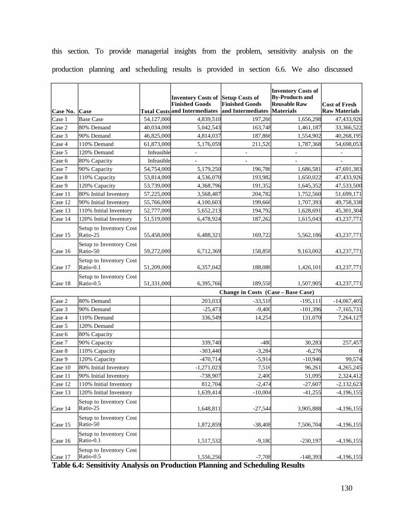
130
this section. To provide managerial insights from the problem, sensitivity analysis on the
production planning and scheduling results is provided in section 6.6. We also discussed
Case No. Case Total Costs
Inventory Costs of Finished Goods and Intermediates
Setup Costs of Finished Goods and Intermediates
Inventory Costs of By-Products and Reusable Raw Materials
Cost of Fresh Raw Materials
Case 1 Base Case 54,127,000 4,839,510 197,266 1,656,298 47,433,926Case 2 80% Demand 40,034,000 5,042,543 163,748 1,461,187 33,366,522Case 3 90% Demand 46,825,000 4,814,037 187,866 1,554,902 40,268,195Case 4 110% Demand 61,873,000 5,176,059 211,520 1,787,368 54,698,053Case 5 120% Demand Infeasible - - - - Case 6 80% Capacity Infeasible - - - - Case 7 90% Capacity 54,754,000 5,179,250 196,786 1,686,581 47,691,383Case 8 110% Capacity 53,814,000 4,536,070 193,982 1,650,022 47,433,926Case 9 120% Capacity 53,739,000 4,368,796 191,352 1,645,352 47,533,500Case 11 80% Initial Inventory 57,225,000 3,568,487 204,782 1,752,560 51,699,171Case 12 90% Initial Inventory 55,766,000 4,100,603 199,666 1,707,393 49,758,338Case 13 110% Initial Inventory 52,777,000 5,652,213 194,792 1,628,691 45,301,304Case 14 120% Initial Inventory 51,519,000 6,478,924 187,262 1,615,043 43,237,771
Case 15 Setup to Inventory Cost Ratio-25 55,458,000 6,488,321 169,722 5,562,186 43,237,771
Case 16 Setup to Inventory Cost Ratio-50 59,272,000 6,712,369 158,858 9,163,002 43,237,771
Case 17 Setup to Inventory Cost Ratio-0.1 51,209,000 6,357,042 188,086 1,426,101 43,237,771
Case 18 Setup to Inventory Cost Ratio-0.5 51,331,000 6,395,766 189,558 1,507,905 43,237,771
Change in Costs (Case – Base Case) Case 2 80% Demand 203,033 -33,518 -195,111 -14,067,405Case 3 90% Demand -25,473 -9,400 -101,396 -7,165,731Case 4 110% Demand 336,549 14,254 131,070 7,264,127Case 5 120% Demand Case 6 80% Capacity Case 7 90% Capacity 339,740 -480 30,283 257,457Case 8 110% Capacity -303,440 -3,284 -6,276 0Case 9 120% Capacity -470,714 -5,914 -10,946 99,574Case 10 80% Initial Inventory -1,271,023 7,516 96,261 4,265,245Case 11 90% Initial Inventory -738,907 2,400 51,095 2,324,412Case 12 110% Initial Inventory 812,704 -2,474 -27,607 -2,132,623Case 13 120% Initial Inventory 1,639,414 -10,004 -41,255 -4,196,155
Case 14 Setup to Inventory Cost Ratio-25 1,648,811 -27,544 3,905,888 -4,196,155
Case 15 Setup to Inventory Cost Ratio-50 1,872,859 -38,408 7,506,704 -4,196,155
Case 16 Setup to Inventory Cost Ratio-0.1 1,517,532 -9,180 -230,197 -4,196,155
Case 17 Setup to Inventory Cost Ratio-0.5 1,556,256 -7,708 -148,393 -4,196,155
Table 6.4: Sensitivity Analysis on Production Planning and Scheduling Results
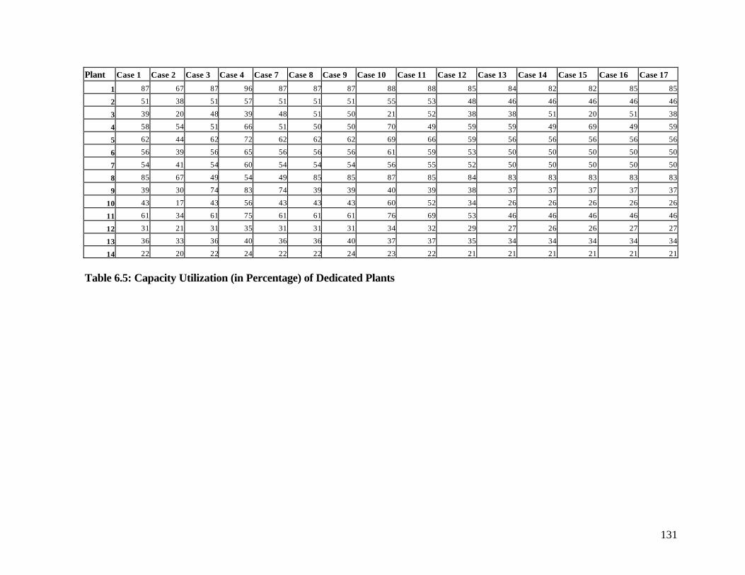
131
Plant Case 1 Case 2 Case 3 Case 4 Case 7 Case 8 Case 9 Case 10 Case 11 Case 12 Case 13 Case 14 Case 15 Case 16 Case 17
1 87 67 87 96 87 87 87 88 88 85 84 82 82 85 85
2 51 38 51 57 51 51 51 55 53 48 46 46 46 46 46
3 39 20 48 39 48 51 50 21 52 38 38 51 20 51 38
4 58 54 51 66 51 50 50 70 49 59 59 49 69 49 59
5 62 44 62 72 62 62 62 69 66 59 56 56 56 56 56
6 56 39 56 65 56 56 56 61 59 53 50 50 50 50 50
7 54 41 54 60 54 54 54 56 55 52 50 50 50 50 50
8 85 67 49 54 49 85 85 87 85 84 83 83 83 83 83
9 39 30 74 83 74 39 39 40 39 38 37 37 37 37 37
10 43 17 43 56 43 43 43 60 52 34 26 26 26 26 26
11 61 34 61 75 61 61 61 76 69 53 46 46 46 46 46
12 31 21 31 35 31 31 31 34 32 29 27 26 26 27 27
13 36 33 36 40 36 36 40 37 37 35 34 34 34 34 34
14 22 20 22 24 22 22 24 23 22 21 21 21 21 21 21
Table 6.5: Capacity Utilization (in Percentage) of Dedicated Plants

132
EQ1 31 21 26 35 31 31 30 34 33 29 27 25 24 27 27EQ2 23 14 19 27 23 23 23 28 26 21 18 18 17 19 19
EQ3 52 31 41 38 55 49 39 57 53 47 28 24 53 32 30
EQ4 63 40 47 59 60 52 53 57 53 51 49 49 49 59 49EQ5 55 37 46 66 55 55 55 65 60 50 46 47 46 47 46
EQ6 32 33 39 73 32 45 56 48 46 42 55 58 28 43 54
EQ7 53 37 45 63 53 53 53 61 57 49 46 46 46 47 46EQ8 68 50 60 78 68 68 68 73 70 66 64 63 63 64 64
EQ9 0 0 0 0 0 0 0 0 0 0 0 0 0 0 0
EQ10 51 37 44 58 51 51 50 56 54 48 44 44 43 46 45EQ11 0 0 0 0 0 0 0 0 0 0 0 0 0 0 0
EQ12 57 40 48 68 57 57 58 65 61 54 51 50 50 51 51
EQ13 44 33 39 50 44 44 44 46 45 42 40 41 40 41 40EQ14 0 0 0 0 0 0 0 0 0 0 0 0 0 0 0
EQ15 18 10 14 22 18 18 18 24 21 15 12 12 11 13 13
EQ16 56 46 51 61 56 56 56 56 56 56 56 56 55 56 56EQ17 55 45 50 60 55 55 55 55 55 55 55 55 54 55 55
EQ18 50 41 45 54 49 49 49 50 50 50 50 49 49 51 50
EQ19 50 40 45 54 50 50 50 50 50 50 50 50 49 49 50EQ20 3 2 2 3 3 3 3 3 3 3 3 3 2 2 3
EQ21 2 1 2 2 2 2 2 2 2 2 2 2 2 2 2
EQ22 38 31 35 41 38 38 38 38 38 39 39 39 37 38 39EQ23 50 40 45 54 50 50 50 50 50 50 50 50 49 49 50
EQ24 58 47 52 63 57 57 57 58 58 58 58 57 56 58 58
EQ25 56 45 51 62 56 56 56 56 56 57 57 57 56 56 57EQ26 49 40 45 54 49 49 49 50 50 50 50 50 49 49 50
EQ27 50 40 45 55 50 50 50 50 50 50 50 50 50 50 50
EQ28 58 47 52 63 57 57 57 58 58 58 58 57 56 58 58EQ29 68 54 61 74 67 67 67 68 68 67 67 67 66 68 67
EQ30 53 41 47 58 52 52 52 53 53 53 53 52 52 53 53
EQ31 55 45 50 60 55 55 55 55 55 55 55 55 54 55 55
Table 6.6: Capacity Utilization (in Percentage) of Machines in Flexible Plants

133
some issues regarding implementation of the models. In the next chapter, we provide
conclusions of this research. We also discuss issues relevant to future research from this
thesis.

134
7 Summary, Contribution and Future Research
7.1 Summary
In this research, we investigate the potential of production planning and scheduling in
reducing the operational costs of manufacturing firms with complex production environment.
We discussed that manufacturing firms are facing complexities in form of increasing product
variety, shrinking product volumes, demand variability, and increase in customer response
times. As a result, firms are paying high attention to the operating costs. In this context, we
discussed that production planning and scheduling can contribute significantly in reducing
the operating costs of firms.
Motivated by the complex production environment of chemical plants, we consider
the production planning and scheduling problem existing in process industries and discrete
parts manufacturing industries. We consider multi-stage, multi-product, multi-machine and
batch processing production environment. We model the production planning and scheduling
decisions in two steps. In the first step, we develop production-planning model, which is
mixed integer linear programme (MIP). The decisions of the production model are to
determine production quantity of products, inventory levels of products, and to determine the
aggregate capacity of resources required to meet the production plan. The objective of the
production-planning model is to minimize the production costs over the planning horizon. In
the second step, we model scheduling decisions. There are two scheduling MIP models,
finished goods scheduling model and intermediate products scheduling model. This is
because in the production environment, finished goods follow flowshop setting and
intermediate products follow jobshop setting with re-entrant flows. The decisions of

135
scheduling model are to determine start time and completion times of all products on each
machine. The objective of scheduling model is to minimize the earliness and tardiness
penalties. The production-planning decisions impose constraints, within which the detailed
scheduling decisions are made.
We solve the production-planning problem using the branch and bound algorithm.
For finished goods scheduling, we consider the permutation flowshop problem with common
due date. The problem is NP-complete. Based on the common due dates, the finished goods
scheduling problem can be decomposed in three sub-problems; sub-problem 1 with
unrestricted due date, sub-problem 2 with intermediate due date, and sub-problem 3 with
restricted due date. Using some of the known optimal results of single machine earliness and
tardiness problem, we develop procedures to determine unrestricted, intermediate and
restricted due dates in multi-machine environment. The objective of all the three sub-
problems is to minimize the absolute deviation of job completion times from a common due
date. We derive analytical results for solving sub-problem 1.
We develop heuristic algorithms to solve sub-problem 2. The heuristic derives a
permutation flowshop sequence at the bottleneck machine. The pre-bottleneck bottleneck
processing times are treated as release dates of jobs at the bottleneck. The post-bottleneck
processing times are considered to derive due dates of jobs at the bottleneck machine. By
solving single machine problem with release dates and due dates iteratively at the bottleneck
machine, we derive a permutation flowshop sequence. Then, we apply tabu search methods
to improve the solution. There are no previous results available in the literature of sub-
problems 1 and 2, i.e., flowshop scheduling problems minimizing absolute deviation of jobs
from a common due date. For small problem instances, we determine optimal solution of

136
sub-problem 2, using branch and bound algorithm. We show that the lower bound of sub-
problem 2 is very weak, as the average percentage deviation of optimal solution from lower
bound is very high (326 percent for n = 5, m = 5, 50 instances; 284 percent for n = 10; m = 5,
50 instances). For small problems, we compare the performance of heuristic solution with the
optimal solution. The average percentage deviation of heuristic solution from optimal
solution is 0.894 percent for n = 5, m = 5, 50 instances and 1.126 percent for n = 10, m = 5,
50 instances respectively. For large problems, we compare the heuristic performance with the
analytical solution of sub-problem 1 obtained in polynomial time. The average percentage
deviation of the largest problem instance solved (n = 100, m = 20, 50 instances) is 1.129
percent.
We develop heuristic algorithm for sub-problem 3. Sub-problem 3 is the flowshop
problem of minimizing earliness and tardiness penalties, with restricted common due date.
Sub-problem 3 has a special structure, that by definition of restricted due date, no job is
early. The objective of sub-problem 3 reduces to minimize tardiness. If all jobs are tardy and
simultaneously available with non-positive release dates, minimizing tardiness is same as
minimizing flow time or minimizing completion time. There are results available in the
literature on minimizing tardiness, minimizing flow time and minimizing completion time in
permutation flowshops. We compare our heuristic results with some of the best-known
results of these problems and found our heuristic to perform better. We applied our heuristic
results and the existing results on some benchmark problems in the literature on flowshop
scheduling. The average percentage deviation of our heuristic solution from the lower bound
of sub-problem 3 is found to be less than the solution of existing heuristics.

137
Then, we solve the intermediate products scheduling problem. The production
process of intermediate products is a general job shop setting wit re-entrant flows.
Intermediate products have derived demand. To maintain feasibility of scheduling decisions,
we do not allow tardiness in the intermediate products schedule. This is because intermediate
products derive their due dates from the existing schedule of the higher-level products, where
the intermediate products are consumed. We develop heuristics to solve the intermediate
products scheduling problem. The heuristic is developed with an objective of minimizing
earliness costs, i.e., the completion time of a job is as close as possible to the due date. As
discussed above, the completion time cannot exceed the due date to maintain feasibility. The
heuristic determines the schedule of intermediate products at all levels in the product
structure.
We report the results of production planning and scheduling problem. The data is
provided by a large pharmaceutical company in India. We obtain optimal production plan
over a finite planning horizon, consisting of production quantity and inventory levels of
intermediate products and finished goods, inventory levels of by-products and reusable raw
materials and amount of fresh raw materials used in the production process. We determine
aggregate capacity of resources required to meet the production plan. We obtain scheduling
decisions; start time and completion times of each intermediate product and each end product
on each machine. We also determine the earliness and tardiness costs in the schedule.
We apply the production planning and scheduling models in a pharmaceutical
company in India. This application has multi-stage, multi-product, multi-machine, batch
production environment. We implement the solution procedure developed for solving
production planning and scheduling problem on 5-month data (January, 2002 to May, 2002).

138
In this instance, there are 10 finished goods, 30 intermediate products and 15 production
lines. We compare the results of the production-planning model with the actual production
plan followed by the company during the 5-month period. The total savings due to improved
production planning using the production planning model over the actual production plan
followed by company are Rupees.2.60 crores. The savings in the plan proposed by the
production-planning model while maintaining the supply of end products at par with actual
production (i.e., cumulative demand in this case is same as that in actual production case) are
Rupees 1.90 crores. We also develop a variant of the production-planning model with
additional market constraints. The model is used for jointly planning sales and production,
and it maximizes contribution. Based on the lower and upper bounds on demand, this model
suggests the best sales mix that will maximize contribution. Savings in contribution using the
contribution maximization model sales and production plan are Rupees 9.92 crores. The
results show that savings can be significantly increased by using the model for joint planning
of sales and production over the production plan to meet the demand forecast. We report
results on scheduling the production plan proposed by the production-planning model. We
determine start time and completion time of each product in the production plan on each
machine. Earliness and tardiness costs of the products are determined in the schedule. We
also perform sensitivity analysis on the production planning and scheduling results in this
application. In sensitivity analysis, we study the impact of aggregate capacity, demand, initial
inventory and ratio of setup to inventory costs. The production planning and scheduling
models are presently being used by the company.
In this research, we have shown the tangible benefits of production planning and
scheduling in complex manufacturing environment. We have solved large and difficult
139
production planning and scheduling problems faced by manufacturing firms today. We have
derived some new analytical results and proposed new heuristic algorithms for a class of
production planning and scheduling problems. We expect that models developed in this
research would form basis for production planning and scheduling decisions in complex
production environments. Sensitivity analysis on the results would help the managers to
evaluate alternate production plans and schedules and manage the complexities in the
environment in a better way. In the next section, we discuss the contribution of this research.
7.2 Contribution
• In this research, we address the decisions of complex production planning and
scheduling problems existing in discrete parts manufacturing industries and process
industries. We consider a multi-stage, multi-product, multi-machine batch-processing
environment.
• We consider some new complexities in the production environment that have not
been addressed in the literature on production planning and scheduling. In our
problem, the production environment produces finished goods and intermediate
products. By-products are generated from finished goods and intermediate products,
and are recycled to recover reusable raw materials. Traditional models on multi-stage
production planning and scheduling, are primarily based on assembly and fabrication
types of product structures. We consider the complexity of recycling process in the
product structures. There are flexible machines in the production environment. The
machines are used for processing both finished goods and intermediate products,
which complicates the scheduling decisions considerably. The production

140
environment faces demand forecast over the finite planning horizon. Finished goods
in the environment follow flowshop type of production process, and intermediate
products follow general jobshop type of production process with re-entrant flows.
• We model the production planning and scheduling decisions through sequence of
hierarchical models. First, we develop a mixed integer program (MIP) for production
planning decisions. The objective of the production-planning model is to minimize
inventory costs and setup costs of intermediate products and finished goods,
inventory costs of by-products and reusable raw materials, and cost of fresh raw
material. In the next step, we develop an MIP for finished goods scheduling
decisions. Then, we develop an MIP for intermediate products scheduling problem
decisions. The objective of the scheduling problem is to minimize the absolute
deviation of job completion times from a common due date.
• The production-planning problem is solved using the branch and bound algorithm.
We report some new results for solving the scheduling problem. Finished goods
scheduling (flowshop) problem of minimizing absolute deviation of job completion
times from a common due date is not addressed in the literature. We develop
analytical results for solving flowshop scheduling problem in certain ranges of
common due dates. We also develop new heuristic algorithms for flowshop problem,
where obtaining analytical solution is difficult. For flowshop earliness and tardiness
problems with special structure (minimizing tardiness, flowtime, completion time),
we develop new heuristic algorithm for the problems. We compare the heuristic
algorithms for this class of problems with some of the best existing results. The
computational performance of our heuristics is found to be better that those of

141
existing heuristics. We develop heuristic algorithms for solving the intermediate
products scheduling problem.
• We report implementation of the production planning and scheduling models in a real
life case of a pharmaceuticals company in India. The results of the models indicate
substantial savings over the actual company performance. Sensitivity analysis on the
results is provided evaluate various production plans and schedules. In the next
section, we identify certain issues which we have not considered in this research, and
which deserve attention in future research from this work.
7.3 Future Research
In this research, we have decomposed the overall production planning and scheduling
problem and developed sequential models to address the decisions in the problem. One
possible natural extension of this research would be to exploit further the benefits of
decision-making in hierarchical production planning. We have not considered the
aggregation of products, as mentioned in Bitran and Tirupati (1993). Products may be
aggregated into families, and families into types. A type is a collection of products with
similar demand patterns and production rates. A family is a set of products within a type such
that products in the family share a common setup. Advantages of aggregation of products
will be less dimensionality of mathematical programs, less detailed demand forecast will be
required (for product types only). The next process will be to develop disaggregation models
to determine the production plans for product families. Further disaggregation of the family
production lots to determine the quantities of product will be required.

142
Another useful extension of this work could be to analyze uncertainties in production
situations. Some of the uncertainties in the form of machine failures and demand forecast
errors often exist in real life situations. Production planning and scheduling with stochastic
demand would be a good generalization of this research. Situations like variability in
processing times of jobs and variability in process yields are very common, especially in
process industries. We have focused primarily on deterministic scheduling in this research.
The information about the problem instances is known with certainty in deterministic
scheduling. Modeling scheduling decisions with stochastic parameters would help in
capturing some common uncertainties in scheduling.
We have considered permutation flowshop environment for finished goods
scheduling, and common due dates of finished goods. Analysis of general flowshop setting
and considering distinct due dates of products will be very useful extension of this work.
For flowshop problems where it was difficult to obtain analytical solution, we have
developed heuristic algorithms. It will be a useful contribution to determine the theoretical
performance guarantee of the heuristics.
Finally, one very important extension of this research would be to study the issues
involved in solving the production planning and scheduling problem, as an integrated
problem. A monolithic model for addressing production planning and scheduling decisions is
difficult to solve. The computational effort required to solve is also enormous. Another issue
in an integrated problem solving approach will be to ensure consistency between the
production planning decisions, and scheduling decisions. A useful comparison will be the
quality of the solution in hierarchical problems as compared to the integrated production

143
planning and scheduling problem. To prove the decomposition approach of solving the
production planning and scheduling problem, as a valid lower bound on the overall problem
will be another important and interesting issue of research.

144
References
Abdul-Razaq, T. S. and C. N. Potts, “Dynamic Programming in State-Space Relaxation for
Single Machine Scheduling”, Journal of Operations Research Society, 39. 1988, 141-152.
Akthar, P. “ACCPAC Streamlines Synpack’s Manufacturing Processes”, Express Computer,
India Express Newspapers Ltd., 2004.
Afentakis, P., B. Gavish and U. Karmarkar, “Computationally Efficient Optimal Solutions to
the Lot-Sizing Problem in Multi-Stage Systems”, Management Science, 30(2). 1984, 222-
239.
Afentakis, P. and B. Gavish, “Optimal Lot-Sizing for Complex Product Structures”,
Operations Research, 34(2). 1986, 237-249.
Ahmadi, R. H. and U. Bagchi, “Improved Lower Bounds for Minimizing the Sum of
Completion Times of n Jobs over m Machines in a Flowshop”, European Journal of
Operational Research, 44. 1990, 331-336.
Bagchi, U., R. Sullivan and Y. Chang, “Minimizing Mean Absolute Deviation of Completion
Times about a Common Due Date”, Naval Research Logistics Quarterly, 33. 1986, 227-240.
Bagchi, U., Y. Chang and R. Sullivan, “Minimizing Absolute and Squared Deviations of
Completion Times with Different Earliness and Penalties and a Common Due Date”, Naval
Research Logistics Quarterly, 34. 1987, 739-751.
Bagchi, U., R. Sullivan and Y. Chang, “Minimizing Mean Squared Deviation of Completion
Times About a Common Due Date”, Management Science, 33. 1987, 894-906.
Bahl, H. C., L. P. Ritzman and J. D. N. Gupta, “Determination of Lot-Sizes and Resource
Requirements”, Operations Research, 35. 1987, 329-345.
Baker, K. R. and G. D. Scudder, “Sequencing with Earliness and Tardiness Penalties: A
Review”, Operations Research, 38(1). 1990, 22-36.
Baker, T. E. and L. S. Lasdon, “Successive Linear Programming at Exxon”, Management
Science, 31. 1985, 264-272.

145
Bector, C., Y. Gupta and M. Gupta, “Determination of an Optimal Common Due Date and
Optimal Sequence in a Single Machine Job Shop”, International Journal of Production
Research, 26. 1988, 613-628.
Billington, P. J., J. O. McClain and L. J. Thomas, “Mathematical Approaches to Capacity
Constrained MRP Systems: Review, Formulation and Problem Reduction”, Management
Science, 29. 1983,1126-1141.
Bitran, G. R. and A. C. Hax, “On the Design of Hierarchical Production Planning Systems”,
Decision Sciences, 8. 1977, 28-55.
Bitran, G. R. and D. Tirupati, “Hierarchical Production Planning”, Chapter 10 in S. C.
Graves et al. (eds.), Handbooks in Operations Research and Management Science. Vol. 4,
Elsevier Science, 1993, 523-566.
Bitran, G. R. and D. Tirupati, “Planning and Scheduling For Epitaxial Wafer Production
Facilities”, Operations Research, 36(1). 1998a, 34-49.
Bitran, G. R. and D. Tirupati, “Development and Implementation of a Scheduling System:
An Application in a Wafer Fabrication Facility”, Operations Research, 36(3). 1998b, 377-
395.
Bitran, G. R., E. A Haas and A. C. Hax, “Hierarchical Production Planning: A Single Stage
System”, Operations Research, 29. 1981, 717-743.
Bitran, G. R., E. A Haas and A. C. Hax, “Hierarchical Production Planning: A Two-Stage
System”, Operations Research, 30. 1982, 232-251.
Blackburn, J. and R. Millen, “Improved Heuristics for Multi-Stage Requirements Planning”,
Management Science, 28(1). 1982, 44-46.
Blomer, F. and H. O. Gunther, “Scheduling of a Multi-Product Batch Process in a Chemical
Industry”, Computers in Industry, 36. 1998, 245-259.
Bowers, M. R. and J. P. Jarvis, “A Hierarchical Production Planning and Scheduling Model”,
Decision Sciences, 23(1). 1992, 144-158.

146
Bradley, S.P, A. C. Hax and T. L. Magnanti, “Integration of Strategic and Tactical Planning
in the Aluminum Industry”, Chapter 6 in Applied Mathematical Programming, Edison
Wesley, Reading, MA, 1977.
Chao, H., S. Chapel, C. Clark, P. Morris, M. Sandling and R. Grimes, “EPRI Reduces Fuel
Inventory Costs in the Electric Utility Industry”, Interfaces, 19(1). 1989, 48-67.
Cheng, T, “Optimal Due Date Determination and Sequencing of n Jobs on a Single
Machine”, Journal of Operations Research Society, 35. 1984, 433-437.
Cheng, T, “An Algorithm for the Due Date Determination and Sequencing Problem”,
Computers and Operations Research, 14. 1987, 537-542.
Cheng, T.C.E. and H. G. Kahlbacher, “A Proof of the Longest-First Job Policy in One
Machine Scheduling”, Naval Research Logistics Quarterly, 38. 1991, 715-720.
Conway, R.W., W.L. Maxwell and L.W. Miller, Theory of Scheduling, Addison-Wesley,
MA, 1967.
Chu, C., “A Branch and Bound Algorithm to Minimize Total Tardiness with Different
Release Dates”, Naval Research Logistics Quarterly, 39. 1992, 265-283.
Chu, C. and M. C. Portmann, “Some New Efficient Methods to Solve n/1/ri/? Ti Scheduling
Problem”, European Journal of Operation Research, 58. 1992, 404- 413.
Crama, Y., Y. Pochet and Y. Wera, “A Discussion of Production Planning Approaches in the
Process Industries”, Production and Inventory Management, 31(3). 2001, 462-480.
Crowston, W. P., M. H. Wagner and J. F. Williams, “Economic Lot-Size Determination in
Multi-Stage Systems”, Management Science, 19. 1973, 517-527.
Crowston, W. P. and M. H. Wagner, “Dynamic Lot-Size Models for Multi-Stage Assembly
Systems”, Management Science, 20. 1973,13-21.
Dudek, R. A., S. S. Panwalkar and M. L. Smith, “The Lessons of Flowshop Scheduling”,
Operations Research, 40. 1992, 7-13.
De, P., J. B. Ghosh and C. E. Wells, “A Note on the Minimization of Mean Squared
Deviation of Completion Time about Common Due Date”, Management Science, 35. 1990,
1143-1147.

147
Dzielinski, B. P. and R. E. Gomory, “Optimal Programming of Lot-Sizes, Inventory and
Labor Allocations”, Management Science, 11. 1965, 874-890.
Eilon, S, “Multi-Product Scheduling in a Chemical Plant”, Management Science, 26. 1969,
669-678.
Eilon, S. and I. G. Chowdhury, “Minimizing Waiting Time Variance in the Single Machine
Problem”, Management Science, 23. 1977, 567-575.
Emmons, H, “Scheduling to a Common Due Date on Parallel Common Processors”, Naval
Research Logistics Quarterly, 34. 1987, 803-810.
Eppen, G. D. and R. K. Martin, “Solving Multi-Product Capacitated Lot-Sizing Problems
Using Variable Reduction”, Operations Research, 35. 1987, 832-848.
Feigin, G., A. Chae, D. Connors and I. Crawford, “Shape Up, Ship Out”, OR/MS Today,
23(2). 1996, 53-56.
Franca, P.M., V.A. Armentano, R.E. Berretta and A.R. Clark, “A Heuristic Method for Lot-
Sizing in Multi-Stage Systems”, Computers and Operations Research, 24. 1997, 861-874.
Francoo, J. C. and W. Rutten, “A Typology of Production Control Situations in Process
Industries”, International Journal of Operations and Production Management, 14. 1994, 47-
57.
Fry, T., R. Armstrong and J. Blackstone, “Minimizing Weighted Absolute Deviation in
Single Machine Scheduling Problem”, IEEE Transactions, 19. 1987, 445-450.
Gabbay, H., “Multi-Stage Production Planning”, Management Science, 25. 1979, 323-329.
Garey, M. R., D. S. Johnson and R. Sethi, “The Complexity of Flowshop and Jobshop
Scheduling”, Mathematics of Operation Research, 1. 1976, 117-129.
Garey, M. R., R. E. Tarjan and G. T. Wilfong, “One-Processor Scheduling with Symmetric
Earliness and Tardiness Penalties”, Mathematics of Operations Research, 13. 1988, 330-348.
Gowrishankar, K., C. Rajendran and G. Srinivasan, “Flowshop Scheduling Algorithms for
Minimizing the Completion Time Variance and the Sum of Squares of Completion Time
deviations from a Common Due Date”, European Journal of Operational Research, 132.
2001, 643-665.

148
Graves, S.C., A.H.G. Rinnooy Kan and P. H. Zipkin, “Logistics of Production and
Inventory”, Handbooks in Operations Research and Management Science, Vol 4, Elsevier
Science, 1993.
Gupta, S., and T. Sen, “Minimizing a Quadratic Function of Job Lateness on a Single
Machine”, Engineering Costs and Production Economics, 7. 1983,181-194.
Gupta, M. C., Y. P. Gupta and C. R. Bector, “Minimizing the Flow-time Variance in Single-
Machine Systems, Journal of Operational Research Society, 41. 1990, 767-779.
Gupta, S. D, “A Well-Tiled Path to Productivity”, Express Computer, India Express
Newspapers Ltd., 2003.
Hall, N, “Single and Multi-Processor Models for Minimizing Completion Time Variance”,
Naval Research Logistics Quarterly, 33. 1986, 49-54.
Hall, N., and M. E. Posner, “Earliness-Tardiness Scheduling Problems I: Weighted Deviation
of Completion Times about a Common Due Date”, Operations Research, 39. 1991, 836-846.
Hall, N., W. Kubiak and S. Sethi, “Earliness-Tardiness Scheduling Problems II: Deviation of
Completion Times about a Restrictive Common Due Date”, Operations Research, 39. 1991,
847-856.
Hax, A. C., and H.C Meal, “Hierarchical Integration of Production Planning and
Scheduling”, in M. A. Geisler (eds.). Studies in Management Studies. Vol.1: Logistics,
Elsevier, New York. 1975.
Johnson, S. M., “Optimal Two and Three Stage Production Schedules with Setup Times
Included”, Naval Research Logistics Quarterly, 1. 1954, 69-81.
Kahlbacher, H. G., “SWEAT – A Program for a Scheduling Problem with Earliness and
Tardiness Penalties”, European Journal of Operational Research, 43. 1989, 111-112.
Kanet, J., “Minimizing the Average Deviation of Job Completion Times About a Common
Due Date”, Naval Research Logistics Quarterly, 28(4). 1981a, 643-651.
Kanet, J, “Minimizing Variation of Flow Time in Single Machine Systems”, Management
Science, 27. 1981b, 1453-1459.

149
Kanet, J. and V. Sridharan, “Scheduling with Inserted Idle Time: Problem Taxonomy and
Literature Review”, Operations Research, 48. 2000, 99-110.
Karimi, B., S. Ghomi and J. Wilson, “The Capacitated Lot Sizing Problem: A Review of
Models and Algorithms, Omega, 31. 2003, 365-378.
Katayama, H., “On a Two-Stage Hierarchical Production Planning System for Process
Industries”, International Journal of Production Economics, 44(1). 1996, 63-72.
Kim, Y. D., “A New Branch and Bound Algorithm for Minimizing Mean Tardiness in Two-
Machine Flowshops”, Computers and Operations Research, 20. 1993, 391-401.
Kim, Y. D., “Heuristics for Flowshop Scheduling Problems: Minimizing Mean Tardiness”,
Journal of Operational Research Society, 44. 1993, 19-28.
Kim, Y. D., “Minimizing Total Tardiness in Permutation Flowshops”, European Journal of
Operational Research, 85. 1995, 541-555.
Kleutghen, P.P., and J. C. McGee, “Development and Implementation of an Integrated
Inventory Management Program at Pfizer Pharmaceuticals”, Interfaces, 15(1). 1985, 69-87.
Koulamas, C., “The Total Tardiness Problem: Review and Extensions”, Operations
Research, 42(6). 1994,1025-1041.
Koulamas, C. and Kyparisis, G., “Single machine Scheduling with Release Time, Deadlines
and Tardiness Objectives”, European Journal of Operational Research, 133. 2001, 447-453.
Kubiak, W., “Completion Time Variance Minimization on a Single Machine is Difficult”,
Operations Research Letters, 14. 1993, 49-59.
Kubiak, W, “New Results on the Completion Time Variance Minimization”, Discrete
Applied Mathematics, 58. 1995, 157-168.
Lambrecht, M., and M. VanderEecken, “A Facilities in Series Capacity Constrained
Dynamic Lot-Size Model”, European Journal of Operational Research, 2(2). 1978, 963-971.
Lasdon, L. S and R. C. Terjung, “An Efficient Algorithm for Multi-Product Scheduling”,
Operations Research, 19(4). 1971, 946-969.

150
Lakshminarayan, S., R. Lakshmanan, L. Papineau and R. Rochette, “Optimal Single Machine
Earliness and Tardiness Penalties”, Operations Research, 26. 1978, 1079-1082.
Leachman, R., R. Benson, C. Liu and D. Raar, “IMPReSS: An Automated Production-
Planning and Delivery-Quotation System at Harris Corporation-Semiconductor Industry”,
Interfaces, 26(1). 1996, 6-37.
Leong, G. K., M. D. Oliff and R. E. Markland, “Improved Hierarchical Production Planning
Model”, Journal of Operations Management, 8(2). 1989, 90-114.
Li, G., “Single Machine Earliness and Tardiness Scheduling”, European Journal of
Operational Research, 96. 1997, 546-558.
Liberatore, M. J. and T. Miller, “A Hierarchical Production Planning System”, Interfaces,
15(4). 1985, 1-11.
Lin, C. and C. L. Moodies., “Hierarchical Production Planning for a Modern Steel
Manufacturing System”, International Journal of Production Research, 27(4). 1989, 613-628.
Love, S. F., “A Facilities in Series Inventory Model with Nested Schedules”, Management
Science, 18. 1972, 327-338.
Manne, A. S., “Programming of Economic Lot Sizes”, Management Science, 4. 1958, 115-
135.
Maxwell, W., J. A. Muckstadt, L. J. Thomas and J. VanderEecken, “A Modeling Framework
for Planning and Control of Production in Discrete Parts Manufacturing and Assembly
Systems”, Interfaces, 13. 1983, 92-104.
Meal., H. C., “A Study of Multi-Stage Production Planning”, Chapter 9 in: A. C. Hax (ed.)
Studies in Operations Management, North Holland, Amsterdam, 1978.
Merten, A. G. and M. E. Muller, “Variance Minimization in Single Machine Sequencing
Problem”, Management Science, 18. 1972, 518-528.
Nawaz, M and E. I. Ham, “A Heuristic Algorithm for the m-Machine, n-Job Flow-Shop
Sequencing Problem”, Omega, 11. 1983, 91-95.
Numao, M., “An Integrated Scheduling/Planning Environment for Petrochemical Production
Process”, Expert Systems with Applications, 8(2). 1995, 263-273.
151
Oliff, M. and D., Burch, E., “Multi-Product Production Scheduling at Owens-Corning
Fiberglass”, Interfaces. 15. 1985, 25-34.
Ow, P. S. and T. E. Morton, “Filtered Beam Search in Scheduling”, International Journal of
Production Research. 26. 1988, 35-62.
Ow, P. S. and T. E. Morton, “The Single Machine Early/Tardy Problem”, Management
Science, 35. 1989, 177-191.
Ozdamar, L., M. A Bozyel and S. I. Birbil, “A Hierarchical Decision Support System for
Production Planning”, European Journal of Operational Research, 104. 1998, 403-422.
Ozdamar, L. and T. Yazgac, “A Hierarchical Planning Approach For a Production-
Distribution System”, International Journal of Production Research. 37. 1999, 3759-3772.
Pagell, M., W. Newman and D. Krause, “Uncertainty, Flexibility and Buffers. Production
and Inventory Management”, First Quarter. 2000, 35-43.
Panwalkar, S., M. Smith and A. Seidmann, “Common Due Date Assignment to Minimize
Total Penalty for the One Machine Scheduling Problem”, Operations Research, 30. 1982,
391-399.
Pinedo, M. Scheduling: Theory, Algorithms and Systems. Prentice Hall. 2002.
Pongchareon, P., C. Hicks and P. Braiden, “The Development of Genetic Algorithms for the
Finite Capacity Scheduling of Complex Products, with Multiple Levels of Product
Structure”, European Journal of Operational Research. 152. 2004, 215-225.
Prabhakar, T., “A Production Scheduling Problem with Sequencing Considerations”,
Management Science, 21(1). 1974, 21-34.
Qiu, M. M. and E. E. Burch, “Hierarchical Production Planning and Scheduling in a Multi-
Product, Multi-Machine Environment”, International Journal of Production Research, 35(11).
1997, 3023-3042.
Quaddus, M., “A Generalized Model of Optimal Due-Date Assignment by Linear
Programming”, Journal of Operations Research Society, 38. 1987, 353-359.
Raghavachari, M., “A V-Shape Property of Optimal Schedule of Jobs about a Common Due
Date”, European Journal of Operational Research, 23. 1986, 401-402.

152
Rajendran, C., “Heuristic Algorithm for Scheduling in a Flowshop to Minimize Total
Flowtime”, International Journal of Production Economies, 29. 1993, 65-73.
Rajendran, C. and H. Ziegler, “An Efficient Heuristic for Scheduling in a Flowshop to
Minimize Total Weighted Flowtime of Jobs”, European Journal of Operational Research,
103. 1997, 129-138.
Roundy, R. O., “Efficient, Effective Lot Sizing for Multistage Production Systems”,
Operations Research, 1993, 371-385.
Schrage, L., “Minimizing the Time-in-System Variance for a Finite Jobset”, Management
Science, 21. 1975, 540-543.
Sen, T., P. Dileepan and J. N. D. Gupta. The Two-Machine Flowshop Scheduling Problem
with Total Tardiness. Computers and Operations Research. 16. 1989, 333-340.
Shapiro, J. F., “Mathematical Programming Models and Methods for Production Planning
and Scheduling”, Chapter 8. in S. C. Graves et al. (eds.), Handbooks in Operations Research
and Management Science. Vol. 4, Elsevier Science publishers, B. V. 523-566, 1993.
Sidney, J. B., “Optimal Single-Machine Scheduling with Earliness and Tardiness Penalties”,
Operations Research, 25(1). 1977,62-69.
Silver, E., D. Pyke and R. Peterson. Inventory Management and Production Planning and
Scheduling. John Wiley & Sons. 1998.
Smith-Daniels, V. L. and L. P. Ritzman, “A Model for Lot-Sizing and Sequencing in Process
Industries”, International Journal of Production Research, 26(4). 1988, 647-674.
Smith-Daniels, V. L. and Smith-Daniels, D. E., “A Mixed Integer Programming Model for
Lot-Sizing and Sequencing Packaging Lines in Process Industries”, IEEE Transactions, 18.
1986, 278.
Steinberg, E., and H. A. Napier, “Optimal Multi-Level Lot Sizing for Requirements Planning
Systems”, Management Science, 26. 1980, 1258-1271.
Sundararaghavan, P. and M. Ahmed, “Minimizing the Sum of Absolute Lateness in Single-
Machine and Multi-Machine Scheduling”, Naval Research Logistics Quarterly, 31. 1984,
325-333.

153
Szwarc, W., “Single Machine Scheduling to Minimize Absolute Deviation of Completion
Time From a Common Due Date”, Naval Research Logistics Quarterly, 36. 1989, 663-673.
Taillard, E., “Benchmarks for Basic Scheduling Problems”, European Journal of Operational
Research, 64. 1993, 278-285.
Taylor, S. G., S. M. Seward and S. F. Bolander, “Why the Process Industries are Different”,
Production and Inventory Management Journal, 22(1). 1981 9-24.
Taylor, S. G., and S. F. Bolander, “Process Flow Scheduling: Past, Present and Future”,
Production and Inventory Management Journal, 38(2).1997, 21-25.
Trigiero, W.W., L. J. Thomas and J. O. McClain, “Capacitated Lot-Sizing with Set-up
Times”, Management Science, 35. 1989, 353-366.
Vani, V. and M. Raghavachari, “Deterministic and Random Single Machine Sequencing with
Variance Minimization”, Operations Research, 35(1). 1987, 111-120.
Veinott, A. F, “Minimum Concave Cost Solution of Leontief Substitution Model of Multi-
Facility Inventory Systems, Operations Research, 17. 1969, 262-291.
Ventura, J. and S. Radhakrishnan, “Single Machine Scheduling with Symmetric Earliness
and Tardiness Penalties”, European Journal of Operational Research, 144(3), 2003, 598- 612.
Vickery, S. K. and R. E. Markland, “Multi-Stage Lot-Sizing in a Serial Production System”,
International Journal of Production Research, 24. 1986, 517.
Wan., G. and B. Yen, “Tabu Search for Single Machine Scheduling with Distinct Due
Windows and Weighted Earliness/Tardiness Penalties”, European Journal of Operational
Research, 142(2). 2002, 271 281.
Woo, H. S. and D. S. Yim, “A Heuristic Algorithm for Mean Flowtime Objective in
Flowshop Scheduling”, Computers and Operations Research, 25. 1998, 175-182.
Zanakis, S. H., and J. S. Smith, “Chemical Production Planning via Goal Programming”,
International Journal of Production Research, 18. 1980, 687.
Zangwill, W. I., “A Backlogging Model and Multi-Echelon Model of a Dynamic Economic
Lot-Size Production System- A Network Approach”, Management Science, 15. 1969, 506-
527.

Appendix 1: Product Structure Diagram and Process Flow Diagrams
Panel A: Product Structure Diagram
E1 to E8 Finished GoodsI1 to I29 Intermediate Products
Level 0 E1 E2 E3 E4 E5 E6 E7 E8
Level 1 I17 I17 I14 I15 I22 I28 I25 I29
Level 2 I16 I13 I19 I27 I24
Level 3 I12 I15 I11 I12 I20 I21 I26 I23
Level 4 I11 I14 I10 I18
Level 5 I13 I9 I17
Level 6 I8 I16
154
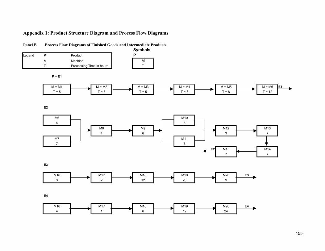
Appendix 1: Product Structure Diagram and Process Flow Diagrams
Panel B Process Flow Diagrams of Finished Goods and Intermediate Products Symbols
Legend P Product PM Machine MT Processing Time in hours. T
P = E1
M = M1 M = M2 M = M3 M = M4 M = M5 M = M6 E1T = 5 T = 8 T = 5 T = 8 T = 8 T = 12
E2
M6 M104 6
M8 M9 M12 M134 6 3 7
M7 M117 6
E2 M15 M147 7
E3
M16 M17 M18 M19 M20 E33 2 12 20 9
E4
M16 M17 M18 M19 M20 E44 1 6 12 24
155

Panel B Process Flow Diagrams of Finished Goods and Intermediate Products E5
M16 M17 M18 M19 M20 E53 2 22 2 8
E6M2345
M21 M22 E64 1
M2445
E7
M2348
M21 M22 E72 1
M2448
156

Panel B Process Flow Diagrams of Finished Goods and Intermediate Products
E8
M25 M26 M27 M28 M29 M30 E822 8 8 8 8 6
I1
M31 M32 I120 20
I2
M33 M34 M35 M36 I211 2 2 4
I3
M37 M38 I34 6
I4
M39 M40 I42 9
I5
M41 M42 I56 3
157

Panel B Process Flow Diagrams of Finished Goods and Intermediate Products
I6M47
4M43 M44 M45 M46 M48 I6
6 4 2 5 4M49
4
I7
M83 M84 M85 I76 4 2
I8
M57 M6210 12
M50 I836
M58 M6310 12
158

Panel B Process Flow Diagrams of Finished Goods and Intermediate Products I9
M57 M6212 16
M50 Filteration I920 2
M58 M6312 16
I10
M57 M628 16
M55 Filteration I1016 4
M58 M638 16
I11
M577
M52 I1120
M587
I12
M54 M56 Filteration M61 I1210 7 1 6
159

Panel B Process Flow Diagrams of Finished Goods and Intermediate Products
I13M5910
M52/M53 M51 Filteration M64 I1326 10 5 24
M6010
I14
M50 M51 M59 Filteration M64 I1410 12 10 2 10
I15M5712
M53 M50 M55 Filteration I1528 6 17 2
M5812
160

Panel B Process Flow Diagrams of Finished Goods and Intermediate Products I16 I17 I18
M59 M59 M599 9 8
M50/M51 I16 M50 I17 M50 I1820 17 17
M60 M60 M609 9 8
I19
M57 M61/M638 30
M52/M53/M54 Filteration I1980 4
M58 M62/M648 30
I20
M54 M56 Filteration M61 I2018 8 2 12
161

Panel B Process Flow Diagrams of Finished Goods and Intermediate Products I21
M578
M55 M52 M54 M56 M62 I2120 6 13 6 12
M588
I22
M53 M59 M54 M56 Filteration M62 I2230 10 6 6 2 20
I23
M71 M68 M72 M57 Filteration M78 I236 8 8 8 1 10
I24
M66 M65 M51 M73 M66 Filteration I247 7 6 7 8 1
I25
M74 M76 Filteration M79 I258 7 1 7
162

Panel B Process Flow Diagrams of Finished Goods and Intermediate Products
I26
M652
M69 M74 M76 Filteration M79 I2618 7 15 1 14
I27M70
7M71 M67 M72 M75 Filteration I27
3 M68 6 11 10 211
I28
M67 M73 M77 M78 M79 I285 12 11 12 10
I29
M81 M82 I294 2
163
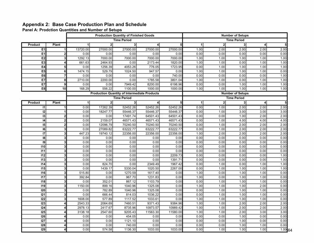
Appendix 2: Base Case Production Plan and Schedule Panel A: Prodction Quantities and Number of Setups
Time Period Time PeriodProduct Plant 1 2 3 4 5 1 2 3 4 5
E1 1 13720.00 27000.00 27000.00 27000.00 27000.00 1.00 2.00 2.00 2.00 2.00E1 2 0.00 0.00 0.00 0.00 0.00 0.00 0.00 0.00 0.00 0.00E2 3 1292.13 7000.00 7000.00 7000.00 7000.00 1.00 1.00 1.00 1.00 1.00E3 4 661.63 2464.93 0.00 2173.44 1820.00 1.00 1.00 0.00 1.00 1.00E4 5 0.00 1256.39 4053.26 776.05 1723.95 0.00 1.00 1.00 1.00 1.00E5 6 1474.15 529.79 1024.50 947.57 0.00 1.00 1.00 1.00 1.00 0.00E6 7 0.00 0.00 0.00 0.00 740.00 0.00 0.00 0.00 0.00 1.00E7 8 2710.00 2200.00 0.00 1785.58 3801.04 1.00 1.00 0.00 1.00 1.00E7 9 0.00 0.00 7949.42 8200.00 6198.96 0.00 0.00 1.00 1.00 1.00E8 10 168.29 556.22 1100.00 1000.00 1000.00 1.00 1.00 1.00 1.00 1.00
Time Period Time PeriodProduct Plant 1 2 3 4 5 1 2 3 4 5
I1 1 0.00 17262.39 52452.26 52452.26 52452.26 0.00 1.00 2.00 2.00 2.00I2 1 0.00 18247.77 55446.37 55446.37 55446.37 0.00 1.00 3.00 3.00 3.00I3 2 0.00 0.00 17491.74 64501.43 64501.43 0.00 0.00 1.00 2.00 2.00I4 2 0.00 2159.07 46571.43 46571.43 46571.43 0.00 1.00 4.00 4.00 4.00I5 2 0.00 12096.79 70240.50 70240.50 70240.50 0.00 1.00 2.00 2.00 2.00I6 3 0.00 27089.82 63222.77 63222.77 63222.77 0.00 1.00 2.00 2.00 2.00I7 3 447.23 19740.12 22356.00 22356.00 22356.00 1.00 2.00 2.00 2.00 2.00I8 3 0.00 0.00 0.00 0.00 0.00 0.00 0.00 0.00 0.00 0.00I9 3 0.00 0.00 0.00 0.00 0.00 0.00 0.00 0.00 0.00 0.00
I10 3 0.00 0.00 0.00 0.00 0.00 0.00 0.00 0.00 0.00 0.00I11 3 0.00 0.00 0.00 0.00 0.00 0.00 0.00 0.00 0.00 0.00I12 3 0.00 0.00 0.00 0.00 2209.73 0.00 0.00 0.00 0.00 1.00I13 3 0.00 0.00 0.00 0.00 1391.71 0.00 0.00 0.00 0.00 1.00I14 3 0.00 824.70 0.00 2349.49 1967.42 0.00 1.00 0.00 1.00 1.00I15 3 0.00 1439.17 5330.04 1020.50 2267.00 0.00 1.00 1.00 1.00 1.00I16 3 515.80 0.00 1270.59 1617.40 0.00 1.00 0.00 1.00 1.00 0.00I17 3 392.84 0.00 967.70 1231.83 0.00 1.00 0.00 1.00 1.00 0.00I18 3 0.00 352.01 867.12 1103.79 0.00 0.00 1.00 1.00 1.00 0.00I19 3 1150.00 899.16 1040.96 1325.08 0.00 1.00 1.00 1.00 2.00 0.00I20 3 0.00 782.89 1040.96 1325.08 0.00 0.00 1.00 1.00 1.00 0.00I21 3 0.00 666.44 814.03 1036.22 0.00 0.00 1.00 1.00 1.00 0.00I22 3 1608.00 577.89 1117.52 1033.61 0.00 1.00 1.00 1.00 1.00 0.00I23 4 2543.33 2064.69 7460.51 9371.43 9384.96 1.00 1.00 2.00 2.00 2.00I24 4 2978.13 2417.67 8735.96 10973.57 10989.42 1.00 1.00 2.00 2.00 2.00I25 4 3138.18 2547.60 9205.43 11563.30 11580.00 1.00 1.00 2.00 3.00 3.00I26 4 0.00 0.00 454.05 0.00 0.00 0.00 0.00 1.00 0.00 0.00I27 4 0.00 0.00 1121.10 0.00 0.00 0.00 0.00 1.00 0.00 0.00I28 4 0.00 0.00 740.00 0.00 0.00 0.00 0.00 1.00 1.00 0.00I29 4 0.00 574.58 1136.30 1033.00 1033.00 0.00 1.00 1.00 1.00 1.00
Number of SetupsProduction Quantity of Finished Goods
Number of SetupsProduction Quantity of Intermediate Products
164

Panel B: Inventory Levels of Products
Initial Inventory Time Period
0 1 2 3 4 5E1 13280.00 0.00 0.00 0.00 0.00 0.00E2 5707.87 0.00 0.00 0.00 0.00 0.00E3 0.00 661.63 2736.56 476.56 0.00 0.00E4 3861.35 3476.35 532.74 0.00 776.05 0.00E5 0.00 1474.15 967.93 92.43 0.00 0.00E6 510.00 510.00 510.00 510.00 510.00 0.00E7 0.00 0.00 0.00 14.42 0.00 0.00E8 875.49 543.78 0.00 0.00 0.00 0.00
Initial Inventory Time Period
0 1 2 3 4 5I1 0.00 0.00 0.00 0.00 0.00 0.00I2 5510.00 5510.00 0.00 0.00 0.00 0.00I3 50000.00 50000.00 47009.69 0.00 0.00 0.00I4 60000.00 60000.00 51199.38 34132.92 17066.46 0.00I5 18000.00 18000.00 0.00 0.00 0.00 0.00I6 30000.00 28735.23 0.00 0.00 0.00 0.00I7 12000.00 2615.88 0.00 0.00 0.00 0.00I8 9.48 9.48 9.48 9.48 9.48 9.48I9 2500.00 2500.00 2500.00 2500.00 2500.00 2500.00
I10 2500.00 2500.00 2500.00 2500.00 2500.00 2500.00I11 5010.00 5010.00 5010.00 5010.00 5010.00 3509.74I12 5664.00 5664.00 4673.85 1006.78 304.68 0.00I13 4516.00 4516.00 3568.42 3568.42 868.86 0.00I14 2555.11 1839.89 0.00 0.00 0.00 0.00I15 212.98 212.98 0.00 0.00 0.00 0.00I16 0.00 0.00 0.00 0.00 0.00 0.00I17 0.00 392.84 0.00 0.00 0.00 0.00I18 300.14 300.14 0.00 0.00 0.00 0.00I19 1144.86 233.40 391.71 0.00 0.00 0.00I20 1266.27 116.27 0.00 0.00 0.00 0.00I21 936.00 36.70 0.00 0.00 0.00 0.00I22 0.00 0.00 0.00 0.00 0.00 0.00I23 0.00 0.00 0.00 0.00 0.00 0.00I24 0.00 0.00 0.00 0.00 0.00 0.00I25 0.00 0.00 0.00 0.00 0.00 0.00I26 0.00 0.00 0.00 0.00 0.00 0.00I27 0.00 0.00 0.00 0.00 0.00 0.00I28 0.00 0.00 0.00 740.00 740.00 0.00I29 173.84 0.00 0.00 0.00 0.00 0.00
Inventory of Finished Goods
Inventory of Intermediate Products
165

Panel C: Capacity Utilized (in hours) in Dedicated PlantsTime Period
Plant 1 2 3 4 51 457.63 684.00 684.00 684.00 478.772 0.00 219.63 502.56 502.56 502.564 341.07 281.40 0.00 232.91 468.725 0.00 0.00 636.11 655.40 684.006 0.00 213.15 641.43 641.43 641.438 0.00 188.48 572.46 572.46 572.469 28.50 415.06 464.76 464.76 464.76
10 325.84 642.00 642.00 642.00 642.0011 76.98 311.00 311.00 311.00 311.0012 0.00 0.00 175.92 647.01 647.0113 0.00 38.23 684.00 684.00 684.0014 0.00 72.39 328.96 328.96 328.9615 72.63 184.75 341.90 313.00 313.0016 0.00 131.89 213.90 198.82 198.82
Available Capacity : 684 hours in a month
166

Panel D: Capacity utilized (in hours) of Machines in Flexible PlantsTime Period
Machine Plant 1 2 3 4 5M50 3 44.03 171.64 247.32 419.28 247.31M51 3 35.21 105.25 69.18 340.26 292.41M52 3 412.00 460.45 534.50 312.71 161.90M53 3 345.23 283.07 689.47 720.00 220.32M54 3 320.40 374.27 529.90 586.47 165.31M55 3 12.00 243.86 453.27 300.40 131.05M56 3 320.40 369.45 523.73 578.62 120.51M57 3 393.33 518.42 720.00 720.00 99.57M58 3 0.00 0.00 0.00 0.00 0.00M59 3 367.46 254.40 366.80 595.23 260.11M60 3 0.00 0.00 0.00 0.00 0.00M61 3 399.03 418.93 497.09 638.22 105.58M62 3 327.88 302.11 457.61 492.64 0.00M63 3 0.00 0.00 0.00 0.00 0.00M64 3 0.00 91.71 0.00 216.90 336.51M65 7 171.12 143.43 505.73 590.09 590.88M66 7 171.12 143.43 479.56 590.09 590.88M67 7 150.27 126.51 470.52 537.28 513.95M68 7 147.17 123.23 498.69 508.57 509.25M69 7 0.00 0.00 92.01 0.00 0.00M70 7 0.00 0.00 63.24 0.00 0.00M71 7 116.65 98.46 364.32 396.11 396.63M72 7 147.17 123.23 498.69 508.57 509.25M73 7 171.12 143.43 570.90 614.09 590.88M74 7 164.91 135.38 523.33 602.16 603.00M75 7 147.17 123.23 493.08 508.57 509.25M76 7 142.94 117.55 491.58 521.22 521.94M77 7 171.12 143.43 564.98 614.09 590.88M78 7 198.03 164.53 653.58 720.00 696.95M79 7 142.94 117.55 567.74 545.22 521.94M80 7 171.12 143.43 479.56 590.09 590.88
Available Capacity : 720 hours in a month
167
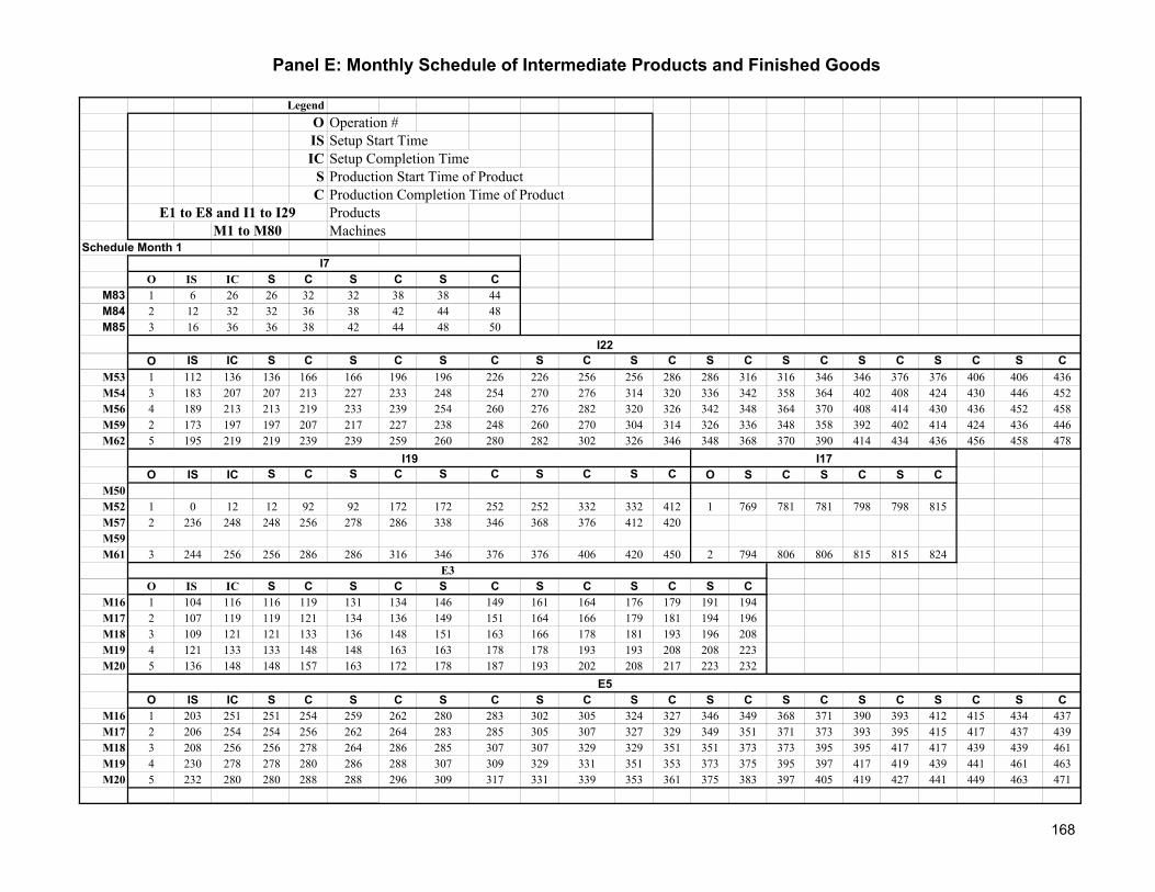
Panel E: Monthly Schedule of Intermediate Products and Finished Goods
LegendO Operation #IS Setup Start TimeIC Setup Completion Time
S Production Start Time of ProductC Production Completion Time of Product
ProductsM1 to M80 Machines
Schedule Month 1
O IS IC S C S C S CM83 1 6 26 26 32 32 38 38 44M84 2 12 32 32 36 38 42 44 48M85 3 16 36 36 38 42 44 48 50
O IS IC S C S C S C S C S C S C S C S C S C S CM53 1 112 136 136 166 166 196 196 226 226 256 256 286 286 316 316 346 346 376 376 406 406 436M54 3 183 207 207 213 227 233 248 254 270 276 314 320 336 342 358 364 402 408 424 430 446 452M56 4 189 213 213 219 233 239 254 260 276 282 320 326 342 348 364 370 408 414 430 436 452 458M59 2 173 197 197 207 217 227 238 248 260 270 304 314 326 336 348 358 392 402 414 424 436 446M62 5 195 219 219 239 239 259 260 280 282 302 326 346 348 368 370 390 414 434 436 456 458 478
O IS IC S C S C S C S C S C O S C S C S CM50M52 1 0 12 12 92 92 172 172 252 252 332 332 412 1 769 781 781 798 798 815M57 2 236 248 248 256 278 286 338 346 368 376 412 420M59M61 3 244 256 256 286 286 316 346 376 376 406 420 450 2 794 806 806 815 815 824
O IS IC S C S C S C S C S C S CM16 1 104 116 116 119 131 134 146 149 161 164 176 179 191 194M17 2 107 119 119 121 134 136 149 151 164 166 179 181 194 196M18 3 109 121 121 133 136 148 151 163 166 178 181 193 196 208M19 4 121 133 133 148 148 163 163 178 178 193 193 208 208 223M20 5 136 148 148 157 163 172 178 187 193 202 208 217 223 232
O IS IC S C S C S C S C S C S C S C S C S C S CM16 1 203 251 251 254 259 262 280 283 302 305 324 327 346 349 368 371 390 393 412 415 434 437M17 2 206 254 254 256 262 264 283 285 305 307 327 329 349 351 371 373 393 395 415 417 437 439M18 3 208 256 256 278 264 286 285 307 307 329 329 351 351 373 373 395 395 417 417 439 439 461M19 4 230 278 278 280 286 288 307 309 329 331 351 353 373 375 395 397 417 419 439 441 461 463M20 5 232 280 280 288 288 296 309 317 331 339 353 361 375 383 397 405 419 427 441 449 463 471
E3
E5
I22
E1 to E8 and I1 to I29
I7
I19 I17
168

Panel E: Monthly Schedule of Intermediate Products and Finished Goods
O C S C S CM16 1 481 500 503 522 525M17 2 483 503 505 525 527M18 3 505 505 527 527 549M19 4 507 527 529 549 551M20 5 515 529 537 551 559
Schedule Month 2
O IS IC S C S C S C S C S C S C S C S C S C S CM31 1 424 430 430 450 450 470 470 490 490 510 510 530 530 550 550 570 570 590 590 610 610 630M32 2 444 450 450 470 470 490 490 510 510 530 530 550 550 570 570 590 590 610 610 630 630 650
O IS IC S C S C S C S C S C S C S C S C S C S CM33 1 130 136 136 147 147 158 158 169 169 180 180 191 191 202 202 213 213 224 224 235 235 246M34 2 141 147 147 149 158 160 169 171 180 182 191 193 202 204 213 215 224 226 235 237 246 248M35 3 143 149 149 151 160 162 171 173 182 184 193 195 204 206 215 217 226 228 237 239 248 250M36 4 145 151 151 155 162 166 173 177 184 188 195 199 206 210 217 221 228 232 239 243 250 254
O IS IC S C S C S CM39 1 683 691 691 693 700 702 709 711M40 2 685 693 693 702 702 711 711 720
O IS IC S C S C S C S C S C S C S C S C S C S CM41 1 621 645 645 651 651 657 657 663 663 669 669 675 675 681 681 687 687 693 693 699 699 705M42 2 627 651 651 654 657 660 663 666 669 672 675 678 681 684 687 690 693 696 699 702 705 708
O IS IC S C S C S C S C S C S C S C S C S C S CM43 1 315 345 345 351 351 357 357 363 363 369 369 375 375 381 381 387 387 393 393 399 399 405M44 2 321 351 351 355 357 361 363 367 369 373 375 379 381 385 387 391 393 397 399 403 405 409M45 3 325 355 355 357 361 363 367 369 373 375 379 381 385 387 391 393 397 399 403 405 409 411M46 4 327 357 357 362 363 368 369 374 375 380 381 386 387 392 393 398 399 404 405 410 411 416M47 5 332 362 362 366 380 384 398 402 416 420M48 5 338 368 368 372 386 390 404 408M49 5 344 374 374 378 392 396 410 414
E5
I5
I6
I1
I2
I4
169

Panel E: Monthly Schedule of Intermediate Products and Finished Goods
O IS IC S C S C S C S C S C S C S C S C S C S CM83 1 0 20 20 26 26 32 32 38 38 44 44 50 50 56 56 62 62 68 68 74 74 80M84 2 6 26 26 30 32 36 38 42 44 48 50 54 56 60 62 66 68 72 74 78 80 84M85 3 8 28 28 30 36 38 42 44 48 50 54 56 60 62 66 68 72 74 78 80 84 86
O IS IC S C S C S C S CM81 1 654 702 702 706 706 710 710 714 714 718M82 2 658 706 706 708 710 712 714 716 718 720
O IS IC S C S C S C S C S C S C S C S CM50 1 260 284 284 294 299 309 314 324 329 339 344 354 359 369 374 384 389 399M51 2 270 294 294 306 309 321 324 336 339 351 354 366 369 381 384 396 399 411M59 3 282 306 306 316 321 331 336 346 351 361 366 376 381 391 396 406 411 421M64 4 292 316 316 326 331 341 346 356 361 371 376 386 391 401 406 416 421 431
O IS IC S C S C S C S C S CM50 2 425 449 449 455 466 472 483 489 500 506 517 523M53 1 322 346 346 374 374 402 402 430 430 458 458 486M55 3 431 455 455 472 472 489 489 506 506 523 523 540M57 4 468 492 492 504 504 516 516 528 528 540 540 552
O IS IC S C S CM50 1 202 214 214 231 231 260M59 2 230 242 242 250 484 504M60 3 238 250 250 258 492 512
O IS IC S C S C S C S CM52 1 208 220 220 300 300 380 380 460 679 771M57 2 432 444 444 452 452 460 460 468 759 779M61 3 498 510 510 540 540 570 570 600 767 809
O IS IC S C S C S C S C S C S CM54 1 116 128 128 146 240 258 258 276 312 330 500 530 530 548M56 2 146 158 158 166 268 276 276 284 342 350 528 548 548 556M61 3 196 208 208 220 276 288 288 300 368 380 655 679 679 691
I14
I18
I15
I19
I7
I29
I20
170

Panel E: Monthly Schedule of Intermediate Products and Finished Goods
O IS IC S C S C S C S C S CM52 3 140 164 164 170 170 176 190 196 196 202 202 208M54 4 146 170 170 183 183 196 227 240 330 343 343 356M55 1 70 94 94 114 114 134 134 154 154 174 174 194M56 5 166 190 190 196 196 202 262 268 350 356 356 362M57 2 130 154 154 162 162 170 178 186 186 194 194 202M62 6 172 196 196 208 208 220 288 300 356 368 368 380
O IS IC S C S C S C S CM53 1 486 510 510 540 540 570 570 600 600 630M54 3 550 574 574 580 596 602 618 624 640 646M56 4 556 580 580 586 602 608 624 630 646 652M59 2 540 564 564 574 586 596 608 618 630 640M62 5 562 586 586 606 608 628 630 650 652 672
O IS IC S C S C S C S C S C S C S C S C S C S CM16 1 89 101 101 104 116 119 131 134 146 149 161 164 176 179 191 194 206 209 221 224 236 239M17 2 92 104 104 106 119 121 134 136 149 151 164 166 179 181 194 196 209 211 224 226 239 241M18 3 94 106 106 118 121 133 136 148 151 163 166 178 181 193 196 208 211 223 226 238 241 253M19 4 106 118 118 133 133 148 148 163 163 178 178 193 193 208 208 223 223 238 238 253 253 268M20 5 124 136 136 145 151 160 166 175 181 190 196 205 211 220 226 235 241 250 256 265 271 280
O S C S C S C S C S C S C S C S C S C S C S CM16 1 266 269 281 284 296 299 311 314 326 329 341 344 356 359 371 374 386 389 401 404 416 419M17 2 269 271 284 286 299 301 314 316 329 331 344 346 359 361 374 376 389 391 404 406 419 421M18 3 271 283 286 298 301 313 316 328 331 343 346 358 361 373 376 388 391 403 406 418 421 433M19 4 283 298 298 313 313 328 328 343 343 358 358 373 373 388 388 403 403 418 418 433 433 448M20 5 301 310 316 325 331 340 346 355 361 370 376 385 391 400 406 415 421 430 436 445 451 460
O IS IC S C S C S C S C S C S C S C S C S C S CM16 1 450 498 498 502 504 508 510 514 516 520 522 526 528 532 534 538 540 544 546 550 552 556M17 2 451 499 499 503 508 509 514 515 520 521 526 527 532 533 538 539 544 545 550 551 556 557M18 3 455 503 503 509 509 515 515 521 521 527 527 533 533 539 539 545 545 551 551 557 557 563M19 4 463 511 511 523 523 535 535 547 547 559 559 571 571 583 583 595 595 607 607 619 619 631M20 5 475 523 523 535 535 547 547 559 559 571 571 583 583 595 595 607 607 619 619 631 631 643
E4
I21
I22
E3
E3
171

Panel E: Monthly Schedule of Intermediate Products and Finished Goods
O IS IC S C S C S C S C S CM16 1 558 606 606 609 628 631 650 653 672 675 694 697M17 2 561 609 609 611 631 633 653 655 675 677 697 699M18 3 563 611 611 633 633 655 655 677 677 699 699 721M19 4 641 689 689 691 697 699 705 707 713 715 721 723M20 5 643 691 691 699 699 707 707 715 715 723 723 731
Schedule Month 3
O IS IC S C S C S C S C S C S C S C S C S CM31 1 18 24 24 44 44 64 64 84 84 104 104 124 124 144 144 164 164 184 184 204M32 2 38 44 44 64 64 84 84 104 104 124 124 144 144 164 164 184 184 204 204 224
O S C S C S C S C S C S CM31 1 204 224 224 244 244 264 264 284 284 304 304 324M32 2 224 244 244 264 264 284 284 304 304 324 324 344
O IS IC S C S C S C S C S C S C S C S C S C S CM33 1 0 6 6 17 17 28 28 39 39 50 50 61 61 72 72 83 83 94 94 105 105 116M34 2 11 17 17 19 28 30 39 41 50 52 61 63 72 74 83 85 94 96 105 107 116 118M35 3 13 19 19 21 30 32 41 43 52 54 63 65 74 76 85 87 96 98 107 109 118 120M36 4 17 23 21 25 32 36 43 47 50 54 61 65 71 75 82 86 93 97 104 108 120 124
O IS IC S C S C S C S C S C S C S C S C S C S CM37 1 625 626 626 630 632 636 638 642 644 648 650 654 656 660 662 666 668 672 674 678 680 684M38 2 629 630 630 636 636 642 642 648 648 654 654 660 660 666 666 672 672 678 678 684 684 690
S C S C S C S C S CM37 686 690 692 696 698 702 704 708 710 714M38 690 696 696 702 702 708 708 714 714 720
O IS IC S C S C S C S C S C S C S C S C S C S CM39 1 182 190 190 192 199 201 208 210 217 219 226 228 235 237 244 246 253 255 262 264 271 273M40 2 184 192 192 201 201 210 210 219 219 228 228 237 237 246 246 255 255 264 264 273 273 282
E5
I1
I1
I2
I3
I4
172

Panel E: Monthly Schedule of Intermediate Products and Finished Goods
O IS IC S C S C S C S C S C S C S C S C S C S CM41 1 255 279 279 285 285 291 291 297 297 303 303 309 309 315 315 321 321 327 327 333 333 339M42 2 261 285 285 288 291 294 297 300 303 306 309 312 315 318 321 324 327 330 333 336 339 342
O IS IC S C S C S C S C S C S C S C S C S C S CM43 1 0 30 30 36 36 42 42 48 48 54 54 60 60 66 66 72 72 78 78 84 84 90M44 2 6 36 36 40 42 46 48 52 54 58 60 64 66 70 72 76 78 82 84 88 90 94M45 3 10 40 40 42 46 48 52 54 58 60 64 66 70 72 76 78 82 84 88 90 94 96M46 4 12 32 42 47 48 53 54 59 60 65 66 71 72 77 78 83 84 89 90 95 96 101M47 5 17 47 47 51 65 69 83 87 101 105M48 5 23 53 53 57 71 75 89 93M49 5 29 59 59 63 77 81 95 99
O IS IC S C S C S C S C S C S C S C S C S CM83 1 25 31 31 37 37 43 43 49 49 55 55 61 61 67 67 73 73 79 79 85M84 2 31 35 37 41 43 47 49 53 55 59 61 65 67 71 73 77 79 83 85 89M85 3 33 35 41 43 47 49 53 55 59 61 65 67 71 73 77 79 83 85 89 91
O IS IC S C S C S C S C S C S C S C S CM81 1 638 686 686 690 690 694 694 698 698 702 702 706 706 710 710 714 714 718M82 2 642 690 690 692 694 696 698 700 702 704 706 708 710 712 714 716 718 720
O IS IC S C S C S C S C S C S C S CM50 2 185 209 209 215 233 239 257 263 281 287 305 311 329 335 353 359M53 1 0 24 24 52 52 80 80 108 108 136 136 164 164 192 192 220M55 3 191 215 215 232 239 256 263 280 287 304 311 328 335 352 359 376M57 4 208 232 232 244 256 268 280 292 304 316 328 340 352 364 376 388
O IS IC S C S C S CM50 1 582 594 594 611 611 628 628 645M59 2 636 648 648 657 662 671 671 680
O IS IC S C S C S CM50 1 645 657 657 674 674 691 691 708M59 2 680 692 692 700 700 708 708 716M60 3 688 700 700 708 708 716 716 724
I6
I7
I29
I15
I18
I5
I17
173
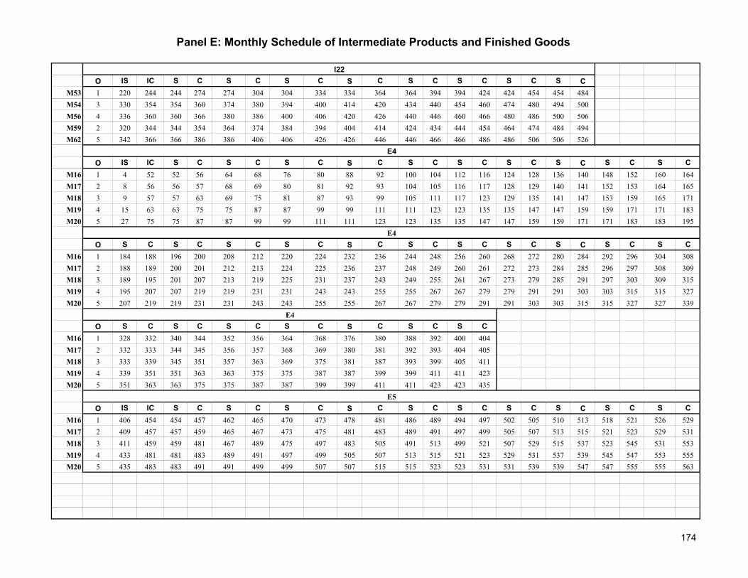
Panel E: Monthly Schedule of Intermediate Products and Finished Goods
O IS IC S C S C S C S C S C S C S C S CM53 1 220 244 244 274 274 304 304 334 334 364 364 394 394 424 424 454 454 484M54 3 330 354 354 360 374 380 394 400 414 420 434 440 454 460 474 480 494 500M56 4 336 360 360 366 380 386 400 406 420 426 440 446 460 466 480 486 500 506M59 2 320 344 344 354 364 374 384 394 404 414 424 434 444 454 464 474 484 494M62 5 342 366 366 386 386 406 406 426 426 446 446 466 466 486 486 506 506 526
O IS IC S C S C S C S C S C S C S C S C S C S CM16 1 4 52 52 56 64 68 76 80 88 92 100 104 112 116 124 128 136 140 148 152 160 164M17 2 8 56 56 57 68 69 80 81 92 93 104 105 116 117 128 129 140 141 152 153 164 165M18 3 9 57 57 63 69 75 81 87 93 99 105 111 117 123 129 135 141 147 153 159 165 171M19 4 15 63 63 75 75 87 87 99 99 111 111 123 123 135 135 147 147 159 159 171 171 183M20 5 27 75 75 87 87 99 99 111 111 123 123 135 135 147 147 159 159 171 171 183 183 195
O S C S C S C S C S C S C S C S C S C S C S CM16 1 184 188 196 200 208 212 220 224 232 236 244 248 256 260 268 272 280 284 292 296 304 308M17 2 188 189 200 201 212 213 224 225 236 237 248 249 260 261 272 273 284 285 296 297 308 309M18 3 189 195 201 207 213 219 225 231 237 243 249 255 261 267 273 279 285 291 297 303 309 315M19 4 195 207 207 219 219 231 231 243 243 255 255 267 267 279 279 291 291 303 303 315 315 327M20 5 207 219 219 231 231 243 243 255 255 267 267 279 279 291 291 303 303 315 315 327 327 339
O S C S C S C S C S C S C S CM16 1 328 332 340 344 352 356 364 368 376 380 388 392 400 404M17 2 332 333 344 345 356 357 368 369 380 381 392 393 404 405M18 3 333 339 345 351 357 363 369 375 381 387 393 399 405 411M19 4 339 351 351 363 363 375 375 387 387 399 399 411 411 423M20 5 351 363 363 375 375 387 387 399 399 411 411 423 423 435
O IS IC S C S C S C S C S C S C S C S C S C S CM16 1 406 454 454 457 462 465 470 473 478 481 486 489 494 497 502 505 510 513 518 521 526 529M17 2 409 457 457 459 465 467 473 475 481 483 489 491 497 499 505 507 513 515 521 523 529 531M18 3 411 459 459 481 467 489 475 497 483 505 491 513 499 521 507 529 515 537 523 545 531 553M19 4 433 481 481 483 489 491 497 499 505 507 513 515 521 523 529 531 537 539 545 547 553 555M20 5 435 483 483 491 491 499 499 507 507 515 515 523 523 531 531 539 539 547 547 555 555 563
E4
E5
I22
E4
E4
174

Panel E: Monthly Schedule of Intermediate Products and Finished Goods
Schedule Month 4
O IS IC S C S C S C S C S C S C S C S C S CM31 1 28 34 34 54 54 74 74 94 94 114 114 134 134 154 154 174 174 194 194 214M32 2 58 64 64 74 74 94 94 114 114 134 134 154 154 174 174 194 194 214 214 234
O S C S C S C S C S C S CM31 1 214 234 234 254 254 274 274 294 294 314 314 334M32 2 234 254 254 274 274 294 294 314 314 334 334 354
O IS IC S C S C S C S C S C S C S C S C S C S CM33 1 10 16 16 27 27 38 38 49 49 60 60 71 71 82 82 93 93 104 104 115 115 126M34 2 21 27 27 29 38 40 49 51 60 62 71 73 82 84 93 95 104 106 115 117 126 128M35 3 23 29 29 31 40 42 51 53 62 64 73 75 84 86 95 97 106 108 117 119 128 130M36 4 27 33 31 35 42 46 53 57 60 64 71 75 81 85 92 96 103 107 114 118 130 134
O IS IC S C S C S C S C S C S C S C S C S C S CM37 1 384 385 385 389 391 395 397 401 403 407 409 413 415 419 421 425 427 431 433 437 439 443M38 2 388 389 389 395 395 401 401 407 407 413 413 419 419 425 425 431 431 437 437 443 443 449
O IS IC S C S C S C S C S C S C S C S C S C S CM39 1 192 200 200 202 209 211 218 220 227 229 236 238 245 247 254 256 263 265 272 274 281 28.3M40 2 194 202 202 211 211 220 220 229 229 238 238 247 247 256 256 265 265 274 274 283 283 292
O IS IC S C S C S C S C S C S C S C S C S C S CM41 1 265 289 289 295 295 301 301 307 317 313 313 319 319 325 325 331 331 337 337 343 343 349M42 2 271 305 295 298 301 304 307 310 313 316 319 322 325 328 331 334 337 340 343 346 349 352
O IS IC S C S C S C S C S C S C S C S C S C S CM43 1 10 40 40 46 46 52 52 58 58 64 64 70 70 76 76 82 82 88 88 94 94 100M44 2 16 46 46 50 52 56 58 62 64 68 70 74 76 80 82 86 88 92 94 98 100 104M45 3 20 50 50 52 56 58 62 64 68 70 74 76 80 82 86 88 92 94 98 100 104 106M46 4 22 42 52 57 58 63 64 69 70 75 76 81 82 87 88 93 94 99 100 105 106 111M47 5 27 57 57 61 75 79 93 97 111 115M48 5 33 63 63 67 81 85 99 103M49 5 39 69 69 73 87 91 105 109
I6
I1
I1
I2
I3
I4
I5
175

Panel E: Monthly Schedule of Intermediate Products and Finished Goods
O IS IC S C S C S C S C S C S C S C S C S CM83 1 30 36 36 42 42 48 48 54 54 60 60 66 66 72 72 78 78 84 84 90M84 2 36 40 42 46 48 52 54 58 60 64 66 70 72 76 78 82 84 88 90 94M85 3 38 40 46 48 52 54 58 60 64 66 70 72 76 78 82 84 88 90 94 96
O IS IC S C S C S C S C S C S C S CM81 1 642 690 690 694 694 698 698 702 702 706 706 710 710 714 714 718M82 2 646 694 694 696 698 700 702 704 706 708 710 712 714 716 718 720
O IS IC S C S C S C S C S C S C S C S C S C S CM50 1 195 219 219 229 231 241 243 253 255 265 267 277 279 289 291 301 303 313 315 325 327 337M51 2 205 229 229 241 241 253 253 265 265 277 277 289 289 301 301 313 313 325 325 337 337 349M59 3 217 241 241 251 253 263 265 275 277 287 289 299 301 311 313 323 325 335 337 347 349 359M64 4 227 251 251 261 263 273 275 285 287 297 299 309 311 321 323 333 335 345 347 357 359 369
O S C S C S C S C S C S C S C S C S CM50 1 351 361 363 373 375 385 387 397 399 409 411 421 423 433 435 445 447 457M51 2 361 373 373 385 385 397 397 409 409 421 421 433 433 445 445 457 457 469M59 3 373 383 385 395 397 407 409 419 421 431 433 443 445 455 457 467 469 479M64 4 383 393 395 405 407 417 419 429 431 441 443 453 455 465 467 477 479 489
O IS IC S C S C S CM50 2 480 504 504 510 521 527 538 544M53 1 403 427 427 455 455 483 483 511M55 3 486 510 510 527 527 544 544 561M57 4 513 537 537 549 549 561 561 573
O IS IC S C S C S C S CM50 1 835 847 847 867 867 899 899 919 919 939M59 2 888 900 900 909 909 930 930 939 939 948
O IS IC S CM50 1 931 943 943 960M59 2 948 960 960 969
I14
I14
I16
I17
I29
I7
I15
176

Panel E: Monthly Schedule of Intermediate Products and Finished Goods
O IS IC S C S C S C S C S CM50 1 0 12 12 29 92 109 144 161 161 178 178 195M59 2 17 25 25 37 109 117 193 201 201 209 209 217M60 3 25 37 37 45 117 125 219 227 379 387 417 425
O IS IC S C S C S C S C S C S C S CM52 1 93 105 105 185 185 265 265 345 345 425 425 505 505 597 597 677M57 2 469 481 481 489 489 497 497 505 505 513 605 613 635 655 677 685M61 3 481 493 493 523 523 553 553 583 583 613 613 643 643 685 685 715
O IS IC S C S C S C S C S C S C S C S C S C S CM54 1 33 45 45 63 63 81 125 143 143 161 227 245 285 303 303 321 387 405 407 425 425 443M56 2 61 73 73 81 81 89 153 161 161 169 245 253 313 321 321 329 405 413 437 445 445 453M61 3 69 81 81 93 93 105 161 173 173 185 253 265 321 333 333 345 413 425 445 457 457 469
O IS IC S C S C S CM52 3 870 894 894 900 900 906 906 912M54 4 876 900 900 913 913 926 926 939M55 1 814 838 838 858 858 878 878 898M56 5 903 927 927 933 933 939 939 945M57 2 858 882 882 890 890 898 898 906M62 6 909 933 933 945 945 957 957 969
O IS IC S C S C S C S C S C S C S CM53 1 511 535 535 565 565 595 595 625 625 655 655 685 685 715 715 745M54 3 577 601 601 607 623 629 645 651 667 673 711 717 733 739 755 761M56 4 583 607 607 613 629 635 651 657 673 679 717 723 739 745 761 767M59 2 567 591 591 601 613 623 635 645 657 667 701 711 723 733 745 755M62 5 589 613 613 633 635 655 657 677 679 699 723 743 745 765 767 787
O IS IC S C S C S C S C S C S C S C S C S C S CM16 1 249 261 261 264 273 276 285 288 297 300 309 312 321 324 333 336 345 348 357 360 369 372M17 2 252 264 264 266 276 278 288 290 300 302 312 314 324 326 336 338 348 350 360 362 372 374M18 3 254 266 266 278 278 290 290 302 302 314 314 326 326 338 338 350 350 362 362 374 374 386M19 4 266 278 278 293 293 308 308 323 323 338 338 353 353 368 368 383 383 398 398 413 413 428M20 5 284 296 296 305 311 320 326 335 341 350 356 365 371 380 386 395 401 410 416 425 431 440
I19
I18
E3
I22
I21
I20
177
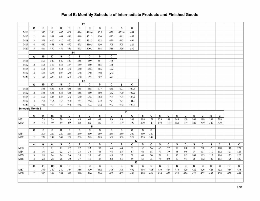
Panel E: Monthly Schedule of Intermediate Products and Finished Goods
O S C S C S C S C S CM16 1 393 396 405 408 414 419.4 425 430 435.6 441M17 2 396 398 408 410 419 421.2 430 432 441 443M18 3 398 410 410 422 421 435.2 432 450 443 464M19 4 443 458 458 473 475 489.5 450 508 508 526M20 5 461 470 476 485 493 500.3 508 516 526 532
O IS IC S C S C S CM16 1 501 549 549 553 555 559 561 565M17 2 505 553 553 554 559 560 565 566M18 3 506 554 554 560 560 566 566 572M19 4 578 626 626 638 638 650 650 662M20 5 590 638 638 650 650 662 662 674
O IS IC S C S C S C S CM16 1 585 633 633 636 655 658 677 680 691 700.4M17 2 588 636 636 638 658 660 680 682 700 702.2M18 3 590 638 638 660 660 682 682 704 704 728.2M19 4 708 756 756 758 764 766 772 774 774 781.6M20 5 710 758 758 766 766 774 774 782 782 790.8
Schedule Month 5
O IS IC S C S C S C S C S C S C S C S C S CM31 1 23 29 29 49 49 69 69 89 89 109 109 129 129 149 149 169 169 189 189 209M32 2 43 49 49 69 69 89 89 109 109 129 129 149 149 169 169 189 189 209 209 229
O S C S C S C S C S C S CM31 1 209 229 229 249 249 269 269 289 289 309 309 329M32 2 229 249 249 269 269 289 289 309 309 329 329 349
O IS IC S C S C S C S C S C S C S C S C S C S CM33 1 5 11 11 22 22 33 33 44 44 55 55 66 66 77 77 88 88 99 99 110 110 121M34 2 16 22 22 24 33 35 44 46 55 57 66 68 77 79 88 90 94 101 110 112 121 123M35 3 18 24 24 26 35 37 46 48 57 59 68 70 79 81 93 92 101 103 112 114 123 125M36 4 22 28 26 30 37 41 48 52 55 59 66 75 76 80 87 91 98 102 109 113 125 129
O IS IC S C S C S C S C S C S C S C S C S C S CM37 1 379 380 380 384 386 390 392 396 398 402 404 408 410 414 416 420 422 426 428 432 434 438M38 2 383 384 384 390 390 396 396 402 402 408 408 414 414 420 420 426 426 432 432 438 438 444
E5
I3
E4
E3
I1
I1
I2
178

Panel E: Monthly Schedule of Intermediate Products and Finished Goods
O IS IC S C S C S C S C S C S C S C S C S C S CM39 1 187 195 195 197 204 206 213 215 222 224 231 233 240 242 249 251 258 260 267 269 276 278M40 2 189 197 197 206 206 215 215 224 224 233 233 242 242 251 251 260 260 269 269 278 278 287
O IS IC S C S C S C S C S C S C S C S C S C S CM41 1 260 284 284 290 290 296 296 302 302 308 308 314 314 320 320 326 326 332 332 338 338 344M42 2 266 295 290 293 296 299 302 305 308 311 314 317 320 323 326 329 332 335 338 341 344 347
O IS IC S C S C S C S C S C S C S C S C S C S CM43 1 5 35 35 41 41 47 47 53 53 59 59 65 65 71 71 77 77 83 83 89 89 95M44 2 11 41 41 45 47 51 53 57 59 63 65 69 71 75 77 81 83 87 89 93 95 99M45 3 15 45 45 47 51 53 57 59 63 65 69 71 75 77 81 83 87 89 93 95 99 101M46 4 17 37 47 52 53 58 59 64 65 70 71 76 77 82 83 88 89 94 95 100 101 106M47 5 22 52 52 56 70 74 88 92 106 110M48 5 28 58 58 62 76 80 94 98M49 5 34 64 64 68 82 86 100 104
O IS IC S C S C S C S C S C S C S C S C S CM83 1 40 46 46 52 52 58 58 64 64 70 70 76 76 82 82 88 88 94 94 95M84 2 46 50 52 56 58 62 64 68 70 74 76 80 82 86 88 92 94 98 100 99M85 3 48 50 56 58 62 64 68 70 74 76 80 82 86 88 92 94 98 100 104 101
O IS IC S C S C S C S C S C S C S CM81 1 642 690 690 694 694 698 698 702 702 706 706 710 710 714 714 718M82 2 646 694 694 696 698 700 702 704 706 708 710 712 714 716 718 720
O IS IC S C S C S C S C S C S C S C S CM50 1 0 24 24 34 39 49 54 64 69 79 84 94 99 109 114 124 129 139M51 2 10 34 34 46 49 61 64 76 79 91 94 106 109 121 124 136 139 151M59 3 22 46 46 56 61 71 76 86 91 101 106 116 121 131 136 146 151 161M64 4 32 56 56 66 71 81 86 96 101 111 116 126 131 141 146 156 161 171
O IS IC S C S C S C S C S CM50 2 316 340 340 346 364 370 388 394 412 418 436 442M53 1 264 288 288 316 316 344 344 372 372 400 400 428M55 3 322 346 346 363 370 387 394 411 418 435 442 459M57 4 339 363 363 375 387 399 411 423 435 447 459 471
I15
I14
I4
I5
I6
I7
I29
179

Appendix 3: Sensitivity Analysis on Production Planning and Scheduling ResultsCase 1- Base Case
Production Quantity of Finished GoodsTime Period Time Period
Product Plant 1 2 3 4 5 1 2 3 4 5E1 1 13720.00 27000.00 27000.00 27000.00 27000.00 1 2 2 2 2E1 2 0.00 0.00 0.00 0.00 0.00 0 0 0 0 0E2 3 1292.13 7000.00 7000.00 7000.00 7000.00 1 1 1 1 1E3 4 661.63 2464.93 0.00 2173.44 1820.00 1 1 0 1 1E4 5 0.00 1256.39 4053.26 776.05 1723.95 0 1 1 1 1E5 6 1474.15 529.79 1024.50 947.57 0.00 1 1 1 1 0E6 7 0.00 0.00 0.00 0.00 740.00 0 0 0 0 1E7 8 2710.00 2200.00 0.00 1785.58 3801.04 1 1 0 1 1E7 9 0.00 0.00 7949.42 8200.00 6198.96 0 0 1 1 1E8 10 168.29 556.22 1100.00 1000.00 1000.00 1 1 1 1 1
Production Quantity of Intermediate GoodsProduction Quantity of Intermediate Products
Time Period Time PeriodProduct Plant 1 2 3 4 5 1 2 3 4 5
I1 1 0.00 17262.39 52452.26 52452.26 52452.26 0 1 2 2 2I2 1 0.00 18247.77 55446.37 55446.37 55446.37 0 1 3 3 3I3 2 0.00 0.00 17491.74 64501.43 64501.43 0 0 1 2 2I4 2 0.00 2159.07 46571.43 46571.43 46571.43 0 1 4 4 4I5 2 0.00 12096.79 70240.50 70240.50 70240.50 0 1 2 2 2I6 3 0.00 27089.82 63222.77 63222.77 63222.77 0 1 2 2 2I7 3 447.23 19740.12 22356.00 22356.00 22356.00 1 2 2 2 2I8 3 0.00 0.00 0.00 0.00 0.00 0 0 0 0 0I9 3 0.00 0.00 0.00 0.00 0.00 0 0 0 0 0
I10 3 0.00 0.00 0.00 0.00 0.00 0 0 0 0 0I11 3 0.00 0.00 0.00 0.00 0.00 0 0 0 0 0I12 3 0.00 0.00 0.00 0.00 2209.73 0 0 0 0 1I13 3 0.00 0.00 0.00 0.00 1391.71 0 0 0 0 1I14 3 0.00 824.70 0.00 2349.49 1967.42 0 1 0 1 1I15 3 0.00 1439.17 5330.04 1020.50 2267.00 0 1 1 1 1I16 3 515.80 0.00 1270.59 1617.40 0.00 1 0 1 1 0I17 3 392.84 0.00 967.70 1231.83 0.00 1 0 1 1 0I18 3 0.00 352.01 867.12 1103.79 0.00 0 1 1 1 0I19 3 1150.00 899.16 1040.96 1325.08 0.00 1 1 1 2 0I20 3 0.00 782.89 1040.96 1325.08 0.00 0 1 1 1 0I21 3 0.00 666.44 814.03 1036.22 0.00 0 1 1 1 0I22 3 1608.00 577.89 1117.52 1033.61 0.00 1 1 1 1 0I23 4 2543.33 2064.69 7460.51 9371.43 9384.96 1 1 2 2 2I24 4 2978.13 2417.67 8735.96 10973.57 10989.42 1 1 2 2 2I25 4 3138.18 2547.60 9205.43 11563.30 11580.00 1 1 2 3 3I26 4 0.00 0.00 454.05 0.00 0.00 0 0 1 0 0I27 4 0.00 0.00 1121.10 0.00 0.00 0 0 1 0 0I28 4 0.00 0.00 740.00 0.00 0.00 0 0 1 1 0I29 4 0.00 574.58 1136.30 1033.00 1033.00 0 1 1 1 1
Number of Setups
Number of Setups
180

Appendix 3: Sensitivity Analysis on Production Planning and Scheduling ResultsCase 2- 80% Demand
Production Quantity of Finished GoodsTime Period Time Period
Product Plant 1 2 3 4 5 1 2 3 4 5E1 1 8320.00 21600.00 21600.00 21600.00 21600.00 1 2 2 2 2E1 2 0.00 0.00 0.00 0.00 0.00 0 0 0 0 0E2 3 0.00 5492.13 5600.00 5600.00 5600.00 0 1 1 1 1E3 4 0.00 2150.85 0.00 2089.15 1456.00 0 1 0 1 1E4 5 0.00 0.00 3475.45 1160.74 839.26 0 0 1 1 1E5 6 0.00 1063.44 1285.36 832.00 0.00 0 1 1 1 0E6 7 0.00 0.00 0.00 0.00 490.00 0 0 0 0 1E7 8 2168.00 1760.00 0.00 0.00 1210.13 1 1 0 0 1E7 9 0.00 0.00 6348.00 8000.00 6789.87 0 0 1 1 1E8 10 168.29 880.00 880.00 800.00 800.00 1 1 1 1 1
Production Quantity of Intermediate GoodsProduction Quantity of Intermediate Products
Time Period Time PeriodProduct Plant 1 2 3 4 5 1 2 3 4 5
I1 1 0.00 0.00 38243.30 41961.81 41961.81 0 0 2 2 2I2 1 0.00 0.00 40426.32 44357.09 44357.09 0 0 3 3 3I3 2 0.00 0.00 0.00 0.00 58356.12 0 0 0 0 2I4 2 0.00 0.00 0.00 31664.04 46571.43 0 0 0 3 4I5 2 0.00 0.00 40192.99 56192.40 56192.40 0 0 1 2 2I6 3 0.00 1800.71 50578.21 50578.21 50578.21 0 1 2 2 2I7 3 667.17 10577.78 17884.80 17884.80 17884.80 1 1 2 2 2I8 3 0.00 0.00 0.00 0.00 0.00 0 0 0 0 0I9 3 0.00 0.00 0.00 0.00 0.00 0 0 0 0 0
I10 3 0.00 0.00 0.00 0.00 0.00 0 0 0 0 0I11 3 0.00 0.00 0.00 0.00 0.00 0 0 0 0 0I12 3 0.00 0.00 0.00 0.00 0.00 0 0 0 0 0I13 3 0.00 0.00 0.00 0.00 0.00 0 0 0 0 0I14 3 0.00 0.00 0.00 2028.33 1573.94 0 0 0 1 1I15 3 0.00 0.00 4357.24 1526.37 1103.63 0 0 1 1 1I16 3 0.00 0.00 626.33 1420.14 0.00 0 0 1 1 0I17 3 0.00 0.00 477.02 1081.60 0.00 0 0 1 1 0I18 3 0.00 0.00 427.44 969.17 0.00 0 0 1 1 0I19 3 1150.00 46.93 942.78 1163.47 0.00 1 1 1 2 0I20 3 0.00 0.00 873.45 1163.47 0.00 0 0 1 1 0I21 3 0.00 0.00 737.26 909.84 0.00 0 0 1 1 0I22 3 0.00 1160.01 1402.07 907.55 0.00 0 2 1 1 0I23 4 2034.66 1651.75 5957.58 7507.97 7507.97 1 1 2 2 2I24 4 2382.51 1934.14 6976.08 8791.54 8791.54 1 1 2 2 2I25 4 2510.54 2038.08 7350.98 9264.00 9264.00 1 1 2 2 2I26 4 0.00 0.00 0.00 0.00 300.65 0 0 0 0 1I27 4 0.00 0.00 0.00 0.00 742.35 0 0 0 0 1I28 4 0.00 0.00 0.00 0.00 490.00 0 0 0 0 1I29 4 0.00 909.04 909.04 826.40 826.40 0 1 1 1 1
Number of Setups
Number of Setups
181

Appendix 3: Sensitivity Analysis on Production Planning and Scheduling ResultsCase 3- 90% Demand
Production Quantity of Finished GoodsTime Period Time Period
Product Plant 1 2 3 4 5 1 2 3 4 5E1 1 11020.00 24300.00 24300.00 24300.00 24300.00 1 2 2 2 2E1 2 0.00 0.00 0.00 0.00 0.00 0 0 0 0 0E2 3 592.13 6300.00 6300.00 6300.00 6300.00 1 1 1 1 1E3 4 0.00 2565.93 0.00 2204.07 1638.00 0 1 0 1 1E4 5 0.00 416.69 3975.86 754.90 1495.10 1 1 1 1 1E5 6 743.70 839.25 1059.44 936.00 0.00 1 1 1 1 0E6 7 0.00 0.00 0.00 0.00 615.00 0 0 0 0 1E7 8 0.00 1980.00 0.00 800.00 2505.58 0 1 0 1 1E7 9 2439.00 0.00 7141.50 8200.00 6494.42 1 0 1 1 1E8 10 168.29 396.22 990.00 900.00 900.00 1 1 1 1 1
Production Quantity of Intermediate GoodsProduction Quantity of Intermediate Products
Time Period Time PeriodProduct Plant 1 2 3 4 5 1 2 3 4 5
I1 1 0.00 6771.94 47207.04 47207.04 47207.04 0 1 2 2 2I2 1 0.00 7158.50 49901.73 49901.73 49901.73 0 1 3 3 3I3 2 0.00 0.00 0.00 37923.93 64501.43 0 0 0 1 2I4 2 0.00 0.00 16911.56 46571.43 46571.43 0 0 2 4 4I5 2 0.00 0.00 61265.14 63216.45 63216.45 0 0 2 2 2I6 3 0.00 14445.27 56900.49 56900.49 56900.49 0 1 2 2 2I7 3 557.20 15158.95 20120.40 20120.40 20120.40 1 1 2 2 2I8 3 0.00 0.00 0.00 0.00 0.00 0 0 0 0 0I9 3 0.00 0.00 0.00 0.00 0.00 0 0 0 0 0
I10 3 0.00 0.00 0.00 0.00 0.00 0 0 0 0 0I11 3 0.00 0.00 0.00 0.00 0.00 0 0 0 0 0I12 3 0.00 0.00 0.00 0.00 547.16 0 0 0 0 1I13 3 0.00 0.00 0.00 0.00 507.36 0 0 0 0 1I14 3 218.66 0.00 0.00 2382.60 1770.68 1 0 0 1 1I15 3 0.00 334.97 5228.26 992.69 1966.06 0 1 1 1 1I16 3 0.00 0.00 1127.48 1597.65 0.00 0 0 1 1 0I17 3 0.00 0.00 858.70 1216.80 0.00 0 0 1 1 0I18 3 0.00 0.00 769.45 1090.32 0.00 0 0 1 1 0I19 3 1150.00 352.01 1048.28 1308.91 0.00 1 1 1 2 0I20 3 0.00 235.74 1048.28 1308.91 0.00 0 1 1 1 0I21 3 0.00 238.57 819.75 1023.57 0.00 0 1 1 1 0I22 3 811.23 915.46 1155.64 1020.99 0.00 1 1 1 1 0I23 4 2288.99 1858.22 6702.27 8446.47 8446.47 1 1 2 2 2I24 4 2680.32 2175.91 7848.09 9890.48 9890.48 1 1 2 2 2I25 4 2824.36 2292.84 8269.86 10422.00 10422.00 1 1 2 3 3I26 4 0.00 0.00 0.00 0.00 377.35 0 0 0 0 1I27 4 0.00 0.00 0.00 0.00 931.73 0 0 0 0 1I28 4 0.00 0.00 0.00 0.00 615.00 0 0 0 0 1I29 4 0.00 409.30 1022.67 929.70 929.70 0 1 1 1 1
Number of Setups
Number of Setups
182

Appendix 3: Sensitivity Analysis on Production Planning and Scheduling ResultsCase 4- 110% Demand
Production Quantity of Finished GoodsTime Period Time Period
Product Plant 1 2 3 4 5 1 2 3 4 5E1 1 16420.00 15140.91 15140.91 15140.91 15140.91 2 1 1 1 1E1 2 0.00 14559.09 14559.09 14559.09 14559.09 0 1 1 1 1E2 3 1992.13 7700.00 7700.00 7700.00 7700.00 1 1 1 1 1E3 4 2255.81 1304.46 0.00 2269.72 2002.00 1 1 0 1 1E4 5 0.00 1987.34 4239.41 603.13 2146.87 0 1 1 1 1E5 6 1474.15 999.73 940.46 959.27 0.00 1 1 1 1 0E6 7 0.00 0.00 0.00 0.00 865.00 0 0 0 0 1E7 8 0.00 4145.08 0.00 2566.09 4133.82 0 1 0 1 1E7 9 2981.00 0.00 8200.00 8200.00 5903.51 1 1 1 1 1E8 10 168.29 716.22 1210.00 1100.00 1100.00 1 1 1 1 1
Production Quantity of Intermediate GoodsProduction Quantity of Intermediate Products
Time Period Time PeriodProduct Plant 1 2 3 4 5 1 2 3 4 5
I1 1 0.00 32845.31 56000.00 56000.00 56000.00 0 1 2 2 2I2 1 0.00 29337.05 60991.00 60991.00 60991.00 0 2 4 4 4I3 2 0.00 0.00 61560.98 64501.43 64501.43 0 0 2 2 2I4 2 0.00 33978.02 46571.43 46571.43 46571.43 0 3 4 4 4I5 2 0.00 26144.89 77264.54 77264.54 77264.54 0 1 2 2 2I6 3 0.00 39734.37 69545.04 69545.04 69545.04 0 1 2 2 2I7 3 324.49 24334.06 24591.60 24591.60 24591.60 1 2 2 2 2I8 3 0.00 0.00 0.00 0.00 0.00 0 0 0 0 0I9 3 0.00 0.00 0.00 0.00 0.00 0 0 0 0 0
I10 3 0.00 0.00 0.00 0.00 0.00 0 0 0 0 0I11 3 0.00 0.00 0.00 0.00 0.00 0 0 0 0 0I12 3 0.00 0.00 0.00 935.89 2936.40 0 0 0 1 1I13 3 0.00 0.00 0.00 0.00 2276.06 0 0 0 0 1I14 3 0.00 1293.55 0.00 2453.57 2164.16 0 1 0 1 1I15 3 0.00 2400.37 5574.82 793.11 2823.14 0 1 1 1 1I16 3 0.00 1195.99 1249.10 1637.37 0.00 0 1 1 1 0I17 3 0.00 910.88 951.33 1247.04 0.00 0 1 1 1 0I18 3 0.00 816.20 852.45 1117.42 0.00 0 1 1 1 0I19 3 1380.60 1225.82 1023.35 1341.44 0.00 2 2 1 2 0I20 3 114.33 1225.82 1023.35 1341.44 0.00 1 1 1 1 0I21 3 143.63 958.59 800.26 1049.01 0.00 1 1 1 1 0I22 3 1608.00 1090.50 1025.85 1046.37 0.00 1 1 1 1 0I23 4 2797.66 4071.39 8246.93 9371.43 9420.00 1 1 2 2 2I24 4 3275.95 4555.20 9011.32 11831.31 11030.44 1 1 2 2 2I25 4 3452.00 4800.00 9495.60 12467.13 11623.23 1 1 2 3 3I26 4 0.00 0.00 530.74 0.00 0.00 0 0 1 0 0I27 4 0.00 0.00 1310.48 0.00 0.00 0 0 1 0 0I28 4 0.00 0.00 865.00 0.00 0.00 0 0 1 1 0I29 4 0.00 739.86 1249.93 1136.30 1136.30 0 1 1 1 1
Number of Setups
Number of Setups
183

Appendix 3: Sensitivity Analysis on Production Planning and Scheduling ResultsCase 7- 90% Capacity
Production Quantity of Finished GoodsTime Period Time Period
Product Plant 1 2 3 4 5 1 2 3 4 5E1 1 13720.00 14245.45 14245.45 14245.45 14245.45 1 1 1 1 1E1 2 0.00 12754.55 12754.55 12754.55 12754.55 0 1 1 1 1E2 3 1292.13 7000.00 7000.00 7000.00 7000.00 1 1 1 1 1E3 4 1774.12 1390.18 0.00 2135.69 1820.00 1 1 0 1 1E4 5 0.00 1370.88 3938.77 268.24 2231.76 0 1 1 1 1E5 6 1474.15 886.90 744.15 870.80 0.00 1 1 1 1 0E6 7 0.00 0.00 0.00 0.00 740.00 0 0 0 0 1E7 8 2710.00 2451.88 0.00 3061.96 5056.41 1 1 0 1 1E7 9 0.00 0.00 7683.12 7683.12 4198.51 0 0 1 1 1E8 10 168.29 556.22 1100.00 1000.00 1000.00 1 1 1 1 1
Production Quantity of Intermediate GoodsProduction Quantity of Intermediate Products
Time Period Time PeriodProduct Plant 1 2 3 4 5 1 2 3 4 5
I1 1 0.00 23719.18 50300.00 50300.00 50300.00 0 1 2 2 2I2 1 0.00 18247.77 55446.37 55446.37 55446.37 0 1 3 3 3I3 2 0.00 0.00 31025.17 57734.71 57734.71 0 0 1 2 2I4 2 0.00 16816.21 41685.71 41685.71 41685.71 0 2 4 4 4I5 2 0.00 12096.79 70240.50 70240.50 70240.50 0 1 2 2 2I6 3 0.00 27089.82 63222.77 63222.77 63222.77 0 1 2 2 2I7 3 447.23 19740.12 22356.00 22356.00 22356.00 1 2 2 2 2I8 3 0.00 0.00 0.00 0.00 0.00 0 0 0 0 0I9 3 0.00 0.00 0.00 0.00 0.00 0 0 0 0 0
I10 3 0.00 0.00 0.00 0.00 0.00 0 0 0 0 0I11 3 0.00 0.00 0.00 0.00 0.00 0 0 0 0 0I12 3 0.00 0.00 0.00 0.00 2209.73 0 0 0 0 1I13 3 0.00 0.00 0.00 0.00 1391.71 0 0 0 0 1I14 3 0.00 865.51 0.00 2308.68 1967.42 0 1 0 1 1I15 3 0.00 1589.73 5179.48 352.74 2934.76 0 1 1 1 1I16 3 0.00 821.97 1095.45 1486.37 0.00 0 1 1 1 0I17 3 0.00 626.03 834.31 1132.04 0.00 0 1 1 1 0I18 3 0.00 560.96 747.59 1014.37 0.00 0 1 1 1 0I19 3 1150.00 1150.00 897.47 1217.73 0.00 1 1 1 2 0I20 3 0.00 1033.73 897.47 1217.73 0.00 0 1 1 1 0I21 3 0.00 865.54 698.88 952.27 0.00 0 1 1 1 0I22 3 1608.00 967.43 811.72 949.87 0.00 1 1 1 1 0I23 4 2543.33 2301.08 8609.08 8685.71 8685.71 1 1 2 2 2I24 4 2978.13 2694.48 8443.30 11808.21 10170.63 1 1 2 2 2I25 4 3138.18 2839.28 8897.05 12442.80 10717.20 1 1 2 3 3I26 4 0.00 454.05 0.00 0.00 0.00 0 1 0 0 0I27 4 0.00 1121.10 0.00 0.00 0.00 0 1 0 0 0I28 4 0.00 740.00 0.00 0.00 0.00 0 1 0 0 0I29 4 0.00 574.58 1136.30 1033.00 1033.00 0 1 1 1 1
Number of Setups
Number of Setups
184
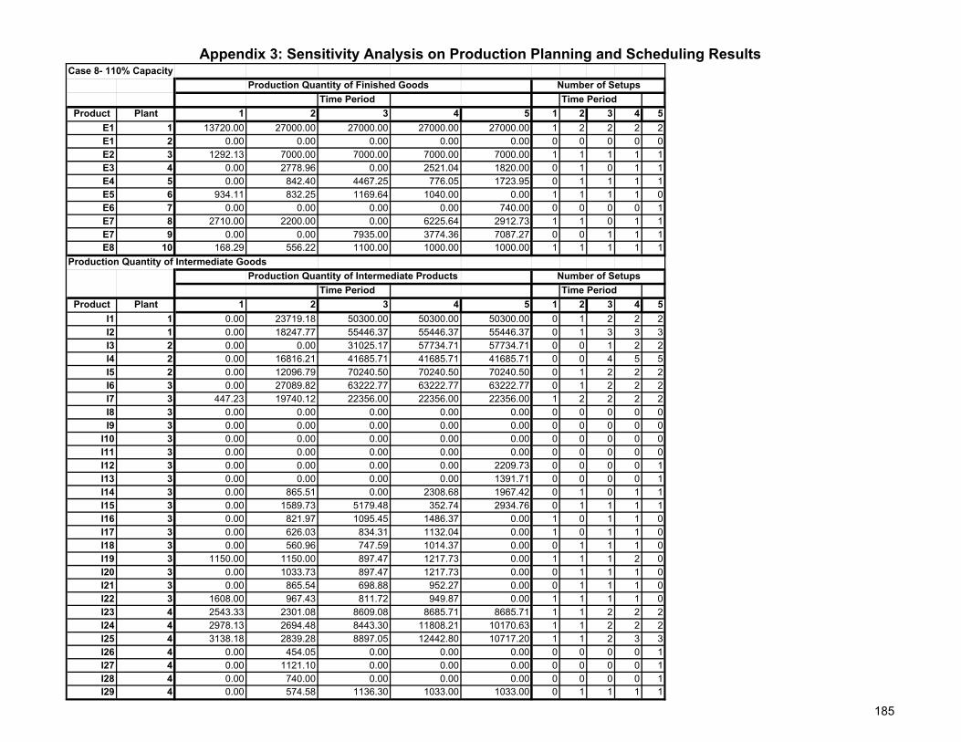
Appendix 3: Sensitivity Analysis on Production Planning and Scheduling ResultsCase 8- 110% Capacity
Production Quantity of Finished GoodsTime Period Time Period
Product Plant 1 2 3 4 5 1 2 3 4 5E1 1 13720.00 27000.00 27000.00 27000.00 27000.00 1 2 2 2 2E1 2 0.00 0.00 0.00 0.00 0.00 0 0 0 0 0E2 3 1292.13 7000.00 7000.00 7000.00 7000.00 1 1 1 1 1E3 4 0.00 2778.96 0.00 2521.04 1820.00 0 1 0 1 1E4 5 0.00 842.40 4467.25 776.05 1723.95 0 1 1 1 1E5 6 934.11 832.25 1169.64 1040.00 0.00 1 1 1 1 0E6 7 0.00 0.00 0.00 0.00 740.00 0 0 0 0 1E7 8 2710.00 2200.00 0.00 6225.64 2912.73 1 1 0 1 1E7 9 0.00 0.00 7935.00 3774.36 7087.27 0 0 1 1 1E8 10 168.29 556.22 1100.00 1000.00 1000.00 1 1 1 1 1
Production Quantity of Intermediate GoodsProduction Quantity of Intermediate Products
Time Period Time PeriodProduct Plant 1 2 3 4 5 1 2 3 4 5
I1 1 0.00 23719.18 50300.00 50300.00 50300.00 0 1 2 2 2I2 1 0.00 18247.77 55446.37 55446.37 55446.37 0 1 3 3 3I3 2 0.00 0.00 31025.17 57734.71 57734.71 0 0 1 2 2I4 2 0.00 16816.21 41685.71 41685.71 41685.71 0 0 4 5 5I5 2 0.00 12096.79 70240.50 70240.50 70240.50 0 1 2 2 2I6 3 0.00 27089.82 63222.77 63222.77 63222.77 0 1 2 2 2I7 3 447.23 19740.12 22356.00 22356.00 22356.00 1 2 2 2 2I8 3 0.00 0.00 0.00 0.00 0.00 0 0 0 0 0I9 3 0.00 0.00 0.00 0.00 0.00 0 0 0 0 0
I10 3 0.00 0.00 0.00 0.00 0.00 0 0 0 0 0I11 3 0.00 0.00 0.00 0.00 0.00 0 0 0 0 0I12 3 0.00 0.00 0.00 0.00 2209.73 0 0 0 0 1I13 3 0.00 0.00 0.00 0.00 1391.71 0 0 0 0 1I14 3 0.00 865.51 0.00 2308.68 1967.42 0 1 0 1 1I15 3 0.00 1589.73 5179.48 352.74 2934.76 0 1 1 1 1I16 3 0.00 821.97 1095.45 1486.37 0.00 1 0 1 1 0I17 3 0.00 626.03 834.31 1132.04 0.00 1 0 1 1 0I18 3 0.00 560.96 747.59 1014.37 0.00 0 1 1 1 0I19 3 1150.00 1150.00 897.47 1217.73 0.00 1 1 1 2 0I20 3 0.00 1033.73 897.47 1217.73 0.00 0 1 1 1 0I21 3 0.00 865.54 698.88 952.27 0.00 0 1 1 1 0I22 3 1608.00 967.43 811.72 949.87 0.00 1 1 1 1 0I23 4 2543.33 2301.08 8609.08 8685.71 8685.71 1 1 2 2 2I24 4 2978.13 2694.48 8443.30 11808.21 10170.63 1 1 2 2 2I25 4 3138.18 2839.28 8897.05 12442.80 10717.20 1 1 2 3 3I26 4 0.00 454.05 0.00 0.00 0.00 0 0 0 0 1I27 4 0.00 1121.10 0.00 0.00 0.00 0 0 0 0 1I28 4 0.00 740.00 0.00 0.00 0.00 0 0 0 0 1I29 4 0.00 574.58 1136.30 1033.00 1033.00 0 1 1 1 1
Number of Setups
Number of Setups
185

Appendix 3: Sensitivity Analysis on Production Planning and Scheduling ResultsCase 9- 120% Capacity
Production Quantity of Finished GoodsTime Period Time Period
Product Plant 1 2 3 4 5 1 2 3 4 5E1 1 13720.00 27000.00 27000.00 27000.00 27000.00 1 2 2 2 2E1 2 0.00 0.00 0.00 0.00 0.00 0 0 0 0 0E2 3 1292.13 7000.00 7000.00 7000.00 7000.00 1 1 1 1 1E3 4 0.00 2650.00 0.00 2650.00 1820.00 0 1 0 1 1E4 5 0.00 723.65 4586.00 1112.81 1387.19 0 1 1 1 1E5 6 181.13 1306.80 1448.07 1040.00 0.00 1 1 1 1 0E6 7 0.00 0.00 0.00 0.00 740.00 0 0 0 0 1E7 8 2710.00 2200.00 0.00 6810.26 2024.42 1 1 0 1 1E7 9 0.00 0.00 7935.00 3189.74 7975.58 0 0 1 1 1E8 10 168.29 1063.96 1100.00 1000.00 1000.00 1 1 1 1 1
Production Quantity of Intermediate GoodsProduction Quantity of Intermediate Products
Time Period Time PeriodProduct Plant 1 2 3 4 5 1 2 3 4 5
I1 1 0.00 17262.39 52452.26 52452.26 52452.26 0 1 2 2 2I2 1 0.00 18247.77 55446.37 55446.37 55446.37 0 1 3 3 3I3 2 0.00 0.00 0.00 69251.17 77243.43 0 0 0 2 2I4 2 0.00 0.00 30330.50 55771.43 55771.43 0 0 3 5 5I5 2 0.00 12096.79 70240.50 70240.50 70240.50 0 1 2 2 2I6 3 0.00 27089.82 63222.77 63222.77 63222.77 0 1 2 2 2I7 3 447.23 19740.12 22356.00 22356.00 22356.00 1 2 2 2 2I8 3 0.00 0.00 0.00 0.00 0.00 0 0 0 0 0I9 3 0.00 0.00 0.00 0.00 0.00 0 0 0 0 0
I10 3 0.00 0.00 0.00 0.00 0.00 0 0 0 0 0I11 3 0.00 0.00 0.00 0.00 0.00 0 0 0 0 0I12 3 0.00 0.00 0.00 0.00 2209.73 0 0 0 0 1I13 3 0.00 0.00 0.00 0.00 1391.71 0 0 0 0 1I14 3 0.00 309.54 0.00 2864.65 1967.42 0 1 0 1 1I15 3 0.00 738.62 6030.59 1463.35 1824.15 0 1 1 1 1I16 3 0.00 0.00 1628.62 1775.17 0.00 0 0 1 1 0I17 3 0.00 0.00 1240.38 1352.00 0.00 0 0 1 1 0I18 3 0.00 0.00 1111.45 1211.47 0.00 0 0 1 1 0I19 3 1150.00 476.58 1334.28 1454.34 0.00 1 1 2 2 0I20 3 0.00 360.31 1334.28 1454.34 0.00 0 1 1 1 0I21 3 0.00 497.78 881.61 1137.30 0.00 0 1 1 1 0I22 3 197.58 1425.46 1579.55 1134.43 0.00 1 1 1 1 0I23 4 2543.33 2064.69 7446.97 9384.96 9384.96 1 1 2 2 2I24 4 2978.13 2417.67 8720.10 10989.42 10989.42 1 1 2 2 2I25 4 3138.18 2547.60 9188.73 11580.00 11580.00 1 1 2 3 3I26 4 0.00 0.00 0.00 0.00 454.05 0 0 0 0 1I27 4 0.00 0.00 0.00 0.00 1121.10 0 0 0 0 1I28 4 0.00 0.00 0.00 0.00 740.00 0 0 0 0 1I29 4 0.00 1099.07 1136.30 1033.00 1033.00 0 1 1 1 1
Number of Setups
Number of Setups
186

Appendix 3: Sensitivity Analysis on Production Planning and Scheduling ResultsCase 10- 80% Initial Inventory
Production Quantity of Finished GoodsTime Period Time Period
Product Plant 1 2 3 4 5 1 2 3 4 5E1 1 16376.00 27000.00 27000.00 27000.00 27000.00 2 2 2 2 2E1 2 0.00 0.00 0.00 0.00 0.00 0 0 0 0 0E2 3 2433.70 7000.00 7000.00 7000.00 7000.00 1 1 1 1 1E3 4 868.84 1781.16 0.00 2650.00 1820.00 1 1 0 1 1E4 5 0.00 1666.45 4594.16 0.00 2321.31 0 1 1 0 1E5 6 1339.69 816.00 780.31 1040.00 0.00 1 1 1 1 0E6 7 0.00 0.00 0.00 0.00 842.00 0 0 0 0 1E7 8 0.00 0.00 0.00 1785.58 4042.13 0 0 0 1 1E7 9 2710.00 2200.00 7949.42 8200.00 5957.87 1 1 1 1 1E8 10 134.63 764.98 1100.00 1000.00 1000.00 1 1 1 1 1
Production Quantity of Intermediate GoodsProduction Quantity of Intermediate Products
Time Period Time PeriodProduct Plant 1 2 3 4 5 1 2 3 4 5
I1 1 0.00 34790.82 52452.26 52452.26 52452.26 0 2 2 2 2I2 1 0.00 36776.76 55446.37 55446.37 55446.37 0 2 3 3 3I3 2 0.00 11829.87 64501.43 64501.43 64501.43 0 1 2 2 2I4 2 0.00 37422.29 46571.43 46571.43 46571.43 0 4 4 4 4I5 2 0.00 37773.63 70240.50 70240.50 70240.50 0 1 2 2 2I6 3 0.00 46960.96 63222.77 63222.77 63222.77 0 2 2 2 2I7 3 2736.28 22356.00 22356.00 22356.00 22356.00 1 2 2 2 2I8 3 0.00 0.00 0.00 0.00 0.00 0 0 0 0 0I9 3 0.00 0.00 0.00 0.00 0.00 0 0 0 0 0
I10 3 0.00 0.00 0.00 0.00 0.00 0 0 0 0 0I11 3 0.00 0.00 0.00 0.00 0.00 0 0 0 0 0I12 3 0.00 0.00 1015.67 1100.93 2976.31 0 0 1 1 1I13 3 0.00 0.00 0.00 621.51 2260.57 0 0 0 1 1I14 3 0.00 820.56 0.00 2864.65 1967.42 0 1 0 1 1I15 3 0.00 2020.99 6041.32 0.00 3052.53 0 1 1 0 1I16 3 0.00 1101.99 1578.21 1400.16 0.00 0 1 1 1 0I17 3 0.00 839.29 1201.99 1066.38 0.00 0 1 1 1 0I18 3 0.00 752.05 1077.05 955.54 0.00 0 1 1 1 0I19 3 957.54 1246.55 989.79 1450.29 0.00 1 2 1 2 0I20 3 0.00 1191.08 1292.97 1147.11 0.00 0 1 1 1 0I21 3 0.00 974.80 774.01 1134.13 0.00 0 1 1 1 0I22 3 1461.34 890.09 851.16 1134.43 0.00 1 1 1 1 0I23 4 2543.33 2064.69 7460.51 9371.43 9384.96 1 1 2 2 2I24 4 2978.13 2417.67 8735.96 10973.57 10989.42 1 1 2 2 2I25 4 3138.18 2547.60 9205.43 11563.30 11580.00 1 1 2 3 3I26 4 0.00 0.00 516.63 0.00 0.00 0 0 1 0 0I27 4 0.00 0.00 1275.63 0.00 0.00 0 0 1 0 0I28 4 0.00 0.00 842.00 0.00 0.00 0 0 1 1 0I29 4 0.00 790.22 1136.30 1033.00 1033.00 0 1 1 1 1
Number of Setups
Number of Setups
187

Appendix 3: Sensitivity Analysis on Production Planning and Scheduling ResultsCase 11- 90% Initial Inventory
Production Quantity of Finished GoodsTime Period Time Period
Product Plant 1 2 3 4 5 1 2 3 4 5E1 1 15048.00 27000.00 27000.00 27000.00 27000.00 1 2 2 2 2E1 2 0.00 0.00 0.00 0.00 0.00 0 0 0 0 0E2 3 1862.92 7000.00 7000.00 7000.00 7000.00 1 1 1 1 1E3 4 697.20 1952.80 0.00 2650.00 1820.00 1 1 0 1 1E4 5 0.00 1202.46 4577.76 0.00 2415.57 0 2 1 0 1E5 6 1474.15 674.14 787.71 1040.00 0.00 1 1 1 1 0E6 7 0.00 0.00 0.00 0.00 791.00 0 0 0 0 1E7 8 2710.00 2200.00 0.00 5641.03 3907.16 1 1 0 1 1E7 9 0.00 0.00 8200.00 4108.40 6078.42 0 0 1 1 1E8 10 151.46 660.60 1100.00 1000.00 1000.00 1 1 1 1 1
Production Quantity of Intermediate GoodsProduction Quantity of Intermediate Products
Time Period Time PeriodProduct Plant 1 2 3 4 5 1 2 3 4 5
I1 1 0.00 26026.61 52452.26 52452.26 52452.26 0 1 2 2 2I2 1 0.00 27512.27 55446.37 55446.37 55446.37 0 2 3 3 3I3 2 0.00 0.00 46911.52 64501.43 64501.43 0 0 1 2 2I4 2 0.00 19790.68 46571.43 46571.43 46571.43 0 2 4 4 4I5 2 0.00 24935.21 70240.50 70240.50 70240.50 0 1 2 2 2I6 3 0.00 37025.39 63222.77 63222.77 63222.77 0 1 2 2 2I7 3 451.26 22188.55 22356.00 22356.00 22356.00 1 2 2 2 2I8 3 0.00 0.00 0.00 0.00 0.00 0 0 0 0 0I9 3 0.00 0.00 0.00 0.00 0.00 0 0 0 0 0
I10 3 0.00 0.00 0.00 0.00 0.00 0 0 0 0 0I11 3 0.00 0.00 0.00 0.00 0.00 0 0 0 0 0I12 3 0.00 0.00 0.00 659.59 2991.73 0 0 0 1 1I13 3 0.00 0.00 0.00 0.00 2136.89 0 0 0 0 1I14 3 0.00 565.05 0.00 2864.65 1967.42 1 1 0 1 1I15 3 0.00 1389.55 6019.75 0.00 3176.47 0 1 1 0 1I16 3 0.00 761.81 1394.90 1585.36 0.00 0 1 1 1 0I17 3 0.00 580.21 1062.38 1207.43 0.00 0 1 1 1 0I18 3 0.00 519.90 951.95 1081.93 0.00 0 1 1 1 0I19 3 1077.24 1010.82 991.34 1450.29 0.00 1 1 1 2 0I20 3 0.00 948.41 1142.80 1298.83 0.00 0 1 1 1 0I21 3 0.00 790.46 775.23 1134.13 0.00 0 1 1 1 0I22 3 1608.00 735.35 859.23 1134.43 0.00 1 1 1 1 0I23 4 2543.33 2064.69 8502.34 8343.13 9371.43 1 1 2 2 2I24 4 2978.13 2417.67 9011.32 10714.05 10973.57 1 1 2 2 2I25 4 3138.18 2547.60 9495.60 11289.83 11563.30 1 1 2 3 3I26 4 0.00 0.00 0.00 485.34 0.00 0 0 0 1 0I27 4 0.00 0.00 0.00 1198.37 0.00 0 0 0 1 0I28 4 0.00 0.00 0.00 791.00 0.00 0 0 0 1 1I29 4 0.00 682.40 1136.30 1033.00 1033.00 0 1 1 1 1
Number of Setups
Number of Setups
188

Appendix 3: Sensitivity Analysis on Production Planning and Scheduling ResultsCase 12- 110% Initial Inventory
Production Quantity of Finished GoodsTime Period Time Period
Product Plant 1 2 3 4 5 1 2 3 4 5E1 1 12392.00 27000.00 27000.00 27000.00 27000.00 1 2 2 2 2E1 2 0.00 0.00 0.00 0.00 0.00 0 0 0 0 0E2 3 721.34 7000.00 7000.00 7000.00 7000.00 1 1 1 1 1E3 4 275.92 3093.60 0.00 1930.48 1820.00 1 1 0 1 1E4 5 0.00 1986.12 2937.40 1089.38 1410.62 0 1 1 1 1E5 6 1474.15 0.00 1528.26 973.59 0.00 1 0 1 1 0E6 7 0.00 0.00 0.00 0.00 689.00 0 0 0 1 1E7 8 2710.00 2200.00 0.00 1801.37 3666.07 1 1 0 1 1E7 9 0.00 0.00 8200.00 7948.05 6319.51 0 0 1 1 1E8 10 185.12 451.85 1100.00 1000.00 1000.00 1 1 1 1 1
Production Quantity of Intermediate GoodsProduction Quantity of Intermediate Products
Time Period Time PeriodProduct Plant 1 2 3 4 5 1 2 3 4 5
I1 1 0.00 8498.18 52452.26 52452.26 52452.26 0 1 2 2 2I2 1 0.00 8983.28 55446.37 55446.37 55446.37 0 1 3 3 3I3 2 0.00 0.00 0.00 52573.39 64501.43 0 0 0 2 2I4 2 0.00 0.00 31098.89 46571.43 46571.43 0 0 3 4 4I5 2 0.00 0.00 69498.86 70240.50 70240.50 0 0 2 2 2I6 3 0.00 17154.25 63222.77 63222.77 63222.77 0 1 2 2 2I7 3 447.23 17287.65 22356.00 22356.00 22356.00 1 2 2 2 2I8 3 0.00 0.00 0.00 0.00 0.00 0 0 0 0 0I9 3 0.00 0.00 0.00 0.00 0.00 0 0 0 0 0
I10 3 0.00 0.00 0.00 0.00 0.00 0 0 0 0 0I11 3 0.00 0.00 0.00 0.00 0.00 0 0 0 0 0I12 3 0.00 0.00 0.00 0.00 768.14 0 0 0 0 1I13 3 0.00 0.00 0.00 0.00 646.53 0 0 0 0 1I14 3 0.00 831.83 0.00 2086.85 1967.42 0 1 0 1 1I15 3 0.00 2377.47 3862.68 1432.54 1854.96 0 1 1 1 1I16 3 0.00 0.00 1403.69 1661.82 0.00 0 1 1 1 0I17 3 0.00 0.00 1069.07 1265.66 0.00 0 0 1 1 0I18 3 0.00 0.00 957.95 1134.11 0.00 0 1 1 1 0I19 3 1150.00 639.24 1150.00 1361.47 0.00 1 1 1 2 0I20 3 0.00 396.34 1150.00 1361.47 0.00 0 1 1 1 0I21 3 0.00 560.74 889.72 883.09 0.00 0 1 1 1 0I22 3 1608.00 0.00 1667.03 1061.99 0.00 1 0 1 1 0I23 4 2543.33 2064.69 8369.74 8475.73 9371.43 1 1 2 2 2I24 4 2978.13 2417.67 9011.32 10714.05 10973.57 1 1 2 2 2I25 4 3138.18 2547.60 9495.60 11289.83 11563.30 1 1 2 3 3I26 4 0.00 0.00 0.00 422.75 0.00 0 0 0 1 1I27 4 0.00 0.00 0.00 1043.84 0.00 0 0 0 1 1I28 4 0.00 0.00 0.00 689.00 0.00 0 0 0 1 1I29 4 0.00 466.76 1136.30 1033.00 1033.00 0 1 1 1 1
Number of Setups
Number of Setups
189

Appendix 3: Sensitivity Analysis on Production Planning and Scheduling ResultsCase 13- 120% Initial Inventory
Production Quantity of Finished GoodsTime Period Time Period
Product Plant 1 2 3 4 5 1 2 3 4 5E1 1 11064.00 27000.00 27000.00 27000.00 27000.00 1 2 2 2 2E1 2 0.00 0.00 0.00 0.00 0.00 0 0 0 0 0E2 3 150.56 7000.00 7000.00 7000.00 7000.00 1 1 1 1 1E3 4 228.24 2608.14 0.00 2463.62 1820.00 1 1 0 1 1E4 5 0.00 2727.35 2957.85 254.89 1097.28 0 1 1 1 1E5 6 1474.15 0.00 1519.03 982.82 0.00 1 0 1 1 0E6 7 0.00 0.00 0.00 0.00 638.00 0 0 0 1 1E7 8 2710.00 2200.00 0.00 1801.37 3545.52 1 1 0 1 1E7 9 0.00 0.00 8200.00 7948.05 6440.05 0 0 1 1 1E8 10 201.94 347.47 1100.00 1000.00 1000.00 1 1 1 1 1
Production Quantity of Intermediate GoodsProduction Quantity of Intermediate Products
Time Period Time PeriodProduct Plant 1 2 3 4 5 1 2 3 4 5
I1 1 0.00 0.00 52186.23 52452.26 52452.26 0 0 2 2 2I2 1 0.00 0.00 55165.15 55446.37 55446.37 0 0 3 3 3I3 2 0.00 0.00 0.00 23153.62 64501.43 0 0 0 1 2I4 2 0.00 0.00 13467.28 46571.43 46571.43 0 0 2 4 4I5 2 0.00 0.00 56660.44 70240.50 70240.50 0 0 2 2 2I6 3 0.00 7218.68 63222.77 63222.77 63222.77 0 1 2 2 2I7 3 431.37 14851.05 22356.00 22356.00 22356.00 1 1 2 2 2I8 3 0.00 0.00 0.00 0.00 0.00 0 0 0 0 0I9 3 0.00 0.00 0.00 0.00 0.00 0 0 0 0 0
I10 3 0.00 0.00 0.00 0.00 0.00 0 0 0 0 0I11 3 0.00 0.00 0.00 0.00 0.00 0 0 0 0 0I12 3 0.00 0.00 0.00 0.00 0.00 0 0 0 0 0I13 3 0.00 0.00 0.00 0.00 0.00 0 0 0 0 0I14 3 0.00 0.00 0.00 2663.17 1967.42 0 0 0 1 1I15 3 0.00 3330.89 3889.57 335.19 1442.93 0 1 1 1 1I16 3 0.00 0.00 1049.65 1677.58 0.00 0 0 1 1 0I17 3 0.00 0.00 799.43 1277.67 0.00 0 0 1 1 0I18 3 0.00 0.00 716.33 1144.86 0.00 0 0 1 1 0I19 3 1436.32 230.94 1144.58 1374.38 0.00 2 1 1 2 0I20 3 0.00 147.74 1144.58 1374.38 0.00 0 1 1 1 0I21 3 0.00 180.60 895.06 1074.77 0.00 0 1 1 1 0I22 3 1608.00 0.00 1656.96 1072.06 0.00 1 0 1 1 0I23 4 2543.33 2064.69 8303.44 8542.03 9371.43 1 1 2 2 2I24 4 2978.13 2417.67 9011.32 10714.05 10973.57 1 1 2 2 2I25 4 3138.18 2547.60 9495.60 11289.83 11563.30 1 1 2 3 3I26 4 0.00 0.00 0.00 391.46 0.00 0 0 0 1 1I27 4 0.00 0.00 0.00 966.57 0.00 0 0 0 1 1I28 4 0.00 0.00 0.00 638.00 0.00 0 0 0 1 1I29 4 0.00 358.93 1136.30 1033.00 1033.00 0 1 1 1 1
Number of Setups
Number of Setups
190

Appendix 3: Sensitivity Analysis on Production Planning and Scheduling ResultsCase 14- Setup to Inventory Cost Ratio- 25
Production Quantity of Finished GoodsTime Period Time Period
Product Plant 1 2 3 4 5 1 2 3 4 5E1 1 11064.00 27000.00 27000.00 27000.00 27000.00 1 2 2 2 2E1 2 0.00 0.00 0.00 0.00 0.00 0 0 0 0 0E2 3 150.56 7000.00 7000.00 7000.00 7000.00 1 1 1 1 1E3 4 2650.00 0.00 0.00 2650.00 1820.00 1 0 0 1 1E4 5 0.00 1362.34 4577.76 0.00 1097.28 0 1 1 0 1E5 6 0.00 2148.29 787.71 1040.00 0.00 0 1 1 1 0E6 7 0.00 0.00 0.00 0.00 638.00 0 0 0 0 1E7 8 2710.00 2200.00 0.00 5641.03 3559.95 1 1 0 1 1E7 9 0.00 0.00 8200.00 4093.97 6440.05 0 0 1 1 1E8 10 0.00 549.41 1100.00 1000.00 1000.00 0 1 1 1 1
Production Quantity of Intermediate GoodsProduction Quantity of Intermediate Products
Time Period Time PeriodProduct Plant 1 2 3 4 5 1 2 3 4 5
I1 1 0.00 0.00 52186.23 52452.26 52452.26 0 0 2 2 2I2 1 0.00 0.00 55165.15 55446.37 55446.37 0 0 3 3 3I3 2 0.00 0.00 0.00 23659.73 63995.31 0 0 0 1 2I4 2 0.00 0.00 23054.14 37350.00 46206.00 0 0 2 3 4I5 2 0.00 0.00 95141.43 51000.00 51000.00 0 0 2 1 1I6 3 0.00 7218.68 63222.77 63222.77 63222.77 0 1 2 2 2I7 3 510.93 14771.49 22356.00 22356.00 22356.00 1 1 2 2 2I8 3 0.00 0.00 0.00 0.00 0.00 0 0 0 0 0I9 3 0.00 0.00 0.00 0.00 0.00 0 0 0 0 0
I10 3 0.00 0.00 0.00 0.00 0.00 0 0 0 0 0I11 3 0.00 0.00 0.00 0.00 0.00 0 0 0 0 0I12 3 0.00 0.00 0.00 0.00 0.00 0 0 0 0 0I13 3 0.00 0.00 0.00 0.00 0.00 0 0 0 0 0I14 3 0.00 0.00 0.00 2663.17 1967.42 0 0 0 1 1I15 3 1535.90 0.00 6019.75 0.00 1442.93 1 0 1 0 1I16 3 0.00 0.00 2727.23 0.00 0.00 0 0 1 0 0I17 3 0.00 0.00 2077.10 0.00 0.00 0 0 1 0 0I18 3 0.00 0.00 1861.20 0.00 0.00 0 0 1 0 0I19 3 0.00 1744.60 991.34 1450.29 0.00 0 2 1 2 0I20 3 0.00 225.07 2441.63 0.00 0.00 0 1 1 0 0I21 3 0.00 241.07 775.23 1134.13 0.00 0 1 1 1 0I22 3 0.00 2343.35 859.23 1134.43 0.00 0 2 1 1 0I23 4 2543.33 2064.69 8289.91 8542.03 9384.96 1 1 2 2 2I24 4 2978.13 2417.67 9011.32 10698.20 10989.42 1 1 2 2 2I25 4 3138.18 2547.60 9495.60 11273.13 11580.00 1 1 2 3 3I26 4 0.00 0.00 0.00 391.46 0.00 0 0 0 1 1I27 4 0.00 0.00 0.00 966.57 0.00 0 0 0 1 1I28 4 0.00 0.00 0.00 638.00 0.00 0 0 0 1 0I29 4 0.00 358.93 1136.30 1033.00 1033.00 0 1 1 1 1
Number of Setups
Number of Setups
191
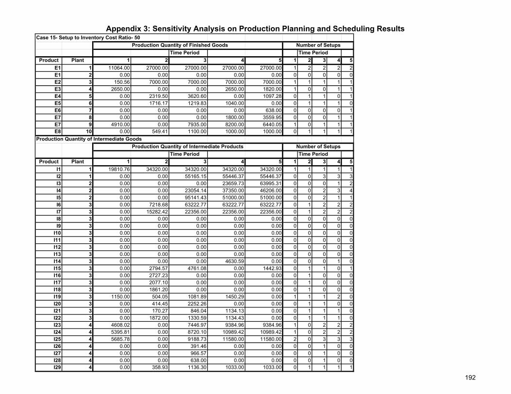
Appendix 3: Sensitivity Analysis on Production Planning and Scheduling ResultsCase 15- Setup to Inventory Cost Ratio- 50
Production Quantity of Finished GoodsTime Period Time Period
Product Plant 1 2 3 4 5 1 2 3 4 5E1 1 11064.00 27000.00 27000.00 27000.00 27000.00 1 2 2 2 2E1 2 0.00 0.00 0.00 0.00 0.00 0 0 0 0 0E2 3 150.56 7000.00 7000.00 7000.00 7000.00 1 1 1 1 1E3 4 2650.00 0.00 0.00 2650.00 1820.00 1 0 0 1 1E4 5 0.00 2319.50 3620.60 0.00 1097.28 0 1 1 0 1E5 6 0.00 1716.17 1219.83 1040.00 0.00 0 1 1 1 0E6 7 0.00 0.00 0.00 0.00 638.00 0 0 0 0 1E7 8 0.00 0.00 0.00 1800.00 3559.95 0 0 0 1 1E7 9 4910.00 0.00 7935.00 8200.00 6440.05 1 0 1 1 1E8 10 0.00 549.41 1100.00 1000.00 1000.00 0 1 1 1 1
Production Quantity of Intermediate GoodsProduction Quantity of Intermediate Products
Time Period Time PeriodProduct Plant 1 2 3 4 5 1 2 3 4 5
I1 1 19810.76 34320.00 34320.00 34320.00 34320.00 1 1 1 1 1I2 1 0.00 0.00 55165.15 55446.37 55446.37 0 0 3 3 3I3 2 0.00 0.00 0.00 23659.73 63995.31 0 0 0 1 2I4 2 0.00 0.00 23054.14 37350.00 46206.00 0 0 2 3 4I5 2 0.00 0.00 95141.43 51000.00 51000.00 0 0 2 1 1I6 3 0.00 7218.68 63222.77 63222.77 63222.77 0 1 2 2 2I7 3 0.00 15282.42 22356.00 22356.00 22356.00 0 1 2 2 2I8 3 0.00 0.00 0.00 0.00 0.00 0 0 0 0 0I9 3 0.00 0.00 0.00 0.00 0.00 0 0 0 0 0
I10 3 0.00 0.00 0.00 0.00 0.00 0 0 0 0 0I11 3 0.00 0.00 0.00 0.00 0.00 0 0 0 0 0I12 3 0.00 0.00 0.00 0.00 0.00 0 0 0 0 0I13 3 0.00 0.00 0.00 0.00 0.00 0 0 0 0 0I14 3 0.00 0.00 0.00 4630.59 0.00 0 0 0 1 0I15 3 0.00 2794.57 4761.08 0.00 1442.93 0 1 1 0 1I16 3 0.00 2727.23 0.00 0.00 0.00 0 1 0 0 0I17 3 0.00 2077.10 0.00 0.00 0.00 0 1 0 0 0I18 3 0.00 1861.20 0.00 0.00 0.00 0 1 0 0 0I19 3 1150.00 504.05 1081.89 1450.29 0.00 1 1 1 2 0I20 3 0.00 414.45 2252.26 0.00 0.00 0 1 1 0 0I21 3 0.00 170.27 846.04 1134.13 0.00 0 1 1 1 0I22 3 0.00 1872.00 1330.59 1134.43 0.00 0 1 1 1 0I23 4 4608.02 0.00 7446.97 9384.96 9384.96 1 0 2 2 2I24 4 5395.81 0.00 8720.10 10989.42 10989.42 1 0 2 2 2I25 4 5685.78 0.00 9188.73 11580.00 11580.00 2 0 3 3 3I26 4 0.00 0.00 391.46 0.00 0.00 0 0 1 0 0I27 4 0.00 0.00 966.57 0.00 0.00 0 0 1 0 0I28 4 0.00 0.00 638.00 0.00 0.00 0 0 1 0 0I29 4 0.00 358.93 1136.30 1033.00 1033.00 0 1 1 1 1
Number of Setups
Number of Setups
192

Appendix 3: Sensitivity Analysis on Production Planning and Scheduling ResultsCase 16- Setup to Inventory Cost Ratio- 0.1
Production Quantity of Finished GoodsTime Period Time Period
Product Plant 1 2 3 4 5 1 2 3 4 5E1 1 11064.00 27000.00 27000.00 27000.00 27000.00 1 2 2 2 2E1 2 0.00 0.00 0.00 0.00 0.00 0 0 0 0 0E2 3 150.56 7000.00 7000.00 7000.00 7000.00 1 1 1 1 1E3 4 566.27 2909.21 0.00 1824.52 1820.00 1 1 0 1 1E4 5 0.00 876.21 3661.17 1402.72 1097.28 0 1 1 1 1E5 6 1474.15 395.17 1201.51 905.17 0.00 1 1 1 1 0E6 7 0.00 0.00 0.00 0.00 638.00 0 0 0 0 1E7 8 2710.00 2200.00 0.00 5641.03 3545.52 1 1 0 1 1E7 9 0.00 0.00 7963.85 4344.55 6440.05 0 0 1 1 1E8 10 201.94 347.47 1100.00 1000.00 1000.00 1 1 1 1 1
Production Quantity of Intermediate GoodsProduction Quantity of Intermediate Products
Time Period Time PeriodProduct Plant 1 2 3 4 5 1 2 3 4 5
I1 1 0.00 0.00 52186.23 52452.26 52452.26 0 0 2 2 2I2 1 0.00 0.00 55165.15 55446.37 55446.37 0 0 3 3 3I3 2 0.00 0.00 0.00 23153.62 64501.43 0 0 0 1 2I4 2 0.00 0.00 13467.28 46571.43 46571.43 0 0 2 4 4I5 2 0.00 0.00 56660.44 70240.50 70240.50 0 0 2 2 2I6 3 0.00 7218.68 63222.77 63222.77 63222.77 0 1 2 2 2I7 3 431.37 14851.05 22356.00 22356.00 22356.00 1 1 2 2 2I8 3 0.00 0.00 0.00 0.00 0.00 0 0 0 0 0I9 3 0.00 0.00 0.00 0.00 0.00 0 0 0 0 0
I10 3 0.00 0.00 0.00 0.00 0.00 0 0 0 0 0I11 3 0.00 0.00 0.00 0.00 0.00 0 0 0 0 0I12 3 0.00 0.00 0.00 0.00 0.00 0 0 0 0 0I13 3 0.00 0.00 0.00 0.00 0.00 0 0 0 0 0I14 3 0.00 690.86 0.00 1972.30 1967.42 0 1 0 1 1I15 3 0.00 896.64 4814.44 1844.57 1442.93 0 1 1 1 1I16 3 0.00 0.00 1182.19 1545.04 0.00 0 0 1 1 0I17 3 0.00 0.00 900.37 1176.72 0.00 0 0 1 1 0I18 3 0.00 0.00 806.79 1054.41 0.00 0 0 1 1 0I19 3 1436.32 406.06 1078.05 1265.80 0.00 2 1 1 2 0I20 3 0.00 322.86 1078.05 1265.80 0.00 0 1 1 1 0I21 3 0.00 317.54 843.03 989.86 0.00 0 1 1 1 0I22 3 1608.00 431.05 1310.61 987.36 0.00 1 1 1 1 0I23 4 2543.33 2064.69 7474.04 9371.43 9371.43 1 1 2 2 2I24 4 2978.13 2417.67 8751.81 10973.57 10973.57 1 1 2 2 2I25 4 3138.18 2547.60 9222.13 11563.30 11563.30 1 1 2 3 3I26 4 0.00 0.00 391.46 0.00 0.00 0 0 1 0 0I27 4 0.00 0.00 966.57 0.00 0.00 0 0 1 0 0I28 4 0.00 0.00 638.00 0.00 0.00 0 0 1 1 1I29 4 0.00 358.93 1136.30 1033.00 1033.00 0 1 1 1 1
Number of Setups
Number of Setups
193

Appendix 3: Sensitivity Analysis on Production Planning and Scheduling ResultsCase 17- Setup to Inventory Cost Ratio- 0.5
Production Quantity of Finished GoodsTime Period Time Period
Product Plant 1 2 3 4 5 1 2 3 4 5E1 1 11064.00 27000.00 27000.00 27000.00 27000.00 1 2 2 2 2E1 2 0.00 0.00 0.00 0.00 0.00 0 0 0 0 0E2 3 150.56 7000.00 7000.00 7000.00 7000.00 1 1 1 1 1E3 4 566.27 3104.80 0.00 1628.93 1820.00 1 1 0 1 1E4 5 0.00 1452.88 3084.50 1402.72 1097.28 0 1 1 1 1E5 6 1474.15 0.00 1461.85 1040.00 0.00 1 1 1 1 0E6 7 0.00 0.00 0.00 0.00 638.00 0 0 0 1 1E7 8 2710.00 2200.00 0.00 1801.37 3545.52 1 1 0 1 1E7 9 0.00 0.00 8200.00 7948.05 6440.05 0 0 1 1 1E8 10 201.94 347.47 1100.00 1000.00 1000.00 1 1 1 1 1
Production Quantity of Intermediate GoodsProduction Quantity of Intermediate Products
Time Period Time PeriodProduct Plant 1 2 3 4 5 1 2 3 4 5
I1 1 0.00 0.00 52186.23 52452.26 52452.26 0 0 2 2 2I2 1 0.00 0.00 55165.15 55446.37 55446.37 0 0 3 3 3I3 2 0.00 0.00 0.00 23153.62 64501.43 0 0 0 1 2I4 2 0.00 0.00 13467.28 46571.43 46571.43 0 0 2 4 4I5 2 0.00 0.00 56660.44 70240.50 70240.50 0 0 2 2 2I6 3 0.00 7218.68 63222.77 63222.77 63222.77 0 1 2 2 2I7 3 431.37 14851.05 22356.00 22356.00 22356.00 1 1 2 2 2I8 3 0.00 0.00 0.00 0.00 0.00 0 0 0 0 0I9 3 0.00 0.00 0.00 0.00 0.00 0 0 0 0 0
I10 3 0.00 0.00 0.00 0.00 0.00 0 0 0 0 0I11 3 0.00 0.00 0.00 0.00 0.00 0 0 0 0 0I12 3 0.00 0.00 0.00 0.00 0.00 0 0 0 0 0I13 3 0.00 0.00 0.00 0.00 0.00 0 0 0 0 0I14 3 0.00 902.30 0.00 1760.87 1967.42 0 1 0 1 1I15 3 0.00 1654.96 4056.12 1844.57 1442.93 0 1 1 1 1I16 3 0.00 0.00 1182.19 1545.04 0.00 0 0 1 1 0I17 3 0.00 0.00 900.37 1176.72 0.00 0 0 1 1 0I18 3 0.00 0.00 806.79 1054.41 0.00 0 0 1 1 0I19 3 1436.32 351.51 1132.60 1265.80 0.00 2 1 1 2 0I20 3 0.00 268.30 1132.60 1265.80 0.00 0 1 1 1 0I21 3 0.00 274.88 885.69 989.86 0.00 0 1 1 1 0I22 3 1608.00 0.00 1594.59 1134.43 0.00 1 0 1 1 0I23 4 2543.33 2064.69 8303.44 8542.03 9371.43 1 1 2 2 2I24 4 2978.13 2417.67 9011.32 10714.05 10973.57 1 1 2 2 2I25 4 3138.18 2547.60 9495.60 11289.83 11563.30 1 1 2 3 3I26 4 0.00 0.00 0.00 391.46 0.00 0 0 0 1 1I27 4 0.00 0.00 0.00 966.57 0.00 0 0 0 1 1I28 4 0.00 0.00 0.00 638.00 0.00 0 0 0 1 1I29 4 0.00 358.93 1136.30 1033.00 1033.00 0 1 1 1 1
Number of Setups
Number of Setups
194