Production methodologies applied to the fluid system ...

Production methodologies applied to the fluid system

outfitting on a construction and repair shipyard

Joao Jose Ludovice Paixao de Melo

Thesis to obtain the Master of Science Degree in

Naval Architecture and Marine Engineering

Supervisors: Engenheiro Francisco Jorge Gomes Lopes

Professor Doutor Carlos Pancadas Guedes Soares

Examination Committee

Chairperson:

Supervisor: Engenheiro Francisco Jorge Gomes Lopes

Members of the Committee:

October 2018

iii

Acknowledgments

Em primeiro lugar, quero expressar a minha gratidão ao meu orientador de tese, Professor Gomes

Lopes, pelo apoio prestado na elaboração deste trabalho. A sua permanente disponibilidade, a

orientação segura, as críticas construtivas e as sugestões valiosas permitiram torná-lo um

verdadeiro processo de desenvolvimento pessoal e profissional. Gostaria também de agradecer ao

Professor Doutor Carlos Guedes Soares e ao Professor Gomes Lopes, porque a pesquisa em que

se baseou grande parte desta tese só foi possível graças à oportunidade que me deram de realizar

a dissertação de mestrado no estaleiro da Atlantic Eagle Shipbuilding. Quero fazer um

agradecimento especial ao Eng. Bruno Costa, ao Engenheiro Raul Leite e a toda a equipa da Atlantic

Eagle Shipbuilding, por toda a disponibilidade para a recolha presencial de dados, no estaleiro, e

por todos os documentos técnico fornecidos para a realização desta dissertação. Por fim, quero

agradecer à minha família, em particular à minha mãe, pelo apoio incondicional que me garantiram

em todos os momentos deste trabalho.

v

Abstract

Due to the competitiveness of shipbuilding environment, shipyards try to optimize production efficiencies

in terms of time, costs and quality and obtaining better results.

Modular Outfitting (MO) is an approach that consists in the installation of outfit systems on a structural

block prior to shipboard erection. Traditional Outfitting (TO) consist in on-board outfitting installation on

a building berth before launching or on-board after launching and as it allows parallel assembly of various

outfitting systems, it has the potential to reduce the assembling workload.

The dissertation scope is to compare the workload (expressed in man-hours - Mh) of a ferry vessel

bilge’s fluid system (Haksolok built in Atlantic Eagle Shipyard) assembly performed by TO versus MO.

Three questions are addressed regarding MO implementation versus TO in three selected bilge piping

zones of higher complexity concerning: workload differences; layout changes and risk management

The workload, measured in man-hours, used in the assembling procedure by MO, represented a

reduction of 549 Man-hours or a gain of 74% versus TO.

There are advantages in the new layout concerning distance between work stations, space for outfitting

activities and outfitting work flow hub creation.

A risk assessment was performed, and the most critical risks were associated to: Design Process;

Dimensional Control and Running Test in Shop Process; Module Transportation and Fitting on Block

Process and On-block Assembly Fitting and Installing Process. The higher risk score regards Effective

Schedule Coordination between Block and Module Block

To control the major risks a list of nine critical success factors was defined, being the qualification of

the labor force and the update of the equipment, the most critical.

Keywords

Modular Outfitting, Integrated construction, zone outfitting, systematic layout planning, risk

management critical success factors, piping, outfitting

vii

Resumo

Devido à competitividade do ambiente da construção naval, os estaleiros navais tentam optimizar a

eficiência da produção em termos de tempo, custos e qualidade.

O aprestamento modular (MO) consiste na instalação de sistemas e equipamentos num bloco estrutural

antes da montagem do navio. O aprestamento tradicional (TO) consiste na instalação do equipamento

a bordo do navio antes do lançamento (na doca/rampa ou a bordo após o lançamento). O MO tem o

potencial de reduzir a carga de trabalho de montagem dado permitir a montagem paralela de vários

sistemas de equipamentos.

O objectivo desta dissertação é comparar a carga de trabalho da instalação, medida em horas-homem

de um sistema de esgoto de um ferry (navio Haksolok construído no estaleiro Atlantic Eagle) utilizada

pelo método TO com a utilizada pelo método MO.

O estudo centrou-se em três questões relativas à implementação de MO versus TO em três zonas

selecionadas do Sistema de Esgoto devido a maior complexidade referentes às diferenças de carga de

trabalho; às mudanças de arranjo geral do estaleiro e à gestão do risco.

Verificou-se que a carga de trabalho utilizada no procedimento de montagem por MO, representou uma

redução de 549 horas-homem ou um ganho de 74% versus TO.

Foram identificadas vantagens no novo layout no que concerne à distância entre estações de trabalho,

espaço para atividades de aprestamento e adequação da criação de pontos logísticos para

aprestamento.

Os riscos mais críticos foram os associados a: processo de design; controlo dimensional e teste de

funcionamento no processo de manufactura; transporte dos módulos, montagem nos blocos, processo

de instalação e montagem no bloco. O maior factor de risco correspondeu à coordenação do

planeamento de montagem entre módulo e bloco.

Para controlar os principais riscos foi definida uma lista de nove fatores críticos de sucesso, sendo os

mais críticos, a qualificação da força de trabalho e a atualização do equipamento. Palavras Chave

Aprestamento por construção modular, construção naval integrada, aprestamento por zonas,

systematic layout planning, gestão de risco, factores críticos de sucesso, encanamentos,

aprestamento

ix

Contents

1 Introduction .............................................................................................................................. 2

1.1 Dissertation’s scope of work ............................................................................................. 4 1.2 Portuguese shipbuilding and ship repair ........................................................................... 6

1.2.1 Portuguese Shipyards ........................................................................................... 6 1.2.2 Atlanticeagle Shipbuilding (AES) ........................................................................... 7

1.3 Haksolok ferry vessel ........................................................................................................ 8 2 Behind State of Art ................................................................................................................ 11

2.1 Preliminary concepts on ships life cycle ......................................................................... 13 2.2 Outfitting .......................................................................................................................... 15

2.2.1 Traditional Outfitting ............................................................................................ 16 2.2.2 Modular Outfitting ................................................................................................ 16 2.2.3 Modular Outfitting advantages compared to Traditional Outfitting ...................... 20

2.3 Systematic Layout Planning (SLP) .................................................................................. 22 2.3.1 Phases of layout planning ................................................................................... 23 2.3.2 Layout Developments .......................................................................................... 25 2.3.3 Layout Selection and Readjustments .................................................................. 26

2.4 Risk Management ........................................................................................................... 28 3 Comparison between man hours using Traditional Outfitting and Modular Outfitting . 31

3.1 Problem Modeling ........................................................................................................... 33 3.2 Analysis Methodology ..................................................................................................... 33

3.2.1 Selection of the bilge system zones for Modular Outfitting implementation ........ 34 3.2.2 Calculation of outfitting assembly Man-hours ...................................................... 35

3.3 Results and Analysis ....................................................................................................... 45 4 Systematic Layout Planning for Modular Outfitting .......................................................... 53

4.1 Problem Modeling ........................................................................................................... 55 4.2 Methodology .................................................................................................................... 55 4.3 Shipyard’s layout changes and results ............................................................................ 57

4.3.1 Factor analysis..................................................................................................... 57 4.3.2 Layout changes - Advantages versus Disadvantages ........................................ 58 4.3.3 Cost Comparison ................................................................................................. 60

5 Modular Outfitting Implementation Risk Management ...................................................... 65 5.1 Scope of the problem ...................................................................................................... 67 5.2 Methodology .................................................................................................................... 67

5.2.1 Risk Identification................................................................................................. 67 5.2.2 Qualitative Analysis ............................................................................................. 69 5.2.3 Risk Response..................................................................................................... 71 5.2.4 Critical Success Factors (CSFs) .......................................................................... 71

5.3 Results Analysis .............................................................................................................. 71 5.3.1 Identified Risks .................................................................................................... 71 5.3.2 Qualitative Analysis ............................................................................................. 71 5.3.3 Risk Response..................................................................................................... 77 5.3.4 Critical Success Factors ...................................................................................... 79

6 Conclusion ............................................................................................................................. 81 6.1 Conclusions ..................................................................................................................... 83 6.2 Future Work ..................................................................................................................... 85 6.3 Bibliographic References ................................................................................................ 86

7 Annex A - Pipe notation and calculation factors and final results in Mh 8 Annex B - Space relationship diagrams 9 Annex C - Risk analysis and risk responses

xi

List of Figures

Figure 1-1 Haksolok side view sketch 8

Figure 2-1: MacGregor Ship’s cost influence curve according to life cycle phase ................................ 14

Figure 2-2: Integrated outfitting assembly ............................................................................................. 18

Figure 2-3: Allocated resources (line width scale) allocated in TO assembly ...................................... 21

Figure 2-4: Allocated resources (line width scale) allocated in MO assembly ...................................... 21

Figure 2-5: PQRST key to unlock layout problems ............................................................................... 22

Figure 2-6: The phases of systematic layout plan ................................................................................. 23

Figure 2-7: Stages of SLP ..................................................................................................................... 24

Figure 2-8: Example of relationship chart .............................................................................................. 25

Figure 3-1: Example that illustrates the 4 levels of the WBS codification used .................................... 35

Figure 3-2: Traditional outfitting calculation variables ........................................................................... 36

Figure 3-3: Man-hours used for pipe assembly process by TO or MO ................................................ 47

Figure 3-4: Man-hours used for the assembly of each pipe section by TO or MO ............................... 49

Figure 3-5: Modular outfitting zone number 1 ....................................................................................... 51

Figure 3-6: Modular outfitting zone number 1, 3D model and Modular outfitting zone number 1,on site photo ....... 52

Figure 4-1: Layout study process .......................................................................................................... 56

Figure 4-2: Existing TO layout relationship chart .................................................................................. 61

Figure 4-3: Suggested MO layout relationship chart ............................................................................. 62

Figure 4-4: Suggested MO module assembly flow chart ...................................................................... 64

Figure 4-5: Suggested MO module structure assembly flow chart ....................................................... 64

Figure 5-1: Modular Outfitting workflow ................................................................................................ 68

xiii

List of Tables

Table 1-1 Ferry’s general characteristics ................................................................................................ 8

Table 2-1: Modularized units according to their equipment complexity ................................................ 20

Table 2-2: (Dis)Advantages letter and numerical coding ...................................................................... 27

Table 3-1: Defined zones for Modular Outfitting, number of sections and location .............................. 34

Table 3-2: Straight pipe repairing Man-hours per meter ....................................................................... 37

Table 3-3: Pipe’s Curves and Branches coefficients ............................................................................. 38

Table 3-4: Equipment installing coefficient ............................................................................................ 39

Table 3-5: Value of Cloc depending on specific pipe position for a tanker ship ..................................... 40

Table 3-6: OECD A and B factors (coefficients) of influence per ship type and per ship size .............. 41

Table 3-7: 1999 DWT shipped by the worldwide tanker fleet segmented by ship’s DWT .................... 42

Table 3-8: Unitary straight pipe manufacturing Man-hours ................................................................... 42

Table 3-9: CGT tanker and Ro-Ro values ............................................................................................. 45

Table 3-10: MO versus TO - Man-hours (Mh) reduction ....................................................................... 45

Table 3-11: More complex and least complex Pipe sections description ............................................. 46

Table 3-12: Summed results of MO and TO assembly Mh ................................................................... 47

Table 4-1: Advantages vs disadvantages analysis for the changing of the cutting machine position .. 58

Table 4-2: Advantages vs disadvantages analysis of the new outfitting shop ...................................... 58

Table 4-3: MO/TO advantages against disadvantages weigh .............................................................. 59

Table 4-4: Trip distances between workstations .................................................................................. 63

Table 4-5: Traveling times between workstations ................................................................................. 63

Table 5-1: Example of a PMBOOK Impact-Likelihood table ................................................................. 70

Table 5-2: Design Process Identified Risks ........................................................................................... 72

Table 5-3: Identified Risks of Module Parts Manufactured ................................................................... 73

Table 5-4: Module Assembly Identified Risks ....................................................................................... 73

Table 5-5: Dimensional Control and Running Tests in Shop Identified Risks ....................................... 74

Table 5-6: Transportation and Fitting On-Block Identified Risks ........................................................... 75

Table 5-7: On-Block Assembly Identified Risks .................................................................................... 76

Table 5-8: Final trials identified risks ..................................................................................................... 76

Table 5-9: 27 Identified risks likelihood-impact table ........................................................................... 78

xv

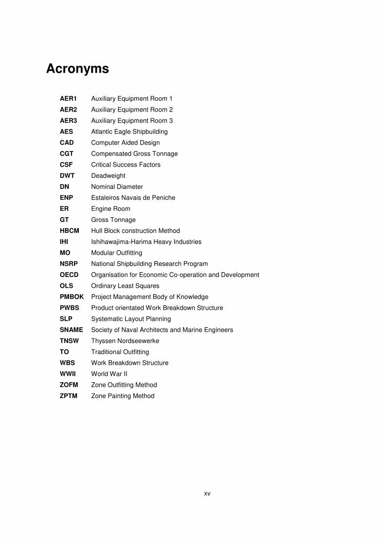
Acronyms

AER1 Auxiliary Equipment Room 1



AES Atlantic Eagle Shipbuilding

CAD Computer Aided Design

CGT Compensated Gross Tonnage

CSF Critical Success Factors

DWT Deadweight

DN Nominal Diameter

ENP Estaleiros Navais de Peniche

ER Engine Room

GT Gross Tonnage

HBCM Hull Block construction Method

IHI Ishihawajima-Harima Heavy Industries

MO Modular Outfitting

NSRP National Shipbuilding Research Program

OECD Organisation for Economic Co-operation and Development

OLS Ordinary Least Squares

PMBOK Project Management Body of Knowledge

PWBS Product orientated Work Breakdown Structure

SLP Systematic Layout Planning

SNAME Society of Naval Architects and Marine Engineers

TNSW Thyssen Nordseewerke

TO Traditional Outfitting

WBS Work Breakdown Structure

WWII World War II

ZOFM Zone Outfitting Method

ZPTM Zone Painting Method

2

1

1 Introduction

Contents

1.1 Dissertation’s scope of work ................................................................................................................. 4

1.2 Portuguese shipbuilding and ship repair ........................................................................................... 6

1.3 Haksolok ferry Vessel………………………...………………………………………………………………..8

4

Due to the competitiveness of the shipbuilding business environment, shipyards are always trying to

optimize their production efficiencies in terms of time, costs and quality, or in other words, to do more

with the same (or less) resources and obtaining better results.

One of the methodologies used to increase shipbuilding effectiveness is Modular Outfitting (MO)

approach.

Currently experts recommend the use of modular outfitting as a way of increasing efficiency and

competitiveness in shipbuilding comparatively to Traditional Outfitting (TO).

As defined by Rubesa [1], Ship modular outfitting is defined as “the installation of outfit systems and

components on a structural block or outfit unit prior to shipboard erection” and” Traditional Outfitting

process corresponds to on-board outfitting installation on a building berth before launching or on-

board after launching”.

Modular Outfitting methodology (as known as modular outfitting approach) allows the parallel

assembly of various outfitting systems, which has the potential to reduce the assembling Man-hours

and assembly time, when compared with traditional outfitting. [1]

1.1 Dissertation’s scope of work

The dissertation scope of work is to analyze a ferry vessel bilge’s fluid system assembly performed

by traditional outfitting production methodology, their inputs and outputs and to compare them with

the estimations of the equivalent parameters of fluid systems assembly performed by modular

outfitting production methodology.

A Ferry type vessel (Haksolok) for the Democratic Republic of East-Timor is under construction using

traditional outfitting at Atlantic Eagle Shipbuilding (AES) shipyard and is to be commissioned in 2018.

This study was made in collaboration with AES.

The data, concerning the assembly, installing and fitting by traditional outfitting used in this

dissertation, was mainly collected from the AES pre-existing documents, from technical drawings and

from field construction operations analysis. The data concerning modular outfitting alternative was

based on information referred in the existing literature and on information collected on site from the

production study (traditional outfitting data).

This study addresses three questions:

i. The workload differences between traditional outfitting on-board approach and modular

outfitting on-block approach.

ii. The potential layout changes required by the implementation of modular outfitting

processes versus the implementation of traditional outfitting process according to

Systematic Layout Planning (SLP) analysis.

iii. The risk management of modular outfitting approach implementation.

5

For each question specific objectives were defined.

Regarding the first question, the primary objective was to compare the Man-hours used in production

in the traditional on-board outfitting method with the Man-hours used in modular on-block outfitting

method.

This analysis was circumscribed to selected bilge piping zones of higher outfitting complexity for which

an increase in production efficiency could represent a significant decrease of workload.

The determinants considered for the workload calculation were the piping properties, namely:

dimension, shape, location and position inside of the ship. The methodology is explained in detail in

chapter 3.

Regarding the second question, the primary objective was to compare the distances and routes of the

existing layout versus the distances and routes of the modular outfitting adapted layout.

Regarding the third question, the primary objectives were to identify and manage the risks associated

to modular outfitting implementation, and to define the Critical Success Factors (CSFs) for effective

implementation of modular outfitting approach.

Each of the three questions was addressed in a dedicated chapter (chapter 3, 4 and 5) and all chapters

have a similar organizational structure.

6

1.2 Portuguese shipbuilding and ship repair

1.2.1 Portuguese Shipyards

Portuguese shipbuilding and ship repair business has several small/medium and one large shipyard.

The shipyards are briefly described below according to the information published on their websites.

West Sea - Estaleiros Navais de Viana do Castelo - located on the northern part of the Portuguese

coast, West Sea is now the biggest construction shipyard in Portugal, having great expertise and

experience in what concerns the shipbuilding activity.

West Sea yard has as infrastructures two drydocks with 203 and 127 meters of length.

Recently they were acquired by Martifer Metalic Constructions and have been building inland waters

cruise vessels for the river Douro and one naval ship.

Ship repair activities and construction of large steel structures are also performed in this shipyard.

Navalria - is a small shipyard located in Aveiro that used to be a fishing vessel focused shipyard. As

occurred with West Sea, Navalria was also acquired by Martifer Metalic Constructions and operates

in shipbuilding, ship repair and in the construction of large steel structures.

Navalria also repairs other smaller fishing vessels, working boats and historical ships. In terms of

facilities is important to mention the existence of a drydock, of a floating dock and of a syncrolift.

Estaleiros Navais de Peniche (ENP) - is a shipyard located in Peniche, that operates in shipbuilding

and ship repair of small size vessels. This yard gain reputation on the construction of composite

fishing vessels, although in recent years it has also built passenger ships and working boats.

Navalrocha - is a repair shipyard located in Lisboa. This shipyard belongs to a group of different

share holders and managed by ETE Group (Empresa de Trafego e Estiva) and has a great

experience in maintenance and repair works in all types of ships and can docks ships in the two

medium size graving docks.

NavalTagus - is a shipyard that also belongs to Grupo ETE and operates in shipbuilding and ship

repair of small dimension vessels. Concerning shipbuilding activity, this yard has launched a tug boat

in 2016. In repair business, NavalTagus, maintains inland waters barges, small dimension cargo ships

and passenger ships. This shipyard has two longitudinal ramps.

7

Lisnave Estaleiros Navais - is a southern shipyard located in Mitrena, Setubal. This is one of the

biggest repair shipyards in Europe. Its major income activity is ship repair.

Lisnave’s most remarkable assets are its dry docks. Having three large dimension drydocks: drydock

20, 21 and 22, with a respective length of over 400 meters, 350 meters and 300 meters.

Besides the main drydocks, Lisnave has three drydocks within an Hydrolift system with capacity to

receive up to Panamax type vessels.

Lisnave repairs around 100 vessels per year and has a regular client portfolio from more than 50

countries.

This enterprise was founded in 1961 and in the past used to operate first in Rocha Shipyard (now

explored by Naval Rocha) and from the early 1970’s until 1999 it had operated in Margueira’s yard.

From the early seventies to the turning of the XX century Lisnave repaired some of the largest vessels

operating worldwide including the French ULCCs (ultra large crude carrier) “Pierre Guillaumat” and

“Batillus” and including also the “Seawise Giant”, the largest vessel ever built.

Margueira’s yard had drydock 13 that during the 1970’s was considered the world’s large drydock,

could dock up to 1 000 000 tons of deadweight.

Nautiber - is a shipyard located on the shore of Guadiana River, near the city of Vila Real de Santo

Antonio, in Algarve. The shipyard’s areas of expertise are the shipbuilding and ship repair of vessels

built in fiberglass and wooden made. The major part of their vessel portfolio is building and repair

fishing vessels.

1.2.2 Atlanticeagle Shipbuilding (AES)

Atlanticeagle Shipbuilding (AES) is a construction and repair shipyard located near the city of

Figueira da Foz.

According to AES website (http://aeshipbuilding.com/pt/about-us/our-history/), this shipyard was

founded in 1947 under Estaleiros Navais do Mondego.

During the XX century this shipyard gain recognition especially due to the construction of fishing

vessels and passenger’s aluminium catamarans ferries. During the same century a large number of

other vessels besides fishing ships, were built including tug boats, general cargo boats, and others.

In 2012, the shipyard was acquired by new owners, having changed the name to Atlantic Eagle

Shipbuilding.

Nowadays several projects are being developed both on shipbuilding and ship repair, being one of the

most remarkable, the construction of a ferry vessel ”Haksolok” for the Autoridade da Região

Administrativa Especial de Oé-Cusse Ambeno, Timor Leste.

8

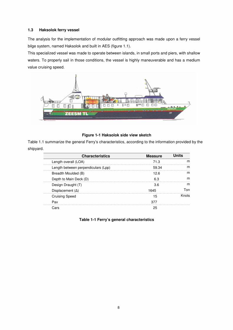
1.3 Haksolok ferry vessel

The analysis for the implementation of modular outfitting approach was made upon a ferry vessel

bilge system, named Haksolok and built in AES (figure 1.1).

This specialized vessel was made to operate between islands, in small ports and piers, with shallow

waters. To properly sail in those conditions, the vessel is highly maneuverable and has a medium

value cruising speed.

Figure 1-1 Haksolok side view sketch

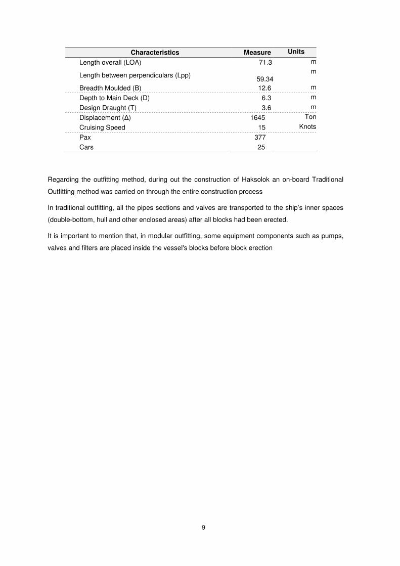
Table 1.1 summarize the general Ferry’s characteristics, according to the information provided by the

shipyard.

Characteristics Measure Units

Length overall (LOA) 71.3 m

Length between perpendiculars (Lpp) 59.34 m

Breadth Moulded (B) 12.6 m

Depth to Main Deck (D) 6.3 m

Design Draught (T) 3.6 m

Displacement (Δ) 1645 Ton

Cruising Speed 15 Knots

Pax 377

Cars 25

Table 1-1 Ferry’s general characteristics

9

Regarding the outfitting method, during out the construction of Haksolok an on-board Traditional

Outfitting method was carried on through the entire construction process

In traditional outfitting, all the pipes sections and valves are transported to the ship’s inner spaces

(double-bottom, hull and other enclosed areas) after all blocks had been erected.

It is important to mention that, in modular outfitting, some equipment components such as pumps,

valves and filters are placed inside the vessel's blocks before block erection

Characteristics Measure Units

Length overall (LOA) 71.3 m

Length between perpendiculars (Lpp) 59.34

m

Breadth Moulded (B) 12.6 m

Depth to Main Deck (D) 6.3 m

Design Draught (T) 3.6 m

Displacement (Δ) 1645 Ton

Cruising Speed 15 Knots

Pax 377

Cars 25

11

2

2 Behind State of Art

Contents

2.1 Preliminary concepts on ships life cycle ...........................................................................................12

2.2 Modular Outfitting ................................................................................................................................14

2.3 Systematic Layout Planning (SLP) .....................................................................................................21

2.4 Risk Management .................................................................................................................................27

13

This chapter introduces the main theoretical concepts about Modular Outfitting production

methodology, systematic layout planning and risk analysis, that will be applied in this study.

2.1 Preliminary concepts on ships life cycle

The ship’s life cycle theoretical concepts are introduced because they will be used to define the

identified risks of modular outfitting implementation Risk Analysis.

There are several ships’ project life cycle model descriptions in the literature. This study adapted the

Chapman and Ward [2] model that divides the project life cycle in to four major phases: conceptual

phase, planning phase, execution phase and termination phase (that is a risk management orientated

approach).

In this dissertation four ship’s life cycle phases were defined in accordance to the location of its

development

• Design Develop and Engineering phase corresponds to the merge of Conceptual phase

and Planning phase as they are developed in a ship design office

• Construction phase corresponds to Execution phase that is carried out on shipyard.

• Operation and Maintenance phase corresponds to Termination phase is directly executed

on board or on dock.

• Scrapping phase performed in a scrapping yard, was added to the project life cycle due to

its contribution to financial accounting (revenue).

Each of the vessel’s life cycle phases listed above has a specific impact on costs.

A visual representation of the vessel’s life cycle phases, it´s cost influence potential and the

proportional contribution to final costs is displayed in Figure 2.1.

14

Figure 2-1: MacGregor Ship’s cost influence curve according to life cycle phase

Adapted from Gomes Lopes [3]

Design Development and Engineering - Conceptual Phase

The decisions taken at this phase are key cost determinants, because during this phase the main

characteristics of the vessel are settled in order to meet the requirements of the ship mission and of

the stakeholders (shipowners and authorities).

This set of characteristics will define the ship namely in what concerns dimensions, capacity, speed

and shipyard construction support facilities. These decisions should be definitive. Any subsequent

changes (4) to theses fundamental characteristics will determine substantial additional costs.

Design Development and Engineering - Planning Phase

This phase includes designing of the vessel, planning of the strategy and allocation of the resources.

The designing of the vessel includes all the design steps, from basic design up to design evaluation and

vessel’s performance criteria.

The planning of the strategy consists of defining deadlines and milestones.

Finally, the resource allocation sub-phase incorporates the estimation of resources to be used, as for

example: the quantity of steel plates to be used for the structural blocks manufacturing.

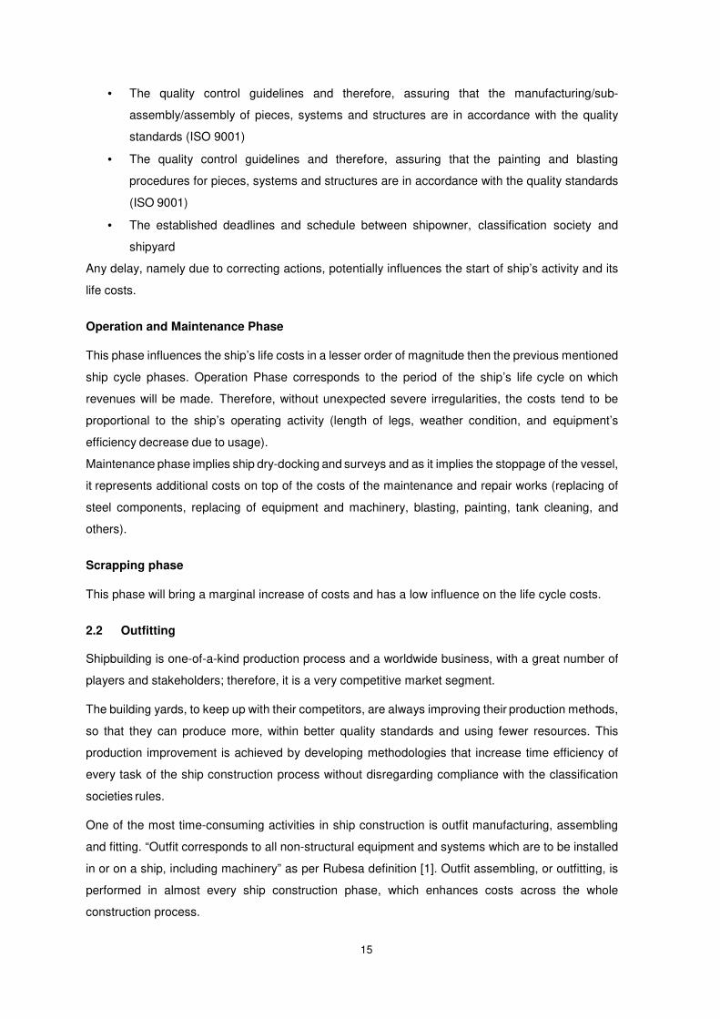
Construction Phase

It is a phase with an important cost impact magnitude that depends on the compliance requirements

regarding:

• The ship design phase decisions and with guidelines respecting the established scope of the

work

15

• The quality control guidelines and therefore, assuring that the manufacturing/sub-

assembly/assembly of pieces, systems and structures are in accordance with the quality

standards (ISO 9001)

• The quality control guidelines and therefore, assuring that the painting and blasting

procedures for pieces, systems and structures are in accordance with the quality standards

(ISO 9001)

• The established deadlines and schedule between shipowner, classification society and

shipyard

Any delay, namely due to correcting actions, potentially influences the start of ship’s activity and its

life costs.

Operation and Maintenance Phase

This phase influences the ship’s life costs in a lesser order of magnitude then the previous mentioned

ship cycle phases. Operation Phase corresponds to the period of the ship’s life cycle on which

revenues will be made. Therefore, without unexpected severe irregularities, the costs tend to be

proportional to the ship’s operating activity (length of legs, weather condition, and equipment’s

efficiency decrease due to usage).

Maintenance phase implies ship dry-docking and surveys and as it implies the stoppage of the vessel,

it represents additional costs on top of the costs of the maintenance and repair works (replacing of

steel components, replacing of equipment and machinery, blasting, painting, tank cleaning, and

others).

Scrapping phase

This phase will bring a marginal increase of costs and has a low influence on the life cycle costs.

2.2 Outfitting

Shipbuilding is one-of-a-kind production process and a worldwide business, with a great number of

players and stakeholders; therefore, it is a very competitive market segment.

The building yards, to keep up with their competitors, are always improving their production methods,

so that they can produce more, within better quality standards and using fewer resources. This

production improvement is achieved by developing methodologies that increase time efficiency of

every task of the ship construction process without disregarding compliance with the classification

societies rules.

One of the most time-consuming activities in ship construction is outfit manufacturing, assembling

and fitting. “Outfit corresponds to all non-structural equipment and systems which are to be installed

in or on a ship, including machinery” as per Rubesa definition [1]. Outfit assembling, or outfitting, is

performed in almost every ship construction phase, which enhances costs across the whole

construction process.

16

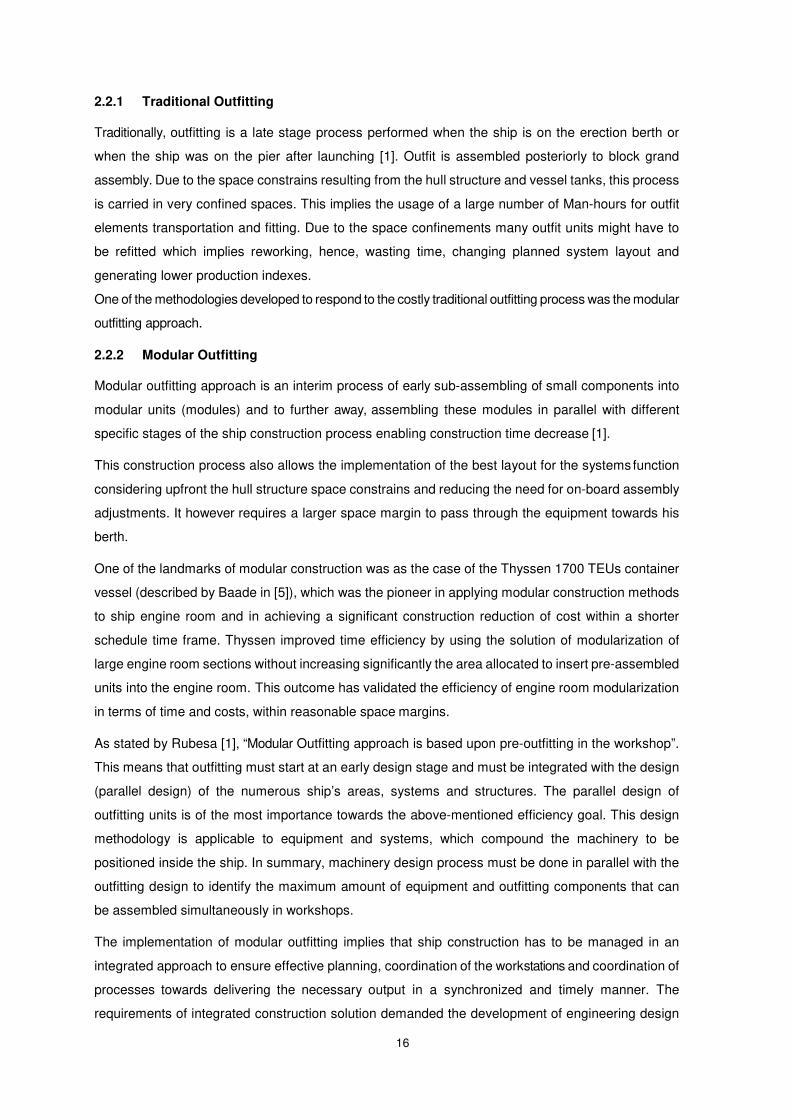
2.2.1 Traditional Outfitting

Traditionally, outfitting is a late stage process performed when the ship is on the erection berth or

when the ship was on the pier after launching [1]. Outfit is assembled posteriorly to block grand

assembly. Due to the space constrains resulting from the hull structure and vessel tanks, this process

is carried in very confined spaces. This implies the usage of a large number of Man-hours for outfit

elements transportation and fitting. Due to the space confinements many outfit units might have to

be refitted which implies reworking, hence, wasting time, changing planned system layout and

generating lower production indexes.

One of the methodologies developed to respond to the costly traditional outfitting process was the modular

outfitting approach.

2.2.2 Modular Outfitting

Modular outfitting approach is an interim process of early sub-assembling of small components into

modular units (modules) and to further away, assembling these modules in parallel with different

specific stages of the ship construction process enabling construction time decrease [1].

This construction process also allows the implementation of the best layout for the systems function

considering upfront the hull structure space constrains and reducing the need for on-board assembly

adjustments. It however requires a larger space margin to pass through the equipment towards his

berth.

One of the landmarks of modular construction was as the case of the Thyssen 1700 TEUs container

vessel (described by Baade in [5]), which was the pioneer in applying modular construction methods

to ship engine room and in achieving a significant construction reduction of cost within a shorter

schedule time frame. Thyssen improved time efficiency by using the solution of modularization of

large engine room sections without increasing significantly the area allocated to insert pre-assembled

units into the engine room. This outcome has validated the efficiency of engine room modularization

in terms of time and costs, within reasonable space margins.

As stated by Rubesa [1], “Modular Outfitting approach is based upon pre-outfitting in the workshop”.

This means that outfitting must start at an early design stage and must be integrated with the design

(parallel design) of the numerous ship’s areas, systems and structures. The parallel design of

outfitting units is of the most importance towards the above-mentioned efficiency goal. This design

methodology is applicable to equipment and systems, which compound the machinery to be

positioned inside the ship. In summary, machinery design process must be done in parallel with the

outfitting design to identify the maximum amount of equipment and outfitting components that can

be assembled simultaneously in workshops.

The implementation of modular outfitting implies that ship construction has to be managed in an

integrated approach to ensure effective planning, coordination of the workstations and coordination of

processes towards delivering the necessary output in a synchronized and timely manner. The

requirements of integrated construction solution demanded the development of engineering design

17

and of supporting equipment and software, a more sophisticated work scheduling and more complex

system of standardized operating procedures regarding outfit construction and assembly. To comply

with the demands of integrated construction process and modular outfitting approach, nowadays the

usage of simulation software has been widespread along shipyards [7], preventing errors, rework

and added costs.

2.2.2.1 Modular Outfitting Evolution and Implementation

Modular outfitting methodologies resulted from several improvements regarding organizational

theories, equipment and materials as well as supporting design systems derived from the creation of

Computer Aided Design (CAD) software, simulation software and management software.

Prior to World War II (WWII) new kind of practices started to be developed and were implemented

afterwards [8] from the production revolution induced by WWII on. The most remarkable improvement

among the new practices, such as the introduction of standardized procedures and design

simplification, was the construction of ships by using block assembling. This practice was

implemented in the US by Henry Kaiser’s introduction of Group Technology. Further away Helmer

Hann, a former Kaiser’s employee, took these practices to a Japanese Industry enterprise named

Industries Ishihawajima-Harima Heavy Industries (IHI). Based on the acquired know-how, IHI not only

implemented these practices into their manufacturing systems, but also further developed and

changed the concept of shipbuilding, creating a new work organization called Production Work

Breakdown System (Product orientated Work Breakdown Structure (PWBS)). This system was

implemented in the decades of 1960 and 1970 and during this period IHI had outstanding results,

producing over 2000 ships.

On the year of 1970, in the US, the National Shipbuild Research Program (National Shipbuilding

Research Program (NSRP)) was created. During that decade, in order to exchange information and

to promote technological improvements, this entity established a connection between the US and

Japanese shipbuilders. In 1979, as a result of this cooperation, a book of reference named “Outfitting

Planned” based on the PWBS. During the following decade NSRP improved the procedures of PWBS

and published a vast amount of literature related to integrated construction (which includes outfitting).

During the 1990’s several shipyards tried to improve the results obtained from the US-Japan

shipbuilding joint venture and discovered several different new types of production methods.

In 1991, as previously mentioned, Thyssen Nordseewerke (TNSW) built the 1700 TEU container

vessel that used the modular solution [5], for the piping system of the engine room and that triggered

the need for an integrated construction approach in order to enable the assembly of the modular

outfitting units without under space crashing and potential rework. This was the first time that this

type of procedure was applied [8]. During the 2000’s decade fully integrated steel and outfitting

construction were developed.

2.2.2.2 Integrated Shipbuilding Process

Integrated construction means that each process can be divided into interim parts that might be

18

combined at an optimum stage of the construction process [9], which improves the construction rate

and reduces the number of conflicts and rework processes.

Modular outfitting approach is an internal sub process of the integrated shipbuilding process, which

is widely used by the most advanced shipyards. Figure 2.2 shows a modern shipyard layout and the

integrated outfitting assembly workflow.

Altic [9]

Integrated construction relies on the organization according to PWBS method that consists in a

method of breakdown of the entire ship construction process into smaller and interim sub-processes

gathered by type of technology among similar systems. This breakdown into interim sub processes

enables the disentangling of activities that can be performed in parallel, instead of being performed

sequentially.

Another fundamental concept is zone-orientated design. According to the NSRP [10], the most important

principle in zone orientated design is: ”…that material which is first assigned by function (system) is

reassigned geographically” to excel the workflow. This methodology aims to increase the productivity

indexes by centralizing all the work force and resources of a certain technological group on the same

facility zone and by managing in parallel multiple technological groups. This approach intends to

decrease the distance between materials and working stations, hence, it removes wasted steps and

generates an agile workflow and consequentially enhances the production indexes. It also reduces

barriers between group management entities and workers, improving communication among and

across work teams. It is crucial to mention that every process of integrated construction is classified

according to a PWBS code that creates a set of references to identify and organize all the working

processes and the manufactured pieces.

MO

Assembly zone

Figure 2-2: Integrated outfitting assembly

MO

Assembly zone

19

According to Society of Naval Architects and Marine Engineers (SNAME)’s ship production book [11]

there are three different integrated shipbuilding sub processes:

i. Hull Block Construction Method (HBCM)

ii. Zone Outfitting Method (ZOFM)

iii. Zone Painting Method (ZPTM)

The Hull Block Construction Method and the Zone Outfitting Method are the most relevant sub

processes for the scope of this thesis.

The goal of HBCM is to divide the ship structure manufacturing process into optimum blocks.

Optimum blocks are designed considering structural elements plus outfitting components plus

painting.

These three sub processes will be executed independently from one another and the quality of the

block optimization will depend on the effective coordination between these parallel sub processes.

Each of these sub processes is subdivided into lower level processes, which are defined according to

the similarity of components regarding volume, weight and shape. This likeliness is important

because it will sharpen the assembly of parts/components into modularized units.

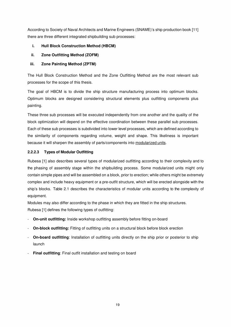
2.2.2.3 Types of Modular Outfitting

Rubesa [1] also describes several types of modularized outfitting according to their complexity and to

the phasing of assembly stage within the shipbuilding process. Some modularized units might only

contain simple pipes and will be assembled on a block, prior to erection; while others might be extremely

complex and include heavy equipment or a pre-outfit structure, which will be erected alongside with the

ship’s blocks. Table 2.1 describes the characteristics of modular units according to the complexity of

equipment.

Modules may also differ according to the phase in which they are fitted in the ship structures.

Rubesa [1] defines the following types of outfitting:

- On-unit outfitting: Inside workshop outfitting assembly before fitting on-board

- On-block outfitting: Fitting of outfitting units on a structural block before block erection

- On-board outfitting: Installation of outfitting units directly on the ship prior or posterior to ship

launch

- Final outfitting: Final outfit installation and testing on board

20

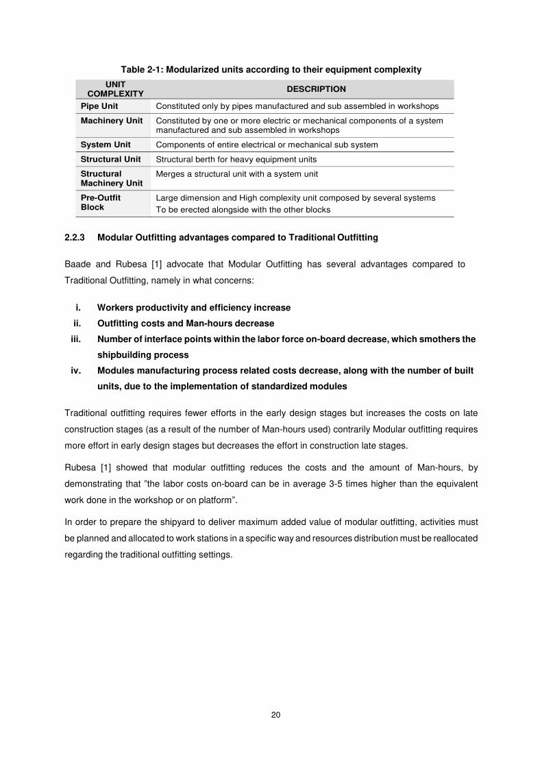
Table 2-1: Modularized units according to their equipment complexity

2.2.3 Modular Outfitting advantages compared to Traditional Outfitting

Baade and Rubesa [1] advocate that Modular Outfitting has several advantages compared to

Traditional Outfitting, namely in what concerns:

i. Workers productivity and efficiency increase

ii. Outfitting costs and Man-hours decrease

iii. Number of interface points within the labor force on-board decrease, which smothers the

shipbuilding process

iv. Modules manufacturing process related costs decrease, along with the number of built

units, due to the implementation of standardized modules

Traditional outfitting requires fewer efforts in the early design stages but increases the costs on late

construction stages (as a result of the number of Man-hours used) contrarily Modular outfitting requires

more effort in early design stages but decreases the effort in construction late stages.

Rubesa [1] showed that modular outfitting reduces the costs and the amount of Man-hours, by

demonstrating that ”the labor costs on-board can be in average 3-5 times higher than the equivalent

work done in the workshop or on platform”.

In order to prepare the shipyard to deliver maximum added value of modular outfitting, activities must

be planned and allocated to work stations in a specific way and resources distribution must be reallocated

regarding the traditional outfitting settings.

UNIT COMPLEXITY

DESCRIPTION

Pipe Unit Constituted only by pipes manufactured and sub assembled in workshops

Machinery Unit Constituted by one or more electric or mechanical components of a system manufactured and sub assembled in workshops

System Unit Components of entire electrical or mechanical sub system

Structural Unit Structural berth for heavy equipment units

Structural Machinery Unit

Merges a structural unit with a system unit

Pre-Outfit Block

Large dimension and High complexity unit composed by several systems

To be erected alongside with the other blocks

21

Gomes Lopes [3] illustrates the difference of planning and resources allocation between traditional

outfitting and modular outfitting depending on outfitting process phase, in two charts (figures 2.3 and

2.4).

Gomes Lopes [3]

Figure 2-4: Resources (line width scale) allocated to MO assembly

Gomes Lopes [3]

Besides the positive points mentioned above, Baade [5] describes another advantage of modular

outfitting is the capacity to simultaneously perform work on several systems in parallel, in a synchronized

way.

An example of parallel work is the case where steel blocks near the engine room area are assembled at

the same time as the outfitting modules to be fitted in those very same blocks.

Figure 2-3: Resources (line width scale) allocated to TO assembly

22

Even though, modular outfitting has multiple advantages, according to Rubesa there are also some

disadvantages, such as:

- Design freedom decrease due to the space constraints on ship’s inner parts

- Inner space requirements increase

- Heavier outfitting structures (due to modules structures) than in traditional outfitting

- Precision requirements of detail engineering substantially increase to avoid rework

2.3 Systematic Layout Planning (SLP)

As mentioned in the introductory chapter, one of the questions to be addressed in this dissertation

regards the necessary layout changes required by the implementation of modular outfitting processes

versus the implementation of traditional outfitting.

To answer this question, the Muther systematic layout planning method [12] was selected as the layout

arrangement tool to be handled.

R. Muther defines [12] Systematic Layout Planning as a layout design methodology that aims towards

the facilitation of the manufacturing process.

When solving a layout problem, designers will face the following questions:

- “WHAT” is going to be made/produced? (Product/Material)

- “HOW MUCH” of each item is going to be manufactured? (Quantity/Volume)

- “HOW” is it going to be produced? (Routing/Process Sequence).

(At this step production guidelines are defined, concerning flow sheets, process sheets,

equipment’s lists and others)

- “WITH WHAT” is it going to be produced? (Supporting Services)

(This includes all the auxiliary equipment related to the main production system)

- “WHEN” will it be produced? (Time)

This step is deeply related with the scheduling of the production activity.

Layout design is a continuous adapting process according to existing resources and limitations.

These five elements are the foundation of the PQRST key to unlock layout problems and are

represented in figure 2.5.

Muther [12]

P PRODUCT - MATERIAL

WHAT is to be produced?

S SUPPORTING SERVICES

WITH WHAT support will

production be backed?

HOW will it (they) be produced?

HOW MUCH of each item will be

made?

WHEN will items be produced?

R ROUTING – PROCESS SEQUENCE

T TIME - TIMINGQ QUANTITY - VOLUME

W H Y

Figure 2-5: PQRST key to unlock layout problems

23

2.3.1 Phases of layout planning

There are three primordial principles that constitute the backbone of a layout:

- Relationships - indicating the strength of the connection between things

(Example: Relationship between steel shop and panel line)

- Space - indicating the physical dimensions of a thing

- Adjustment - optimizing arrangement to allow things to fit more properly

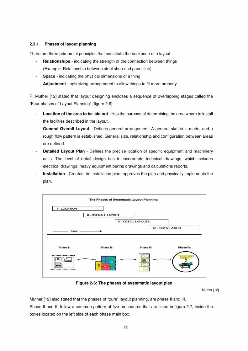
R. Muther [12] stated that layout designing encloses a sequence of overlapping stages called the

“Four phases of Layout Planning” (figure 2.6).

- Location of the area to be laid out - Has the purpose of determining the area where to install

the facilities described in the layout.

- General Overall Layout - Defines general arrangement. A general sketch is made, and a

rough flow pattern is established. General size, relationship and configuration between areas

are defined.

- Detailed Layout Plan - Defines the precise location of specific equipment and machinery

units. The level of detail design has to incorporate technical drawings, which includes

electrical drawings; heavy equipment berths drawings and calculations reports.

- Installation - Creates the installation plan, approves the plan and physically implements the

plan.

Figure 2-6: The phases of systematic layout plan

Muther [12]

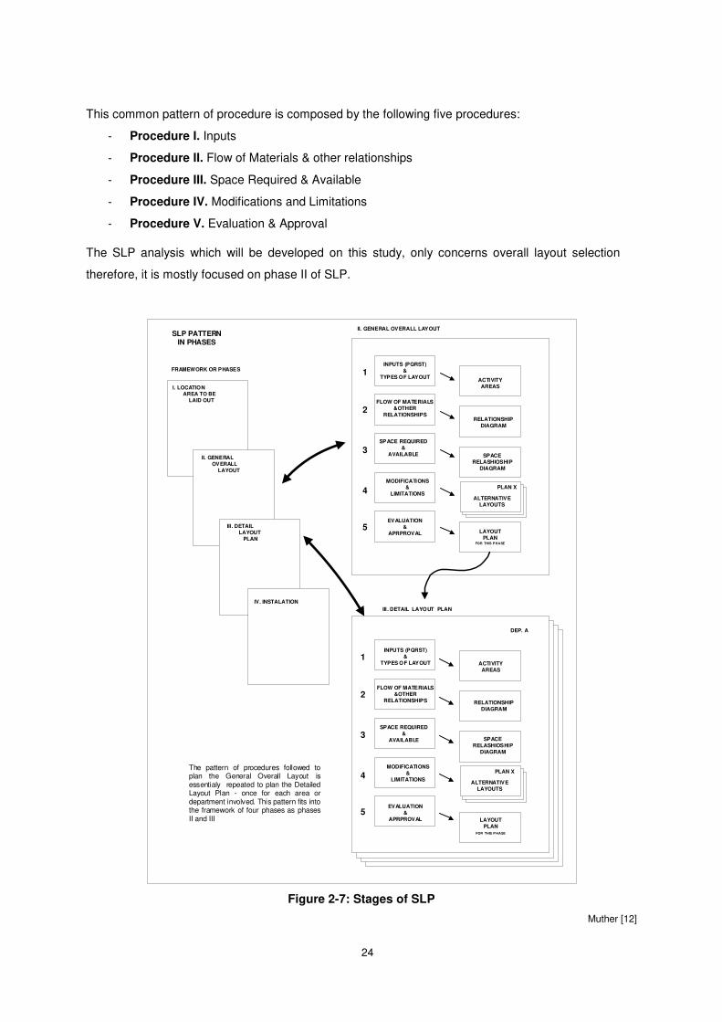
Muther [12] also stated that the phases of “pure” layout planning, are phase II and III.

Phase II and III follow a common pattern of five procedures that are listed in figure 2.7, inside the

boxes located on the left side of each phase main box.

24

This common pattern of procedure is composed by the following five procedures:

- Procedure I. Inputs

- Procedure II. Flow of Materials & other relationships

- Procedure III. Space Required & Available

- Procedure IV. Modifications and Limitations

- Procedure V. Evaluation & Approval

The SLP analysis which will be developed on this study, only concerns overall layout selection

therefore, it is mostly focused on phase II of SLP.

Figure 2-7: Stages of SLP

Muther [12]

SLP PATTERNIN PHASES

FRAMEWORK OR PHASES

I. LOCATION AREA TO BE LAID OUT

II. GENERAL OVERALL LAYOUT

III . DETAIL LAYOUT PLAN

IV. INSTALATION

INPUTS (PQRST)&

TYPES OF LAYOUT

FLOW OF MATERIALS&OTHER

RELATIONSHIPS

EVALUATION &

APRPROVAL

SPACE REQUIRED &

AVAILABLE

MODIFICATIONS&

LIMITATIONS

RELATIONSHIPDIAGRAM

SPACERELASHIOSHIP

DIAGRAM

ACTIVITYAREAS

LAYOUTPLAN

FOR THIS PHASE

II. GENERAL OVERALL LAYOUT

1

2

3

4

5

1

2

3

4

5

RELATIONSHIPDIAGRAM

SPACERELASHIOSHIP

DIAGRAM

ACTIVITYAREAS

ALTERNATIVELAYOUTS

LAYOUTPLAN

FOR THIS P HASE

INPUTS (PQRST)&

TYPES OF LAYOUT

FLOW OF MATERIALS&OTHER

RELATIONSHIPS

EVALUATION &

APRPROVAL

SPACE REQUIRED &

AVAILABLE

MODIFICATIONS&

LIMITATIONS

DEP. A

PLAN X

ALTERNATIVELAYOUTS

PLAN X

III . DETAIL LAYOUT PLAN

The pattern of procedures followed to plan the General Overall Layout is essentialy repeated to plan the Detailed Layout Plan - once for each area or department involved. This pattern fits into the framework of four phases as phases II and III

25

2.3.2 Layout Developments

To create and develop the layout, each of the SLP procedures must deliver specific outputs, as stated

below:

- Procedure I - identification of the needed activities to be developed and the space requirements

- Procedure II - perception of the relationships between activities and material flows

- Procedure III – definition of spaces required to accommodate each activity and their relationship

and interface;

- Procedure IV - adjustments that enable realist plan implementation or potential improvements

- Procedure V - final layout selection among several possible alternatives, taking in consideration

added values and cost, that once approved closes phase II

Layout development tools are used to complete procedure II and III.

There are three fundamental tools that will enable a systematic data collection, a user-friendly

representation of activities flows, activities and space relationships, and that will also support the

decision-making process of selecting the best layout among the several alternatives generated.

These tools are: the Relationship Chart, the Flow/Activity Relationship Diagram and the Space

Diagram.

2.3.2.1 Relationship Chart

This tool provides the basis for the Flow/Activity diagram and is also an input for the space

relationship diagram.

The Relationship Chart plots the existing relationships between the existing activities in a production

system. It rates the activities closeness in a scale from A to X (A, E I, O, U and X), being A an

absolutely necessary relationship and X a non- desirable relationship (figure 2.8).

RECEPTION PARK

CUTTING FACILITY

OUTFITTING SHOP

PIPE SHOP

BLASTING AND PAINTING SHOP

MECHANICAL AND ELECTRICITY SHOP

CARPENTER SHOP

PANEL LINE

STEEL SHOP

BLOCK MANUFACTURING PARK

PIER

CONSTRUCTION RAMP

35

31

30

29

28

27

17

11

10

4

3

1

VO WEL

LETTE R

A

E

I

O

U

CLOSE NESS RATI NG

ABSO LU TELY

NE CES SARY

ESPECI ALLY

IM PORTANT

IM PORTANT

O RD INA RY

UN IM PORTANT

COL OR

COD E

A

E

I

O

U

U

U

E

A

O

U

U

E

U

E

A

A

E

I

O

U

A

E

I

O

U

A

I O

U

A

E

I

OU

A

E

O

U

A

E

O

U

UU

U

U

U

E

E

EAA

AU U

U

U

A

OO

O

O

OO

O

Figure 2-8: Example of relationship chart

26

2.3.2.2 Space Relationship Diagram

This diagram provides a visual representation that combines activities relationship and work flows.

This type of diagram uses standardized ANSI symbols to represent the sort of activity performed and

to represent the relationship closeness. It consists in a representation of the activity relationships and

flows, superimposed on the space layout.

This diagram is based upon the relationship chart and the flow activity diagram combined with the

space requirements and availability. However, instead of using the ANSI symbols to represent an

activity it uses a representation of the infrastructures by scale (each site will be represented according

to its area) and intersects this new representation with the flow lines plotted in the flow relationship

diagram (annex B).

In the dissertation’s SLP study, the Relationship Chart and the Space Relationship Diagram are the

most relevant outputs for layout selection.

2.3.3 Layout Selection and Readjustments

The space relationship diagram provides several alternative layouts that will be compared in order to

select the best one.

According to Muther [12] the selection of a new layout has to be made upon the three methods:

i. Factor analysis rating

ii. Advantages and disadvantages weigh

iii. Cost comparison

Once the final layout is selected it must be rearranged to accommodate requirements of reality

conditions.

It is to be noted that on this dissertation the questions concerning implementation of modular outfitting

will address layout adjustment and layout selection processes.

2.3.3.1 Layout Selection and Readjustment - Factor analysis rating

The multiplicity of factors that can affect a layout makes its analysis a complex problem. In order to

overcome this complexity, a process of problem breakdown, named Factor Analysis, was developed.

Thus, as in every complex engineering problem, it follows the methodology of dividing the problem

into several smaller problem units that can be more easily managed. According to Muther [12] “The

Factor Analysis method follows the engineering concept of breaking down the problem into its

elements and analyzing each one”.

Factor Analysis methodology has the following steps:

i. List of all the meaningful factors to determine the layout to be implemented

ii. Balance the relative weight of each of the previous mentioned factors

iii. Rate the alternative layouts against each factor in a sequential way

iv. Compare the total value of all the alternative designed layouts

27

2.3.3.2 Layout Selection and Readjustment - Advantages versus disadvantages weigh

This method allows the designer to clearly expose some key factors that should be taken in

consideration in the layout selection process.

The weight of the exposed advantages or disadvantages is rated according to a vowel and numerical

code rating (table 2.2).

This rating supports the designer recommendation regarding the possible adjustments of the layout

design.

Table 2-2: (Dis)Advantages letter and numerical coding

RATING CODE AND VALUES

Vowel Coding Description of the rate Numerical Value

A Almost Perfect – (Excellent) 4

E Especially Good – (Very Good) 3

I Important Results Obtained – (Good) 2

O Ordinary Results Provided – (Fair) 1

U Unimportant Results – (Poor) 0

X Not Acceptable – (Not Satisfactory) ?

R.Muther [12]

2.3.3.3 Layout Selection and Readjustment - Cost Comparison

The estimation of the overall costs must be based on the largest possible amount of available data in

order to allow an accurate cost analysis to base the layout selection decision.

Cost comparison between layout alternatives is made upon the following parameters:

i. Flow Index

ii. Transport Work

iii. Cost estimation of material handling

Flow index consists on the analysis of the layout efficiency in terms of workflow.

As the workflow depends on the distances between work stations and the activities relationships, this

parameter is defined by analyzing the existing distance between activity locations and by analyzing

activities closeness. Thus, SLP outputs, such as space relationship diagram, are critical tools for this

analysis.

Transport work is defined by Muther [12],”..., as intensity (of flow) times distance...”. When designing

a layout, it is necessary to estimate the costs of material handling/transport.

At this stage several flow relations were already defined and therefore both the paths to be used and

their length are already known. Thus, multiplying distance by a two-way trip it is possible to estimate

with satisfactory accuracy the total length covered.

Cost estimation of the definitive material handling, according to the already mentioned author

28

[12], implies not only the detailed definition of the working stations and the carrying equipment, as

well as its working cost, but also the decision on where to place the handling terminals and the

calculation of the distances between the station to pick-up and the station set-down.

The selection layout decision should also take in consideration cost comparison and differences in

added value provided by each of the alternative layouts.

2.4 Risk Management

Decision making process implies problem analysis that includes risk estimation. Risk response plans

should be developed in order to manage the identified risks. To implement a new outfitting installation

method in the production line of an existing shipyard, the risk of unmet expectations and its potential

additional costs have to be accessed.

The management of the project should also be based on the identification and prioritization of the

favorable factors that are key to obtain results according to its goals.

In the introductory chapter, one of the three formulated questions of the dissertation scope of work,

concerned modular outfitting implementation risk management.

Guedes Soares [13], has defined risk as “... the expected value of the process consequences per unit of

time” (translated from Portuguese).

The Project Management Body of Knowledge (2008 PMBOK) [14] states that: “Risk management is the

systematic process of identifying, analyzing and responding to project risk. It includes maximizing the

probability and consequences of positive events and minimizing the probability and consequence of

adverse events to project objectives”

29

The six risk management major processes are defined as per PMBOOK [14,ch11 ]:

i. Risk Managing Planning - selects the way to approach and plan the risk management

activities for a project

ii. Risk Identification - determines the type of risks that can affect a project and itemizes their

characteristics

iii. Qualitative Risk analysis - executes a qualitative analysis of risks and conditions to prioritize

their implications on the project’s goals.

iv. Quantitative Risk analysis - measures the probability and consequences of risks and

reckoning their effect for the project goals.

v. Risk Response Planning - develops procedures and techniques to magnify opportunities

and decrease threats to the project’s goals

vi. Risk Monitoring and Control - monitors residual risk, identifies new risk, executes risk

reduction plans, and appraises their effectiveness during the project life cycle

Concerning risk analysis, Guedes Soares [13] stated that it is a method that aims to determine the

existing risk associated with a given process or system. There are two related approaches to risk

analysis: qualitative and quantitative. Both were defined above but due to the scope of this thesis,

only the qualitative approach will be detailed.

One useful risk analysis tool is the likelihood-impact table/matrix. This matrix displays for each

identified risk, a risk score based on the estimated risk impact and on the estimated risk likelihood.

This risk score is obtained by the multiplication of the weighted value of impact factor by the weighted

value of likelihood factor. These weighted values are displayed in a scale from 1 to 5.

The risk scores results are displayed in a Probability-Impact table and their magnitude is represented

by a color code of a four colors sequential scale.

According to PMBOK [14], the risk response planning can be defined as “the process of developing

options and determining actions to enhance opportunities and reduce threats to the project’s

objectives”. Thus, the purpose of risk response is to decide which strategies should be taken to

contain threats (or increase opportunities).

The adopted risk response strategies are the following:

i. Avoidance - this strategy involves the need to revise the project to eradicate the risk. Usually

this strategy is used in risk with high impact and high likelihood.

ii. Transference - this strategy implies the deviation of the risk to a third party. This does not

eliminate the risk but shifts the responsibility. Transferring is used in risk with high impact and

medium likelihood.

iii. Mitigation - this strategy looks for the reduction of the consequences of an adverse risk to

an acceptable limit. It is applied on risk with medium impact and medium/high likelihood.

iv. Acceptance - this strategy is characterized by the recognition of low impact risk and

therefore, it can be accepted in the project without adjustments. This strategy is used for low

impact risks and for low and medium likelihood factors.

30

Having described the risk response strategies, the next step of risk management processes is the

creation and implementation of risk monitoring and risk control plans. This step is not to be developed

in this dissertation, although it could be developed in future studies.

To estimate the impact factors of the identified risks, Guedes Soares and Gomes Lopes [15]

suggested a methodology. This methodology quantifies every identified risk in terms of:

- Quality

- Cost

- Time

These parameters are individually quantified in a scale from 1 to 5, in which “1” stands for reduced

impact and “5” for high impact. Once every parameter is quantified, all the values concerning each risk

are summed.

It is to be noted that the study to be performed in chapter 5 will be based upon the risk identification

process, the risk qualitative analysis and the risk response planning.

Success Factors, according to Rockart and Bullen [16], are circumstances that lead to outcomes

that guarantee favorable and prosperous performance for an individual, a group or an organization.

Critical Success Factors are the decisive factors in which it is crucial to obtain positive results, in

order to achieve the established objectives and to achieve success.

In this dissertation, contiguous to the risk management analysis, a sub chapter of Critical Success

Factors was developed for the construction of a vessel in a medium size shipyard.

31

3

3 Comparison between man hours

using Traditional Outfitting and

Modular Outfitting

Contents

3.1 Problem modeling …………………………………………………………………………………………………………32

3.2 Analysis Methodology.......................................................................................................................................... 32

3.3 Results and Analysis............................................................................................................................................ 44

33

This chapter develops and analyzes the differences in terms of effectiveness (Man-hours) between a

traditional outfitting method and a modular outfitting method. This study only includes the parts of the

ship’s bilge system.

3.1 Problem Modeling

The scope of this chapter is to describe the comparison of effectiveness between traditional on-board

outfitting method and the modular outfitting method, regarding work load expressed in number of

Man-hours, allocated to the installing and fitting part of a bilge system composed by multiple pipe

sections, valves and pumps. (figure 3.5 and figure 3.6)

The workload data of the system’s section was obtained from the technical drawings provided by

AES, regarding bilge system pipeline isometric and bilge system lines diagram.

The Man-hours used to assemble each pipe section depended on factors such as dimension,

shape, location and position inside of the ship.

3.2 Analysis Methodology

This section will describe the methodology used for the study of the implementation of modular

outfitting methodology to the bilge piping system.

In a vessel there are several piping systems with a multiplicity of different components. For the study

purpose, due to this extensive number of systems and components, it was defined that the production

analysis would only be applied to the ship’s bilge system.

Modular outfitting can only be used in selected groups of the pipe system that for the purpose of the

study will be called modular outfitting zones, as per section 3.2.1.

According to Rubesa [1], Modular outfitting, when compared to traditional on-board outfitting, can

have a potential impact on the necessary assembly workload because as already mentioned in

subsection 2.2.3, it can reduce assembly time down to 3 to 5 times.

In this study the pipe sections of bilge system, suitable for the modular outfitting method, were

selected upfront according to predefined criteria described in 3.2.1.

Subsequently the Man-hours actually spent on the selected sections of the bilge system were

collected on field, then they were computed for both traditional outfitting and modular outfitting and

finally they were compared.

34

3.2.1 Selection of the bilge system zones for Modular Outfitting implementation

The focus of this selection aimed to identify the most complex assembly outfitting procedures, that

are the most time consuming, for which the return of an increase of production efficiency could be

translated into a decrease of the workload (expressed in Man-hours).

Two complexity parameters were empirically defined:

- Highest quantity of elements per unit of space (m3)

- Space availability for fitting an outfitting module

The first step of the selection was to identify on the bilge’s system isometric drawing the areas with the

highest density of elements. Three areas were pinpointed.

The second step was to verify in the digital model of the vessel’s system, provided by AES, if these three

areas were the denser in terms of elements and if the space available was enough to fit a module.

The third step was to confirm the parameters on-board.

Having these parameters in consideration, 3 zones were selected as being suitable for modular outfitting

implementation:

- Zone 1- Located inside the Engine Room (ER) adjacent to the engine room’s aft bulkhead (frame 23)

- Zone 2 - Located inside the ER adjacent to the engine room’s forward bulkhead (frame 39/40)

- Zone 3 - Located inside the Auxiliary Equipment Room 1 (AER1) forward to the engine room’s forward

bulkhead (frame 43)

The number of pipe sections in each Zone are displayed in table 3.1 and the specific section’s properties

are displayed in annex A.

Every system element identified was coded according to the Work Breakdown Structure (WBS)

methodology (figure 3.1) that defined 4 digit levels, where:

- the 1st digit is related to the compartment of the ship where the elements are placed

- the 2nd digit is related to the zone of the ship’s compartment Modular Outfitting Zone)

- the 3rd digit is related with the element number

- the 4th digit is related with the sub-element number

Zone # of elements Location

1 14 Engine Room (near engine room aft bulkhead; FR #23)

2 27 Engine Room (near engine room fwd bulkhead; FR #39/40)

3 19 Auxiliary Equipment Room 1 (FR #43)

Table 3-1: Defined zones for Modular Outfitting, number of sections and location

35

-

Figure 3-1: Example that illustrates the 4 levels of the WBS codification used

3.2.2 Calculation of outfitting assembly Man-hours

The calculation of the potential Man-hours gain of the bilge system assembly and fitting resulting from

the comparison between modular outfitting and traditional outfitting required the assessment of the

workload of both outfitting methods.

3.2.2.1 Traditional outfitting assembly Man-hours variables

The Man-hours values depend on four main factors:

- Pipe Dimension

- Pipe Shape

- Equipment Installing

- Pipe Location (inside the ship’s compartments)

Pipe Dimension is its major determinant. Figure 3.2 represents these factors composition.

W.B.S.

PIPE SUBSECTION

X X X X

VESSEL’S COMPARTMENT

1 - Engine room

2 - Aux. Equipment Room 1

MO ZONE

1 - Engine room FR #43

2 - Engine room FR #39/40

3 - Aux. Equipment Room 1 FR#43

PIPE SECTION

W.B.S. EXAMPLE

1 2 1 3

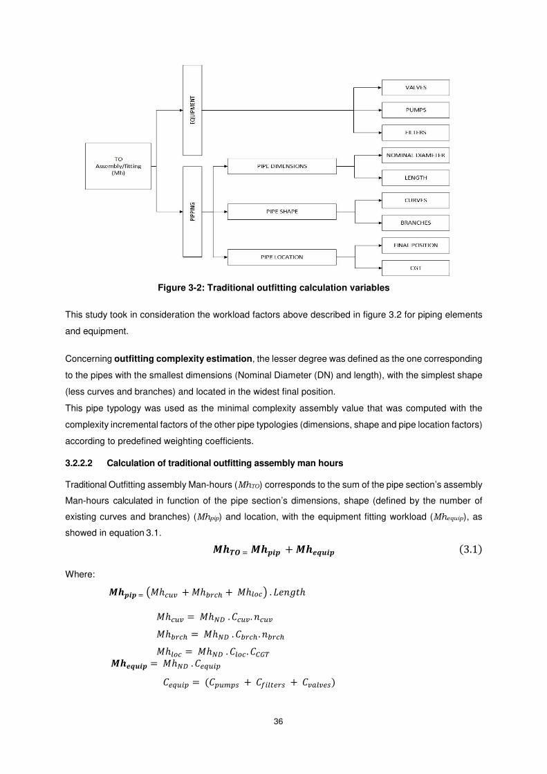
36

Figure 3-2: Traditional outfitting calculation variables

This study took in consideration the workload factors above described in figure 3.2 for piping elements

and equipment.

Concerning outfitting complexity estimation, the lesser degree was defined as the one corresponding

to the pipes with the smallest dimensions (Nominal Diameter (DN) and length), with the simplest shape

(less curves and branches) and located in the widest final position.

This pipe typology was used as the minimal complexity assembly value that was computed with the

complexity incremental factors of the other pipe typologies (dimensions, shape and pipe location factors)

according to predefined weighting coefficients.

3.2.2.2 Calculation of traditional outfitting assembly man hours

Traditional Outfitting assembly Man-hours (MhTO) corresponds to the sum of the pipe section’s assembly

Man-hours calculated in function of the pipe section’s dimensions, shape (defined by the number of

existing curves and branches) (Mhpip) and location, with the equipment fitting workload (Mhequip), as

showed in equation 3.1.

�� + �� 3.1� Where:

�� ℎ�� + �ℎ�� + �ℎ�� . �� !"ℎ �ℎ�� = �ℎ$% . &��. �� ℎ�� = �ℎ$% . &�� . �� ℎ�� = �ℎ$% . &�� . &'()

�� = �ℎ$% . &*+�,- &*+�,- = &-�.-/ + &0,�1*�/ + &�2��*/�

37

Equation 3.1 was developed into the following equation.

�� = �ℎ$%. �� !"ℎ. &��. �� + &��. �� + &�� . &'() � + &-�.-/ + &0,�1*�/ + &�2��*/�

Where:

Cbrch Branches coefficient

CCGT Coefficient to convert CGT of tankers to CGT Ro-Ro vessels

Ccuv Curves coefficient

Cfilters Filters coefficient

Cloc Man-hour according to specific pipe section location (table 3.5 )

Cpumps Pumps coefficient

Cvalves Valves coefficient

Mhbrch Man-hours in function of existence of branches (equation 3.4)

Mhcuv Man-hours in function of pipe section shape curves (equation 3.3)

MhND Man-hours as function of nominal diameter ND (equation 3.2)

Mhequip Man-hours in function of number of equipment (equation 3.6)

Mhloc Man-hours in function of section’s location (inside the ship) (equation 3.7)

MhT O Man-hours per pipe section for Traditional Outfitting

nbrch Number of branches

ncuv Number of Curves

3.2.2.2.1 Traditional outfitting Man-hours pipe assembly as function of dimensions (ND)

The pipe section’s length was directly obtained from the AES technical drawings.

The traditional outfitting Man-hours, as function of nominal diameter (MhND)), was calculated by using

as a reference, the values defined by Butler [17] for schedule 40 straight pipes according to the ND

values, displayed in table 3.2.

Butler obtained these values in a shipyard shop floor, and therefore this accountability of Man-hours

corresponds to the sum of the Man-hours concerning pipe removal, pipe manufacturing and pipe

assembly (exclusive for straight pipes).

Table 3-2: Straight pipe repairing Man-hours per meter [17]

As those values were the result of the total of Mh regarding pipe removal, plus pipe manufacturing and

pipe assembly, in order to calculate the traditional outfitting straight pipe assembly Man Hours (MhND)

it was necessary to subtract the Mh used in pipe manufacturing (Mh manuf) from the Mh used in pipe

repair (Mh repair) and to divide this difference by two, because it was assumed that the amount of Mh

Straight Pipes (Schedule 40) Nominal Diameter - mm

(ND) Man Hours / meter

(Mh)

32 3.2 65 5.2 80 6.3

150 12.5

38

for pipe removal is equal to the amount of Mh used for pipe assembly.

This ratio is expressed in the following equation (eq. 3.2) that enables the calculation of the straight

pipe assembly Man-hours, for each Nominal Diameter.

��34 = ��ℎ�*-2,� − �ℎ.26�0�2 3.2�

MhND - Assembly Man-hours from equation 3.2

MhRepair - Ship repair Man-hours, according to table 3.2

Mhmanuf – Manufacturing time for each pipe section from equation 3.10

3.2.2.2.2 Traditional outfitting Man-hours in pipe assembly as function of shape

As mentioned before, the shape of the pipes, defined by the curves and branches, is one of the factors

that influence the number of used Man-hours.

In order to calculate the terms Mhcuv and Mhbrch, of the equation 3.1, that correspond to the influence of

section curves and branches on Man-hours increase, it was necessary to compute a standard number

of Man-hours defined by Butler [17], with the number of curves and branches weight by coefficients, as

per equation 3.3 and equation 3.4.

��8�9 = �ℎ$% . &��. �� 3.3�

Mhcuv - Pipe section’s assembly Man-hours increase due to section curves

MhND - Assembly Man-hours as function of ND

Ccuv - Curves coefficient

ncuv - Number of curves

��:;<� = �ℎ$% . &��. �� 3.4� M hbrch - Pipe section’s assembly Man-hours increase due to branches existence

MhND - Assembly Man-hours as function of ND

Cbrch - Branches coefficient

nbrch - Number of branches

The pipe´s curves and branches coefficients were empirically defined according to the output provided

by Professor Gomes Lopes based on his expertise and experience as a production director in LISNAVE

shipyards (table 3.3).

Table 3-3: Pipe’s Curves and Branches coefficients

Ccuv 0.05

Cbrch 0.20

39

3.2.2.2.3 Traditional outfitting man hours for equipment installing

The accounted equipment includes pumps, valves and filters.

To calculate Mhequip, it was used the Man-hours computed by equation 3.2 and a equipment installing

coefficient Cequip.

The influence of equipment M hequip installing is computed by equation 3.5:

�� = �ℎ$% . &*+�,- = �ℎ$% . �&-�.-/ + &0,�1*�/ + &�2��*/� 3.5� Where:

MhND - Assembly Man-hours as function of ND (equation 3.2)

Cequip - Equipment installing coefficient

Cvalve - Valve installing coefficient

Cfilters - Filter installing coefficient

Cpumps -Pump installing coefficient

Pumps and filters coefficients have a bigger value when compared to valve coefficient due to the higher

complexity of the installing of pumps and filters. Installing valves as a lower workload because of the

previous installation of spool pieces.

The equipment coefficient was empirically defined by Gomes Lopes (table 3.4) as per the shape

coefficients.

Table 3-4: Equipment installing coefficient

The values from table 3.4 hold in account the fitting of the equipment inside the vessel. As stated in the

introduction chapter, the equipment was placed inside the ship before the erection of the block that

encloses the compartment where equipment is to be fitted. Therefore, the equipment coefficient includes

both the workload necessary to carry them from the previous location where they were placed and the

fitting workload.

3.2.2.2.4 Traditional outfitting man hours in pipe assembly as function of location

The impact in the number of Man-hours spent for pipe assembling, depending on the location of the

pipes inside the ship (Mhloc), is given by the equation 3.6 that is a term of the main equation 3.1.

��?@< = �ℎ$% . &�� . &'() 3.6� Mhloc - Man-hours according to section’s location (inside the ship)

MhND - Man-hours as function of ND

Cloc - Man-hour according to specific pipe section location, table 3.5 [17]

CCGT - coefficient to convert CGT of tankers to CGT Ro-Ro vessels (equation 3.6)

To calculate the values of Man-hours depending on pipe location, it was used the values of coefficient

Cpumps Cf ilters Cvalve

1.2 1.2 0.80

40

(Cloc) stated in the literature for tanker ships [17] together with a conversion coefficient (CCGT) that had

to be determined with the purpose of adapting the tanker ship coefficients Cloc to the ferry ship

specifications.

Table 3.5 [17] displays the value of tanker’s Cloc (Man-hours according to location) depending on the

specific pipe position (double bottom, holds and tanks, aux and engine room).

As the Ro-Ro Haksolok does not have a pump room (typical from tanker ships), but instead, she has three

auxiliary equipment rooms, it was assumed the same Cloc value of the tanker pump room, for each of

the three auxiliary rooms: Auxiliary Equipment Room 1 (AER1), Auxiliary Equipment Room 2 (AER2)

and Auxiliary Equipment Room 3 (AER3).

Table 3-5: Value of Cloc depending on specific pipe position for a tanker ship [17]

As previously mentioned, the Cloc values from table 3.5 concern tanker ships and had to be converted

to be used in a ferry/Ro-Ro vessel.

This conversion was based on the ratios between the values of CGT of tanker type vessels and the value

of CGT of Ro-Ro and that implied the previous calculation of CGT for each of the two types of vessels.

OECD developed an indicator designated compensated gross tonnage (CGT) in order to compare the

cost of vessels or the outputs of shipyard manufacturing.

This indicator is calculated by equation 3.7:

&BC = D. BCE (3.7)

A - A factor represents the influence of ship type

B - B factor represents the influence of ship size

GT - corresponds to gross tonnage

OECD has derived these factors through an Ordinary Least Squares (OLS) regression from a substantial

sampling of shipyards outputs and has then provided values for both A and B factors by ship type

segmentation, as listed in table 3.6.

Pipe Position Additional charges Double bottom 30%

Hold and ballast 30%

Aux Equip. Room 1 30%



Engine Room 40%

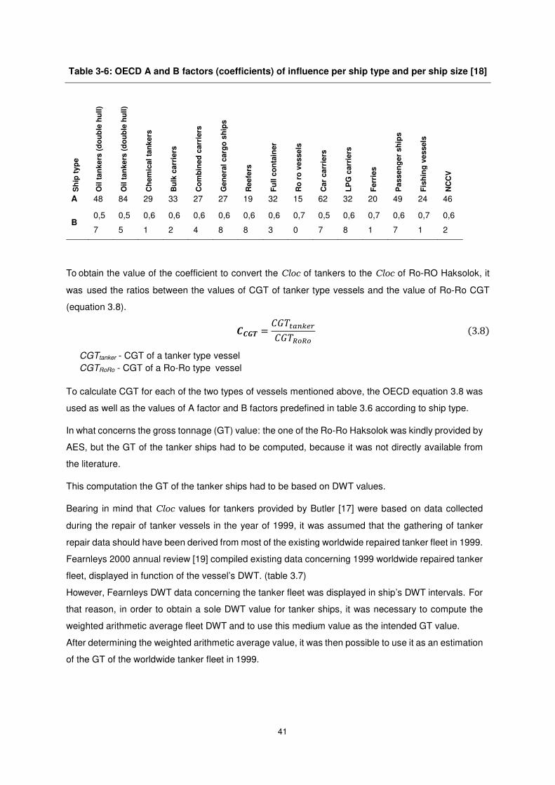
41

Table 3-6: OECD A and B factors (coefficients) of influence per ship type and per ship size [18]

To obtain the value of the coefficient to convert the Cloc of tankers to the Cloc of Ro-RO Haksolok, it

was used the ratios between the values of CGT of tanker type vessels and the value of Ro-Ro CGT

(equation 3.8).

88F� = &BC126G*�&BCH�H�

3.8�

CGTtanker - CGT of a tanker type vessel

CGTRoRo - CGT of a Ro-Ro type vessel

To calculate CGT for each of the two types of vessels mentioned above, the OECD equation 3.8 was

used as well as the values of A factor and B factors predefined in table 3.6 according to ship type.

In what concerns the gross tonnage (GT) value: the one of the Ro-Ro Haksolok was kindly provided by

AES, but the GT of the tanker ships had to be computed, because it was not directly available from

the literature.

This computation the GT of the tanker ships had to be based on DWT values.

Bearing in mind that Cloc values for tankers provided by Butler [17] were based on data collected

during the repair of tanker vessels in the year of 1999, it was assumed that the gathering of tanker

repair data should have been derived from most of the existing worldwide repaired tanker fleet in 1999.

Fearnleys 2000 annual review [19] compiled existing data concerning 1999 worldwide repaired tanker

fleet, displayed in function of the vessel’s DWT. (table 3.7)

However, Fearnleys DWT data concerning the tanker fleet was displayed in ship’s DWT intervals. For

that reason, in order to obtain a sole DWT value for tanker ships, it was necessary to compute the

weighted arithmetic average fleet DWT and to use this medium value as the intended GT value.

After determining the weighted arithmetic average value, it was then possible to use it as an estimation

of the GT of the worldwide tanker fleet in 1999.

Sh

ip t

yp

e

Oil t

an

kers

(d

ou

ble

hu

ll)

Oil t

an

kers

(d

ou

ble

hu

ll)

Ch

em

ical

tan

kers

Bu

lk c

arr

iers

Co

mb

ined

carr

iers

Gen

era

l carg

o s

hip

s

Reefe

rs

Fu

ll c

on

tain

er

Ro

ro

vessels

Car

carr

iers

LP

G c

arr

iers

Ferr

ies

Passen

ger

sh

ips

Fis

hin

g v

essels

NC

CV

A 48 84 29 33 27 27 19 32 15 62 32 20 49 24 46

B 0,5

7

0,5

5

0,6

1

0,6

2

0,6

4

0,6

8

0,6

8

0,6

3

0,7

0

0,5

7

0,6

8

0,7

1

0,6

7

0,7

1

0,6

2

42

Table 3-7: 1999 DWT shipped by the worldwide tanker fleet segmented by ship’s DWT

Vessel’s DWT intervals (1000 of tons)

10-25 25-40 40-50 50-80 80-120 120-200 200-320 320

Vessel’s DWT intervals average (1000 of tons)

17.5 32.5 45 65 100 160 260 320

Carried DWT (1000000 of tons)

6.3 19.7 12.3 18.4 49.3 41.6 103.4 21.7

Once this tanker GT value was calculated, the next step was to obtain the corresponding CGT value.

So as to, the marine traffic website was searched to identify a tanker with a DWT value near to the

tanker arithmetic average DWT in order to obtain a GT value that could be used as the intended tanker

CGT value. Once both the values of CGT for Ro-Ro Haksolok and for tankers ships were computed,

it was then possible to calculate the ratio between them, and to determine the value of the coefficient

to convert the Cloc of tankers to the Cloc of Ro-RO Haksolok. (results in table 3.9)

3.2.2.2.5 Calculation of traditional outfitting manufacturing Man-hours

Butler [17] states that the pipe section shape and pipe section length are factors that increase the

number of manufacturing Man-hours (Mhmanuf), and for that reason this had to be taken in consideration

for the Man-hours calculations.

The following equation was developed

��JKL�M = �ℎ$%N26�0 1 + &�� . �� + &��. �� 3.9�

MhND manuf - Unitary Mh straight pipe manufacturing from table 3.8

Ccu - Shape coefficient

ncu - Number of curves

Cbrch - Branches coefficient

nbrch - Number of branches

The number of Man-hours used in pipe fabrication depends linearly on the pipe length (table 3.8) but

also depends of ND and on the pipe shape (to calculate the manufacturing time increase due to shape,

the coefficients from 3.2.2.2 were used).

Table 3-8: Unitary straight pipe manufacturing Man-hours [20]

The values of Man-hours used in pipe repair (table 3.2) also depend on the size of pipe’s nominal

diameter.

An important point is the fact that the values of pipe manufacturing increase linearly alongside with pipe

length. Therefore, it can be said that dimension variation will affect the number of Man-hours.

ND (mm) Mh/m 32 0.11

65 0.13

80 0.13

150 0.17

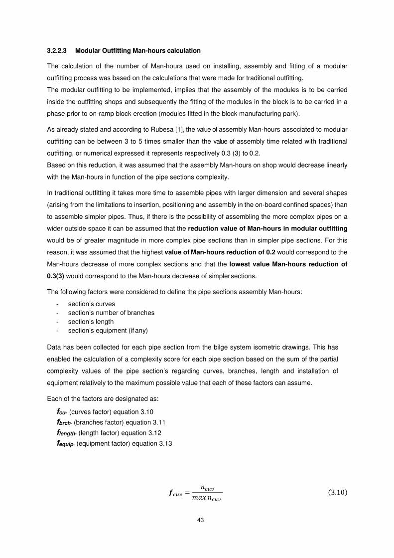
43

3.2.2.3 Modular Outfitting Man-hours calculation

The calculation of the number of Man-hours used on installing, assembly and fitting of a modular

outfitting process was based on the calculations that were made for traditional outfitting.

The modular outfitting to be implemented, implies that the assembly of the modules is to be carried

inside the outfitting shops and subsequently the fitting of the modules in the block is to be carried in a

phase prior to on-ramp block erection (modules fitted in the block manufacturing park).

As already stated and according to Rubesa [1], the value of assembly Man-hours associated to modular

outfitting can be between 3 to 5 times smaller than the value of assembly time related with traditional

outfitting, or numerical expressed it represents respectively 0.3 (3) to 0.2.

Based on this reduction, it was assumed that the assembly Man-hours on shop would decrease linearly

with the Man-hours in function of the pipe sections complexity.

In traditional outfitting it takes more time to assemble pipes with larger dimension and several shapes

(arising from the limitations to insertion, positioning and assembly in the on-board confined spaces) than

to assemble simpler pipes. Thus, if there is the possibility of assembling the more complex pipes on a

wider outside space it can be assumed that the reduction value of Man-hours in modular outfitting

would be of greater magnitude in more complex pipe sections than in simpler pipe sections. For this

reason, it was assumed that the highest value of Man-hours reduction of 0.2 would correspond to the

Man-hours decrease of more complex sections and that the lowest value Man-hours reduction of

0.3(3) would correspond to the Man-hours decrease of simpler sections.

The following factors were considered to define the pipe sections assembly Man-hours:

- section’s curves

- section’s number of branches

- section’s length

- section’s equipment (if any)

Data has been collected for each pipe section from the bilge system isometric drawings. This has

enabled the calculation of a complexity score for each pipe section based on the sum of the partial

complexity values of the pipe section’s regarding curves, branches, length and installation of

equipment relatively to the maximum possible value that each of these factors can assume.

Each of the factors are designated as:

fcu- (curves factor) equation 3.10

fbrch- (branches factor) equation 3.11

flength- (length factor) equation 3.12

fequip- (equipment factor) equation 3.13

M<�9 = ��PQR �� 3.10�

44

M:;<� = ��PQR �� 3.11�

M?LTU� = V� !"ℎPQR V� !"ℎ 3.12�

M�� = *+�,-PQR *+�,- 3.13�

ncu - number of section’s curves

nbrch - number of section’s branches

nlength - section’s length

nequip - number of section’s equipment

max ncuv maximum number curves of all pipe sections

max nbrch - maximum number branches of all pipe sections

max nlength - maximum length of all pipe sections

max nequip - number of section’s equipment

The value of the complexity score, designated as pipe section’s ”f” factor(f) score, is calculated as the

sum of the values of the four above mentioned factors, equation 3.14.

M = M<�9 + M:;<� + M?LTU� + M�� W. XY�

Once each pipe segment’s f was calculated, the corresponding Man-hours reduction rate RMh was

computed by linear interpolation, equation 3.15

Z�� = [N�\ + [N�] − [N�\_ − ^ . _ − ^ � 3.15�

In which:

- RM h1 and RM h2 are the value immediately above and below the section’s RM h value

- f2 and f1 are the value immediately above and below the section’s f value

Having calculated each pipe section’s man-hour reduction factor RMh, the pipe section’s modular

outfitting assembly Man-hours could be computed by equation 3.16.

�� = [N�. �ℎ)a 3.16� Once every pipe section’s modular outfitting Man-hours assembly value was calculated, a sum of all

section’s Man-hours was obtained in order to enable its comparison with the sum of the total traditional

outfitting pipe section’s assembly Man-hours, as per equation 3.17.

∆�� = � ℎ)a − � ℎNa 3.17�

45

3.3 Results and Analysis

As defined in section 3.2.1, the following three suitable bilge system zones for implementing modular

outfitting (table 3.1) and to analyze the Man-hours difference between the two outfitting methods

(traditional outfitting versus modular outfitting) were selected:

1. Engine Room (near engine room aft bulkhead)

2. Engine Room (near engine room fwd bulkhead)

3. Auxiliary Equipment Room 1

Before presenting the results concerning modular outfitting Man-hours assembly calculation it is

important to specify two intermediate calculation steps concerning CGT ratio (CCGT ) and concerning the

correspondence between the f value and reduction rate RMh.

The coefficient CCGT corresponds to the ratio between the Haksolok CGT and a tanker CGT. The tanker

CGT was computed from the GT of the tanker vessel ”Li Chi” with a DWT similar to the weighted arithmetic

average DWT value of the 1999 tanker fleet.

The Haksolok CGT was computed through equation 3.8 from its actual GT value.

Table 3.9 displays the CGT ratio parameters.

Table 3-9: CGT tanker and Ro-Ro values

Vessels DWT GT CGT RATIO* Tanker ”Li Chi” 48.653 30.325 - -

1999 Tanker Fleet weighted arithmetic average

47.914 30.000* 17.108 4,32

Ferry/Ro – Ro ”Haksolok” - 2.095 3.958

* estimated from the ”Li Chi” GT based on DWT similarity

As previously stated, the calculations of the reduction in Man-hours from traditional outfitting to modular

outfitting implementation were based on the correspondence between pipe section (f factor) and Man-

hours reduction rates defined on the literature [1].

f factor score was calculated for every pipe element, as per the above methodology, and then it was

possible to define the complexity score range which contained all the values, within a range in which the

maximum value corresponds to 3.1 and a minimum value to 0.

Considering that on the transition from traditional outfitting to modular outfitting, complex pipes assembly

time would lead to a greater improvement than simple pipe assembly times, it was empirically defined

that a section with f =3.1 would lead to a five times decrease [1] and that a section with f =0 would lead

a three times decrease [1]. This translates into a Mh reduction rate of 0.3(3) for the complexity value of

0 and a reduction rate of 0.2 to a complexity rate of 3.1 (table 3.10).

Table 3-10: MO versus TO - Man-hours (Mh) reduction

Complexity score (f) MO vs TO -

Mh reduction rate

0 0.3(3) 3.1 0.2

46

Then, using a trend line (linear interpolation), it was computed the Mh reduction factors for intermediate f

values. These intermediate values were then used in the calculations of the Man-hours difference

between traditional outfitting and modular outfitting assembly methods for each one the pipe sections.

Once these intermediate calculation steps were specified, the results concerning modular outfitting Man-

hours assembly were computed.

The pipe section’s assembly Man-hours values for both traditional outfitting and modular outfitting, for

every analyzed pipe sections, are displayed in annex A.1 and are represented in figures 3.4.and 3.5.

Specific colours of bars were used for each one of the outfitting methods results:

- blue bar - for traditional outfitting method

- red bar - for modular outfitting method

When comparing the difference in assembly Man-hours between traditional outfitting method and

modular outfitting method, and in line with the assumption of the Man-hours reduction according to pipe

section complexity, it was possible to observe that in general the more the pipe sections were complex,

the greater was the magnitude of Man-hours reduction.

The four most complex and the four simplest pipe sections are described in table 3.11.

Table 3.11 shows the values obtained from equation 3.17. The properties of the four most complex pipe

sections and four least complex pipe sections of the bilge system are displayed in table 3.11.

The order of magnitude of Man-hours difference, designated as “Difference”, calculated by equation

3.17 is displayed in the last column of the already mentioned table 3.11.

The results in this column clearly show that the four most complex pipe sections have a more significant

man-hours difference than the four simplest pipe sections, when comparing traditional outfitting and

modular outfitting.

Table 3-11: More complex and least complex Pipe sections description

WBS Yard code ND (mm)

Length

(m) Curves Branch Valves

Pumps&

Filters

TO

Total Mh

MO

Total Mh diff**

1.2.3.1* 041005 80 4.41 3 2 0 2 37.38 7.48 29.90 1.1.6.2* 031002 80 4.03 0 0 0 0 28.10 7.82 20.27 2.3.7.1* 105001 80 2.48 4 0 0 0 27.84 7.46 20.38 2.3.2.2* 041011 80 2.33 7 0 1 0 27.60 6.40 21.20

1.2.8.1* 009001 32 0.53 1 0 0 0 4.53 1.43 3.10

1.2.11.2* 003001 32 0.52 1 0 0 0 4.49 1.42 3.07

1.2.8.2* 009001 32 0.31 1 0 1 0 3.89 1.13 2.77

1.1.2.2* 013001 32 0.22 1 0 1 1 3.64 0.97 2.68 *More complex pipe sections; *Less complex pipe sections; ** Pipe section difference in Mh between TO and MO

The pipe section that spent the largest amount of Mh to be assembled, according to the defined work

breakdown structure, was section 2.8.1. This section took 37.38 Mh to be assembled by a traditional

outfitting method and 7.48 Mh to be assembled by a modular outfitting method, therefore, there is a

difference of 29.90 Mh.

Analyzing the simplest section to be fit, section 2.6.2, it is possible to verify that the different between

the outfitting methods is quite smaller, and that this difference equals 3.10 Mh.

47

Table 3.12 and figure 3.3 displays the results regarding the total difference between Man-hours used in

the traditional outfitting process and the used Man-hours in the modular outfitting (on-block) approach for

the selected parts of the bilge system computed according to equation 3.17. The raw values used in the

sum are displayed in table A.1 (Annex A).

In figure 3.3, trendlines were computed for both curves. It is possible to observe that the trendlines

functions of each curve do not intercept on the positive domain (^ d _, f^ R ∈ ℝi�.

One of the trendlines function characteristics that must be outlined is that both trendline functions

diverges when the abscissa approaches infinity. This means that if the amount of pipe sections to be

assembled and fitted increases, the difference between traditional outfitting trendline and modular

outfitting trendline will also increase.

Figure 3-3: Man-hours used for pipe assembly process by TO or MO

Table 3-12: Summed results of MO and TO assembly Mh

For the three selected sections of the bilge system it can be observed that by using a modular outfitting

approach, about 26% of the assembling man hours used in the traditional outfitting method will be spend,

which in numerical terms, represents a decrease 548.80 Mh (a reduction of 74% of the workload).

Outfitting (modular) in integrated construction implies a design workload increase when compared with

non-integrated shipbuilding processes. In this study the designing workload was not included in the

displayed results.

Module structure manufacturing and welding to the fitting birth was also not held account in the bilge

system modular outfitting work flow computations.

y = 12.471x + 27.194

R² = 0.9888

y = 3.3485x + 8.0907

R² = 0.988

0

100

200

300

400

500

600

700

800

900

0% 25% 50% 75% 100%

AS

SE

MB

LY M

AN

-HO

UR

S

PROCESS % COMPLETION

TO

MO

Total Results Mh Sum of Traditional on-board Outfitting 781.67 Sum Modular on-block outfitting 202.87

Difference between TO and MO 548.80

48

Although both these elements were not considered in modular outfitting workload assessment, it can be

assumed that due to the large difference between both outfitting methods, modular outfitting would still

represent a work flow decrease when compared to traditional outfitting.

This total difference of 548.80 Mh results from the analysis performed on the scope of this study that

concerns only of part of a single piping system (bilge system), although it can be applied to all the piping

systems and other outfitting systems.

A ferry vessel such as the “Haksolok” contains numerous piping systems that have more and heavier

pipe sections than the bilge system. Therefore, it possible to extrapolate that the difference of both

outfitting methods would increase.

Hence, it is valid to extrapolate that modular outfitting implementation could represent a significant

decrease on the vessel’s outfitting workflow.

Figure 3.5 shows an example of the module to be implemented in modular outfitting zone number 1.

Figures 3.6 show the location inside the ship where the modular outfitting zone 1 module is to be fitted.

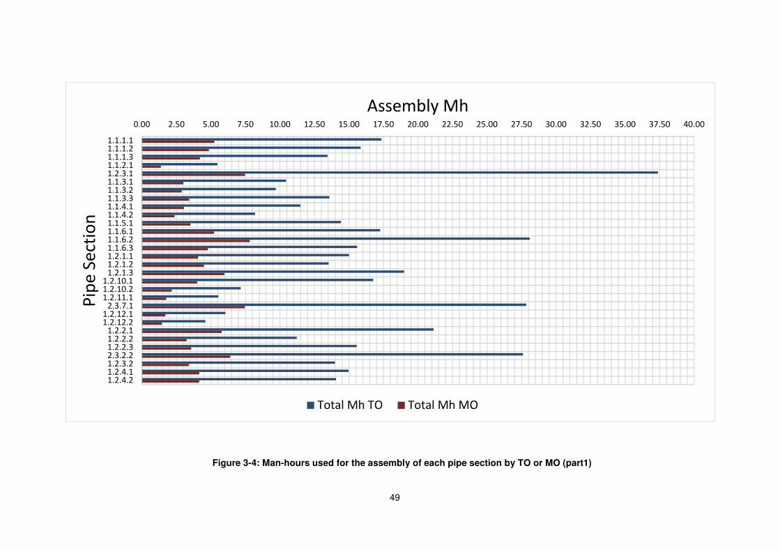
49

0.00 2.50 5.00 7.50 10.00 12.50 15.00 17.50 20.00 22.50 25.00 27.50 30.00 32.50 35.00 37.50 40.00

1.1.1.11.1.1.21.1.1.31.1.2.11.2.3.11.1.3.11.1.3.21.1.3.31.1.4.11.1.4.21.1.5.11.1.6.11.1.6.21.1.6.31.2.1.11.2.1.21.2.1.3

1.2.10.11.2.10.21.2.11.1

2.3.7.11.2.12.11.2.12.2

1.2.2.11.2.2.21.2.2.32.3.2.21.2.3.21.2.4.11.2.4.2

Assembly MhP

ipe

Se

ctio

n

Total Mh TO Total Mh MO

Figure 3-4: Man-hours used for the assembly of each pipe section by TO or MO (part1)

50

Figure 3.4: Man-hours used for the assembly of each pipe section by TO or MO (part 2)

0.00 2.50 5.00 7.50 10.00 12.50 15.00 17.50 20.00 22.50 25.00 27.50 30.00

1.2.5.11.2.5.21.2.6.11.2.6.21.2.7.11.2.7.21.2.8.1

1.2.11.21.2.8.31.2.9.11.2.9.22.3.1.12.3.2.11.2.8.22.3.2.32.3.3.12.3.3.22.3.4.12.3.6.12.3.4.22.3.6.22.3.5.11.1.2.22.3.7.22.3.8.12.3.8.22.3.9.12.3.9.2

2.3.10.12.3.10.2

Assembly MhP

ipe

Se

ctio

n

Total Mh TO Total Mh MO

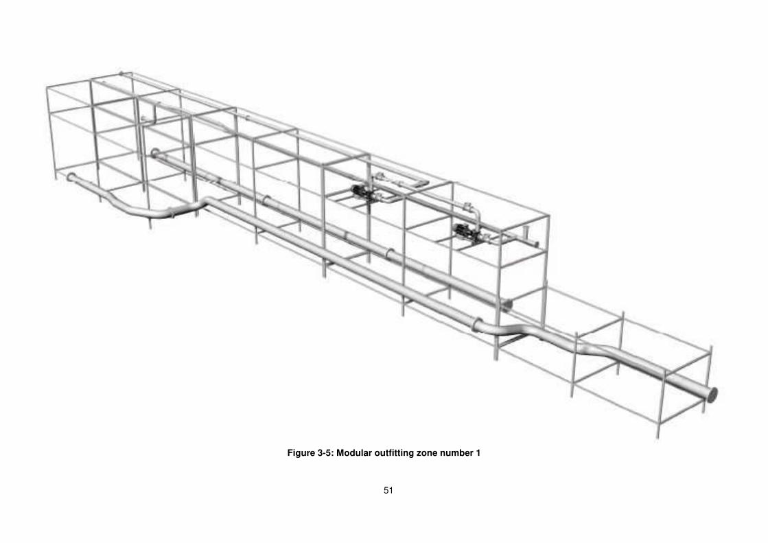
51

Figure 3-5: Modular outfitting zone number 1

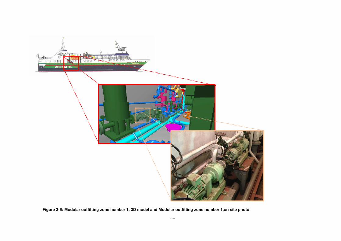
52

Figure 3-6: Modular outfitting zone number 1, 3D model and Modular outfitting zone number 1,on site photo

53

4

4 Systematic Layout Planning for

Modular Outfitting

Contents

4.1 Problem Modeling ......................................................................................................................................... 54

4.2 Methodology .................................................................................................................................. 54

4.3 Shipyard’s layout changes and results ........................................................................................................ 56

55

This chapter analyses the necessary changes in layout towards modular outfitting production

optimization. The main concern of this study was the location of the shops to be used for modular

outfitting assembly, in the existing shipyard (Atlantic Eagle Shipbuilding yard). Richard Muther’s

Systematic Layout Planning [12] was the chosen method to develop this analysis.

4.1 Problem Modeling

This Systematic Layout Planning analysis was made from a shipbuilding process perspective (instead

of ship repair process) using modular outfitting.

Considering the needs of modular outfitting units’ construction, it was assumed that a new dedicated

outfitting shop would be necessary. Therefore, three questions were formulated:

i. Where should the outfitting shop be located?

ii. What implications would it have on upgrading costs for the existing buildings/shops?

iii. What impact would it have on the flows of other shipyard’s processes?

Examining each question in detail and starting with the first question, the biggest problem was the

viability in terms of materials flow.

i. Due to its high cost, the constructing of a new building shop was out of the question therefore;

the implementation of a new outfitting shop should be on an existing facility. For the flow related

reasons, this new shop should be as close as possible to the block assembly park, however it

would important that the selected building would have the needed dimensions for the designated

activity.

ii. In what concerns the second question, there was a need to avoid significant added costs related

to building’s reworks.

iii. Regarding the third question, the following described constrains were identified. The first

constrain was that any change to the allocation of activities of the selected buildings should have a

minimal impact on the rest of the other processes in the shipyard. The second constrain was that

the shift of materials and equipment inherent the reallocation of function of the existing buildings,

should not add significant costs.

4.2 Methodology

The methodology implemented according to the process, represented in Figure 4.1 and described

below, was applied to answer the questions defined in section 4.1.

There are several methodologies for facility planning, namely: the Systematic Layout Planning

methodology (SLP), the Graph Based Theory (GBT), Dimensionless Block Diagram (DBD), among

others.

From this range of possible facility planning methodologies, SLP was selected, because of its perceived

advantages. SLP is an intuitive and easy learning technique with reliable results. Also, it has a vast

56

amount of available and thrust wordy information (articles, books and reports from real life facility

implantations). In what respects the CAD software Autocad, it exists an SLP related add-in (Proplanner)

which was very useful for the development of the layout analysis inherit to this dissertation.

In order to develop the layout study, it was necessary to collect data concerning paths of materials and

equipment and also concerning the average amount of time spent in each trip between buildings used in

traditional outfitting, so that the average time spent by the mobile equipment while transporting the loads

through the circuits defined for pipe assembly process could be estimated. (Figure 4.1).

Another piece of data that was crucial to this study was the technical layout drawing of the shipyard’s

scaled layout. The drawing of the AES shipyard layout that was supplied for the purpose of this study,

provided the information regarding the distances between shops and buildings.

Figure 4-1: Layout study process

After data collection, it was possible not only to project the layout changes that would optimize the

time and space efficiency of the modular outfitting implementation, but also to compare the traveling

times between the existing layout configurations with the modular outfitting suggested layout.

A specific flow software was used for the new layout design purpose (Flow Planner an AutoCAD add-

in) and this software provided two types of layout outputs:

i. First type concerns the Systematic Layout Planning Theory (mentioned in subsection 2.3.2)

and its two most important outputs were the Relationship Chart and the Space Relationship

Diagram, which are produced in the overall layout phase.

ii. Second type of output concerns the needed changes in the Material Flow Routes (distance

and time) resulting from the suggested modular outfitting adapted layout (see tables 4.5 and

4.4). It was necessary to produce sketches for both types of outputs.

The shipyard general arrangement layout drawing (for the existing traditional outfitting layout) provided

by AES did not include the previously defined Flow/Activity Diagrams or closeness relationship rates.

For this reason it was necessary to create this diagram and to define the relationship rates for both the

existing traditional outfitting layout and the new suggested modular outfitting layout. The traveling time

and the trip distances between shops outputs associated with the changes in routes were presented as

tables of results (tables 4.4 and 4.5). For both traditional outfitting and modular outfitting layouts, the

time and the distance between the routes of the shops/buildings, were calculated and subsequently

compared (tables 4.4 and 4.5).

57

4.3 Shipyard’s layout changes and results

4.3.1 Factor analysis

Following the theory stated in subsubsection 2.3.3.B, in order to comply with the readjusting layout

methods, it was necessary to breakdown the main layout readjusting problems.

When readjusting the layout to adapt it to the needs of the modular outfitting construction processes,

the matters in the three questions formulated in 4.1 had to be addressed, namely in what concerns: the

outfitting shop closeness to the block assembly, the park and the impact of activities reallocation on

building’s reworks costs and on material’s flows.

To implement the traditional outfitting layout and to simultaneously answer the three questions

formulated, the changes should be as follows:

i. Change no. 1 - Plasma cutting machine should be moved to a new location near the steel shop

ii. Change no. 2 - New outfitting shop should be placed into contiguous: to where the plasma

cutting machine used to be and the other where the old outfitting shop was

iii. Change no. 3 - Park to storage plates and steel profiles should be created near the plasma-

cutting machine

The suggested changes were based on the following rationales:

i. Change no. 1 aimed to decrease the distance between the cutting and steel shop and therefore,

to have a positive influence on the block manufacturing efficiency

ii. Change no. 2 was due to the fact that the place where the cutting machine used to be, was the

one that better fit in terms of flow analysis for the new outfitting shop, because this shop is closer

to the path that goes to the block assembly park

iii. Change no.3 is due to the fact that change 1 has relocated the cutting machine near the steel

shop that is further away from the reception park. There is a wide space near the new location of

the cutting machine that could be reorganized to accommodate a closer steel storage park

without significantly harming other production processes

As there were no available preexisting buildings near the steel shop area, change no. 1 would imply

the need for an extra building. In order to avoid high expenses, this building should be a pre-

fabricated building that could be either acquired or rented. The alternative of a pre-fabricated building

would potential reduce the costs of change no. 1, comparatively to the construction of a new building.

58

4.3.2 Layout changes - Advantages versus Disadvantages

Following the procedures mentioned in 2.3.3, the advantages and disadvantages of the layout changes

were weighed and rated.

For change no 1 (plasma cutting machine) and change no 2 (new outfitting shop), the advantages and

disadvantages were listed and rated in accordance to the code exposed in table 2.2 and the results

were compiled in tables 4.1, 4.2.

Table 4-1: Advantages vs disadvantages analysis for the changing of the cutting machine

position Cutting machine position

Existing Layout Suggested Layout Item Rating Item Rating

AD

VA

NT

AG

E 1 Shop with larger dimensions O 1 Closer to the steel shop A

2 More space to store and organize the pieces and plates to be cut

I 2 Closer to the prefabrication shop A

3 Closer to yard repair ramp E 3 Closer to block assembly park E

DIS

AD

VA

NT

AG

E

1 Further away from steel shop A 1 Further away from ship repair ramp E

2 Further away from pre-fabrication shop

A 2 Additional cost due to the need of a new building

A

3 Further away from block manufacturing park

E 3 Adds costs for moving the shop’s equipment towards the new location

I

Table 4-2: Advantages vs disadvantages analysis of the new outfitting shop

New Outfitting Shop

Existing Layout Suggested Layout

Item Rating Item Rating

AD

VA

NT

AG

E

1 Does not add costs of moving the shop’s equipment towards the new location

I 1 More space to assemble piping units A

2 2 Creates a hub point to all piping related processes

A

DIS

AD

VA

NT

AG

E

1

Does not have enough space for assembling modular outfitting units in a single shop

A 1 Adds costs for moving the shop’s equipment towards the new location

I

For the change no 3 (steel storage park relocation) no disadvantages were identified and so there was

no need to weighed against advantages. The two advantages identified were:

- Closeness of the steel storage park to the new location of the cutting machine reduces the

traveling time

- No dislodgement of any activity or equipment because the park reloction was in an empty area

and so no added costs are expected.

59

To numerically weigh the advantages against the disadvantages, the numerical factors associated with

the letter rating [12] were used. The numerical factors were within a range of zero to four, where zero is

represented by the letter ”U” and four by the letter ”A”.

Summing the numerical factor of each advantages/disadvantage (equation 4.1) the final weighed results

of the advocated layout changes were obtained and exposed on table 4.3.

j�T�Uk4l9m4no = p [Q"f !,6

,�` − p [Q"f !q

6

q�` 4.1�

Table 4-3: MO/TO advantages against disadvantages weigh

Advantages (i) Disadvantages (j) Difference (Eq. 4.1)

Cutting Machine Position

Suggested Layout 11 9 2

Existing Layout 6 11 -5

Wider Outfitting Shops

Suggested Layout 8 2 6

Existing Layout 2 4 -2

The major advantages of the existing traditional outfitting layout are:

- Existence of a large workshop for steel cutting processes

- Location of the steel cutting workshop nearby the repair ramp

The major disadvantages of the existing traditional outfitting layout are:

- Location of the cutting machine far away from steel shop location

- Location of the cutting machine far away from panel line shop location

- Location of the cutting machine far away from block manufacturing park location

The major advantages of the suggested modular outfitting layout are:

- Location of cutting machine nearby steel shop, panel line and block manufacturing park

- Existence of larger outfitting workshops

- Existence of a hub point for all outfitting related processes

- Closeness of the steel storage park to the new location of the cutting machine

The major disadvantages of the suggested modular outfitting layout are:

- Cutting machine further away from repair ramp

- Existence of added costs due to the renting/acquiring of a pre-fabricated building.

In terms of result discussion, the already existing traditional outfitting layout, had an overall non-

positive result when compared with the new suggested layout. This previous layout, as mentioned in

table 4.2, has some disadvantages that were associated with the order of magnitude of the distance

between the location of the cutting machine and the location of the steel shop and panel line.

Focusing now on the outfitting shops, the major disadvantages of the existing traditional outfitting

layout are related to the potential lack of space for the implementation of modular units assembly

processes. On the other hand, this layout has the advantage of being located nearby the ship repair

ramp.

Regarding the new suggested modular outfitting layout, the overall results were positive (table 4.3).

For all the proposed changes, most of the disadvantages are linked with the costs of equipment

60

repositioning process and of infrastructure.

As advocated before, the transference of the cutting machine towards a new location, would imply the

acquisition or the renting of a pre-fabricated building (because building of a new infrastructure would be

over costly).

The equipment repositioning process also has some associated costs but those, when compared with

the acquisition of a new infrastructure, have a smaller impact. The new suggested layout has various

advantages.

Moving the cutting machine into the new location would reduce the transportation time of the cut steel

plates towards the steel shop, the panel line and the block manufacturing park.

The increase of the available space for outfitting related activities due to the creation of a new outfitting

shop, it will also enable the suitable conditions for the implementation of more space demanding

activities, as it is the case of the assembly of piping segments in modular units.

This space increment will also result in the reinforcement of the piping hub role of that shipyard’s area.

Concentrating all the piping activity on this area will create a logistic center that can supply all the

construction needs both in ramps and piers.

4.3.3 Cost Comparison

Cost comparison was expressed in differences in traveling time between workstations. Following the

logic defined by Muther [12] and mentioned in subsection 2.3.3.3, there are three types of fields on which

cost comparison is made upon.

- Flow Index

- Transport Work

- Definitive material handling cost

The cost comparison study started by analyzing the existing traditional outfitting layout in order to define

a reference/control layout. The results obtained from this analysis provided the baseline values for the

comparison with the new suggested modular outfitting layout.

Those results were exported from the software Proplanner and were used, both for flow index and

transport work calculations.

The estimation of the definitive material handling costs would imply a more detailed analysis, that would

require a high level of expertise, concerning the position and the working rate of several units inside the

shops and the material handling methods (for plates, pipes, stiffeners, small sized equipment, large sized

equipment, and other equipment and materials). Therefore, it was considered out of the scope of this

master’s thesis.

Flow index was defined upon the theoretical procedures mentioned on subsection 2.3.2.

Two types of flow index outputs were obtained:

i. The Relationship Chart

ii. The Space Relationship Diagram

61

These outputs were generated for both the existing traditional outfitting layout and the suggested

modular outfitting layout.

Starting by the existing traditional outfitting layout, it has been stated that every piece of material and

equipment arrives in the reception park; thus, this park has type “A” relationship rates with several

shops and construction sites (construction ramp and pier).

The shops and the facilities (construction ramp, block manufacturing park, steel shop, panel line and

cutting shop) where the block manufacturing process is performed also have type “A” and “E”

relationship rates among them.

Regarding piping systems, currently the pipes are outsourced and manufactured outside the

shipyard. Hence in the shipyard they are merely assembled and tested on board. Additionally, if they

have some type of damage in terms of surface treatment, they might also be blasted and painted inside

the shipyard. Consequently, most of the pipe related flow in the shipyard occurs between the

reception park and the construction sites.

By observing table 4.2 a broader insight regarding the existing layout relation rates can be obtained.

A Space Relationship Diagram for traditional outfitting existing layout was created, using the data from

the Relationship Chart (figure 4.2), as represented by figure 1 of annex B. To avoid the diagram lines

overload only “A” type relations were drawn.

Several changes of the suggested new layout were advocated as mentioned in 4.3.1. Having created

a new shop and having redefined activities flow, logically, new relationship rates had to be delineated,

then, a new relationship chart was created.

Several relation rates can be highlighted in this new relationship chart (figure 4.3). First, the detach of

a new outfitting shop that due to its new functions is now the construction sites pipes supplier. Hence

this shop has kept an “A” type relation rate with the block manufacturing park and with the

construction ramp.

Figure 4-2: Existing TO layout relationship chart

RECEPTION PARK

CUTTING FACILITY

OUTFITTING SHOP

PIPE SHOP



CARPENTER SHOP

PANEL LINE

STEEL SHOP


PIER

CONSTRUCTION RAMP

35

31

30

29

28

27

17

11

10

4

3

1

VO WEL

LETT ER

A

E

I

O

U

CLO SENE SS RATI NG

ABSO LU TELY

NE CES SARY

ESPECI ALLY

IM PORTANT

IM PORTANT

O RD INA RY

UN IM PORTANT

COL OR

COD E

A

E

I

O

U

U

U

E

A

O

U

U

E

U

E

A

A

E

I

O

U

A

E

I

O

U

A

I O

U

A

E

I

OU

A

E

O

U

A

E

O

U

UU

U

U

U

E

E

EAA

AU U

U

U

A

OO

O

O

OO

O

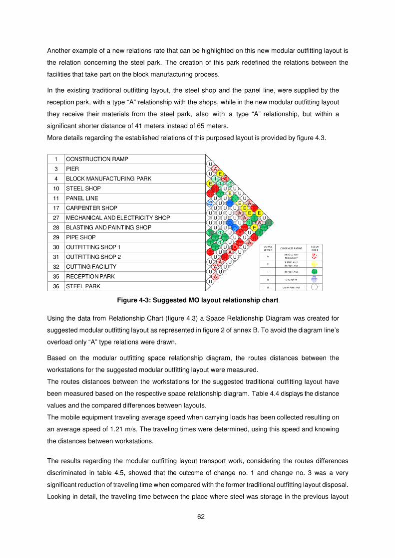
62

Another example of a new relations rate that can be highlighted on this new modular outfitting layout is

the relation concerning the steel park. The creation of this park redefined the relations between the

facilities that take part on the block manufacturing process.

In the existing traditional outfitting layout, the steel shop and the panel line, were supplied by the

reception park, with a type “A” relationship with the shops, while in the new modular outfitting layout

they receive their materials from the steel park, also with a type “A” relationship, but within a

significant shorter distance of 41 meters instead of 65 meters.

More details regarding the established relations of this purposed layout is provided by figure 4.3.

Figure 4-3: Suggested MO layout relationship chart

Using the data from Relationship Chart (figure 4.3) a Space Relationship Diagram was created for

suggested modular outfitting layout as represented in figure 2 of annex B. To avoid the diagram line’s

overload only “A” type relations were drawn.

Based on the modular outfitting space relationship diagram, the routes distances between the

workstations for the suggested modular outfitting layout were measured.

The routes distances between the workstations for the suggested traditional outfitting layout have

been measured based on the respective space relationship diagram. Table 4.4 displays the distance

values and the compared differences between layouts.

The mobile equipment traveling average speed when carrying loads has been collected resulting on

an average speed of 1.21 m/s. The traveling times were determined, using this speed and knowing

the distances between workstations.

The results regarding the modular outfitting layout transport work, considering the routes differences

discriminated in table 4.5, showed that the outcome of change no. 1 and change no. 3 was a very

significant reduction of traveling time when compared with the former traditional outfitting layout disposal.

Looking in detail, the traveling time between the place where steel was storage in the previous layout

STEEL PARK

RECEPTION PARK

CUTTING FACILITY

OUTFITTING SHOP 2

OUTFITTING SHOP 1

PIPE SHOP



CARPENTER SHOP

PANEL LINE

STEEL SHOP


PIER

CONSTRUCTION RAMP

AA

A

U

A

E

U

O

I

I

U

U

U

U

U

A

A

A

A

A

A

AA

36

35

32

31

30

29

28

27

17

11

10

4

3

1

VO WE L

LETT ER

A

E

I

O

U

CLO SENESS RATI NG

ABSO LU TE LY

NECES SARY

E SPECI ALLY

IM PORTANT

IM PORTANT

O RD INA RY

UN IM PORTANT

COL OR

COD E

I

U

O

I

O

I

II

II

II

I

II

I

II

U

U

U

U

UU

UU

U

U

A

A

A

A

AA

A

A

AO

E

E

E

E

EE

E

U

UU

U

U

UU

U

U

U

U

U

U

U

U

UU

U U

UU

UU

U

63

and the place where it would be storage in the suggested modular outfitting layout (near to the new

cutting machine location), decreased by 37%. The traveling between the cutting machine and the steel

shop had a remarkable decrease of 75%.

Cutting machine position 1 Cutting machine position 2

From To Trip

Distance (m) To

Trip

Distance (m)

Cu

ttin

g

ma

ch

ine

Pre- fabrication 111.7 Pre- fabrication 38.12

Receiving park (P1) 65.25 Steel storage park 41.05

Steel shop 118.83 Steel shop 29.22

Construction ramp 127.34 Construction ramp 105.61

Table 4-5: Traveling times between workstations

Cutting machine position 1 Cutting machine position 2

From To Travel Time (s)

To Travel Time (s)

Relative Difference

Cu

ttin

g

ma

ch

ine

Pre- fabrication 93.08 Pre- fabrication 31.77 66%

Receiving park (P1) 54.38 Steel storage park 34.21 37%

Steel shop 99.02 Steel shop 24.35 75%

Construction ramp 106.11 Construction ramp 88.01 17%

Figure 4.4 and 4.5 display the flow charts of the process to be implemented in the suggested layout.

The changes between the existing and suggested layout would allow a smooth implementation of both,

the module structure manufacturing and assembly process (figure 4.5) and the module assembly

process (4.4).

In the case of the module structure manufacturing, the work flow gain margin from the repositioning of

the cutting machine would depend of the number of parts and pieces to be cut, however, it is secure to

state that it would be positive, when compared with the existing layout.

In the case of the module assembly process it is not possible to perform a gain margin comparison

between existing and suggested layout because it is a new process that was not contemplated in the

existing layout.

Table 4-4: Trip distances between workstations

64

Figure 4-4: Suggested MO module assembly flow chart

Figure 4-5: Suggested MO module structure assembly flow chart

Time (s)DESCRIPTION Distance

SYMBOL

FLOW PROCESS CHART

-Storage in Receiving Park -

54,38Storage in Receiving Park 65,25








StorageInspectionDelayTransportOperation

MODULE ASSEMBLY

Time (s)DESCRIPTION Distance

SYMBOL

FLOW PROCESS CHART










StorageInspectionDelayTransportOperation

MODULE ASSEMBLY

65

5

5 Modular Outfitting Implementation

Risk Management

Contents

5.1 Scope of the problem .................................................................................................................................... 66

5.2 Methodology ............................................................................................................................................... 66

5.3 Results Analysis ............................................................................................................................................ 70

67

This chapter describes a Risk Management procedure that was undertaken to assess the implementation

of modular outfitting construction approach.

It addresses in particularly the processes of: Risk Identification, Qualitative Analysis and Risk Response

and Critical Success Factors.

Critical Success Factors, CSFs for this outfitting practice are also described in detail, because they are

decisive and crucial to obtain positive results, in order to achieve the established objectives and to

achieve success.

5.1 Scope of the problem

The definition of risk and the need to measure risk before initiating any kind of action was developed

in section 2.4.

Thus, like in any project, when implementing a new type of production technique or approach in a

shipbuilding process it is necessary to identify, assess and manage the risks of the new project.

Therefore, the following three questions are addressed in this chapter:

- What are the existing risks of Modular Outfitting Approach?

- What is the likelihood and impact of those risks?

- How to operate to respond to that risk?

5.2 Methodology

To answer the questions formulated in the previous sections, it was necessary to identify the risks, to

perform a qualitative analysis and to develop a risk response table. These analytic tools are part of the

risk management procedure (see section 2.4).

5.2.1 Risk Identification

The first step taken was the risk identification. Modular Outfitting approach is composed by seven different

processes and each one has specific risks that result from specific causes.

1. Design

2. Module parts manufacturing

3. Module assembly

4. Dimensional control and running tests in shop

5. Module transportation and fitting on-block

6. Block assembly, fitting and installing

7. Final trials

Figure 5.1 graphically shows the workflow of Modular Outfitting including the sequence decision points.

68

Figure 5-1: Modular outfitting workflow

START

DESIGN

END

DESINGN DRAWINGS APPROVAL

NOYES

MODULE PARTS MANUFACTURING

MODULE ASSEMBLY

DIMENSIONAL CONTROL AND RUNNING

TESTS

MODULE TRANSPORTATION AND

FITTING ON BLOCK

ON BLOCK ASSEMBLING

FINAL TRIALS

NOYES

NOYES

PIPE MANUFACTURING

MODULE SUPPORT

MANUFACTURING

MODULE ISOMETRIC TESTING

HYDRAULIC TESTS

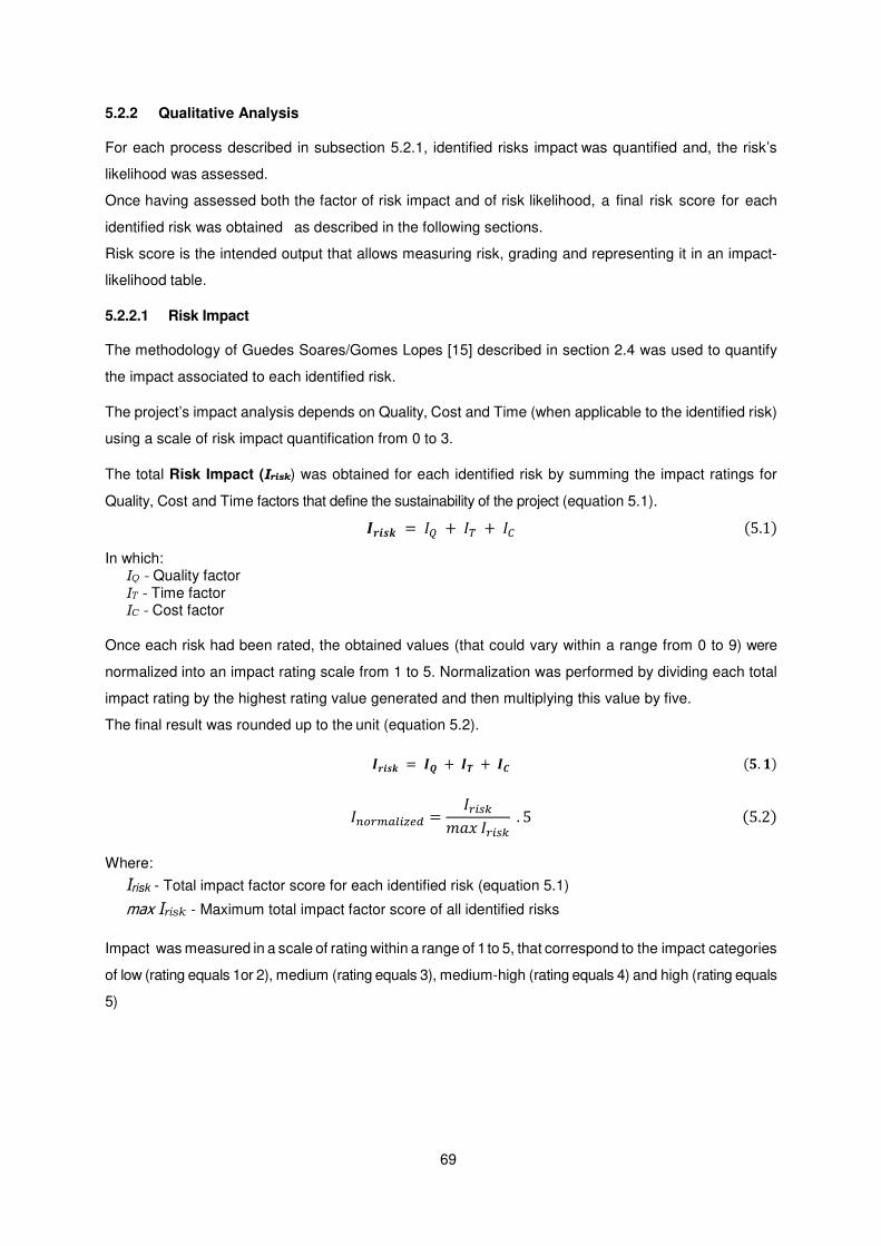
69

5.2.2 Qualitative Analysis

For each process described in subsection 5.2.1, identified risks impact was quantified and, the risk’s

likelihood was assessed.

Once having assessed both the factor of risk impact and of risk likelihood, a final risk score for each

identified risk was obtained as described in the following sections.

Risk score is the intended output that allows measuring risk, grading and representing it in an impact-

likelihood table.

5.2.2.1 Risk Impact

The methodology of Guedes Soares/Gomes Lopes [15] described in section 2.4 was used to quantify

the impact associated to each identified risk.

The project’s impact analysis depends on Quality, Cost and Time (when applicable to the identified risk)

using a scale of risk impact quantification from 0 to 3.

The total Risk Impact (Irisk) was obtained for each identified risk by summing the impact ratings for

Quality, Cost and Time factors that define the sustainability of the project (equation 5.1).

r;�ms = tu + t) + t' 5.1�

In which: IQ - Quality factor IT - Time factor IC - Cost factor

Once each risk had been rated, the obtained values (that could vary within a range from 0 to 9) were

normalized into an impact rating scale from 1 to 5. Normalization was performed by dividing each total

impact rating by the highest rating value generated and then multiplying this value by five.

The final result was rounded up to the unit (equation 5.2).

r;�ms = rv + r� + r8 w. X�

t6��.2�,x*y = t�,/GPQR t�,/G

. 5 5.2�

Where:

Irisk - Total impact factor score for each identified risk (equation 5.1)

max Irisk - Maximum total impact factor score of all identified risks

Impact was measured in a scale of rating within a range of 1 to 5, that correspond to the impact categories

of low (rating equals 1or 2), medium (rating equals 3), medium-high (rating equals 4) and high (rating equals

5)

70

5.2.2.2 Risk Likelihood

The other input of the qualitative analysis is the likelihood of risk occurrence. Like in the risk impact,

likelihood was expressed in a scale of likelihood scores within a range of 1 to 5, that correspond to the

likelihood categories of low (rating between 1-2), medium (rating equals 3), medium-high (rating equals 4)

and high (rating equals 5). The likelihood of occurrence of each identified risk was empirically estimated.

5.2.2.3 Risk Assessment in function of risk Impact and Likelihood

The risk assessment was based on the impact-likelihood risk score results, computed by equation 5.3.

[fz{|}~�� = �f{�Vfℎ~~� . tP�Q}" 5.3�

The likelihood-impact tables developed in the qualitative analysis of this dissertation’s was based in

PMBOOK qualitative risk assessment approach [14], although adapted.

In the PMBOOK approach [14], the likelihood rating range is between 0 and 1 points and the and impact

rating range is between 0 and 0.1 points (table 5.1). The resulting impact-likelihood scores are classified

and highlighted in a scale of color. In this scale the highest risk scores are represented by a red color,

the lowest risk scores are represented by a green color, and the remaining risk score results are

represented by intermediate colors that show the magnitude of the score by a color degrade.

Table 5-1: Example of a PMBOOK Impact-Likelihood table [14]

In this dissertation’s, the likelihood rating range is between 1 and 5 points, which has a linear relation

with the mentioned PMBOK rating range of 0 to 1 point.

Same procedure was applied to the impact scale. In the PMBOK approach, the impact range is between

0 and 0.1 point, but in this dissertation’s impact range is between 1 and 5 points, which once again is a

linear function of the PMBOOK impact scale.

This increase of the scale points from 1 to 5 aimed to improve the ability to identify in detail the relative

differences between the values of risk impact and of risk likelihood.

For each of these two dimensions of risk assessment, the rating values were categorized in low (rating

equals 1); medium (rating between 2-4) and high (rating equals 5). No color scale was adopted for the

Impact-Likelihood scores.

The range of values of risk score computed according to equation 5.3 is from 1 to 25 points.

On section 5.3 the identified risk will be exposed with their risk score and proposed risk response.

0.9

0.7

0.5

0.3

0.1

0.03 - 0.040.05 - 0.070.08 - 0.10.12 - 0.14

0.005

0.05 0.1

0.05

0.04

0.03

0.02

0.09

0.07

0.05

0.03

0.01

0.36

0.28

0.2

0.12

0.04

0.18

0.14

0.1

0.06

0.2

LIK

EL

IHO

OD

* Over an objective Ex: Cost, Time, Scope, Quality

0.02

Color code

IMPACT *

Low Magnitude Hi gh Magni tudeMedium

Magni tude

0.4

0.72

0.56

0.4

0.24

0.08

0.8

0.005

0.01 - 0.02

0.18 - 0.36

0.56 - 0.72

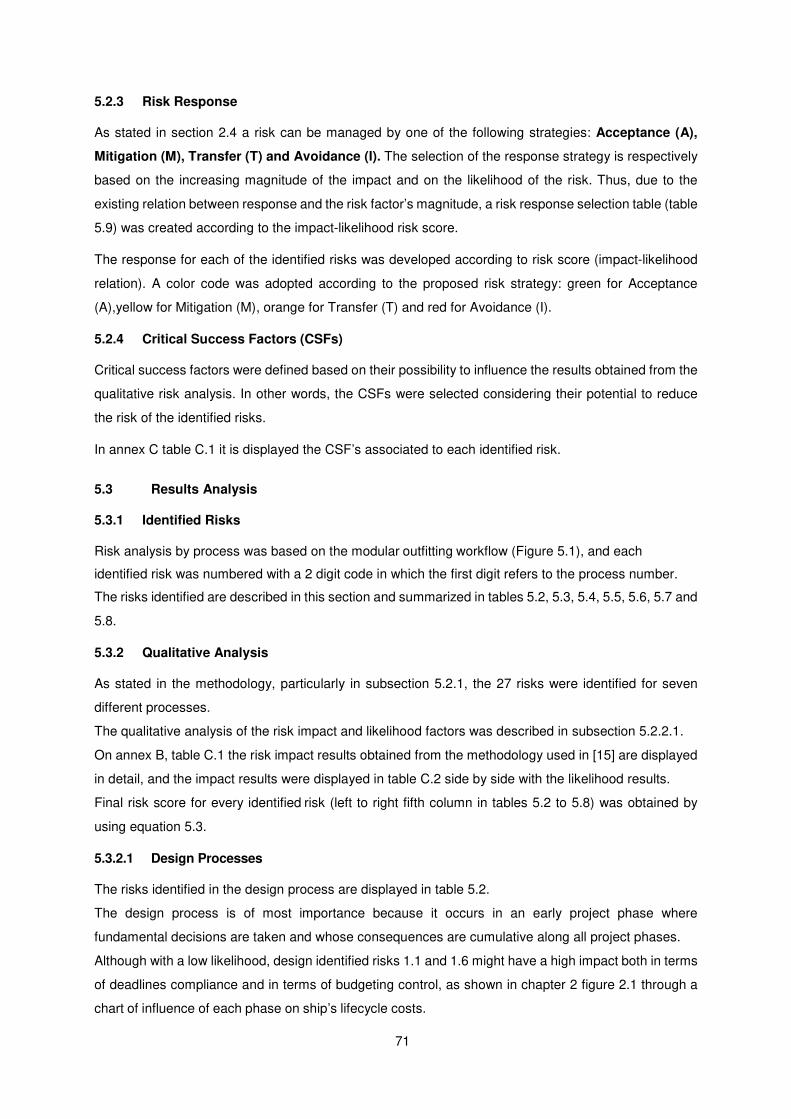
71

5.2.3 Risk Response

As stated in section 2.4 a risk can be managed by one of the following strategies: Acceptance (A),

Mitigation (M), Transfer (T) and Avoidance (I). The selection of the response strategy is respectively

based on the increasing magnitude of the impact and on the likelihood of the risk. Thus, due to the

existing relation between response and the risk factor’s magnitude, a risk response selection table (table

5.9) was created according to the impact-likelihood risk score.

The response for each of the identified risks was developed according to risk score (impact-likelihood

relation). A color code was adopted according to the proposed risk strategy: green for Acceptance

(A),yellow for Mitigation (M), orange for Transfer (T) and red for Avoidance (I).

5.2.4 Critical Success Factors (CSFs)

Critical success factors were defined based on their possibility to influence the results obtained from the

qualitative risk analysis. In other words, the CSFs were selected considering their potential to reduce

the risk of the identified risks.

In annex C table C.1 it is displayed the CSF’s associated to each identified risk.

5.3 Results Analysis

5.3.1 Identified Risks

Risk analysis by process was based on the modular outfitting workflow (Figure 5.1), and each

identified risk was numbered with a 2 digit code in which the first digit refers to the process number.

The risks identified are described in this section and summarized in tables 5.2, 5.3, 5.4, 5.5, 5.6, 5.7 and

5.8.

5.3.2 Qualitative Analysis

As stated in the methodology, particularly in subsection 5.2.1, the 27 risks were identified for seven

different processes.

The qualitative analysis of the risk impact and likelihood factors was described in subsection 5.2.2.1.

On annex B, table C.1 the risk impact results obtained from the methodology used in [15] are displayed

in detail, and the impact results were displayed in table C.2 side by side with the likelihood results.

Final risk score for every identified risk (left to right fifth column in tables 5.2 to 5.8) was obtained by

using equation 5.3.

5.3.2.1 Design Processes

The risks identified in the design process are displayed in table 5.2.

The design process is of most importance because it occurs in an early project phase where

fundamental decisions are taken and whose consequences are cumulative along all project phases.

Although with a low likelihood, design identified risks 1.1 and 1.6 might have a high impact both in terms

of deadlines compliance and in terms of budgeting control, as shown in chapter 2 figure 2.1 through a

chart of influence of each phase on ship’s lifecycle costs.

72

Table 5-2: Design Process Identified Risks

Likelihood Impact Risk Factor

Risk Response

1 DESIGN

1.1 Poor identification of equipment and

outfitting components forming in modular block 2 5 10 M

1.2 Lack of preliminary and further studies

in outfitting modular implementation strategy 4 4 16 M

1.3 Unexperienced designers on conceptual production manufacturing

2 3 6 M

1.4 New procedures and techniques 2 1 2 A

1.5 Inadequate working plans, production and detail drawings

4 5 20 T

1.6 Inadequate inspection and control methodology 1 5 5 M

Poor identification (or design) of equipment and outfitting components forming in a modular block (risk

1.1) could imply, not only delays but also additional costs related to rework during the construction

phase.

Inspection and control step is a well-established risk, so it has low likelihood of not being adequate to

verify compliance with the requirements, but in case of not being able to scope errors, it is prone to have

a high impact.

In what concerns inadequate working plans, production and detail drawings (risk 1.5), there is a medium

likelihood of not being possible, at a very early phase, to anticipate with accuracy every practical

requirement. Flaws in design process have a high impact in all subsequent modular outfitting processes

5.3.2.2 Module Parts Manufactured Process

The process of the manufacturing of module parts (as well as the process of module assembly) is mostly

susceptible to risks related with quality control and with schedule compliance by the supplier-

s/outsourced entities.

.In what concerns quality control, the risks are the existence of elements out of form, out of dimensions,

and with welding faults. The high impact of these risks results from the probability of identification of faulty

parts on advanced phases of assembly, or from the possible delays resulting from the need of reordering

the defective parts. Although having a high impact risk, they have a low likelihood due to the certified

compliance of the product manufacturing entities (shipyard pipe suppliers) with the quality standards.

The identified risks of Module Parts Manufactured are displayed in table 5.3.

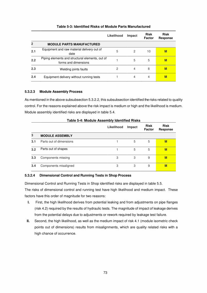
73

Table 5-3: Identified Risks of Module Parts Manufactured

5.3.2.3 Module Assembly Process

As mentioned in the above subsubsection 5.3.2.2, this subsubsection identified the risks related to quality

control. For the reasons explained above the risk impact is medium or high and the likelihood is medium.

Module assembly identified risks are displayed in table 5.4.

Table 5-4: Module Assembly Identified Risks


Risk Response

3 MODULE ASSEMBLY

3.1 Parts out of dimensions 1 5 5 M

3.2 Parts out of shapes 1 5 5 M

3.3 Components missing 3 3 9 M

3.4 Components misaligned 3 3 9 M

5.3.2.4 Dimensional Control and Running Tests in Shop Process

Dimensional Control and Running Tests in Shop identified risks are displayed in table 5.5.

The risks of dimensional control and running test have high likelihood and medium impact. These

factors have this order of magnitude for two reasons:

I. First, the high likelihood derives from potential leaking and from adjustments on pipe flanges

(risk 4.2) required by the results of hydraulic tests. The magnitude of impact of leakage derives

from the potential delays due to adjustments or rework required by leakage test failure.

II. Second, the high likelihood, as well as the medium impact of risk 4.1 (module isometric check

points out of dimensions) results from misalignments, which are quality related risks with a

high chance of occurrence.

Likelihood Impact Risk

Factor Risk

Response

2 MODULE PARTS MANUFACTURED

2.1 Equipment and raw material delivery out of

date 5 2 10 M

2.2 Piping elements and structural elements, out of

forms and dimensions 1 5 5 M

2.3 Welding joints faults 2 4 8 M

2.4 Equipment delivery without running tests 1 4 4 M

74

Table 5-5: Dimensional Control and Running Tests in Shop Identified Risks

Likelihood Impact Risk

Factor Risk

Response

4 DIMENSIONAL CONTROL AND RUNNING TESTS IN SHOP

4.1

Module isometric check points out of tolerance in the three-dimensional measurement

5 3 15 M

4.2 Hydraulic tests failure due to leakages 4 4 16 M

5.3.2.5 Transportation and Fitting On-Block Process

The risks of module transportation and fitting on-block process concern two different procedures:

the hoisting related procedures (risks 5.1, 5.2 and 5.3) and the fitting procedures (risks 5.4, 5.5 and

5.6).

In hoisting, the risks are associated to noncompliance with the operating safety rules and to

noncompliance with the material safety rules. Employee’s vehicle and crane handling certification

along with the regular update of the certificated licenses are critical practices regarding risk increase

avoidance.

Fitting procedures are the ones that have the highest risk score, both in terms of impact and of

likelihood.

The procedure of most importance in modular outfitting approach is the correct scheduling between two

parts of integrated construction (risk 5.5): the block manufacturing (part of the hull block construction

method) and the module assembly (part of zone outfitting method).

Defective coordination between the two mentioned parts of integrated construction could result in severe

delays and added costs, by holding other process parts. An example of a critical situation would be

holding the start of a new block assembly process due to delays in the outfitting modules that were to

be fitted on a previous block (that would remain for a longer time in the construction park).

Besides scheduling risks, on block fitting procedures has other risks such as potential interferences with

other equipment/structures as a result of misalignment of boundary spaces and also as the existence of

damaged parts (which implies removing, manufacturing and re-assemble that same part).

Both these identified risks have high likelihood and medium impact, due to the probable need of rework

triggered either by the misalignment correction or by damage component substitution.

Transportation and Fitting On-Block identified risks are displayed in table 5.6.

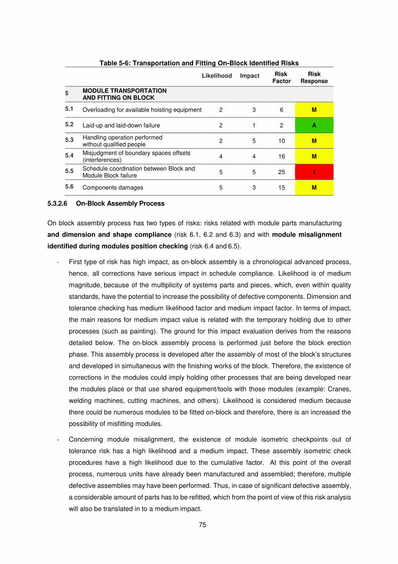
75

Table 5-6: Transportation and Fitting On-Block Identified Risks


Risk Response

5 MODULE TRANSPORTATION AND FITTING ON BLOCK

5.1 Overloading for available hoisting equipment 2 3 6 M

5.2 Laid-up and laid-down failure 2 1 2 A

5.3 Handling operation performed without qualified people

2 5 10 M

5.4 Misjudgment of boundary spaces offsets (interferences)

4 4 16 M

5.5 Schedule coordination between Block and Module Block failure

5 5 25 I

5.6 Components damages 5 3 15 M

5.3.2.6 On-Block Assembly Process

On block assembly process has two types of risks: risks related with module parts manufacturing

and dimension and shape compliance (risk 6.1, 6.2 and 6.3) and with module misalignment

identified during modules position checking (risk 6.4 and 6.5).

- First type of risk has high impact, as on-block assembly is a chronological advanced process,

hence, all corrections have serious impact in schedule compliance. Likelihood is of medium

magnitude, because of the multiplicity of systems parts and pieces, which, even within quality

standards, have the potential to increase the possibility of defective components. Dimension and

tolerance checking has medium likelihood factor and medium impact factor. In terms of impact,

the main reasons for medium impact value is related with the temporary holding due to other

processes (such as painting). The ground for this impact evaluation derives from the reasons

detailed below. The on-block assembly process is performed just before the block erection

phase. This assembly process is developed after the assembly of most of the block’s structures

and developed in simultaneous with the finishing works of the block. Therefore, the existence of

corrections in the modules could imply holding other processes that are being developed near

the modules place or that use shared equipment/tools with those modules (example: Cranes,

welding machines, cutting machines, and others). Likelihood is considered medium because

there could be numerous modules to be fitted on-block and therefore, there is an increased the

possibility of misfitting modules.

- Concerning module misalignment, the existence of module isometric checkpoints out of

tolerance risk has a high likelihood and a medium impact. These assembly isometric check

procedures have a high likelihood due to the cumulative factor. At this point of the overall

process, numerous units have already been manufactured and assembled; therefore, multiple

defective assemblies may have been performed. Thus, in case of significant defective assembly,

a considerable amount of parts has to be refitted, which from the point of view of this risk analysis

will also be translated in to a medium impact.

76

On-Block Assembly identified risks are displayed in table 5.7.

Table 5-7: On-Block Assembly Identified Risks


Risk Response

6 ON BLOCK ASSEMBLING

6.1 Parts out of dimensions 4 5 20 T

6.2 Parts out of shapes 4 5 20 T

6.3 Components missing 4 3 12 M

6.4

Block isometric check points for installing block module out of tolerances

4 3 12 M

6.5

Block isometric check points for piping connection out of tolerances

4 3 12 M

5.3.2.7 Final Trials Process

Final tests and trials have medium likelihood and medium impact due, once again, to the cumulative

factor. Some defects might have passed on through the entire modular outfitting assembly workflow

which might imply retroactive action all along the six previous processes of modular outfitting.

In table C.2 all the identified risks with their impact factor, likelihood factor and risk score are displayed

(Risk response is also displayed but it only concerns subsection 5.3.3).

Final Trials identified risks are displayed in table 5.8.

Table 5-8: Final trials identified risks


Risk Response

7 FINAL TRIALS FAILURE 2 4 8 M

5.3.2.8 Most relevant modular outfitting risks

The rationale behind the identification of the most relevant modular outfitting risks was to select the

risks with the highest values of the risk score.

The modular outfitting most risk affected processes were:

Process 1 - design process

Process 4 - dimensional control & running test in shop

Process 5 - module transportation & fitting on block

Process 6 - on-block assembly, fitting and installing process

77

The greatest modular outfitting identified risks are listed below in a descending order of risk score:

5.3.3 Risk Response

Risk response was made in consonance with the methodology exposed in sub-section 5.2.3.

For each identified risk a standardized type of response was assigned: Acceptance (A), Mitigation (M),

Transfer (T) or Avoidance (I), as defined in section 2.4.

Risk 5.5 – “schedule coordination between block and module block failure” had the highest risk score

(25 points) and it was the only risk that has to be contained by an avoidance response. This Step of the

Transportation and Fitting On-Block process must be carefully planned, checked and identified risk

corrective and preventive measures must be implemented.

Risks 1.5, 6.1 and 6.2- had high risk score (20 points) and should be handled by transfer response.

These factors had to be covered by entities outside the shipyard. The risk factor is high and the attempt

to mitigate could jeopardize parts of the overall outfitting process.

Risks 4.1, 4.2, 5.4 and 5.6 - have a medium impact but a high likelihood (15-16 points), so except for risk

1.2, the response should be mitigation or reduction of its consequences by establishing acceptable limits

together with a recommendation that the shipyard should endeavor all efforts to comply with them.

Risk 1.2 - has a medium/high score of risk, that respects design flaw (which might influence the entire

assembly process of outfitting systems), due to the fact that critical design flaws are identified by

Identified Risk 5.5 (Schedule coordination between block and module block failure) Risk score of 25 likelihood = 5; impact = 5

Identified Risk 1.5 (Inadequate working plans, production and detail drawings) Risk score of 20 likelihood = 4; impact = 5

Identified Risk 6.1 (Parts out of dimension) Risk score of 20 likelihood = 5; impact = 4

Identified Risk 6.2 (Parts out of shape) Risk score of 20 likelihood = 5; impact = 4

Identified Risk 4.2 (Hydraulic tests failure due to leakages) Risk score of 16 likelihood = 4; impact = 4

Identified Risk 1.2 (Lack of preliminary and further studies) Risk score of 16 likelihood = 4; impact = 4

Identified Risk 4.1 (Module isometric check points out of tolerance in the 3-D measurement) Risk score of 15 likelihood = 3; impact = 5

Identified Risk 5.4 (Misjudgment of boundary spaces offsets -interferences) Risk score of 16 likelihood = 4; impact = 4

Identified Risk 5.6 (Components damages) Risk score of 15 likelihood = 5; impact = 3

78

surveyors and designers, hence, only medium to small errors will prevail to the next phases of the

outfitting assembly process.

Risks 2.1, 3.3, 3.4, 6.3, 6.4, 6.5 and 7- have medium risk score (10-12 points), due to both medium

impact and medium likelihood, so they are also suitable to be managed by a mitigation response. Risks

6.4, 6.5 and 7 are medium impact risks connected to checks and tests to the processes. These risks

are associated with the likelihood of having already performed a considerable amount of cumulative work

before verifications and with the possibility of rework need. Generally, the detected errors are minor and

easy to fix so their existence won’t jeopardize the outfitting process.

Risk 3.3 and 3.4 – are medium impact risks related with lack of components and components

misalignment. They are not critical risks, because it seldom puts on hold the module assembly

process/on-block assembly process although it may create small delays and added costs.

Risks 1.4 and 5.2 - have a low likelihood and a low impact factors, therefore the shipyard should accept

them without pointless spending of resources.

Risk 1.4 - is a clear example of a result of continuous progress of the shipbuilding industry. Although, each

entity should try to keep-up as much as possible with the most avant garde techniques and procedures,

the added value of a new technique implementation must be judged properly, in order to manage the

risk and get a return on investment. Hence, in case of unacceptable costs with marginal advantages,

sometimes innovation is not worthless to be implemented, allowing resources spare and reallocated to

breakthrough changes.

Risk 5.2 - results from handling heavy loads in open spaces that are mainly influenced by weather

conditions. Therefore, small accidents, like small damage on the modules structure due to impact

resulting from hitting the modules berths, as long as they do not jeopardize the workers safety, are

accepted.

As per above described the most common risk response is mitigation, which requires an accurate

technical sound judgment to define acceptable limits and a robust compliance assurance to guarantee

the quality that he defined limits are respected.

Table 5.9 shows graphically the identified risks disposed according to their risk score in a likelihood-

impact table, with the response color code included.

Table 5-9: 27 identified risks likelihood-impact table (Coloured according to response color code)

Impact Factors

1 2 3 4 5

Likelihood

Factors

5 2.2 2.1 5.6 6.1; 6.2 5.5

4 2.4 2.3 6.5 1.2; 4.2; 5.4 1.5

3

5.1 3.3; 3.4 6.3; 6.4 4.1

2 1.4

1.3 7 1.1; 5.3

1

5.2

3.1; 3.2

79

5.3.4 Critical Success Factors

These CSFs are risk related success factors that were defined based on the assumption that if the

identified major risks were controlled the remaining of the modular outfitting processes would be

smoothly developed and will not jeopardize the shipbuilding process.

However, it does not exclude the existence of other CSFs resulting from top management and

strategic decisions. Annex B (figure C.2) displays the identified risks that are influenced by the CSFs

described below.

These CSFs were defined by Moura and Botter [21]. They are CSFs for the Brazilian shipbuilding

industry that can be also applied in the Portuguese industry and specifically to the “Haksolok”

construction process.

The list of the selected nine critical success factors is the following:

F1: Application of CAD systems for project development;

F2: Supplier inclusion during project’s production design phase

F3: Send the production planning in advance to the suppliers

F4: Implementation of delivery schedule compliance control mechanisms (suppliers)

F5: Standardization of supplier provided parts and equipment

F6: Tech partnership in research and development area between the shipyard and the suppliers

F7: Partnership in research development area between the shipyard and the universities

F8: Presence of qualified labor force

F9: Equipment and machinery technological update

F8 and F9 are the most outstanding because of their influence on a large number of the identified risks,

including risk 5.5, which is the most hazardous identified risk.

Factor F8 concerns the presence of qualified labor force, which is a fundamental requirement because

it influences positively all the shipyard’s quality and safety indicators. This factor is display in every

quality and safety international standards.

Factor F9 is relative to machinery technological updates. With well-defined criteria, based on the

production experience of the shipyard, the strategical machinery updates could represent a significant

increase of production indexes.

Factors F3 and F4 have direct impact on identified risk 5.5 therefore there are defined as off most

importance within the CSF’s list.

Both factors F3 and F4 relate with supplier’s delivery scheduling and controlling. These factors are of

most importance during all the outfitting assembly phases, especially in what concerns phases of grand

assembly as the ones covered in identified risk 5.5.

81

6

6 Conclusion

Contents

6.1 Conclusions 82

6.2 Future Work 84

83

6.1 Conclusions

As stated in the introduction, the scope of work of this dissertation is to analyze the bilge’s system

assembly performed by traditional outfitting production methodology in a ferry vessel (Haksolok built

using traditional outfitting at Atlantic Eagle Shipbuilding shipyard), and to compare it with same system

assembled and performed by modular outfitting production methodology.

This study aimed to answer three questions by:

i. Comparing the workload expressed in Man-hours between traditional on-board outfitting and

modular outfitting on-block approach

ii. Defining the layout changes required by the implementation of modular outfitting processes versus

the implementation of traditional outfitting process according to SLP analysis that includes the

comparison of costs derived from the distances and routes of the existing layout versus the

distances and routes of the modular outfitting adapted layout;

iii. Identifying and managing risks associated to modular outfitting implementation, and by defining

the CSFs for effective implementation of modular outfitting approach.

Regarding the first question the study suggested that by implementing the modular outfitting approach,

the number of Man-hours used in the assembling procedure could be reduced by 549 Man-hours, which

represents a gain of 74% when compared with traditional outfitting, as per section 3.3.

In what concerns the second question, about Systematic Layout Planning for modular outfitting

implementation, it can be concluded that there are more direct and indirect advantages resulting from

the new suggested layout namely in what respects distance between work stations, space for outfitting

related activities and outfitting work flow hub creation.

It should be enhanced that the positioning of the cutting machine near the steel shop (using a pre-

fabricated building) and the creation of a new steel storage park nearby the steel shop will represent an

improvement in terms of traveling time. The route traveling time between the cutting machine and the

steel shop, on the new suggested layout, enables a trip reduction of 75% when compared with the trip

time of the existing layout, as per section 4.3.3. (table 4.5)

This newly suggested cutting machine position will also decrease the traveling times for the panel line

by 66% and for the construction ramp it has a reduction of 17%, as per section 4.3.3 (table 4.5).

Another important matter is the location of the new steel storage park. The repositioning of the site to

storage the steel plate and steel profiles will result in the decreasing of trip’s time between the park and

the different buildings. Comparing with the existing layout this advocated alteration will bring a traveling

time decrease of 37% on the route towards the cutting machine, as per section 4.3.3 (table 4.5).

An indirect advantage derived from the suggested layout changes would be the creation of a new

outfitting shop on the former location of the cutting machine. On the existing layout there was already an

outfitting shop that would be kept (located side by side with the shop where the cutting machine shop

used to be). This new outfitting shop, derived from the need to repositioning the cutting machine, was

84

planned to be the location where the outfitting modules would be assembled. This new shop along with

the previous outfitting shop would enable the shipyard to have adequate facilities to implement the

modular outfitting approach and to benefit from the expected production gains due to reduction of the

trip time, without having significant added costs (since the new location of the cutting machine would be

a pre-fabricated building). Another important benefit would be the creation of an outfitting hub, that would

simplify the routes network of the work flow by centralizing outfitting related activities in a single shipyard

zone and by subsequently reducing the work flow routes dispersion.

An advantage of traditional outfitting layout, that is simultaneously a disadvantage of modular outfitting

layout, is the distance between the cutting machine and the repair ramp but considering that most of the

times the path of plates is not directly towards the construction ramp, it only should represent a minor

flow disruption.

The major disadvantage of modular outfitting layout is that it generates additional costs to rent/acquire

the pre-fabricated building to host the cutting machine.

In respect to the third question regarding risk management of modular outfitting implementation, there

are seven processes that can be the source of risk in modular outfitting: 1) Design; 2) Module Parts

Manufacturing; 3) Module Assembly; 4) Dimensional Control and Running Tests in shop; 5) Module

Transportation and Fitting on-block; 6) Block Assembly, Fitting and Installing and 7) Final trials.

There are six processes for risk management: 1) Risk Managing Planning; 2). Risk Identification; 3)

Qualitative Risk analysis; 4) Quantitative Risk analysis; 5) Risk Response Planning and 6) Risk

Monitoring and Control.

This study addressed the processes of: 2) Risk Identification, 3) Qualitative Analysis; 5) Risk

Response and Critical Success Factors.

Every identified risk was scored according to the value of the product of its impact (function of quality,

cost and time) and its likelihood and a risk response was developed according to the level of severity

(low, medium; high medium and high) of these risk components..

The most critical risks identified, were related with the design process, with the dimensional control and

running test in shop process, with the Module Transportation and Fitting on Block process and with the

On-block assembly fitting and installing process. The higher risk score regards risk 5.5 - Effective

Schedule Coordination between Block and Module Block identified risk (Module Transportation and

Fitting on Block process) that must be managed by an avoidance response that implies its careful

planning, checking and implementation of corrective and preventive measure.

To control the major identified risks a list of nine critical success factors was defined: F1: Application of

CAD systems for project development; F2: Supplier inclusion during project’s production design phase;

F3: Send the production planning in advance to the suppliers; F4: Implementation of delivery schedule

compliance control mechanisms (suppliers); F5: Standardization of supplier provided parts and

equipment; F6: Tech partnership in research and development area between the shipyard and the

suppliers; F7: Partnership in research development area between the shipyard and the universities; F8:

Presence of qualified labor force and F9: Equipment and machinery technological update.

85

F8 and F9 are most critical due to their influence on a larger number of identified risks including risk 5.5.

The risk management analysis performed shows that this profitable outfitting methodology can be

implemented, although it carries critical risks that must be addressed. Strong planning, quality

certification, scheduling margins and investment in labor force qualification and training would be factors

that would reduce the risk factors of this outfitting approach.

If implementing modular outfitting approach, the shipyard should therefore incorporate the described

CSFs in their strategic objectives and monitor performance accordingly.

6.2 Future Work

According to this study, the implementation of modular outfitting approach seems to have the potential

to represent a significant decrease of the number of used Man-hours when compared with traditional

outfitting methodology. The necessary layout changes for implementing this modular outfitting

methodology do not seem to add significant costs and might reduce traveling time between workstations,

both in the outfitting processes and in the block manufacturing processes. Additionally, the modular

outfitting implementation has a moderate risk although it can be manageable.

However, this dissertation raises some unanswered questions that could be develop in future studies.

Complementary studies could address the designing phase workload of Outfitting (modular) in integrated

construction that is associated with a substantial amount of workload increase and the Module structure

manufacturing and welding to the fitting birth in the bilge system modular outfitting work flow

computations in order to accurately determine its impact on the outfitting workload.

Regarding chapter 3, the calculations, of the Man-hours concerning traditional outfitting assembly

method was a complex process that had to be based in technical drawings, empirical data collected

from different authors mentioned in the literature, to define compensation factors based on the ship’s

characteristics and that had to assume an empirical coefficient for the conversion of Man-hours from

traditional outfitting to modular outfitting depending on pipe’s curves and branches, as well as in what

concerns pipe sections copulated equipment and valves. The experimental determination of these

coefficients could be developed in a future on-field study to systematize data on assembly, fitting and

installing Man-hours calculations.

Butler’s [17] work provided data on pipe repair Man-hours collected in large dimensions shipyards that

were used in this study due to the lack of similar national data more suitable for smaller and medium

dimension shipyards. The generation of this data can also be the scope of future research work.

The scope of the systematic layout planning analysis that was performed only included the major

shipyard’s activities (cutting, outfitting, block assembly and others). Each of this major activity is divided

into smaller sub activities that were not included in this study. A more comprehensive SLP analysis

could be extended to sub activity level.

Finally, in this dissertation, only three out of six phases of risk management were assessed. Future work

could consist in extending the analysis to the other phases (1) Risk Managing Planning; 3) Qualitative

Risk analysis; and 6) Risk Monitoring and Control).

86

Bibliographic References

[1] R. Rubesa, N. Fafandjel, and D. Kolic. “Procedure for estimating the effectiveness of ship modular

outfitting,” Engineering review, vol. 31, no. 1, pp. 55–62, 2011.

[2] C. Chapman and S. Ward. “Project risk management: processes, techniques, and insights”, 2003.

[3] F. Gomes Lopes. “Shipyard organization class notes,” 2017.

[4] B. Rocque. “Enabling effective projects sponsorship: A coaching framework for starting projects well,”

1999.

[5] R. Baade, F. Klinge, K. Lynaugh, F. Woronkowicz, and K.-M. Seidler. “Modular outfitting,” Journal of

ship production, vol. 14, no. 3, pp. 170–179, 1998.

[6] M. Ozkok and I. H. Helvacioglu. “Determination of the effects of the pre-outfitting and pre-piping

assembly operations on shipyard productivity,” Polish Maritime Research, vol. 20, no. 1, pp. 59–69,

2013.

[7] T. W. Seubert. “Modular shipbuilding and its relevance to construction of nuclear power plants,” Tech.

Rep., 1988.

[8] N. Agarwala. “Developments in modular construction for shipbuilding,” Future Trends and

Opportunities in Warship design and Construction, 2014.

[9] B. E. Altic, R. M. Burns, B. Fontaine, I. Scott, J. L. Silveira, and J. Softley. “Implementation of an

improved outfit process model,” Journal of Ship Production, vol. 19, pp. 1–7, 2003.

[10] S. N. S. R. Program. Design for zone outfitting, 1983.

[11] R. L. Storch, C. P. Hammon, and H. M. Bunch, “Ship production”, 1988.

[12] R. Muther and L. Hales. “Systematic Layout Planning/by Richard Muther and Lee Hales”, MIRP, 4th

edition, 2015.

[13] C. G. Soares, A. Teixeira, P. Antão.” Fiabilidade Encontro Nacional de Riscos, Análise e gestão de

riscos, segurança e fiabilidade”, 2005.

[14] “Project management institute. a guide to the project management body of knowledge. PMBOK

Guide”, Project Management Institute, 4th ed., 2008.

[15] C. Guedes Soares, F. Gomes Lopes, and J. Pedro Mendes. “Método para identificação e gestão de

riscos em projectos de engenharia,” Riscos industriais e Emergentes, pp. 291–307, 2009.

[16] C. V. Bullen and J. F. Rockart. “A primer on critical success factors,” Center for Information Systems

Research SLOAN School Of Management, 1981.

[17] D. Butler. “A Guide to Ship Repair Estimates in Man-hours”, Butterworth-Heinemann, 2012.

[18] C. W. P. O. SHIPBUILDING, “OECD directorate for science, technology and industry [sti],” 2007.

[19] A. Fearnleys. “Review 2000,” 2001.

[20] J. S. Page. “Estimator’s piping man-hour manual”. Elsevier, 1999.

[21] D. A. Moura and R. C. Botter. “Análise da competitividade da industria marítima brasileira:

associação dos fatores críticos de sucesso com suas dimensões,” Produção, vol. 21, no. 4, pp. 594–

609, 2011.

A

7 Annex A

Pipe notation and calculation factors and final results in Mh

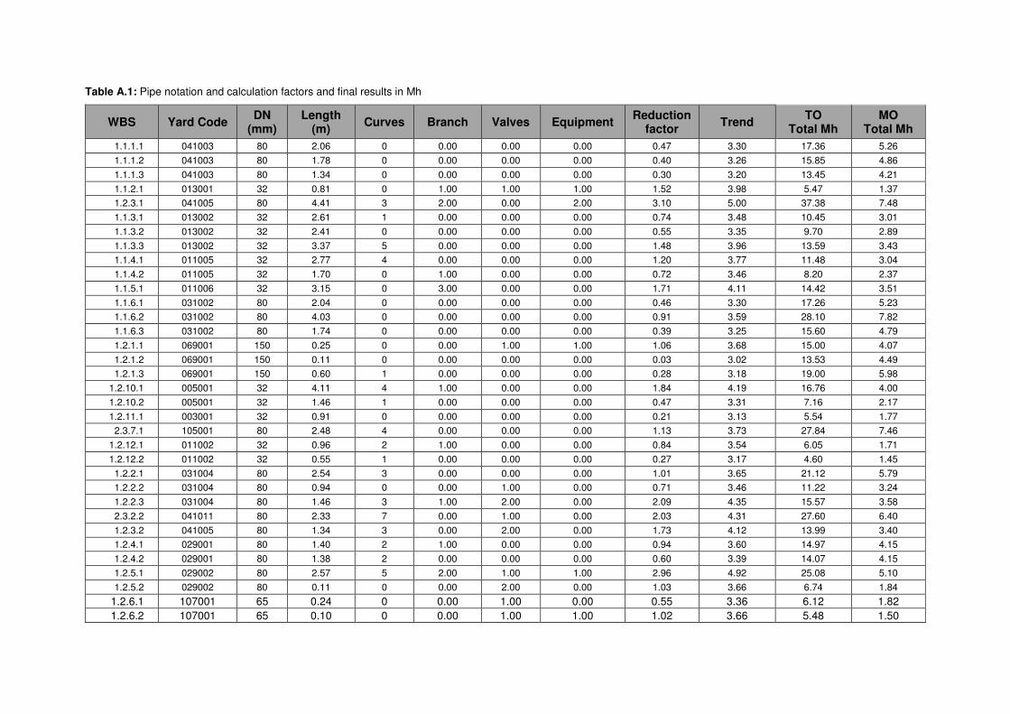
Table A.1: Pipe notation and calculation factors and final results in Mh

WBS Yard Code DN

(mm) Length

(m) Curves Branch Valves Equipment

Reduction factor

Trend TO

Total Mh MO

Total Mh

1.1.1.1 041003 80 2.06 0 0.00 0.00 0.00 0.47 3.30 17.36 5.26

1.1.1.2 041003 80 1.78 0 0.00 0.00 0.00 0.40 3.26 15.85 4.86

1.1.1.3 041003 80 1.34 0 0.00 0.00 0.00 0.30 3.20 13.45 4.21

1.1.2.1 013001 32 0.81 0 1.00 1.00 1.00 1.52 3.98 5.47 1.37

1.2.3.1 041005 80 4.41 3 2.00 0.00 2.00 3.10 5.00 37.38 7.48

1.1.3.1 013002 32 2.61 1 0.00 0.00 0.00 0.74 3.48 10.45 3.01

1.1.3.2 013002 32 2.41 0 0.00 0.00 0.00 0.55 3.35 9.70 2.89

1.1.3.3 013002 32 3.37 5 0.00 0.00 0.00 1.48 3.96 13.59 3.43

1.1.4.1 011005 32 2.77 4 0.00 0.00 0.00 1.20 3.77 11.48 3.04

1.1.4.2 011005 32 1.70 0 1.00 0.00 0.00 0.72 3.46 8.20 2.37

1.1.5.1 011006 32 3.15 0 3.00 0.00 0.00 1.71 4.11 14.42 3.51

1.1.6.1 031002 80 2.04 0 0.00 0.00 0.00 0.46 3.30 17.26 5.23

1.1.6.2 031002 80 4.03 0 0.00 0.00 0.00 0.91 3.59 28.10 7.82

1.1.6.3 031002 80 1.74 0 0.00 0.00 0.00 0.39 3.25 15.60 4.79

1.2.1.1 069001 150 0.25 0 0.00 1.00 1.00 1.06 3.68 15.00 4.07

1.2.1.2 069001 150 0.11 0 0.00 0.00 0.00 0.03 3.02 13.53 4.49

1.2.1.3 069001 150 0.60 1 0.00 0.00 0.00 0.28 3.18 19.00 5.98

1.2.10.1 005001 32 4.11 4 1.00 0.00 0.00 1.84 4.19 16.76 4.00

1.2.10.2 005001 32 1.46 1 0.00 0.00 0.00 0.47 3.31 7.16 2.17

1.2.11.1 003001 32 0.91 0 0.00 0.00 0.00 0.21 3.13 5.54 1.77

2.3.7.1 105001 80 2.48 4 0.00 0.00 0.00 1.13 3.73 27.84 7.46

1.2.12.1 011002 32 0.96 2 1.00 0.00 0.00 0.84 3.54 6.05 1.71

1.2.12.2 011002 32 0.55 1 0.00 0.00 0.00 0.27 3.17 4.60 1.45

1.2.2.1 031004 80 2.54 3 0.00 0.00 0.00 1.01 3.65 21.12 5.79

1.2.2.2 031004 80 0.94 0 0.00 1.00 0.00 0.71 3.46 11.22 3.24

1.2.2.3 031004 80 1.46 3 1.00 2.00 0.00 2.09 4.35 15.57 3.58

2.3.2.2 041011 80 2.33 7 0.00 1.00 0.00 2.03 4.31 27.60 6.40

1.2.3.2 041005 80 1.34 3 0.00 2.00 0.00 1.73 4.12 13.99 3.40

1.2.4.1 029001 80 1.40 2 1.00 0.00 0.00 0.94 3.60 14.97 4.15

1.2.4.2 029001 80 1.38 2 0.00 0.00 0.00 0.60 3.39 14.07 4.15

1.2.5.1 029002 80 2.57 5 2.00 1.00 1.00 2.96 4.92 25.08 5.10

1.2.5.2 029002 80 0.11 0 0.00 2.00 0.00 1.03 3.66 6.74 1.84

1.2.6.1 107001 65 0.24 0 0.00 1.00 0.00 0.55 3.36 6.12 1.82

1.2.6.2 107001 65 0.10 0 0.00 1.00 1.00 1.02 3.66 5.48 1.50

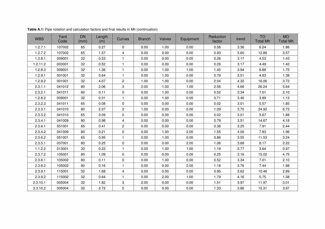
Table A.1: Pipe notation and calculation factors and final results in Mh (continuation)

WBS Yard Code

DN (mm)

Length (m)

Curves Branch Valves Equipment Reduction

factor trend

TO Total Mh

MO Total Mh

1.2.7.1 107002 65 0.27 0 0.00 1.00 0.00 0.56 3.36 6.24 1.86

1.2.7.2 107002 65 1.57 4 0.00 0.00 0.00 0.93 3.60 12.86 3.57

1.2.8.1 009001 32 0.53 1 0.00 0.00 0.00 0.26 3.17 4.53 1.43

1.2.11.2 003001 32 0.52 1 0.00 0.00 0.00 0.26 3.17 4.49 1.42

1.2.8.3 009001 32 1.36 1 0.00 1.00 1.00 1.45 3.94 6.88 1.75

1.2.9.1 001001 32 0.64 1 0.00 1.00 0.00 0.79 3.51 4.83 1.38

1.2.9.2 001001 32 4.07 2 1.00 1.00 0.00 2.04 4.32 16.06 3.72

2.3.1.1 041012 80 2.06 3 2.00 1.00 1.00 2.56 4.66 26.24 5.64

2.3.2.1 041011 80 0.11 0 0.00 1.00 0.00 0.52 3.34 7.01 2.10

1.2.8.2 009001 32 0.31 1 0.00 1.00 0.00 0.71 3.46 3.89 1.13

2.3.2.3 041011 65 0.08 0 0.00 0.00 0.00 0.02 3.01 5.57 1.85

2.3.3.1 041010 80 2.07 2 1.00 0.00 0.00 1.09 3.70 24.92 6.73

2.3.3.2 041010 65 0.09 0 0.00 0.00 0.00 0.02 3.01 5.67 1.88

2.3.4.1 041009 80 0.98 4 0.00 0.00 0.00 0.79 3.51 14.67 4.18

2.3.6.1 051001 65 0.41 2 0.00 0.00 0.00 0.38 3.25 7.91 2.44

2.3.4.2 041009 80 0.21 0 0.00 1.00 2.00 1.55 4.00 7.83 1.96

2.3.6.2 051001 65 0.95 1 0.00 1.00 0.00 0.86 3.55 11.53 3.24

2.3.5.1 037001 80 0.25 0 0.00 0.00 2.00 1.06 3.68 8.17 2.22

1.1.2.2 013001 32 0.22 1 0.00 1.00 1.00 1.19 3.77 3.64 0.97

2.3.7.2 105001 80 1.09 0 0.00 0.00 0.00 0.25 3.16 15.02 4.75

2.3.8.1 105002 80 0.11 0 0.00 1.00 0.00 0.52 3.34 7.01 2.10

2.3.8.2 105002 80 0.16 1 0.00 0.00 2.00 1.18 3.76 7.44 1.98

2.3.9.1 115001 32 1.68 4 0.00 0.00 0.00 0.95 3.62 10.46 2.89

2.3.9.2 115002 32 0.64 1 0.00 2.00 1.00 1.79 4.16 5.75 1.38

2.3.10.1 005004 32 1.82 3 2.00 0.00 0.00 1.51 3.97 11.97 3.01

2.3.10.2 005004 32 2.72 5 0.00 0.00 0.00 1.33 3.86 15.31 3.97

B

8 Annex

Space relationship diagrams

C

9 Annex

Risk analysis and risk responses

Table C.1: Impact factors computed by Guedes Soares and Gomes Lopes method [15]

WBS Identified Risk Objectives Quality Time Cost Impact Factor Quality Delay Costs

1 DESIGN

1.1 Poor identification of equipment and outfitting components forming in modular block x x 0 3 3 6

1.2 Lack of preliminary and further studies in outfitting modular implementation strategy x x 0 2 2 4

1.3 Unexperienced designers on conceptual production manufacturing x x 0 2 1 3

1.4 New procedures and techniques x 0 1 1

1.5 Inadequate working plans, production and detail drawings x x 0 2 3 5

1.6 Inadequate inspection and control methodology x x x 3 1 1 5


2.1 Equipment and raw material delivery out of date x 0 2 0 2

2.2 Piping elements and structural elements, out of forms and dimensions x x 3 2 0 5

2.3 Welding joints faults x x 3 1 0 4

2.4 Equipment delivery without running tests x x 0 2 2 4

3 MODULE ASSEMBLY

3.1 Parts out of dimensions x x x 3 2 1 6

3.2 Parts out of shapes x x x 3 2 1 6

3.3 Components missing x 0 3 0 3

3.4 Components missaligned x x 0 3 0 3


4.1 Module isometric check points out of tolerance in the three-dimensional measurement x 3 0 3

4.2 Hydraulic tests failure due to leakages x x 2 2 0 4


5.1 Overloading for available hoisting equipment x x 0 1 2 3

5.2 Laid-up and laid-down small failures x 0 1 0 1

5.3 Handling operation performed without qualified people x x 3 2 0 5

5.4 Misjudgment of boundary spaces offsets (interferences) x x x 2 1 1 4

5.5 Schedule coordination between Block and Module Block failue x x 0 3 3 6

5.6 Components damages x x 0 2 1 3

6 ON BLOCK ASSEMBLING

6.1 Parts out of dimensions x x x 3 2 1 6

6.2 Parts out of shapes x x x 3 2 1 6

6.3 Components missing x 0 3 0 3

6.4 Block isometric check points for installing block module out of tolerances x x 1 2 0 3

6.5 Block isometric check points for piping connection out of tolerances x x 1 2 0 3

7 FINAL TRIALS FAILURE x x 0 2 2 4

Table C.2: Risk Response Acceptance (A), Mitigation (M), Transfer (T) and Avoidance (I).

CRITICAL SUCCESS FACTORS

1 DESIGN Likelihood Impact Risk Factor Risk Response

F1 1.1 Poor identification of equipment and outfitting components forming in modular block 2 5 10 M

F6 F7 1.2 Lack of preliminary and further studies in outfitting modular implementation strategy 4 4 16 M

F2 1.3 Unexperienced designers on conceptual production manufacturing 2 3 6 M 1.4 New procedures and techniques 2 1 2 A

F2 1.5 Inadequate working plans, production and detail drawings 4 5 20 T

F2 1.6 Inadequate inspection and control methodology 1 5 5 M


F3 F4 2.1 Equipment and raw material delivery out of date 5 2 10 M

F8 F9 2.2 Piping elements and structural elements, out of forms and dimensions 1 5 5 M

F8 F9 2.3 Welding joints faults 2 4 8 M

F8 F9 2.4 Equipment delivery without running tests 1 4 4 M

3 MODULE ASSEMBLY

F8 F9 3.1 Parts out of dimensions 1 5 5 M

F8 F9 3.2 Parts out of shapes 1 5 5 M

F3 F4 3.3 Components missing 3 3 9 M

F8 F9 3.4 Components misaligned 3 3 9 M


F8 F9 4.1 Module isometric check points out of tolerance in the three-dimensional measurement 5 3 15 M

F8 F9 4.2 Hydraulic tests failure due to leakages 4 4 16 M


F8 F9 5.1 Overloading for available hoisting equipment 2 3 6 M

F8 F9 5.2 Laid-up and laid-down small failures 2 1 2 A

F8 F9 5.3 Handling operation performed without qualified people 2 5 10 M

F8 F9 5.4 Misjudgment of boundary spaces offsets (interferences) 4 4 16 M

F8 F9 F3 F4 5.5 Schedule coordination between Block and Module Block failue 5 5 25 I

F8 F9 5.6 Components damages 5 3 15 M

6 ON BLOCK ASSEMBLING 6.1 Parts out of dimensions 4 5 20 T

F8 F9 6.2 Parts out of shapes 4 5 20 T

F8 F9 6.3 Components missing 4 3 12 M

F8 F9 6.4 Block isometric check points for installing block module out of tolerances 4 3 12 M

F8 F9 F8 F9 6.5 Block isometric check points for piping connection out of tolerances 4 3 12 M

F8 F9 7 FINAL TRIALS FAILURE 2 4 8 M

Production methodologies applied to the fluid system ...

Documents

Transcript of Production methodologies applied to the fluid system ...