Production-Inventory Systems with Imperfect Advance Demand

Information and Updating

Saif Benjaafar∗ William L. Cooper∗ Setareh Mardan†

October 25, 2010

Abstract

We consider a supplier with finite production capacity and stochastic production times. Cus-tomers provide advance demand information (ADI) to the supplier by announcing orders aheadof their due dates. However, this information is not perfect, and customers may request an orderbe fulfilled prior to or later than the expected due date. Customers update the status of theirorders, but the time between consecutive updates is random. We formulate the production-control problem as a continuous-time Markov decision process and prove there is an optimalstate-dependent base-stock policy, where the base-stock levels depend upon the numbers oforders at various stages of update. In addition, we derive results on the sensitivity of the state-dependent base-stock levels to the number of orders in each stage of update. In a numericalstudy, we examine the benefit of ADI, and find that it is most valuable to the supplier whenthe time between updates is moderate. We also consider the impact of holding and backordercosts, numbers of updates, and the fraction of customers that provide ADI. In addition, we findthat while ADI is always beneficial to the supplier, this may not be the case for the customerswho provide the ADI.

Keywords: Advance demand information, production-inventory systems, make-to-stock queues,continuous-time Markov decision processes

∗Program in Industrial and Systems Engineering, University of Minnesota, 111 Church Street S.E., Minneapolis,

MN 55455†PROS, 3100 Main Street, Suite #900, Houston, TX 77002

1 Introduction

It is increasingly common for members of the same supply chain to share advance demand infor-

mation (ADI). This practice has been facilitated by information technologies such as the Internet,

electronic data interchange (EDI), and radio frequency identification (RFID). It has also been sup-

ported by initiatives such as the inter-industry consortium on Collaborative Planning, Forecasting

and Replenishment (CPFR), which provides a framework for participating companies to share fu-

ture demand projections and coordinate ordering decisions. Large manufacturers, such as Toyota

and Boeing, are tightly integrated with their first tier suppliers with whom they share produc-

tion status, inventory usage, and even future design plans. Large retailers, such as Wal-Mart and

Best Buy, have invested in sophisticated information collecting and processing infrastructure that

enables them to share real-time inventory usage and point-of-sale (POS) data with thousands of

their suppliers. Several manufacturers that sell directly to the consumer, such as Dell, and online

retailers, such as Amazon, encourage their customers to place their orders early by offering dis-

counts to those that accept later delivery dates. In some industries, suppliers allow their long-term

customers to place soft orders far ahead of due dates, which may then later be firmed up, modified,

or canceled.

Although ADI can take on different forms and may be enabled by a variety of technologies, it

typically reduces to customers providing advance notice to their suppliers about the timing and

size of future orders. This information can be perfect (exact information about future orders) or

imperfect (estimates of timing or quantity of future orders). The information can also be explicit,

with customers directly stating their intent about future orders, or implicit, with customers allowing

suppliers to observe their internal operations and to determine estimates of future orders (the

systems we consider in this paper are in part motivated by settings with such implicit information;

we provide examples and further discussion later in this section). It is generally believed that

ADI, even if imperfect, can improve supply chain performance. In particular, with information

about future demand, a supplier may be able to reduce the need for inventory or excess capacity.

Customers may also benefit through improved service quality or lower costs.

However, the availability of ADI raises questions. How should a supplier use ADI to make

decisions? How valuable is ADI to suppliers and customers and how is this value affected by

operating characteristics of the supplier and the quality of information provided by customers?

How significant are benefits from receiving information further in advance or increasing the portion

of customers that provide ADI? Is ADI equally beneficial to all parties in the supply chain and

could it be harmful, particularly to the customer who provides it?

1

We address these and other related questions for a supplier that produces a single product.

Customers furnish the supplier with ADI by announcing orders ahead of their due dates. However,

this information is not perfect, and orders may become due prior to or later than the announced

expected due date or they can be canceled altogether. Hence, the demand leadtime (the time be-

tween when an order is announced and when it is requested or canceled) is random. Customers

provide status updates as their orders progress towards becoming due, but the time between con-

secutive updates is also random and independent of updates for other orders. In this paper, we are

primarily motivated by settings where customers implicitly provide ADI to the supplier by allowing

the supplier to observe their internal operations (e.g., order fulfillment, manufacturing, inventory

usage), thereby enabling the supplier to estimate when customers will eventually place orders. We

refer to such internal operations as the demand leadtime system.

For most of the paper, we assume that the actual due dates of different orders are independent

of each other and orders that are announced later can become due before (or after) those that are

announced earlier. Updates are also independent and do not follow a first-announced, first-updated

rule. We refer to this as a system with independent due dates (IDD). In Section 5, we show how our

treatment can be extended to systems where announced orders are updated and the orders become

due in the sequence in which they are announced. We refer to this as a system with sequential due

dates (SDD).

The following examples illustrate the types of settings we model in this paper. Consider a sup-

plier that provides a component to a manufacturer, such as Boeing, of a large and complex product

(e.g., an aircraft). The manufacturer informs the supplier each time it initiates the production of a

new product and each time it completes a stage of the production process. The component provided

by the supplier is not immediately needed and is required only at a later stage of the production

process. The manufacturer does not accept early deliveries, but wishes to receive the component as

soon as it is needed in a just-in-time fashion. The supplier uses the information about the progres-

sion of the product through the manufacturer’s production process to estimate when it will need

to make a delivery to the manufacturer. To make such estimates, the supplier uses its knowledge

of the manufacturer’s operations and available data from past interactions. However, the estimates

are imperfect and the manufacturer (due to inherent variability) may complete a production stage

sooner or later than expected. The manufacturer may initiate, in response to its own demand,

the production of multiple products simultaneously (e.g., an aircraft manufacturer may assemble

multiple airplanes in parallel). The evolution of these products through the production process

is largely independent, so that a product that enters a particular stage of production later than

2

another product may complete it sooner.

This type of ADI may also arise in settings other than manufacturing. For example, van

Donselaar et al. (2001) present a case study of how builders provide material suppliers with ADI

about the start and progress of construction projects. The suppliers use the information to estimate

when a builder will need materials. This estimation is not perfect because progress on a construction

project can be variable and because design specifications may change over the course of a project,

sometimes leading the builders ultimately not to place orders.

In this paper, we provide a general framework for modeling systems with this type of ADI.

The framework is broad enough to model a wide range of demand leadtime systems with various

assumptions regrading due date updating. The demand leadtime system can be viewed in general

as a queueing system composed of parallel servers, with service times consisting of multiple stages

of random duration and the completion of a stage of corresponding to an update. Arrivals to the

demand leadtime system correspond to orders being announced; similar to service times, interarrival

times are random and may have multiple stages, with the completion of a stage indicating an update.

Departures from the demand leadtime system correspond to orders becoming due.

In the systems we study, the supplier has finite capacity, producing items one at a time with

stochastic production times. Hence, the supplier itself can be viewed as a single server queue, with

arrivals corresponding to orders becoming due (i.e., an arrival to the supplier is a departure from

the demand leadtime system). The supplier has the ability to produce items ahead of their due

dates in a make-to-stock fashion. However, items in inventory incur a holding cost. When an order

becomes due and it cannot be immediately satisfied from inventory, it is backordered but it incurs

a backorder cost. The supplier’s objective is to find a production control policy to minimize the

expected total discounted cost or the expected average cost per unit time.

We formulate the problem as a continuous-time Markov decision process (MDP). We show that

there is an optimal production policy that is a state-dependent base-stock policy, wherein the supplier

produces if and only if the net inventory is below a base-stock level, which depends only upon the

numbers of orders in various stages of update. We also derive results on the sensitivity of the state-

dependent base-stock levels to the numbers of orders in each stage of update. For SDD systems,

we obtain similar results. In our analysis, we develop a method for proving structural properties of

optimal policies of continuous-time Markov decision processes (CTMDPs) with unbounded jump

rates. The derived structure is useful as it allows one to compute and store an optimal policy

in terms of just the base-stock levels, simplifying the policy’s implementation. The structure of

the optimal policy can also guide construction of simpler heuristics if needed, or in assessing the

3

effectiveness of heuristics that may already be in use.

We also conduct a numerical study to examine the benefits of ADI to both suppliers and

customers by comparing systems with ADI, without ADI, and with partial ADI. The study yields

several managerial insights, a few of which we now summarize. Increasing the average demand

leadtime by increasing the number of updates always reduces the supplier’s cost. However, given

a fixed number of updates, increasing the average time between updates may increase or decrease

cost. ADI is most valuable when the average time between updates is moderate. ADI is less valuable

when the average time between updates is short, because there is little time to react to information.

It is also less valuable when the average time between updates is long, because the earlier notice

comes with an increase in variability of the demand leadtime. This points out that obtaining earlier

notice (on average) of orders is not necessarily desirable, and that when evaluating the benefit of

ADI, it is important to account for the mechanism by which this ADI might be obtained. The

incremental cost reduction from updating is often small compared to that from announcing orders

ahead of their due dates. Typically, much of the benefit of ADI can be realized if customers provide

just initial advance order announcements and few or no updates. Although ADI leads to an overall

reduction in cost, in some cases it may be used by the supplier to reduce inventory at the expense

of more backorders. Therefore, customers that provide ADI may witness a decline in service levels.

However, in exchange for ADI, customers are in position to negotiate an increase in the backorder

penalty they apply to the supplier. Higher backorder penalties can serve as a mechanism for

customers to deter suppliers from reducing service levels, or as a mechanism to share, indirectly,

the cost savings from ADI.

The remainder of the paper is organized as follows. In Section 2, we give a brief literature

review and summarize our contribution. In Section 3, we formulate the problem and describe the

structure of an optimal policy. We also discuss extensions including systems with variable numbers

of updates, order cancelations, multiple customer classes, and lost sales. In Section 4, we present

numerical results. In Section 5, we extend our analysis to systems with sequential updating. In

Section 6, we offer a summary and concluding comments. Proofs are in the Appendix and Online

Supplement.

2 Literature Review and Summary of Contributions

There is a growing literature on inventory systems with ADI. A review of much of this work can

be found in Gallego and Ozer (2002). Models can be broadly classified into two categories based

on whether inventory is reviewed periodically or continuously.

4

For systems with periodic review, ADI is typically modeled as information available about

demand in future periods. Under varying assumptions, Gallego and Ozer (2001), Ozer and Wei

(2004), and Schwarz et al. (1997) have shown the existence of optimal state-dependent base-stock

policies for periodic-review problems with ADI. In these papers, the base-stock levels depend upon

a vector of advance orders for future periods. Ozer (2003) extends the analysis to distribution

systems with multiple retailers, Gallego and Ozer (2003) to serial systems, and Wang and Toktay

(2008) to systems with flexible delivery. Other papers that consider periodic review systems with

ADI include Thonemann (2002), Gavirneni et al. (1999), and DeCroix and Mookerjee (1997).

For continuous-review inventory systems with ADI, Buzacott and Shanthikumar (1994) consider

production-inventory systems with ADI and evaluate policies that use two parameters: a base-stock

level and a release leadtime. Hariharan and Zipkin (1995) introduced the notion of demand leadtime

in a system where orders are announced a fixed amount of time before they are due. For constant

supply leadtimes and Poisson order arrivals, they show that there is an optimal base-stock policy

with a fixed base-stock level. Karaesmen et al. (2002) analyze a discrete-time model with constant

demand leadtimes that is similar to our SDD model with no due-date updating (see Section 5). They

prove the optimality of state-dependent base-stock policies. Gallego and Ozer (2002, Section 2.4)

consider a system similar to a special case of our SDD setting, but with exogenous load-independent

supply leadtimes. Gayon et al. (2009) study a system similar to our IDD scheme but with multiple

demand classes, lost sales, and no due-date updates. Other papers that deal with continuous-review

systems include Liberopoulos et al. (2003) and Karaesmen et al. (2004).

It is possible to view the demand leadtime system in our model as a Markovian demand-

modulating process with transition probabilities between states determined by the dynamics of

order announcements and due dates. Previous literature (see, e.g., Chen and Song 2001) has estab-

lished the optimality of state-dependent base-stock policies for periodic review inventory problems

with Markov-modulated demand and exogenous leadtimes. The results of Chen and Song do not

directly apply to our setting of endogenous leadtimes and continuous review. Nevertheless, it might

be possible to develop an alternate analysis of the systems considered herein using techniques from

the study of inventory models with Markov-demand demand.

Advance demand information can be viewed as a form of forecast updating. Examples of papers

that deal with inventory systems with periodic forecast updates include Graves et al. (1986), Heath

and Jackson (1994), Gullu (1996), Sethi et al. (2001), Zhu and Thonemann (2004), and references

therein. The models we present in this paper can be viewed as dealing with forecast updates.

However, in our case the updates are with respect to the timing of future demand.

5

Finally, there is a literature that deals with how a supplier should quote delivery leadtimes to

its customers; see, for example, Duenyas and Hopp (1995), Hopp and Sturgis (2001), and references

therein. The setting studied in this literature is quite different from ours and typically concerns

make-to-order systems where no finished goods inventory is held in advance of customer orders.

Relative to the above literature, we make the following contributions. Our paper is the first

to consider imperfect ADI with updates for continuous-review production-inventory systems. It

also appears to be the first to directly model stochastic demand leadtimes and distinguish between

systems with independent and sequential due date updates, and to derive the structure of an optimal

policy for each. The paper offers one of the most general models of ADI in the literature (e.g.,

systems with no updates or with a single update can be treated as special cases). The modeling

framework is flexible and can accommodate additional features such as random numbers of updates,

order cancelations, multiple demand classes, and lost sales. Moreover, the numerical study yields

new insights on the benefit of ADI to suppliers, highlighting important effects due to capacity,

demand leadtime, and cost parameters. It also contrasts the impact of (i) increasing the number of

updates, (ii) increasing the fraction of customers who give ADI, and (iii) increasing the length of

individual update stages. The numerical results also shed light on effects of ADI on customers. We

show that customers may see their service quality deteriorate if they provide ADI to their suppliers.

Beyond the context of ADI, our paper also contains an approach for proving structural properties

of optimal policies of CTMDPs with unbounded jump rates. (The IDD model has unbounded jump

rates.) The usual approach for proving structural properties for CTMDPs with bounded jump

rates is to first uniformize (see, e.g., Lippman 1975) the CTMDP to get an equivalent discrete-

time Markov decision process (DTMDP), and then to show that certain properties of functions

are preserved by the DTMDP transition operator. Results then follow using induction and the

convergence of value iteration. With unbounded jump rates, uniformization cannot be applied, and

hence the “usual approach” does not work. Our method for CTMDPs with unbounded jump rates

involves proving the desired structural properties for each of a sequence of problems with bounded

jump rates, and then extending to the problem with unbounded jump rates by passing to a limit

via a suitably chosen subsequence and appealing to results of Guo and Hernandez-Lerma (2003).

Although the method is somewhat intuitive, it involves resolving a number of non-trivial technical

issues, some of which are problem specific. A variant of the approach was used in the paper by

Gayon et al. (2009) cited above. The approach may prove useful in other problems with unbounded

jump rates.

6

3 Problem Formulation and Structure of an Optimal Policy

Consider a supplier of a single product, who can produce at most one unit of the product at a time.

The supplier may hold completed units of the product in inventory. Any such unit of inventory

incurs a holding cost of h per unit time.

We model ADI through the notion of a demand leadtime system. (As mentioned in the in-

troduction, such a system may represent the internal operations of customers; ADI is provided

implicitly by allowing the supplier to view these internal operations.) Orders for the product are

announced before their due dates. Such announcements may be viewed as arrivals to the demand

leadtime system. We assume that the announcements arrive continuously over time according to

a Poisson process with rate λ. The amount of time between when an order is announced and

when it becomes due is random. We refer to this random variable as the demand leadtime. The

demand leadtime of an order is the amount of time it spends in the demand leadtime system. We

assume orders are homogeneous in the sense that demand leadtimes have the same distribution for

all orders, and hence the expected demand leadtime is the same for all orders.

After an order is announced, it progresses through the demand leadtime system before becoming

due. Specifically, it undergoes a series of k − 1 updates (k ≥ 1). For i = 1, . . . , k − 1, the time

between the (i− 1)th and ith update is exponentially distributed with mean ν−1i . (The 0th update

is the order’s initial announcement.) The time between the (k − 1)th update and when the order

becomes due is exponentially distributed with mean ν−1k . Hence, each demand leadtime consists

of k exponentially distributed stages with the expected demand leadtime of each order equal to

ν−11 + · · · + ν−1

k . (The case with k = 1 represents a situation with no updates and exponential

demand leadtimes.) When an order has undergone exactly i − 1 updates we say that it is in stage

i. Viewed in this fashion, the ith update corresponds to an order moving from stage i to stage

(i + 1). When an order undergoes its ith update, the supplier learns that the order’s expected

remaining demand leadtime has decreased from ν−1i + · · · + ν−1

k to ν−1i+1 + · · · + ν−1

k . Equivalently,

we may think of demand leadtime as having a phase-type distribution with k phases in series.

Information is provided each time the demand leadtime completes a phase. In the case where

νi = ν for i = 1, . . . , k, demand leadtimes have an Erlang distribution. Note that the process by

which orders are announced, updated, and become due can be viewed as an M/G/∞ queue.

After an order becomes due (i.e., after it leaves the demand leadtime system), the supplier fills

the order if it has inventory on hand. If the supplier does not have inventory on hand, then the order

is backordered and incurs a backorder cost of b per unit time. Orders do not incur backorder costs

before they are are due; i.e., orders in the demand leadtime system do not incur backorder costs.

7

As mentioned above, the supplier can produce one item at a time. We assume that production

times are exponentially distributed with mean µ−1. Hence, the production process can itself be

viewed as a queue, whose input is provided by the output of the demand leadtime system.

The assumptions of Poisson arrivals of announcements and exponential production and update

times are made in part for mathematical tractability as they allow the problem to be cast as a CT-

MDP. They are also appropriate for approximating systems with high variability. Such Markovian

assumptions are consistent with previous studies of production-inventory systems; see e.g., Buza-

cott and Shanthikumar (1993), Ha (1997), Zipkin (2000), de Vericourt et al. (2002), and others.

Later, we partially relax these assumptions.

In the remainder of this section, we develop the formulation and describe the structure of the

optimal policy. This is done by first analyzing in Section 3.1 a simplified version (with a truncated

state space) of the problem. We then extend the analysis in Section 3.2 to systems without the

truncation and state our main result for this section in Theorem 2.

3.1 Bounded Jump Rates

In this section, we assume that the total number of announced orders (i.e., the number of orders

in the demand leadtime system) at any instant remains bounded by a finite integer m < ∞,

so that∑k

i=1 yi ≤ m, where yi is the number of orders in stage i. Order announcements are

rejected and leave without entering the leadtime demand system (and hence never become due) if∑k

i=1 yi = m. This assumption allows us to formulate the problem as a Markov decision process

with bounded jump rates. From a queueing perspective, the introduction of the finite m means

that we approximate the M/G/∞ queue mentioned above by an M/G/m/m queue (an Erlang loss

system). When m is chosen to be large, very few order announcements are rejected and hence the

arrival rate of due orders to the production facility will be roughly the same as the arrival rate of

order announcements to the demand leadtime system. In fact, the precise arrival rate of due orders

to the production facility will be λ(1 − B(m)) where B(m) is the probability that an M/G/m/m

queue is full. The probability B(m) approaches 0 as m → ∞. The exact value of B(m) is given

by the well-known Erlang loss formula. Using the results of this section as a building block, in

Section 3.2 we extend our results to the case with no bound on the total announced orders.

Let Z and Z+ be respectively the sets of integers and non-negative integers, and let Zk and Z

k+

be their k-dimensional cross products. Let R be the real numbers. Throughout, y = (y1, . . . , yk).

The MDP has state space Sm := Z × Zk+(m), where Z

k+(m) := {y ∈ Z

k+ :

∑ki=1 yi ≤ m}. To

keep notation clean, we will indicate the dependence on m only in notation that is used later for

8

extending to the case without m. It is, however, important to keep in mind that most of the

quantities in this section do depend upon m, even if this is not reflected in the notation.

The state of the system is determined by X(t), which represents the net inventory at time t,

and Y(t) = (Y1(t), . . . , Yk(t)), where Yi(t) is the number of announced orders in stage i at time t.

In each state, two actions are possible: produce or idle (do not produce). The objective is to

find a production policy that minimizes the long-run expected discounted cost. Let the set of such

production policies be denoted by Π. A deterministic stationary policy π := {π(x,y) : (x,y) ∈ Sm}

specifies the action taken at any time as a function only of the state of the system, where π(x,y) = 1

means produce in state (x,y), and π(x,y) = 0 means idle in state (x,y).

We will work with a uniformized version (see, e.g., Lippman, 1975) of the problem in which the

transition rate in each state under any action is Λ := λ+µ+m∑k

i=1 νi so that the transition times

0 = τ0 ≤ τ1 ≤ τ2 ≤ . . . are such that {τn+1 − τn : n ≥ 0} is a sequence of i.i.d. exponential random

variables, each with mean Λ−1. Let {(Xn,Yn) : n ≥ 0} denote the embedded Markov chain of

states; that is, (Xn,Yn) := (X(τn),Y(τn)) is the state immediately after the n-th transition. For

i = 1, . . . , k, let ei be the k−dimensional vector with 1 in position i and zeros elsewhere. Let e0

be the k-dimensional vector of zeros. If action a ∈ {0, 1} is selected in state (x,y), then the next

state of the embedded Markov chain is (x′,y′) with probability

p(x,y),(x′,y′)(a) :=

Λ−1µI{a=1} if (x′,y′) = (x + 1,y)

Λ−1λI{y<m} if (x′,y′) = (x,y + e1)

Λ−1νiyiI{yi≥1} if (x′,y′) = (x,y + ei+1 − ei)

Λ−1νkykI{yk≥1} if (x′,y′) = (x − 1,y − ek)

Λ−1[Λ − µI{a=1} − λI{y<m} −

∑ki=1 νiyiI{yi≥1}

]if (x′,y′) = (x,y)

0 otherwise,

where y :=∑k

i=1 yi and I{·} is the indicator function. The cost rate when the state is (x,y) is

c(x,y) = c(x) := hx+ + bx−, where h > 0 and b > 0 are the per-unit holding and backorder cost

rates, and x+ = max{x, 0} and x− = −min{x, 0}. Here, we again emphasize that backorder costs

are incurred only when an order becomes due and is not immediately satisfied. Jobs inside the

demand leadtime system (which have been announced, but which are not yet due) do not incur

backorder costs.

The value function, which specifies the optimal expected total discounted cost, is given by

v∗m(x,y) := infπ∈Π

Eπ(x,y)

[ ∫ ∞

t=0e−βtc(X(t))dt

]= inf

π∈ΠEπ

(x,y)

[∞∑

n=0

(Λ

γ

)n c(Xn)

γ

], (1)

9

where β > 0 is the discount rate, γ := β + Λ, and Eπ(x,y) denotes expectation with respect to the

probability measure determined by policy π and (X(0),Y(0)) = (x,y).

Let V be the set of real-valued functions on Sm and let v be an arbitrary element of V . Define

Tλ, T ′i , Tµ : V → V as follows

Tλv(x,y) := v(x,y + e1I{y<m})

T ′iv(x,y) := v(x,y + [ei+1 − ei]I{yi≥1}) i = 1, . . . , k − 1 (2)

T ′kv(x,y) := v(x − I{yk≥1},y − ekI{yk≥1}) (3)

Tµv(x,y) := min{v(x,y), v(x + 1,y)}.

Consider also the operator T : V → V defined by

Tv(x,y) := mina∈{0,1}

{c(x)

γ+

Λ

γ

∑

(x′,y′)∈S

p(x,y),(x′,y′)(a)v(x′,y′)

}(4)

= γ−1[c(x) + λTλv(x,y) +

k∑

i=1

νiyiT′iv(x,y) +

k∑

i=1

νi(m − yi)v(x,y) + µTµv(x,y)]. (5)

The function v∗m defined in (1) is the minimum non-negative solution of the optimality equation

v = Tv, (6)

and moreover a stationary policy that specifies for each (x,y) an action that attains the minimum

on the right-hand side of (6) is optimal. See, e.g., Section 11.5 of Puterman (1994).

In the optimality equation (6), operator Tλ corresponds to the arrival of a customer. More

precisely, if v(x,y) represents the “value” of being in state (x,y), then Tλv(x,y) is the value just

after an arrival occurs when the state is (x,y). Similarly, operator T ′i ; i = 1, . . . , k − 1 corresponds

to an update of an order from stage i to stage i + 1 and operator T ′k corresponds to an order

becoming due. Operator Tµ corresponds to the production decision. When v(x + 1,y) < v(x,y),

it is better to produce a unit of inventory than it is to idle. In this case Tµv(x,y) = v(x + 1,y)

represents the value just after the completion of the unit of inventory when the state is (x,y). When

v(x + 1,y) ≥ v(x,y), it is instead better to idle, in which case Tµv(x,y) = v(x,y). The other term

—∑k

i=1 νi(m − yi)v(x,y) — in the optimality equation corresponds to null transitions introduced

through uniformization of the jump rate. To understand the term λ that multiplies Tλv(x,y), note

that in state (x,y), the next event will be an arrival with probability λ/Λ. Similar interpretations

are possible for the other multipliers. The term λ also represents the rate of order announcements.

Likewise, µ is the rate of potential production completions, νiyi is the rate of updates at stage i

10

when yi orders are in stage i, and∑k

i=1 νi(m− yi) is the rate of null transitions when there y jobs

in the demand leadtime system. Hence Λ is the overall rate of (real and null) transitions.

In preparation for Theorem 1, let ∆v(x,y) := v(x + 1,y)− v(x,y) for v ∈ V and let U := {v ∈

V : v satisfies conditions (C1)–(C4)}, where conditions (C1)–(C4) are defined as follows:

(C1) ∆v(x,y) ≤ ∆v(x + 1,y) for all x ∈ Z, y ∈ Zk+(m).

(C2) ∆v(x,y + ej) ≤ ∆v(x + 1,y + el) for all x ∈ Z, y ∈ Zk+(m − 1), j = 0, . . . , k − 1, and

l = j + 1, . . . , k.

(C3) ∆v(x,y + ej+1) ≤ ∆v(x,y + ej) for all x ∈ Z, y ∈ Zk+(m − 1), and j = 0, . . . , k − 1.

(C4) ∆v(x,y) ≤ 0 for all x ∈ Z with x < 0, y ∈ Zk+(m).

As we can see from Proposition 1 below, the value function satisfies these conditions. The fact that

the value function satisfies these conditions implies certain structural properties for the optimal

policy. In particular, Condition (C1) is a convexity property that can be used to show the existence

of a state-dependent base-stock optimal policy. Conditions (C2) and (C3) can be used to show that

the announcement of a new order or the update of an existing order will cause the base-stock level

either to increase by one or to remain unchanged. Condition (C4) can be used to show that it is

optimal to produce whenever there are backorders.

Proposition 1 The value function is an element of U ; that is, v∗m ∈ U .

The proof of Proposition 1 is in Section S-1 of the Online Supplement. We are now ready for

the main result of the section. Theorem 1 describes the structure of an optimal policy; a proof is

in the appendix.

Theorem 1 The stationary state-dependent base-stock policy π∗ = {π∗(x,y)} given by

π∗(x,y) :=

0 if x ≥ sy

1 if x < sy

(7)

where sy := min{x : v∗m(x + 1,y) − v∗m(x,y) ≥ 0} is optimal. In addition, (a) the base-stock levels

satisfy sy+el∈ {sy+ej

, sy+ej+1} for j = 0, . . . , k−1; l = j +1, . . . , k and (b) π∗(x,y) = 1 if x < 0.

Theorem 1 states that for each vector y of announced orders there exists a threshold sy such that

it is optimal to produce if net inventory is less than sy, and it is optimal to idle if net inventory is

at least sy. We refer to the parameters {sy} as the y-dependent base-stock levels. Part (a) with

11

l = j + 1 indicates that the y-dependent base-stock level increases by at most one if an order is

updated or if a new order is announced. It also follows from part (a) that sy is increasing in each

component of y; i.e., sy ≤ sy+iejfor i ∈ Z+ and j = 1, . . . , k. Part (b) states that it is optimal to

produce if there are any backorders. These results are consistent with those obtained by Ozer and

Wei (2004), who show a similar structure to the optimal policy in periodic-review systems where

ADI consists of confirmed demand for future periods (e.g., see Theorem 2 in Ozer and Wei 2004).

Figure 1 illustrates the structure described in Theorem 1 for two examples, each with k = 2

stages. In part (a) of the figure, the mean time 1/νi spent in each of the stages is relatively long,

and hence the production policy is much less sensitive to orders in stage 1 than it is to orders in

stage 2. In part (b) the mean time 1/νi is shorter, and hence the production policy treats orders

in stage 1 almost the same as orders in stage 2.

020

4060

80

0

20

40

60

800

20

40

60

80

100

120

140

Announced orders in stage 2, y 2

Announced orders in stage 1, y1

Net

inve

ntor

y x

(a) ν1 = ν2 = 0.01 (b) ν1 = ν2 = 0.10

Figure 1: Optimal policies for two different systems with IDD and k = 2: The surfaces

depict the state-dependent base-stock levels. For a given y = (y1, y2), if the net inventory

on hand x is below the surface, it is optimal to produce; if the net inventory on hand x is

on or above the surface, it is optimal to idle. (m = 200, µ = 1, λ = 0.6, h = 10, b = 100)

Above, we focused on the discounted-cost optimality criteria. A treatment of average cost can

be found in Section S-2 of the Online Supplement, where Theorem S-1 shows that a direct analog

of Theorem 1 holds for the average-cost optimality criteria under the additional assumption that

λ < µ (which ensures that production can keep up with demand and prevent backorders from

growing “infinitely large”). In the discounted-cost case, we do not need this assumption.

We close this section by illustrating the flexibility of our modeling framework in accommodating

additional features. In particular, we consider four extensions to our basic model: (1) systems with

12

random numbers of updates, (2) systems with order cancelations, (3) systems with two demand

classes, one providing ADI and the other one not, and (4) systems with lost sales.

Systems with Random Numbers of Updates. Suppose that customers update their orders

a random number of times. In particular, suppose that given an announced order is at stage i, it

will, independent of everything else, become due after the end of stage i with probability qi and

progress to next stage with probability 1 − qi, for i = 1, . . . , k − 1. To extend the model to a such

setting with a random number of updates, we need to replace T ′i in (5) by T ′

i defined by

T ′iv(x,y) := (1 − qi)T

′iv(x,y) + qiv(x − I{yi≥1},y − eiI{yi≥1}) i = 1, . . . , k . (8)

In this case, there is again an optimal state-dependent base stock policy and it is optimal

to produce whenever backorders are present. However, to prove properties (a) and (b) of the

base-stock levels in Theorem 1 we impose the condition that ν1q1 ≤ ν2q2 ≤ · · · ≤ νkqk; that is,

νiqi is non-decreasing in i. A proof is in Section S-3 of the Online Supplement. To understand

the importance of this condition, suppose temporarily that the condition does not hold. More

specifically, suppose, e.g., that ν1q1 is much larger than ν2q2. Then an order in stage 1 is, in a

sense, “closer” to becoming due than is an order in stage 2. To see this, observe that an order in

stage 1 tends to quickly become due after just one stage of update whereas, in the event that the

order progresses to stage 2, it tends to remain there a (relatively) long time. Hence, there may

be (x,y) such that it is best to produce when in state (x,y + e1), but best to idle when in state

(x,y + e2).

Systems with Order Cancelations. In some settings, customers may cancel their orders after

they have been announced. For example, consider a situation where, with each update, an order is

either canceled or its due date is updated. In this case, ADI is imperfect with regard to both timing

and realization of future orders. For example, in the context of a building construction project,

changes to building specifications at some stage of the project may lead the builder to cancel orders

for certain material. To incorporate this into the model, let pi now denote the probability that an

order is canceled at the end of its ith stage. The case where pi = 0 corresponds to a system with

no cancelations. The state space, action space, and cost rates are as in a system without order

cancelations. To handle cancelations, we need only replace T ′i in (5) by

T ′iv(x,y) := (1 − pi)T

′iv(x,y) + piv(x,y − eiI{yi≥1}) i = 1, . . . , k .

See Section S-4 of the Online Supplement for a proof that Theorem 1 holds for systems with order

cancelations under the additional assumption that νipi is non-increasing in i.

13

Systems with two Customer Classes. In some situations, it may be the case that not all

customers provide ADI. In other words, there may be a fraction of customers that does not announce

orders ahead of demand. This is plausible in settings where the supplier has a mix of long-term and

short-term (or non-recurring) customers. Long-term customers are more likely to share information

and to invest in the necessary infrastructure. Suppose that a fraction η of orders provides ADI,

and that a fraction 1 − η does not. Equivalently, we may view customers as belonging to two

separate classes. Class 1, with arrival rate λ1 = ηλ, provides ADI, and Class 2, with arrival rate

λ2 = (1 − η)λ, does not. To incorporate this into the model, we replace the operator Tλ by

Tλv(x,y) := ηTλv(x,y) + (1 − η)v(x − 1,y) .

The operator Tλ preserves conditions (C1)–(C4) because Tλ does; see the proof of Proposition 1.

Hence, Theorem 1 holds in this setting.

Systems with Lost Sales. So far we have assumed that when orders become due and there is

no on-hand inventory, orders can wait. In many applications, orders cannot wait and instead are

lost if they become due and cannot be filled immediately. With each lost order, a lost sales cost

is incurred. This cost may be a negotiated penalty with the customer or may reflect the cost of

expediting the order or fulfilling it from an outside supplier (it may also reflect the loss of good

will). To incorporate lost sales, we need only take the state space to be Z+ × Zk+(m), re-define the

cost function to be c(x) = hx, and replace the operator T ′k by T ′

k defined as follows:

T ′kv(x,y) := v([x − I{yk≥1}]

+,y − ekI{yk≥1}) + cLSI{yk≥1 and x=0}, (9)

where cLS corresponds to the lost sale cost per unit. Section S-5 of the Online Supplement contains

a proof that Theorem 1 [except property (b), which pertains to backorders] holds in this setting.

3.2 Unbounded Jump Rates

In this section we again consider the basic IDD system under the discounted-cost criterion. The

model is identical to that considered in the previous section, except that here we do not place the

bound m on the number of announced orders in the system. There are no rejected orders, and all

arrivals enter the demand leadtime system. The state space is now S := Z × Zk+. Without the

bound m, we have a continuous-time Markov decision process with unbounded transition rates.

In particular, the conditional rate of transitions out of state (x,y) ∈ S under action a ∈ {0, 1} is

λ +∑k

i=1 νiyi + µI{a=1}. With no bound m on∑k

i=1 yi, this conditional rate is not bounded.

Theorem 2 below shows that the results in Theorem 1 also hold in the setting with unbounded

jump rates (and discounted costs). We conjecture that similar results for unbounded jump rates

14

hold under the average-cost criterion, but we do not have a proof at this time. Although this

may not be surprising because Theorem 1 holds for any finite m, it is important to highlight

that the presence of unbounded transition rates poses a technical challenge. In particular, it is

not possible to apply uniformization to a problem with unbounded jump rates, and hence the

problem cannot be transformed into an “equivalent” discrete-time problem as in Section 3.1. Such

a transformation is typically a crucial step for proving structural properties of optimal policies

using inductive approaches (as in the proof of Proposition 1). An additional difficulty is that only

recently has there developed a theory for problems with both unbounded jump rates and unbounded

cost rates that characterizes the value function as a particular solution of the optimality equation,

and ensures the existence of stationary optimal policies. See Guo and Hernandez-Lerma (2003) —

hereafter called GH — for results and references.

Our proof of Theorem 2 establishes the structure of an optimal policy and of the value function

for the problem with unbounded jump rates by letting m grow to infinity through a particular

sequence of problems such as those considered in Section 3.1. In doing so, there are a number

of technical points, such as the existence of various limits, that must be treated with care. The

approach may provide a template that could be used for analyzing other CTMDPs with unbounded

jump rates and cost rates.

Let v∗ denote the value function of the problem with unbounded jump rates. The optimality

equation for the problem with unbounded jump rates is v = Lv, where L is given by

Lv(x,y) :=1

Q(y)

[c(x) + λv(x,y + e1) +

k∑

i=2

νi−1yi−1v(x,y + ei − ei−1)

+ νkykv(x − 1,y − ek) + µ min{v(x,y), v(x + 1,y)}]

and Q(y) := β + λ +∑k

i=1 νiyi + µ.

In preparation for the main theorem of the section, define function R(·) by

R(x,y) := |x| +

k∑

i=1

yi (10)

and consider the set of functions BR(S) := {v : there exist constants c1, c2 ≥ 0 so that |v(x,y)| ≤

c1 + c2R(x,y) for all (x,y) ∈ S} where R(x,y) is given in (10). To employ the theory of GH, we

must identify a non-negative function R suitable for defining BR(S). GH do not specify an R for

the use of their theory. “Suitable” means that R must satisfy some conditions that relate to the

cost and transition rates of the CTMDP. In Lemma S-2 in Section S-6 of the Online Supplement we

verify that our choice of R in (10) is indeed suitable. For convenience, Section S-6 also summarizes

results we use from GH.

15

The following is the main result of the section. A proof is in the appendix.

Theorem 2 For the system with IDD and unbounded jump rates, the value function v∗ is the unique

function in BR(S) that solves the optimality equation v = Lv. Moreover, v∗ satisfies conditions

(C1)–(C4), and there exists a stationary state-dependent base-stock policy that is optimal. The

base-stock levels satisfy the conditions in (a) and (b) in Theorem 1.

4 Numerical Results

In this section, we present results from a numerical study. The goal is to examine the benefits from

using ADI, to assess the value of updating, and to compare the impact of having full versus partial

ADI. The insights we obtain for production-inventory systems with continuous review complement

results in the literature for systems with periodic review and deterministic leadtimes.

We use average cost instead of discounted cost, because average cost is independent of the initial

state and the discount factor. In all cases we set ρ = λ/µ < 1, so that Theorem S-1 applies (see

Section S-2 of the Online Supplement). The holding-cost rate is h = 10 and the production rate

is µ = 1, unless stated otherwise. In the numerical study, we used values of m large enough that

further increases in m would not alter the average costs at the level of accuracy shown in our tables.

For each problem instance, we obtained the long-run average cost by solving the MDP using value

iteration.

4.1 Benefits of ADI

To assess the benefit of ADI, we compare the optimal average cost, JA, for a system with ADI to

the optimal average cost, JN , for a system with no ADI and obtain the percentage cost reduction

PCR := 100 × (JN − JA)/JN . The two systems are identical in all respects, except that in the

system with no ADI, orders are not announced ahead of their due dates; rather, information about

when orders enter the demand leadtime system and when they move from one stage to the next

is withheld. Only departures from the last stage of the demand leadtime system are observed. In

general, the distribution of the departure process from the demand leadtime system is different

from the distribution of its arrival process. However, the arrival and departure processes in steady

state have identical (Poisson with rate λ) distributions for systems with no bound m. This follows

from the fact that the departure process from an M/G/∞ queue in steady state is a homogeneous

Poisson process with the same rate as the exogenous input Poisson process. For systems with finite

m, the departure process in steady state is closely approximated by a Poisson process when m is

16

large.

Long-run average cost is unaffected by the transient behavior of the demand leadtime system. As

the demand leadtime system approaches steady state, its departure process converges in distribution

to a Poisson process with rate λ. Hence, we may, for the purpose of computing long-run average

cost for a system without ADI, assume arrivals to the system without ADI form a Poisson process.

Finally, we note that a (state-independent) base-stock policy is optimal for a system with no ADI

with Poisson arrivals and exponential production times; see, e.g., Veatch and Wein (1996).

Representative numerical results comparing systems with and without ADI can be found in

Table 1, where PCR is shown for varying values of parameters ν, λ, and b. The results are shown for

a system with a single stage (k = 1). The effect of multiple update stages is discussed in Section 4.2.

ν

λ 0.01 0.02 0.05 0.1 0.2 0.5 1 2 5 10

0.1 0.00 0.00 0.00 0.02 0.37 3.94 8.07 17.84 12.60 7.53

0.2 0.00 0.00 0.06 0.64 2.36 8.39 14.11 18.41 11.74 6.84

0.4 0.51 1.66 4.84 8.52 12.73 16.21 20.97 17.74 9.60 5.35

b = 10 0.6 0.84 2.45 6.13 9.46 12.03 12.82 9.81 1.38 1.08 0.81

0.8 6.04 8.47 10.54 10.61 9.06 5.87 3.26 2.02 0.54 0.04

0.9 9.02 9.25 7.58 5.37 3.03 1.21 1.17 1.03 0.99 0.92

0.1 0.36 1.96 8.01 16.33 25.47 44.92 40.43 28.71 14.76 8.12

0.2 3.06 6.18 12.88 20.44 28.61 38.63 28.61 13.15 0.38 0.29

0.4 5.15 7.57 12.41 17.58 22.52 17.64 15.29 10.67 5.17 2.74

b = 50 0.6 4.24 7.58 12.88 15.46 14.77 7.77 4.75 1.51 0.86 0.47

0.8 11.19 13.77 13.29 9.87 5.95 2.59 1.31 0.89 0.38 0.16

0.9 11.73 12.78 5.30 2.74 1.14 0.44 0.23 0.20 0.13 0.02

0.1 8.93 14.28 23.84 32.73 49.49 51.82 39.08 23.15 6.63 0.05

0.2 0.13 1.08 6.14 13.96 25.43 18.72 6.63 5.90 3.11 1.55

0.4 2.08 4.78 10.96 16.58 19.37 15.63 5.06 4.07 2.06 1.04

b = 100 0.6 5.85 9.72 15.17 16.82 13.96 6.95 3.14 1.89 0.86 0.52

0.8 12.93 14.98 12.63 8.04 4.42 1.64 0.83 0.46 0.24 0.13

0.9 9.85 10.09 6.98 4.01 2.03 0.41 0.23 0.20 0.12 0.03

Table 1: The percentage cost reduction (PCR) for a system with k = 1.

The effect of ν on PCR, when all other parameter values are fixed, is not monotonic, with

PCR initially increasing in the mean demand leadtime 1/ν and then decreasing. ADI offers the

greatest benefit in terms of PCR when the size of 1/ν is moderate. The percentage cost reduction

is relatively small when either 1/ν is very large or very small. This can be explained as follows.

17

When 1/ν is small, the mean time between when an order is announced and when it becomes due

is small. Hence, the information is of little use. When 1/ν is large, the mean of the time between

an order’s announcement and due date is large, but so is the variance. This makes the information

about future demand relatively less useful. The meanings of “large,” “small,” and “moderate” 1/ν

depend upon the value of λ. Although the joint effect of λ, µ, and ν on PCR is complicated, it

appears that the value of 1/ν that maximizes PCR for a given λ is increasing in λ. The largest

value of 1/ν shown in Table 1 is 1/ν = 100; however, computations for larger values support the

claim that the relative benefit of ADI is small for large 1/ν. For instance, with b = 100, λ = 0.8,

and 1/ν = 500, we find that PCR is 3.22. These results highlight an important insight: having

earlier notice of future orders may not always be desirable since the quality of this information tends

also to deteriorate (i.e., the variance in the demand leadtime increases when the average demand

leadtime increases). In our model, this is due to the fact that demand leadtime is assumed to have

the exponential distribution. However, this also captures the fact that in practice the earlier an

order is announced, the less reliable will be the estimate of its due date (see Section 4.2 for further

results and discussion for systems with multiple stages of updating).

For each fixed ν, the effect of λ on PCR is also not monotonic. For fixed ν, the relative benefit

of ADI is small when λ is large (close to µ = 1). When λ is large, the optimal policy with or

without ADI is for the production facility to produce most of the time. Hence, the availability of

ADI makes little difference for the decisions taken. When λ is small, the absolute cost reduction

from ADI is small, because costs in the systems with and without ADI both approach zero as λ ↓ 0,

but the value of PCR depends on the value of ν; see Section S-7 of the Online Supplement for

further discussion on this.

The effect of the ratio b/h is also not monotonic, with the value of PCR relatively small when

b/h is either small or large. When b/h is small, ignoring ADI and producing to order (i.e., holding

little or no inventory in anticipation of future demand) carries a relatively small penalty. When b/h

is large, the base-stock levels are high for systems both with and without ADI, and the probability

of backorders is relatively small in both systems. Hence, ADI becomes relatively less useful.

We conclude this section by comparing the preceding observations with those obtained by

Gavirneni et al. (1999), who also evaluated the benefit of ADI with respect to similar parameters,

but in a different context. They study a periodic review system with zero leadtimes and limited

replenishment capacity per period, where ADI is obtained by having the supplier observe the

demand of a retailer that uses an (s, S) ordering policy. Some of their qualitative insights (for

example, regarding the effect of the ratio b/h) are similar to those above. However, there are

18

some notable differences. For example, they found that the percentage cost reduction due to ADI

is increasing in capacity. Interestingly, Ozer and Wei (2004), who consider a different model of

capacitated periodic-review inventory systems with ADI, concluded the opposite. That is, in their

modeling framework, they found ADI to be most beneficial when capacity is tight. Both of these

findings can be contrasted to the effect of varying λ (which varies production system loading) that

we describe above.

Some effects observed in both Gavirneni et al. (1999) and in our study appear to have different

causes in the different settings. For instance, they find that long demand leadtimes (measured in

their case by the difference S − s) diminish the value of ADI, and they attribute this to the fact

that long leadtimes result in large orders from the retailer, forcing the supplier to build inventory

over time because of capacity limits. In our case, long demand leadtimes also diminish the value of

ADI, but for a different reason: the information regarding due dates becomes less reliable because

both the mean and the variance of demand leadtime increase simultaneously.

4.2 Benefits of Updating

In settings where the demand leadtime system consists of multiple stages, the supplier and customer

may have a choice of how much information is shared. For example, should the customer inform

the supplier as soon as an order enters the first stage or wait until an order has progressed further

before forwarding the information to the supplier? Similarly, should the customer update the

supplier each time an order enters a new stage or should it wait until the order has passed a

specified number of stages? These questions are relevant when there is a cost associated with

collecting the information, transmitting it from one party to another, and then making decisions

based on it. To explore the benefit of full versus partial information sharing, we consider a system

where the demand leadtime has two stages (k = 2) and compare the performance of this system

when there is full ADI (information is shared as soon as orders enter the first stage and as they

leave one stage and enter the next) to its performance when there is no ADI and when there is

only partial ADI (information is shared only when orders enter the second stage). The systems

can be viewed as identical in all respects except for the number of update stages, with full ADI

corresponding to k = 2, partial ADI to k = 1, and no ADI to k = 0. In the system with full

ADI, the order is announced and then progresses through two stages of update, each exponentially

distributed with mean 1/ν, before becoming due. In the system with partial ADI, the order is

announced and then progresses through a single stage of update, exponentially distributed with

mean 1/ν, before becoming due. In the system with no ADI, the order is announced and becomes

19

due immediately.

Representative numerical results are displayed in Table 2, which not surprisingly shows that full

ADI is superior. (A proof of this observation follows by noting that any policy for the system with

partial ADI can be reproduced for the system with full ADI by basing decisions in the latter only

on the net inventory and the number of orders in the second stage.) Additional numerical results

for b = 10 and b = 50 can be found in Section S-9 of the Online Supplement. The value of full ADI

is most significant when both ν and λ are in the mid-range, and least significant when both ν and

λ are either very small or very large, as in the upper left and lower right corners of Table 2. This

is consistent with results from Section 4.1. In most of the examples considered, the incremental

benefit from full ADI (k = 2) over partial ADI (k = 1) is small. This suggests that partial ADI

may be sufficient if updating is expensive to implement.

We close this section by noting a subtle difference between the effect of increasing ADI by

increasing the number of stages observable to the supplier and increasing ADI by increasing the

length of a particular stage. Compare a system with k stages in which each stage has mean 1/ν to

a system with a single stage with mean k/ν. Both systems have the same overall mean, k/ν, but

the variance of the system with k stages is k/ν2 while the one for the system with a single stage is

k2/ν2 (i.e., k times larger). This helps explain why observing more stages of the demand process

is always beneficial, but increasing the average length of a particular stage may not be.

4.3 Benefits of Full versus Partial ADI

As discussed at the end of Section 3.1, there are settings where ADI is not available from all

customers. An important question that arises in these settings is how beneficial is it to increase the

fraction of customers that provide ADI. In particular, is there a diminishing value to increasing this

fraction or is the marginal benefit from ADI insensitive to how many customers already provide

ADI? To address this question, we consider the version of our problem where there are two customer

classes described at the end of Section 3.1. Class 1, with demand rate λ1 = ηλ, provides ADI and

class 2, with demand rate λ2 = (1− η)λ, does not. We examine the effect of increasing the fraction

of customers with ADI by varying the fraction η while maintaining λ = λ1 + λ2 constant, so that

higher values of η correspond to more customers providing of ADI.

Representative results from numerical experiments are shown in Figure 2 (with k = 1, λ = 0.8,

and b = 100). As we can see in this example, the relative benefit of ADI does not exhibit diminishing

returns with increases in the fraction η of customers with ADI. (The “nearly linear” pattern in the

figure is present for other parameter settings as well. In some cases it is less pronounced.) This

20

λ = 0.4 λ = 0.6 λ = 0.8

ν1 = ν2 k=0 k=1 k=2 k=0 k=1 k=2 k=0 k=1 k=2

0.01 25.07 24.55 24.53 46.38 43.67 43.65 107.24 93.38 92.10

2.08% 2.14% 5.85% 5.90% 12.93% 14.12%

0.02 25.07 23.87 23.85 46.38 41.87 41.74 107.24 91.18 87.81

4.78% 4.86% 9.72% 10.00% 14.98% 18.12%

0.05 25.07 22.32 22.26 46.38 39.35 38.47 107.24 93.70 86.93

10.96% 11.21% 15.17% 17.06% 12.63% 18.94%

0.10 25.07 20.91 20.40 46.38 38.58 36.60 107.24 98.62 91.50

16.58% 18.62% 16.82% 21.10% 8.04% 14.69%

0.20 25.07 20.21 19.00 46.38 39.91 36.33 107.24 102.51 98.04

19.37% 24.20% 13.96% 21.68% 4.42% 8.58%

0.50 25.07 21.15 18.60 46.38 43.16 39.82 107.24 105.49 103.47

15.63% 25.80% 6.95% 14.14% 1.64% 3.52%

1.00 25.07 23.80 20.62 46.38 44.93 43.05 107.24 106.35 105.48

5.06% 17.75% 3.14% 7.18% 0.83% 1.65%

1.50 25.07 23.90 22.65 46.38 45.38 43.93 107.24 106.68 105.90

4.66% 9.64% 2.16% 5.30% 0.53% 1.26%

2.00 25.07 24.05 23.63 46.38 45.51 44.89 107.24 106.75 106.33

4.07% 5.74% 1.89% 3.22% 0.46% 0.85%

Table 2: Average cost and percentage cost reduction (PCR) for systems with b = 100. The

columns labeled “k = 0” show the average cost for systems without ADI.

is in contrast to the typical effect of updating. These differences might, in part, be due to the

fact that with additional updating we provide more information for the same customers while

with expanding ADI to additional customers we provide new information for different customers.

This is significant since we assume that customers announce orders independently of each other,

so having information on some customers does not provide information on when other customers

might announce their own orders. A managerial implication from these observations is that, all else

being equal, and given our independence assumptions, a supplier may be better off expanding ADI

(with limited or no updating) to more of its customers than obtaining more updates from those

customers that already provide ADI.

These results appear to be different from those reported in the literature for systems with

periodic review. For example, Ozer and Wei (2004) carried out a set of experiments where they

varied the number of periods ahead of due dates that demand is announced (they refer to this as

the information horizon), as well as the effective fraction of customers that announce their demand

21

0 0.1 0.2 0.3 0.4 0.5 0.6 0.7 0.8 0.9 10

2

4

6

8

10

12

14

η

Perc

enta

ge C

ost R

educ

tion

(PC

R)

ν = 0.05ν = 0.1ν = 0.2ν = 0.5ν = 1

Figure 2: PCR versus fraction of customers

that provide ADI.

1005020105210.50.20.128

30

32

34

36

38

40

42

44

46

48

1/ ν

Ave

rage

cos

t

Holding cost (no ADI)Holding cost (with ADI)Backorder cost (with ADI)Backorder cost (no ADI)

Figure 3: Average holding and backorder

costs, with and without ADI.

ahead of due dates. Their results show a diminishing marginal cost reduction from increasing the

fraction of customers whose demand is announced ahead of its due date. These differences might be

due to the fact that for a continuous review system, production decisions are made for one unit at a

time. Consequently, the system manager is able to use information about the anticipated due date

of each order to make a decision about whether or not to initiate the production of a replenishment

unit.

4.4 Benefits of ADI to the Customer

In evaluating the benefit of ADI, we have so far taken the perspective of the supplier who manages

the production process. In this section, we consider the impact of ADI on the customer who provides

it. In particular, we address the question of whether or not both supplier and customer benefit

from sharing demand information. It is often argued that ADI can reduce costs of the supplier

(which we observed to be true) and improve the quality of service received by the customer. In our

setting, the latter assertion would mean that customers experience fewer backorders and shorter

fulfillment delays. In Figure 3, we show the breakdown of supplier cost in terms of inventory

holding and backorder cost for examples with b = 50. (By Little’s Law, the average waiting time of

customers is proportional to the average backorder cost, so average waiting times can be deduced

from Figure 3. We emphasize that “waiting time” here refers to the span of time between when an

order becomes due and when the order is satisfied. With ADI, an order becomes due when it exits

the demand leadtime system.) As we can see, ADI does not always reduce the backorder costs. In

some cases, the supplier uses ADI to reduce inventory holding cost at the expense of backorder cost.

Generally, whether backorder cost, holding cost, or both decrease (both cannot increase) depends

22

upon problem parameters. Hence, there is no guarantee that sharing ADI will lead to improved

service levels to the customers.

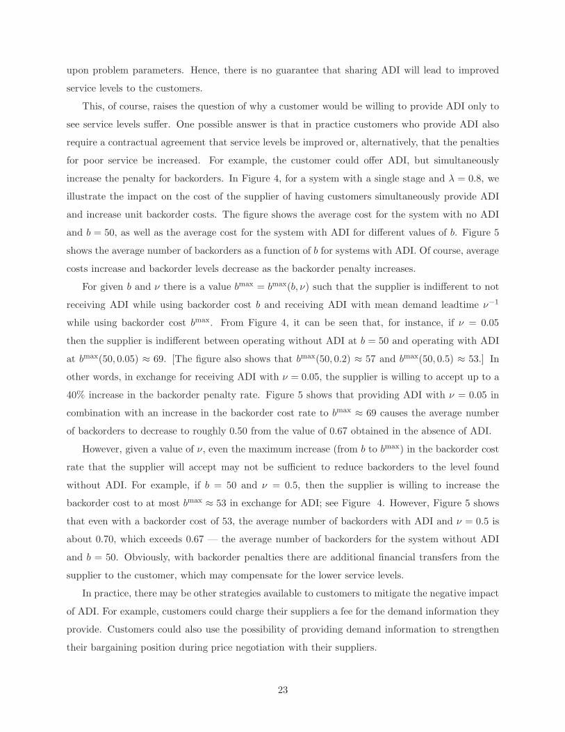
This, of course, raises the question of why a customer would be willing to provide ADI only to

see service levels suffer. One possible answer is that in practice customers who provide ADI also

require a contractual agreement that service levels be improved or, alternatively, that the penalties

for poor service be increased. For example, the customer could offer ADI, but simultaneously

increase the penalty for backorders. In Figure 4, for a system with a single stage and λ = 0.8, we

illustrate the impact on the cost of the supplier of having customers simultaneously provide ADI

and increase unit backorder costs. The figure shows the average cost for the system with no ADI

and b = 50, as well as the average cost for the system with ADI for different values of b. Figure 5

shows the average number of backorders as a function of b for systems with ADI. Of course, average

costs increase and backorder levels decrease as the backorder penalty increases.

For given b and ν there is a value bmax = bmax(b, ν) such that the supplier is indifferent to not

receiving ADI while using backorder cost b and receiving ADI with mean demand leadtime ν−1

while using backorder cost bmax. From Figure 4, it can be seen that, for instance, if ν = 0.05

then the supplier is indifferent between operating without ADI at b = 50 and operating with ADI

at bmax(50, 0.05) ≈ 69. [The figure also shows that bmax(50, 0.2) ≈ 57 and bmax(50, 0.5) ≈ 53.] In

other words, in exchange for receiving ADI with ν = 0.05, the supplier is willing to accept up to a

40% increase in the backorder penalty rate. Figure 5 shows that providing ADI with ν = 0.05 in

combination with an increase in the backorder cost rate to bmax ≈ 69 causes the average number

of backorders to decrease to roughly 0.50 from the value of 0.67 obtained in the absence of ADI.

However, given a value of ν, even the maximum increase (from b to bmax) in the backorder cost

rate that the supplier will accept may not be sufficient to reduce backorders to the level found

without ADI. For example, if b = 50 and ν = 0.5, then the supplier is willing to increase the

backorder cost to at most bmax ≈ 53 in exchange for ADI; see Figure 4. However, Figure 5 shows

that even with a backorder cost of 53, the average number of backorders with ADI and ν = 0.5 is

about 0.70, which exceeds 0.67 — the average number of backorders for the system without ADI

and b = 50. Obviously, with backorder penalties there are additional financial transfers from the

supplier to the customer, which may compensate for the lower service levels.

In practice, there may be other strategies available to customers to mitigate the negative impact

of ADI. For example, customers could charge their suppliers a fee for the demand information they

provide. Customers could also use the possibility of providing demand information to strengthen

their bargaining position during price negotiation with their suppliers.

23

30 40 50 60 70 80 90 100 11050

60

70

80.26

90

100

110

b

Ave

rage

Cos

t

ν = 0.05ν = 0.2ν = 0.5

Average cost for a system without ADI and b=50

Figure 4: Average cost with ADI versus unit

backorder cost rate.

30 40 50 60 70 80 90 100 1100.3

0.4

0.5

0.6

0.670.7

0.8

0.9

1

1.1

1.2

1.3

b

Ave

rage

Num

ber

of B

acko

rder

s

ν = 0.05ν = 0.2ν = 0.5

Average number of backorders without ADI and b=50

Figure 5: Average number of backorders ver-

sus unit backorder cost rate.

5 Extension to Systems with Sequential Due Dates

In this paper, we have focused on a particular form of ADI updating, in which orders that have

been announced are updated independently of each other. In this section we briefly discuss how

our analysis can be extended to systems where the independent updating assumption does not

hold. In particular, we consider a system in which ADI is revealed through a process where

orders are updated and become due in the same order they are announced. We call this a system

with sequential due dates (SDD). Systems with SDD are similar in all aspects to systems we

have considered so far, except for how orders progress through the leadtime system. For example

consider a supplier who produces a component for a manufacturer. The manufacturer’s production

process is a serial production line comprised of a series of workstations that process jobs on a

first-come, first-served (FCFS) basis. If a workstation is busy, incoming jobs wait in its queue. The

manufacturer informs the supplier each time it releases a job to the line (this may correspond to

the manufacturer receiving an order from its own customers) and updates the supplier each time a

job completes processing at one of the workstations. The supplier uses this information to estimate

when it will receive a delivery request from the manufacturer. Such a request coincides with a job

arriving at the workstation where the component provided by the supplier is needed.

SDD may arise in settings other than manufacturing. Consider, for example, a supplier that

produces a product sold through a single retailer, which continuously reviews its inventory and

follows a (Q, r) ordering policy. This means that the retailer places an order for Q units each time

its inventory position drops to r. The supplier has real-time access to retailer’s point-of-sale data

and is aware of the retailer’s ordering policy. Each order placed with the retailer can be used by

the supplier to update its estimate of the time until the next replenishment order. This updating

24

process progresses through Q stages, culminating in the placement of an order for a single batch of

Q units. From the perspective of the supplier, there is always exactly one announced order, whose

due date is updated each time the retailer’s inventory position changes. Once an order becomes

due, another order is simultaneously announced and starts the same process.

In a system with SDD, the leadtime system can be viewed as a serial queueing system consisting

of n servers (we refer to these as nodes). As we shall illustrate with several examples shortly, the

demand leadtime system could describe the internal processes of the customers that are observable

to the supplier. External arrivals to the demand leadtime system occur at node 1 and progress

sequentially through nodes 1, . . . , n. Completion of service at the n-th node corresponds to an

order becoming due. Service time at node i consists of ki stages, with the duration of each stage

being exponentially distributed with mean 1/νij for the j-th stage at node i. That is, service times

at node i have a phase-type distribution with ki phases in series. Special cases include the Erlang

distribution where all the phases have the same mean and the exponential distribution where the

number of phases is equal to one. Orders at each server are processed one at a time on a FCFS

basis.

Inter-arrival times to the demand leadtime system have a phase type distribution, with one or

more phases in series. To describe this arrival process, we introduce an additional node (node 0)

and let k0 denote the number of phases (or stages) associated with this node. The j-th stage in

node 0 has the exponential distribution with mean 1/ν0j for j = 1, ..., k0. Special cases are a Poisson

arrival process or an arrival process with Erlang inter-arrival times.

The state of the system is described by the pair (x,y) where the scalar x represents the net

inventory level and y = (yij : i = 0, . . . , n, j = 1, . . . , ki) represents the state of the demand

leadtime system. For i 6= 0, yij represents the number of orders in node i that are in stage j. For

stage 1, the state variable yi1 indicates the number of orders that are either waiting for service

at node i or have initiated the first stage of service at node i. Therefore, yi1 is a non-negative

integer that can be arbitrarily large. For j 6= 1, yij indicates whether or not there is an order

that has initiated the j-th stage of service. Since servers process units one at a time, there can

be at most one order at a time in stage j 6= 1. Hence, yij is either 0 or 1 for j = 2, . . . , ki and∑ki

j=2 yij ∈ {0, 1}. For node i = 0, y0j is either 0 or 1 and∑k0

j=1 y0j = 1, since there is exactly

one order at node 0 at all times. In summary, the state space is S := Z × Y, where Y := Y0 ∩ Y1,

Y0 := {y : y0j ∈ {0, 1} for j = 1, . . . , k0 and∑k0

j=1 y0j = 1}, and Y1 := {y : yij ∈ Z+ for j =

1, . . . , ki, i = 1, . . . , n and∑ki

j=2 yij ∈ {0, 1} for i = 1, . . . , n}.

It is possible to model a wide variety of settings through different combinations of the parameters

25

ki and n. We describe three examples below.

Example 1. Consider the example described earlier where a supplier provides a component to a

manufacture whose production system consists of a series of workstations. Let production times at

the supplier be exponentially distributed. Let also the manufacturer produce on a make-to-order

basis while facing a Poisson external demand process. The component provided by the supplier

is used in the (n + 1)th workstation and is expected to be delivered by the supplier as soon as

an order goes through the first n workstations. The manufacturer shares information about when

orders are released into the production system and when they complete an operation at any of the

workstations. In our general framework, this system corresponds to ki = 1 for i = 0, . . . , n.

Example 2. Consider a system similar to the one described in example 1, except that items at

the manufacturer are now processed one unit at time with all the operations carried out on a single

workstation (instead of a series of workstations). At any given time, there may be multiple orders

waiting to be processed in the queue of the workstation, but at most one order undergoing pro-

cessing. Each time the workstation completes an operation, the manufacturer informs the supplier.

The manufacturer also informs the supplier each time a new order arrives to the workstation. This

system corresponds to k0 = 1 and n = 1.

Example 3. Consider the example mentioned earlier of a supplier who has a single customer in the

form of a retailer. Let the retailer face a Poisson demand process with rate ν. The retailer uses a

(Q, r) ordering policy so that it places an order of size Q whenever its own inventory position (sum

of inventory on order and inventory on hand less backorders) reaches r. The retailer’s inventory

position takes on values Q+ r,Q+ r−1, . . . , r +1 with transition times between consecutive values

being exponentially distributed with rate ν. If the supplier has access to the retailer’s inventory

position, then the supplier can use the information to update the expected time at which the retailer

will place an order. From the perspective of the supplier there is exactly one announced order at

a time and the time between updates (there is a total of Q updates) is exponentially distributed

with rate ν. In this setting, one “unit” for the supplier is an order of size Q from the retailer and

the production time for this unit is exponential with rate µ. This case corresponds to k0 = Q and

n = 0 with ν0j = ν for j = 1, . . . , k0.

Define eij to be the vector with 1 in the (i, j)-position and zeros elsewhere, and let e00 be the

vector of zeros. Let V be the set of real-valued functions on S. We denote by v∗ ∈ V the value

function of the MDP. That is, v∗(x,y) is the minimum expected total discounted cost, given the

26

system starts in state (x,y). Let γ := µ+∑n

i=0

∑ki

j=1 νij . The optimality equation is v = T v where

T : V → V is defined by

T v(x,y) := γ−1

[c(x) +

n∑

i=0

ki∑

j=1

νijTijv(x,y) + µTµv(x,y)

]. (11)

The operator Tµ corresponds to the production decision and is defined in Section 3.1. The operators

{Tij} in (11) are defined in (12)–(17) below. The operators {T0j : j < k0} correspond to transitions

in the phase of the external arrival process, T0k0corresponds to an external arrival to the demand

leadtime system or to an order coming due in case n = 0, {Tij : i > 0, j < ki} correspond to a

transition in the phase of a service time, and {Tiki: i > 0} correspond to a transition of an order

between nodes (for i < n) and to an order coming due (for i = n). We have

T0jv(x,y) := v(x,y + [e0,j+1 − e0j ]I{y0j=1}) j = 1, . . . , k0 − 1 (12)

T0k0v(x,y) :=

v(x,y + [e01 − e0k0+ e11]I{y0k0

=1}) when n > 0

v(x − I{y0k0=1},y + [e01 − e0k0

]I{y0k0=1}) when n = 0.

(13)

Ti1v(x,y) := v(x,y + [ei2 − ei1]I{yi1≥1 and yiℓ=0 for ℓ=2,...,ki}) i = 1, . . . , n when ki ≥ 2 (14)

Tijv(x,y) := v(x,y + [ei,j+1 − eij]I{yij≥1}) i = 1, . . . , n; j = 2, . . . , ki − 1 (15)

Tikiv(x,y) := v(x,y + [ei+1,1 − eiki

]I{yiki≥1}) i = 1, . . . , n − 1 (16)

Tnknv(x,y) := v(x − I{ynkn≥1},y − enkn

I{ynkn≥1}) . (17)

Note that Ti1 for i = 1, . . . , n is defined by (16)–(17) when ki = 1.

In preparation for our main result of this section, we introduce an ordering on the space of

(node, phase)-indices. For (p, q), (r, w) ∈ {(i, j) : i = 0, . . . , n; j = 1, . . . , ki} ∪ {(0, 0)}, we define

(p, q) ≺ (r, w) to mean that one of the following two conditions holds: (i) p < r, or (ii) p = r and

q < w. Intuitively, (p, q) ≺ (r, w) means that an order at stage w of node r is closer to being due

than an order at stage q of node p. We will use the following analogs of Conditions (C1)–(C4).

(C1) ∆v(x,y) ≤ ∆v(x + 1,y) for all (x,y) ∈ S.

(C2) ∆v(x,y+epq) ≤ ∆v(x+1,y+erw) for all (x,y) and (p, q) ≺ (r, w) such that y+epq, y + erw ∈ Y.

(C3) ∆v(x,y+erw) ≤ ∆v(x,y+epq) for all (x,y) and (p, q) ≺ (r, w) such that y+epq,y+erw ∈ Y.

(C4) ∆v(x,y) ≤ 0 for all (x,y) ∈ S with x < 0.

When n ≥ 1 and k0 ≥ 2 we also use Condition (C5) below, which is related to the “arrival”

node, 0. Condition (C5) is needed to ensure that Condition (C3) is preserved by T ; see the proof

of Proposition S-1 in the Online Supplement. If n = 0 or k0 = 1, then Condition (C5) is vacuous.

27

(C5) ∆v(x,y+e01+e11) ≤ ∆v(x,y+e0q) for all (x,y) and q ≥ 2 such that y+e0q,y+e01+e11 ∈ Y.

The next theorem, which describes the structure of optimal policies for SDD systems, is the

main result of this section. We give a proof in Section S-8 of the Online Supplement. The argument

parallels the proof of Theorem 1 that is detailed in Section 3.1 of the text and in Section S-1 of the

Online Supplement. Specifically, we show that T preserves Conditions (C1)–(C5), which allows us

to conclude that v∗ satisfies Conditions (C1)–(C5), from which the theorem then follows.

Theorem 3 The state-dependent base-stock policy π∗ = {π∗(x,y)} given by

π∗(x,y) :=

0 if x ≥ sy

1 if x < sy

(18)

where sy := min{x : v∗(x + 1,y) − v∗(x,y) ≥ 0} is optimal. In addition, (a) the base-stock levels

satisfy sy+erw ∈ {sy+epq , sy+epq + 1} for (p, q) ≺ (r, w) such that y + epq,y + erw ∈ Y; and (b)

π∗(x,y) = 1 if x < 0.

As we did for systems with independent updating, it is possible to evaluate the benefit of ADI

with SDD features. Table S-3 in the Online Supplement contains numerical results for systems

with SDD, and shows the effects of parameters ν, k, and ρ.

6 Concluding Comments

In this paper, we considered production-inventory systems where the production facility has access

to ADI in the form of advance order announcements and subsequent updates. The ADI is not

perfect because orders may become due before or after announced expected due dates, the time

between updates is random, and announced orders may be canceled. In addition, only a fraction of

the customers may provide ADI. We considered two schemes through which demand information is

revealed, one in which due dates are independent and the other in which they are sequential. For

each scheme, we formulated the production control problem as a continuous-time Markov decision

process and showed that there is an optimal state-dependent base-stock policy, with base-stock

levels that are non-decreasing in the number of announced orders at each stage of update. We also

showed that the base-stock level increases by at most one unit with a unit increase in the number

of orders at any stage.

In numerical experiments, we observed that the cost reduction to the supplier from the intro-

duction of ADI is sensitive to the number of update stages and the length of each stage. Although

28

adding more update stages is always beneficial, increasing the average length of stages may increase

or decrease cost, with ADI being most valuable when the average stage length is moderate. We

also observed that in many cases, much of the benefit of updating can be achieved with one update.

Although ADI is always beneficial to the supplier, we observed that this may not be the case for the

customers who provide the ADI. In some cases, the supplier uses ADI to reduce inventory at the

expense of higher backorders. We showed that a possible remedy is for the customers to negotiate

higher backorder penalties in exchange for ADI.

There are several avenues for future research. It would be of interest to consider systems

where order sizes are variable and where the actual size of an order is not known exactly until the

order becomes due. This would generalize the model with cancelations by assigning a probability

distribution to orders that allows sizes other than zero or one. It would also be of interest to

consider multiple customer classes with differing backorder costs. Although the problem would be

made difficult by the need for a higher-dimensional state space, we expect there would again be an

optimal state-dependent base-stock policy, where the state would include backorder levels of orders

from each customer class. In addition to production, the policy would specify whether an order

that becomes due should be satisfied from available inventory, if there is any, or backordered. This

decision would of course depend on the backorder cost associated with the order’s class.

Appendix

Proof of Theorem 1. Any stationary policy that uses for each (x,y) ∈ Sm an action that attains

the minimum in Tv∗m(x,y) is optimal. Hence, the policy that prescribes action a = 1 in states

S1m := {(x,y) ∈ Sm : v∗m(x + 1,y) < v∗m(x,y)} and action a = 0 in states S0

m := {(x,y) ∈ Sm :

v∗m(x + 1,y) ≥ v∗m(x,y)} is optimal. By Proposition 1, v∗m satisfies Condition (C1), so π∗ defined

in (7) satisfies π∗(x,y) = 1 for (x,y) ∈ S1m and π∗(x,y) = 0 for (x,y) ∈ S0

m. Hence π∗ is optimal.

To prove (a), note that by Proposition 1, the value function v∗m satisfies conditions (C2) and

(C3). Applying condition (C3) l−j times and using the definition of sy+el, we have ∆v∗m(sy+el

,y+

ej) ≥ ∆v∗m(sy+el,y + el) ≥ 0, which implies sy+el

≥ sy+ej. Also, by condition (C2) and the

definition of sy+ej, we have ∆v∗m(sy+ej

+ 1,y + el) ≥ ∆v∗m(sy+ej,y + ej) ≥ 0, which implies

sy+ej+ 1 ≥ sy+el

. Therefore, sy+ej≤ sy+el

≤ sy+ej+ 1 and hence sy+el

is equal to either sy+ej

or sy+ej+ 1. Finally, part (b) is a consequence of the fact that v∗m satisfies condition (C4).

An alternative proof of the optimality of a state-dependent base-stock policy and for part (a) can

be obtained by casting the problem in terms of service rate control and using results on monotone

optimal policies for continuous-time MDPs in Veatch and Wein (1992).

29

Proof of Theorem 2. The first statement follows from Theorem 3.2 of GH. Lemma S-2 in the

Online Supplement shows that the conditions needed to apply their theorem hold for our problem.

For each m, extend the domain of v∗m from Sm to S by defining v∗m(x,y) := 0 for (x,y) ∈ S\Sm.

To prove the remaining statements, we begin by showing that there exists a pointwise convergent

subsequence of {v∗m}. Lemma 1 below implies for each (x,y) ∈ S that {v∗m(x,y)} is a bounded

sequence of real numbers (note that the bound does not depend upon m). Hence, for each (x,y),

the sequence {v∗m(x,y)} has a convergent subsequence in R.

Let {z1, z2, z3, . . . } be an enumeration of the countable space S [each zi is some element (x,y)

of S]. We now proceed with a diagonalization argument to construct the pointwise convergent

subsequence of {v∗m}. Let {m1,j : j = 1, 2, . . .} be such that limj→∞ v∗m1,j(z1) exists. Next, let

{m2,j : j = 1, 2, . . .} be a subsequence of {m1,j : j = 2, 3, . . .} such that limj→∞ v∗m2,j(z2) exists.

Note also that limj→∞ v∗m2,j(z1) exists, because {m2,j : j = 1, 2, . . .} ⊆ {m1,j : j = 2, 3, . . .}.

Continuing in this fashion, we proceed sequentially to extract subsequences of subsequences so

that for each n we have {mn,j : j = 1, 2, . . .} ⊆ {mn−1,j : j = n, n + 1, . . .} and limj→∞ v∗mn,j(zi)

exists for i = 1, . . . , n. Let mj := mj,j. It can now be seen that limj→∞ v∗mjexists pointwise.

(Alternatively, we may appeal to Tychonoff’s Theorem to reach this conclusion; see, e.g., Bremaud

1999.) Let v∗∗ denote the limit; that is, v∗∗ : S → R is defined to be the function for which

limj→∞ v∗mj(x,y) = v∗∗(x,y) for all (x,y) ∈ S.

Next, we show that the limit v∗∗ is in fact the value function v∗ for the problem with unbounded

jump rates. To do so, it will be helpful to re-write the optimality equation (6) from Section 3.1 as

v = Lmv where operator Lm is given by

Lmv(x,y) :=1

Qm(y)

[c(x) + λI{y<m}v(x,y + e1) +

k∑

i=2

νi−1yi−1v(x,y + ei − ei−1)

+ νkykv(x − 1,y − ek) + µ min{v(x,y), v(x + 1,y)}]

and Qm(y) := β + λI{y<m} +∑k

i=1 νiyi + µ. By rearranging terms, it can be checked that the

equation v = Lmv is equivalent to (6). Keep in mind that T in (6) depends upon m.

For any function v on S and any (x,y) ∈ S, observe that Lmv(x,y) = Lv(x,y) if m > y.

Hence, for any (x,y) ∈ S it follows that

v∗∗(x,y) = limj→∞

v∗mj(x,y) = lim

j→∞Lmj

v∗mj(x,y) = lim

j→∞Lv∗mj

(x,y). (19)

For any function v on S and any (x,y) ∈ S we next re-express Lv(x,y). To this end, for given

30

(x,y) consider the continuous function L(x,y) : Rk+3 → R defined by

L(x,y)(ϕ1, . . . , ϕk+3) :=1

Q(y)

[c(x) + λϕ1 +

k+1∑

i=2

νi−1yi−1ϕi + µ min{ϕk+2, ϕk+3}

].

It can now be seen that

Lv(x,y) = L(x,y)

(v(x,y + e1), v(x,y + e2 − e1), . . . , v(x,y + ek − ek−1),

v(x − 1,y − ek), v(x,y), v(x + 1,y))

.

For any sequence of functions {uj} with uj → u pointwise, we have

limj→∞

Luj(x,y) = limj→∞

L(x,y)

(uj(x,y + e1), uj(x,y + e2 − e1), . . . , uj(x,y + ek − ek−1),

uj(x − 1,y − ek), uj(x,y), uj(x + 1,y))

= L(x,y)

(u(x,y + e1), u(x,y + e2 − e1), . . . , u(x,y + ek − ek−1), (20)

u(x − 1,y − ek), u(x,y), u(x + 1,y))

= Lu(x,y) .

Note that in (20), we may pass the limit inside L(x,y) because L(x,y) is continuous. Applying the

preceding observation with {uj} = {v∗mj} and u = v∗∗ and using (19), it follows that v∗∗(x,y) =

Lv∗∗(x,y). Now, because (x,y) was arbitrary, we see that v∗∗ = Lv∗∗. That is, v∗∗ solves the

optimality equation for the problem with unbounded jump rates. Moreover, it can be seen from

Lemma 1 that v∗∗ is in BR(S) with c1 = β−2(h + b)(λ + µ) and c2 = β−1(h + b). Therefore, it

follows from the first part of the theorem that v∗∗ = v∗; that is, v∗∗ is the value function for the

problem with unbounded jump rates. It can now readily be verified that v∗ = limj→∞ v∗mjsatisfies

conditions (C1) through (C4) with Zk+(m − 1) and Z

k+(m) replaced by Z

k+.

Theorem 3.3 of GH implies that the stationary policy that produces in states S1 := {(x,y) ∈

S : v∗(x + 1,y) < v∗(x,y)} and that idles in states S0 := {(x,y) ∈ S : v∗(x + 1,y) ≥ v∗(x,y)}

is optimal for the problem with unbounded jump rates. By an argument identical to the proof of

Theorem 1, such a policy is a state-dependent base-stock policy that satisfies (a) and (b).

Lemma 1 0 ≤ v∗m(x,y) ≤ β−1(h + b)R(x,y) + β−2(h + b)(λ + µ) < ∞, where v∗m is the value

function for the problem with bounded jump rates in Section 3.1 and the function R is defined

in (10).

Proof. Fix m < ∞ and (x,y) ∈ Sm. To bound v∗m(x,y) from above, it suffices to obtain an upper

bound on the expected discounted cost of using the policy π+ that “always produces” [π+(x′,y′) = 1

31

for all (x′,y′) ∈ Sm]. To this end, we begin by developing an explicit construction of a version of

the continuous-time Markov chain (CTMC) induced by π+. Suppose that {Ai : i = 1, 2, . . . } is an

i.i.d. sequence of uniform [0, 1] random variables and that {Ei : i = 1, 2, . . . } is an i.i.d. sequence of

exponential random variables each with mean Λ−1, independent of {Ai : i = 1, 2, . . . }. Let E0 := 0,

En :=∑n

j=1 Ej for n = 1, 2, . . . , and N(t) := max{n ≥ 0 : En ≤ t}.

Recall the notation y′ =∑k

i=1 y′i. Consider the function f : Sm × [0, 1] → Sm given by

f((x′,y′), a) :=

(x′ + 1,y′) if a ∈[0, µ/Λ

]

(x′,y′ + e1I{y′<m}) if a ∈(µ/Λ, (λ + µ)/Λ

]

(x′,y′ + ei+1 − ei) if a ∈((λ + µ +

∑i−1j=1 νjy

′j)/Λ, (λ + µ +

∑ij=1 νjy

′j)/Λ

]

for i = 1, . . . , k − 1

(x′ − 1,y′ − ek) if a ∈((λ + µ +

∑k−1j=1 νjy

′j)/Λ, (λ + µ +

∑kj=1 νjy

′j)/Λ

]

(x′,y′) otherwise.

For the fixed value (x,y) ∈ Sm, define

(X0,Y0) := (x,y) (21)

(Xn,Yn) := f((Xn−1,Yn−1), An) n = 1, 2, . . .

and (X(t),Y(t)) := (XN(t),YN(t)). Note that {(X(t),Y(t)) : t ≥ 0} has the distribution of the

CTMC induced by π+, as desired.

For n = 1, 2, . . . define

Rn :=∣∣∣{j ∈ {1, . . . , n} : (Xj ,Yj) = (Xj−1 + 1,Yj−1)

}∣∣∣

Un :=∣∣∣{j ∈ {1, . . . , n} : (Xj ,Yj) = (Xj−1,Yj−1 + e1)

}∣∣∣

Dn :=∣∣∣{j ∈ {1, . . . , n} : (Xj ,Yj) = (Xj−1 − 1,Yj−1 − ek)

}∣∣∣

where here | · | is set cardinality. When k = 1, it is possible to visualize Rn, Un, and Dn by graphing

the transitions of {(X(t),Y(t))} on a two-dimensional grid. Then, Rn is how many of the first n

transitions are “to the right”, Un is how many of the first n transitions are “up”, and Dn is how

many of the first n transitions are “diagonal”. From the above definitions, note that

Xn = X0 + Rn − Dn and Yn = Y0 + Un − Dn . (22)

(Again, Yn =∑k

i=1 Yn,i.) For n = 1, 2, . . . also define

Un :=∣∣∣{j ∈ {1, . . . , n} : Aj ∈

(µ/Λ, (λ + µ)/Λ

]}∣∣∣ .

32

By construction, we have

Un ≤ Un and Dn ≤ Y0 + Un . (23)

Next we construct another process that is coupled with {(X(t),Y(t))}. Consider the function

g : Z+ × [0, 1] → Z+ given by

g(z, a) :=

z + 1 if a ∈[0, (λ + µ)/Λ

]

z otherwise.

Define

Z0 := |x| + y

Zn := g(Zn−1, An) n = 1, 2, . . . ,

where (x,y) is as in (21) and Z(t) := ZN(t). Observe that

Zn = Z0 + Rn + Un = |x| + y + Rn + Un . (24)

Combining (21)–(24), we get

|Xn| = |X0 + Rn − Dn| ≤ |X0| + Rn + Dn

≤ |X0| + Rn + Y0 + Un

≤ |X0| + Rn + Y0 + Un

= |x| + Rn + y + Un

= Zn.

Hence, |X(t)| ≤ Z(t). Next, define c†(x) := (h + b)x. Note that c(x) ≤ c†(|x|) and that c†(·) is

increasing on Z+. Therefore,

Eπ+

(x,y)

∫ ∞

t=0e−βtc(X(t))dt = E

∫ ∞

t=0e−βtc(X(t))dt ≤ E

∫ ∞

t=0e−βtc†(|X(t)|)dt ≤ E

∫ ∞

t=0e−βtc†(Z(t))dt,

where E is expectation on the probability space upon which {Ai} and {Ei} are defined and where

the initial state is (x,y). Hence, E∫ ∞t=0 e−βtc†(Z(t))dt is an upper bound on v∗m(x,y).

Regardless of m, the process {Z(t)} has the following “dynamics”: Z(0) = |x| + y and Z(·)

remains in state (say) z ∈ Z+ an exponential amount of time with mean 1/(λ + µ) before moving

to state z + 1 ∈ Z+. The latter fact can be verified by conditioning on the geometric number of

transitions made from z back to z by the embedded process {Zn}. Direct calculations using value

33

iteration [to compute the expected discounted cost accrued by {Z(t)} through the time of its (say)

j-th jump to the right] and induction show that

E

∫ ∞

t=0e−βtc†(Z(t))dt =

(h + b)(|x| + y)

λ + µ + β

∑

i≥0

(λ + µ

λ + µ + β

)i

+h + b

λ + µ + β

∑

i≥1

i

(λ + µ

λ + µ + β

)i

=(h + b)(|x| + y)

β+

(h + b)(λ + µ)

β2< ∞ ,

regardless of m. This completes the proof.

References

Bremaud, P., 1999. Markov Chains: Gibbs Fields, Monte Carlo Simulation, and Queues. Springer-

Verlag, New York.

Buzacott, J. A., Shanthikumar, J. G., 1993. Stochastic Models of Manufacturing Systems. Prentice-

Hall, Upper Saddle River, NJ.

Buzacott, J. A., Shanthikumar, J. G., 1994. Safety stock versus safety time in MRP controlled

production systems. Management Science 40, 1678–1689.

Chen, F., Song, J.-S., 2001. Optimal policies for multiechelon inventory problems with Markov-

modulated demand. Operations Research 49, 226–234.

de Vericourt, F., Karaesmen, F., Dallery, Y., 2002. Optimal stock allocation for a capacitated

supply system. Management Science 48, 1486–1501.

DeCroix, G. A., Mookerjee, V. S., 1997. Purchasing demand information in a stochastic-demand

inventory system. European Journal of Operational Research 102, 36–57.

Duenyas, I., Hopp, W. J., 1995. Quoting customer lead times. Management Science 41, 43–57.

Gallego, G., Ozer, O., 2001. Integrating replenishment decisions with advance order information.

Management Science 47, 1344–1360.

Gallego, G., Ozer, O., 2002. Optimal use of demand information in supply chain management. In:

Song, J., Yao, D. (Eds.), Supply Chain Structures: Coordination, Information and Optimization.

Kluwer Academic Publishers, pp. 119–160.

Gallego, G., Ozer, O., 2003. Optimal replenishment policies for multi-echelon inventory problems

under advance order information. Manufacturing Service & Operations Management 5, 157–175.

34

Gavirneni, S., Kapuscinski, R., Tayur, S., 1999. Value of information in capacitated supply chains.

Management Science 45, 16–24.

Gayon, J.-P., Benjaafar, S., de Vericourt, F., 2009. Using imperfect advance demand informa-

tion in production-inventory systems with multiple customer classes. Manufacturing & Service

Operations Management 11, 128–143.

Graves, S. C., Meal, H. C., Dasu, S., Qiu, Y., 1986. Two-stage production planning in a dynamic

environment. In: Axsater, S., Schneeweiss, C., Silver, E. (Eds.), Multi-stage Production Planning

and Control. Springer-Verlag, Berlin.

Gullu, R., 1996. On the value of information in dynamic production/inventory problems under

forecast evolution. Naval Research Logistics 43, 289–303.

Guo, X., Hernandez-Lerma, O., 2003. Continuous-time controlled Markov chains with discounted

rewards. Acta Applicandae Mathematicae 79, 195–216.

Ha, A. Y., 1997. Inventory rationing in a make-to-stock production system with several demand

classes and lost sales. Management Science 43, 1093–1103.

Hariharan, R., Zipkin, P., 1995. Customer-order information, leadtimes, and inventories. Manage-

ment Science 41, 1599–1607.

Heath, D. C., Jackson, P. L., 1994. Modeling the evolution of demand forecasts with application to

safety-stock analysis in production/distribution systems. IIE Transactions 26, 17–30.

Hopp, W. J., Sturgis, M. R., 2001. A simple, robust leadtime-quoting policy. Manufacturing &

Service Operations Management 3, 321–336.

Karaesmen, F., Buzacott, J. A., Dallery, Y., 2002. Integrating advance order information in make-

to-stock production systems. IIE Transactions 34, 649–662.

Karaesmen, F., Liberopoulos, G., Dallery, Y., 2004. The value of advance demand information in

production/inventory systems. Annals of Operations Research 126, 135–158.

Liberopoulos, G., Chronis, A., Koukoumialos, S., 2003. Base stock policies with some unreliable

advance demand information. In: Proceeding of the 4th Aegean International Conference on

Analysis of Manufacturing Systems. pp. 77–86.

Lippman, S., 1975. Applying a new device in the optimization of exponential queueing systems.

Operations Research 23, 687–710.

35

Ozer, O., 2003. Replenishment strategies for distribution systems under advance demand informa-

tion. Management Science 49, 255–272.

Ozer, O., Wei, W., 2004. Inventory control with limited capacity and advance demand information.

Operations Research 52, 988–1000.

Puterman, M. L., 1994. Markov Decision Processes: Discrete Stochastic Dynamic Programming.

John Wiley & Sons, New York.

Schwarz, L. B., Petruzzi, N. C., Wee, K., 1997. The value of advance-order information and the

implications for managing the supply chain: an information/control/buffer portfolio perspective,

working paper, Purdue University.

Sethi, S. P., Yan, H., Zhang, H., 2001. Peeling layers of an onion: Inventory model with multiple

delivery modes and forecast updates. Journal of Optimization Theory and Applications 108,

253–281.

Thonemann, U. W., 2002. Improving supply-chain performance by sharing advance demand infor-

mation. European Journal of Operational Research 142, 81–107.

van Donselaar, K., Kopczak, L. R., Wouters, M., 2001. The use of advance demand information in

a project-based supply chain. European Journal of Operational Research 130, 519–528.

Veatch, M. H., Wein, L. M., 1992. Monotone control of queueing networks. Queueing Systems 12,

391–408.

Veatch, M. H., Wein, L. M., 1996. Scheduling a make-to-stock queue: Index policies and hedging

points. Operations Research 44, 634–647.

Wang, T., Toktay, B. L., 2008. Inventory management with advance demand information and

flexible delivery. Management Science 54, 716–732.

Zhu, K., Thonemann, U. W., 2004. Modeling the benefits of sharing future demand information.

Operations Research 52, 136–147.

Zipkin, P. H., 2000. Foundations of Inventory Management. McGraw-Hill, New York.

36

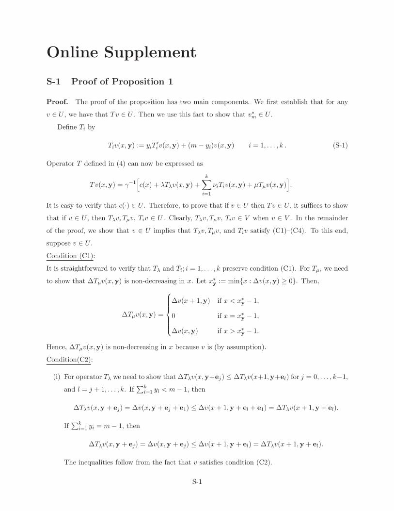
Online Supplement

S-1 Proof of Proposition 1

Proof. The proof of the proposition has two main components. We first establish that for any

v ∈ U , we have that Tv ∈ U . Then we use this fact to show that v∗m ∈ U .

Define Ti by

Tiv(x,y) := yiT′iv(x,y) + (m − yi)v(x,y) i = 1, . . . , k . (S-1)

Operator T defined in (4) can now be expressed as

Tv(x,y) = γ−1[c(x) + λTλv(x,y) +

k∑

i=1

νiTiv(x,y) + µTµv(x,y)].

It is easy to verify that c(·) ∈ U . Therefore, to prove that if v ∈ U then Tv ∈ U , it suffices to show

that if v ∈ U , then Tλv, Tµv, Tiv ∈ U . Clearly, Tλv, Tµv, Tiv ∈ V when v ∈ V . In the remainder

of the proof, we show that v ∈ U implies that Tλv, Tµv, and Tiv satisfy (C1)–(C4). To this end,

suppose v ∈ U .

Condition (C1):

It is straightforward to verify that Tλ and Ti; i = 1, . . . , k preserve condition (C1). For Tµ, we need

to show that ∆Tµv(x,y) is non-decreasing in x. Let x∗y

:= min{x : ∆v(x,y) ≥ 0}. Then,

∆Tµv(x,y) =

∆v(x + 1,y) if x < x∗y− 1,

0 if x = x∗y− 1,

∆v(x,y) if x > x∗y− 1.

Hence, ∆Tµv(x,y) is non-decreasing in x because v is (by assumption).

Condition(C2):

(i) For operator Tλ we need to show that ∆Tλv(x,y+ej) ≤ ∆Tλv(x+1,y+el) for j = 0, . . . , k−1,

and l = j + 1, . . . , k. If∑k

i=1 yi < m − 1, then

∆Tλv(x,y + ej) = ∆v(x,y + ej + e1) ≤ ∆v(x + 1,y + el + e1) = ∆Tλv(x + 1,y + el).

If∑k

i=1 yi = m − 1, then

∆Tλv(x,y + ej) = ∆v(x,y + ej) ≤ ∆v(x + 1,y + el) = ∆Tλv(x + 1,y + el).

The inequalities follow from the fact that v satisfies condition (C2).

S-1

(ii) For operator Ti, we need to show that ∆Tiv(x,y+ej) ≤ ∆Tiv(x+1,y+el) for j = 0, . . . , k−1

and l = j + 1, . . . , k. For i = 1, . . . , k − 1, let J = I{i=j} and L = I{i=l}. When (J,L) ∈

{(0, 0), (0, 1)} the inequalities (S-6) and (S-7) below hold because v satisfies condition (C2).

For (J,L) = (1, 0), the inequalities hold because v satisfies conditions (C2) and (C3).

If yi ≥ 1, we have

∆Tiv(x,y + ej) − ∆Tiv(x + 1,y + el)

= (yi + J)∆v(x,y + ej + ei+1 − ei) + (m − yi − J)∆v(x,y + ej)

−(yi + L)∆v(x + 1,y + el + ei+1 − ei) − (m − yi − L)∆v(x + 1,y + el)

= yi

[∆v(x,y + ej + ei+1 − ei) − ∆v(x + 1,y + el + ei+1 − ei)

](S-2)

+(m − yi − L)[∆v(x,y + ej) − ∆v(x + 1,y + el)

](S-3)

+L[∆v(x,y + ej) − ∆v(x + 1,y + el + ei+1 − ei)

](S-4)

+J[∆v(x,y + ej + ei+1 − ei) − ∆v(x,y + ej)

](S-5)

≤ 0. (S-6)

For additional clarification, observe that if (J,L) = (1, 0), then the term in (S-4) is zero and

we also have i = j and i + 1 = j + 1. So, in (S-5) we have

J[∆v(x,y + ej + ei+1 − ei) − ∆v(x,y + ej)

]= ∆v(x,y + ej+1) − ∆v(x,y + ej).

This expression is non-positive because v is assumed to satisfy condition (C3). The terms in

(S-2) and (S-3) are non-positive because v satisfies condition (C2).

If yi = 0, we have

∆Tiv(x,y + ej) − ∆Tiv(x + 1,y + el)

= J∆v(x,y + ej + J(ei+1 − ei)) + (m − J)∆v(x,y + ej)

−L∆v(x + 1,y + el + L(ei+1 − ei)) − (m − L)∆v(x + 1,y + el)

= (m − L)[∆v(x,y + ej) − ∆v(x + 1,y + el)

]

+L[∆v(x,y + ej) − ∆v(x + 1,y + el + L(ei+1 − ei))

]

+J[∆v(x,y + ej + J(ei+1 − ei)) − ∆v(x,y + ej)

]

≤ 0. (S-7)

Now we consider operator Tk. Let I = I{l=k}. In both cases below (yk ≥ 1 and yk = 0), the

inequalities follow from the fact that v satisfies conditions (C2) and (C3).

S-2

If yk ≥ 1, we have

∆Tkv(x,y + ej) − ∆Tkv(x + 1,y + el)

= yk∆v(x − 1,y + ej − ek) + (m − yk)∆v(x,y + ej)

−(yk + I)∆v(x,y + el − ek) − (m − yk − I)∆v(x + 1,y + el)

= yk

[∆v(x − 1,y + ej − ek) − ∆v(x,y + el − ek)

]

+(m − yk − I)[∆v(x,y + ej) − ∆v(x + 1,y + el)

]

+I[∆v(x,y + ej) − ∆v(x,y + el − ek)

]

≤ 0.

For yk = 0, we have

∆Tkv(x,y + ej) − ∆Tkv(x + 1,y + el)

= m∆v(x,y + ej) − I∆v(x + 1 − I,y + el − Iek) − (m − I)∆v(x + 1,y + el)

= (m − I)[∆v(x,y + ej) − ∆v(x + 1,y + el)

]

+I[∆v(x,y + ej) − ∆v(x + 1 − I,y + el − Iek)

]

≤ 0.

(iii) To verify Tµv satisfies condition (C2), let x∗y+ej

:= min{x : ∆v(x,y + ej) ≥ 0} and x∗y+el

:=

min{x : ∆v(x,y + el) ≥ 0}. By condition (C3) and the definition of x∗y+el

, we have

∆v(x∗y+el

,y + ej) ≥ ∆v(x∗y+el

,y + el) ≥ 0. This implies x∗y+el

≥ x∗y+ej

. Also, by condi-

tion (C2) and the definition of x∗y+ej

, we have ∆v(x∗y+ej

+1,y+el) ≥ ∆v(x∗y+ej

,y+ej) ≥ 0.

This implies x∗y+ej

+ 1 ≥ x∗y+el

. Therefore, x∗y+ej

≤ x∗y+el

≤ x∗y+ej

+ 1 and consequently

x∗y+el

is equal to either x∗y+ej

or x∗y+ej

+ 1.

If x∗y+el

= x∗y+ej

, we distinguish four subcases:

(a) x < x∗y+el

− 2 = x∗y+ej

− 2:

∆Tµv(x + 1,y + el) = ∆v(x + 2,y + el) ≥ ∆v(x + 1,y + ej) = ∆Tµv(x,y + ej).

(b) x = x∗y+el

− 2 = x∗y+ej

− 2:

∆Tµv(x + 1,y + el) = 0 ≥ ∆v(x + 1,y + ej) = ∆Tµv(x,y + ej).

(c) x = x∗y+el

− 1 = x∗y+ej

− 1:

∆Tµv(x + 1,y + el) = ∆v(x + 1,y + el) ≥ 0 = ∆Tµv(x,y + ej).

S-3

(d) x > x∗y+el

− 1 = x∗y+ej

− 1:

∆Tµv(x + 1,y + el) = ∆v(x + 1,y + el) ≥ ∆v(x,y + ej) = ∆Tµv(x,y + ej).

If x∗y+el

= x∗y+ej

+ 1, we distinguish three subcases:

(a) x < x∗y+ej

− 1:

∆Tµv(x + 1,y + el) = ∆v(x + 2,y + el) ≥ ∆v(x + 1,y + ej) = ∆Tµv(x,y + ej).

(b) x = x∗y+el

− 2 = x∗y+ej

− 1:

∆Tµv(x + 1,y + el) = ∆Tµv(x,y + ej) = 0.

(c) x > x∗y+ej

− 1:

∆Tµv(x + 1,y + el) = ∆v(x + 1,y + el) ≥ ∆v(x,y + ej) = ∆Tµv(x,y + ej).

Condition (C3):

(i) For operator Tλ it is straightforward to check that Tλv satisfies condition (C3) when v ∈ U .

(ii) For operator Ti, we need to show that ∆Tiv(x,y+ej+1) ≤ ∆Tiv(x,y+ej) for j = 0, . . . , k−1.

Consider first i = 1, . . . , k − 1, and let J = I{i=j} and K = I{i=j+1}. The three possible

combinations of J and K are (J,K) ∈ {(0, 0), (0, 1), (1, 0)}. The inequalities (S-8) and (S-9)

below follow from the fact that v satisfies condition (C3).

If yi ≥ 1, we have

∆Tiv(x,y + ej+1) − ∆Tiv(x,y + ej)

= (yi + K)∆v(x,y + ej+1 + ei+1 − ei) + (m − yi − K)∆v(x,y + ej+1)

−(yi + J)∆v(x,y + ej + ei+1 − ei) − (m − yi − J)∆v(x,y + ej)

= yi

[∆v(x,y + ej+1 + ei+1 − ei) − ∆v(x,y + ej + ei+1 − ei)

]

+(m − yi − K − J)[∆v(x,y + ej+1) − ∆v(x,y + ej)

]

+K[∆v(x,y + ej+1 + ei+1 − ei) − ∆v(x,y + ej)

]

+J[∆v(x,y + ej+1) − ∆v(x,y + ej + ei+1 − ei)

]

≤ 0. (S-8)

S-4

If yi = 0, we have

∆Tiv(x,y + ej+1) − ∆Tiv(x,y + ej)

= K∆v(x,y + ej+1 + K(ei+1 − ei)) + (m − K)∆v(x,y + ej+1)

−J∆v(x,y + ej + J(ei+1 − ei)) − (m − J)∆v(x,y + ej)

= (m − K − J)[∆v(x,y + ej+1) − ∆v(x,y + ej)

]

+K[∆v(x,y + ej+1 + K(ei+1 − ei)) − ∆v(x,y + ej)

]

+J[∆v(x,y + ej+1) − ∆v(x,y + ej + J(ei+1 − ei))

]

≤ 0. (S-9)

Now we consider operator Tk. Let I = I{j=k−1}. The inequalities (S-10) and (S-11) below

follow from the fact that v satisfies conditions (C2) and (C3).

If yk ≥ 1, we have

∆Tkv(x,y + ej+1) − ∆Tkv(x,y + ej)

= (yk + I)∆v(x − 1,y + ej+1 − ek) + (m − yk − I)∆v(x,y + ej+1)

−yk∆v(x − 1,y + ej − ek) − (m − yk)∆v(x,y + ej)

= yk

[∆v(x − 1,y + ej+1 − ek) − ∆v(x − 1,y + ej − ek)

]

+(m − yk − I)[∆v(x,y + ej+1) − ∆v(x,y + ej)

]

+I[∆v(x − 1,y + ej+1 − ek) − ∆v(x,y + ej)

]

≤ 0. (S-10)

If yk = 0, we have

∆Tkv(x,y + ej+1) − ∆Tkv(x,y + ej)

= I∆v(x − I,y + ej+1 − Iek) + (m − I)∆v(x,y + ej+1) − m∆v(x,y + ej)

= (m − I)[∆v(x,y + ej+1) − ∆v(x,y + ej)

]

+I[∆v(x − I,y + ej+1 − Iek) − ∆v(x,y + ej)

]

≤ 0. (S-11)

(iii) For Tµ, we need to show that ∆Tµv(x,y + ej+1) ≤ ∆Tµv(x,y + ej) for j = 0, . . . , k − 1.

In part (iii) of the argument for condition (C2), we showed that x∗y+ej+1

is either x∗y+ej

or

x∗y+ej

+ 1.

If x∗y+ej+1

= x∗y+ej

, we distinguish three subcases:

S-5

(a) x < x∗y+ej

− 1 :

∆Tµv(x,y + ej+1) = ∆v(x + 1,y + ej+1) ≤ ∆v(x + 1,y + ej) = ∆Tµv(x,y + ej).

(b) x = x∗y+ej

− 1 :

∆Tµv(x,y + ej+1) = ∆Tµv(x,y + ej) = 0.

(c) x > x∗y+ej

− 1 :

∆Tµv(x,y + ej+1) = ∆v(x,y + ej+1) ≤ ∆v(x,y + ej) = ∆Tµv(x,y + ej).

If x∗y+ej+1

= x∗y+ej

+ 1, we distinguish four subcases:

(a) x < x∗y+ej

− 1 :

∆Tµv(x,y + ej+1) = ∆v(x + 1,y + ej+1) ≤ ∆v(x + 1,y + ej) = ∆Tµv(x,y + ej).

(b) x = x∗y+ej

− 1 :

∆Tµv(x,y + ej+1) = ∆v(x + 1,y + ej+1) ≤ 0 = ∆Tµv(x,y + ej).

(c) x = x∗y+ej

:

∆Tµv(x,y + ej+1) = 0 ≤ ∆v(x,y + ej) = ∆Tµv(x,y + ej).

(d) x > x∗y+ej

:

∆Tµv(x,y + ej+1) = ∆v(x,y + ej+1) ≤ ∆v(x,y + ej) = ∆Tµv(x,y + ej).

Condition (C4):

It is easy to verify that if v ∈ U , then Tλv and Tiv; i = 1, . . . , k satisfy condition (C4). For Tµ,

when x < 0, we have:

Tµv(x + 1,y) = min{v(x + 2,y), v(x + 1,y)} ≤ v(x + 1,y) ≤ v(x,y).

Therefore,

Tµv(x + 1,y) ≤ min{v(x + 1,y), v(x,y)} = Tµv(x,y).

This completes the first main component of the proof.

To complete the proof of the proposition, let T 1 = T and define T n = T ◦ T n−1;n > 1. By

Propositions 3.1.5 and 3.1.6 of Bertsekas (2001), v∗m = limn→∞ T nv for any bounded function

S-6

v ∈ V . Take v = v0, where v0 is the function that is identically zero on Sm. It is simple to show

by induction that

0 ≤ T nv0(x,y) ≤b + h

γ

n−1∑

j=0

(|x| + j)αj ,

where α := γ−1(λ+µ+m∑k

i=1 νi) ∈ [0, 1). Hence, we have 0 ≤ v∗m(x,y) = limn→∞ T nv0(x,y) < ∞.

Therefore, v∗m is a real-valued function on Sm (i.e., v∗m ∈ V ).

Note that v0 ∈ U , and so it follows from the argument above that Tv0 ∈ U , and consequently

T nv0 ∈ U for each n. Moreover, it can readily be seen that if functions {vn} and u are such that

vn ∈ U for all n and vn → u ∈ V pointwise, then u ∈ U . We have established that T nv0 ∈ U and

that T nv0 → v∗m ∈ V , and therefore it follows that v∗m ∈ U .

S-2 The Average-Cost Optimality Criteria

Consider the IDD framework of Section 3.1 with m < ∞. A direct analog of Theorem 1 holds for

the average cost criteria. To set the stage, for any policy π ∈ Π, its average-cost is given by

Jπ(x,y) := lim supn→∞

Eπ(x,y)

∑n−1l=0 c(Xl)[τl+1 − τl]

Eπ(x,y)[τn]

= lim supn→∞

Eπ(x,y)

∑n−1l=0 c(Xl)

n.

Let J(x,y) := infπ∈Π Jπ(x,y). A policy that gives average cost J(x,y) for all (x,y) ∈ Sm is said

to be optimal for the average-cost problem.

Theorem S-1 Suppose λ < µ. Then there exists a stationary state-dependent base-stock policy

πA = {πA(x,y)} that is optimal for the average-cost problem. Its base-stock levels {sAy} satisfy the

conditions in (a) and (b) in Theorem 1. In addition, the optimal average cost is finite and indepen-

dent of the initial state; i.e., there is a finite constant J such that J(x,y) = J for all (x,y) ∈ Sm.

Proof. The main idea of the proof is to obtain the desired results for the average-cost problem

by using Proposition 1 for the discounted-cost problem and letting β ↓ 0.

Given a discount rate, let v(x,y) := γv∗m(x,y). The optimality equation (6) can be rewritten

as:

v(x,y) = mina∈{0,1}

{c(x) +

Λ

γ

∑

(x′,y′)∈S

p(x,y),(x′,y′)(a)v(x′,y′)}.

Let α = Λ/γ = Λ/(β + Λ), and define hα(x,y) := vα(x,y) − vα(0, e0), where we have appended a

subscript α to indicate dependence on α (and hence on β).

Parts (i) and (ii) of Theorem 7.2.3 in Sennott (1999) state that under conditions I, II, and III

given below there exists a sequence {αn := Λ/(βn + Λ)} and a real-valued function h(·) such that

S-7

αn ↑ 1 and limn→∞ hαn(x,y) = h(x,y). (Note that αn ↑ 1 means βn ↓ 0.) Moreover, the function

h(·) satisfies

J + h(x,y) ≥ mina∈{0,1}

{c(x) +

∑

(x′,y′)∈S

p(x,y),(x′,y′)(a)h(x′,y′)}

, (S-12)

where J := limα↑1(1 − α)vα(x,y) = limα↑1(1 − α)Λαvα(x,y) is a finite constant. By Theorem

7.2.3(ii), any stationary policy that for each (x,y) selects an action that minimizes the right-hand

side of (S-12) is optimal and yields constant average cost J . Hence, properties of the average-cost

optimal policy are determined through function h(·) in much the same way as were properties of

the discounted-cost optimal policy determined through v∗m(·).

In the following we show that h(·) satisfies conditions (C1)–(C4). For (C1), we need to show

that ∆h(x,y) ≤ ∆h(x + 1,y) for (x,y) ∈ Sm. We have

∆hα(x,y) = ∆vα(x,y) ≤ ∆vα(x + 1,y) = ∆hα(x + 1,y),

so ∆h(x,y) = ∆ limn→∞ hαn(x,y) = limn→∞ ∆hαn(x,y) ≤ limn→∞ ∆hαn(x + 1,y) = ∆ limn→∞

hαn(x+1,y) = ∆h(x+1,y). Similar arguments show that h(·) also satisfies conditions (C2)–(C4).

Hence, as in the proof of Theorem 1, it follows that the policy

πA(x,y) :=

0 if x ≥ sAy

1 if x < sAy

with sAy

:= min{x : h(x + 1,y) − h(x,y) ≥ 0} is optimal for the average-cost problem, and that

properties (a) and (b) described in Theorem 1 hold for {sAy} and πA. For additional background

on the above approach, see Section 8.11 of Puterman (1994).

It remains to show that our problem satisfies conditions that allow application of Theorem 7.2.3.

By Theorem 7.5.6 and Corollary 7.5.9 of Sennott (1999), the following conditions are sufficient to

apply Theorem 7.2.3.

(I) There exists a stationary policy and a state z ∈ Sm such that the induced Markov chain

has a positive recurrent class R ⊆ Sm and the expected first passage time and expected first

passage cost (for definitions see Lemma S-1 below) from any state (x,y) ∈ Sm to z are finite.

(II) For each u > 0, the set {(x,y) ∈ Sm : c(x) ≤ u} is finite.

(III) For each state (x,y) ∈ Sm\R, there exists a policy that induces a Markov chain for which the

expected first passage time and expected first passage cost from state z to (x,y) are finite.

S-8

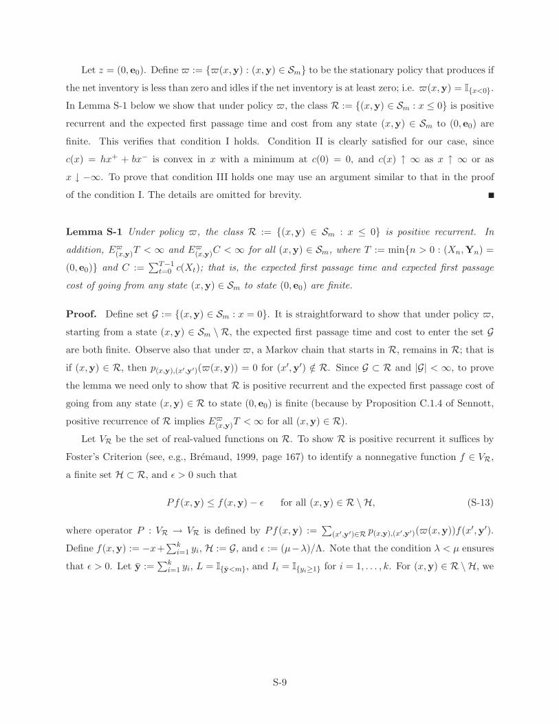
Let z = (0, e0). Define := {(x,y) : (x,y) ∈ Sm} to be the stationary policy that produces if

the net inventory is less than zero and idles if the net inventory is at least zero; i.e. (x,y) = I{x<0}.

In Lemma S-1 below we show that under policy , the class R := {(x,y) ∈ Sm : x ≤ 0} is positive

recurrent and the expected first passage time and cost from any state (x,y) ∈ Sm to (0, e0) are

finite. This verifies that condition I holds. Condition II is clearly satisfied for our case, since

c(x) = hx+ + bx− is convex in x with a minimum at c(0) = 0, and c(x) ↑ ∞ as x ↑ ∞ or as

x ↓ −∞. To prove that condition III holds one may use an argument similar to that in the proof

of the condition I. The details are omitted for brevity.

Lemma S-1 Under policy , the class R := {(x,y) ∈ Sm : x ≤ 0} is positive recurrent. In

addition, E(x,y)T < ∞ and E

(x,y)C < ∞ for all (x,y) ∈ Sm, where T := min{n > 0 : (Xn,Yn) =

(0, e0)} and C :=∑T−1

t=0 c(Xt); that is, the expected first passage time and expected first passage

cost of going from any state (x,y) ∈ Sm to state (0, e0) are finite.

Proof. Define set G := {(x,y) ∈ Sm : x = 0}. It is straightforward to show that under policy ,

starting from a state (x,y) ∈ Sm \ R, the expected first passage time and cost to enter the set G

are both finite. Observe also that under , a Markov chain that starts in R, remains in R; that is

if (x,y) ∈ R, then p(x,y),(x′,y′)((x,y)) = 0 for (x′,y′) /∈ R. Since G ⊂ R and |G| < ∞, to prove

the lemma we need only to show that R is positive recurrent and the expected first passage cost of

going from any state (x,y) ∈ R to state (0, e0) is finite (because by Proposition C.1.4 of Sennott,

positive recurrence of R implies E(x,y)T < ∞ for all (x,y) ∈ R).

Let VR be the set of real-valued functions on R. To show R is positive recurrent it suffices by

Foster’s Criterion (see, e.g., Bremaud, 1999, page 167) to identify a nonnegative function f ∈ VR,

a finite set H ⊂ R, and ǫ > 0 such that

Pf(x,y) ≤ f(x,y) − ǫ for all (x,y) ∈ R \ H, (S-13)

where operator P : VR → VR is defined by Pf(x,y) :=∑

(x′,y′)∈R p(x,y),(x′,y′)((x,y))f(x′,y′).

Define f(x,y) := −x+∑k

i=1 yi, H := G, and ǫ := (µ−λ)/Λ. Note that the condition λ < µ ensures

that ǫ > 0. Let y :=∑k

i=1 yi, L = I{y<m}, and Ii = I{yi≥1} for i = 1, . . . , k. For (x,y) ∈ R \H, we

S-9

have

Pf(x,y) =µ

Λf(x + 1,y) +

λ

Λf(x,y + Le1) +

k−1∑

i=1

νiyi

Λf(x,y + Ii(ei+1 − ei))

+νkyk

Λf(x − Ik,y − Ikek) +

k∑

i=1

νi(m − yi)

Λf(x,y)

≤µ

Λ(−x − 1 + y) +

λ

Λ(−x + y + 1) +

k−1∑

i=1

[νiyi

Λ(−x + y)

]

+νkyk

Λ(−x + y) +

k∑

i=1

[(m − yi)νi

Λ(−x + y)

]

= −x + y −µ

Λ+

λ

Λ

= f(x,y) − ǫ .

Therefore (S-13) holds, and R is positive recurrent. As mentioned above, this also yields E(x,y)T <

∞ for any state (x,y) ∈ R.

Now we show that the expected first passage cost of going from any state (x,y) ∈ R to state

(0, e0) is finite; that is E(x,y)C < ∞. The first step is to show that there exists a nonnegative

function g ∈ VR and a finite set H ⊂ R with (0, e0) ∈ H such that

Pg(x,y) ≤ g(x,y) − c(x) for all (x,y) ∈ R \ H.

Define g(x,y) := θκ−x+y and H := G. For κ > 1, θ > 0, a calculation as above shows that for

(x,y) ∈ R \ H, we have

g(x,y) − Pg(x,y) ≥θ

Λκ−x+y−1

[(λ + µ)κ − µ − λκ2

]. (S-14)

For κ ∈ (1, µ/λ) the term in square brackets in (S-14) is strictly positive. Hence, for such κ and

with θ large enough, the right-hand side of (S-14) exceeds c(x) = hx+ + bx− for all (x,y) ∈ R \H.

The assumption λ < µ ensures that (1, µ/λ) is non-empty. By Corollary C.2.4 of Sennott, the above

proves that E(0,e0)C < ∞. Finally, by Proposition C.2.2(iv) of Sennott it follows that E

(x,y)C < ∞

for any state (x,y) ∈ R. This completes the proof.

S-3 Extension of Theorem 1 to a Random Number of Updates

To extend the model to a setting with a random number of updates, recall that we need to replace

T ′i in (5) by T ′

i given by

T ′iv(x,y) := (1 − qi)T

′iv(x,y) + qiv(x − I{yi≥1},y − eiI{yi≥1}) i = 1, . . . , k

S-10

as defined in (8).

Define operator T by

T v(x,y) :=

k∑

i=1

νi

[yiT

′iv(x,y) + (m − yi)v(x,y)

]

=k∑

i=1

νi

[(1 − qi)Tiv(x,y) + qiT iv(v,y)

](S-15)

where operators {Ti} are defined in (S-1) and operators {T i} are defined by

T iv(x,y) := yiv(x − I{yi≥1},y − eiI{yi≥1}) + (m − yi)v(x,y) i = 1, . . . , k .

The optimality equation for a random number of updates can now be expressed as v = T v where

T is given by

T v(x,y) := γ−1[c(x) + λTλv(x,y) + T v(x,y) + µTµv(x,y)

]. (S-16)

To prove that Theorem 1 holds in the setting with a random number of updates, we need only

prove that T preserves conditions (C1)–(C4). Other steps in the proof carry over without change.

We have seen already (in the proof of Proposition 1) that Tλ, Tµ, and Ti, i = 1, . . . , k preserve

conditions (C1)–(C4). To prove that T preserves conditions (C1)–(C4), it is sufficient [in view of

the preceding fact and (S-15) and (S-16)] to show that T preserves conditions (C1)–(C4) where

Tv(x,y) :=∑k

i=1 νiqiT iv(x,y). Below, we prove this.

It is easy to check that T i preserves conditions (C1) and (C4) for each i = 1, . . . , k. It then

follows that T preserves conditions (C1) and (C4). We next turn to conditions (C2) and (C3).

Condition (C2):

Suppose that v ∈ U . We will prove for each i = 1, . . . , k − 1 that T iv satisfies condition (C2), from

which it follows that Tv satisfies condition (C2). [Note that T k = Tk, where Tk is defined in (S-1).

We already verified that Tk preserves condition (C2) in the proof of Proposition 1.]

Fix i ∈ {0, . . . , k − 1}, j ∈ {0, . . . , k − 1}, and l ∈ {j + 1, . . . , k}. Let J = I{i=j} and L = I{i=l}.

We will prove that ∆T iv(x,y + ej) ≤ ∆T i(x + 1,y + el).

S-11

Suppose first that yi ≥ 1. Then we have

∆T iv(x,y + ej) − ∆T iv(x + 1,y + el)

= (yi + J)∆v(x − 1,y + ej − ei) + (m − yi − J)∆v(x,y + ej)

−(yi + L)∆v(x,y + el − ei) − (m − yi − L)∆v(x + 1,y + el)

= yi

[∆v(x − 1,y + ej − ei) − ∆v(x,y + el − ei)

]

+(m − yi − L)[∆v(x,y + ej) − ∆v(x + 1,y + el)

]

+L[∆v(x,y + ej) − ∆v(x,y + el − ei)

]

+J[∆v(x − 1,y + ej − ei) − ∆v(x,y + ej)

]

≤ 0,

where the inequality follows by considering each of the three possibilities (J,L) = (0, 0), (0, 1), (1, 0)

separately and using the fact that v is assumed to satisfy conditions (C2) and (C3).

Suppose next that yi = 0. Then

∆T iv(x,y + ej) − ∆T iv(x + 1,y + el)

= J∆v(x − J,y + ej − Jej) + (m − J)∆v(x,y + ej)

−L∆v(x + 1 − L,y + el − Lel) − (m − L)∆v(x + 1,y + el)

= (m − L)[∆v(x,y + ej) − ∆v(x + 1,y + el)

]

+L[∆v(x,y + ej) − ∆v(x + 1 − L,y + el − Lel)

]

+J[∆v(x − J,y + ej − Jej) − ∆v(x,y + ej)

]

≤ 0.

where again the inequality follows by considering each of the three possibilities for (J,L) separately

and using the fact that v satisfies conditions (C2) and (C3).

Condition (C3)

Suppose again that v ∈ U . It turns out that it may be that T iv does not satisfy condition (C3).

So, we will show directly that Tv satisfies condition (C3), rather than trying to work with the

individual {T i}. This will complete the proof that if v ∈ U , then Tv ∈ U .

Fix j ∈ {0, . . . , k − 1}. We want to show that ∆Tv(x,y + ej+1) ≤ ∆Tv(x,y + ej). For each

i = 1, . . . , k let Ji = I{i=j}, and Ki = I{i=j+1}.

S-12

For i = 1, . . . , k, if yi ≥ 1 then

∆T iv(x,y + ej+1) − ∆T iv(x,y + ej)

= (yi + Ki)∆v(x − 1,y + ej+1 − ei) + (m − yi − Ki)∆v(x,y + ej+1)

− (yi + Ji)∆v(x − 1,y + ej − ei) − (m − yi − Ji)∆v(x,y + ej)

= yi

[∆v(x − 1,y + ej+1 − ei) − ∆v(x − 1,y + ej − ei)

]

+ (m − yi − Ki)[∆v(x,y + ej+1) − ∆v(x,y + ej)

]

+ Ki

[∆v(x − 1,y + ej+1 − ei) − ∆v(x,y + ej)

]

+ Ji

[∆v(x,y + ej) − ∆v(x − 1,y + ej − ei)

]

and if yi = 0 then

∆T iv(x,y + ej+1) − ∆T iv(x,y + ej)

= (yi + Ki)∆v(x − Ki,y + ej+1 − Kiei) + (m − yi − Ki)∆v(x,y + ej+1)

− (yi + Ji)∆v(x − Ji,y + ej − Jiei) − (m − yi − Ji)∆v(x,y + ej)

= yi

[∆v(x − 1,y + ej+1 − Kiei) − ∆v(x − 1,y + ej − Jiei)

]

+ (m − yi − Ki)[∆v(x,y + ej+1) − ∆v(x,y + ej)

]

+ Ki

[∆v(x − 1,y + ej+1 − Kiei) − ∆v(x,y + ej)

]

+ Ji

[∆v(x,y + ej) − ∆v(x − 1,y + ej − Jiei)

].

Therefore,

∆Tv(x,y + ej+1) − ∆Tv(x,y + ej) =

k∑

i=1

νiqi

[∆T iv(x,y + ej+1) − ∆T iv(x,y + ej)

]

=

k∑

i=1

Ai +

k∑

i=1

Bi +

k∑

i=1

Ci +

k∑

i=1

Di (S-17)

S-13

where

Ai =

νiqiyi

[∆v(x − 1,y + ej+1 − ei) − ∆v(x − 1,y + ej − ei)

]if yi ≥ 1

0 if yi = 0

Bi = νiqi(m − yi − Ki)[∆v(x,y + ej+1) − ∆v(x,y + ej)

]

Ci =

νiqiKi

[∆v(x − 1,y + ej+1 − ei) − ∆v(x,y + ej)

]if yi ≥ 1

νiqiKi

[∆v(x − Ki,y + ej+1 − Kiei) − ∆v(x,y + ej)

]if yi = 0

Di =

νiqiJi

[∆v(x,y + ej) − ∆v(x − 1,y + ej − ei)

]if yi ≥ 1

νiqiJi

[∆v(x,y + ej) − ∆v(x − Ji,y + ej − Jiei)

]if yi = 0 .

We have that Ai ≤ 0 and Bi ≤ 0 for all i = 1, . . . , k because v satisfies condition (C3). If

j 6= 0, then the only non-zero terms in the third and fourth summations in (S-17) are Cj+1 and

Dj . Therefore,

k∑

i=1

Ci +k∑

i=1

Di = νj+1qj+1

[∆v(x − 1,y) − ∆v(x,y + ej)

]+ νjqj

[∆v(x,y + ej) − ∆v(x − 1,y)

]

= (νj+1qj+1 − νjqj)[∆v(x − 1,y) − ∆v(x,y + ej)

]

Recall that v satisfies condition (C2), and therefore ∆v(x − 1,y) − ∆v(x,y + ej) ≤ 0. When

νj+1qj ≥ νjqj, we have that∑k

i=1 Ci +∑k

i=1 Di ≤ 0. Note that this is the only place where we have

used the condition that νiqi is non-decreasing in i. We have now shown that ∆Tv(x,y + ej+1) −

∆Tv(x,y + ej) =∑k

i=1 Ai +∑k

i=1 Bi +∑k

i=1 Ci +∑k

i=1 Di ≤ 0, as desired.

If j = 0, then∑k

i=1 Ci +∑k

i=1 Di = ν1q1[∆v(x − 1,y) − ∆v(x,y)] ≤ 0, where the inequality

holds because v satisfies condition (C1). Again, we have ∆Tv(x,y + ej+1) − ∆Tv(x,y + ej) ≤ 0,

which completes the argument.

S-4 Extension of Theorem 1 to Systems with Cancelations

In this section we re-define some of the notation used in the preceding section.

Let {T i} be defined by

T iv(x,y) := yiv(x,y − eiI{yi≥1}) + (m − yi)v(x,y) i = 1, . . . , k

and let T be defined by

Tv(x,y) :=

k∑

i=1

νipiT iv(x,y) .

S-14

By an argument identical to that at the beginning of Section S-3, to extend Theorem 1 to the

setting with cancelations, we need only prove that T preserves conditions (C1)–(C4). That is, we

just need to show that if v ∈ U , then Tv ∈ U .

Suppose that v satisfies conditions (C1)–(C4); that is, suppose v ∈ U . It can be easily seen that

T iv satisfies conditions (C1) and (C4) from which it follows that Tv satisfies conditions (C1) and

(C4). We next check that Tv satisfies conditions (C2) and (C3).

Condition (C2): Suppose i ∈ {1, . . . , k}, j ∈ {0, . . . , k − 1}, and l ∈ {j + 1, . . . , k}. Let J = I{i=j}

and L = I{i=l}. Note that if i = k, then J = 0. If yi ≥ 1 we have

∆T iv(x,y + ej) − ∆T iv(x + 1,y + el)

= (yi + J)∆v(x,y + ej − ei) + (m − yi − J)∆v(x,y + ej)

−(yi + L)∆v(x + 1,y + el − ei) − (m − yi − L)∆v(x + 1,y + el)

= yi

[∆v(x,y + ej − ei) − ∆v(x + 1,y + el − ei)

]

+(m − yi − J)[∆v(x,y + ej) − ∆v(x + 1,y + el)

]

+L[∆v(x + 1,y + el) − ∆v(x + 1,y + el − ei)

]

+J[∆v(x,y + ej − ei) − ∆v(x + 1,y + el)

]

≤ 0.

If yi = 0, we have

∆T iv(x,y + ej) − ∆T iv(x + 1,y + el)

= J∆v(x,y + ej − Jei) + (m − J)∆v(x,y + ej)

−L∆v(x + 1,y + el − Lei) − (m − L)∆v(x + 1,y + el)

= (m − J)[∆v(x,y + ej) − ∆v(x + 1,y + el)

]

+L[∆v(x + 1,y + el) − ∆v(x + 1,y + el − Lei)

]

+J[∆v(x,y + ej − Jei) − ∆v(x + 1,y + el)

]

≤ 0.

We have proved that each T iv satisfies condition (C2), and therefore Tv satisfies condition (C2).

Condition (C3): Suppose j ∈ {0, . . . , k − 1}. For i = 1, . . . , k, let Ji = I{i=j} and Ki = I{i=j+1}.

S-15

For i = 1, . . . , k, if yi ≥ 1 we have

∆T iv(x,y + ej+1) − ∆T iv(x,y + ej)

= (yi + Ki)∆v(x,y + ej+1 − ei) + (m − yi − Ki)∆v(x,y + ej+1)

−(yi + Ji)∆v(x,y + ej − ei) − (m − yi − Ji)∆v(x,y + ej)

= yi

[∆v(x,y + ej+1 − ei) − ∆v(x,y + ej − ei)

]

+(m − yi − Ki)[∆v(x,y + ej+1) − ∆v(x,y + ej)

]

+Ki

[∆v(x,y + ej+1 − ei) − ∆v(x,y + ej)

]

+Ji

[∆v(x,y + ej) − ∆v(x,y + ej − ei)

]

and if yi = 0 we have

∆T iv(x,y + ej+1) − ∆T iv(x,y + ej)

= (yi + Ki)∆v(x,y + ej+1 − Kiei) + (m − yi − Ki)∆v(x,y + ej+1)

−(yi + Ji)∆v(x,y + ej − Jiei) − (m − yi − Ji)∆v(x,y + ej)

= yi

[∆v(x,y + ej+1 − Kiei) − ∆v(x,y + ej − Jiei)

]

+(m − yi − Ki)[∆v(x,y + ej+1) − ∆v(x,y + ej)

]

+Ki

[∆v(x,y + ej+1 − Kiei) − ∆v(x,y + ej)

]

+Ji

[∆v(x,y + ej) − ∆v(x,y + ej − Jiei)

].

Therefore,

∆Tv(x,y + ej+1) − ∆Tv(x,y + ej) =

k∑

i=1

νipi

[∆T iv(x,y + ej+1) − ∆T iv(x,y + ej)

]

=k∑

i=1

Ai +k∑

i=1

Bi +k∑

i=1

Ci +k∑

i=1

Di (S-18)

where

Ai = νipiyi

[∆v(x,y + ej+1 − ei) − ∆v(x,y + ej − ei)

]

Bi = νipi(m − yi − Ki)[∆v(x,y + ej+1) − ∆v(x,y + ej)

]

Ci = νipiKi

[∆v(x,y + ej+1 − ei) − ∆v(x,y + ej)

]

Di = νipiJi

[∆v(x,y + ej) − ∆v(x,y + ej − ei)

]

Note that the preceding expressions combine the yi ≥ 0 and yi = 0 cases.

S-16

We have that Ai ≤ 0 and Bi ≤ 0 for all i = 1, . . . , k because v satisfies condition (C3). If

j 6= 0, then the only non-zero terms in the third and fourth summations in (S-18) are Cj+1 and

Dj . Therefore,

k∑

i=1

Ci +k∑

i=1

Di = νj+1pj+1

[∆v(x,y) − ∆v(x,y + ej)

]+ νjpj

[∆v(x,y + ej) − ∆v(x,y)

]

= (νj+1pj+1 − νjpj)[∆v(x,y) − ∆v(x,y + ej)

].

We have assumed that v satisfies condition (C3), from which we have ∆v(x,y)−∆v(x,y+ej) ≥ 0.

Hence, if νj+1pj+1 ≤ νjpj , then∑k

i=1 Ci +∑k

i=1 Di ≤ 0. If j = 0, then∑k

i=1 Ci +∑k

i=1 Di = 0.

Thus, we have proved that Tv satisfies condition (C3), which completes the argument.

S-5 Extension of Theorem 1 to Systems with Lost Sales

To model lost sales, in (5) we replace operator T ′k by T ′

k defined in (9), and we re-define the state

space to be Z+×Zk+(m) and the cost function to be c(x) = hx. Similar to the proof of Proposition 1,

the operator T in the optimality equation can be written as

Tv(x,y) = γ−1[c(x) + λTλv(x,y) +

k−1∑

i=1

νiTiv(x,y) + νkTkv(x,y) + µTµv(x,y)]

(S-19)

where {Ti : i = 1, . . . , k − 1} are defined in (S-1) and Tk is defined by

Tkv(x,y) :=yiT′kv(x,y) + (m − yk)v(x,y)

=yi

[v([x − I{yk≥1}]

+,y − ekI{yk≥1}) + cLSI{yk≥1 and x=0}

]+ (m − yk)v(x,y) .

To prove that Theorem 1 [except property (b), which deals with backorders] holds in this

setting, we shall just need to show that the value function satisfies conditions (C1)–(C3). Note

that condition (C4) is not relevant in the setting with lost sales. To prove the desired result, we

introduce the following additional condition:

(C4)′ ∆v(x,y) ≥ −cLS for all x ≥ 0, y ∈ Zk+(m).

We will next show that if function v satisfies conditions (C1)–(C3) and (C4)′, then Tv satisfies

conditions (C1)–(C3) and (C4)′. That is, we will show that operator T in (S-19) preserves condi-

tions (C1)–(C3) and (C4)′. As in the proof of Proposition 1, it then follows that the value function

satisfies the conditions (C1)–(C3). It also follows that the value function satisfies condition (C4)′,

but this fact is not needed for the theorem.

Suppose that v satisfies conditions (C1)–(C3) and (C4)′.

S-17

From the proof of Proposition 1, we have that Tλv, {Tiv : i = 1, . . . , k − 1}, and Tµv satisfy

conditions (C1)–(C3). We next show that Tkv satisfies conditions (C1)–(C3). Note that Tkv(x,y) =

Tkv(x,y) when x > 0 or yk = 0, where Tk is defined in (S-1). Hence, the inequalities in conditions

(C1)–(C3) hold when x > 0 or yk = 0; this was shown in the proof of Proposition 1. Therefore, to

show that Tkv satisfies conditions (C1)–(C3), we need only show that the inequalities hold when

x = 0 and yk ≥ 1. That is, we just need to show that

∆Tkv(0,y) ≤ ∆Tk(1,y) for all y ∈ Zk+(m) with yk ≥ 1 (S-20)

∆Tkv(0,y + ej) ≤ ∆Tkv(1,y + el) for all y ∈ Zk+(m − 1) with yk ≥ 1, j = 0, . . . , k − 1, and l = j + 1, . . . , k

(S-21)

∆Tkv(0,y + ej+1) ≤ ∆Tkv(0,y + ej) for all y ∈ Zk+(m − 1) with yk ≥ 1, and j = 0, . . . , k − 1.

(S-22)

To check that (S-20) holds, suppose that y is such that yk ≥ 1. We have

∆Tkv(0,y) − ∆Tkv(1,y) = (m − yk)∆v(0,y) − ykcLS − yk∆v(0,y − ek) − (m − yk)∆v(1,y)

= (m − yk)[∆v(0,y) − ∆v(1,y)

]− yk

[cLS + ∆v(0,y − ek)

]

≤ 0

where the inequality holds because v satisfies conditions (C1) and (C4)′. Hence, (S-20) holds. Next

we check that (S-21) holds. Fix j ∈ {0, . . . , k − 1} and l ∈ {j + 1, . . . , k} and let I = I{l=k}. Then

∆Tkv(0,y + ej) − ∆Tkv(1,y + el) = (m − yk)∆v(0,y + ej) − ykcLS

− (yk + I)∆v(0,y + el − ek) − (m − yk − I)∆v(1,y + el)

= (m − yk − I)[∆v(0,y + ej) − ∆v(1,y + el)

]

− yk

[cLS + ∆v(0,y + el − ek)

]

+ I[∆v(0,y + ej) − ∆v(0,y + el − ek)

]

≤ 0,

where the inequality holds because v satisfies conditions (C2), (C3), and (C4)′. Finally, we verify

S-18

that (S-21) holds:

∆Tkv(0,y + ej+1) − ∆Tkv(0,y + ej) = (m − yk − I)∆v(0,y + ej+1) − (yk + I)cLS

− (m − yk)∆v(0,y + ej) + ykcLS

= (m − yk − I)[∆v(0,y + ej+1) − ∆v(0,y + ej)

]

− I[cLS + ∆v(0,y + ej)

]

≤ 0,

because v satisfies conditions (C3) and (C4)′. We have now shown that Tkv satisfies conditions (C1)–

(C3) and therefore Tv satisfies (C1)–(C3).

To complete the proof of the extension of Theorem 1, we next show that Tv satisfies condi-

tion (C4)′. This follows easily from (S-19) and the fact that γ = β + λ + µ + m∑k

i=1 νi.

S-6 Additional Material for Section 3.2

In this section we describe results of GH (Guo and Hernandez-Lerma 2003), and show how they

may be applied in our setting. GH consider continuous time MDPs with countable state space S

and discount rate β. The set of allowable actions in state i ∈ S is A(i). The conditional transition

rate from state i ∈ S to state j 6= i under action a ∈ A(i) is given by q(j|i, a) where q(j|i, a) ≥ 0

for i 6= j. Let q(i) := supa∈A(i) qi(a) < ∞ where qi(a) := −q(i|i, a) :=∑

j 6=i q(j|i, a). The reward

rate is r(i, a) in state i ∈ S under action a ∈ A(i).

To put our model into their framework, take S = S, β = β, A(i) = {0, 1}, r((x,y), a) = −c(x)

and for (x′,y′) 6= (x,y) take

q((x′,y′)|(x,y), a) =

µI{a=1} if (x′,y′) = (x + 1,y)

λ if (x′,y′) = (x,y + e1)

νiyi if (x′,y′) = (x,y + ei+1 − ei) i = 1, . . . , k − 1

νkyk if (x′,y′) = (x − 1,y − ek)

0 otherwise.

With the above, we have q(x,y)(a) = −q((x,y)|(x,y), a) = λ +∑k

i=1 νiyi + µI{a=1}, and q(x,y) =

λ +∑k

i=1 νiyi + µ. GH introduce the following assumptions.

Assumption A. There exist a sequence {Sm : m ≥ 1} of subsets of S, a non-negative function R

on S and constants b ≥ 0 and c0 ∈ (−∞,∞) such that

S-19

(1) Sm ↑ S and supi∈Smq(i) < ∞ for each m ≥ 1;

(2) limm→∞[infj /∈SmR(j)] = +∞; and

(3)∑

j∈S q(j|i, a)R(j) ≤ c0R(i) + b for all i ∈ S and a ∈ A(i).

Assumption B. With c0 and R as in Assumption A:

(1) either c0 ≤ 0 or c0 − β < 0 when c > 0; and

(2) there exist non-negative constants M1 and M2 such that |r(i, a)| ≤ M1 + M2R(i) for all i ∈

S and a ∈ A(i) .

Assumption C.

(1) For each i ∈ S, A(i) is compact;

(2) the functions r(i, a), q(i|j, a) and∑

j∈S q(j|i, a)R(j) are continuous in a ∈ A(i) for each fixed

i, j ∈ S; and

(3) there exist a non-negative function w′ on S and constants c′ > 0, b′ > 0, and M ′ > 0 such

that q(i)R(i) ≤ M ′w′(i) and∑

j∈S q(j|i, a)w′(j) ≤ c′w′(i) + b′ for all (i, a).

Parts (b) and (c) of Theorem 3.2 of GH state that if Assumptions A and B hold, then the value

function v∗ is the unique solution in BR(S) := {v : there exist constants c1, c2 ≥ 0 so that |v(i)| ≤

c1 + c2R(i) for all i ∈ S} of the optimality equation,

v(i) =1

β + q(i)sup

{r(i, a) +

∑

j 6=i

q(j|i, a)v(j) + [q(i) − qi(a)]v(i)}

i ∈ S . (S-23)

Part (e) of Theorem 3.2 states that if, in addition, Assumption C holds, then there exists an optimal

stationary policy. When Assumptions A, B, and C(3) hold, then Theorem 3.3 of GH states that if

{a∗(i)} satisfy

v∗(i) =1

β + q(i)

{r(i, a∗(i)) +

∑

j 6=i

q(j|i, a∗(i))v∗(j) +[q(i) − qi(a

∗(i))]v∗(i)

}i ∈ S , (S-24)

then {a∗(i)} is an optimal (stationary) policy.

Before we proceed, observe that the equation v = Lv in Section 3.2 is simply (S-23) specialized

to our context, and multiplied by −1 to express our cost minimization as a (negative) revenue

maximization.

Lemma S-2 The system with IDD and unbounded jump rates satisfies Assumptions A, B, and C

of GH.

S-20

Proof. Let R(x,y) := |x| +∑k

i=1 yi = |x| + y be as defined in (10) and let Sm = Sm. Then

Assumptions A(1) and A(2) hold trivially. For A(3) and B(1) we need to identify constants c0 ≤ 0

and b ≥ 0 so that

λR(x,y + e1) +

k−1∑

i=1

νiyiR(x,y + ei+1 − ei) + νkykR(x − 1,y − ek) + µI{a=1}R(x + 1,y)

− [λ +k∑

i=1

νiyi + µI{a=1}]R(x,y) ≤ c0R(x,y) + b (S-25)

for all (x,y) ∈ S and a ∈ {0, 1}. The expression on the left side above simplifies to λ[R(x,y +

e1)−R(x,y)] + νkyk[R(x− 1,y− ek)−R(x,y)] + µI{a=1}[R(x + 1,y)−R(x,y)], which is bounded

above by λ + µ. Hence (S-25) holds with c0 = 0 and b = λ + µ. Thus, Conditions A(3) and B(1)

hold. For B(2) we need constants M1,M2 ≥ 0 so that c(x) ≤ M1 + M2R(x,y), for all (x,y) ∈ S.

It is easy to see that B(2) holds with M1 = 0 and M2 = b + h.

The compactness and continuity Assumptions C(1) and C(2) hold trivially because our action

space is finite. For C(3), we need to identify a non-negative function w′ : S → S and constants

b′ ≥ 0, c′ > 0, and M ′ > 0 such that

(λ +k∑

i=1

νiyi + µ)R(x,y) ≤ M ′w′(x,y) for all (x,y) ∈ S (S-26)

and

λw′(x,y + e1) +

k−1∑

i=1

νiyiw′(x,y + ei+1 − ei) + νkykw

′(x − 1,y − ek) + µI{a=1}w′(x + 1,y)

− [λ +

k∑

i=1

νiyi + µI{a=1}]w′(x,y) ≤ c′w′(x,y) + b′ (S-27)

Let w′(x,y) := (|x| + y)2 and M ′ := λ + µ + max{ν1, . . . , νk}. Note that (S-26) holds when

x = y = 0. Otherwise, we have either |x| ≥ 1 or y ≥ 1 (or both), and hence

λ +k∑

i=1

νiyi + µ ≤ M ′(|x| + y) .

S-21

Multiplying the above by R(x,y) yields (S-26). The left-hand side of (S-27) simplifies to

λ[w′(x,y + e1) − w′(x,y)] + νkyk[w′(x − 1,y − ek) − w′(x,y)]

+ µI{a=1}[w′(x + 1,y) − w′(x,y)]

≤ λ[w′(x,y + e1) − w′(x,y)] + µ[w′(x + 1,y) − w′(x,y)]

≤ 2λ(|x| + y) + λ + 2µ(|x| + y) + µ

= 2(λ + µ)(|x| + y) + (λ + µ)

≤ 2(λ + µ)w′(x,y) + (λ + µ).

Therefore, C(3) holds with c′ := 2(λ + µ) and b′ := λ + µ. This completes the proof.

S-7 Systems with IDD and Low Arrival Rate

For small enough λ, a system with no ADI will hold no inventory and produce to order, giving an

average cost of approximately C1 := λb/µ; this expression comes from ignoring the possibility of

multiple orders being present at once (which is not unreasonable when λ is very small) and noting

that jobs arrive at rate λ and incur cost at rate b during the time it takes to produce one unit,

which has mean 1/µ. For a system with ADI, it will again be best not to hold inventory when no

jobs are in the demand leadtime system. When an order is announced, then the decision is whether

or not to produce one unit in advance of the order be coming due. Again ignoring the possibility of

multiple orders being present simultaneously, if the decision is not to produce upon announcement

of an order, then the long-run average cost will again be roughly C1 = λb/µ. If the decision is to

commence production upon announcement of an order, then we can derive an approximation for the

average cost by conditioning on whether the production is completed prior to the order becoming

due [which occurs with probability µ/(µ + ν)] or not [which occurs with probability ν/(µ + ν)].

By standard properties of exponential random variables, the order will generate an average holding

cost of h/ν conditional upon the unit completing production prior to the order becoming due.

Similarly, the order will generate an average backorder cost of b/µ conditional upon the unit not

completing production prior to the order coming due. Putting it together, the long-run average

cost is approximately C2 := λ[ µµ+ν

hν + ν

µ+νbµ ].

Hence, for the system with ADI, it will be better to produce upon announcement of an order

provided C2 < C1. Rearranging terms, it follows that it is better to produce if ν > ν∗(µ) := hµ/b

and it is better to wait for the order to become due otherwise. It follows that if ν > ν∗(µ) then

PCR = 100 × (JN − JA)/JN ≈ 100 × (C1 − C2)/C1 = 100 × (bµν − hµ2)/(bµν + bν2) for λ small.

S-22

Likewise, if ν ≤ ν∗(µ) then PCR ≈ 0 for λ small. A similar analysis is possible for general k.

S-8 Extra Material for Section 5

Proof of Theorem 3. To prove (a), note that by Proposition S-1, the value function v∗ satisfies

conditions (C2) and (C3). Applying Condition (C3) and using the definition of sy+erw , we have

∆v∗(sy+erw ,y + epq) ≥ ∆v∗(sy+erw ,y + erw) ≥ 0, which implies sy+erw ≥ sy+epq . Also, by

Condition (C2) and the definition of sy+epq , we have ∆v∗(sy+epq + 1,y + erw) ≥ ∆v∗(sy+epq ,y +

epq) ≥ 0, which implies sy+epq + 1 ≥ sy+erw . Therefore, sy+epq ≤ sy+erw ≤ sy+epq + 1 and hence

sy+erw is equal to either sy+epq or sy+epq + 1. Finally, part (b) is a consequence of the fact that v∗

satisfies Condition (C4).

Proposition S-1 The value function v∗ satisfies Conditions (C1)–(C5).

Proof. If T preserves Conditions (C1)–(C5), then it will follow by an argument identical to that

at the end of the proof of Proposition 1 that v∗ satisfies Conditions (C1)–(C5). Hence, we need

only prove that if v ∈ V satisfies Conditions (C1)–(C5), then so does T v.

To this end, suppose hereafter that v satisfies Conditions (C1)–(C5).

We will check that T v satisfies Conditions (C1)–(C5). As before, it is sufficient to verify that

each of {Tijv} and Tµv individually satisfies the five conditions. For Conditions (C1) and (C4)

the verification is essentially identical to the approach used for Conditions C1 and C4 in the proof

of Proposition 1; hence we omit the details. Likewise, the verification that Tµv satisfies the five

conditions is virtually identical to the corresponding arguments in Proposition 1. Hence, we present

only a few comments where there are minor differences in the verification for Tµv.

We begin by checking Conditions (C2) and (C3). For this, suppose (p, q) ≺ (r, w), and y +

epq,y + erw ∈ Y, and let Jij = I{(p,q)=(i,j)} and Lij = I{(r,w)=(i,j)}.

To verify that Tµv satisfies Conditions (C2) and (C3), let x∗(y) := min{x : ∆v(x,y + epq) ≥ 0}

for y ∈ Y. Similar to IDD systems, we have that x∗y+erw

is either x∗y+epq

or x∗y+epq

+ 1, because v

satisfies Conditions (C2) and (C3). Proof that Tµv does indeed satisfy Conditions (C2) and (C3)

follows by considering cases directly analogous to those used for Tµ in the proof of Proposition 1.

Condition (C2): For operators {Tij}, we need to show that ∆Tijv(x,y+epq) ≤ ∆Tijv(x+1,y+erw).

(a) For i = 0, j = 1, . . . , k0 − 1, the operator Tij = T0j is given by (12).

S-23

If y0j = 1 then

∆T0jv(x,y + epq) = ∆v(x,y + epq + e0,j+1 − e0j)

≤ ∆v(x + 1,y + erw + e0,j+1 − e0j)

= ∆T0jv(x + 1,y + erw) ,

where the inequality holds because v is assumed to satisfy Condition (C2).

If y0j 6= 1 then

∆T0jv(x,y + epq) = ∆v(x,y + epq + J0j(e0,j+1 − e0j))

≤ ∆v(x + 1,y + erw + L0j(e0,j+1 − e0j))

= ∆T0jv(x + 1,y + erw) .

The inequality above can be checked by looking at the three possible values of (J0j , L0j). If

(J0j , L0j) ∈ {(0, 0), (1, 0), (0, 1)}, the inequality holds because v satisfies Condition (C2).

(b) For i = 0, j = k0, the operator Tij = T0k0is given by (13). Let I1 = I{n=0}.

If y0k0= 1 then

∆T0k0v(x,y + epq) = ∆v(x − I1,y + epq + e01 − e0k0

+ (1 − I1)e11)

≤ ∆v(x + 1 − I1,y + erw + e01 − e0k0+ (1 − I1)e11)

= ∆T0k0v(x + 1,y + erw) .

If y0k06= 1

∆T0k0v(x,y + epq) = ∆v(x − J0k0

I1,y + epq + J0k0(e01 − e0k0

+ (1 − I1)e11))

≤ ∆v(x + 1 − L0k0I1,y + erw + L0k0

(e01 − e0k0+ (1 − I1)e11))

= ∆T0k0v(x + 1,y + erw) .

The inequalities above follow from the fact that v satisfies Conditions (C2)–(C3).

(c) For i = 1, . . . , n, j = 1 the operator Tij = Ti1 is given by (14) when ki ≥ 2. Let I2 =

I{(p,q)6=(i,l) for l=2,...,ki} and I3 = I{(r,w)6=(i,l) for l=2,...,ki}.

If yi1 ≥ 1 and yil = 0 for l = 2, . . . , ki then

∆Ti1v(x,y + epq) = ∆v(x,y + epq + I2(ei2 − ei1))

≤ ∆v(x + 1,y + erw + I3(ei2 − ei1))

= ∆Ti1v(x + 1,y + erw).

S-24

If yi1 = 0 and yil = 0 for l = 2, . . . , ki

∆Ti1v(x,y + epq) = ∆v(x,y + epq + Ji1(ei2 − ei1))

≤ ∆v(x + 1,y + erw + Li1(ei2 − ei1))

= ∆Ti1v(x + 1,y + erw).

If yil ≥ 1 for some l = 2, . . . , ki then

∆Ti1v(x,y + epq) = ∆v(x,y + epq)

≤ ∆v(x + 1,y + erw)

= ∆Ti1v(x + 1,y + erw).

The inequalities above follow from the fact that v satisfies Conditions (C1)–(C3).

(d) For i = 1, . . . , n, j = 2, . . . , ki − 1, the operator Tij is given by (15).

If yij = 1

∆Tijv(x,y + epq) = ∆v(x,y + epq + ei,j+1 − eij)

≤ ∆v(x + 1,y + erw + ei,j+1 − eij)

= ∆Tijv(x + 1,y + erw).

If yij = 0

∆Tijv(x,y + epq) = ∆v(x,y + epq + Jij(ei,j+1 − eij))

≤ ∆v(x + 1,y + erw + Lij(ei,j+1 − eij))

= ∆Tijv(x + 1,y + erw).

The inequalities above follow from the fact that v satisfies Conditions (C1) and (C2).

(e) For i = 1, . . . , n and j = ki, the operator Tikiis given by (16) and (17) . Let I4 = I{i=n}.

Using the fact that v satisfies Conditions (C1)–(C3) we have the following.

If yiki≥ 1 then

∆Tikiv(x,y + epq) = ∆v(x − I4,y + epq − eiki

+ (1 − I4)ei+1,1)

≤ ∆v(x + 1 − I4,y + erw − eiki+ (1 − I4)ei+1,1)

= Tikiv(x + 1,y + erw) .

S-25

If yiki= 0 then

∆Tikiv(x,y + epq) = ∆v(x − Jiki

I4,y + epq + Jiki(−eiki

+ (1 − I4)ei+1,1))

≤ ∆v(x + 1 − LikiI4,y + erw + Liki

(−eiki+ (1 − I4)ei+1,1))

= Tikiv(x + 1,y + erw).

This completes the verification that each Tijv satisfies Condition (C2).

Condition (C3): For operators {Tij}, we need to show that ∆Tijv(x,y + erw) ≤ ∆Tijv(x,y + epq).

(a) For i = 0, j = 1, . . . , k0 − 1, the operator Tij = T0j is given by (12).

If y0j = 1 then

∆T0jv(x,y + erw) = ∆v(x,y + erw + e0,j+1 − e0j)

≤ ∆v(x,y + epq + e0,j+1 − e0j)

= ∆T0jv(x + 1,y + epq).

If y0j 6= 1 then

∆T0jv(x,y + erw) = ∆v(x,y + erw + L0j(e0,j+1 − e0j))

≤ ∆v(x,y + epq + J0j(e0,j+1 − e0j))

= ∆T0jv(x,y + epq).

The inequalities above follow the fact that v satisfies condition (C3).

(b) For i = 0, j = k0, the operator Tij = T0k0is given by (13). Let I1 = I{n=0}.

If y0k0= 1 then

∆T0k0v(x,y + erw) = ∆v(x − I1,y + erw + e01 − e0k0

+ (1 − I1)e11)

≤ ∆v(x − I1,y + epq + e01 − e0k0+ (1 − I1)e11)

= ∆T0k0v(x,y + epq).

If y0k06= 1 then

∆T0k0v(x,y + erw) = ∆v(x − L0k0

I1,y + erw + L0k0(e01 − e0k0

+ (1 − I1)e11))

≤ ∆v(x − J0k0I1,y + epq + J0k0

(e01 − e0k0+ (1 − I1)e11))

= ∆T0k0v(x,y + epq).

The inequalities above hold because v satisfies Conditions (C1)–(C3) and (C5).

S-26

(c) For i = 1, . . . , n, j = 1, the operator Tij = Ti1 is given by (14) when ki ≥ 2. Let I2 =

I{(p,q)6=(i,l) for l=2,...,ki} and I3 = I{(r,w)6=(i,l) for l=2,...,ki}.

If yi1 ≥ 1 and yil = 0 for l = 2, . . . , ki then

∆Ti1v(x,y + erw) = ∆v(x,y + erw + I3(ei2 − ei1))

≤ ∆v(x,y + epq + I2(ei2 − ei1))

= ∆Ti1v(x,y + epq).

If yi1 = 0 and yil = 0 for l = 2, . . . , ki then

∆Ti1v(x,y + erw) = ∆v(x,y + erw + Li1(ei2 − ei1))

≤ ∆v(x,y + epq + Ji1(ei2 − ei1))

= ∆Ti1v(x,y + epq).

If yil ≥ 1 for some l = 2, . . . , ki then

∆Ti1v(x,y + erw) = ∆v(x,y + erw)

≤ ∆v(x,y + epq)

= ∆Ti1v(x,y + epq) .

The inequalities hold because v satisfies condition (C3).

(d) For i = 1, . . . , n, j = 2, . . . , ki − 1, the operator Tij is given by (15).

If yij = 1 then

∆Tijv(x,y + erw) = ∆v(x,y + erw + ei,j+1 − eij)

≤ ∆v(x,y + epq + ei,j+1 − eij)

= ∆Tijv(x,y + epq) .

If yij = 0 then

∆Tijv(x,y + erw) = ∆v(x,y + erw + Lij(ei,j+1 − eij))

≤ ∆v(x,y + epq + Jij(ei,j+1 − eij))

= ∆Tijv(x,y + epq) .

The inequalities above follow from the fact that v satisfies condition (C3).

S-27

(e) For i = 1, . . . , n, j = ki, the operator Tij = Tikiis given by (16) and (17) . Let I4 = I{i=n}.

Using the fact that v satisfies Conditions (C1)–(C3) we have the following.

If yiki≥ 1 then

∆Tikiv(x,y + erw) = ∆v(x − I4,y + erw − eiki

+ (1 − I4)ei+1,1)

≤ ∆v(x − I4,y + epq − eiki+ (1 − I4)ei+1,1)

= ∆Tikiv(x,y + epq).

If yiki= 0 then

∆Tikiv(x,y + erw) = ∆v(x − Liki

I4,y + erw + Liki(−eiki

+ (1 − I4)ei+1,1))

≤ ∆v(x − JikiI4,y + epq + Jiki

(−eiki+ (1 − I4)ei+1,1))

= ∆Tikiv(x,y + epq) .

This completes the verification that Tijv satisfies Conditions (C1) and (C3) for all (i, j).

Condition (C5): Turning to Condition (C5), consider y and q ≥ 2 such that y+e0q,y+e01+e11 ∈ Y.

By the comments that precede Condition (C5) in Section 5, it suffices for us to hereafter consider

only cases with k0 ≥ 2 and n ≥ 1.

To verify that Tµv satisfies Condition (C5), observe first that

∆v(x,y + e0q) ≤ ∆v(x + 1,y + e01 + e11). (S-28)

To see this note that ∆v(x,y + e0q) ≤ ∆v(x,y + e01) = ∆v(x,y + e01 + e00) ≤ ∆v(x + 1,y + e01 +

e11), where the first and second inequalities follow because v satisfies Conditions (C3) and (C2),

respectively. From (S-28) and the fact that v satisfies Condition (C5), it follows that x∗y+e01+e11

is either x∗y+e0q

or x∗y+e0q

+ 1. Proof that Tµv satisfies Condition (C5) follows by considering

cases directly analogous to those used to show that Tµv satisfies Condition (C3) in the proof of

Proposition 1.

For {Tij} we need to show that ∆Tijv(x,y + e01 + e11) ≤ ∆Tijv(x,y + e0q) for all (x,y) and

q ≥ 2 such that y + e0q,y + e01 + e11 ∈ Y.

(a) For i = 0, j = 1, . . . , k0 − 1, the operator Tij = T0j is given by (12). Since v satisfies

Conditions (C3) and (C5), we have that

∆T0jv(x,y + e01 + e11) = ∆v(x,y + e01I{j 6=1} + e02I{j=1} + e11)

≤ ∆v(x,y + e0jI{j 6=q} + e0,j+1I{j=q})

= ∆T0jv(x,y + e0q).

S-28

(b) For i = 0, j = k0, the operator Tij = T0k0is given by (13). Recall that we need only consider

the case with k0 ≥ 2 and n ≥ 1. Since v satisfies Condition (C5), we have

∆T0k0v(x,y + e01 + e11) = ∆v(x,y + e01 + e11)

≤ ∆v(x,y + [e01 + e11]I{q=k0} + e0qI{q 6=k0})

= ∆T0k0v(x,y + e0q).

(c) For i = 1, . . . , n, j = 1, the operator Tij = Ti1 is given by (14) when ki ≥ 2.

For i 6= 1 we have

∆Ti1v(x,y + e01 + e11) = ∆v(x,y + e01 + e11 + [ei2 − ei1]I{yi1≥1 and yiℓ=0 for ℓ=2,...,ki})

≤ ∆v(x,y + e0q + [ei2 − ei1]I{yi1≥1 and yiℓ=0 for ℓ=2,...,ki})

= ∆Ti1v(x,y + e0q),

because v satisfies Condition (C5).

For i = 1, let I ′ = I{y1ℓ=0 for ℓ=2,...,k1}. Then

∆T11v(x,y + e01 + e11) = ∆v(x,y + e01 + e12I′ + e11[1 − I ′])

≤ ∆v(x,y + e0q + [e12 − e11]I{y11≥1 and y1ℓ=0 for ℓ=2,...,k1})

= ∆T11v(x,y + e0q),

because v satisfies Conditions (C3) and (C5).

(d) For i = 1, . . . , n, j = 2, . . . , ki − 1, operator Tij is given by (15). Since v satisfies Condi-

tion (C5), we have

∆Tijv(x,y + e01 + e11) = ∆v(x,y + e01 + e11 + [ei,j+1 − eij ]I{yij≥1})

≤ ∆v(x,y + e0q + [ei,j+1 − eij]I{yij≥1})

= ∆Tijv(x,y + e0q).

(e) For i = 1, . . . , n − 1, j = ki, the operator Tij = Tikiis given by (16).

If i > 1 or if both i = 1 and k1 > 1, then we have

∆Tikiv(x,y + e01 + e11) = ∆v(x,y + e01 + e11 + [ei+1,1 − eiki

]I{yiki≥1})

≤ ∆v(x,y + e0q + [ei+1,1 − eiki]I{yiki

≥1})

= ∆Tikiv(x,y + e0q),

S-29

because v satisfies Condition (C5).

If i = 1 and k1 = 1 we have

∆T11v(x,y + e01 + e11) = ∆v(x,y + e01 + e21)

≤ ∆v(x,y + e0q + [e21 − e11]I{y11≥1})

= ∆T11v(x,y + e0q),

because v satisfies Conditions (C3) and (C5).

(f) For i = n, j = kn, the operator Tij = Tnknis given by (17).

If n > 1 or if both n = 1 and k1 > 1, then we have

∆Tnknv(x,y + e01 + e11) = ∆v(x − I{ynkn≥1},y + e01 + e11 − enkn

I{ynkn≥1})

≤ ∆v(x − I{ynkn≥1},y + e0q − enknI{ynkn≥1})

= ∆Tnknv(x,y + e0q),

because v satisfies Condition (C5).

If n = 1 and k1 = 1 we have

∆T11v(x,y + e01 + e11) = ∆v(x − 1,y + e01)

≤ ∆v(x − I{y11≥1},y + e0q − e11I{y11≥1})

= ∆T11v(x,y + e0q),

because v satisfies Conditions (C2) and (C5).

This completes the verification that Tijv satisfies Condition (C5).

S-30

S-9 Additional Numerical Results

λ = 0.4 λ = 0.6 λ = 0.8

ν1 = ν2 k=0 k=1 k=2 k=0 k=1 k=2 k=0 k=1 k=2

0.01 6.67 6.64 6.62 13.00 12.89 12.88 30.96 29.09 28.42

0.51% 0.78% 0.84% 0.87% 6.04% 8.20%

0.02 6.67 6.56 6.56 13.00 12.68 12.67 30.96 28.34 27.55

1.66% 1.67% 2.45% 2.50% 8.47% 11.01%

0.05 6.67 6.35 6.32 13.00 12.20 12.10 30.96 27.70 27.04

4.84% 5.25% 6.13% 6.92% 10.54% 12.68%

0.1 6.67 6.10 6.10 13.00 11.77 11.60 30.96 27.86 27.00

8.52% 8.55% 9.46% 10.77% 10.61% 12.79%

0.2 6.67 5.82 5.80 13.00 11.44 11.00 30.96 28.15 27.10

12.73% 13.04% 12.03% 15.38% 9.06% 12.47%

0.5 6.67 5.59 5.36 13.00 11.33 10.84 30.96 29.14 27.96

16.21% 19.57% 12.82% 16.62% 5.87% 9.68%

1.0 6.67 5.27 5.01 13.00 11.72 11.01 30.96 29.95 29.70

20.97% 24.89% 9.81% 15.31% 3.26 % 4.07%

1.5 6.67 5.34 5.08 13.00 12.37 11.06 30.96 30.15 29.76

19.98% 23.78% 4.85% 14.89% 2.60% 3.89%

2.0 6.67 5.49 5.08 13.00 12.82 12.68 30.96 30.33 29.93

17.74% 23.81% 1.38% 2.46% 2.02 % 3.34%

Table S-1: Average cost and percentage cost reduction (PCR) for systems with IDD (b =

10). The columns labeled “k = 0” show the average cost for systems without ADI.

S-31

λ = 0.4 λ = 0.6 λ = 0.8

ν1 = ν2 k=0 k=1 k=2 k=0 k=1 k=2 k=0 k=1 k=2

0.01 19.33 18.34 18.22 34.44 32.98 32.84 80.26 71.28 70.01

5.15% 5.72% 4.24% 4.65% 11.19% 12.77%

0.02 19.33 17.87 17.86 34.44 31.83 31.77 80.26 69.21 67.40

7.57% 7.60% 7.58% 7.74% 13.77% 16.03%

0.05 19.33 16.93 16.89 34.44 30.00 29.63 80.26 69.60 65.61

12.41% 12.61% 12.88% 13.98% 13.29% 18.26%

0.10 19.33 15.93 15.80 34.44 29.12 28.10 80.26 72.34 67.00

17.58% 18.26% 15.46% 18.41% 9.87% 16.52%

0.20 19.33 14.98 14.60 34.44 29.35 27.00 80.26 75.48 71.00

22.52% 24.47% 14.77% 21.60% 5.95% 11.54%

0.50 19.33 15.92 13.65 34.44 31.76 28.81 80.26 78.18 76.20

17.64% 29.39% 7.77% 16.35% 2.59% 5.05%

1.0 19.33 16.37 15.01 34.44 32.80 32.00 80.26 79.21 78.50

15.29% 22.35% 4.75% 7.08% 1.31% 2.19%

1.50 19.33 16.86 16.02 34.44 33.85 32.06 80.26 79.38 78.86

12.77% 17.11% 1.71% 6.92% 1.09% 1.75%

2.00 19.33 17.27 16.23 34.44 33.92 33.75 80.26 79.54 79.50

10.67% 16.06% 1.51% 2.00% 0.89% 0.95%

Table S-2: Average cost and percentage cost reduction (PCR) for systems with IDD (b =

50). The columns labeled “k = 0” show the average cost for systems without ADI.

S-32

ν11 = ν21 ρ = 0.4 ρ = 0.6 ρ = 0.8

n=0 n=1 n=2 n=0 n=1 n=2 n=0 n=1 n=2

0.41 25.07 24.19 23.97 - - - - - -

3.49% 4.39%

0.61 25.07 21.10 20.21 46.38 43.51 42.69 - - -

15.84% 19.39% 6.21% 7.96%

0.81 25.07 20.35 19.06 46.38 39.29 37.69 107.24 98.73 96.74

18.80% 23.96% 15.30% 18.74% 7.94% 9.79%

1.00 25.07 20.95 19.10 46.38 40.12 36.40 107.24 93.82 87.33

16.41% 23.79% 13.51% 21.53% 12.52% 18.57%

2.00 25.07 23.55 21.68 46.38 44.74 42.39 107.24 105.91 104.40

6.05% 13.51% 3.53 % 8.62 % 1.25% 2.66%

5.00 25.07 24.42 23.98 46.38 45.81 45.40 107.24 106.90 106.66

2.57% 4.35% 1.25 % 2.11% 0.32% 0.54%

10.00 25.07 24.75 24.48 46.38 46.11 45.88 107.24 107.09 106.95

1.26% 2.33% 0.59 % 1.09% 0.15% 0.27%

Table S-3: The case of SDD: Average cost and percentage cost reduction between systems with ADI

and systems with no ADI (b = 100) with ki = 1. When ρ > νi1 the leadtime system is not stable.

S-33

References

Bertsekas, D. P., 2001. Dynamic Programming and Optimal Control, Volume 2, 2nd Edition. Athena

Scientific, Belmont, MA.

Bremaud, P., 1999. Markov Chains: Gibbs Fields, Monte Carlo Simulation, and Queues. Springer-

Verlag, New York.

Guo, X., Hernandez-Lerma, O., 2003. Continuous-time controlled Markov chains with discounted

rewards. Acta Applicandae Mathematicae 79, 195–216.

Puterman, M. L., 1994. Markov Decision Processes: Discrete Stochastic Dynamic Programming.

John Wiley & Sons, New York.

Sennott, L. I., 1999. Stochastic Dynamic Programming and the Control of Queueing Systems. John

Wiley & Sons, New York.

S-34