Economics Project- Production & Cost Analysis

Automotive Industry - Maruti Suzuki Ltd

Group No 4 : Akhilendra Tiwari (EM01)

Deepesh Pandey (NMP65)

Production

What is production?

Production is the process that transforms inputs into output.

Production is the process by which the resources (input) are transformed into a different and more useful commodity. Various inputs are combined in different quantities to produce various levels of output.

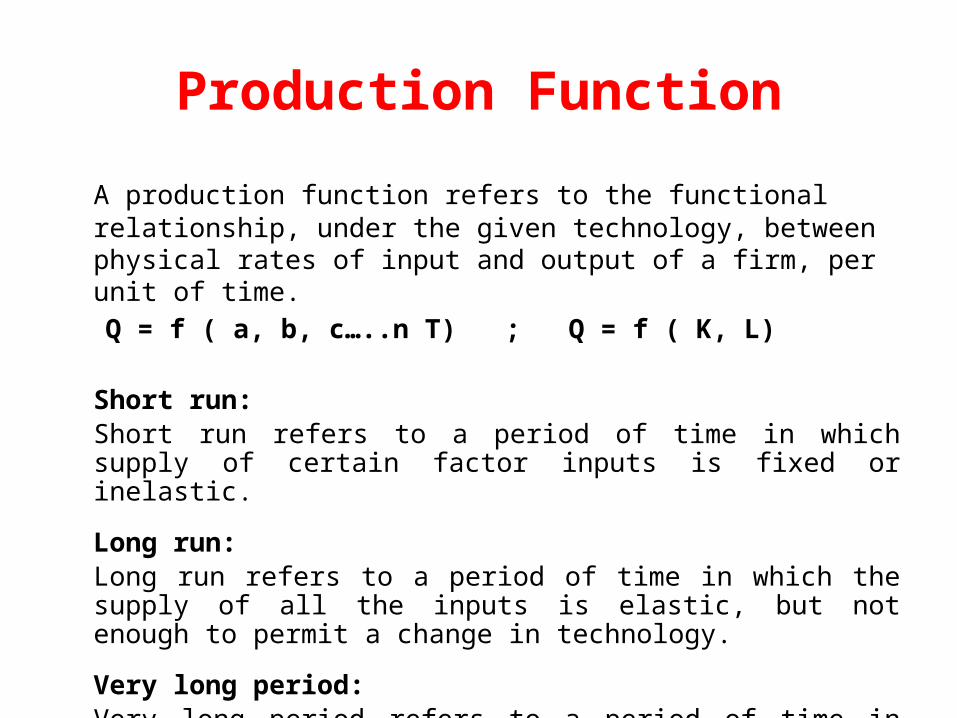
A production function refers to the functional relationship, under the given technology, between physical rates of input and output of a firm, per unit of time.Q = f ( a, b, c…..n T) ; Q = f ( K, L)

Short run: Short run refers to a period of time in which supply of certain factor inputs is fixed or inelastic.

Long run: Long run refers to a period of time in which the supply of all the inputs is elastic, but not enough to permit a change in technology.

Very long period: Very long period refers to a period of time in which along with all other factor inputs, the technology of production can also be changed.

Production Function

Key Terms in Production Analysis

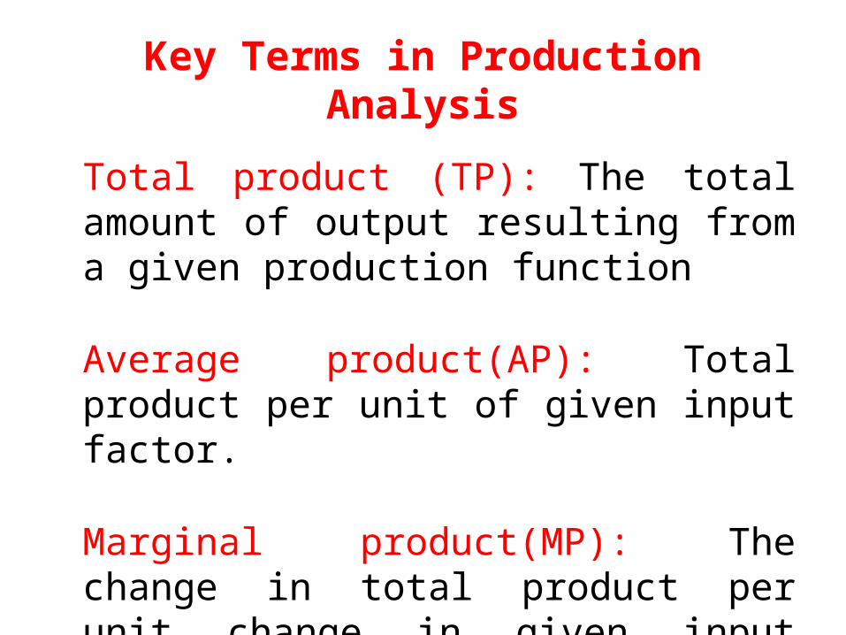
Total product (TP): The total amount of output resulting from a given production function

Average product(AP): Total product per unit of given input factor.

Marginal product(MP): The change in total product per unit change in given input factor.

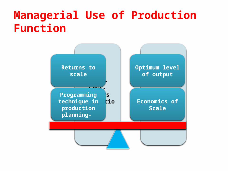
Managerial Use of Production Function

Least-Cost-Factors

combinationBreakeven Qty

Economics of Scale

Optimum level of output

Programming technique in production planning-

Returns to scale

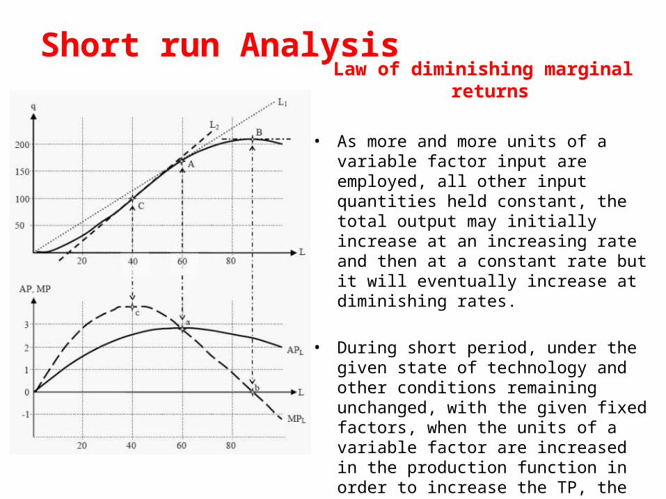
Short run AnalysisLaw of diminishing marginal returns

• As more and more units of a variable factor input are employed, all other input quantities held constant, the total output may initially increase at an increasing rate and then at a constant rate but it will eventually increase at diminishing rates.

• During short period, under the given state of technology and other conditions remaining unchanged, with the given fixed factors, when the units of a variable factor are increased in the production function in order to increase the TP, the TP initially may rise at an increasing rate and after a point it tends to increase at a decreasing rate because the MP of the variable factor in the beginning may tend to rise but eventually tend to diminish.

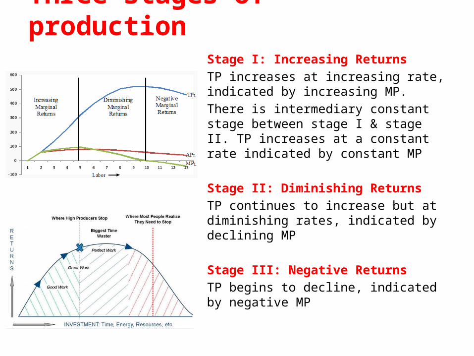
Three stages of productionStage I: Increasing Returns TP increases at increasing rate, indicated by increasing MP. There is intermediary constant stage between stage I & stage II. TP increases at a constant rate indicated by constant MP

Stage II: Diminishing ReturnsTP continues to increase but at diminishing rates, indicated by declining MP

Stage III: Negative Returns TP begins to decline, indicated by negative MP

Production function with Two Variables

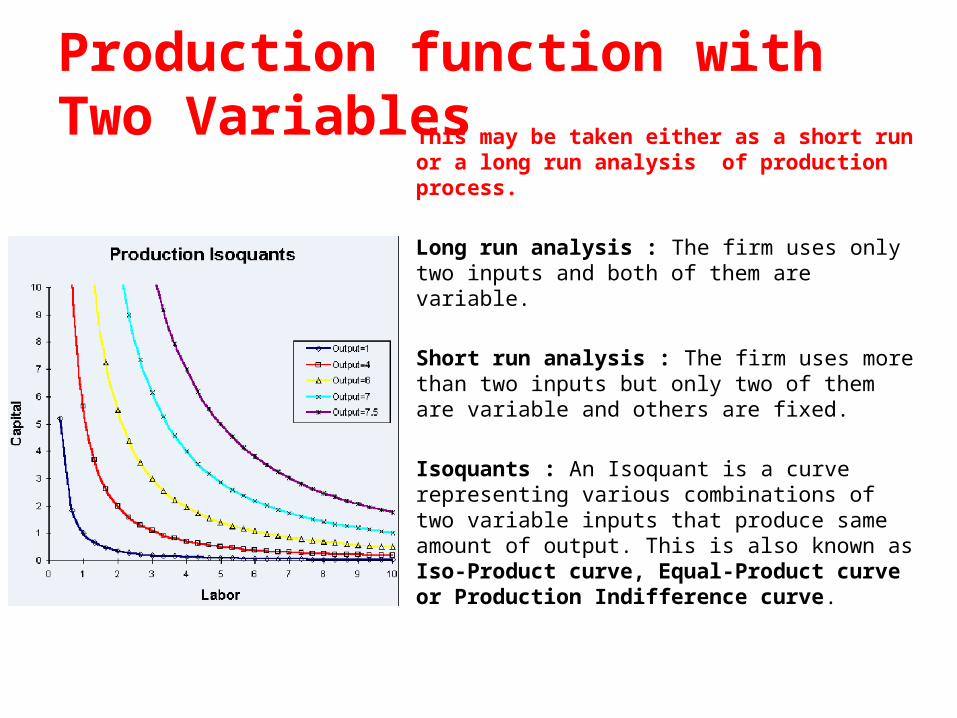
This may be taken either as a short run or a long run analysis of production process.

Long run analysis : The firm uses only two inputs and both of them are variable.

Short run analysis : The firm uses more than two inputs but only two of them are variable and others are fixed.

Isoquants : An Isoquant is a curve representing various combinations of two variable inputs that produce same amount of output. This is also known as Iso-Product curve, Equal-Product curve or Production Indifference curve.

Properties of Isoquants

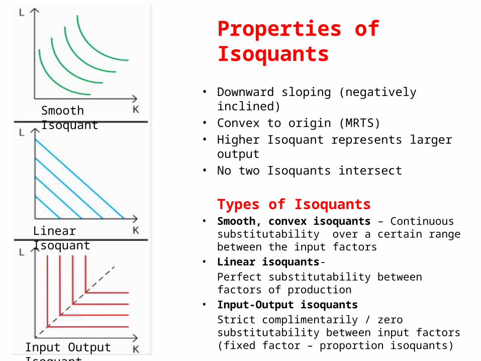
• Downward sloping (negatively inclined)• Convex to origin (MRTS)• Higher Isoquant represents larger output• No two Isoquants intersect

Types of Isoquants• Smooth, convex isoquants – Continuous

substitutability over a certain range between the input factors

• Linear isoquants-Perfect substitutability between factors of production

• Input-Output isoquantsStrict complimentarily / zero substitutability between input factors (fixed factor – proportion isoquants)

Linear Isoquant

Input Output Isoquant

Smooth Isoquant

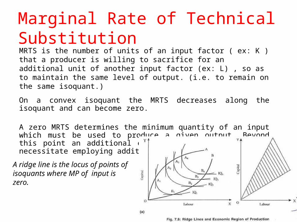
Marginal Rate of Technical SubstitutionMRTS is the number of units of an input factor ( ex: K ) that a producer is willing to sacrifice for an additional unit of another input factor (ex: L) , so as to maintain the same level of output. (i.e. to remain on the same isoquant.)

On a convex isoquant the MRTS decreases along the isoquant and can become zero.

A zero MRTS determines the minimum quantity of an input which must be used to produce a given output. Beyond this point an additional employment of one input will necessitate employing additional units of other input.

A ridge line is the locus of points of isoquants where MP of input is zero.

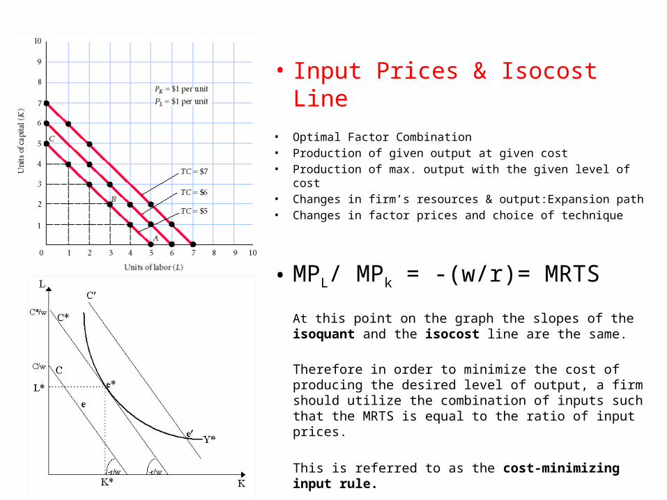
• Input Prices & Isocost Line

• Optimal Factor Combination• Production of given output at given cost • Production of max. output with the given level of cost• Changes in firm’s resources & output:Expansion path• Changes in factor prices and choice of technique

• MPL/ MPk = -(w/r)= MRTS

At this point on the graph the slopes of the isoquant and the isocost line are the same.

Therefore in order to minimize the cost of producing the desired level of output, a firm should utilize the combination of inputs such that the MRTS is equal to the ratio of input prices.

This is referred to as the cost-minimizing input rule.

Law of Return to Scale

The percentage increase in output when all inputs vary in the same proportion is known as returns to scale. It obviously relates to greater use of inputs maintaining the same technique of production.

Three Situations of Returns To Scale

Increasing Returns to Scale – Output increases by a greater proportion than the increase in input.

Constant Returns to Scale – Output increases in same proportion as increase in inputs.

Decreasing Returns to Scale – Output increases in a lesser proportion than the increase in input.

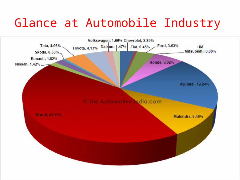
Glance at Automobile Industry

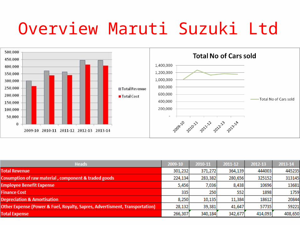
Overview Maruti Suzuki Ltd

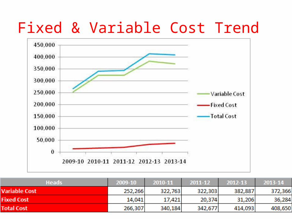
Fixed & Variable Cost Trend

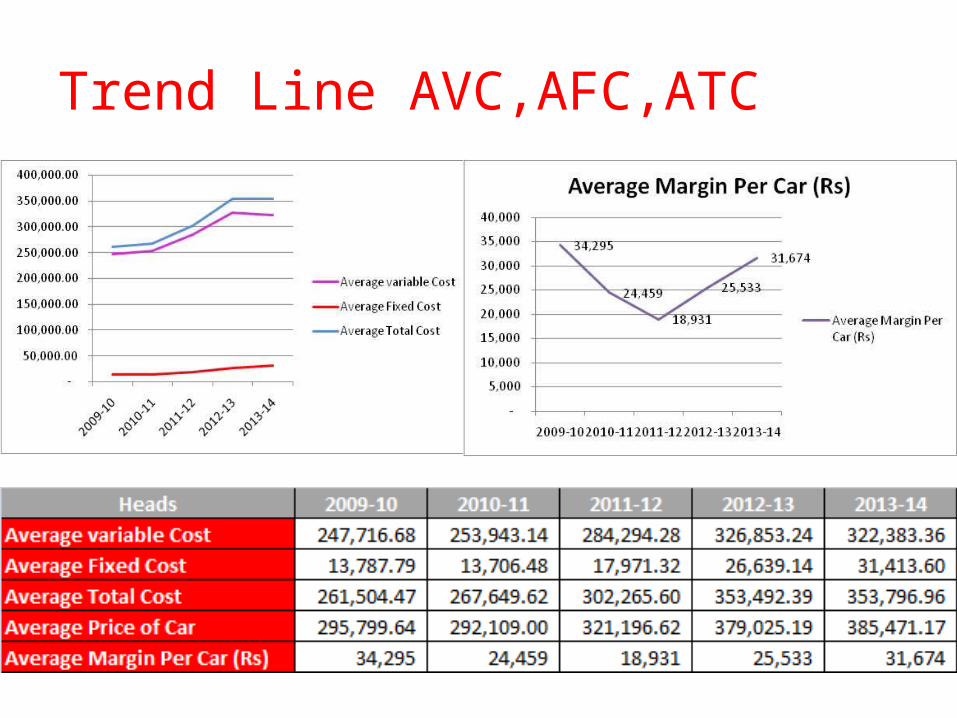
Trend Line AVC,AFC,ATC

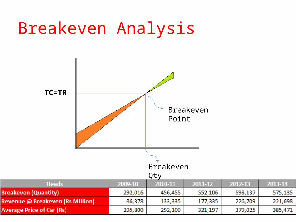
Breakeven Analysis

Breakeven Qty

Breakeven Point

TC=TR

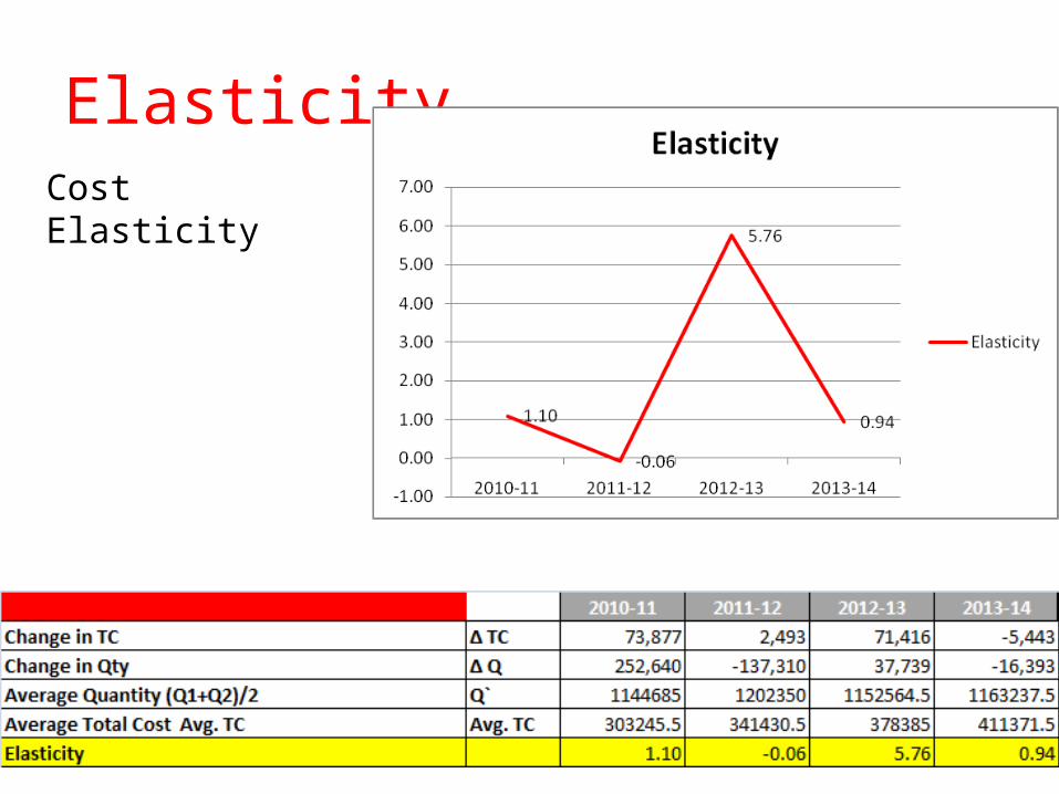
Elasticity

Cost Elasticity