Product and Price Competition in a Two-Dimensional...

Product and Price Competition in a Two-Dimensional Vertical Differentiation ModelAuthor(s): Mark B. Vandenbosch and Charles B. WeinbergSource: Marketing Science, Vol. 14, No. 2 (1995), pp. 224-249Published by: INFORMSStable URL: http://www.jstor.org/stable/184200Accessed: 05/09/2010 14:38

Your use of the JSTOR archive indicates your acceptance of JSTOR's Terms and Conditions of Use, available athttp://www.jstor.org/page/info/about/policies/terms.jsp. JSTOR's Terms and Conditions of Use provides, in part, that unlessyou have obtained prior permission, you may not download an entire issue of a journal or multiple copies of articles, and youmay use content in the JSTOR archive only for your personal, non-commercial use.

Please contact the publisher regarding any further use of this work. Publisher contact information may be obtained athttp://www.jstor.org/action/showPublisher?publisherCode=informs.

Each copy of any part of a JSTOR transmission must contain the same copyright notice that appears on the screen or printedpage of such transmission.

JSTOR is a not-for-profit service that helps scholars, researchers, and students discover, use, and build upon a wide range ofcontent in a trusted digital archive. We use information technology and tools to increase productivity and facilitate new formsof scholarship. For more information about JSTOR, please contact [email protected].

INFORMS is collaborating with JSTOR to digitize, preserve and extend access to Marketing Science.

http://www.jstor.org

http://www.jstor.org/action/showPublisher?publisherCode=informs

http://www.jstor.org/stable/184200?origin=JSTOR-pdf

http://www.jstor.org/page/info/about/policies/terms.jsp

http://www.jstor.org/action/showPublisher?publisherCode=informs

MARKETING SCIENCE Vol. 14, No. 2, 1995

Printed in U.S.A.

PRODUCT AND PRICE COMPETITION IN A TWO-DIMENSIONAL VERTICAL

DIFFERENTIATION MODEL

MARK B. VANDENBOSCH AND CHARLES B. WEINBERG The University of Western Ontario The University of British Columbia

In this paper, the one-dimensional vertical differentiation model (Shaked and Sutton 1982, Moorthy 1988) is extended to two dimensions and an analysis of product and price competition is presented. A two-stage game theoretic analysis in which two firms compete first on product positions and then on price is conducted. Closed form equilibrium solutions are obtained for each stage in which competitors are unrestricted in their choices of price or product positions. A significant finding of this research is that unlike the one-dimensional vertical differentiation model, firms do not tend towards maximum differentiation, although this solution is possible under certain conditions. When the range of positioning options on each of the dimensions is equal, MaxMin product differentiation occurs. That is, in equilibrium, the two firms tend to choose positions which will represent maximum differentiation on one dimension and minimum differentiation on the other dimension. (Competitive Strategy; Game Theory; Product Policy; Pricing Research)

1. Introduction

Many marketing managers are regularly faced with decisions about what product fea-

tures to offer and what price to charge. These decisions need to consider not only what

the customer wants, but also how competitors will act. Consider the following illustrative

example (see Rangan et al. 1992 and Moriarty 1985). In 1984, the management at Signode Industries, Inc. Packaging Division (Signode)

was finding it increasingly difficult to maintain or increase profitability levels in the steel

strapping industry (Moriarty 1985). 1 Over the years, the competitors in the industry had

stabilized their market position and relative price separation. Signode had the highest share and the highest average price in the market. It was able to maintain this position because it offered significantly more services than any of its competitors. Signode's com-

petitors were relatively undifferentiated from each other and tended to price their strapping at a consistent discount to Signode. While historically Signode was able to differentiate

its steel strapping from its competitors (e.g., by offering special grades), the quality of

the strapping offered to the market was now equal for all competitors. Given limited

' Steel strapping is used to bind products together for shipment. For example, steel strapping is used to bind quantities of lumber, stacks of bricks, and rolls of steel.

224

0732-2399/95/1402/0224$0 1.25 Copyright C 1995, Institute for Operations Research and the Management Sciences

PRODUCT AND PRICE COMPETITION 225

potential for innovation in the steel strapping industry, the market appeared to have moved to an equilibrium state with Signode positioned as the high (but now standard) quality, high service firm with a premium price.

The situation in the steel strapping industry is not unique.2 Competitors in most markets must decide on price as well as the positioning of their offerings on more than one dimension (i.e., quality, services offered, etc.). Recently, competitive multidimensional positioning has received considerable attention (e.g., Hauser 1988; Kumar and Suharshan 1988; Gruca et al. 1992; Carpenter 1989). In this paper, the one-dimensional vertical differentiation model (Shaked and Sutton 1982, Moorthy 1988) is extended to two dimensions and an analysis of product and price competition is undertaken. A two-stage game theoretic analysis in which two firms compete first on product positions and then on price is conducted. Closed form equilibrium solutions are obtained for each stage in which competitors are unrestricted in their choices of price or product positions.

A significant finding of this research is that unlike the one-dimensional vertical differentiation model, firms do not tend towards maximum differentiation, although this solution is possible under certain conditions. When the range of positioning options on each of the dimensions are equal, MaxMin product differentiation occurs. That is, in equilibrium, the two firms tend to choose positions which will represent maximum differentiation on one dimension and minimum differentiation on the other dimension. This result mirrors the situation in the steel strapping industry.

This paper is structured as follows. Section 2 reviews the relevant literature in both economics and marketing. Section 3 introduces the model by outlining its assumptions and comparing it to existing models. Section 4 develops the price equilibrium while ?5 develops the product equilibrium. This is followed in ?6 by a discussion of conclusions and implications. Section 6 also discusses the effects of relaxing some model assumptions. Finally, ?7 provides directions for future research.

2. Literature Review

Product differentiation research has attracted considerable attention in both economics and marketing (Lancaster 1990, Ratchford 1990). Using Lancaster's notion of product space (Lancaster 1971, 1979), two variants of product differentiation can be distinguished: horizontal (variety) differentiation and vertical (quality) differentiation. In a horizontally differentiated product space, tastes vary across the population resulting in a distribution of individual ideal characteristic levels. In a vertically differentiated product space, all consumers agree that more of a characteristic is always better, but they vary in their willingness to pay for this characteristic. Marketers have traditionally modeled vertical and horizontal characteristics using the vector model and the ideal point model respectively (Shocker and Srinivasan 1979). Ratchford (1979) shows how the development of these empirically based models is linked to Lancaster's goods-characteristics theory.

Much of the differentiation research is related to the horizontal differentiation model developed by Hotelling (1929) who advances the Principle of Minimum Differentiation. That is, at equal prices, competing firms whose products are differentiated on a single horizontal dimension will choose the same product location at the center of the market. d'Aspremont et al. (1979) found that when price competition was considered, minimum differentiation in a Hotelling environment leads to severe price cutting and a price equilibrium only at p * = p = 0 (assuming marginal cost = 0).3 Using a different consumer

2 As Rangan et al. ( 1992) note, not all markets face the same level of market maturity, agreement on critical product/offering features or competitive focus, but many do. Other published case studies of firms facing similar market situations include "Sealed Air Corporation" (Dolan 1982) and "Federated Industries" (Dolan 1984).

3 Economides ( 1986) extends Hotelling's model to two dimensions. He shows that a price equilibrium exists for all symmetrical locations whereas such an equilibrium does not in the linear model.

226 MARK B. VANDENBOSCH AND CHARLES B. WEINBERG

cost minimization function, d'Aspremont et al. obtain a unique locational equilibrium which implies maximum product differentiation.

From the analyses of Hotelling and d'Aspremont et al., it is apparent that two forces determine the locational equilibrium: a demand force (a desire to increase the share of consumers to which the firm is the closest) which draws the firms together and a strategic force (a desire to reduce price competition) which causes the firms to differentiate. These forces can be applied to the vertical differentiation case as well.

Gabszewicz and Thisse (1979) and Shaked and Sutton (1982), building on research by Mussa and Rosen (1978), develop duopoly models using the vertical differentiation assumption. These researchers show that the desire to reduce price competition (the strategic effect mentioned above) results in a product equilibrium where firms are located at the extreme ends of the quality spectrum. Moorthy (1988) extends the basic model by incorporating variable production costs and allowing consumers the opportunity not to buy. His equilibrium analysis shows that firms choose products which are differentiated (though not maximally).

The models proposed by Hauser (1988) and Lane (1980) represent variations of the horizontal differentiation model. Hauser analyzes pricing and positioning strategies using the DEFENDER consumer model (Hauser and Shugan 1983) in which products are differentiated in a two-dimensional per dollar perceptual map. Although the per dollar perceptual map permits only "more is better" attributes similar to a vertical differentiation model, the limited product positioning options makes the resulting positioning equilibrium behave in much the same way as the horizontal differentiation model. Hauser imposes the restriction that feasible products must lie on the circumference of a quarter circle inscribed in the positive quadrant. In effect, this reduces the positioning decision to one dimension (Hauser 1988, p. 79). Like Hotelling's model, each consumer has an ideal product in this dimension at constant prices. The product equilibrium consists of minimum differentiation at equal prices and maximal differentiation when both prices and product positions are considered. Lane's model represents brands in two-dimensional space on the basis of product characteristics where price is considered separately. Lane's assumption of a single technology curve restricts the product choice to a one-dimensional decision in much the same way as Hauser's "quarter circle" assumption.

Several researchers have extended the one-dimensional product differentiation models to multiple dimensions (dePalma et al. 1985; Neven and Thisse 1990; Economides 1989).4

dePalma et al. (1985) show that the Principle of Minimum Differentiation is restored when "products and consumers are sufficiently heterogeneous". They develop a model which implies that when inherent differences within firms and consumers become large, products are differentiated even though they have the same physical location. Therefore, the strategic effect (the desire to reduce price competition) is limited and the demand effect dominates. The authors state that the inclusion of heterogeneity in both firms and consumers "amounts to adding a second, nonspatial dimension" (p. 779).

Economides (1989) and Neven and Thisse (1990) both analyze a two-dimensional vertical and horizontal differentiation model in which firms compete on quality, variety, and price. Economides assumes that the horizontal (variety) choice takes place before the vertical (quality) choice. In addition, he assumes that marginal costs are increasing in the quality. This modeling framework leads to maximum variety differentiation and minimum quality differentiation. In the Neven and Thisse model, firms first choose their product, consisting of two characteristics, and subsequently choose their price. Assuming zero marginal costs, these researchers find a product equilibrium that exhibits maximum

4 A number of other two-dimensional models have been developed (i.e., Carpenter 1989; Kumar and Sud-

harshan 1988; Choi et al. 1990; Horsky and Nelson 1992). These models focus on different issues than our

model.


differentiation on one dimension and minimum differentiation on the other. However, the maximally differentiated dimension can either be the quality-or variety dimension.

The model described in this paper employs analysis procedures similar to those used by Neven and Thisse. A key difference in our model is the fact that both dimensions are vertical (quality) dimensions. This takes into account situations in which consumers evaluate offerings with more than one type of quality (like product quality and service quality in the Signode example). Our model also assumes that consumers are using a consistent decision rule to evaluate each of the dimensions. We find that this structure can lead to product equilibria which are different from those described in Neven and Thisse.

3. Model Assumptions

The two-dimensional vertical differentiation model analyzed in this paper is based on the following assumptions:

(1) There are two firms, indexed 1 and 2, who each choose one product to market. Products are comprised of nonnegative valuations on two characteristics, x and y. The characteristics are analogous to perceptual dimensions or product attributes and are assumed to be orthogonal. Thus, each firm's product is defined as a point (xi, yi), where

x, E [Xmin, Xmax] and yi E [Ymin, ymax]

(2) Consumers are assumed to prefer more of each characteristic to less. For example, personal computers may be described on two dimensions like "power" and "ease of use" in which consumers always prefer "more powerful" and "easier to use" computers holding all other attributes constant. It is assumed that price enters negatively into the consumer's valuation equation.

(3) Consumers are able to observe product characteristics and prices before they make their purchase decision. Consumers' reservation prices (R) for a product in this market may vary but are high enough to ensure that all consumers buy. In addition each consumer is restricted to purchasing one unit-either from firm 1 or firm 2. A typical consumer's valuation equation can be described by a standard individual level vector model in which utility is expressed in dollar units (Srinivasan 1982) (the consumer subscript is omitted):

U = R + 01xi + 02Yi-Pi for i = 1, 2 (1)

where pi is the price of firm i's product.

The consumer will choose the product from the firm which maximizes (1). Consumer heterogeneity is captured by the two parameters, 01, 02.

(4) The parameters, 01, 02, are assumed to be uniformly distributed over the population. Since one characteristic may, on average, be more important than the other, the range of the parameter distribution may be different for each characteristic. Without loss of generality, both of these ranges can be restricted to [0, 1]. This can be accomplished by choosing the appropriate scale for each of the characteristics (x, y).

(5) Products are assumed to have a constant marginal cost set, without loss of generality, to zero regardless of product position. Though this assumption is obviously un- realistic, the analysis is significantly simplified while retaining the strategic effects of product positioning. In addition, it is assumed that there are no fixed costs. This eliminates the need to study entry and exit decisions. The effects of a departure from the constant marginal cost assumption are discussed in ?6.

The two-dimensional vertical differentiation model is designed to provide a direct extension of the one-dimensional vertical differentiation model. It is most similar to the model presented by Shaked and Sutton (1982) because marginal costs are assumed to be constant (and equal to zero) for all product positions. Since the major emphasis of


this research is to assess the nature of competitive behavior, this reduction in complexity seems reasonable. An obvious extension of the model would be to incorporate position- dependent variable costs in a manner similar to Moorthy ( 1988).

The model presented here is also quite similar to Hauser ( 1988). Both models use two dimensions to characterize the product space and assume that consumers have ho- mogeneous perceptions of the products. Hauser assumes that perceptions can be ratio scaled and thus, similar to the above model, higher levels on a perceptual attribute are always better. However, there are a number of important differences. In Hauser's model of utility, the value of the products' perceptual characteristics is divided by price whereas price enters in a linear fashion in our model. This difference represents different methods of comparing prices between products. Hauser's model assumes consumers compare relative prices where our model assumes consumers compare absolute price differences. Empirical research by Hauser and Urban ( 1986) has shown that these two criteria have performed equally well in assessing price response to durables.

Defining the Indifference Surface

In the analysis of the vertical differentiation model, there are two generic types of product positioning competition: asymmetric characteristics and dominated characteristics. Asymmetric characteristics competition is defined as competition between firms when each firm has a relative advantage on one of the two characteristics (see Figure 1 ). For example, if the two characteristics which describe the personal computer market are "ease of use" and "power", Apple computers would have a relative advantage over IBM on the "ease of use" dimension while IBM would have the relative advantage over Apple on the "power" dimension.' Dominated characteristics competition is defined as competition between firms when one firm has a relative advantage on both characteristics. This situation is typical of competition between different "models" of a similar technology. Competition between XT, AT, 386 and 486 personal computers would be an example of dominated characteristics competition.

For both types of competition, the relative positions of the products can be described by taking a ratio of the absolute differences in the characteristic levels of the two products. The ratio (x1 - x2)/(y2- Yi) is equal to the tangent of the angle between the horizontal axis and a line from the origin perpendicular to a line joining the two products. This angle of competition illustrates the relative positioning advantage of the firms and becomes important in the determination of the demands for each product. It should be noted that each angle represents the set of alternative product positionings that maintain the same relative separation.

Figure la provides an example of asymmetric characteristics competition. Without loss of generality, it is assumed that firm 1's product has the advantage on x and firm 2's product has the advantage on y. Consumers in this market decide to purchase the product which maximizes their utility as defined by (1). This comparison leads to a set of consumers who are indifferent to choosing either product. This set is a line which intersects the set of consumer types. Consumers types above the indifference line choose product 2 and consumers below the line choose product 1. In 01 X 02 space, this indifference line is defined as:

- (P2-P1) + (x1- X2) (2) (Y2-Y1) (Y2-Y1)

Figure l b illustrates this indifference line at equal prices. The slope of this indifference line is the negative inverse of the slope of the line connecting the two products in x X y

I Notice here that these quality dimensions are designed into the machines and may not be reflected directly in variable costs. This is especially true for the "ease of use" dimension.


a) Characteristics Space b) Parameter Space (P1= P2)

y 02

2 Demand 2

1 | / Demand 1

x 1 01

FIGURE 1. Relationship Between Characteristics Space and Parameter Space in the Two-dimensional Vertical Model with Asymmetric Characteristics.

space. Thus, the market share of each of the products is dependent on the angle of competition defined by the relative product positions (a in Figures 1 a and Ib). In addition, the terms (x, - x2) and (Y2- Yl) provide a measure of absolute product differentiation. The difference between prices, P2 - Pl, shifts the indifference line up or down. Firms deviate from equal prices to the extent that their respective profitability is increased. In 01 X 02 space, the demand for each product is defined by the area above (product 2) or below (product 1) the indifference line.

The relationship between x X y space and 01 X 02 space (via the angle of competition) clearly illustrates the advantage of a superior product position. Intuitively, the desirability of a firm's product is dependent on the relative characteristics of the two products. If one product has more of x but both products have virtually the same amount of y, it would be expected that, at equal prices, this product would capture most of the market. Con- versely, if each product had approximately equal absolute product differentiation advan- tages on their respective dominant characteristics, at equal prices, they would each obtain approximately 50% of the market.

Dominated characteristics competition differs slightly from asymmetric characteristics competition due to the presence of a superior and an inferior product (Figure 2a). Without loss of generality, it is assumed that firm 2's product is the superior product. Analysis proceeds in the same manner as with asymmetric characteristics competition. As Equation (2) holds, the slope of the indifference line is the negative of the slope of the line connecting the two products in x X y space. The slope of the indifference line is negative, with the angle of competition being greater than 900 (Figure 2b). As would be expected, at equal prices product 2 captures the entire market. There must exist a lower price for the inferior product before any consumer will purchase it. This is similar to results obtained using the one-dimensional vertical differentiation model (Moorthy 1988).

4. Price Equilibrium

There are a number of approaches open to the analysis of product design and price competition in the environment described in the previous section (see Moorthy 1985, Tirole 1988 for reviews). This paper will analyze a sequential game in which firms first choose their product characteristics and subsequently choose their price. In this approach, the subgame-perfectness criterion is used. A subgame perfect equilibrium consists of a product choice for each of firms 1 and 2 such that neither firm would choose a different


a) Characteristics Space b) Parameter Space (P2> PI)

y 02 Y (32~~~

Demand 2

Demand 1

x 1 01

FIGURE 2. Relationship Between Characteristics Space and Parameter Space in the Two-dimensional Vertical Model with Dominated Characteristics.

product unilaterally, recognizing that the profitability of all product selections will be determined on the basis of the price equilibrium that follows (Moorthy 1985). The analysis procedure proceeds by backwards induction. The price equilibrium will be analyzed first followed by the product choice equilibrium.6 Based on the research of Caplin and Nalebuff ( 1991, p. 29), the assumptions of our model ensure the existence and uniqueness of a price equilibrium.

Since costs are assumed to be constant (and zero) regardless of position, the profit function for firm i (i = 1, 2) is defined as l1i (pi, pj) = piDi(pi, pj) for i # j. A noncooperative (or Nash) price equilibrium is a pair of prices (p*, pJ ) such that:

li(pi ,P7)?ll (pi,P*), Vpi?0, i,j=1,2, and i=#j.

The price equilibrium under asymmetric characteristics competition will be analyzed before dominated characteristics competition. The price equilibria for the asymmetric characteristics case will be denoted by single or multiple asterisks (*) while the price equilibria for the dominated characteristics case will be denoted by single or multiple daggers (t).

Asymmetric Characteristics Competition

Under asymmetric characteristics competition, the indifference line in 01 X 02 space is defined by (2). This line is positively sloped with angle

a = tan-l( XI X2 ).7 Y2 -YI

When product positions are fixed, the indifference line is shifted up or down with changes in (P2 - Pi). These shifts alter the demand (and profits) for each firm. The demand effects of price changes will be analyzed from the perspective of firm 1. Thus, P2 will be taken as given (denoted ff2). Analysis undertaken from the perspective of firm 2 would yield parallel results.

6 The following analysis describes the price equilibria. In some instances, second-order conditions are calculated to show that they are satisfied. In all other instances, second-order conditions have been analyzed by inspection.

7 Note that in the numerator, firm 2's characteristic level is subtracted from firm l's level whereas in the denominator firm l's characteristic level is subtracted from firm 2's level. Under asymmetric characteristics competition, both (xl - x2) and (Y2 - y') are positive.


(2

(0,1)

Indifference Indifference ( Line atp1 Lineaatp

Indifference Line at p n / Indifference

Line at p |

(0,0) /a

(1,0) 01

Note: Demand for firm 1 is the area below the Indifference Line. FIGURE 3. Location of the Indifference Line at Boundary Levels of p, (given P2).

Given P2, four boundary price levels for firm 1 can be defined (see Figure 3). p' is defined as the lowest price at which no consumers are willing to purchase from firm 1. At this price, the indifference line passes through (1, 0). pj is defined as the highest price at which all consumers purchase from firm 1. This occurs when the indifference line passes through (0, 1). p' and pi can be considered to be the upper and lower bounds on the prices that firm 1 will charge for its product given 1f2. Demand is not affected by price levels outside of this range. The two remaining key price levels, p7 and p7, occur when the indifference line passes through (0, 0) and ( 1, 1 ) respectively. At each of these two prices, one of the most extreme consumer types is indifferent between the two products. These prices also define levels at which the shape of the demand functions change.

The functional form of the four boundary prices can be found by replacing 01 and 02 in (2) with the boundary point coordinates. This results in the following price equations:

P1=12+(X1X2), (3)

1pm=f2 + (xI -X2) (Y2 YI), P' = ~~~~~~~~~~~~(4)

P=1 P2, (5)

P'= P2-(Y2 YI). (6)


All of these prices are increasing in 1^2. When the terms appear, the price equations are also increasing in (xl - x2) and decreasing in (Y2 - yl). Indirectly, this implies that the prices are increasing in a. That is, the greater firm 1's relative positioning advantage over firm 2, the higher the price firm 1 is able to charge to generate a similar demand level.8

As firm 1 decreases its price from p', two distinct cases arise depending on the size of a. Characteristic x dominance occurs when a ? 450 [(xl - x2) 2 (y Y )]. This means that the absolute product differentiation on characteristic x is greater than or equal to the absolute product differentiation on characteristic y. When characteristic x dominance holds, Pi < pi < pm < p'. That is, the indifference line passes through (1, 1) in the space defining consumer types before it passes through (0, 0) when prices are decreased from p 1'.

When a < 45?, characteristic y dominance holds and pi < pm < p' < p'. This alternative ordering of key prices has an impact on the price equilibrium calculations. Therefore, the characteristic x dominance and characteristic y dominance cases are analyzed separately. Note that the case when neither characteristic dominates, a = 45?, can be represented by either type of dominance. When a = 00 or 900, the product choice reduces to one dimension.

Characteristic x dominance. In 01 X 02 space, as firm 1 decreases its price from p ', the indifference line shifts upward. Three distinct demand regions can be defined on the basis of the geometric structure of the model. These regions correspond to the rate of change in demand for a unit shift in price (see Figure 3). In region R 1, demand for firm 1 increases (as a function of prices) at an increasing rate. This region is defined by the price range pm < p, c p'. In R , where p'1 < p ? pm, demand for firm 1 increases at a constant rate. Finally, in R3, where pl < p, c p', the demand for firm 1 increases at a decreasing rate.9

In R 1, the possible prices that can be charged by firm 1 can be viewed as a continuum from p ' to pm. Let z1 represent the proportion of the distance pi is from the p end of the continuum. At pi = p', z1 = 0 and at pi = pm, z1 = 1. In the space defining the consumer types, z, represents the distance from the horizontal axis to the point where the indifference line meets the right side of the "square" of consumer types (see Figure 4). Mathematically z, is defined as follows:

p _ P Pi _ j32-p1 +(XI -X2)

pI - uPi (Y2 YI )

The demand for firm 1 in R l, D 1, is the area of the triangle formed by the indifference line and the edges of consumer types. In this triangle, the angle a is known as well as the height of the triangle (zl). The formula for the area of a triangle, A = 1 (base)(height), is used to calculate D1. Since cot a = (base)/ (height), D can be defined as

DI=-(z )2cot a, 2

1P2 -PI + (X1 2) \ DI = ( ) ) cot a. (8)

8 It is interesting to note that the density function of consumer types does not influence these price relationships. Firm 2's rate of change in demand in these regions is the complement to firm 1 since

Demand2 + Demand, = 1.


02

1

,s' / - Indifference Line

00~ ~ z

1 1

#0 ~ 0

? I P00PI

Demand 2.Dtriaino Demand in

1 11p2p~1\ 0 From (8), it can be seen that demand depends on both prices and product positions. Proceeding similarly, demand in R2 and R3 is as follows:

DI =cot1 -Icot +ot)cat, (10) 2 (X (x-x2)-(Y2 -Y ))

D3 = I1-1 Icot a + 1(P2 -A

) cot a. ( 10)

Combining Equations (8), (9) and (10), the demand for firm 1 as a function of Pi can be determined (Figure 5). Since it is assumed that all consumers buy, the demand for firm 2 is simply 1 - D1. Each demand curve is comprised of a convex, linear and concave segment (corresponding to the regions defined above). Therefore, one of three possible price equilibria may result under characteristic x dominance. These equilibria will be denoted by the price regions in which the equilibria lie:'0 strictly convex segment of firm 1 's demand curve-strictly concave segment of firm 2's demand curve (R k); linear segments of firm l's and firm 2's demand curves (R2 ); and strictly concave segment of firm l's demand curve-strictly convex segment of firm 2's demand curve (R3 ).

Analysis of the price equilibria. Analysis ofthe price equilibria proceeds by considering each of the regions beginning with R2. The mathematical proofs are available on request from the authors. In R2, the demand equations for the two firms are linear in prices

10 An analysis from the perspective of firm 2 shows that the same regions apply for both firms.


Market Share Demand 1 Demand 2

141...

I p~~n pm pu Price1

FIGURE 5. Demand as a Function of pi (given p2) Under Characteristic x Dominance.

and the profit functions are quadratic in prices. The first-order conditions of the profit functions have a single solution given by:

* (11)

Pi ~~ 6

* 2(x -x2)+Q2-yi)1

Since the first-order conditions are necessary, these prices are the price equilibrium prices provided they belong to the intervals defining R 2. These intervals are:

EE e[pn(p'), p7(p*')] an E [pn(p*), pm(p*)].

These restrictions yield two conditions which must be satisfied for Equations (11 I) and (2) to represent the price equilibrium in Ri2. First, p*' pn(p*) (as given by (5)) is

satisfied when:

(XI /. X2X .. (Y2 - YI),(A)

Second, p1' pm(p1') (as given by (6)) is satisfied when:

(X X2)?(Y2-YI). (B)

Notice that (A) and (B) are equal and always true under characteristic x dominance. Therefore, there is no need to calculate the equilibrium prices in Rf- or Rn 3 By reformulating the pricing equations, it can be shown that py: E [pn(p p'(p*)] only when both conditions (A) and (B) are satisfied.


Characteristic y dominance. Under characteristic y dominance, the angle of competition (a) is <45? [(xl - x2) < (y2- Yl)]. Price equations (3)-(6) hold but now pi < p < p7 < p'. Using the same procedure as outlined under characteristic x dominance, demand in each of the regions can be defined as a function of prices and a.

In R2, the demand equations are linear in prices. The first-order conditions of the profit functions have a single solution given by:

** 2(Y2-Y1)+(xl-x2) (13) 6

= 4 (y2-Y1y)--(xl-x2) P2 = - 6 (14)

Since the first-order conditions are necessary, these prices are the price equilibrium prices provided they belong to the intervals defining R 2. These intervals are:

E=*e[pm(p* *) pn(p~*I and m(* ,pnp Pi E[1 (2 ), P(2 )] and P 2 E[2 (1 ), P(1)]

These restrictions yield two conditions:

(xil- x2) ' (Y2 - YI), (C)

(xl-x2)?(y2-Y1)- (D)

Notice that conditions (C) and (D) are equal and always true under characteristic y dominance. In addition, (C) and (D) are the "reverse" of (B) and (A) respectively. By reformulating the pricing equations, it can be shown that p2 * E [pn(P *), P2(P1 *)] only when both conditions (C) and (D) are satisfied.

Dominated Characteristics Competition

This section discusses the price equilibrium solutions for the dominated characteristics case. The procedures employed are similar to those used in the asymmetric characteristics case. The reader interested in the product equilibrium results may wish to read ?5 before considering the price equilibrium results for the dominated characteristics case.

Characteristic x dominance. The indifference line (defined in (2)) applies as do the boundary price levels defined in (3 )-(6). Without loss of generality, it is assumed that firm 2's product is dominant. That is, x2 ? xi and Y2 ' y'. This implies that (xi - x2) < 0 and the slope of the indifference line is negative. Under characteristic x dominance, 900 < a < 1350. This implies that -(x1 - x2) > (Yj - yi). Under these conditions, the ordering of the price equations is p < p' < p'I < p .

Once again, analysis begins with region 2. In dRy, the price equilibrium is defined by:

t -2(x1-x2)-(y2-Y1) (1 ) Pi 6 (5

t -4(x,-x2) + (y2-y1) P2 6 (16)

This price equilibrium holds when the prices are within the range defining dR . That 1S,

P1 E [pl (pt), pn(pt)] and P(E [pl (pt), pn(pt)]. These restrictions yield two conditions. First, pt > pI (p2) is satisfied when:

-2(x - x2) (Y2 -Y i). (E)


Second, pI < P'1(P2) is satisfied when:

-(xi- x2) ? 2(y2- yl). (F)

By reformulating the pricing equations, it can be shown that p2 E [p2(P1), P12(P )] only when both conditions (E) and (F) are satisfied.

In region dR', the demand equations for the two firms are quadratic in prices. This results in profit functions for the two firms which are cubic in prices. Solving for pi and P2 yields the following price equilibrium: l

tt= V-8(xl-x2)(y2-Y1) (17) 8

tt 3V-8(xl - x2)(y2- y1) (18) P2 ~~~8

The price equilibrium in region dRA defined by (17) and (18) holds when ptt > pil (p2t) and pt p2 (ptt)* These inequalities are satisfied when condition (F) is violated or holds with equality. Condition (E) will continue to hold as will characteristic

I' ft t x dominance. Notice that when condition (F) holds with equality, pi = pi and p2

pt This indicates that equilibrium prices move continuously when parameters change such that the equilibrium moves from region dRx to dR 'X.

In region dR 3, the first-order conditions of the profit functions are quadratic in prices. The price equilibrium is not easily derived in this region as neither of the first-order conditions factor into simple functional forms. The exact solution has not been calculated as it is not required for the determination of the product equilibrium solutions.'2 This is due to the arbitrary choice of firm numbers. Region dRA from the perspective of firm 2 is identical to region dR3 from the perspective of firm 1.

Characteristic y dominance. Characteristic y dominance in the dominated characteristics case follows the same pattern established in previous sections. In this case, a 2 135' and p<l pi < p < pn

In dRy, the price equilibrium is defined by:

ttt = 2(Y2- y,) + (xl - x2) (19) Pi 6

ptt = 4(Y2- Yi) - (x1 - x2) (20) 6

This equilibrium is valid provided the following conditions hold:

-2(x - x2) ' (Y2- y ), (G)

-(X1- x2) < 2(y2- Yi). (H)

" The first-order condition for firm 1's profit function is a quadratic in pi. This equation can be factored into two roots: pi = P2 and P, = P2/3. The first root is equal to Equation (3): the price at which demand for firm 1 equals zero. Therefore, the second root is used in the equilibrium calculation. Substituting p, = P2/3

into the first-order condition of firm 2 yields:

3p2 - 4P2P1 + p2 + 2(x, - x2)(y2-y) = 0.

This equation is quadratic in P2. The larger of the two roots maximizes 112 (& r2/PO2 < 0 only for the larger root).

12 Ansari and Steckel ( 1992), using Mathematica, illustrate that the exact form of this equilibrium can be

found.


These conditions are simply the "reverse" of conditions (E) and (F). In dR 1, the demand equations for each firm are identical to those derived in dRX.

Therefore the price equilibrium defined by Equations ( 17 ) and ( 18 ) apply in this region as well. This price equilibrium is valid provided condition (H) is violated or holds with equality. Condition (G) will continue to hold as will characteristic y dominance. In addition, when (H) holds with equality, pit = pit and p = p. In both dR2 and dR I, because firm 1 controls the dominated product, the -equilibrium price for firm 1 is less than the equilibrium price for firm 2.

The price equilibrium in dR3 (like dR3 ) has not been calculated as it is not required for the determination of the product equilibrium solutions.

Summary

In summary, and anticipating the results of the next section, we have shown the existence of and determined the price equilibrium for any feasible product positioning equilibrium. Using a geometric representation, we see that the price equilibrium varies according to the region in which the competing products are positioned. Since the price equilibria are functionally related to the product positions, they can be incorporated directly into the product equilibrium analysis.

5. Product Equilibrium

The first stage of the sequential game involves the firms' simultaneous choice of product location. These product positioning decisions are dependent on the equilibrium prices which have been established above. Given the range of possible price equilibria (considering both characteristic dominance and demand region), several factors must be analyzed in order to choose the optimal product location.

The procedure used to determine the product equilibrium is as follows. First, an analysis is undertaken to determine which demand regions need to be considered for the product equilibrium analysis. The relative separation in positions between the two firms ((xl - x2) and (Y2 - yi)) determines the demand region and thus, the price equilibria which need to be considered. Second, the firms' profit functions in each of the relevant regions are calculated. Third, the first-order conditions of the profit functions, combined with the demand region restrictions, are used to determine the maximum profit equilibrium locations within each of the demand regions. Finally, the maximum profit levels in each of the relevant regions are compared to determine the highest profit equilibrium location representing the firm's optimal product choice (given the competitor's product choice).

Asymmetric Characteristics

In the asymmetric characteristics case, conditions (A)-(D) define the boundaries of the various price equilibria. By altering the values of xi, x2, y1 and Y2, it is possible to determine the relevant demand regions (and thus, price equilibria) for use in the product positioning subgame.

Consider the situation where xi and x2 are given (xi > x2) and y2, y1 are varied. (1) When Y2 = y', characteristic x dominance holds and conditions (A) and (B) are

satisfied. Therefore, the price equilibrium is in R2. (2) As (y2 - y1) is increased (by either raising y2 or lowering y1), (y2 - y1) will

eventually become larger than (xi - x2) so characteristic y dominance will hold. (A) and (B) are violated and (C) and (D) hold. Thus, the price equilibrium is in R 2

Now consider the situation where y1, and y2 are given (Y2 > y1) and xl, x2 are varied. ( 1 ) When xi = x2, characteristic y dominance holds and conditions (C) and (D) are

satisfied. The price equilibrium is in R2.


(2) When (xl - x2) is increased, (xi - x2) will become larger than (y2 - Yi) so characteristic x dominance will hold. (A) and (B) become satisfied and the price equilibrium will be in Rx.

Several points are worth noting. First, the sequences described above can be terminated at any step depending on the range of possible product positions. For example, the allowable increase in Y2 (given yi, xi and x2) may be restricted by the maximum level of y, (yrax). Second, since (A) = (B) (and (C) = (D)), the relevant demand regions for the price equilibrium move directly from R2 to R2 . The optimal positioning equilibrium will not occur in R 1, R 1, R 3, or R 3 . Finally, since both the demand functions and the equilibrium prices are continuous across regions, it follows that the profit functions are continuous as well.

The above analysis indicates that the profit functions in R 2 and R 2 must be considered in the derivation of the product equilibrium. In RL, the demand for firm 1 is given by ( 10) and the equilibrium price is given by ( 1 1 ). Multiplied together, these equations yield:

= (4(x- X2) (Y2-yl))2 (21) 36(x - x2)

For firm 2, the demand is given by D2 = 1 - D2 and the equilibrium price is given by ( 12). This yields a profit of

*= (2(xi - x2) + (Y2- y))2 (22) 2 ~~36(x1 - x2)

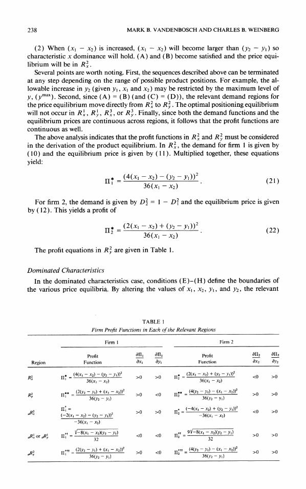
The profit equations in R2 are given in Table 1.

Dominated Characteristics

In the dominated characteristics case, conditions (E)-(H) define the boundaries of the various price equilibria. By altering the values of xi, x2, Yl, and Y2, the relevant

TABLE 1

Firm Profit Functions in Each of the Relevant Regions

Firm 1 Firm 2

Profit 011 011 Profit 0112 0112

Region Function Ox1 OYI Function Ox2 0Y2

R, * (4(x, _ x2) - (Y2 - yl))2 >0 (2(x, - x2) + (y2 - y)) > R__, RI ~~36(x1 - x2) >0 > 2

36(x1 - x2) 0 >

2 (2(Y2 - y) + (xi - x2))2 (4(y2 - yl) - (xi - x2))2 Ry RI** = 36(y2 - y) >0 <0

36(y2 - y)

dR ~~~n= t

(-4(x1 _

X2) ? (Y2 - y <0 2

A,D (-2(x X2) -

(Y2 -Y))2 >0 >0 112 -36(x - x2) <0 >0

-36(x, - x2)

Ior R tt = -8(x1 - X2)(Y2 - <0 <0 2 = 9-8(x, -x2)(y2 - Y >)

ttt (2(Y2 - Yi) + (xI - x2))2 < t (4(Y2 - YI) - (XI - X2))2 dR2 0 < I=~ 0 >

y I~~~ 36(y2 -yi) >0 36(Y2 - YI)


demand regions (and thus, price equilibria) for use in the product positioning subgame can be determined.

Consider the situation where x1 and x2 are given (x2 > xl) and Y2, Yi are varied. (1) When Y2 = Yl, characteristic x dominance holds and (E) and (F) are satisfied.

The price equilibrium is in dRy. (2) As (Y2 - Yl) is increased, condition (F) is the first to fail, but characteristic x

dominance still holds. The price equilibrium is in dR 'X. (3) (Y2 - Yl) can be increased until characteristic y dominance holds. Since (E) still

holds, the price equilibrium is in dRy. (4) Finally, (Y2- Yi) can be increased until (E) fails. Now (G) and (H) hold and the

price equilibrium is in dR . The reverse procedure of varying (x2 - xl) and holding Y, and Y2 constant yields the

same relevant regions. As with the asymmetric characteristics case, several points are worth noting. First, the

sequence described above can be terminated at any step depending on the range of possible product positions. Second, since (E) * (F) (and (G) = (H)), there are four relevant regions for the price equilibrium which need to be considered: dRy, dR',

dR', and dR 2. The profit functions for these regions are given in Table 1. The product equilibrium will not occur in dR 3 or dR 3 . Finally, since both the demand functions and the equilibrium prices are continuous across regions, it follows that the profit functions are continuous as well.

Determining the Product Equilibrium

The product equilibrium is determined by simultaneously comparing each firm's most profitable product position, subject to the competitor's position, in all relevant demand regions. Equilibrium solutions occur when neither firm can improve its profits by unilaterally altering its chosen position.

In each of the demand regions, a two step procedure is used to analyze a firm's optimal position (subject to the competitor's position). First, the restrictions which determine the range of product positions which are allowable in each region are considered. These include: (i) asymmetric or dominated characteristics; (ii) characteristic x or characteristic y dominance; and (iii) conditions (A)-(D) and (E)-(H) described above. Second, the derivatives of the relevant profit functions are taken with respect to a firm's own product characteristics. The signs of these derivatives determine whether a firm's profits are im- proved by increasing or decreasing a characteristic's positioning value in the range (Xmin, Xmax) or (Ymin, ymax) (subject to region restrictions). Following this analysis, the firm's maximum profit in each of the relevant regions (subject to the competitor's position) are determined and compared. The product locations which yield the highest profit in this comparison represent a product equilibrium. These analytical procedures are carried out in the Appendix.

In our model, the maximum level of each characteristic (the highest quality location) yields the highest profit. Therefore, both firms would like to choose this position. Ad- ditional features must be added to the model to determine which firm will ultimately choose that location. The interesting feature of the model is the differentiation strategy utilized by the lower quality firm as its choice of product location determines the product equilibrium. Depending on the relative ranges of the characteristics ((Xmax - Xmin) and (ymax - Ymin)), the lower quality firm chooses a partial or maximum differentiation strategy. Figure 6 illustrates the three types of product equilibrium solutions when firm 2 chooses the high quality location. These solutions, as well as the reverse cases when firm 1 choses the high quality position are proven by Propositions 1 to 4 in the Appendix. These product equilibria can be summarized as follows:


(I) If firm 2 is positioned at (xmax, ymax), there exists an equilibrium where firm 1 is positioned at:

(i) (Xmax, ) if(Xmax - 128( ymax - ) ,Ymin) Xmin - 81 - Ymin), (ii) (Xmin, Ymin) if(x - Xmin) E [i81-(ymax -Ymin), 2(ymax -ymi)]

(iii) (X max - 2(ymax - Ymin), Ymin) if(xmax - Xmin) 2 2(ymax Ymin)*

(II) If firm 1 is positioned at (Xmax, ymax), there exists an equilibrium where firm 2 is positioned at:

y, ax) if (Xmax >81 ymax i) (Xmin, Y if(mx - Xmin) 12(y Ymin),

(i) (Xmin, Ymin) if(x -Xmin) E [2(ymax- Yin), 128( Ymn_)],

(iii) (Xmin, ymax - 2(xax Xmin )X) if(xa -XXmin) I

(y max Ymin)

Stated differently, the relative ranges of (Xmax - Xmin) and (ymax-Ymin) determine which product equilibria are possible. There are two possible product equilibria for each value of (Xmax - Xmin)/(ymax - Ymin): one at which firm 1 is located at (Xmax, ymax) and

one at which firm 2 is located at (Xmax, ymax). Interestingly, at all values of(xmax -Xmin)/

(yrmax - Ymin), one of the two possible equilibria exhibits maximum differentiation on one dimension and minimum differentiation on the other (MaxMin differentiation). When

81 (Xmax - Xmin) 128

128 (yrmax -y Yi) 81

both equilibria will be of the MaxMin variety.

6. Discussion

The analytical results have a number of interesting features. As expected, one firm is always positioned at the maximum value on both dimensions which is considered by consumers to be of the highest quality. Like Shaked and Sutton ( 1982), the firm positioned in this location has the highest profits. Since both firms would prefer this high profit position, without including some other characteristics in the model, it is impossible to determine which equilibrium will be achieved.

Recall that previous research has suggested that two forces seem to shape the product equilibrium: a demand force which draws the firms together and a strategic force which causes firms to differentiate. These effects on the product equilibria derived in the two- dimensional vertical model can be analyzed. As described above, there are three types of product equilibria. The existence of these equilibria reflect the relative importance of the demand and strategic forces. Under all conditions, one of the possible product equilibria exhibits MaxMin product differentiation (see Figure 6a). In addition, when the range of the x characteristic equals the range of the y characteristic, MaxMin differentiation is present in both possible equilibria. Therefore, the MaxMin equilibrium can be considered the "normal" case. The MaxMin result appears to be in the spirit of dePalma et al. ( 1985) who suggest that firms will agglomerate provided that the products are differentiated on other dimensions. Following this line of reasoning, both firms want to have the highest quality, but because of the strategic force, only one firm will locate there. The firm which is unable to choose the highest quality position differentiates its product by choosing the minimum quality on only one dimension because of the demand force. This choice reduces price competition while at the same time maintains a sufficiently high quality level for the differentiating firm's product to appeal to a number of consumers. 13

'3 The case where there is an infinite range of quality on each dimension falls into this category as well. An assumption of an infinite range on a quality characteristic would suggest that only one dimension is necessary to capture the differentiation effect. Since technology improvements and changing product forms have the potential to alter what consumers believe to be "maximum quality", it appears that setting a maximum level of product quality is reasonable ( at least in the short run) .


a) if (Xma-Xmin) ma (ymax-ymin

2 y m

Ymin 1 Xmin X max

b) if 28(yma Ymin) (x"m=- Xmin) ? 2(yrmax- Ymin) 81 Yi

2

Ymin Xmin ,

FIGURE 6. Three Types of Product Equilibria when Firm 2 is Located at (xmax, ymax).

The MaxMin result has also been found in other two-dimensional models. Neven and Thisse ( 1990) found two possible product equilibrium solutions in an analysis of a mixed model with one vertical and one horizontal characteristic. Both of these solutions were MaxMin. We have found similar results in a two-dimensional horizontal model (Van- denbosch 1991; see also Ansari and Steckel 1992).


C) if (Xmax XXmjn) 22(y"ma- Ymin)

2 ymax

Ymin Xmin x

FIGURE 6. (Continued)

A second type of product equilibrium possible in the vertical model exhibits maximum differentiation (see Figure 6b). That is, one firm chooses the maximum level on both dimensions while the other firm chooses the minimum level on both dimensions. Inter- estingly, the profits for both firms are higher relative to MaxMin positioning. This suggests that the strategic effect is quite strong. When the differentiating firm moves to maximum differentiation (the minimum level on both dimensions), its demand decreases (from 3 to I relative to MaxMin positioning) but its price increases to the extent that profits increase. Since both demand and price increase for the high quality firm, it appears that the strategic effect is reduced.

The final type of product equilibrium has the two firms maximally differentiated on one characteristic and partially differentiated on the other (see Figure 6c). This equilibrium shows that the strategic effect does not always dominate. That is, with sufficient product differentiation, the demand effect becomes more important than the strategic effect. The firm with the lower quality product chooses the position at which these two opposing forces are offset. At this equilibrium, the relative prices and demands (and therefore, relative profits) remain constant with P2 = 3p, and D2 = 3DI.

These equilibrium results add an important dimension to the maximum versus minimum differentiation debate. In particular, traditional one-dimensional positioning models may not be adequate to understand the opposing demand and strategic effects. With sufficient degrees of freedom, as in the model developed here (see also Neven and Thisse 1990), demand effects play a more important role than has been previously suggested.

Relaxing the Constant Marginal Cost Assumption

The two-dimensional vertical model described above assumes equal marginal costs regardless of product position. Though this set-up is a direct extension of previous work, the equal cost assumption is limiting as it would be expected that high quality products would cost more than low quality products. We therefore, relax this assumption for the "normal" case where the range of the x characteristic equals the range of the y characteristic.


When (Xmax - Xmin) = (ymax -Ymin), the equilibrium in constant marginal cost model is defined by Proposition 1: firm 1 is positioned at (Xmax, Ymin) and firm 2 at (Xax, ymax) (recall that firm and characteristic labelling are arbitrary). This MaxMin result was established using R2 as the profit maximizing region. Equilibrium results with variable marginal costs will be compared with this case.

In this section, all model assumptions except the constant marginal cost assumption are retained. Product costs are assumed to be a linear function of characteristic levels. Specifically, firm i's marginal cost is defined as 6x, + Xyi where 6 X > 0.14 Since no convexity is displayed by linear costs, the equilibrium results will exhibit positionings which are at the extreme edges of the product space. Consequently, the results of this section will be comparable with the constant marginal cost model.'5

With the addition of the new cost assumption, the price equilibrium in R (( 13) and (14) above) changes to:

- 2(y2-y,) + (x1-x2) + 4(6xl + Xyv) + 2(6x2 + Xy2) Pi =_ - -6 (23)

- 4(y2-y,)-(x,-x2) + 2(6xl + Xyl) + 4(6x2 + Xy2) (24)

Profits functions for each of these firms become:

** ((2 + 2X)(y2 - y) + (I 1-26)(xi _X2))2 II ' ~~~~~~~~~~~~~(25)

36(y2 - y)

ll** _((4-2X)(y2-y) + (26- l)(xI -x2))2

36(y2 - y) )

Taking derivatives of these profit functions with respect to the firm's own x characteristic yields symmetric results. In both cases, when 6 < 1/2, adI/laxi > 0. This implies that both firms will position at Xmax. When 6 > 1/2, Ji /I lxi < 0 and both firms will choose to position at Xmin. At 6 = 1/2 profits are equal regardless of positioning on x. Since this is a knife-edge result, we will assume an Xmax positioning at this parameter value. The net result of this analysis is that both firms will choose the same location on the x characteristic regardless of its cost (6).

The optimal position of the firms on the y characteristic mirrors that of the constant marginal cost model. Regardless of cost, ( X) firm 1 will always position at Ymin (alII /lay, < 0) while firm 2 will always position at ymax (a1121/Y2 > 0). Accordingly, two equilibrium results are possible. If 6 < 1/2, the product equilibrium is:

max _ max

X1=-X , X2=X Yl = Ymin, Y2 = Y

If 6 > 1/2, the product equilibrium is:

X2 = xmin X2 = Xmin

YI = Ymin, Y2 = Ymax

Like the constant marginal cost model, these results exhibit MaxMin product differentiation. The only impact that cost has on positioning occurs on the x characteristic. As the cost of x increases, there is a level at which it is more profitable to reduce the

14 Anticipating the results of the product equilibrium, it can be shown that 6, X < 2. '5 An analysis of all cases of the two-dimensional vertical model with convex costs (like Moorthy ( 1988) or

Economides ( 1989)) is left to future research.


quality on that dimension. This result is similar to the situation in many mature industries. For example, in the U.S. capacitor industry, 16 the ratio of cost to price narrowed, two of the three main competitors reduced the quality of their capacitors while maintaining their level of service. The third competitor was under severe pressure to follow this lead (Dolan 1984).

Although the positioning of the firms is not affected by the cost of characteristic y (X), the profitability of the firms is. If X < 1/2, the high quality firm (firm 2) is the most profitable. However, if X > 1/2, the low quality firm (firm 1) has the highest profits."7 This is similar to the situation that Signode was facing. Historically, Signode made high profits because of its high quality, high service positioning. However, as the market ma- tured, this position became less desirable. Cost to serve as a fraction of price increased putting severe pressure on Signode's bottom line. Since reducing services, like the design and manufacture of custom strapping tools, would eliminate its differentiating features, Signode was compelled to maintain its high quality, high service position (see Rangan etal. 1992).

7. Summary and Directions for Future Research

The equilibrium results from the two-dimensional vertical model provide some important insights into the optimal competitive behavior of firms competing on more than one dimension. However, the results should be viewed in light of the model's assumptions. First, the marginal cost assumptions may be limiting. The constant marginal cost assumption is tenuous in quality differentiated markets. Although we have demonstrated that the MaxMin equilibrium holds for variable marginal costs, not all cases in the two- dimensional vertical model were analyzed. Moorthy ( 1988) incorporates a convex marginal cost function which increases with characteristic levels. In his one-dimensional vertical differentiation model, he finds that firms choose products which are differentiated though not maximally. An extension of the two-dimensional model to incorporate a similar cost function would be of value.

Second, the assumption of a uniform distribution of taste parameters may be limiting. The indifference line analysis procedure used to determine demands can readily accommodate non-uniform distributions on the taste parameters. However, at present, it appears that numerical procedures would be required to search for the equilibrium solutions. Third, the current model restricts the range of consumer tastes (Os) to between 0 and 1. Although this restriction is compensated by the selection of the scales of the x and y characteristics, the formulation could be generalized so that the range of tastes on one characteristic could be greater than the range of tastes on the other characteristic. This changes the "shape" of the parameter space from a square to a rectangle. This approach would allow the taste parameters to be considered as true importance weights. This would be especially valuable in an extension which incorporated nonuniform tastes.

The results in the two-dimensional model are affected by the choice of equilibrium solution concept. The model searches for perfect (Nash) equilibrium solutions. Although this is the most common solution concept used in models of this type, it is important to note that this choice implies noncooperative behavior on the part of the firms. The severe price competition which results gives the firms a strong motivation to differentiate. A comparison with an alternative two-dimensional model, which lessens the price competition aspect (e.g., incorporating a Cournot Equilibrium), would be of value in this area.

16 Capacitors are a type of electrical equipment used by electric utilities to increase the efficiency of electrical power transmission.

17 If it is assumed that firm 1 is located at (Xmax, ymax) instead of firm 2, the firms would differentiate on the x characteristic. This implies that at 6 < 1/2, firm 1 would be the most profitable and at 6 > 1/2, firm 2 would be the most profitable.


In addition to relaxing the assumptions of the two-dimensional vertical differentiation model, other fruitful areas of future research would be the extension of the vertical model to include either several competitors or several dimensions. The indifference line approach used in the current model extends easily to accommodate either additional competitors or product dimensions. However, the added complexities would probably require that the price equilibrium be established through numerical procedures. The equilibrium implications of including several competitors or several dimensions is unknown a priori.

Finally, the strategic insight of the current model structure would be enhanced if ex- tensions were developed to allow management more control over some of the exogeneous variables in the current model. Two variables over which management may have some control are the ranges of quality offered and the number of relevant dimensions. In certain markets, market leaders may have the capability to expand the range of quality on certain characteristics. Examples include the range of services offered by a firm or the availability of several generations of a specific technology. The existence of these types of situations bring into question the optimal range of a specific characteristic. In a similar vein, management sometimes has control over the number of competitive dimensions. For example, earlier in the paper, the computer market was characterized on "ease of use" and "power" dimensions. The addition of a new dimension, say "portability", may significantly alter the equilibrium situation, especially if convex costs are incorporated into the model. Development of the multidimensional vertical differentiation model along these lines would be significant.18

Acknowledgements. The authors would like to thank Jim Brander, John Hauser, Anne Coughlan and the anonymous reviewers for their helpful and insightful comments and suggestions. The authors would also like to acknowledge funding support for this research from the Plan for Excellence at the Western Business School, U.W.O. and the Social Science and Humanities Research Council of Canada.

18 This paper was received March 25, 1992, and has been with the authors 9 months for 1 revision. Processed by Anne T. Coughlan.

Appendix

The appendix develops the product equilibrium solutions for the two-dimensional vertical differentiation model. The analysis links closely with the discussion in ?5. The signs of the profit function derivatives in the relevant regions are summarized in Table 1.

PROPOSITION 1. If

(Xmax Xmin) 128 Ynmax )

there exists a product equilibrium such that

X=Ixmax, X2 =X m

Yi Ymin, Y2= ymax

PROOF. (I) Consider firm 1 and assume x2 = Xmax, Y2 = max.

(i) In R2, since (xX - x2) 2 (Y2 - y), the only response for firm 1 isx, = Xrax, = yrax This results in a zero profit.

(ii) In R , the best response is x, = Yminx, = . This results in a profit of

Ymax - Yin(.1 Hi = - (A.l)

9

(iii) In dR2, the best response is x, = Xmax, y, = ymax. This results in a zero profit. (iv) In dR X, and dRy, the best response isx, = Xmin, YI = Ymin- To remain within this region, this response is only valid when

XmaX -Xmin E [ 2 (Ymax - Ymin), 2(y - Ymin)]


as conditions (E) and (G) must hold. This results in a profit of

tt= V8(xmax - Xmin)(ymax _ Ymin) (A.2) 32(A2

When (Xmax - xmin) > 2(ymax - Ymin), the best response for firm 1 in this region is to choose yV = Ymin and

xi = Xmax - 2(ymax - Ymin). This results in a profit of

t mx-Ymin Hi 8 (A.3)

(v) In dRy, the best response is x = xmaxy, = min. This results in a profit of

ttt ymax

Ymin

This is the same strategy as in R2 and yields the same profit. (vi) Compare (A. I) and (A. 2). Firm I will choose xl = Xmax, Yi = Ymin when

ymax - ymi V8(xmax _ Xmin )(yy - Ymin)

9 32

which reduces to

(max Xmin) 128 (y Ymin). (A.4)

(II) Now consider firm 2 and assume xl = Xmax, y, = Ymin. (i) In R 2, the best response for firm 2 is x2 = Xmin, Y2 = ymax This response is valid as long as (XmaX - Xmin)

2 (ymax - Ymin). If this condition is not true, the best response for firm 2 is x2 = Xmin and Y2 = ymax (Xmax

- Xmin). The profits associated with these responses are maximized when the above condition holds with equality. This results in a profit of

max Xmin

11 = x

(A.5)

(ii) In R2, the best response for firm 2 is X2 = Xmax, Y2 ymax . This results in a profit of

4 (ymax Ymin) (A.6)

(iii) In dRy, since x2 2 xl and (x2 - xi ) 2 (Y2 - y, ), the only response in this region is x2 = Xmax, Y2 = Ymin.

This results in a zero profit. (iv) In dR' and dRy, the best response is x2 = Xmax, Y2 = ymax This results in a zero profit. It is also the

same strategy as Ry. (v) In dRy, the best response is x2 = xm , y2 y". This results in a profit of

tt 4 (ymax - )

112- 9

This is the same strategy and profits as in R2y (vi) Compare (A.5) and (A.6). (A.5) is maximized when (Xmax - Xmin) = (ymax - Ymin). Subbing the equality

into (A.6) yields

4(xmax - Xmin) H2 = 9 -

This profit is always greater than (A.5). If (ymax - Ymin) > (Xmax - Xmin), (A.6) becomes relatively larger when

compared with (A.5).

(III) The only condition on the product equilibrium described in Proposition 1 is (A.4) which requires

(Xmax - 1 28 ( max min - 81 ( -Ymin

PROPOSITION 2. (a) If

mXax - 128 max - \~(ymax.... m

( a-x Xin) E- [81 (y axYmin), 2( -Ymin)b,

there exists as product equilibrium such that

Xi = Xmin, X2 = Xmax,

Yi = Ymin, Y = YY


(b) If(xmax - xmin) > 2(ymax - Ymin), there exists a product equilibrium such that

xi = xma - 2(ymax - ym), X2 = Xmax,

YI =Ymin, Y2 =Ym =l amnx ma=x

ma

PROOF. (I) Consider firm 1 and assume x2 Xma, Y2= ymax. (i) From (A.4), firm l's best response is x = Xmin, YI = Ymin when

(Xmax - Xin) 2 128(ymax - Ymin)

(ii) When (Xmax - Xmin) > 2(ymax - Ymin), the best response for firm 1 in dR or dRy is

x = xmax - 2(ymax - Ymin), Y = Ymin -

This results in a profit defined in (A.3). This profit is always the largest for firm 1 when compared to the profits generated by other strategies.

(II) Now consider firm 2 and assume xl = Xmin, Yi = Ymin- (i) In Rx, since xl > x2 and (xl - x2) 2 (Y2 - yl), the only response is x2 = Xmin, Y2 = Ymin. This results in

a zero profit. (ii) In Ry, the best response is x2 = Xmin, Y2 ym'x since a restriction is that xl 2 x2. This results in a profit

of

4(yma _ Yi ) 112 = . (A.7)

9

(iii) In dRx, the best response is Y2 = ymax and x2 at the minimum value possible within the region. Since (x2 - xl) 2 (Y2 - Y'), this occurs when x2 = (ymax - Ymin) + Xmin. This results in a profit of

t 25(y max Yrnin) t12

) (A.8)

This profit is always greater than (A.7). (iv) In dR l and dRy , the best response is x2 = Xmax, Y2 = ymax This results in a profit of

tt 9V8(xmax - Xmin)(ymax - in) 11 2 (A.9)

(A.9) is valid if

(Xmnax -Xn)E[(ymnax - (ymax~ ~) (X - -Xmin) E 2 (Ya Ymin), 2( -Ymin)]

(v) In dR,2 the best response is x2 = Xmax, Y2 = ymax. This is the same strategy and yields the same profits asin R2.

(vi) Compare (A.8) and (A.9). (A.8) is maximized when (x2 - Xmin) = (ymax -Ymin) Subbing this into (A.9) yields

t f6i- ymax_ 25(ymax _Ymin) 2 32 36

Therefore, (A.9) > (A.8). This proves Proposition 2(a). (III) Consider firm 2. Assume (Xmax - Xmin) > 2(ymax - Ymin) and

= Xmax _2 (ymax _ Ymin), YI = Ymin -

(i) In Rx, the best response for firm 2 is the maximum possible value of x2 and the minimum value of Y2 with the restriction that (xi - x2) = (Y2 - yl). This results in a profit of

n * = Y2 - Ymin (A. 10) 2 4

(ii) In dRx ,the best response for firm 2 occurs when (x2 - xl) = (Y2 - y ) where firm 2 chooses the maximum possible level of Y2 and the minimum level of x2. This results in a profit of

2= 36(Y2 -Ymin) (A. 11 )

This level of profit is always greater than (A. 10). (iii) In regions Ry, dRy dRy, and dRy, the best response for firm 2 is x2 = xmax, Y2 = ymax. Since the choice

of xl assures that dR and dRy are feasible regions, firm 2's profit is maximized at

II12 = yf ( Ymin) (A. 12)


(iv) Compare (A. l l) and (A. 12). In (A. l l), the maximum value of y2 is yrax. Thus (A. l l ) is always less than (A. 12). Firm 2 will choose x2 = xnax, Y2 = y"'a. This proves Proposition 2(b).

PROPOSITION 3. If(xmax - Xmjn) 2 1j (ymax - Ymin), then exists a product equilibrium such that

X = xmax, X2 = Xmin,

Y Y = Ym Y2 =

ymaxY

PROOF. The dominated characteristics analysis was conducted with x2 2 xl and Y2 2 yl. This analysis resulted in Proposition I being true. The dominant characteristics analysis with xl 2 x2 and Yi 2 Y2, by symmetry, yields Proposition 3.

PROPOSITION 4. (a) If

(Xm' Xmin) E [(ymax -Ymin) 2(Y -

there exists a product equilibrium such that

XI =Xmax, X2 = Xmin,

y= ymax, Y2 Ymin-

(b) If(Xmax - Xmin) < 2 (Ymax - Ymin), there exists a product equilibrium such that

X = xmax, X2 = Xmin,

Yi = ymax, Y2 = ymax - 2(xax -Xmin).

PROOF. The dominated characteristics analysis was conducted with x2 2 xl and Y2 2 y. This analysis resulted in Proposition 2 being true. The dominant characteristics analysis with xi 2 x2 and Yi 2 Y2, by symmetry, yields Proposition 4.

References

Ansari, A. and J. Steckel (1992), "Multi-Dimensional Competitive Positioning," Working Paper, New York:

Stern School of Business, New York University. Caplin, A. and B. Nalebuff ( 1 99 1 ), "Aggregation and Perfect Competition: On the Existence of Equilibrium,"

Econometrica, 59 (1), 25-59. Carpenter, G. S. (1989), "Perceptual Position and Competitive Brand Strategy in a Two-dimensional, Two-

brand Market," Management Science, 35 (9), 1029-1044. Choi, S. C., W. S. DeSarbo and P. T. Harker (1990), "Product Positioning Under Price Competition," Man-

agement Science, 36 (2), 175-199. d'Aspremont, C., J. Gabszewicz, and J. F. Thisse (1979), "On Hotelling's 'Stability in Competition'," Econo-

metrica, 47, 1145-1150. dePalma, A., V. Ginsburgh, Y. Y. Papageorgiou and J. F. Thisse (1985), "The Principle of Minimum Differ-

entiation Holds Under Sufficient Heterogeneity," Econometrica, 47, 1045-1050. Dolan, R. J. (1982), "Sealed Air Corporation," Harvard Business School Case no. 9-582-103.

(1984), "Federated Industries (A)," Harvard Business School Case no. 9-585-104.

Economides, N. (1986), "Nash Equilibrium in Duopoly with Products Defined by Two Characteristics," Rand

Journal of Economics, 17 (30), 431-439. (1989), "Quality Variations and Maximal Variety Differentiation," Regional Science and Urban Eco-

nomics, 19 (1), 21-29. Gabszewicz, J. and J. F. Thisse (1979), "Price Competition, Quality and Income Disparities," Journal of

Economic Theory, 20, 340-359. Gruca, T. S., K. R. Kumar, and D. Sudharshan (1992), "Equilibrium Analysis of Defensive Response to Entry

Using a Coupled Response Function Model," Marketing Science, 11 (Fall), 348-358. Hauser, J. R. (1988), "Competitive Price and Positioning Strategies," Marketing Science, 7 (Winter), 76-91.

,and S. M. Shugan (1983), "Defensive Marketing Strategies," Marketing Science, 2 (Fall), 319-360.

and G. L. Urban (1986), "The Value Priority Hypothesis for Consumer Budget Plans," Journal of

Consumer Research, 12 (4), 446-462. Horsky, D. and P. Nelson (1992), "New Brand Positioning and Pricing in an Oligopolistic Market," Marketing

Science, 11 (Spring), 133-153. Hotelling H. (1929), "Stability in Competition," The Economic Journal, 39, 41-57. Kumar, K. R. and D. Sudharshan (1988), "Defensive Marketing Strategies: An Equilibrium Analysis Based

on Decoupled Response Function Models," Management Science, 34 (7), 805-815.

Lancaster, K. J. (1971), Consumer Demand: A New Approach, New York: Columbia University Press.


(1979), Variety, Equity and Efficiency, New York: Columbia University Press. (1990), "The Economics of Product Variety: A Survey," Marketing Science, 9 (Summer), 189-206.

Lane, W. J. (1980), "Product Differentiation in a Market with Endogenous Entry," Bell Journal of Economics, 11 (Spring), 237-260.

Moorthy, K. S. (1985), "Using Game Theory to Model Competition," Journal of Marketing Research, 22 (August), 262-282.

Moorthy, K. S. (1988), "Product and Price Competition in a Duopoly," Marketing Science, 7 (Spring), 141- 168.

Moriarty, R. T. (1985), "Signode Industries, Inc. (A)," Harvard Business School Case no. 9-586-062. Mussa, M. and S. Rosen (1978), "Monopoly and Product Quality," Journal of Economic Theory, 18, 301-

317. Neven, D. and J. F. Thisse (1990), "On Quality and Variety Competition," in J. J. Gabszewicz, J.-F. Richard,

and L. A. Wolsey (Eds.), Economic Decision Making: Games, Econometrics and Optimization, Am- sterdam: North-Holland, 175-199.

Rangan, V. K., R. T. Moriarty, and G. S. Swartz (1992), "Segmenting Customers in Mature Industrial Markets, Journal of Marketing, 56 (October), 72-82.

Ratchford, B. T. (1979), "Operationalizing Economic Models of Demand for Product Characteristics," Journal of Consumer Research, 6 (June), 76-84. (1990), "Marketing Applications of the Economics of Product Variety," Marketing Science, 9 (Summer),

207-211. Shaked A. and J. Sutton (1982), "Relaxing Price Competition Through Product Differentiation," Review of

Economic Studies, 49, 3-13. Shocker, A. D. and V. Srinivasan (1979), "Multiattribute Approaches for Product Concept Evaluation and

Generation: A Critical Review," Journal of Marketing Research, 16, 159-180. Srinivasan, V. (1982), "Comments on the Role of Price in Individual Utility Judgments," in L. McAlister

(Ed.), Choice Models for Buyer Behavior, Greenwich, CT: JAI Press, 81-90. Tirole, J. (1988), The Theory of Industrial Organization, Cambridge MA: MIT Press. Vandenbosch, M. B. (1991), "Strategic Positioning in Product-Service Firms," unpublished doctoral dissertation,

Vancouver, Canada: University of British Columbia.

Product and Price Competition in a Two-Dimensional...

Documents

Transcript of Product and Price Competition in a Two-Dimensional...