Procyclicality of Capital Requirements in a General ... Model Calibration Steady State Effects...
32
Introduction Model Calibration Steady State Effects Business Cycle Effects Conclusion Procyclicality of Capital Requirements in a General Equilibrium Model of Liquidity Dependence Francisco Covas and Shigeru Fujita Federal Reserve Board and FRB Philadelphia July 2010 Covas and Fujita BOG and Phil. Fed
Transcript of Procyclicality of Capital Requirements in a General ... Model Calibration Steady State Effects...

Introduction Model Calibration Steady State Effects Business Cycle Effects Conclusion
Procyclicality of Capital Requirements in a
General Equilibrium Model of LiquidityDependence
Francisco Covas and Shigeru Fujita
Federal Reserve Board and FRB Philadelphia
July 2010
Covas and Fujita BOG and Phil. Fed

Introduction Model Calibration Steady State Effects Business Cycle Effects Conclusion
Motivation
Objective
Quantify the procyclicality of bank capital requirements in ageneral equilibrium environment
Assess the effects of the regulatory constraints on outputvolatility
1. Fixed requirements (Basel I)2. Procyclical regulation (Basel II): requirement ratio is higher
(lower) during downturns (booms)
Equity issuance cost is higher (lower) during downturns(booms)
Kashyap and Stein (2004), Repullo and Suarez (2008) etc.
Covas and Fujita BOG and Phil. Fed
Introduction Model Calibration Steady State Effects Business Cycle Effects Conclusion
Approach
Approach
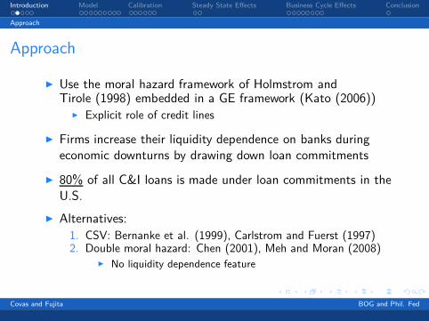
Use the moral hazard framework of Holmstrom andTirole (1998) embedded in a GE framework (Kato (2006))
Explicit role of credit lines
Firms increase their liquidity dependence on banks duringeconomic downturns by drawing down loan commitments
80% of all C&I loans is made under loan commitments in theU.S.
Alternatives:
1. CSV: Bernanke et al. (1999), Carlstrom and Fuerst (1997)2. Double moral hazard: Chen (2001), Meh and Moran (2008)
No liquidity dependence feature
Covas and Fujita BOG and Phil. Fed
Introduction Model Calibration Steady State Effects Business Cycle Effects Conclusion
Overview of the Paper
Main Idea
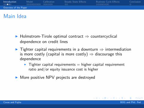
Holmstrom-Tirole optimal contract ⇒ countercyclicaldependence on credit lines
Tighter capital requirements in a downturn ⇒ intermediationis more costly (capital is more costly) ⇒ discourage thisdependence
Tighter capital requirements = higher capital requirementratio and/or equity issuance cost is higher
More positive NPV projects are destroyed
Covas and Fujita BOG and Phil. Fed
Introduction Model Calibration Steady State Effects Business Cycle Effects Conclusion
Overview of the Paper
Results
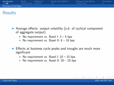
Average effects: output volatility (s.d. of cyclical componentof aggregate output)
No requirement vs. Basel I: 3 – 5 bps No requirement vs. Basel II: 8 – 10 bps
Effects at business cycle peaks and troughs are much moresignificant
No requirement vs. Basel I: 10 – 15 bps No requirement vs. Basel II: 20 – 25 bps
Covas and Fujita BOG and Phil. Fed

Introduction Model Calibration Steady State Effects Business Cycle Effects Conclusion
Outline
Outline
1. Model
2. Calibration
Utilization rate of credit lines Cyclical pressure on bank capital positions (Kashyap-Stein)
3. Steady state effects of permanently higher capital requirementratio from 8 to 12%
Transition dynamics
4. Business cycle effects Comparison of the three economies: (i) no regulation economy,
(ii) Basel I economy and (iii) Basel II economy
Covas and Fujita BOG and Phil. Fed
Introduction Model Calibration Steady State Effects Business Cycle Effects Conclusion
Environment
Model - Overview
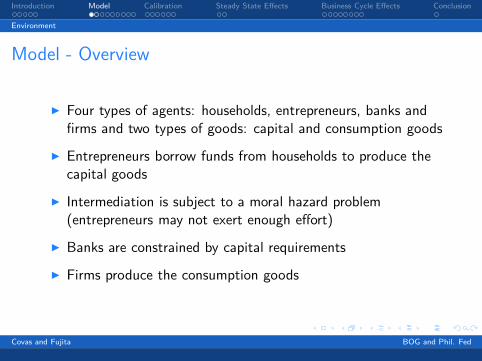
Four types of agents: households, entrepreneurs, banks andfirms and two types of goods: capital and consumption goods
Entrepreneurs borrow funds from households to produce thecapital goods
Intermediation is subject to a moral hazard problem(entrepreneurs may not exert enough effort)
Banks are constrained by capital requirements
Firms produce the consumption goods
Covas and Fujita BOG and Phil. Fed
Introduction Model Calibration Steady State Effects Business Cycle Effects Conclusion
Environment
Sequence of Events
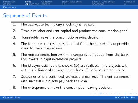
1. The aggregate technology shock (ǫ) is realized.
2. Firms hire labor and rent capital and produce the consumption good.
3. Households make the consumption-saving decision.
4. The bank uses the resources obtained from the households to provideloans to the entrepreneurs.
5. The entrepreneurs borrow i − n consumption goods from the bankand invests in capital-creation projects.
6. The idiosyncratic liquidity shocks (ω) are realized. The projects withω ≤ ω are financed through credit lines. Otherwise, are liquidated.
7. Outcomes of the continued projects are realized. The entrepreneurswith successful projects pay back the loan.
8. The entrepreneurs make the consumption-saving decision.
Covas and Fujita BOG and Phil. Fed
Introduction Model Calibration Steady State Effects Business Cycle Effects Conclusion
Financial Contract
Financial Contract (Intra Period)
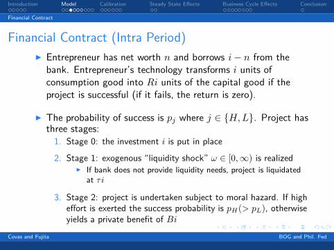
Entrepreneur has net worth n and borrows i− n from thebank. Entrepreneur’s technology transforms i units ofconsumption good into Ri units of the capital good if theproject is successful (if it fails, the return is zero).
The probability of success is pj where j ∈ H,L. Project hasthree stages:
1. Stage 0: the investment i is put in place
2. Stage 1: exogenous “liquidity shock” ω ∈ [0,∞) is realized If bank does not provide liquidity needs, project is liquidated
at τ i
3. Stage 2: project is undertaken subject to moral hazard. If higheffort is exerted the success probability is pH(> pL), otherwiseyields a private benefit of Bi
Covas and Fujita BOG and Phil. Fed
Introduction Model Calibration Steady State Effects Business Cycle Effects Conclusion
Financial Contract
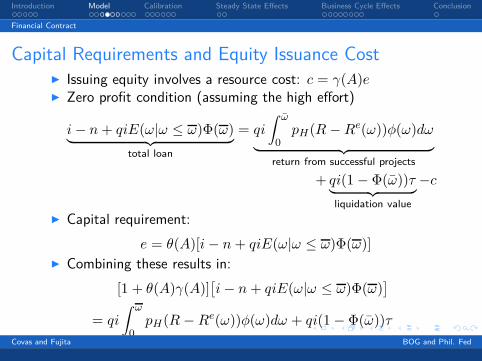
Capital Requirements and Equity Issuance Cost Issuing equity involves a resource cost: c = γ(A)e Zero profit condition (assuming the high effort)
i− n+ qiE(ω|ω ≤ ω)Φ(ω)︸ ︷︷ ︸
total loan
= qi
∫ ω
0
pH(R−Re(ω))φ(ω)dω︸ ︷︷ ︸
return from successful projects
+ qi(1− Φ(ω))τ︸ ︷︷ ︸
liquidation value
−c
Capital requirement:
e = θ(A)[i− n+ qiE(ω|ω ≤ ω)Φ(ω)]
Combining these results in:
[1 + θ(A)γ(A)][i− n+ qiE(ω|ω ≤ ω)Φ(ω)
]
= qi
∫ ω
0
pH(R −Re(ω))φ(ω)dω + qi(1− Φ(ω))τ
Covas and Fujita BOG and Phil. Fed
Introduction Model Calibration Steady State Effects Business Cycle Effects Conclusion
Financial Contract
Optimal Contract
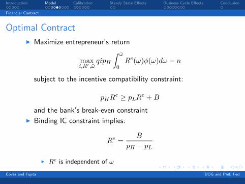
Maximize entrepreneur’s return
maxi,Re,ω
qipH
∫ ω
0
Re(ω)φ(ω)dω − n
subject to the incentive compatibility constraint:
pHRe ≥ pLR
e +B
and the bank’s break-even constraint
Binding IC constraint implies:
Re =B
pH − pL
Re is independent of ω
Covas and Fujita BOG and Phil. Fed

Introduction Model Calibration Steady State Effects Business Cycle Effects Conclusion
Financial Contract
Solution of the Financial Contract
Choose ω for given levels of n and q
FOC (when τ = 0):
q
∫ ω
0
Φ(ω)dω = 1
Zero profit condition implies:
i =1
1− qh(ω, θ(A)γ(A))n
where
h(ω, θ(A)γ(A)) =Φ(ω)pH
(R− B
pH−pL
)
1 + θ(A)γ(A)−E(ω|ω ≤ ω)Φ(ω)
Covas and Fujita BOG and Phil. Fed

Introduction Model Calibration Steady State Effects Business Cycle Effects Conclusion
Households
Households Representative household maximizes
E0
∞∑
t=0
βtu(ct, lt)
subject to
ct + st = rtkt +wt(1− lt)
kt+1 = (1− δ)kt +1
qtst
FOCs:
qt = βEt
(uc(ct+1, lt+1)
uc(ct, lt)
)[
rt+1 + (1− δ)qt+1
]
wt = −ul(ct, lt)
uc(ct, lt)Covas and Fujita BOG and Phil. Fed
Introduction Model Calibration Steady State Effects Business Cycle Effects Conclusion
Entrepreneurs
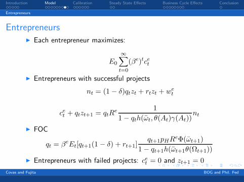
Entrepreneurs Each entrepreneur maximizes:
E0
∞∑
t=0
(βe)tcet
Entrepreneurs with successful projects
nt = (1− δ)qtzt + rtzt + wet
cet + qtzt+1 = qtRe 1
1− qth(ωt, θ(At)γ(At))nt
FOC
qt = βeEt[qt+1(1− δ) + rt+1]qt+1pHR
eΦ(ωt+1)
1− qt+1h(ωt+1θ(Ωt+1))
Entrepreneurs with failed projects: cet = 0 and zt+1 = 0
Covas and Fujita BOG and Phil. Fed

Introduction Model Calibration Steady State Effects Business Cycle Effects Conclusion
General Equilibrium
General Equilibrium Labor markets clearing:
Ht = (1− η)(1 − lt), Jt = η
Consumption goods market:
AtKαt HιtJ
1−α−ιt = (1− η)ct + ηcet + ηi
(
1 + qtE(ω|ω ≤ ω)Φ(ω)
+ qtθ(At)γ(At)Φ(ωt)ω0 − (1− Φ(ωt))τ
1 + θ(At)γ(At)
)
Capital goods:
Kt+1 = (1− δ)Kt + ηipHRΦ(ω)
Evolution of technology lnAt+1 = ρ lnAt + ǫt+1
Covas and Fujita BOG and Phil. Fed
Introduction Model Calibration Steady State Effects Business Cycle Effects Conclusion
Calibration
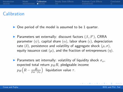
One period of the model is assumed to be 1 quarter.
Parameters set externally: discount factors (β, βe), CRRAparameter (ψ), capital share (α), labor share (ι), depreciationrate (δ), persistence and volatility of aggregate shock (ρ, σ),equity issuance cost (µ), and the fraction of entrepreneurs (η).
Parameters set internally: volatility of liquidity shock σω,expected total return pHR, pledgeable income
pH
(
R− BpH−pL
)
liquidation value τ .
Covas and Fujita BOG and Phil. Fed
Introduction Model Calibration Steady State Effects Business Cycle Effects Conclusion
Parameters Set Externally
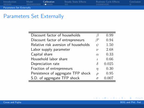
Parameters Set Externally
Discount factor of households β 0.99Discount factor of entrepreneurs βe 0.94Relative risk aversion of households ψ 1.50Labor supply parameter ν 2.68Capital share α 0.33Household labor share ι 0.66Depreciation rate δ 0.025Fraction of entrepreneurs η 0.30Persistence of aggregate TFP shock ρ 0.95S.D. of aggregate TFP shock σ 0.007
Covas and Fujita BOG and Phil. Fed
Introduction Model Calibration Steady State Effects Business Cycle Effects Conclusion
Parameters Set Internally
Parameters Set Internally
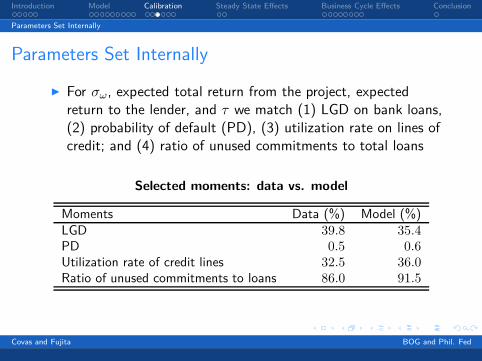
For σω, expected total return from the project, expectedreturn to the lender, and τ we match (1) LGD on bank loans,(2) probability of default (PD), (3) utilization rate on lines ofcredit; and (4) ratio of unused commitments to total loans
Selected moments: data vs. model
Moments Data (%) Model (%)LGD 39.8 35.4PD 0.5 0.6Utilization rate of credit lines 32.5 36.0Ratio of unused commitments to loans 86.0 91.5
Covas and Fujita BOG and Phil. Fed
Introduction Model Calibration Steady State Effects Business Cycle Effects Conclusion
Capital Requirements and Equity Issuance Cost
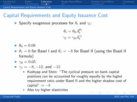
Capital Requirements and Equity Issuance Cost
Specify exogenous processes for θt and γt:
θt = θ0Aθ1t
γt = γ0Aγ1t
θ0 = 0.08
θ1 = 0 for Basel I and θ1 = −8 for Basel II (using the Basel IIformula)
γ0 = 0.05 γ1 = −8,−12, and −15
Kashyap and Stein: “The cyclical pressure on bank capitalpositions can be accounted for roughly equally by the higherrequirement ratio under Basel II and the higher shadow cost ofcapital” ⇒ −8
Also try higher elasticities
Covas and Fujita BOG and Phil. Fed

Introduction Model Calibration Steady State Effects Business Cycle Effects Conclusion
Sample Paths
Sample Paths
1400 1410 1420 1430 1440 1450 1460
5
6
7
8
9
10
11
12
(%)
Time periods
1400 1410 1420 1430 1440 1450 14600.84
0.86
0.88
0.9
0.92
0.94
0.96
0.98Cap requirementsEquity issuance costOutput
Covas and Fujita BOG and Phil. Fed

Introduction Model Calibration Steady State Effects Business Cycle Effects Conclusion
Sample Paths
Sample Paths (Equity Issuance Cost)
1400 1410 1420 1430 1440 1450 14602
3
4
5
6
7
8
9
10
11
Time Period
(%)
γ1=−8
γ1=−12
γ1=−15
Covas and Fujita BOG and Phil. Fed

Introduction Model Calibration Steady State Effects Business Cycle Effects Conclusion
Experiment
Steady-State Experiment
Consider an experiment: the capital requirement ratio 8% to12%
Other variables (incl. equity issuance cost) are kept constant
Covas and Fujita BOG and Phil. Fed
Introduction Model Calibration Steady State Effects Business Cycle Effects Conclusion
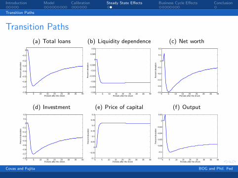
Transition Paths
Transition Paths
(a) Total loans
0 5 10 15 20 25 30 35 40−0.8
−0.7
−0.6
−0.5
−0.4
−0.3
−0.2
−0.1
0
Per
cent
dev
iatio
n
Periods after the shock
(b) Liquidity dependence
0 5 10 15 20 25 30 35 40−0.03
−0.025
−0.02
−0.015
−0.01
−0.005
0
0.005
0.01
Per
cent
dev
iatio
n
Periods after the shock
(c) Net worth
0 5 10 15 20 25 30 35 40−0.5
−0.4
−0.3
−0.2
−0.1
0
0.1
0.2
Per
cent
dev
iatio
n
Periods after the shock
(d) Investment
0 5 10 15 20 25 30 35 40−0.8
−0.7
−0.6
−0.5
−0.4
−0.3
−0.2
−0.1
0
0.1
0.2
Per
cent
dev
iatio
n
Periods after the shock
(e) Price of capital
0 5 10 15 20 25 30 35 40−0.1
−0.05
0
0.05
0.1
0.15
0.2
0.25
0.3
Per
cent
dev
iatio
n
Periods after the shock
(f) Output
0 5 10 15 20 25 30 35 40−0.12
−0.1
−0.08
−0.06
−0.04
−0.02
0
0.02
Per
cent
dev
iatio
n
Periods after the shock
Figure:
Covas and Fujita BOG and Phil. Fed

Introduction Model Calibration Steady State Effects Business Cycle Effects Conclusion
Exercises
Exercises
1. Temporary increase in the capital requirement ratio θ increases from 0.08 to 0.10 on impact and gradually returns
to 0.08
2. Responses to the aggregate shock in the economy with nocapital requirement
3. Compare responses in the (i) no requirement economy, (ii)Basel I economy, and (iii) Basel II economy
Basel I: only equity issuance cost is time varying
Basel II: both equity issuance cost and capital requirement aretime varying
Covas and Fujita BOG and Phil. Fed

Introduction Model Calibration Steady State Effects Business Cycle Effects Conclusion
Capital Requirement Shock
A Temporary Increase in Capital Requirement
(a) Total loans
0 5 10 15 20 25 30
−0.5
−0.4
−0.3
−0.2
−0.1
0
Per
cent
dev
iatio
n
Periods after the shock
(b) Liquidity dependence
0 5 10 15 20 25 30−10
−9
−8
−7
−6
−5
−4
−3
−2
−1
0
1x 10
−3
Per
cent
dev
iatio
n
Periods after the shock
(c) Net worth
0 5 10 15 20 25 30−0.45
−0.4
−0.35
−0.3
−0.25
−0.2
−0.15
−0.1
−0.05
0
0.05
Per
cent
dev
iatio
n
Periods after the shock
(d) Investment
0 5 10 15 20 25 30
−0.5
−0.4
−0.3
−0.2
−0.1
0
Per
cent
dev
iatio
n
Periods after the shock
(e) Price of capital
0 5 10 15 20 25 30−0.01
0
0.01
0.02
0.03
0.04
0.05
0.06
0.07
0.08
0.09
Per
cent
dev
iatio
n
Periods after the shock
(f) Output
0 5 10 15 20 25 30−0.1
−0.09
−0.08
−0.07
−0.06
−0.05
−0.04
−0.03
−0.02
−0.01
0
0.01
Per
cent
dev
iatio
n
Periods after the shock
Figure:
Covas and Fujita BOG and Phil. Fed

Introduction Model Calibration Steady State Effects Business Cycle Effects Conclusion
TFP Shock
A Negative TFP Shock (No Capital Requirement)
(a) Total loans
0 5 10 15 20 25 30−4
−3.5
−3
−2.5
−2
−1.5
−1
−0.5
0
Per
cent
dev
iatio
n
Periods after the shock
(b) Liquidity dependence
0 5 10 15 20 25 30−0.01
0
0.01
0.02
0.03
0.04
0.05
Per
cent
dev
iatio
n
Periods after the shock
(c) Net worth
0 5 10 15 20 25 30−4
−3.5
−3
−2.5
−2
−1.5
−1
−0.5
0
Per
cent
dev
iatio
n
Periods after the shock
(d) Investment
0 5 10 15 20 25 30−4
−3.5
−3
−2.5
−2
−1.5
−1
−0.5
0
Per
cent
dev
iatio
n
Periods after the shock
(e) Price of capital
0 5 10 15 20 25 30−0.5
−0.45
−0.4
−0.35
−0.3
−0.25
−0.2
−0.15
−0.1
−0.05
0
0.05
Per
cent
dev
iatio
n
Periods after the shock
(f) Output
0 5 10 15 20 25 30
−1
−0.8
−0.6
−0.4
−0.2
0
Per
cent
dev
iatio
n
Periods after the shock
Figure:
Covas and Fujita BOG and Phil. Fed

Introduction Model Calibration Steady State Effects Business Cycle Effects Conclusion
Comparison Across Different Regulatory Environments
Responses Under Different Environments
(a) Total loans
0 5 10 15 20 25 30−4
−3.5
−3
−2.5
−2
−1.5
−1
−0.5
0
Periods after the shock
Per
cent
dev
iatio
n
BenchmarkBasel IBasel II
(b) Liquidity dependence
0 5 10 15 20 25 30−0.01
0
0.01
0.02
0.03
0.04
0.05
Per
cent
dev
iatio
n
Periods after the shock
(c) Net worth
0 5 10 15 20 25 30−4
−3.5
−3
−2.5
−2
−1.5
−1
−0.5
0
Per
cent
dev
iatio
n
Periods after the shock
(d) Investment
0 5 10 15 20 25 30−4
−3.5
−3
−2.5
−2
−1.5
−1
−0.5
0
Per
cent
dev
iatio
n
Periods after the shock
(e) Price of capital
0 5 10 15 20 25 30−0.45
−0.4
−0.35
−0.3
−0.25
−0.2
−0.15
−0.1
−0.05
0
0.05
Per
cent
dev
iatio
n
Periods after the shock
(f) Output
0 5 10 15 20 25 30
−1
−0.8
−0.6
−0.4
−0.2
0
Per
cent
dev
iatio
n
Periods after the shock
Figure:
Covas and Fujita BOG and Phil. Fed

Introduction Model Calibration Steady State Effects Business Cycle Effects Conclusion
Output Volatility
Output Volatility
Table: Standard Deviations
No Requirement Basel I Basel II
Baseline (γ1 = −8)1.84 1.87 1.92— (1.016) (1.043)
γ1 = −12— 1.89 1.94— (1.027) (1.054)
γ1 = −15— 1.91 1.97— (1.038) (1.071)
Notes: Results are based on 500 replications of 200 observations (afterrandomization of the initial condition). The standard deviations are basedon logged HP-filtered series with a smoothing parameter of 1,600. Num-bers in parentheses report relative volatilities compared to that under theeconomy with no capital requirement.
Covas and Fujita BOG and Phil. Fed
Introduction Model Calibration Steady State Effects Business Cycle Effects Conclusion
Effects in Booms and Recessions
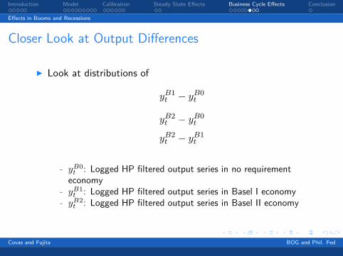
Closer Look at Output Differences
Look at distributions of
yB1t − y
B0t
yB2t − y
B0t
yB2t − y
B1t
- yB0
t : Logged HP filtered output series in no requirementeconomy
- yB1
t: Logged HP filtered output series in Basel I economy
- yB2
t : Logged HP filtered output series in Basel II economy
Covas and Fujita BOG and Phil. Fed

Introduction Model Calibration Steady State Effects Business Cycle Effects Conclusion
Effects in Booms and Recessions
Sample Paths of Differences in Output (γ1 = −8)
1000 1020 1040 1060 1080 1100 1120 1140 1160 1180 1200−0.3
−0.25
−0.2
−0.15
−0.1
−0.05
0
0.05
0.1
0.15
0.2
quarterly data
perc
enta
ge d
iffer
ence
(ytB1−y
tB0)100
(ytB2−y
tB0)100
Covas and Fujita BOG and Phil. Fed

Introduction Model Calibration Steady State Effects Business Cycle Effects Conclusion
Effects in Booms and Recessions
Distribution of Output Differences
Table: Percentiles
Percentiles 1 5 95 99
(yB1
t− yB0
t)100 −0.12 −0.08 0.06 0.09
Baseline (yB2
t − yB0
t )100 −0.40 −0.18 0.15 0.25
(yB2
t− yB1
t)100 −0.27 −0.11 0.09 0.17
(yB1
t− yB0
t)100 −0.22 −0.12 0.10 0.15
γ1 = −12 (yB2
t − yB0
t )100 −0.61 −0.24 0.20 0.38
(yB2
t− yB1
t)100 −0.39 −0.13 0.11 0.25
(yB1
t− yB0
t)100 −0.32 −0.16 0.13 0.21
γ1 = −15 (yB2
t − yB0
t )100 −0.83 −0.30 0.25 0.53
(yB2
t− yB1
t)100 −0.51 −0.14 0.14 0.34
Covas and Fujita BOG and Phil. Fed
Introduction Model Calibration Steady State Effects Business Cycle Effects Conclusion
Conclusion
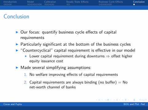
Our focus: quantify business cycle effects of capitalrequirements
Particularly significant at the bottom of the business cycles
“Countercyclical” capital requirement is effective in our model Lower capital requirement during downturns ⇒ offset higher
equity issuance cost
Made several simplifying assumptions:
1. No welfare improving effects of capital requirements
2. Capital requirements are always binding (no buffer) = Nonet-worth channel of banks
Covas and Fujita BOG and Phil. Fed