1

Processing scanner data in the Dutch CPI:

A new methodology and first experiences1

Antonio G. Chessa2

1 The author wants to thank his colleagues for their continuous support and discussions. The views expressed in this

paper are those of the author and do not necessarily reflect the policies of Statistics Netherlands. 2 Statistics Netherlands, Team CPI; P.O. Box 24500, 2490 HA The Hague, The Netherlands. E-mail: ag.chessa@cbs.nl

2

Abstract This paper presents a new methodology for processing electronic transaction data and for calculating price indices, with the aim of reducing the differences across the methods used for different retailers and consumer goods in the Dutch CPI. Meaningful price indices can only be computed when products are homogeneous. GTINs (barcodes) contain the highest degree of homogeneity. However, their use may be hampered by the occurrence of so-called “relaunches”, which refers to barcode changes of items that are repositioned in the market. The former and new GTINs need to be linked in order to capture possible price increases. This may be achieved through retailers’ own product codes (Stock Keeping Units), or otherwise through item characteristics. A sensitivity analysis is proposed for selecting item attributes, which quantifies the additional impact of attributes on price change. The selection procedure can be combined with the expertise of consumer specialists. The new index method calculates price indices as a ratio of a turnover index and a weighted quantity index. The method is in fact the Geary-Khamis method applied to the time domain. Quantity weights of homogeneous products are calculated from prices and quantities of each month in the year of publication. The weights are updated each month, which are used to calculate direct indices with respect to the base month. The method does not lead to chain drift as the price indices coincide with the transitive version of the method at the end of each year. Comparisons with two variants of the method suggest that the substitution bias is negligible. The new methodology has replaced the current sample-based method in the CPI for mobile phones in January 2016. The paper concludes with some first experiences with the method. Keywords: CPI, scanner data, GTIN, relaunch, product homogeneity, index theory, transitivity, substitution bias.

3

1. Introduction

Scanner data have clear advantages over traditional survey data collection, notably

because such data sets offer a better coverage of items sold, they contain complete

transaction information (prices and quantities), and the data collection process is

automatised. In spite of their potential, scanner data are still used by a small number of

statistical agencies in their CPI, but the number is likely to increase in the coming years.3

By scanner data we mean transaction data that specify turnover and numbers of

items sold by GTIN (barcode). At the time of introduction in the Dutch CPI in 2002,

scanner data involved two supermarket chains. In January 2010, the data were extended

to six supermarket chains, as part of a re-design of the CPI (de Haan, 2006; van der Grient

and de Haan, 2010; de Haan and van der Grient, 2011). At present, scanner data of 10

supermarket chains are used and surveys are not carried out anymore for supermarkets

since January 2013. Also scanner data from other retailers are received and used in the

CPI. Other forms of electronic data containing both price and quantity information are

obtained from travel agencies, for fuel prices and for mobile phones. More than 20% of the

Dutch CPI is based on electronic transaction data (in terms of Coicop weights of 2015).

The shift from traditional price collection to electronic transaction data has

introduced new possibilities for developing index methods. Ideally, we would like to

develop a method that makes use of both prices and quantities, and that processes the

transactions of all GTINs instead of taking a sample.4 With thousands of GTINs per retailer

the question is how to find efficient and satisfactory solutions. This has turned out to be a

complex process over the years, which is reflected in the range of different methods across

retailers and consumer goods in the Dutch CPI (Walschots, 2016). The current method for

supermarket scanner data intends to process all GTINs, while the methods for other

retailers still make use of samples of items.

As the search for new electronic data continues, the question has been put forward

whether a generic index method could be developed that is applicable to different types of

consumer goods and that is capable of handling issues that are not resolved in a fully

satisfactory way so far in certain methods (amongst which the “relaunch” problem and,

related to this, the definition of homogeneous products). Such a method could then also be

gradually applied to data sets that are currently in production.

Section 2 gives a global outline of a new methodology for processing electronic

transaction data. The intention of this section is to show how the new methodology fits

within the CPI system. The aim of the methodology is twofold: (1) to process all GTINs,

thus abandoning the traditional approach of selecting a basket of goods, and (2) to have an

index method that deals with the dynamics of an assortment over time, in which new

goods are timely included, and that efficiently handles relaunches.

Sections 3 and 4 elaborate the two essential components of the new methodology:

product homogeneity and price index calculation. The relaunch problem implies that

GTINs are not always appropriate as unique identifiers of homogeneous products. Product

homogeneity should then be achieved at a broader level, at which GTINs are combined

into groups. Homogeneous products could be defined by combining GTINs that share the

3 In Europe, six countries will be using scanner data in 2016. The scanner data workshops in Vienna (2014) and

Rome (2015) evidenced that several countries are expecting their first data, while other countries made concrete steps towards acquiring their first scanner data. 4 In this paper, the term “item” and GTIN are used interchangeably.

4

same set of characteristics. These have to be selected in some way. Section 3 describes and

illustrates a method for this purpose.

Turnover and quantities sold of items are summed and used to calculate unit values

for each homogeneous product. These are used to calculate price indices for, what is called

here “consumption segments”, which consist of one or more homogeneous products (e.g.,

a segment T-shirts with products that are described by one or more characteristics). The

index method that has been developed for this purpose is described in Section 4.

The price index method uses prices and quantities of each month in the publication

year for calculating and monthly updating product weights. This means that relatively

little information is used in the first publication months (two months in January, three in

February, etc., with December as base month). This could make price indices more volatile

than in later months. In order to investigate this, price indices are compared with a

transitive version of the method, which uses all 13 months for calculating the indices of

each month. The results of an extensive empirical study are presented in Section 5.2.

A second issue concerns the weighting scheme used for calculating the quantity

weights of the products. The product prices of each month are deflated by the price indices

and weighted according to the share of the quantities sold in a month. The Geary-Khamis

method has been the subject of criticism in international price comparisons, as the

commodity prices of large countries receive higher (quantity based) weights than those of

smaller countries. If the larger countries exhibit higher prices, then a situation arises that

is felt to contradict with economic theories (consumers tend to buy more when prices

decrease). This effect is known as the Gerschenkron effect and could also apply to

intertemporal comparisons (where it is known as the “substitution effect”). Two variants

of the index method with alternative weighting schemes are therefore investigated and

compared with the base method. The results are presented in Section 5.3.

Section 6 summarises the first experiences with the methodology in the Dutch CPI for

mobile phones. Final remarks are made in Section 7.

2. Outline of a new processing framework

The introduction of different methods for different retailers in the Dutch CPI has made the

system increasingly complex over time. New choices were made each time a new data set

was added to the production system. The current index method for supermarkets makes

use of different types of price and turnover filters. A Jevons index is used for elementary

aggregates (“consumption segments”). Because of the equal weighting of GTINs

(homogeneous products), items with monthly turnover shares below a certain threshold

are excluded. Old and new GTINs of relaunched items are not linked. A “dump price filter”

is applied to outgoing GTINs in order to limit downward biases of the index. The methods

for non-supermarkets make use of samples in order to have more grip on the relaunch

problem. On the other hand, these methods need continuous monitoring as the turnover of

samples of goods may decrease due to assortment changes.

For these reasons, the possibilities of developing a generic method have been studied

in order to reduce the current methodological differences in the Dutch CPI. The new

methodology focuses on three sources of methodological differences:

Data processing. The new methodology aims at integral data processing, thus

abandoning the traditional idea of calculating price indices for baskets of goods.

5

Increased assortment changes and dynamics need to be accommodated into an index

method.

Product differentiation and homogeneity.

In principle, the GTIN level is the most detailed level of homogeneity. This level can be

chosen for defining individual products in cases where relaunches do not occur.

Otherwise, a less detailed level of product differentiation is needed in order to link

GTINs of relaunched items. Possibilities for achieving this are described in the next

section.

Price index calculation.

The quest is for an index method that allows processing all transactions, which

involves timely inclusion of new items in the course of a publication year.

A summary is now given of how the new methodology is being integrated into the CPI

production system. The processing of electronic data in the Dutch CPI can roughly be

subdivided into four stages:

1. Reading and checking data;

2. Linking items/GTINs to Coicops;

3. Calculating prices and price indices for “lower aggregate levels”;

4. Calculating price indices for Coicops and for the overall CPI.

The first stage consists of reading data files and performing basic checks on the data, such

as the correctness and completeness of records and record variables and controlling for

quantities sold with value zero (which are isolated before item prices are calculated). The

subsequent three steps are worked out in more detail in the chart of Figure 1. The “lower

aggregate levels” mentioned in step 3 consist of three levels, which are explained below.

Item group levels

Consumer goods and services are subdivided in the CPI into Coicops. The most detailed

level of publication within Coicop divisions is referred to as “L-Coicop” in the Dutch CPI.5

Scanner data contain transaction data at GTIN level. Further subdivisions are made

between L-Coicop and GTIN level. Individual GTINs may have to be combined into groups,

which we refer to as “homogeneous products”. These products and their underlying items

need to be linked to L-Coicops. In order to do this efficiently, it is important to ask retailers

for their own classification of GTINs (called “ESBAs” in our system).

Usually, we take the most detailed ESBA level for establishing the GTIN-Coicop links.

However, the most detailed ESBAs may still cover more than one L-Coicop, so that we

need to define an intermediate level between L-Coicops and homogeneous products. This

intermediate level, which we call “consumption segments”, may be derived from more

detailed GTIN characteristics (more details are given in the next section). In our

implementation of the methodology, consumption segments represent item types, such as

men’s T-shirts, men’s socks, mobile phones and chocolate. Each of these segments contains

a set of homogeneous products. For T-shirts, a product may contain GTINs that have the

same number of items per package, the same sleeve length, fabric and colour. In this way

we obtain a nested partition of individual items/GTINs at different levels, as is shown in

Figure 1.

5 L-Coicops are specified at the fifth digit level at most (depending on Coicop division).

6

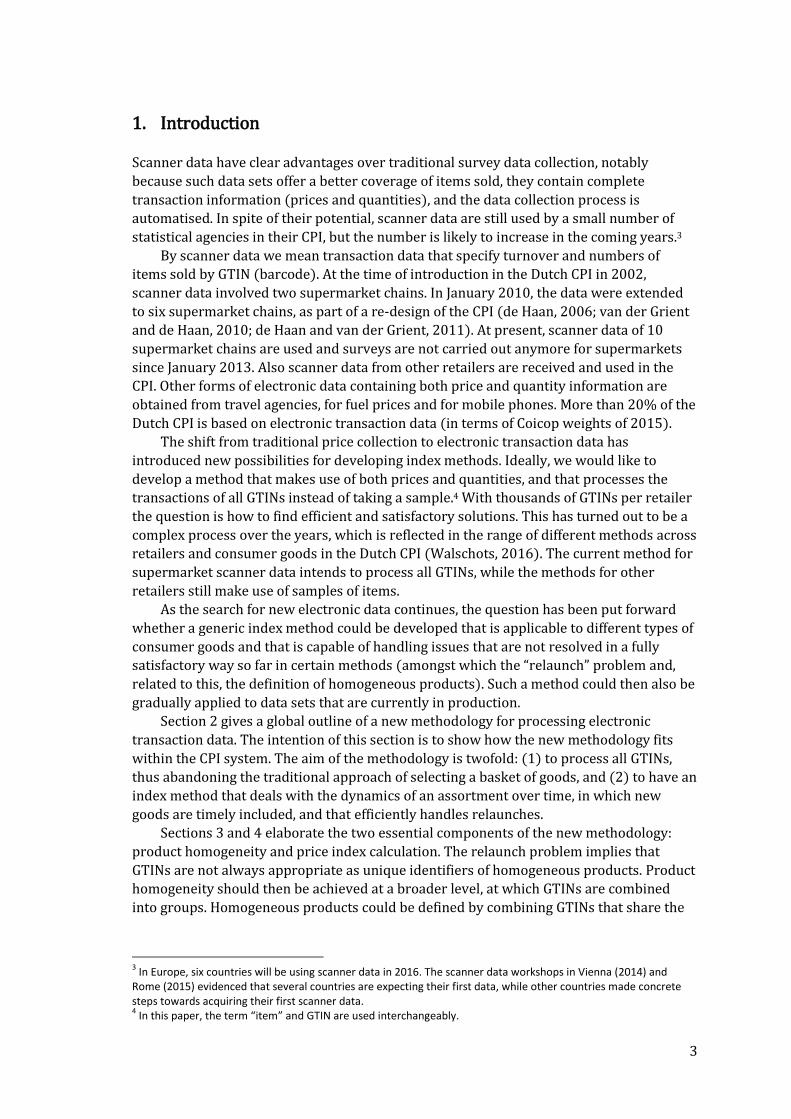
Figure 1. Nested group levels of individual items in the CPI, and price definitions and price index calculations at these levels in the new methodology.

Calculation of price indices

At each level in Figure 1 we either need to define prices or establish the method for

calculating price indices. The price of an individual item is its “transaction price”, that is,

turnover divided by number of items sold (in fact, this is a unit value at GTIN level). The

same holds for homogeneous products. Turnover and quantities sold are summed over

items that belong to the same product; their ratio yields a unit value.

Unit values and quantities sold for homogeneous products are subsequently used to

calculate a price index for each consumption segment. An index method is developed for

this purpose, referred to as the “QU-method”, which is described in Section 4. Price indices

for consumption segments are then aggregated to L-Coicops and higher levels according to

Laspeyres type indices, with weights based on turnover of the preceding year.6

3. Consumption segments and product homogeneity

In order to make choices about consumption segments and homogeneous products,

statistical agencies should ask retailers for information about item characteristics and

item classifications used by retailers for their own purpose (ESBAs). Information about

item characteristics may be contained in item descriptions and also in detailed ESBAs. Our

experiences with electronic data sets show that this information may be supplied in

varying formats by different retailers. For instance, the record variables in drugstore

6 Aggregation to Coicop levels could also be carried out by applying the aggregation according to the QU-method, by

summing turnover and weighted quantities in the numerator and the denominator of index formula (1) over consumption segments (see Section 4.1). Preliminary research showed negligible differences between the two aggregation methods at L-Coicop level.

(L-)Coicops

Consumption segments

Homogeneous products

Individual items/GTINs

Laspeyres type indices

QU-indices

Product prices (unit values)

Item transaction prices

Retailer's ESBAs

Item groups Index calculation

Men's T-shirts

#items, fabric, colour, sleeve

length

GTINs for men's T-shirts

Example

L-Coicop Menswear

7

scanner data are all contained in separate columns (Chessa, 2013). But information about

item characteristics may also be exclusively contained in text strings of GTIN descriptions.

The first example is clearly the preferred data format, as consumption segments and

products can be derived immediately, and GTINs can be automatically assigned to both

item group levels and linked to Coicop. In the second case, some form of text mining will

have to be applied in order to retrieve and place information about item characteristics in

separate columns. Text mining falls outside the scope of this paper and will therefore not

be treated further.

Consumption segments are defined as sets of homogeneous products. In our

experiments with the new methodology so far, consumption segments are defined as

‘types of item’. Item types can be defined at different levels of detail (e.g., different types of

socks combined into one segment, or sports, thermal and walking socks as separate

segments). After first tests with department store scanner data, we have decided to define

consumption segments at a broad item type level (i.e., sports, thermal and walking socks

for men combined into one segment “men’s socks”). We expect that this choice requires

less monthly system maintenance than the more detailed segment definition and also less

index imputations.

When consumption segments have been defined, the question is how to define

homogeneous products. Before proceeding, we introduce the following terminology. By

“characteristic” of an item we refer to an instance, a specific value that an item can take.

Such a value belongs to a broader set or class, which we refer to as “attribute”. For

example, ‘white’ is a characteristic of a T-shirt that belongs to the attribute ‘colour’.

The relaunch problem plays a crucial part in selecting the eventual approach for

defining products. The strategy could be roughly divided into the following stages:

1. If relaunches do not occur in a specific type of assortment, then GTINs are a natural

choice for homogeneous products.

2. If relaunches do occur, then a broader level of product differentiation is needed in

order to combine different GTINs into the same group. A data set should contain

additional information about items beside GTIN codes, turnover and quantities sold in

order to establish GTIN matches. The following possibilities can be thought of:

a. old and new GTINs could be matched through the retailer’s internal product codes

or SKUs (Stock Keeping Units). Retailers usually assign the same SKUs to items

which replace goods on the shelves that leave the assortment;

b. if SKUs are not available, or cannot be used for some reason, then different GTINs

can be matched when they share the same item characteristics.

How to proceed under situations 1 and 2a should be obvious. Once a choice for either

GTINs or SKUs is made the products are defined, so that price indices can be calculated.

Situation 2b needs to be elaborated. The central question is which characteristics should

be selected and what approach could be used for this purpose. Before we proceed with

this, some examples are given that illustrate the appropriateness (or not) of GTINs for

differentiating products.

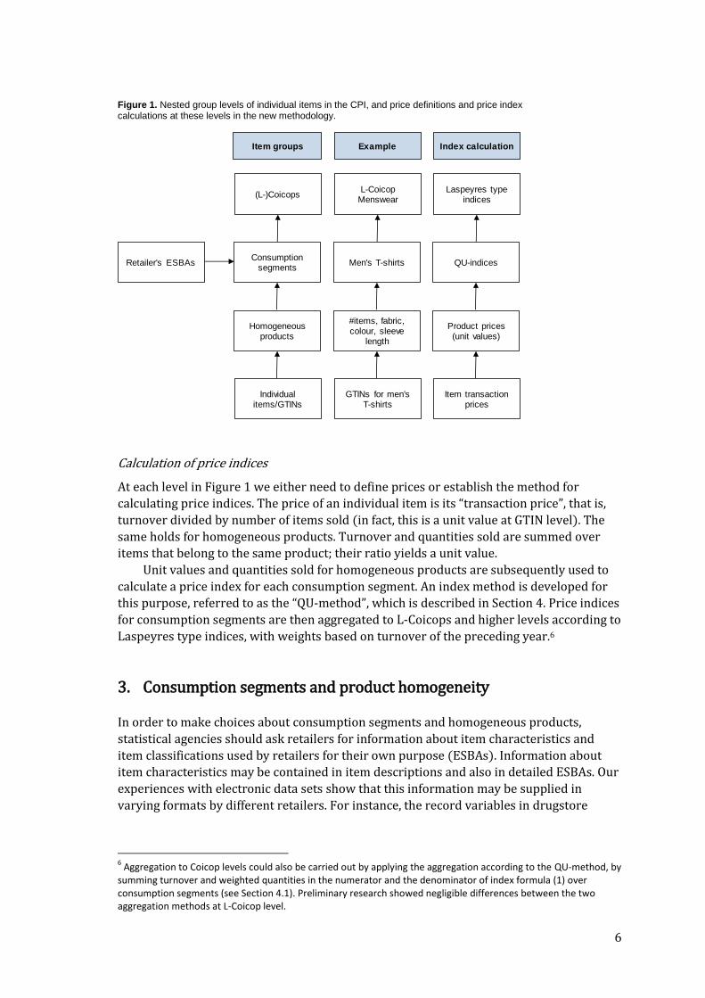
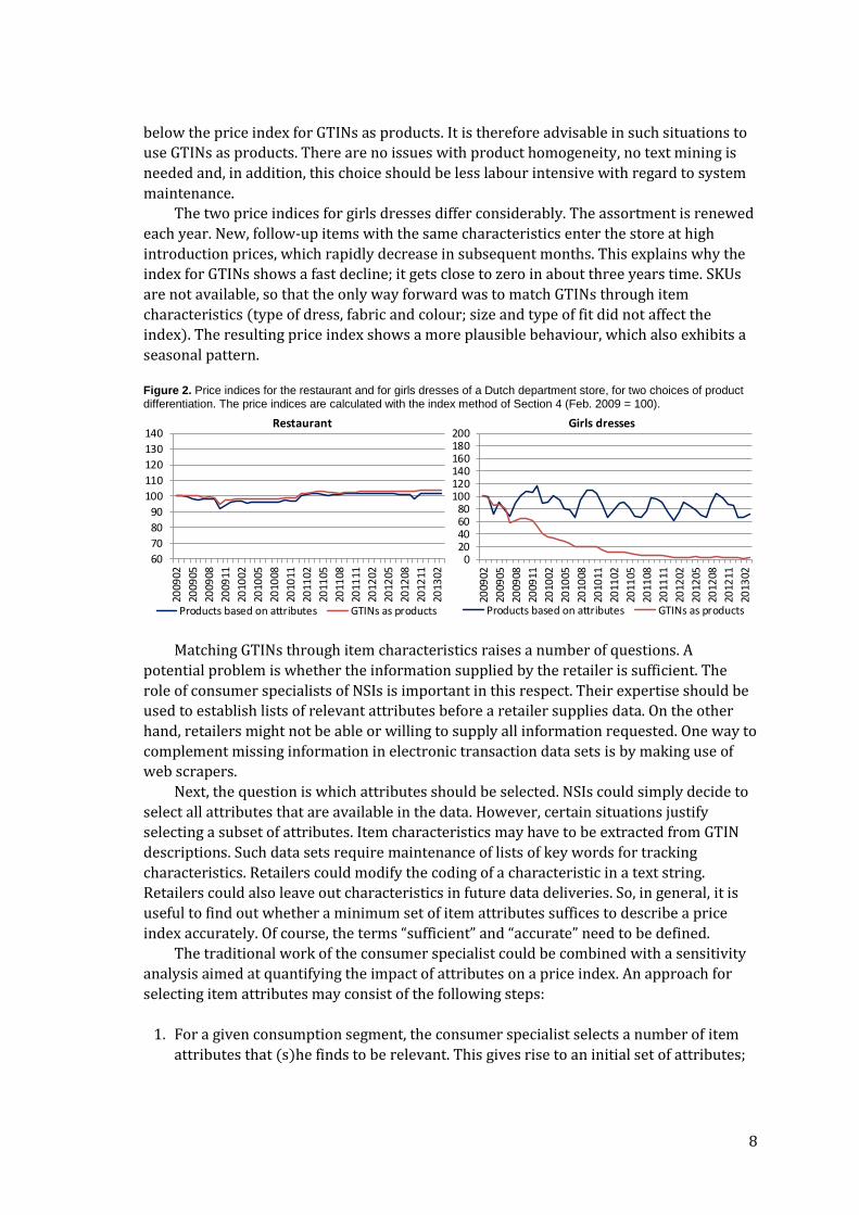
Figure 2 shows price indices at two levels of product differentiation for the restaurant

services and for girls dresses of a Dutch department store. The assortment of the

restaurant is stable over time. As a consequence, calculating price indices with GTINs as

products does not lead to problems. Product differentiation according to a limited set of

attributes (type of meal or drink, size and taste) gives a price index that even lies a bit

8

below the price index for GTINs as products. It is therefore advisable in such situations to

use GTINs as products. There are no issues with product homogeneity, no text mining is

needed and, in addition, this choice should be less labour intensive with regard to system

maintenance.

The two price indices for girls dresses differ considerably. The assortment is renewed

each year. New, follow-up items with the same characteristics enter the store at high

introduction prices, which rapidly decrease in subsequent months. This explains why the

index for GTINs shows a fast decline; it gets close to zero in about three years time. SKUs

are not available, so that the only way forward was to match GTINs through item

characteristics (type of dress, fabric and colour; size and type of fit did not affect the

index). The resulting price index shows a more plausible behaviour, which also exhibits a

seasonal pattern.

Figure 2. Price indices for the restaurant and for girls dresses of a Dutch department store, for two choices of product differentiation. The price indices are calculated with the index method of Section 4 (Feb. 2009 = 100).

Matching GTINs through item characteristics raises a number of questions. A

potential problem is whether the information supplied by the retailer is sufficient. The

role of consumer specialists of NSIs is important in this respect. Their expertise should be

used to establish lists of relevant attributes before a retailer supplies data. On the other

hand, retailers might not be able or willing to supply all information requested. One way to

complement missing information in electronic transaction data sets is by making use of

web scrapers.

Next, the question is which attributes should be selected. NSIs could simply decide to

select all attributes that are available in the data. However, certain situations justify

selecting a subset of attributes. Item characteristics may have to be extracted from GTIN

descriptions. Such data sets require maintenance of lists of key words for tracking

characteristics. Retailers could modify the coding of a characteristic in a text string.

Retailers could also leave out characteristics in future data deliveries. So, in general, it is

useful to find out whether a minimum set of item attributes suffices to describe a price

index accurately. Of course, the terms “sufficient” and “accurate” need to be defined.

The traditional work of the consumer specialist could be combined with a sensitivity

analysis aimed at quantifying the impact of attributes on a price index. An approach for

selecting item attributes may consist of the following steps:

1. For a given consumption segment, the consumer specialist selects a number of item

attributes that (s)he finds to be relevant. This gives rise to an initial set of attributes;

60

70

80

90

100

110

120

130

140

2009

02

2009

05

2009

08

2009

11

2010

02

2010

05

2010

08

2010

11

2011

02

2011

05

2011

08

2011

11

2012

02

2012

05

2012

08

2012

11

2013

02Restaurant

Products based on attributes GTINs as products

020406080

100120140160180200

2009

02

2009

05

2009

08

2009

11

2010

02

2010

05

2010

08

2010

11

2011

02

2011

05

2011

08

2011

11

2012

02

2012

05

2012

08

2012

11

2013

02

Girls dresses

Products based on attributes GTINs as products

9

2. A price index is calculated for the consumption segment according to the method of

Section 4. GTINs that share the same characteristics, which are chosen in step 1, are

combined into the same product;

3. A sensitivity analysis is performed: an attribute that was not selected in step 1 is now

added and the price index is re-calculated. If the price index changes “significantly”,

then the attribute is added. This step can be repeated with other attributes. Attributes

may also be omitted when their impact on the price index is negligible.

An example of a sensitivity analysis is given below.

The new methodology is being tested on scanner data of the Dutch department store

referred to previously in this paper. Text mining was applied to this data set in order to

extract item characteristics from the GTIN descriptions. This is done for consumption

segments where relaunches occur, in particular clothing (see Figure 2). Food and non-

alcoholic beverages (Coicop 01) and the restaurant services (Coicop 11) are differentiated

by taking GTINs as homogeneous products. Consequently, text mining was not required

for these two Coicops (at least, so far).

Lists of key words have been set up for each item characteristic in order to search

through the GTIN descriptions. Historical data from the period February 2009 until March

2013 were initially used for this purpose (which now has been extended in order to

prepare the methodology for the CPI). This example covers the four-year period for

illustrational purposes.

The selection of item attributes is illustrated for men’s and ladies’ wear. These two L-

Coicops are subdivided into four and eight consumption segments, respectively, for the

department store:

Men’s wear: socks, underwear, T-shirts, and sweaters and pullovers;

Ladies’ wear: socks, stockings, tights, nightwear, bras, underwear, T-shirts, and

sweaters and pullovers.

The consumer specialist selected the following item attributes (step 1):

Type of garment;

Number of items in a package;

Fabric;

Seasonality (e.g., sleeve length);

Colour.

Some attributes only apply to specific consumption segments (e.g., seasonality applies to

T-shirts, pullovers and tights, but not to nightwear and bras).

Price indices were calculated for products differentiated by the above list of

attributes. The index method of Section 4 was applied to each consumption segment.

These price indices were subsequently aggregated to L-Coicop by calculating Laspeyres

type indices, with the turnover shares of the consumption segments of the preceding year

serving as weights. The approach illustrated in Figure 1 was thus used.

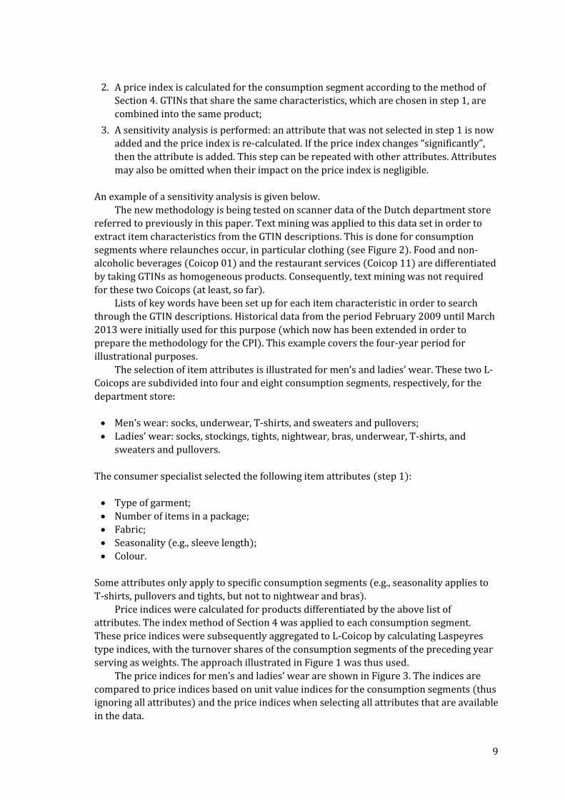
The price indices for men’s and ladies’ wear are shown in Figure 3. The indices are

compared to price indices based on unit value indices for the consumption segments (thus

ignoring all attributes) and the price indices when selecting all attributes that are available

in the data.

10

Figure 3. Price indices for men’s and ladies’ wear of the department store, compared with unit value based indices and price indices when all attributes are selected (Feb. 2009 = 100).

The price indices that are based on the attributes selected by the consumer specialist

(dark blue lines in Figure 3) are found to be satisfactory. The differences with the price

indices when all attributes would be selected (light blue lines) are small at L-Coicop level

and can be ignored at overall CPI level. The differences between the year-on-year price

indices would affect the CPI by slightly more than 0.001 percentage point in 2010 and

even less than 0.001 percentage point in 2011 and 2012. Fabric and colour could even be

omitted without altering these findings.

Men’s and ladies’ wear make up about 25 per cent of the weight of the department

store in the Dutch CPI. Products are differentiated at GTIN level for Coicops 01 and 11, so

there is no uncertainty from attribute selection in these cases. These Coicops contribute

about a quarter as well to the overall price index of the department store. The attributes

selected by the consumer specialist will thus lead to accurate price indices, with a margin

that is expected to be around one or two thousandths of a percentage point at overall CPI

level, taken over the entire assortment of the department store.

Within the context of a revision programme, which may involve different retailers, the

margins reported can be considered more than acceptable. In a situation with, say, five

retailers, a tolerance margin of 0.01 percentage point per retailer could be set. The impact

of unselected attributes over the five retailers together would not become visible at CPI

level, since figures are published up to the tenth percentage point. These ideas could serve

as a guideline of how the problem of attribute selection may be dealt with in practice. Not

only when it comes to defining products before taking a method into production, but also

when monitoring attributes while being in production. Experience will have to be gained

with these issues from this year onward in the Dutch CPI.

4. An index method for consumption segments

4.1 Price index formula

Once consumption segments and the homogeneous products in each segment have been

defined, the question is according to what method price indices could be computed. The

following aspects were considered in our choice of index method:

In view of integral data processing and rapidly changing assortment dynamics, the

index method should be able to incorporate new products directly, that is, during the

year of publication instead of waiting until the next base month;

60

70

80

90

100

110

120

130

14020

0902

2009

05

2009

08

2009

11

2010

02

2010

05

2010

08

2010

11

2011

02

2011

05

2011

08

2011

11

2012

02

2012

05

2012

08

2012

11

2013

02

Men's wear

No attributes Selected attributes All attributes

60

70

80

90

100

110

120

130

140

2009

02

2009

05

2009

08

2009

11

2010

02

2010

05

2010

08

2010

11

2011

02

2011

05

2011

08

2011

11

2012

02

2012

05

2012

08

2012

11

2013

02

Ladies' wear

No attributes Selected attributes All attributes

11

The method should not suffer from chain drift;

A price index should simplify to a unit value index when all products are

homogeneous.

Before giving the formulas behind the index method, we introduce some notation. Let

𝐺0 and 𝐺𝑡 denote sets of homogeneous products in some consumption segment G in periods 0 and t. The sets of homogeneous products in 0 and t may be different. Let 𝑝𝑖,𝑡 and

𝑞𝑖,𝑡 denote the prices and quantities sold for product 𝑖 ∈ 𝐺𝑡 , respectively, in period t.7

We denote the price index in period t with respect to, say, a base period 0 by 𝑃𝑡. The

following formula is proposed for calculating price indices:

𝑃𝑡 =∑ 𝑝𝑖,𝑡𝑞𝑖,𝑡𝑖∈𝐺𝑡

∑ 𝑝𝑖,0𝑞𝑖,0𝑖∈𝐺0⁄

∑ 𝑣𝑖𝑞𝑖,𝑡𝑖∈𝐺𝑡∑ 𝑣𝑖𝑞𝑖,0𝑖∈𝐺0

⁄. (1)

The numerator is a turnover index, while the denominator is a weighted quantity (or

“volume”) index. The product specific parameters, or quantity weights, 𝑣𝑖 are the only

unknown factors in formula (1). Choices concerning the calculation of the 𝑣𝑖 are described

in Section 4.2.

Price index formula (1) can be written in the following compact form:

𝑃𝑡 =�̅�𝑡 �̅�0⁄

�̅�𝑡 �̅�0⁄, (2)

where �̅�𝑡 and �̅�𝑡 denote weighted arithmetic averages of the prices and the 𝑣𝑖, respectively,

over the set of products in period t, that is,

�̅�𝑡 =∑ 𝑝𝑖,𝑡𝑞𝑖,𝑡𝑖∈𝐺𝑡

∑ 𝑞𝑖,𝑡𝑖∈𝐺𝑡

, (3)

�̅�𝑡 =∑ 𝑣𝑖𝑞𝑖,𝑡𝑖∈𝐺𝑡

∑ 𝑞𝑖,𝑡𝑖∈𝐺𝑡

. (4)

Notice that the numerator of (2) is equal to the unit value index, where unit values are

defined as the ratio of the sum of turnover and the sum of quantities sold over a set of

products in a consumption segment, as given by (3).

If the products in a consumption segment are homogeneous, then the 𝑣𝑖 of all

products have the same value. In this special case, price index (1) simplifies to a unit value

index, a property that we imposed on the index method. In the more general case where a

set of products is not homogeneous, the unit value index must be adjusted. Price index

formula (1) gives a precise expression for the adjustment term, which is the denominator

of (2). This term captures shifts in consumption patterns between different periods. A

shift towards products with higher weights (‘quality’) results in an upward effect on the

volume index and, consequently, in a complementary downward effect on the price index.

As the method adjusts for shifts between products of different quality, we call index

(1)-(2) a “quality adjusted unit value index” (“QU-index” for short). 7 A different notation is used in this paper from the commonly accepted notation of time as a superscript in prices,

quantities and indices. In this paper, preference is given to the notation of both product and time indices as subscripts. This was done in order to reserve the superscript for other purposes (see Chessa (2015), Section 2.3).

12

4.2 Choices concerning the 𝑣𝑖

The quantity weights 𝑣𝑖 are part of the volume index. As such, they play a central role in

decomposing change in turnover into price and volume change. Classical index methods

that calculate a price index through a weighted quantity index use prices for defining the

𝑣𝑖, which are kept constant in some way. Several examples are given below, which arise as

special cases of the generic QU-index (1)-(2).

Formula (1) can be considered as a family of price indices. If we set the 𝑣𝑖 equal to the

product prices from the publication period t, then (1) simplifies to a Laspeyres index. If

the 𝑣𝑖 are set equal to the prices of the products sold in the base period 0, then (1) turns

into a Paasche price index. The use of price and quantity information from both periods

leads to a Lowe type of index:

𝑃𝑡 =∑ 𝑝𝑖,𝑡 ℎ(𝑞𝑖,0, 𝑞𝑖,𝑡)𝑖∈𝐺0∩𝐺𝑡

∑ 𝑝𝑖,0 ℎ(𝑞𝑖,0, 𝑞𝑖,𝑡)𝑖∈𝐺0∩𝐺𝑡

, (5)

where ℎ is the harmonic mean of the quantities sold in the two periods.

The three special cases are not able to take into account new products in the year of

publication, unless some form of price imputation is carried out. Monthly chaining would

be an alternative, but given the problems experienced at Statistics Netherlands with a

monthly chained index in a testing phase at the end of the 1990s, this option is not

considered here.8

Price imputations are not needed if the 𝑣𝑖 are based on price and quantity information

from multiple periods. Considering product prices and quantities from some period T, we

define 𝑣𝑖 for product 𝑖 as follows:

𝑣𝑖 = ∑ 𝜑𝑖,𝑧

𝑝𝑖,𝑧

𝑃𝑧𝑧∈𝑇

, (6)

where

𝜑𝑖,𝑧 =𝑞𝑖,𝑧

∑ 𝑞𝑖,𝑠𝑠∈𝑇 (7)

denotes the share of period z in the total amount of quantities sold for product 𝑖 over

period T. Three remarks are worth making:

An obvious question is how long the time period T should be chosen;

The 𝑣𝑖 are defined as a weighted average of deflated prices observed in T. Price

change is thus removed from the product prices in order to yield quantity weights 𝑣𝑖 in the volume index of (1). The price index to be calculated also appears in the 𝑣𝑖,

which in turn are needed to calculate the price index. In Section 4.3, a computational

method is presented that deals with this recursive characteristic of the method;

Writing out (6)-(7) gives:

𝑣𝑖 = ∑𝑝𝑖,𝑧𝑞𝑖,𝑧

𝑃𝑧𝑧∈𝑇

∑ 𝑞𝑖,𝑧

𝑧∈𝑇

⁄ . (8)

8 That method was the first method developed at Statistics Netherlands based on scanner data. The method

evidenced considerable chain drift. As a consequence, it was not taken into production.

13

Expression (8) says that 𝑣𝑖 is equal to turnover “in constant prices” of product 𝑖 over

period T, divided by the total number of products 𝑖 sold in the same period. The

numerator in (8) coincides with the notion of volume as used in national accounts. In

this sense, 𝑣𝑖 can be defined as volume per unit of product 𝑖 sold. This consistency

with the national accounts definition of volume is useful, for instance, when national

accountants want to make decompositions of price indices at lower levels.

The index method is completely described by formulas (1), (6) and (7). This system

of expressions is known as the Geary-Khamis (GK) method in international price

comparisons, with time replaced by country (Geary (1958), Khamis (1972), Balk (1996,

2001, 2012)). The terminology “QU-method” will be maintained in this paper because of

its functionality, as captured by expression (2). Moreover, expressions (1)-(2) represent a

family of index formulas, of which the GK-method is an instance. A range of other choices

for 𝑣𝑖 can be made. The GK-method will be referred to as “base method” in comparisons

with variants of the method, and elsewhere in this paper simply as “QU-method”.

The GK-method has been the subject of some debate, essentially because of the

quantity share based weighting in the 𝑣𝑖 (Balk (1996), p. 214; Diewert (2011), p. 8). The

international price vector of commodities will be more representative of the prices of the

largest countries. If these countries exhibit higher prices, then an index method is said to

suffer from “substitution bias” or the “Gerschenkron effect”. The question is to what extent

this effect takes place in the time domain. In order to investigate this, departures from the

base method are considered in a comparative empirical study in Section 5.3.

Scanner data of different retailers and also electronic data of mobile phones have

been used to compare time windows that vary between 1 and 4 years in length. Methods

with different window lengths were compared by calculating so-called “information

criteria”, which are a class of statistical fit measures that are useful for comparing methods

and models with different numbers of parameters (Claeskens and Hjort, 2008).

A unique choice is not easy to make, as different results have been obtained for

different types of goods. One-year windows turned out to give slightly better fits for the

department store scanner data. Longer windows tend to show better fits for drugstore

scanner data, but the differences among the price indices for different window lengths are

negligible in most cases. The same holds for mobile phones. A 1-year window fits well with

current practice in the Dutch CPI and is advantageous with regard to system maintenance

compared to longer windows, as only items sold within one year have to be followed.

4.3 Computation of price indices in practice

Price indices are calculated for one-year windows. This will be done with December of the

preceding year as base month, which coincides with current practice in the CPI/HICP, as

December is the month in which yearly weight revisions are carried out. The product

specific quantity weights 𝑣𝑖 are calculated from monthly price and quantity data of the

publication year. This is an important difference with traditional methods, which has a

number of merits: the quantity weights are based on current consumption patterns, and

new products can be timely included into the index calculations.

Another important feature of the method, which is also shared by other, similar

multilateral methods, is that price and volume indices are transitive for fixed 𝑣𝑖. We refer

to the transitive index as the “benchmark index”. The 𝑣𝑖 are calculated from product prices

14

and quantities from the complete window of 13 months. However, the complete set of

annual prices and quantities becomes available only in the final month of a year, so that

the product quantity weights in preceding months cannot be calculated from 13 months of

data in practice. This raises the question what method could be advised in practice, how to

update the weights each month, and how the resulting indices compare with the

benchmark.

We propose the following approach for calculating “real time price indices”:

The 𝑣𝑖 are updated each publication month with product prices and quantities which

become available in that month;

Price indices are calculated with respect to the base month, by making use of the

updated 𝑣𝑖. That is, a direct index is used instead of a monthly chained index.

These choices ensure that the benchmark and real time indices are equal at the end of

each year, so that real time indices are free of chain drift as well. This is an essential

property of the method. The question is how the two price indices compare in previous

months. This will be investigated in Section 5.2 for the Dutch department store.

Price indices cannot be calculated directly, since the 𝑣𝑖 depend on the price indices.

We propose a simple method, which follows an iterative scheme:

1. Suppose that a price index for publication month t has to be calculated. As a first step,

choose initial values 𝑃𝑧 for the price indices from the base month (say 0) up to month

t ≥ z ≥ 0, with 𝑃0 = 1;

2. Calculate the 𝑣𝑖 for each product sold between the base month and month t by making

use of product prices and quantities up to month t:

𝑣𝑖 = ∑ 𝜑𝑖,𝑧

𝑝𝑖,𝑧

𝑃𝑧

𝑡

𝑧=0

, (9)

where

𝜑𝑖,𝑧 =𝑞𝑖,𝑧

∑ 𝑞𝑖,𝑠𝑡𝑠=0

. (10)

3. Substitute the 𝑣𝑖 obtained in step 2 into expression (1) and calculate updated price

indices up to month t;

4. Repeat steps 2 and 3 until the differences between the price indices obtained in the

last two iterations are ‘small’, according to some pre-defined distance measure.

A number of comments need to be made:

The initial values for the price indices in step 1 can be chosen arbitrarily, for instance

𝑃0 = 𝑃1 = ⋯ = 𝑃𝑡 = 1, as the algorithm can be shown to converge to a unique

solution. Such a solution exists under mild conditions (Khamis (1972), p. 101);9

Computation times can be reduced by constructing suitable initial price indices. A

method is described in Chessa (2015), which has shown that the initial indices

already give very good approximations of the final indices; 9 Translated into CPI practice, this boils down to checking each publication month whether a product exists that has

been sold both in the current month and in one of the previous months. If this is not the case, then the price index of the consumption segment will be imputed in the publication month (e.g., from the corresponding L-Coicop).

15

The 𝑣𝑖 in step 2 are calculated by making use of product prices and quantities from

the base month up to the publication month t. This means that a shorter period is

used at the beginning of each year. As an alternative we could use a moving one-year

window and include data from the preceding year. The results obtained with the

above choices have been satisfactory, as was shown by the first test results with the

QU-method (Chessa et al., 2015). We thus stick to the method presented above so far,

which is simpler to implement. We will return to this issue in Section 5.2;

Price indices are re-calculated for each month before the publication month.

However, the price indices up to month t – 1 will not be revised, as this is not allowed

in the CPI (apart from exceptional cases). This means that only the price index for the

publication month will be retained from the calculations, which itself will not be

modified in successive months.

Price indices are thus calculated by choosing December as a fixed base month and by

calculating direct indices with monthly updated quantity weights. Krsinich (2014) also

takes one-year windows, but she uses a rolling window approach that is shifted each

publication period. Price indices for publication periods are calculated by chaining year-

on-year indices at each shift of the window.

Krsinich’s so-called FEWS (fixed effects window splice) method was also applied to

scanner data of the Dutch department store (Chessa, 2015). The FEWS indices turned out

to be quite volatile and showed large differences compared to price indices where the

effect of the choice of base month was averaged out.

5. Results and discussion of some issues

5.1 Contribution of new products

One of the targets in the quest for a more generic index method is the integral processing

of data sets. This involves including new products into the calculations when they are

introduced into the assortment. This section gives an example that shows the extent to

which new products may contribute to a price index. QU-indices are compared to bilateral

index (5). The latter is calculated as a direct index, and new products are included only in

the base month of the next publication year.

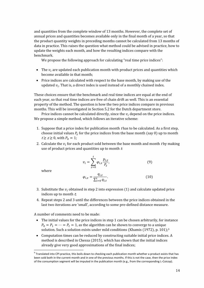
Figure 4 compares the two price indices for men’s socks and T-shirts.10 The results

show large differences for T-shirts. The direct method does not capture the contribution of

new products to price change in the year of introduction into the assortment. New types of

T-shirts, made of organic cotton, were introduced in 2010 at high initial prices, which

started to decrease after a few months. This price decrease is captured by the QU-index.

The direct index only evidences the price behaviour of the existing part of the assortment,

which, in contrast to the new items, mainly shows a price increase in 2010.

The examples show that it is important to have an index method in which not only

existing items enter the calculations, but in which also new items are timely included. This

10

The results for T-shirts differ from the those in Chessa (2015) and Chessa et al. (2015), since a subset of the data was used in the cited papers. However, the findings are the same as in the present study.

16

means that the 𝑣𝑖 should be calculated for new products as soon as these appear in an

assortment.11

Figure 4. Real time QU-indices compared with direct index (5) for men’s socks and T-shirts, based on scanner data of the department store (Feb. 2009 = 100).

5.2 Comparisons with a transitive benchmark index

Price indices for consumption segments are calculated according to the algorithm in

Section 4.3, which computes real time indices. The resulting indices are free of chain drift

by construction, as they are equal to the transitive benchmark indices at the end of each

year. Benchmark indices are calculated each month with yearly fixed product specific

quantity weights 𝑣𝑖, which are based on price and quantity data from 13 months. In the

real time index, the 𝑣𝑖 are updated each month, which raises the question how the real

time and benchmark indices compare throughout a publication year.

Real time and benchmark indices were compared for a large sample from the scanner

data of the Dutch department store, which covers almost 60 per cent of the total 4-year

turnover in the period February 2009-March 2013. Seven Coicops were involved in the

comparison: food and non-alcoholic beverages, menswear, ladies’ wear, children and baby

clothing, household textiles, products for personal care, and restaurants. QU-indices were

calculated for each consumption segment in these Coicops, which were aggregated to

Coicop and overall indices according to Laspeyres type indices, with turnover shares from

the preceding year serving as weights.

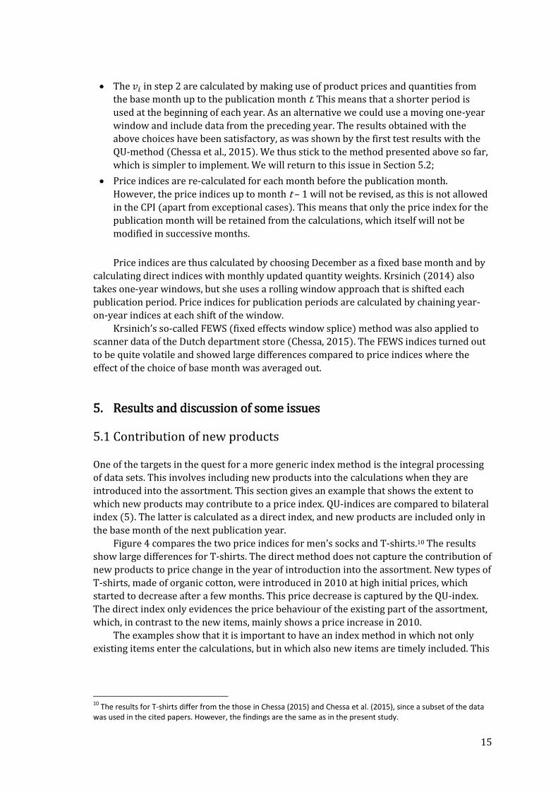
The overall price indices are shown in Figure 5, that is, for the seven (L-)Coicops

combined. The differences throughout the 4-year period are small. The year-on-year

indices differ by one to several tenths of a percentage point. Averaged over the whole 4-

year period, the price indices are equal up to the tenth percentage point.

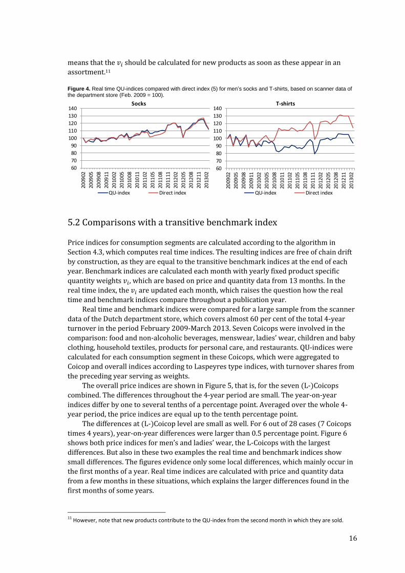
The differences at (L-)Coicop level are small as well. For 6 out of 28 cases (7 Coicops

times 4 years), year-on-year differences were larger than 0.5 percentage point. Figure 6

shows both price indices for men’s and ladies’ wear, the L-Coicops with the largest

differences. But also in these two examples the real time and benchmark indices show

small differences. The figures evidence only some local differences, which mainly occur in

the first months of a year. Real time indices are calculated with price and quantity data

from a few months in these situations, which explains the larger differences found in the

first months of some years.

11

However, note that new products contribute to the QU-index from the second month in which they are sold.

60

70

80

90

100

110

120

130

140

2009

02

2009

05

2009

08

2009

11

2010

02

2010

05

2010

08

2010

11

2011

02

2011

05

2011

08

2011

11

2012

02

2012

05

2012

08

2012

11

2013

02

Socks

QU-index Direct index

60

70

80

90

100

110

120

130

140

2009

02

2009

05

2009

08

2009

11

2010

02

2010

05

2010

08

2010

11

2011

02

2011

05

2011

08

2011

11

2012

02

2012

05

2012

08

2012

11

2013

02

T-shirts

QU-index Direct index

17

Figure 5. Real time and transitive benchmark indices for seven Coicops combined for the Dutch department store (Feb. 2009 = 100).

Figure 6. Real time and transitive benchmark indices for men’s and ladies’ wear for the Dutch department store (Feb. 2009 = 100).

5.3 Comparisons with two variants

As was stated previously in this paper, the Geary-Khamis method has been the subject of

discussion in international price comparisons about a phenomenon known as the

Gerschenkron effect or substitution bias. International reference prices of commodities

(i.e., the 𝑣𝑖, with time replaced by country) tend to the prices of larger countries because of

the quantity based weighting of prices. If the larger countries exhibit higher prices than

the other countries in the comparison, then the resulting reference prices are felt to

contradict with economic theory, as consumers tend to buy more of some good when

prices decrease.

The question is to what extent this substitution bias would affect the results in

intertemporal comparisons. Chessa (2015) already investigated non-linear forms for the

𝑣𝑖. The resulting price indices hardly differ from the base QU-method. The first results in

comparing the base method with variants that should suffer less in theory from the

substitution bias were thus encouraging.

The present paper considers yet two other variants of the method. The only difference

with the base method lies again in the definition of the 𝑣𝑖, this time in the weighting

applied to the deflated prices in expression (7):

60

70

80

90

100

110

120

130

140

2009

02

2009

05

2009

08

2009

11

2010

02

2010

05

2010

08

2010

11

2011

02

2011

05

2011

08

2011

11

2012

02

2012

05

2012

08

2012

11

2013

02

Real time index Benchmark index

60

70

80

90

100

110

120

130

140

2009

02

2009

05

2009

08

2009

11

2010

02

2010

05

2010

08

2010

11

2011

02

2011

05

2011

08

2011

11

2012

02

2012

05

2012

08

2012

11

2013

02

Menswear

Real time index Benchmark index

60

70

80

90

100

110

120

130

140

2009

02

2009

05

2009

08

2009

11

2010

02

2010

05

2010

08

2010

11

2011

02

2011

05

2011

08

2011

11

2012

02

2012

05

2012

08

2012

11

2013

02

Ladies' wear

Real time index Benchmark index

18

In the first variant, the deflated prices are weighted according to a month’s share in

the sum of expenditure shares of a product over different months;

In the second variant, each month receives equal weight.

The first variant leads to a method that was called the “equally weighted GK-method”

(Hill, 2000). In this study we simply refer to this method as a variant with turnover share based weights. If we denote the expenditure share of product 𝑖 in period t by 𝑤𝑖,𝑡, then the

weights of the deflated prices in the 𝑣𝑖 become

𝜑𝑖,𝑧 =𝑤𝑖,𝑧

∑ 𝑤𝑖,𝑠𝑡𝑠=0

, (11)

where t ≥ z ≥ 0 denotes the publication month. Expression (11) is used in the calculation

of real time indices, which replaces expression (10) in the algorithm of Section 4.3.12

The second variant applies the following weighting in the 𝑣𝑖:

𝜑𝑖,𝑧 =𝛿𝑖,𝑧

∑ 𝛿𝑖,𝑠𝑡𝑠=0

, (12)

where 𝛿𝑖,𝑡 = 1 if 𝑞𝑖,𝑡 > 0, and 𝛿𝑖,𝑡 = 0 otherwise. In other words, deflated prices in months

with sales receive the same weight. This method is referred to as the equally weighted

variant of the base method.

At first sight, it might seem odd to ignore the actual sales figures in the product

quantity weights and only include the information whether a product has been sold or not

in a month. However, a deeper analysis shows that weighting scheme (12) leads to an

interesting variant of the base QU-method: under certain conditions, the price index in the

bilateral case is equal to the Fisher index.13 For this observation alone it is interesting to

include the second variant in the comparison. But also because weighting scheme (12)

may lead to completely different weights compared to (10). The question then is to what

extent the differences between schemes (10) and (12) affect the price indices.

Real time price indices were computed for both variants according to the algorithm of

Section 4.3, which are compared below with the base method. The same data as in Section

5.2 were used for this purpose. It must be stressed that a threshold was applied in the

equal weighting variant. This was done in order to prevent out-of-season prices and dump

prices of outgoing GTINs to receive disproportionally large weights compared with the

usually very low sales. However, a very mild threshold was set: prices were excluded from

the index calculations if quantities sold decrease more than 90 per cent with respect to

“regular sales” (quantities sold averaged over past months in which the threshold is

satisfied).

Figure 7 shows the real time indices for the base method and the two variants for the

Dutch department store, for the seven (L-)Coicops combined. The three price indices can

12

It should be noted that summing turnover or expenditure shares over different time periods is not allowed from the viewpoint of the theory of measurement scales. Shares in different periods represent measurements from ratio scales with different scaling factors. The first variant is included in the comparison because it has been suggested as an alternative to the GK-method in PPP-studies. Expenditure share based weighting is also used in other multilateral price index methods, like the time product dummy index. 13

This holds in the situation where the turnover share of matched products is the same in both periods, and in the case where the prices of all unmatched items are imputed. The general expression of the index formula is more complex. Details are left out in this study.

19

hardly be distinguished. The variant with equal weights lies remarkably close to the price

index for the base method. The year-on-year indices for the base method are 0.25

percentage point higher on average. The differences between the base method and the

variant with turnover share based weights are 0.1 percentage point smaller on average.

Figure 7. Overall price index for the Dutch department store according to the base method, compared with the price indices for the two variants of the method (Feb. 2009 = 100).

The differences for the underlying seven Coicops are small as well. The largest

differences are found for clothing. Figure 8 shows the three price indices for menswear

and ladies’ wear. The differences between the year-on-year indices lie within 0.5

percentage point in most years.

Figure 8. Price indices for men’s and ladies’ wear for the Dutch department store, for the base method and the two variants (Feb. 2009 = 100).

Although the comparative study in this section is empirical, it is important to

emphasise the small differences found between the base method and the two variants. The

results show that the substitution effect, if present at all, is very small, not only at overall

level, but also for the underlying (L-)Coicops. The differences at consumption segment

level are somewhat larger, but are consistently small at this most detailed level as well.

It is important to continue these comparative analyses for other retailers and

consumer goods, also with regard to the analyses in Section 5.2. This has been done within

the scope of this research also for mobile phones and for a small subset of items sold by

do-it-yourself stores. The conclusions are the same as reported above. This means that the

results for the base method look very robust, showing small variations under different

choices in the weighting of the deflated prices.

60

70

80

90

100

110

120

130

140

2009

02

2009

05

2009

08

2009

11

2010

02

2010

05

2010

08

2010

11

2011

02

2011

05

2011

08

2011

11

2012

02

2012

05

2012

08

2012

11

2013

02

Base method Turnover share based Equal weights

60

70

80

90

100

110

120

130

140

2009

02

2009

05

2009

08

2009

11

2010

02

2010

05

2010

08

2010

11

2011

02

2011

05

2011

08

2011

11

2012

02

2012

05

2012

08

2012

11

2013

02

Menswear

Base method Turnover share based Equal weights

60

70

80

90

100

110

120

130

140

2009

02

2009

05

2009

08

2009

11

2010

02

2010

05

2010

08

2010

11

2011

02

2011

05

2011

08

2011

11

2012

02

2012

05

2012

08

2012

11

2013

02

Ladies' wear

Base method Turnover share based Equal weights

20

6. First CPI production experiences

The methodology has been implemented last year after one year of methodological

research. It has been tested on scanner data of the department store and on electronic

transaction data of mobile phones. A summary of different research and pre-testing

phases for the department store data, from text mining and attribute selection to index

calculation and validation of the results, is described in Chessa et al. (2015). The

implementation for the department store is in a final testing phase. Different scenarios are

being run in order to make final decisions on product homogeneity for some item groups.

The methodology is part of the CPI for mobile phones since January 2016. This section

gives a summary of different process stages, from data analysis and attribute selection

until production.

Data analysis

The data cover the period December 2013 until December 2015. For every device, the data

include transaction prices, numbers of devices sold and information on item attributes,

either as a separate record variable or contained in the item description. Record variables

were reported for each device in every month. Outliers were not detected among prices of

devices. A number of potentially relevant item attributes are not included in the data,

amongst which all processor characteristics (e.g., speed, number of cores), working

memory and screen resolution.

Attribute selection and homogeneous products

Additional attributes were collected from a web site for a smaller set of 70 devices, which

together cover about 75% of the 2-year turnover. A set of 12 attributes was analysed by

applying a sensitivity analysis as described in Section 3. The first step in this analysis was

to quantify the impact of each attribute separately on the unit value index. Next, the most

influential attribute was selected and others were added in order to quantify their

additional contribution to the year-on-year index. Five attributes completely determine

the index. Most attributes seem to be correlated, in the sense that, for instance, devices

with a higher screen resolution tend to have a more powerful processor.

From the set of 5 attributes, Near Field Communication was left out since paying by

smartphone is still in a pilot phase in The Netherlands. This may change in the coming

years, in which case NFC could be added as a relevant attribute. Long Term Evolution

(LTE/4G) adds less than 0.01 percentage point to the year-on-year price index, so that LTE

was omitted as well. Moreover, the majority of the smartphones is currently equipped

with LTE. This share is still growing, so we do not expect this attribute to contribute much

to product differentiation.

Three attributes were thus eventually selected: brand, internal storage capacity and

“performance”. The latter is measured by a benchmark test score (Geekbench), which

indicates how different components of a device act together when performing CPU and

GPU tasks (processor type/model, number of cores, working memory). Benchmark scores

are obviously not included in the data, so we collect scores from the internet. This has

been done now for more than 130 devices, which cover 88 per cent of the total 2-year

turnover. Benchmark scores are subdivided into three segments (high, medium and lower

performing devices). Refinements to 4 or 5 segments did not affect the price index

significantly.

21

Price index

Index calculations were run based on the aforementioned choices on the three selected

attributes. The implementation of homogeneous products and the index method was

controlled and found to be correct after a series of test runs. An important part of these

checks is the derived series. VAT is the only tax measure of interest for mobile phones. The

QU-method handles VAT changes correctly (and also excise measures).

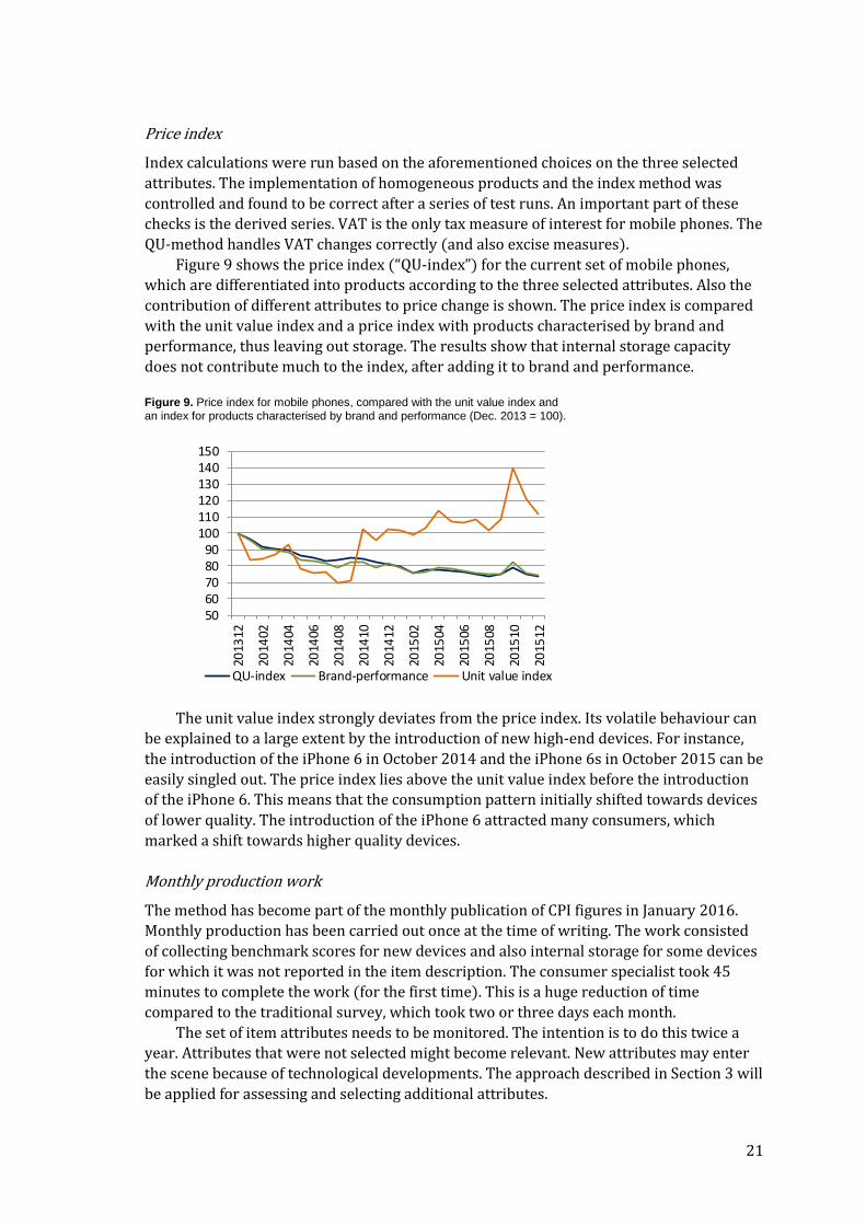
Figure 9 shows the price index (“QU-index”) for the current set of mobile phones,

which are differentiated into products according to the three selected attributes. Also the

contribution of different attributes to price change is shown. The price index is compared

with the unit value index and a price index with products characterised by brand and

performance, thus leaving out storage. The results show that internal storage capacity

does not contribute much to the index, after adding it to brand and performance.

Figure 9. Price index for mobile phones, compared with the unit value index and an index for products characterised by brand and performance (Dec. 2013 = 100).

The unit value index strongly deviates from the price index. Its volatile behaviour can

be explained to a large extent by the introduction of new high-end devices. For instance,

the introduction of the iPhone 6 in October 2014 and the iPhone 6s in October 2015 can be

easily singled out. The price index lies above the unit value index before the introduction

of the iPhone 6. This means that the consumption pattern initially shifted towards devices

of lower quality. The introduction of the iPhone 6 attracted many consumers, which

marked a shift towards higher quality devices.

Monthly production work

The method has become part of the monthly publication of CPI figures in January 2016.

Monthly production has been carried out once at the time of writing. The work consisted

of collecting benchmark scores for new devices and also internal storage for some devices

for which it was not reported in the item description. The consumer specialist took 45

minutes to complete the work (for the first time). This is a huge reduction of time

compared to the traditional survey, which took two or three days each month.

The set of item attributes needs to be monitored. The intention is to do this twice a

year. Attributes that were not selected might become relevant. New attributes may enter

the scene because of technological developments. The approach described in Section 3 will

be applied for assessing and selecting additional attributes.

5060708090

100110120130140150

2013

12

2014

02

2014

04

2014

06

2014

08

2014

10

2014

12

2015

02

2015

04

2015

06

2015

08

2015

10

2015

12

QU-index Brand-performance Unit value index

22

7. Final remarks

The differences across index methods that make use of electronic data sets in the Dutch

CPI, in conjunction with the increased use of such data, motivated a search towards a more

generic index method. To this end, a methodology for characterising homogeneous

products and for calculating price indices has been developed. The question whether the

methodology can be applied to data sets of different retailers and consumer goods can be

answered in a positive way.

The methodology that encompasses product differentiation and price index

calculation (sections 3 and 4) allows integral data processing, without applying turnover

or dump price filters, irrespective of retailer and type of consumer good. The methodology

has been applied to a broad range of consumer goods, which include the broad assortment

of a department store, mobile phones, items sold by do-it-yourself (DIY) stores and

drugstores.

The methodology has recently been incorporated into monthly CPI production for

mobile phones. First experiences have shown that the methodology works efficiently and

hardly requires manual work, which was reduced from two or three days for the

traditional survey to 45 minutes with the current methodology. The amount of time

needed is expected to decrease when more experience is gained with the methodology.

CPI production for the department store scanner data is expected to be realised

within several months. Meanwhile, the application of the methodology to other scanner

data sets is being investigated, in particular for DIY-stores. A test data set with information

about additional attributes for paint and electrical equipment has been analysed, which

also includes SKUs for each item. The SKUs enable us to link outgoing GTINs to follow-up

items, which makes it possible to capture possible price increases under relaunches. First

analyses on the possible use of SKUs look promising. In addition, SKUs hardly require

monthly production work since item attributes are not needed to link old and new GTINs.

The QU-method makes it possible to include new items into the index calculations as

soon as items are introduced into an assortment. This is a desirable property, since

postponing the inclusion of new items until the next base month may have a big impact on

a price index (Section 5.1). The product quantity weights are exclusively based on

consumption patterns from the current year of publication. This is a major difference and

contribution compared to traditional methods.

The product quantity weights are updated every month, so that the weights are time

dependent. However, price indices for publication months are free of chain drift by

construction. The differences with transitive benchmark indices appear to be very small

throughout the year, which vanish at the end of each year. There may be some room for

improving price index calculations for the first months of a year, as information from a few

months is used for calculating the quantity weights. This could be a topic for further

research. But given the small differences between the real time and benchmark indices

reported in Section 5.2, this does not seem to be a big issue.

The empirical study of Section 5.3 suggests that the possible impact of the

substitution bias is very small or can even be ignored. One of the two variants of the base

QU-method turned out to be very interesting, which is the one with equal weights applied

to the deflated prices. The price indices for this variant show (very) small differences with

the price indices for the base method. This is an intriguing result, which deserves further

study, not only empirically, but also from a theoretical perspective.

23

To these remarks it seems worth adding two observations. First, the comparable

results obtained for the equal weights variant may reveal to be a very useful finding in

view of the rapidly increasing popularity of using internet prices collected from web

scraping in price index methods. The motivation to investigate this variant further

obviously lies in the weights of the deflated prices in expression (12), which does not

require exact figures on quantities sold, only whether an item is sold. On the other hand, it

can be realistically expected that some form of weighting across products will be needed.

At what level of detail, and what secondary sources could be used for this purpose, is a

question of future research.

A second observation could be made with regard to international price comparisons:

Could the equal weights variant be an interesting alternative to explore, given the past

debates on the substitution effect for the GK-method?

The mentioned topics for further research could be considered within the context of a

4-year research programme at Statistics Netherlands, which started in 2015. One of the

aims of the programme is to extend comparative studies to a broader range of index

methods (de Haan et al., 2016).

References

Balk, B.M. (1996). A comparison of ten methods for multilateral international price and

volume comparison. Journal of Official Statistics, 12: 199-222.

Balk, B.M. (2001). Aggregation methods in international comparisons: What have we

learned? Paper originally prepared for the Joint World Bank - OECD Seminar on

Purchasing Power Parities, 30 January - 2 February 2001, Washington DC.

Balk, B.M. (2012). Price and Quantity Index Numbers: Models for Measuring Aggregate Change and Difference. Cambridge, UK: Cambridge University Press.

Chessa, A.G. (2013). Comparing scanner data and survey data for measuring price change

of drugstore articles. Paper presented at the Workshop on Scanner Data for HICP, 26-27

September 2013, Lisbon, Portugal.

Chessa, A.G. (2015). Towards a generic price index method for scanner data in the Dutch

CPI. Ottawa Group Meeting, 20-22 May 2015, Urayasu City, Japan.

Chessa, A.G., Boumans, S., and Walschots, J. (2015). Towards a new methodology for

processing scanner data in the Dutch CPI. Paper presented at the Workshop on Scanner Data, 1-2 October 2015, Rome, Italy.

Claeskens, G., and Hjort, N.L. (2008). Model Selection and Model Averaging. Cambridge

University Press, UK.

Diewert, W.E. (2011). Methods of aggregation above the basic heading level within

regions. In Measuring the Size of the World Economy. ICP Book, Chapter 5.

24

Geary, R. C. (1958). A note on the comparison of exchange rates and purchasing power

between countries. Journal of the Royal Statistical Society A, 121: 97-99.

van der Grient, H.A., and de Haan (2010). The use of supermarket scanner data in the

Dutch CPI. Paper presented at the Joint ECE/ILO Workshop on Scanner Data, 10 May 2010,

Geneva.

de Haan, J. (2006). The re-design of the Dutch CPI. Statistical Journal of the United Nations Economic Commission for Europe, 23: 101-118.

de Haan, J. and van der Grient, H.A. (2011). Eliminating chain drift in price indexes based

on scanner data. Journal of Econometrics, 161: 36-46.

Haan, J. de, Willenborg, L., and Chessa, A.G. (2016). An overview of price index methods for

scanner data. Internal report, Statistics Netherlands.

Hill, R.J. (2000). Measuring substitution bias in international comparisons based on

additive purchasing power parity methods. European Economic Review, 44, 145-162.

Khamis, S. H. (1972). A new system of index numbers for national and international

purposes. Journal of the Royal Statistical Society A, 135: 96-121.

Krsinich, F. (2014). The FEWS Index: Fixed Effects with a Window Splice – Non-revisable

quality-adjusted price indexes with no characteristic information. Paper presented at the

Meeting of the Group of Experts on Consumer Price Indices, 26-28 May 2014, Geneva,

Switzerland.

Walschots, J. (2016). Fifteen years of new data collection: Looking back and forward.

Paper to be presented at the Meeting of the Group of Experts on Consumer Price Indices,

2-4 May 2016, Geneva, Switzerland.