Process optimization for zero-liquid discharge

desalination of shale gas flowback water under

uncertainty

Viviani C. Onishi a, *, Rubén Ruiz-Femenia a, Raquel Salcedo-Díaz a, Alba Carrero-

Parreño a, Juan A. Reyes-Labarta a, Eric S. Fraga b, José A. Caballero a

a Institute of Chemical Process Engineering, University of Alicante, Ap. Correos 99,

Alicante 03080, Spain

b Centre for Process Systems Engineering, Department of Chemical Engineering,

University College London, London WC1E 7JE, UK

* Corresponding author at. Institute of Chemical Process Engineering, University of

Alicante, Ap. Correos 99, Alicante 03080, Spain. Phone: +34 965903400. E-mail

addresses: viviani.onishi@ua.es / viviani.onishi@pq.cnpq.br (Viviani C. Onishi).

2

ABSTRACT

Sustainable and efficient desalination is required to treat the large amounts of high-

salinity flowback water from shale gas extraction. Nevertheless, uncertainty associated

with well data (including water flowrates and salinities) strongly hampers the process

design task. In this work, we introduce a new optimization model for the synthesis of

zero-liquid discharge (ZLD) desalination systems under uncertainty. The desalination

system is based on multiple-effect evaporation with mechanical vapor recompression

(MEE-MVR). Our main objective is energy efficiency intensification through brine

discharge reduction, while accounting for distinct water feeding scenarios. For this

purpose, we consider the outflow brine salinity near to salt saturation condition as a design

constraint to achieve ZLD operation. In this innovative approach, uncertain parameters

are mathematically modelled as a set of correlated scenarios with known probability of

occurrence. The scenarios set is described by a multivariate normal distribution generated

via a sampling technique with symmetric correlation matrix. The stochastic multiscenario

non-linear programming (NLP) model is implemented in GAMS, and optimized by the

minimization of the expected total annualized cost. An illustrative case study is carried

out to evaluate the capabilities of the proposed new approach. Cumulative probability

curves are constructed to assess the financial risk related to uncertain space for different

standard deviations of expected mean values. Sensitivity analysis is performed to appraise

optimal system performance for distinct brine salinity conditions. This methodology

represents a useful tool to support decision-makers towards the selection of more robust

and reliable ZLD desalination systems for the treatment of shale gas flowback water.

Keywords: Shale gas flowback water; Multiple-effect evaporation with mechanical

vapor recompression (MEE-MVR); Zero-liquid discharge (ZLD); Uncertainty; Risk

management; Robust design.

3

1. Introduction

Shale gas production is a promising energy source to address the increasing global

demand. Advances in horizontal drilling and hydraulic fracturing (“fracking”)

technologies allied to economic factors that include supply reliability, have driven growth

in unconventional natural gas production from shale reserves (Cooper et al., 2016; Xiong

et al., 2016). In the United States (U.S.), recent projections of the Energy Information

Administration indicate that shale gas can reach 30% of all natural gas produced in the

world by 2040 (EIA, 2016a, 2016b). Notwithstanding, one of the biggest challenges for

promoting further development and cleaner production of shale gas relies on optimal

management of flowback water (Vidic et al., 2013). This is mainly due to the large

amounts of high-salinity wastewater generated during shale gas extraction (Huang et al.,

2016).

Drilling and fracking of horizontal wells requires elevated quantities of water-

based fracturing fluid to create a fractures network, and release gas trapped into tight shale

formations (Chen and Carter, 2016). Depending on the shale rocks characteristics, gas

exploration of one single well demands between 10 500–21 500 m3 (~3–6 million gallons)

of water (Ghanbari and Dehghanpour, 2016; Jacquet, 2014). However, other authors

suggest this amount can be even higher, reaching 30 000 m3 (~8 million gallons) per well

completion (Hammond and O’Grady, 2017). The injection fluid is predominantly

constituted by proppant (sand and water mixture, ∼98%) and chemical enhancers

(corrosion inhibitors, friction reducers, surfactants, flow improvers, etc.) (Stephenson et

al., 2011). Several reports indicate a range of 10–80% of the total amount of fracking

fluid that returns to ground as flowback water, during the first two weeks from well

operations start (Hammond and O’Grady, 2017; Slutz et al., 2012). Table 1 presents shale

4

gas flowback water information and average water amounts needed for horizontal drilling

and hydraulic fracturing processes in prominent U.S. shale plays.

For lessening environmental damage, shale gas flowback water should be

reclaimed to be recycled or reused as injection fluid for new wells exploitation. In any

case, shale gas wastewater demands specific pre-treatment—that comprises filtration,

physical and chemical precipitation, flotation and sedimentation—and effective

desalination to allow its reuse or safe disposal (Carrero-Parreño et al., 2017). In addition

to chemical additives and other pollutants (e.g., organic matter, particulates, greases, and

radioactive elements, to name a few) (Vengosh et al., 2013), hypersaline concentrations

in shale gas flowback water can be hazardous to human health and the environment

(Vengosh et al., 2014). Desalination technologies should play a key role in hydrological

planning schemes for optimal water resources management in shale gas production.

Due to aforementioned reasons, advanced and more efficient technologies for

flowback water desalination should be developed for enhancing general sustainability and

efficiency in shale gas industry (Onishi et al., 2017a; 2017b). Nevertheless, great

uncertainty associated with well data (including flowback water flowrates and salinities)

strongly hampers the optimal process design. Generally, a deterministic approach (i.e.,

system design and optimization considering a single set of process inlet conditions)

cannot provide all required system flexibility under process parameters variability. This

methodology could lead to weak system performance represented by sub-optimal

solutions, when considering different feeding scenarios. In addition, this approach does

not provide any information to the decision maker on the impact of uncertain parameters

on the design chosen.

Design and optimization under uncertainty have received increased interest by the

literature in last years (see Sahinidis (2004) for general information about the subject).

5

Some authors have directed their efforts to optimize water management in shale gas

process under uncertainty. For instance, Yang et al. (2014) have presented an stochastic

model for optimizing shale gas fracturing schedule, in accordance to water transportation,

and wastewater treatment and reuse, by considering uncertain water availability. In Zhang

et al. (2016), a mathematical model has been proposed to determine the optimal flowback

water treatment and disposal options for water management during shale gas operations.

In their work, the data uncertainty is modelled via a hybrid fuzzy-stochastic approach.

Additional notable contributions are addressed by Gao and You (2015) and Lira-Barragán

et al. (2016). In spite of these attempts to optimize water management, research about

shale gas flowback water desalination under uncertainty is still in its first steps.

Different desalination processes can be applied for desalination of high-salinity

wastewater, which encompasses membrane and thermal-based technologies. The first

group includes reverse osmosis (RO) and multistage membrane distillation (MD), while

the second one comprises multistage flash distillation (MSF) and single/multiple-effect

evaporation systems with/without mechanical or thermal vapor recompression

(SEE/MEE-MVR/TVR). In a recent study, Boo et al. (2016) have experimentally

evaluated the performance of direct contact MD for the shale gas wastewater desalination,

by using a modified omniphobic membrane. Also, Jang et al. (2017) have evaluated the

suitability of three different desalination techniques for salt removal from shale gas

wastewater: MD, RO and evaporative crystallization (EC). Their results show relatively

higher efficiencies for MD and EC in comparison with the RO process. According to

Shaffer et al. (2013), multiple-effect evaporation with mechanical vapor recompression

(MEE-MVR) processes are frequently more advantageous than membrane-based

processes for shale gas wastewater applications. As a consequence of lower susceptibility

6

to fouling and rusting problems, MEE-MVR systems often require less intensive pre-

treatment processes.

Michel et al. (2016) have performed an experimental study on pre-treatment and

desalination of shale gas flowback water. The authors have considered a two-stage

treatment process composed by pre-treatment technologies (filtration, pH adjustment,

oxidation and sedimentation) and posterior nanofiltration/RO desalination. Results

obtained in their work emphasize the need for very effective pre-treatment before

membrane desalination becomes possible. Cho et al. (2016) have studied the application

of anti-scalants to diminish scale formation in MD desalination of flowback water from

shale gas fracking. Note that other benefits of MEE desalination systems are related to

facility of scaling and dealing with non-condensable gases (Shen et al., 2015), in addition

to a lower operation temperature that reduces equipment sizing and insulation (El-

Dessouky and Ettouney, 1999). Although previous studies represent important

improvements for shale gas wastewater treatment, none of them has contemplated zero-

liquid discharge (ZLD) operation.

A ZLD process has been investigated by Thu et al. (2015), through multiple-effect

adsorption applied to seawater desalination. Tong and Elimelech (2016) have critically

reviewed the driving forces, technologies and environmental impacts of ZLD as an

prominent strategy for wastewater management. In their work, the authors have examined

the advantages and limitations of both membrane and thermal-based ZLD technologies.

Chung et al. (2016) have proposed multistage vacuum membrane distillation for ZLD

desalination of high-salinity water. The latter authors have used a finite differences-based

method for the numerical simulation of the process, by allowing salt concentration in

brine discharges near to saturation condition. On the other hand, Han et al. (2017) have

developed mathematical models for SEE and MEE-MVR processes simulations of ZLD

7

seawater desalination. Through energy and exergy analyses, the authors have concluded

that MEE are often more attractive than single-effect systems, due to lower compressor

power consumption. However, their study lacks a comprehensive cost analysis.

For addressing the application of ZLD to shale gas flowback water desalination,

Onishi et al. (2017b) have developed a mathematical model for optimal design of

SEE/MEE systems with single or multistage MVR and heat integration. The non-linear

programming (NLP) model has been based on a general superstructure, including feed

pre-heating, multiple evaporation effects with flash separation and multistage

intercooling compression. Still, the authors have performed a thorough comparison

between the optimal SEE/MEE (with/without multistage compression) systems

configurations obtained, in terms of their capability to produce freshwater and achieve

ZLD conditions under different wastewater inlet salinities. Energy and economic analyses

indicate the MEE process with single-stage compression as the most cost-effective

process for desalting shale gas flowback water. With this important result in mind, Onishi

et al. (2017a) have proposed a new rigorous optimization approach by the consideration

of a more accurate calculation of heat transfer coefficients. Moreover, the authors have

included the modelling of major equipment features, which allows the estimation of the

optimal number and length of tubes, and the shell diameter of the evaporator. Then,

uncertainty related to data from shale gas can be considered during the design task of the

above-mentioned processes for improving system flexibility and robustness.

Into this framework, we introduce a new mathematical model for optimal design

of ZLD evaporation systems under correlated data uncertainty. The multistage

superstructure is defined by multiple-effect evaporation process with heat integration and

mechanical vapor recompression (MEE-MVR). The MEE-MVR process is based on our

previous study (Onishi et al., 2017b), in which the system is composed of several

8

evaporation effects with horizontal falling film tubes coupled to flashing tanks and an

electric-driven compressor. Our main goal is energy efficiency intensification of shale

gas flowback water desalination through lessening brine discharges, while accounting for

distinct water feeding scenarios. For this purpose, ZLD process is ensured by a design

constraint that defines the outflow brine salinity near to the salt saturation condition—

note that, under the latter restriction, the proposed MEE-MVR system will technically

achieve brine discharges close to ZLD conditions. Brine crystallizer or evaporation ponds

are still required to remove remaining water amounts from the brine to reach the real ZLD

condition—. To the best of our knowledge, this is the first study assessing the impacts of

data uncertainty on the optimal design of ZLD evaporation systems, specially developed

for shale gas flowback water desalination. Furthermore, we emphasize that important

improvements on the process are implemented, including the use of an external energy

source to avoid oversized equipment.

In this new approach, feed water salinity and flowrate are both considered as

uncertain design parameters. These uncertain parameters are mathematically modelled as

a set of correlated scenarios with given probability of occurrence. Scenarios generated by

MATLAB are described by multivariate normal distribution, via sampling technique

based on symmetric correlation matrix. The stochastic multiscenario NLP-based model

is optimized in GAMS, through the minimization of the expected total annualized cost.

An illustrative case study is performed to evaluate the capabilities of the proposed new

modelling stochastic methodology. Cumulative probability curves are constructed for the

assessment of financial risk associated with the uncertain parameters space for different

standard deviations of mean values. Additionally, sensitivity analysis is carried out to

appraise optimal system performance for distinct brine salinity conditions.

9

This paper is organized as follows: In Section 2, we properly define the problem

of interest. Section 3 presents the detailed description of the MEE-MVR superstructure

proposed for the desalination of shale gas flowback water. The stochastic multiscenario

NLP model is developed in Section 4, while the scenario generation is explained in

Section 5. The impact of uncertainty on MEE-MVR system design is assessed in Section

6, using a shale gas case study based on uncertain real data. Finally, we summarize the

main conclusions in the last section.

2. Problem statement

The problem of interest is formally stated as follows. Given is a stream of high-salinity

shale gas flowback water, which requires effective desalination treatment. The shale gas

flowback water stream has known inlet conditions (defined by its temperature, pressure

and uncertain salinity and flowrate) and a target state described by the ZLD brine

discharge specification (i.e., 300 g kg-1). In addition, a MEE-MVR desalination system

(composed by multiple-effect evaporator, flashing tanks, preheater, mechanical

compressor, mixers and pumps) and energy services (electricity and steam) are also

provided with their corresponding costs. The main objective is to achieve energy

efficiency intensification of flowback water desalination process by lessening brine

releases, while accounting for distinct water feeding scenarios. Furthermore, we consider

that both salinity and flowrate of shale gas flowback water are uncertain design

parameters that can be expressed through different correlated scenarios (each one

presenting different water feeding conditions). Note that the data uncertainty is associated

with the great variability presented in data of salt concentrations and flowrates of

wastewater from shale plays. The general superstructure proposed for the optimization of

MEE-MVR desalination process is displayed in Fig. 1.

10

Shale gas flowback water desalination can be performed after specific pre-

treatment to remove suspended solids, oils, greases and chemical additives. Further

information about efficient pre-treatment processes applied to shale gas flowback water

is presented in Carrero-Parreño et al. (2017). In this case, we assume that shale gas

flowback water remains with elevated concentration of salts after its pre-treatment. Thus,

the optimal MEE-MVR system design should correspond to the most cost-effective

desalination process, exhibiting reduced brine releases and high freshwater production in

all scenarios. We highlight that energy intensification allied to ZLD operation allows the

reduction of environmental impacts related to energy consumption and wastewater

disposal. For achieving the goals of ZLD process and high freshwater production, we

intend to optimize the MEE-MVR system performance under uncertainty, through the

minimization of the expected total annualized cost. The objective function accounts for

the contributions related to capital investment in equipment (scenario independent

variable), and operational expenses regarding electricity and vapor consumption

(scenario-dependent variables). Moreover, the optimal ZLD operation in the uncertain

search space is ensured by including a design constraint that defines brine discharge

salinity near to salt saturation conditions in each scenario.

The MEE-MVR system optimization for ZLD desalination of shale gas

wastewater under uncertainty is a very difficult task, aimed at obtaining the optimal

system configuration and operational conditions for distinct feeding scenarios. Hence, the

optimal MEE-MVR system should have lower equipment size (represented by heat

transfer areas and compressor capacity) and minimum thermal services (electric power

and steam) consumption. Nonetheless, at the same time, the MEE-MVR system should

be able to efficiently operate in a large range of correlated scenarios. For this purpose, the

decision variables are divided into two sets: the scenario independent and scenario-

11

dependent variables. The first set is not influenced by uncertain parameters, while the

second one is sensitive to the uncertainty in the search space. Sahinidis (2004) have

pointed out scenario-dependent variables as a recourse against any infeasibility that

would arise from a particular materialization of the uncertainty. Typically, equipment

sizes are scenario independent optimization variables. On the other hand, all streams

properties and operating conditions—which include specific enthalpy, specific heat,

temperature, pressure, salinity and flowrate—are unknown scenario-dependent variables

requiring optimization. Fig. 2 displays the main decision variables for the optimization

of: (a) single-stage compressor; and, (b) effect i of the evaporator coupled to flashing tank

i in the MEE-MVR system.

The MEE-MVR system should be operated at low pressures and temperatures to

avoid instability and prevent fouling and rusting problems. For this reason, upper and

lower bounds on temperature and pressures for all feeding scenarios are essential to solve

the problem. Besides the increased number of optimization variables and constraints to

guarantee proper system functioning, the high non-convexity and nonlinearity of some

modelling equations and cost correlations add further complexity to the model. It should

be observed that physical properties, as well as boiling point elevation (BPE), are

functions of streams temperature and salinity that should also be estimated in all scenarios

as shown in Appendix A.

3. Superstructure and process description

The MEE-MVR superstructure proposed for the shale gas flowback water desalination is

essentially composed of the following equipment:

12

(i) Horizontal falling film evaporator with multiple effects.

(ii) Flashing tank separators.

(iii) Single-stage mechanical vapor compressor.

(iv) Shell-and-tube heat exchanger.

(v) Mixers and pumps.

As illustrated in Fig. 1, the MEE-MVR desalination system presents several

evaporation effects coupled to a mechanical vapor compressor and intermediate flashing

tank separators. It is worth to mention that each evaporation effect is composed of a tube-

bundle containing numerous horizontal falling film tubes, demister for droplets separation

and spray nozzles. These equipment pieces are housed inside the shell that should also

have space for saturated vapor and brine concentrate pool. The vapor condensation occurs

inside the horizontal-tubes, while feeding is sprayed onto the tube-bundle to produce a

thin film for water evaporation. Thus, the vapor condensation starts by absorbing latent

heat from the falling film outside tubes. In an opposite way, vaporization occurs due to

the latent heat transferred from condensed vapor in the tube-side. In the first evaporation

effect, the condensate temperature is changed by transferring its sensible heat. As a result,

this variable is decreased from its inlet superheated condition to the outlet temperature

corresponding to vapor saturation pressure.

Vaporization and condensation processes are strongly affected by a variety of

factors, including fluid velocities (Reynolds number), vaporization temperature (changed

by the BPE), streams' physical properties, and geometrical equipment features (e.g., tube

pattern arrangement, and external and internal tube diameters) (Abraham and Mani,

2015). Additional information about the effects of these parameters on the optimal MEE-

MVR system configuration and operational conditions are presented in Onishi et al.

13

(2017a). Since horizontal-tube falling film arrangements presents higher heat transfer

coefficients than vertical ones, these type of configuration exhibits reduced equipment

size and, therefore, lower capital investment (Qiu et al., 2015).

Flashing tanks are placed between evaporation effects to recover energy from

condensate vapor (or distillate) by reducing its pressure (and temperature). Hence, this

type of equipment allows improving the system energy performance through heat

integration. As the flashed off condensate vapor in an i-effect is added together with the

vapor from the boiling process to the next effect, both streams should present the same

pressure. In spite of pressure equality, these streams can be at different temperatures. So,

mixers should be included in the superstructure. As aforementioned, energy and

economic analyses performed in our previous work (Onishi et al., 2017b) have revealed

that MEE systems with single-stage compression are generally more cost-effective

(freshwater production cost of 6.70 US$ per cubic meter with 2.78 US$ of electric power

consumed per freshwater cubic meter) than multistage compression ones for the ZLD

desalination of shale gas flowback water. This result is mainly due to the capital cost

related to the equipment acquisition and the cooling expenses required by intercooling

multistage compressors. For this reason, a single-stage mechanical vapor compressor

driven by electricity is used to operate on closed vapor recompression cycle.

Consequently, all vapor generated in the system (by feed evaporation and flash

separation) is superheated via compression to meet evaporation energy requirements.

Due to the electric-driven compressor, the MEE-MVR system does not need other

energy sources. However, we consider steam as an additional energy supply for the

desalination system to avoid oversized equipment. As above-mentioned, equipment

capacities are scenario independent decision variables. Therefore, process optimization

for obtaining a system able to operate in a large range of feeding scenarios can lead to

14

worst case sizing solutions. In other words, the equipment should be large enough to deal

with extreme feeding conditions. As there is an optimal trade-off between the equipment

size (capital cost) and energy consumption (operational expenses), it is clearly possible

to reduce the equipment capacity by providing an external energy source. Finally, the

MEE-MVR system also contains a shell-and-tube heat exchanger used to preheat the

shale gas flowback water (henceforth referred as feed water), by taking advantage of

sensible energy from condensed vapor. Obviously, this equipment promotes further heat

transfer enhancement of the ZLD system. Moreover, feed preheating is essential to

maintain the process productivity throughout annual climate changes.

A backward feeding configuration is admitted, so that preheated water is

introduced in the last evaporator effect i, whereas brine (from previous effects) is added

as feed water to the effects 1 to (i-1). As a consequence of the backward configuration,

brine should flow from the last effect towards the first one. However, vapor generated in

the effects and flashed off vapor is conducted towards the last evaporation effect, where

it is sent to the compressor to be used as energy source to drive the ZLD system. Because

vapor streams follow the temperature and pressure drop direction, the last effect should

depict the lowest values for these variables. Given that vapor pressure is monotonically

decreased throughout the evaporator, pumps units should be allocated between successive

effects to permit brine transportation. Further information on shale gas flowback water

desalination by MEE-MVR systems can be found in references (Onishi et al., 2017a;

2017b).

The multiscenario stochastic NLP-based model for the optimal MEE-MVR

system design is developed in the following sections.

15

4. Stochastic multiscenario model

The stochastic multiscenario model is based on our previous deterministic NLP-based

approaches presented in Onishi et al. (2017a; 2017b). In general, the stochastic NLP

model is developed by modifying such deterministic mathematical formulations to

account for distinct feeding scenarios. Nevertheless, significant improvements on the

process are considered in this new approach. Firstly, we consider an extra external energy

source (i.e., steam) to avoid oversized equipment. Additionally, a new function is

included in the optimization model, for describing the distribution of the compressor

isentropic efficiency in the search space s. The consideration of the variable efficiency in

the different scenarios allows obtaining a more precise and robust operating performance

for the MEE-MVR desalination system.

The stochastic multiscenario model includes the modelling equations for the

design of all equipment used in the MEE-MVR system (which encompasses the multiple-

effect horizontal-tube evaporator, flashing tanks, mechanical vapor compressor and

feeding preheater). More precisely, the modelling formulation comprises equipment

sizing equations, mass and energy balances, constraints on temperature, and temperature

and pressure feasibilities. We emphasize that the latter equations should explicitly

consider the effect of the uncertain well parameters (feed water flowrate and salinity).

Without exception, all equipment sizing-related equations remain unaffected by this

source of uncertainty.

As above-mentioned, the decision variables are classified as scenario-dependent

and scenario independent. The first group includes streams mass flowrates, salinities,

temperatures, pressures, thermodynamic properties, and operational performance

variables (e.g., heat requirements and compression work). On the other hand, the scenario

independent variables comprise all equipment capacities (e.g., heat transfer areas and

16

volumes). Note that well data uncertainty also affects the objective function. In this case,

the minimization of the expected total annualized cost is considered to optimize the

problem. We consider the following assumptions to simplify the multiscenario NLP

model:

(i) Steady state operation.

(ii) Thermal losses can be disregarded in the feeding preheater and single-

stage mechanical vapor compressor.

(iii) Pressure drop in horizontal falling film tubes can be negligible.

(iv) Temperature and pressure drops can be neglected in the demister.

(v) Starter power can be neglected for the mechanical vapor compressor.

(vi) Non-equilibrium allowance (NEA) can be neglected in the evaporator.

(vii) Vapor streams from evaporation effects behave as ideal gases.

(viii) Condensate product (freshwater) can be obtained with zero salinity.

(ix) Mechanical vapor recompression cycle is modelled by an isentropic

process.

(x) Capital investment in mixers and pumps can be negligible for cost

estimations.

The following sets are defined for improved development of the stochastic

multiscenario NLP-based model:

}{}{

/ 1, 2,..., is an evaporation effect

/ 1, 2,..., is a feeding scenario

= =

= =

I i i I

S s s S

17

The modelling equations for all equipment considered in the MEE-MVR system

are presented in next sections.

4.1. Design of the multiple-effect evaporator

4.1.1. Mass balances

The mass balances in each evaporator effect i for each feeding scenario s are given by the

following equations.

1, , , 1 1, + = + ∀ ≤ ≤ − ∀ ∈

brine brine vapori s i s i sm m m i I s S (1)

1, 1, , , 1 1, + +⋅ = ⋅ ∀ ≤ ≤ − ∀ ∈

brine brine brine brinei s i s i s i sm S m S i I s S (2)

In the first evaporation effect, the brine salinity should be equal to its outlet design

specification to achieve the ZLD condition. For evaporation effects 1 to I-1, brine from

subsequent effects is added as feed water (as a result of the backward feeding

configuration); whereas in last effect I, the feeding stream corresponds to the feed water

(i.e., shale gas flowback water). The mass balances for the last effect I are given by Eq.

(3) and Eq. (4).

, , , , = + ∀ = ∀ ∈

feed brine vaporin s i s i sm m m i I s S (3)

, , , , , ⋅ = ⋅ ∀ = ∀ ∈

feed feed brine brinein s in s i s i sm S m S i I s S (4)

In which, ,feed

in sm and ,

feedin sS are the stochastic parameters that define flowrate and

salinity for the feed water in the set of distinct scenarios.

18

4.1.2. Global energy balances

Global energy balances in each evaporation effect i are performed for all feeding

scenarios. The global energy balance in the effect i and scenario s should include inlet

heat flows from condensed vapor and feed water, and brine and saturated vapor energy

outflows. The global energy balances in each evaporation effect i and scenario s are given

by Eq. (5) and Eq. (6).

1, 1, , ,, , , , + ++ ⋅ = ⋅ + ⋅ ∀ < ∀ ∈

brine brine brine brine vapor vapori s i s i s i s i s i si s m H m H m H i sQ I S (5)

, ,, , , , , , + ⋅ = ⋅ + ⋅ ∀ = ∀ ∈

feed feed brine brine vapor vaporin s i s i s i s i s ii s sm H m H m H i I s SQ (6)

In which, ,i sQ is the heat flow added to the system boundary by the condensed

vapor. The specific enthalpies for the brine ( ,brinei sH ), boiling vapor ( ,

vapori sH ) and feeding

water ( ,feed

i sH ) are estimated by correlations exhibited in Appendix A. It should be noted

that vapor and brine streams in an effect i and scenario s are considered to be at the same

boiling temperature ,boiling

i sT .

4.1.3. Boiling temperature

The temperature in each evaporation effect i and scenario s is estimated by Eq. (7),

considering the effect of the boiling point elevation ,i sBPE on its ideal temperature.

, , , ,= + ∈ ∀ ∈∀boiling ideali s i s i sT T BP iE I s S (7)

19

The correlation for the estimation of the boiling point elevation ,i sBPE in the

evaporation effect i and scenario s is presented in Appendix A.

4.1.4. Heat requirements

In the first effect of the evaporator, the energy requirements should comprise the latent

heat for the superheated vapor condensation, in addition to the sensible heat to achieve

outlet condensate temperature. For remaining effects, latent heat of vaporization is added

to the system by the flashed off condensate vapor and boiling vapor from previous effects.

Heat flows in an evaporation effect i and scenario s are calculated by the following

equations.

( ) ( ), , , , ,+ 1, = ⋅ ⋅ − ⋅ − + ∀ = ∀ ∈

sup vapor sup condensate sup cv condensate externali s s i s s i s s i s i s sQ m Cp T T m H H Q i s S

(8)

( )1,, 1, , 1, λ−−= + ⋅ ∀ > ∀ ∈

i s

vapor vapori s i s c i sQ m m i s S (9)

In Eq. (8), the term externalsQ indicates the energy amount from the external source

(steam) used to avoid oversized equipment:

( ) ( ), , ,+ 1, = ⋅ ⋅ − ⋅ − ∀ = ∀ ∈

external steam vapor steam condensate steam cv condensates s s s i s s i s i sQ m Cp T T m H H i s S

(10)

Also in Eq. (8), supsT and ,

condensatei sT indicate the temperatures for the superheated

vapor and condensate, respectively. ,condensate

i sT is obtained by setting the vapor pressure at

20

the compressor outlet ( supsP ) in the Antoine Equation (see Appendix A). In addition, the

specific enthalpies for vapor ( ,cvi sH ) and liquid ( ,

condensatei sH ) phases of the condensate are

estimated by correlations as shown in Appendix A. In Eq. (9), ,λi s represents the

vaporization latent heat, while supsm indicates the mass flowrate of the superheated vapor

calculated according to Eq. (11).

,, , = + ∀ = ∀ ∈

i s

sup vapor vapors i s cm m m i I s S (11)

In which, ,vapori sm and

,

i s

vaporcm are the boiling and flashed off vapor mass flowrates

from the condensate, respectively.

4.1.5. Heat transfer area

The total heat transfer area of the evaporator ( evaporatorA ) is expressed by Eq. (12) as the

sum of the areas of each evaporation effect i. Note that the evaporator heat transfer area

should be adequate for the flowback water desalination in all distinct feeding scenarios

set. For this reason, we consider this variable as scenario independent.

1==∑

Ievaporator

ii

A A (12)

In the first evaporation effect, the area of heat transfer should be given by the sum

of the areas related to the sensible and latent heat transfer, respectively:

21

( ) ( )( ) ( )

, , ,

, , , , ,

1, ⋅ ⋅ − ⋅ ≥ ∀ = ∀ ∈ + ⋅ − ⋅ −

vapor condensate Si s i s i s

i cv condensate condensate boil

sup sups s

sups

ingi s i s i s i s i s

MTDCp T T U LA i s S

H H U T T

m

m (13)

In which, SU is a known parameter that indicates the overall heat transfer

coefficient for the estimation of the sensible heat transfer area. ,cvi sH and ,

condensatei sH are the

specific enthalpies for the condensate vapor and liquid phases (both estimated at

temperature of condensation ,condensate

i sT ), respectively (see Appendix A). For the

evaporation effects 2 to I, the heat transfer area is calculated as follows:

( ), , , 1, ≥ ⋅ ∀ > ∀ ∈i i s i s i sMTDA Q U L i s S (14)

In which, ,i sQ indicates the heat requirements in the evaporation effect i and

scenario s determined by Eq. (9). The overall heat transfer coefficient ,i sU is obtained

using the correlation proposed by Al-Mutaz and Wazeer (2014):

( )( ) ( )

,

, 2 3

, ,

1939.4 1.405620.001 1,

0.00207525 0.0023186

+ ⋅ = ⋅ ∀ > ∀ ∈ − ⋅ + ⋅

boilingi s

i s boiling boilingi s i s

TU i s S

T T (15)

The log mean temperature difference ,i sMTDL in each evaporation effect i and

scenario s is calculated by the Chen's approximation (Chen, 1987), to avoid numeral

difficulties for matching temperature differences:

( ) ( )13

, 1 , 2 , 1 , 2 ,0.5 , θ θ θ θ = ⋅ ⋅ ⋅ + ∀ ∈ ∀ ∈ i s i s i s i s i sMTDL i I s S (16)

22

The temperatures differences 1 ,θ i s and 2 ,θ i s are estimated by Eq. (17).

, 1,,

1 , 2 , , 1,, ,

, ,

1, 1,

and 1< , 1,

θ θ+

+

− ∀ = ∀ ∈ − ∀ = ∀ ∈= = − ∀ < ∀ ∈

− ∀ > ∀ ∈ −

condensate boilingi s i ssup boiling

s i s sat boilingi s i s i s i ssat boiling

i s i s sat feedi s i s

T T i s ST T i s S

T T i I s ST T i s S

T T ,

∀ = ∀ ∈ i I s S

(17)

For avoiding non-uniform area distribution throughout the evaporation effects, the

following constraints are added to the model.

1 1−≤ ⋅ ∀ >i iA n A i (18)

1 1−≥ ∀ >i iA A i (19)

The model is solved by setting the parameter n equal to 3. Nonetheless, the

parameter n can be chosen arbitrarily in accordance with the designer preferences.

Evidently, these constraints can be easily removed from the mathematical model.

4.1.6. Pressure feasibility

The vapor pressure ,vapor

i sP should be monotonically decreased throughout the distinct

evaporation effects. Surely, this pressure feasibility should be ensured for all feeding

scenarios.

, 1, min , +≥ + ∆ ∀ < ∀ ∈vapor vapori s i sP P P i I s S (20)

23

For avoiding equipment instability, the vapor pressure ,vapor

i sP in an evaporation

effect i and scenario s should match the pressure of saturated vapor from the subsequent

effect.

, 1, , += ∀ < ∀ ∈vapor sati s i sP P i I s S (21)

4.1.7. Constraints on temperature

Constraints on temperature should be included in the model to avoid temperature

crossovers in each evaporator effect i and scenario s. These temperature constraints are

expressed by Eq. (22) – Eq. (29).

1, min , 1 ≥ + = ∀ ∈∆ ∀sup condensate

s i sT T T i s S (22)

11, , min 1, − ≥ + ∆ ∀ > ∀ ∈boiling condensate

i s i sT T T i s S (23)

2, 1, min ,+≥ + ∆ ∀ < ∀ ∈boiling boiling

i s i sT T T i I s S (24)

2, , min , ≥ + ∆ ∀ = ∀ ∈boiling feed

i s i s i IT T sT S (25)

3, 1, min , + < ∀ ∈≥ + ∆ ∀condensate boiling

i s i s IT T i sT S (26)

3, , min , ≥ + ∆ ∀ = ∀ ∈condensate feed

i s i sT i IT sT S (27)

4, , min , ≥ ∈ ∀+ ∈∆ ∀condensate boiling

i s i s IT T i sT S (28)

4, , min , ∈≥ + ∆ ∀ ∈∀sat boiling

i s i s i IT T sT S (29)

24

4.2. Design of flashing tank separators

4.2.1. Mass balances

The mass balances in the flashing tank i in each scenario s are given by Eq. (30) and Eq.

(31).

, , 1, == ∀ ∈+ ∀

i s i s

sup vapor liquids c c im m sm S (30)

1, 1, , ,1, 1, − −− > ∀ ∈+ + = + ∀

i s i s i s i s

vapor vapor liquid vapor liquidi s c c c c im m m m sm S (31)

In which, ,

i s

vaporcm and

,

i s

liquidcm indicate the flashed off mass flowrates of the

condensate vapor and liquid phases, respectively.

4.2.2. Global energy balances

Global energy balances in each flashing tank i and scenario s are stated by the following

equations.

, , , ,, 1 , ⋅ = ⋅ + ⋅ ∀ = ∀ ∈

i s i s i s i s

sup condensate vapor vapor liquid liquids i s c c c cm H m m i sH SH (32)

( )1, 1, 1, , , , ,1, , 1, − − −− + ⋅ + ⋅ = ⋅ + ∀ ∈⋅ > ∀

i s i s i s i s i s i s i s

vapor vapor condensate liquid liquid vapor vapor liquid liquidi s c i s c c c c c cm m H m H m iH sH m S

(33)

In which, ,condensatei sH and

,i s

liquidcH correspond to the specific enthalpy for liquid

estimated at the condensate temperature ( ,condensate

i sT ) and ideal temperature ( ,ideal

i sT ),

correspondingly. ,i s

vaporcH is the specific enthalpy for the vapor at the same ideal

temperature ( ,ideal

i sT ). It should be highlighted that, for the estimations of liquid specific

25

enthalpy of the condensate, salt mass fraction ,salti sX must be considered equal to zero. The

correlations to estimate liquid and vapor specific enthalpies are shown in Appendix A.

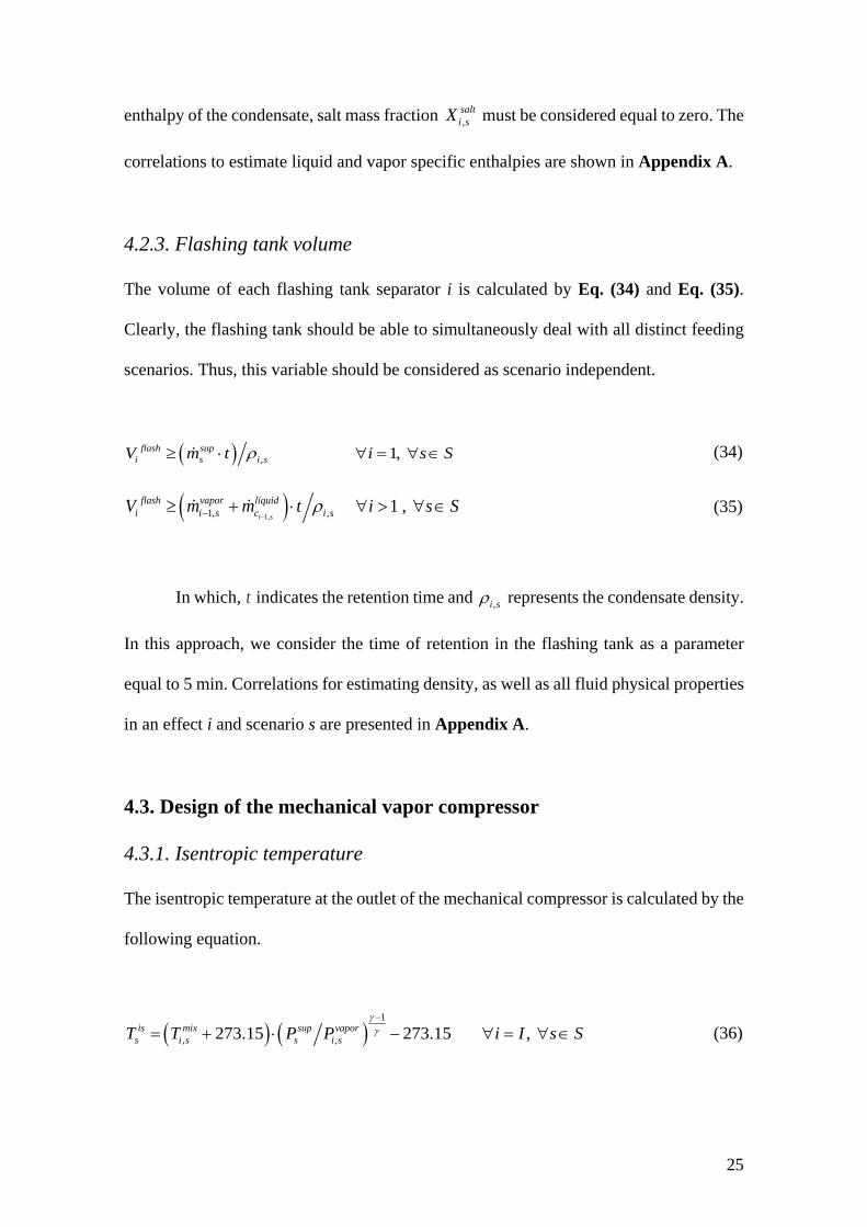
4.2.3. Flashing tank volume

The volume of each flashing tank separator i is calculated by Eq. (34) and Eq. (35).

Clearly, the flashing tank should be able to simultaneously deal with all distinct feeding

scenarios. Thus, this variable should be considered as scenario independent.

( ) , 1, ρ≥ ⋅ ∀∀ = ∈

flash supi s i s iV sm St (34)

( )1,1, , 1 , ρ−−≥ >+ ⋅ ∀ ∀ ∈

i s

flash vapor liquidi i s c i sm m iV t s S (35)

In which, t indicates the retention time and ,ρi s represents the condensate density.

In this approach, we consider the time of retention in the flashing tank as a parameter

equal to 5 min. Correlations for estimating density, as well as all fluid physical properties

in an effect i and scenario s are presented in Appendix A.

4.3. Design of the mechanical vapor compressor

4.3.1. Isentropic temperature

The isentropic temperature at the outlet of the mechanical compressor is calculated by the

following equation.

( ) ( )1

, ,273.15 273.15 , γγ−

= + ⋅ − ∀ = ∀ ∈is mix sup vapors i s s i sT T P P i I s S (36)

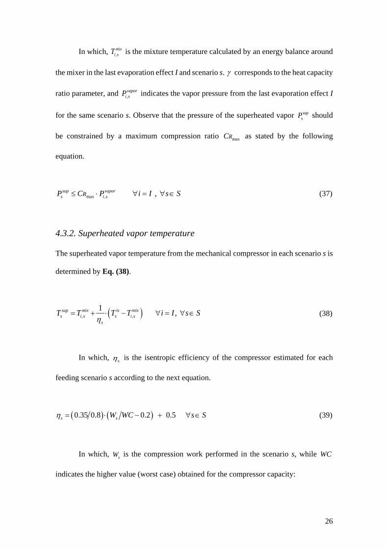
26

In which, ,mix

i sT is the mixture temperature calculated by an energy balance around

the mixer in the last evaporation effect I and scenario s. γ corresponds to the heat capacity

ratio parameter, and ,vapor

i sP indicates the vapor pressure from the last evaporation effect I

for the same scenario s. Observe that the pressure of the superheated vapor supsP should

be constrained by a maximum compression ratio maxRC as stated by the following

equation.

max , , ≤ = ∈⋅ ∀∀sup vapors i sRP C P I si S (37)

4.3.2. Superheated vapor temperature

The superheated vapor temperature from the mechanical compressor in each scenario s is

determined by Eq. (38).

( ), ,1 , η

= + ⋅ − ∀ = ∀ ∈sup mix is mixs i s s i s

s

T T T T i I s S (38)

In which, ηs is the isentropic efficiency of the compressor estimated for each

feeding scenario s according to the next equation.

( ) ( )0.35 0.8 0.2 0.5 η = ⋅ − + ∀ ∈s sW WC s S (39)

In which, sW is the compression work performed in the scenario s, while WC

indicates the higher value (worst case) obtained for the compressor capacity:

27

≥ ∀ ∈sWC W s S (40)

The Eq. (39) is valid for 0.5 0.85η≤ ≤s and 0.2 1sW WC≤ ≤ . These constraints

imply that the work performed by the compressor ( sW ) in a scenario s should be restricted

between 20% (with 50%sη = ) to 100% (with 5 8 %η =s ) of the nominal capacity of the

equipment (indicated by WC ). Note that the scenario-dependent variable sW should be

calculated to determine the distributions of energy consumption by the compressor and

its corresponding operational expenses; whereas WC should be used to estimate the

capital investment in the compressor.

4.3.3. Compression work

The compression work performed by the mechanical vapor compressor in each scenario

s is calculated by the following equation.

( ), , = ⋅ − ∀ = ∀ ∈

sup sup vapors s s i sW m H H i I s S (41)

In which, supsH and ,

vapori sH indicate vapor specific enthalpies that should be

estimated at superheated vapor temperature ( supsT ) and mixture temperature ( ,

mixi sT ) from

last evaporation effect, respectively. The correlations for these estimations are presented

in Appendix A.

28

4.3.4. Constraints on temperature and pressure

Constraints on the temperature and pressure at the compressor outlet should be used to

ensure the proper functioning of this equipment.

, , ≥ ∀ = ∀ ∈sup mixs i sT T i I s S (42)

, , ≥ ∀ = ∀ ∈sup vapors i sP P i I s S (43)

4.4. Design of the feeding preheater

4.4.1. Global energy balance

The global energy balance in the feeding preheater is stated by Eq. (44).

( ) ( ), , , , , , , , , ⋅ ⋅ − = ⋅ ⋅ − ∀ = ∀ ∈

i s

liquid condensate ideal freshwater feed feed feed feedc i s i s out s in s in s i s in sm Cp T T m Cp T T i I s S (44)

In which, ,freshwater

out sT represents the temperature of the produced freshwater in each

scenario s, while ,feed

in sT indicates the feeding temperature (shale gas flowback water). The

liquid specific heats of the condensate ( ,condensatei sCp ) and feed water ( ,

feedin sCp ) are estimated

by correlations shown in Appendix A.

4.4.2. Heat transfer area

The heat transfer area of the feeding preheater preheaterA is calculated by the Eq. (45).

Again, the heat transfer area should be considered as a scenario independent variable to

guarantee the suitability of this equipment under different feeding conditions (defined by

the scenarios set).

29

( ) ( ), , , , , ≥ ⋅ ⋅ − ⋅ ∀ = ∀ ∈

i s

preheater liquid condensate ideal freshwaterc i s i s out s s sMTDA m Cp T T U L i I s S (45)

In which, sU is the overall heat transfer coefficient estimated by Eq. (15),

considering the ideal temperature ,ideal

i sT . The logarithmic mean temperature difference

sMTDL in the preheater is calculated by Eq. (16), by considering:

1 , , 2 , , , and θ θ= − ∀ = ∀ ∈ = − ∀ ∈ideal feed freshwater feeds i s i s s out s in sT T i I s S T T s S (46)

4.5. Design specification for Zero-Liquid Discharge

The MEE-MVR system is designed to operate under ZLD condition. For this objective,

the brine salinity in the first evaporation effect should achieve its specification of design.

ZLD operation is ensured by the following constraint.

, 1, ≥ ∀ = ∀ ∈brine designi sS S i s S (47)

It should be emphasized that the inclusion of this constraint in the model restricts

the search space to solutions that meet a minimum salinity requirement designS for the brine

(e.g., brine salinity near salt saturation conditions). Obviously, lower costs are expected

for lesser brine salinity restrictions.

4.6. Stochastic objective function

The multiscenario stochastic model is optimized to obtain robust solutions, through the

expected value minimization of the objective distribution represented by the total

30

annualized cost. The stochastic objective function for minimization of the expected total

annualized cost ExpectedTAC of the MEE-MVR system can be expressed as follows:

( )1

,

1

1

min

. . Eq.(1) – Eq

.

(

46)= =

= ⋅ = ⋅ +

≥

∑ ∑S S

Expecteds

brine des

s s ss s

igns

TAC prob TAC prob CAPEX OPEX

S Ss t (48)

In which sprob represents the probability related to the occurrence of a specific

scenario s, and sTAC is the total annualized cost of the desalination system in this same

scenario. In this work, we consider equal probabilities of occurrence for all feeding water

scenarios. The total annualized cost distribution accounts for the capital investment in all

equipment (CAPEX ) used in the MEE-MVR system, and operational expenses in each

scenario s ( sOPEX ) related to the external steam source and electricity. Observe that the

capital investment is a scenario independent variable. On the other hand, operating

expenses should be defined by a stochastic function to capture all variability of the

system's energy consumption in the uncertain search space. This is because a different

system performance is obtained for each scenario s, while the equipment capacities should

be the same for all scenarios. The distributions of capital investment and operational costs

are given by Eq. (49) and Eq. (50), respectively.

( ) ( )

( )

2015

2003

1

=

⋅ ⋅ + ⋅ ⋅ +

= ⋅ ⋅ ⋅ ⋅ + ⋅ ⋅ ∑

evaporator compressorPO BM P PO BM P

flashIpreheater

POi BM P PO BM Pi

ac

C F F C F FCEPCICAPEX fCEPCI C F F C F F

(49)

electricit externy steams s

alsOPEX C W QC= ⋅ + ⋅ (50)

31

The annualization factor for the capital investment acf is calculated by the

following equation (Smith, 2005):

( ) ( )1

1 1 1y yacf fi fi fi

− = + − ⋅ + ⋅ (51)

In which, fi expresses the fractional interest rate per year in an amortization

period y. In Eq. (49), POC indicates the unitary equipment cost (in kUS$) calculated by

correlations presented in Turton et al. (2012) (flashing tank separators and feeding

preheater), and in Couper et al. (2010) (evaporator and mechanical vapor compressor).

BMF is the correction factor for the unitary equipment cost that correlates the operational

conditions to the materials of construction. In addition, the capital investment should be

corrected for the appropriate year with the CEPCI index (Chemical Engineering Plant

Cost Index). In Eq. (50), electricityC and steamC represent the parameters for the cost of

electricity and steam energy services, respectively.

5. Scenario generation: probability function and sampling

technique

In this section, we focus our attention on the generation of scenarios to properly describe

the uncertainty associated with the well data. Our stochastic modelling approach is based

on the assumption that the uncertain parameters (i.e., feed water flowrate and salinity)

can follow normal (Gaussian) correlated distributions. Thus, the uncertain parameters are

modelled through a probability multivariate distribution for which random values

(restricted by the distribution boundaries) are generated via Monte Carlo sampling

32

technique. As result, the uncertain parameters are depicted by a set of representative

scenarios with known probability of occurrence. As aforementioned, we assume the same

probability of occurrence for all feeding scenarios. Note that a given scenario corresponds

to a single sample of the uncertain parameters distribution (assumed as multivariate

normal). These explicit scenarios together with their associated probabilities are used as

input data for solving the optimization multiscenario model. Basically, our stochastic

approach admits the calculation of all scenario-dependent variables for each value

assumed by the random parameters, allowing constructing the total annualized cost

distribution.

Correlated scenarios are generated from a multivariate normal distribution via a

random number generator algorithm implemented in MATLAB based on the Mersenne

twister algorithm proposed by Matsumoto and Nishimura (1998). The probability density

function for correlated continuous random variables 1 2, , , dX X X , where each variable

has a univariate (or marginal) normal distribution is given by:

111 2 22

1( , , , ) exp ( ) ( )

(2 ) | |( )T

X df X X X X X

(52)

In which, µ is a d dimensional vector with the expected value of each random

variable ( iµ ), Σ is a d×d covariance matrix, and is the determinant of Σ . The diagonal

elements of Σ, which is a symmetric positive definite matrix, contain the variances for

each variable ( 2iσ ), while the off-diagonal elements of Σ contain the covariances between

variables ( ijσ ). It is worth to mention that a diagonal covariance matrix (i.e., all

covariances between variables are zero) implies that the random variables are not

correlated. The scenario generation method requires the attribution of the expected values

33

(nominal) and its variance for the uncertain parameters, in addition to their covariance

matrix. The expected values considered for generating each representative distribution of

uncertain parameters are shown in Table 2. The off-diagonal elements of the covariance

matrix can be calculated from the correlation matrix ijρ . Both matrices are related as

follows:

2 2ij

iji j

(53)

Hence, a symmetric correlation matrix is defined to describe the interactions

between the uncertain parameters. This symmetric matrix contains the information on

each pair of correlated random variables, by setting all non-diagonal elements with a

value between -1 and 1. It should be remarked that values ranging between -1 and 0

present negative correlation (which implies that one variable increases, while the other

linearly decreases), whereas values ranging between 0 and 1 are positively correlated

(which means that both variables linearly increase or decrease). If these factors assume

values equal to zero, the uncertain pair of variables are uncorrelated (Sabio et al., 2014).

Based on real information from shale plays, we assume that the uncertain

parameters have negative correlation. Typically, the salinity profile of the shale gas

flowback water shows a significant increase when the flowrate is reduced in the first two

weeks of well exploration (Acharya et al., 2011). The correlated feeding scenarios

generated with normal multivariate distributions, by considering different matrix

correlation factors are displayed in Fig. S1 of the supporting information. Observe that

the stochastic model is robust enough for dealing with scenarios generated by any

sampling technique and/or correlation. Regarding the number of scenarios, the model

accuracy generally increases as more scenarios are considered during the optimization.

34

Nevertheless, the CPU time to obtain a feasible solution is also increased due to

computational limitations (see Law and Kelton (2000) for more information about how

to obtain the best number of scenarios in stochastic programming models aimed at

optimizing the expected value of an objective function distribution).

6. Results and discussion

An illustrative case study is performed to evaluate the accurateness of the proposed

approach for synthesizing MEE-MVR desalination systems, under uncertainty of the

shale gas flowback water data. Fig. 1 depicts the superstructure proposed for the MEE-

MVR desalination plant of the flowback water from shale gas production. Firstly, we

present a comparison between the deterministic and stochastic solutions to emphasize the

importance of considering the proposed stochastic approach to solve this type of problem.

Then, we use the stochastic model to address the uncertainty related to the well data in

the shale gas production. Finally, sensitivity analysis is carried out to assess the optimal

system performance for distinct brine salinity conditions. The well data considered in this

example are based on real information obtained from important shale plays in the U.S.,

including Barnett and Marcellus (Acharya et al., 2011; Haluszczak et al., 2013; Hayes,

2009; Jiang et al., 2013; Slutz et al., 2012; Thiel and Lienhard V, 2014; Vidic et al., 2013;

Zammerilli et al., 2014) as shown in Table 1.

In this work, we consider expected mean (nominal) values of 8.68 kg s-1 (~750 m3

day-1) for the amount of shale gas flowback water—corresponding to the treating capacity

of the MEE-MVR plant—and 80 g kg-1 (80k ppm) for the flowback water salinity.

According to Slutz et al. (2012), the water amount required to complete each well—in

horizontal drilling and hydraulic fracturing processes—is in a range of 12 700−19 000

m3. However, this value can be very different for distinct wells (see Table 1). Thus, we

35

assume an expected mean value of 15 000 m3 for the amount of water required, and 25%

for the injected fluid that returns to surface as flowback water—during the first 15 days

from the beginning of well exploration—. In addition, we respect an annual scheduling

that comprises the exploration of 20 wells divided in fracturing crews (maximum

exploration of 3 wells at the same time) as proposed by Lira-Barragán et al. (2016).

Consequently, about 11 250 m3 of flowback water are recovered in the first 2 weeks of

the shale gas production start (~750 m3 day-1 or ~8.68 kg s-1). Note that, if a standard

deviation of 5% is considered from the mean value (15 000 m3), then ~95% of the

flowback water data will be between 13 500−16 500 m3 (and ~99.7% between 12 750−17

250 m3). In the same way, if standard deviations of 10% and 20% are considered, ~95%

of the flowback water data can be found in ranges of 12 000−18 000 m3 and 9 000−21

000 m3, respectively. With this in mind, we consider that standard deviations of 5%, 10%

and 20% are suitable to model the uncertainty associated with the amount of flowback

water. However, higher standard deviations must be considered for the flowback water

salinity due to the larger uncertainty related to these data (see Table 1). Hence, if a

standard deviation of 30% is considered from the expected mean value of the salt

concentration in the flowback water (80k ppm); ~95% of the data will be in the range of

32−128k ppm. Nevertheless, it should be highlighted that the brine discharge salinity

should be at least equal to 300 g kg-1 (300k ppm) to achieve ZLD operation (Han et al.,

2017).

Additional data include the operational limitations on the ideal temperature and

saturation pressure to prevent fouling and/or rusting problems in the evaporator

(horizontal-tube falling film/nickel), which should be lower than 100 ºC and 200 kPa,

correspondingly. A minimum temperature approach of 2 ºC is allowed for the superheated

vapor and condensate streams, as well as for vapor and brine concentrate streams. Note

36

that this minimum temperature approach is required to avoid temperature crossover in the

effects of evaporation. Moreover, a minimum pressure and temperature drops between

two successive effects are considered equal to 0.1 kPa and 0.1 ºC, respectively. The heat

capacity ratio γ is considered to be equal to 1.33, while the maximum compression ratio

maxRC is restricted to 3 for the mechanical compressor design (centrifugal/carbon steel).

Cost data comprises the electricity—850.51 US$ (kW year)-1—and steam—418.8 US$

(kW year)-1—prices. An annualized cost factor (fac) of 0.16 is considered for capital cost

estimations, which corresponds to an interest rate of 10% over an amortization period of

10 years. The problem data considered for the case study are summarized in Table 2.

6.1. Deterministic vs stochastic solution

Initially, we contrast the optimal solutions obtained from the deterministic and stochastic

approaches for assessing the impact of uncertainty on the MEE-MVR system

performance. Thus, we firstly solve the deterministic model through the minimization of

the process total annualized cost. It should be highlighted that the deterministic model

can be easily obtained from the proposed stochastic approach, by considering one single

scenario. In this case, the optimization scenario should correspond to the expected mean

(nominal) values for the well data (i.e., 80 g kg-1 for the flowback water salinity and 8.68

kg s-1 for the flowrate). The deterministic model allows obtaining an optimal system

configuration and corresponding operational conditions. Afterwards, equipment

capacities obtained from this method—including evaporator and preheater heat transfers

areas, flashing tanks volumes and compressor capacity—are fixed in the stochastic model

to evaluate the system performance under distinct feeding scenarios.

The optimal MEE-MVR desalination system obtained by the deterministic

approach is composed of two evaporator effects with heat transfers areas equal to 59.46

37

m2 (7819.12 kW) and 178.36 m2 (7674.59 kW), in addition to a mechanical vapor

compressor with capacity of 457 kW ( 0.85η = ). Furthermore, a feed preheater with heat

transfer area of 71.47 m2 (1469.53 kW), and flashing tanks with volumes of 1.24 m3 and

2.77 m3 are also needed in the system. Fig. 3 displays the optimal MEE-MVR system

configuration and operational conditions obtained by the deterministic model. With this

configuration, the system requires 177.21 kW of additional energy from the external

steam source. The total annualized cost obtained for the deterministic case is equal to

1055 kUS$ year-1, comprising 463 kUS$ year-1 related to operational expenses (steam

and electricity consumption) and 592 kUS$ year-1 associated with capital investment. It

should be noted that the system operates at ZLD operation (salt concentration in the brine

discharge equal to 300 g kg-1). Under this condition, a freshwater production ratio of 6.37

kg s-1 is achieved by the desalination plant. This value corresponds to ~73.3% of

condensate (freshwater) recovery. The freshwater production cost is equal to 5.25 US$

per cubic meter (~0.02 US$ gallon-1), of which ~43% are related to energy consumption.

Note that the cost of water disposal in Class II saline water injection sites (conventional

deep-well injection) are between ~8−25 US$ per cubic meter (~0.03−0.08 US$ gallon-

1)—cost for water disposal in locally available wells in Barnett shale play—(Acharya et

al., 2011). These values emphasize the economic viability of the proposed ZLD

desalination system for the shale gas flowback water.

Hereafter, we perform the stochastic optimization by fixing the equipment

capacities provided by the deterministic solution. In this case, feed data uncertainty is

described via 100 different feeding scenarios generated by sampling technique. For this

purpose, it is assumed a normal correlated distribution with 10% of standard deviation

from the mean values (8.68 kg s-1 and 80 g kg-1). In addition, we consider a correlation

matrix factor of -0.8 (which means that the uncertain parameters are strongly correlated).

38

Observe that the number of scenarios is chosen as the smallest number of scenarios from

which no significant differences is found between successive optimizations.

The stochastic solution obtained by considering the deterministic configuration

presents an expected total annualized cost equal to 1129 kUS$ year-1. This amount

corresponds to an increment of ~7% in comparison with the deterministic total annualized

cost. It is emphasized that the total process cost is increased due to the adjustment of the

operational conditions needed to enable the operation of the MEE-MVR system in all

scenarios. Clearly, the MEE-MVR system has the same capital investment than the

deterministic solution (592 kUS$ year-1). However, the operational expenses are different

for each feeding scenario. For the first scenario, we report operational expenses of 286

kUS$ year-1, representing a decrease of ~38.2% in relation to the one obtained for the

deterministic approach. In this scenario, the desalination system only requires 336.15 kW

of electricity—which implies that the mechanical vapor compressor operates at 73.6% of

the nominal equipment capacity with efficiency of 0.73η = —with no need for external

steam.

Although some feeding scenarios present lower operating costs, more than 50%

of them exhibit higher values than the one obtained in the deterministic solution. For

instance, scenarios 49 and 66 show operational expenses equal to 479 kUS$ year-1 and

572 kUS$ year-1, respectively. Even further increased values are obtained for scenarios

81 and 90 (705 kUS$ year-1 and 803 kUS$ year-1, respectively). Note that the scenarios

49 and 66 consume 214.89 kW and 438.29 kW from the external energy source,

correspondingly. Scenarios 81 and 90 use 755.27 kW and 988.97 of steam, respectively.

Yet, the above-mentioned scenarios need the same amount of electricity (457 kW), which

indicates that the compressor is working on its maximum nominal capacity. Scenario 100

presents the worst case for these expenses, presenting operational costs equal to 1386

39

kUS$ year-1. This value represents an increase of ~200% in comparison with the

deterministic solution. In the last scenario, energy consumption comprises 457 kW (with

0.85η = ) of electricity and 2381.28 kW of steam. The operational expenses distribution

in the uncertain search space is illustrated in Fig. S2 of the supporting information. The

energy consumption distribution throughout the distinct feeding scenarios is displayed in

Fig. 4. We highlight that all scenarios operate at ZLD condition. For convenience,

scenarios are sorted by ascending order of feed flowrate inlet data.

First and last scenarios show a similar freshwater production cost of ~6.8 US$ per

cubic meter (~0.03 US$ gallon-1), which corresponds to an increase of ~30% in

comparison with the deterministic solution. Fig. 5 depicts the freshwater cost distribution

obtained via stochastic approach throughout the different feeding scenarios. For allowing

comparisons with the deterministic solution, the freshwater production cost is estimated

by considering the operating expenses and capital investment individually for each

scenario. Therefore, energy consumption and respective operating expenses and

freshwater production costs can be prohibitive for some feeding scenarios. This is due to

the weak system performance under feeding conditions that have not been considered

during its design task. For this reason, we stress the importance of the stochastic design

to provide all system flexibility under process parameters variability. The stochastic

MEE-MVR system design is shown in the following section.

6.2. Stochastic system design and risk analysis

For the stochastic optimization of the MEE-MVR system, we consider the previous

expected mean values (8.68 kg s-1 and 80 g kg-1), and standard deviations of 10% for both

feed water flowrate and salt concentration. Again, feed data uncertainty is described via

100 distinct scenarios correlated by a matrix correlation factor of -0.8. The scenarios are

40

sorted by ascending order of feed flowrate inlet data. Fig. 6 shows the correlated feeding

scenarios generated with a marginal normal multivariate distribution. In this case, the

optimal MEE-MVR system obtained is composed of two evaporator effects with heat

transfers areas of 66.31 m2 and 198.93 m2; in addition to a mechanical vapor compressor

with capacity of 498.11 kW, and a feed preheater with heat transfer area of 72.62 m2.

Furthermore, two flashing tanks are also required in the system with volumes equal to

1.29 m3 and 2.77 m3, respectively. Fig. 7 displays the optimal MEE-MVR system

configuration obtained by the proposed stochastic model. Note that the total heat transfer

area and compressor capacity are both increased by ~9%, in comparison with the optimal

solution provided by the earlier deterministic approach. We emphasize that the equipment

increment is needed to ensure the optimal system performance in all considered scenarios.

The optimal solution for the MEE-MVR system presents an expected total annualized

cost equal to 1110 kUS$ year-1, from which 637 kUS$ year-1 are related to the capital

investment.

Distributions of energy consumption and corresponding operational expenses

throughout the distinct feeding scenarios are displayed in Fig. S3 and Fig. S4 of the

supporting information. In the latter distribution, the first scenario only consumes

electricity (330.3 kW). For this reason, this scenario presents the lowest operating

expenses (280.9 kUS$ year-1). However, other scenarios require energy consumption

much more elevated than the first one. For example, the scenarios 81 and 90 need 498.11

kW (each one) of electricity; and, 366.52 kW and 541.71 kW of external steam,

respectively. Consequently, these scenarios exhibit operational expenses equal to 577.14

kUS$ year-1 and 650.52 kUS$ year-1, correspondingly. It should be noted that the last

scenario shows the highest energy consumption (1578.18 kW of steam and 498.11 of

electricity) and related operating costs (1084.59 kUS$ year-1).

41

From scenario 45 onwards, the MEE-MVR system demands all maximum

nominal capacity of the mechanical vapor compressor (498.11 kW). Moreover, the

desalination system also starts consuming external steam from this scenario, as shown in

Fig. S3 (see supporting information). It is worth to mention that the desalination system

obtained by the stochastic approach also achieves the ZLD condition in all considered

scenarios. Though, the first scenario attains the lowest freshwater production ratio (4.08

kg s-1). As expected, this scenario shows the highest freshwater production cost that is

equal to 8.63 US$ per cubic meter (~0.033 US$ gallon-1). On the other hand, the highest

amount of produced freshwater is obtained by the last scenario (9.22 kg s-1). For the latter,

the freshwater cost is equal to 3.82 US$ per cubic meter (~0.015 US$ gallon-1). Here, the

freshwater production cost is estimated by means of the expected total annualized cost.

Fig. 8 displays the distributions for the freshwater production cost and produced

freshwater throughout the distinct feeding scenarios.

Cumulative probability curves for the system economic performance (considering

weakly and strongly correlated uncertain parameters) are depicted in Fig. 9 and Fig. 10,

respectively. In both cases, standard deviations of 5%, 10% and 20% from the expected

mean values are considered for the generation of the uncertain scenarios. In these curves,

the vertical axis indicates the probability of achieving an economic performance lesser or

equal to a target value presented in the horizontal axis. For instance, if the decision-maker

targets a maximum value for the process total annualized cost of 1200 kUS$ year-1, Fig.

9 shows that the 5% curve has ~97% of probability of achieving this goal; whereas the

10% and 20% curves present lower probabilities of ~90% and ~75%, respectively. If a

more ambitious objective of 1100 kUS$ year-1 is targeted for the economic performance,

the probabilities are significantly reduced to ~88% (5% curve), ~68% (10% curve) and

~48% (20% curve).

42

If the uncertain parameters are strongly correlated as considered in Fig. 10, the

probabilities of attaining the more conservative goal (1200 kUS$ year-1) are reduced for

all standard deviations (5%, 10% and 20% curves). In this case, the probabilities are equal

to ~96% (5% curve), ~87% (10% curve) and ~60% (20% curve), correspondingly. A

thorough examination of both curves reveals that the consideration of uncertain

parameters with higher standard deviations involves riskier decision-making. It should be

noted that higher standard deviation curves show lower probability of reaching a certain

economic performance. More precisely, the 20% curve in Fig. 9 presents ~12% of

probability of exceeding a target cost of 1311 kUS$ year-1, while this probability is null

for the 5% curve.

Fig. 9 and Fig. 10 also display the minimum and maximum values for the total

annualized cost, as well as the expected economic performance obtained for all standards

deviations. In Fig. 9, the expected total annualized cost is increased by ~7.9% between

the optimal solutions found for 5% (1066 kUS$ year-1) and 20% (1150 kUS$ year-1) of

standard deviations. For the 5% curve, the upper bound for the economic performance is

~35% higher than its corresponding minimum value. Instead, the 20% standard deviation

curve presents ~181.3% of increase in the total annualized cost when its extreme solutions

are compared. Thus, the solutions present worse expected economic performance, and

more variability in the total annualized cost as the uncertainty level is increased during

the system design. Note that in Fig. 10, the expected total annualized cost for the 20%

standard deviation (1200 kUS$ year-1) is ~12% higher than the optimal solution obtained

for 5% of standard deviation (1070 kUS$ year-1).

Finally, even worse expected performance and higher variability in the total

annualized cost are verified as the correlation level is increased between the uncertain

parameters. This is because the correlated parameters assume simultaneously the lowest

43

and highest values of the uncertain search space, which leads to extreme scenarios. We

report that other risk management metrics have been used to solve this problem, including

the worst case for the total annualized cost and downside risk. In these cases, multi-

objective optimizations have been performed through the minimization of the expected

value and the referred metrics. However, the obtained Pareto curves did not exhibit

significant trade-offs between solutions. Hence, variations in the upper bound (ε -

constraint) for these risk metrics (worst case and downside risk) did not change the

expected value for the total annualized cost.

The proposed NLP-based model for both deterministic and stochastic

optimizations of the MEE-MVR desalination system has been implemented in GAMS

(version 24.7.4), and optimized by the interior-point solver IPOPT (Wächter and Biegler,

2006) with CPLEX as sub-solver. A personal computer with an Intel Core i5-2520M 2.5

GHz processor and 8 GB RAM running Windows 10 has been used for solving all case

studies. The CPU time for the deterministic optimization has not exceeded 1 s, while the

stochastic ones have required 10 to 15 s to get optimal solutions. In the deterministic case,

the mathematical model encompasses 93 continuous variables, 105 constraints with 292

Jacobian (non-zeros) elements, of which 106 are nonlinear. Instead, the stochastic

mathematical model contains 7 320 continuous variables, 9 114 constraints with 26 131

Jacobian (non-zeros) elements, of which 10 303 are nonlinear.

6.3. Sensitivity analysis

A straightforward sensitivity analysis is carried out to evaluate the energy and economic

performances of the MEE-MVR system under different discharge brine salinities. In this

way, we consider several ZLD conditions defined by the brine salinity ranging between

200 and 320 g kg-1 1 (200–320 k ppm). The stochastic optimizations are performed by

44

considering the same expected mean values for inlet feed water salinity and flowrate (8.68

kg s-1 and 80 g kg-1), as well as the same standard deviations (10%) and matrix correlation

factor (-0.8) for the generation of the uncertain parameters. Once again, we consider an

uncertain search space composed by 100 distinct feeding scenarios. Box and whisker

plots for energy consumption and total annualized cost according to discharge brine

salinity are displayed in Fig. S5 and Fig. S6 (supporting information), respectively.

These plots indicate that the total energy consumption (related to electricity and steam)

and total annualized cost (including capital investment and operational expenses) are

more elevated as higher ZLD constraints are imposed on the system design. It should be

highlighted that for the same inlet feed conditions given by the scenarios, higher

restrictions on ZLD conditions imply greater brine concentrations.

The expected total energy consumption for the brine salinity of 200 g kg−1 is equal

to 572 kW, whereas the ZLD constraint of 320 g kg−1 requires 657 kW of energy. This

value represents an increase of ~15% in comparison with the first solution. In accordance

with these results, expected total annualized cost is increased by ~21% between the brine

salinity conditions of 200 g kg−1 (945 kUS$ year-1) and 320 g kg−1 (1144 kUS$ year-1).

The distributions of energy consumption and total annualized cost are also shown in Fig.

S5 and Fig. S6. As can be observed in Fig. S6, 50% of the solutions for the system

economic performance under brine salinity constraint of 250 g kg−1 are in the range of

945−1070 kUS$ year-1 (quartiles 1 and 3). For this case, minimum and maximum values

for the total annualized cost distribution are equal to 839 kUS$ year-1 and 1571 kUS$

year-1, respectively. The expected mean value for the total annualized cost is equal to

1029 kUS$ year-1, while the median is 1005 kUS$ year-1. It is important to emphasize

that the proposed stochastic multiscenario approach, allows obtaining robust solutions

when accounting for parameter uncertainty. Such system performance robustness cannot

45

be ensured by a deterministic model, since it is not able to provide the distributions for

the energy consumption and process costs.

7. Conclusions

A new stochastic optimization model for the design of ZLD desalination systems under

uncertainty is introduced in this work. The model is based on a multistage superstructure

defined by multiple-effect evaporation process with heat integration and mechanical

vapor recompression (MEE-MVR). The MEE-MVR system is especially developed for

the desalination of high-salinity flowback water from shale gas production. Our main goal

is to enhance energy efficiency of the process through the reduction of brine discharges,

while accounting for distinct water feeding scenarios. To achieve this objective, we define

the outflow brine salinity near to salt saturation as a design constraint to reach ZLD

operation. Important improvements in the process are implemented, including the use of

an external energy source to avoid oversized equipment. Additionally, we consider the

compressor isentropic efficiency as a variable throughout the different scenarios. This

novelty allows obtaining a more precise and robust system operational performance. In

this new approach, feed water (i.e., shale gas flowback water) salinity and flowrate are

both treated as uncertain design parameters. These uncertain parameters are

mathematically modelled as a set of correlated scenarios with given probability of

occurrence. The feeding scenarios are described by multivariate normal distribution

generated via sampling technique with symmetric correlation matrix. The resulting

stochastic multiscenario NLP-based model is optimized in GAMS, through the

minimization of the expected total annualized cost.

An illustrative case study is performed to evaluate the capabilities of the proposed

new approach for the design of MEE-MVR desalination systems under uncertainty of

46

shale gas flowback water data. Firstly, we compare the optimal solutions obtained from

the deterministic and stochastic models for assessing the impact of uncertainty on the

energy and economic system performances. In this case, our results show that the energy

consumption and corresponding operational expenses and freshwater production costs

can be prohibitive for some scenarios. This is a result of the weak system performance

under feeding water conditions that have not been accounted during the MEE-MVR

design task. Therefore, it is clear that the stochastic design approach should be considered

to provide system flexibility under variability of process uncertain parameters.

Afterwards, we carry out the stochastic optimization of the MEE-MVR

desalination system. This is an innovative approach, since it allows obtaining the

distributions of energy consumption and corresponding operational expenses throughout

the distinct feeding scenarios. Still, we construct cumulative probability curves to

appraise the financial risk associated with uncertain space for distinct standard deviations

of mean values. A thorough inspection of these curves indicates that the consideration of

uncertain parameters with higher standard deviations involves riskier decision-making.

The latter can be explained by the lower probability of reaching a certain economic

performance, as depicted by the curves with higher standard deviation.

Lastly, a straightforward sensitivity analysis is performed to show the optimal

system performance for distinct outflow brine salinity conditions. We highlight that the

proposed stochastic multiscenario methodology leads to better energy and economic

performance solutions than a deterministic method. This is due to the fact that

deterministic models cannot provide the distributions for energy consumption and process

costs. For this reason, our approach represents a useful tool for supporting decision-

makers towards the implementation of more robust and reliable ZLD desalination systems

for treatment of shale gas flowback water.

47

Acknowledgements

This project has received funding from the European Union’s Horizon 2020

Research and Innovation Programme under grant agreement No. 640979.

48

Nomenclature

Roman letters

A Heat transfer area, m2

BPE Boiling point elevation, ºC

electricityC Parameter for electricity cost, US$ (kW year)-1

steamC Parameter for steam cost, US$ (kW year)-1

CAPEX Capital Expenditures, kUS$ year-1

Cp Specific heat, kJ (kg ºC)-1

POC Cost of equipment unit, kUS$

maxRC Maximum compression ratio

acf Factor of annualized capital cost

BMF Correction factor for the capital cost

fi Fractional interest rate per year

PF Parameter for the capital cost estimation

H Specific enthalpy, kJ kg-1

MTDL Logarithmic mean temperature difference

m Mass flowrate, kg s-1

feedm Stochastic parameter for feeding mass flowrate, kg s-1

feedm Expected mean (nominal) value for feeding mass flowrate, kg s-1

OPEX Operational Expenses, kUS$ year-1

P Pressure, kPa

prob Probability

min∆P Minimum pressure approach, kPa

49

Q Heat flow, kW

S Salinity, g kg-1

feedS Stochastic parameter for feeding water salinity, g kg-1

feedS Expected mean (nominal) value for feeding water salinity, g kg-1

T Temperature, ºC

t Retention time in the flash tanks, min

TAC Total annualized cost, kUS$ year-1

min∆T Minimum temperature approach, ºC

U Overall heat transfer coefficient, kW m-2K-1

V Volume, m3

saltX Salt mass fraction

W Compression work, kW

WC Compressor capacity, kW

y Number of years

Subscripts

i Evaporator effects

in Inlet condition

out Outlet condition

s Scenarios

Superscript

cv Condensate (or Distillate) vapor

is Isentropic

50

mix Mixture

S Sensible heat

sat Saturated vapor

sup Superheated vapor

Acronyms

BPE Boiling Point Elevation

CEPCI Chemical Engineering Plant Cost Index

EC Evaporative Crystallization

GAMS General Algebraic Modelling System

MEE Multiple-Effect Evaporation

MD Membrane Distillation

MSF Multistage Flash Distillation

MVR Mechanical Vapor Recompression

NEA Non-Equilibrium Allowance

NLP Nonlinear Programming

RO Reverse Osmosis

SEE Single-Effect Evaporation

TVR Thermal Vapor Recompression

ZLD Zero-Liquid Discharge

Greek letters

γ Heat capacity ratio

η Isentropic efficiency

θ Temperatures difference, ºC

51

κ Thermal conductivity, kW (m K)-1

λ Latent heat of vaporization, kJ kg-1

µ Viscosity, kg (m s)-1

ρ Density, kg m-3

σ Standard deviation

52

References

Abraham, R., Mani, A., 2015. Heat transfer characteristics in horizontal tube bundles for

falling film evaporation in multi-effect desalination system. Desalination 375, 129–

137. doi:10.1016/j.desal.2015.06.018

Acharya, H.R., Henderson, C., Matis, H., Kommepalli, H., Moore, B., Wang, H., 2011.

Cost effective recovery of low-TDS frac flowback water for re-use. Glob. Res. 1–

100.

Al-Mutaz, I.S., Wazeer, I., 2014. Comparative performance evaluation of conventional

multi-effect evaporation desalination processes. Appl. Therm. Eng. 73, 1194–1203.

doi:10.1016/j.applthermaleng.2014.09.025

Boo, C., Lee, J., Elimelech, M., 2016. Omniphobic polyvinylidene fluoride (PVDF)

membrane for desalination of shale gas produced water by membrane distillation.

Environ. Sci. Technol. 50, 12275–12282. doi:10.1021/acs.est.6b03882

Carrero-Parreño, A., Onishi, V.C., Salcedo-Díaz, R., Ruiz-Femenia, R., Fraga, E.S.,

Caballero, J.A., Reyes-Labarta, J.A., 2017. Optimal pretreatment system of

flowback water from shale gas production. Ind. Eng. Chem. Res. 56, 4386–4398.

doi:10.1021/acs.iecr.6b04016

Chen, H., Carter, K.E., 2016. Water usage for natural gas production through hydraulic

fracturing in the United States from 2008 to 2014. J. Environ. Manage. 170, 152–

159. doi:10.1016/j.jenvman.2016.01.023

Chen, J.J.J., 1987. Comments on improvements on a replacement for the logarithmic

mean. Chem. Eng. Sci. 42, 2488–2489. doi:10.1016/0009-2509(87)80128-8

Cho, H., Choi, Y., Lee, S., Sohn, J., Koo, J., 2016. Membrane distillation of high salinity

wastewater from shale gas extraction: effect of antiscalants. Desalin. Water Treat.

57, 26718–26729. doi:10.1080/19443994.2016.1190109

53

Chung, H.W., Swaminathan, J., Warsinger, D.M., Lienhard V, J.H., 2016. Multistage

vacuum membrane distillation (MSVMD) systems for high salinity applications. J.

Memb. Sci. 497, 128–141. doi:10.1016/j.memsci.2015.09.009

Cooper, J., Stamford, L., Azapagic, A., 2016. Shale gas: A review of the economic,

environmental, and social sustainability. Energy Technol. 4, 772–792.

doi:10.1002/ente.201500464

Couper, J.R., Penney, W.C., Fair, J.R., Walas, S.M., 2010. Chemical process equipment,

selection and design, Second Edition, USA: Elsevier.

EIA, 2016a. Annual Energy Outlook 2016 with Projections to 2040. Washington, DC:

U.S. Energy Information Administration, 2016.

EIA, 2016b. International Energy Outlook 2016. Washington, DC: U.S. Energy

Information Administration, 2016.

El-Dessouky, H.T., Ettouney, H.M., 1999. Multiple-effect evaporation desalination

systems: Thermal analysis. Desalination 125, 259–276. doi:10.1016/S0011-

9164(99)00147-2

European Commission, 2016. Eurostat.

Gao, J., You, F., 2015. Deciphering and handling uncertainty in shale gas supply chain

design and optimization: Novel modeling framework and computationally efficient

solution algorithm. AIChE J. 61, 3739–3755. doi:10.1002/aic.15032

Ghanbari, E., Dehghanpour, H., 2016. The fate of fracturing water: A field and simulation

study. Fuel 163, 282–294. doi:10.1016/j.fuel.2015.09.040

Haluszczak, L.O., Rose, A.W., Kump, L.R., 2013. Geochemical evaluation of flowback

brine from Marcellus gas wells in Pennsylvania, USA. Appl. Geochemistry 28, 55–

61. doi:10.1016/j.apgeochem.2012.10.002

Hammond, G.P., O’Grady, Á., 2017. Indicative energy technology assessment of UK

54

shale gas extraction. Appl. Energy 185, 1907–1918.

doi:10.1016/j.apenergy.2016.02.024

Han, D., He, W.F., Yue, C., Pu, W.H., 2017. Study on desalination of zero-emission

system based on mechanical vapor compression. Appl. Energy 185, 1490–1496.

doi:10.1016/j.apenergy.2015.12.061

Hayes, T., 2009. Sampling and analysis of water streams associated with the development

of Marcellus shale gas. Rep. by Gas Technol. Institute, Des Plaines, IL, Marcellus

Shale Coalit. 10.

Huang, L., Fan, H., Xie, H., Huang, Z., 2016. Experimental study of treatment processes

for shale gas fracturing flowback fluid in the eastern Sichuan Basin. Desalin. Water

Treat. 57, 24299–24312. doi:10.1080/19443994.2016.1141714

Jacquet, J.B., 2014. Review of risks to communities from shale energy development.

Environ. Sci. Technol. 48, 8321–8333. doi:10.1021/es404647x

Jang, E., Jeong, S., Chung, E., 2017. Application of three different water treatment

technologies to shale gas produced water. Geosystem Eng. 20, 104–110.

doi:10.1080/12269328.2016.1239553

Jiang, Q., Rentschler, J., Perrone, R., Liu, K., 2013. Application of ceramic membrane

and ion-exchange for the treatment of the flowback water from Marcellus shale gas

production. J. Memb. Sci. 431, 55–61. doi:10.1016/j.memsci.2012.12.030

Law, A.M., Kelton, W.D., 2000. Simulation Modeling and Analysis, 3rd ed. New York:

McGraw Hill, 2000.

Lira-Barragán, L.F., Ponce-Ortega, J.M., Guillén-Gosálbez, G., El-Halwagi, M.M., 2016.

Optimal water management under uncertainty for shale gas production. Ind. Eng.

Chem. Res. 55, 1322–1335. doi:10.1021/acs.iecr.5b02748

Matsumoto, M., Nishimura, T., 1998. Mersenne twister: a 623-dimensionally

55

equidistributed uniform pseudo-random number generator. ACM Trans. Model.

Comput. Simul. 8, 3–30. doi:10.1145/272991.272995

Michel, M.M., Reczek, L., Granops, M., Rudnicki, P., Piech, A., 2016. Pretreatment and

desalination of flowback water from the hydraulic fracturing. Desalin. Water Treat.

57, 10222–10231. doi:10.1080/19443994.2015.1038588

Onishi, V.C., Carrero-Parreño, A., Reyes-Labarta, J.A., Fraga, E.S., Caballero, J.A.,

2017a. Desalination of shale gas produced water: A rigorous design approach for

zero-liquid discharge evaporation systems. J. Clean. Prod. 140, 1399–1414.

doi:10.1016/j.jclepro.2016.10.012

Onishi, V.C., Carrero-Parreño, A., Reyes-Labarta, J.A., Ruiz-Femenia, R., Salcedo-Díaz,

R., Fraga, E.S., Caballero, J.A., 2017b. Shale gas flowback water desalination:

Single vs multiple-effect evaporation with vapor recompression cycle and thermal

integration. Desalination 404, 230–248. doi:10.1016/j.desal.2016.11.003

Qiu, Q., Zhu, X., Mu, L., Shen, S., 2015. Numerical study of falling film thickness over

fully wetted horizontal round tube. Int. J. Heat Mass Transf. 84, 893–897.

doi:10.1016/j.ijheatmasstransfer.2015.01.024

Sabio, N., Pozo, C., Guillén-Gosálbez, G., Jiménez, L., Karuppiah, R., Vasudevan, V.,

Sawaya, N., Farrell, J.T., 2014. Multiobjective optimization under uncertainty of the

economic and life-cycle environmental performance of industrial processes. AIChE

J. 60, 2098–2121. doi:10.1002/aic.14385

Sahinidis, N. V., 2004. Optimization under uncertainty: state-of-the-art and opportunities.

Comput. Chem. Eng. 28, 971–983. doi:10.1016/j.compchemeng.2003.09.017

Shaffer, D.L., Arias Chavez, L.H., Ben-Sasson, M., Romero-Vargas Castrillón, S., Yip,

N.Y., Elimelech, M., 2013. Desalination and reuse of high-salinity shale gas

produced water: drivers, technologies, and future directions. Environ. Sci. Technol.

56

47, 9569–9583. doi:10.1021/es401966e

Shen, S., Mu, X., Yang, Y., Liang, G., Liu, X., 2015. Experimental investigation on heat

transfer in horizontal-tube falling-film evaporator. Desalin. Water Treat. 56, 1440–

1446. doi:10.1080/19443994.2014.949604

Slutz, J., Anderson, J., Broderick, R., Horner, P., 2012. Key shale gas water management

strategies: an economic assessment tool. SPE/APPEA Int. Conf. Heal. Safety,

Environ. Oil Gas Explor. Prod. Perth, Aust. Sept. 2012.

Smith, R.M., 2005. Chemical Process Design and Integration. Second Edition, England,

John Wiley and Sons Ltd.

Stephenson, T., Valle, J.E., Riera-Palou, X., 2011. Modeling the relative GHG emissions

of conventional and shale gas production. Environ. Sci. Technol. 45, 10757–10764.

doi:10.1021/es2024115

Thiel, G.P., Lienhard, J.H., 2014. Treating produced water from hydraulic fracturing:

Composition effects on scale formation and desalination system selection.

Desalination 346, 54–69. doi:10.1016/j.desal.2014.05.001

Thu, K., Kim, Y.-D., Shahzad, M.W., Saththasivam, J., Ng, K.C., 2015. Performance

investigation of an advanced multi-effect adsorption desalination (MEAD) cycle.

Appl. Energy 159, 469–477. doi:10.1016/j.apenergy.2015.09.035

Tong, T., Elimelech, M., 2016. The global rise of zero liquid discharge for wastewater

management: drivers, technologies, and future directions. Environ. Sci. Technol. 50,

6846–6855. doi:10.1021/acs.est.6b01000

Turton, Bailie, R.C., Whiting, W.B., 2012. Analysis , Synthesis , and Design of Chemical

Processes, fourth ed.

Vengosh, A., Jackson, R.B., Warner, N., Darrah, T.H., Kondash, A., 2014. A critical

review of the risks to water resources from unconventional shale gas development

57

and hydraulic fracturing in the United States. Environ. Sci. Technol. 48, 8334–8348.

doi:10.1021/es405118y

Vengosh, A., Warner, N., Jackson, R., Darrah, T., 2013. The effects of shale gas

exploration and hydraulic fracturing on the quality of water resources in the United

States. Procedia Earth Planet. Sci. 7, 863–866. doi:10.1016/j.proeps.2013.03.213

Vidic, R.D., Brantley, S.L., Vandenbossche, J.M., Yoxtheimer, D., Abad, J.D., 2013.

Impact of shale gas development on regional water quality. Science (80) 340,

1235009–1235009. doi:10.1126/science.1235009

Wächter, A., Biegler, L.T., 2006. On the implementation of an interior-point filter line-

search algorithm for large-scale nonlinear programming. Math. Program. 106, 25–

57. doi:10.1007/s10107-004-0559-y

Xiong, B., Zydney, A.L., Kumar, M., 2016. Fouling of microfiltration membranes by

flowback and produced waters from the Marcellus shale gas play. Water Res. 99,

162–170. doi:10.1016/j.watres.2016.04.049

Yang, L., Grossmann, I.E., Manno, J., 2014. Optimization models for shale gas water

management. AIChE J. 60, 3490−3501. doi:10.1002/aic.14526

Zammerilli, A., Murray, R.C., Davis, T., Littlefield, J., 2014. Environmental impacts of

unconventional natural gas development and production DOE/NETL-2014/1651,

800, 553−7681.

Zhang, X., Sun, A.Y., Duncan, I.J., 2016. Shale gas wastewater management under

uncertainty. J. Environ. Manage. 165, 188–198. doi:10.1016/j.jenvman.2015.09.038

58

List of Figure Captions

Fig. 1. General superstructure proposed for the MEE-MVR desalination plant of

flowback water from shale gas production. This figure is adapted from Onishi et al.

(2017b).

Fig. 2. Decision variables for the optimization of: (a) single-stage compressor; and, (b)

effect i of the horizontal falling film evaporator coupled to flashing tank i in the MEE-

MVR system.

Fig. 3. Optimal configuration and operational conditions obtained for the multiple-effect

evaporation system with mechanical vapor recompression (MEE-MVR) through the

deterministic approach.

Fig. 4. Energy consumption distribution throughout the different feeding scenarios,

obtained via stochastic approach with fixed equipment capacities as provided by the

deterministic solution.

Fig. 5. Freshwater cost distribution throughout the different feeding scenarios, obtained

via stochastic approach with fixed equipment capacities as provided by the deterministic

solution.

Fig. 6. Correlated feeding scenarios generated with marginal normal distribution,

considering matrix correlation of - 0.8 and standard deviation of 10% from expected mean

values.

Fig. 7. Optimal MEE-MVR system configuration obtained by the proposed stochastic

modelling approach.

Fig. 8. Distributions of freshwater production cost and produced freshwater obtained by

the stochastic model throughout the distinct feeding scenarios.

Fig. 9. Cumulative probability curves for the system economic performance under

consideration of weakly correlated uncertain parameters (matrix correlation factor of 0.1).

59

Fig. 10. Cumulative probability curves for the system economic performance under

consideration of strongly correlated uncertain parameters (matrix correlation of 0.9).

60

Appendix A. Correlations for estimating fluid physical

properties and boiling point elevation (BPE)

A.1 Fluid physical properties

The thermodynamic properties of the fluids are estimated for each feeding scenario s via

correlations obtained from process simulations in Aspen HYSYS-OLI, considering the

thermodynamic package for electrolytes. The correlations are valid for salt concentrations

ranging between ,0 0.3≤ ≤salti sX , and temperature in a range of ( )o

,10 C 120≤ ≤i sT .

The correlations for the estimation of the fluid physical properties in the scenario

s are presented as follows.

Thermal conductivity. Fluids thermal conductivity ,κ i s in the effect i of the evaporator is

estimated by the Eq. (A.1).

( ) ( )2, , ,0.001 0.561 0.0017 0.00000612 , κ = ⋅ + ⋅ − ⋅ ∀ ∈ ∀ ∈

i s i s i sT T i I s S (A.1)

In which the fluid temperature ,i sT is given in ºC and the conductivity ,κ i s is in

kW (m K)-1.

Viscosity. Fluids viscosity ,µi s in each evaporation effect i is given by the following

correlation.

61

( ) ( ) ( )( ) ( )

2

, , ,, 2

, , ,

1.377 1.845 0.02301 7.4750.001 ,

0.03427 0.0001418µ

+ ⋅ − ⋅ + ⋅ = ⋅ ∀ ∈ ∀ ∈ − ⋅ ⋅ + ⋅

salt salti s i s i s

i ssalti s i s i s

X T Xi I s S

X T T

(A.2)

In which, ,salti sX indicates the salt mass fraction ( , ,0.001= ⋅salt brine

i s i sX S ), while ,i sT

indicates the streams temperature in the effect i of evaporation. The temperature ,i sT is

expressed in ºC and the viscosity ,µi s is obtained in kg (m s)-1.

Specific heat. Fluids specific heat ,i spC is calculated by accounting for the influence of

the streams salt concentration and temperature in each evaporator effect i, as shown in

Eq. (A.3).

( ) ( ), , ,4.118 4.757 0.001015 , = − ⋅ + ⋅ ∀ ∈ ∀ ∈salti s i s i spC X T i I s S (A.3)

In which the fluid temperature ,i sT is given in ºC and their specific heat ,i spC is

expressed in kJ (kg ºC)-1.

Density. Streams density ,ρi s in an evaporation effect i is estimated by the next

correlation.

( ) ( ), , ,1016 719.6 0.672 , ρ = + ⋅ − ⋅ ∀ ∈ ∀ ∈salti s i s i sX T i I s S (A.4)

In which, ,ρi s is given in kg m-3, while ,i sT is expressed in ºC.

62

The fluids physical properties expressed by Eq. (A.1) to Eq. (A.4) are calculated

for the streams liquid phase at the temperatures of evaporation ( ,boiling

i sT ) and condensation

( ,condensate

i sT ). For the estimation of the thermodynamic properties of the condensate inside

the horizontal-tubes, we consider salt free streams ( , 0=salti sX ).

Vaporization latent heat. Latent heat of vaporization ,λi s of the streams in each

evaporation effect i is obtained by the following equation.

( ) ( ), , 1, ,2502.5 2.3648 +1.840 1, λ −= − ⋅ ⋅ − ∀ > ∀ ∈sat sat sati s i s i s i sT T T i s S (A.5)

In which, ,λi s is given in kJ kg-1. ,sat

i sT is the saturated vapor temperature expressed

in ºC. This temperature is calculated by the Antoine Equation for vapor-liquid

equilibrium:

( ) ( ), ,ln , = + + ∀ ∈ ∀ ∈sat sati s i sP A B T C i I s S (A.6)

In which, ,sat

i sP is the streams pressure of saturation given in kPa. In addition, A, B

and C are the Antoine parameters that assume the values of 12.98437, -2001.77468, and

139.61335, respectively.

Note that Eq. (A.6) also permits the determination of the ideal temperature ,ideal

i sT

(corresponding to the temperature that the evaporation effect i would have for the salt

concentration equal to zero) in the effect i of the evaporator. In this case, the vapor

pressure ,vapor

i sP should be considered in Eq. (A.6).

63

Specific enthalpies. Vapor and liquid specific enthalpies ( ,vapori sH and ,

liquidi sH ,

respectively) of the streams in each evaporation effect i are estimated as follows.

( ), ,13470 1.840 , = − + ⋅ ∀ ∈ ∀ ∈vapor boilingi s i s i I sH ST (A.7)

( ) ( ), , ,15940 8787 3. , 557 ∀ ∈ ∀= − + ∈+ ⋅ ⋅liquid salt boilingi s i s i s i I s SH X T (A.8)

In which, ,i sH is obtained in kJ kg-1, whereas the boiling temperature ,boiling

i sT is

given in ºC. The specific enthalpy for the feed water (i.e., shale gas flowback water) in

the last evaporation effect I can be obtained by Eq. (A.8), considering its inlet salt mass

fraction ( feedinX ) and temperature ( feed

inT ). Still, we consider the temperature ,condensate

i sT and

, 0=salti sX in Eq. (A.8) for estimating condensate specific enthalpies inside tubes.

A.2 Boiling point elevation (BPE)

The boiling point elevation ( ,i sBPE ) is related to the raise in the boiling point temperature

due to the brine salt concentration. The BPE can be estimated as a function of the ideal

temperature and salt mass fraction inside the i-effect of evaporation for each feeding

scenario s, as shown in Eq. (A.9).

( ) ( )( ) ( )

, ,

, 0.5

, , ,

0.1581 2.769 0.002676,

41.78 0.134

− ∀ ∈ ∀ ∈ + ⋅

+ ⋅ ⋅=

+ ⋅

salt

sal

ideali s i s

i s ideali s

t salti s i s

TBPE

T

Xi I s S

X X (A.9)

In which,

( ), ,0.001 , = ⋅ ∀ ∈ ∀ ∈salt brinei s i sX S i I s S (A.10)

64

Fig. 1. General superstructure proposed for the MEE-MVR desalination plant of flowback water from shale gas production. This figure is adapted

from Onishi et al. (2017b).

65

Fig. 2. Decision variables for the optimization of: (a) single-stage compressor; and, (b) effect i of the horizontal falling film evaporator coupled to

flashing tank i in the MEE-MVR system.

66

Fig. 3. Optimal configuration and operational conditions obtained for the multiple-effect evaporation system with mechanical vapor recompression

(MEE-MVR) through the deterministic approach.

67

Fig. 4. Energy consumption distribution throughout the different feeding scenarios, obtained via stochastic approach with fixed equipment

capacities as provided by the deterministic solution.

68

Fig. 5. Freshwater cost distribution throughout the different feeding scenarios, obtained via stochastic approach with fixed equipment capacities as

provided by the deterministic solution.

69

Fig. 6. Correlated feeding scenarios generated with marginal normal distribution, considering matrix correlation of - 0.8 and standard deviation of

10% from expected mean values.

70

Fig. 7. Optimal MEE-MVR system configuration obtained by the proposed stochastic modelling approach.

71

Fig. 8. Distributions of freshwater production cost and produced freshwater obtained by the stochastic model throughout the distinct feeding

scenarios.

72

Fig. 9. Cumulative probability curves for the system economic performance under consideration of weakly correlated uncertain parameters (matrix

correlation factor of 0.1).

73

Fig. 10. Cumulative probability curves for the system economic performance under consideration of strongly correlated uncertain parameters

(matrix correlation of 0.9).

74

Table 1

Shale gas flowback water data and water amount required for drilling and fracturing

processes in important U.S. shale plays.

Report U.S. Shale play Average TDS

(k ppm)

Water amount

(m3)

Flowback

water (%)

Acharya et al.

(2011)

Fayetteville 13 11368 a

Woodford 30 -

Barnett 80 12719 a 15−40% b

Marcellus 120 14627 a

Haynesville 110 14309 a

Hayes (2009) Marcellus - 11356−15142 25%

Haluszczak et al.

(2013) Marcellus 157 c - 25%

Thiel and Lienhard

V (2014) Marcellus 145 - -

Zammerilli et al.

(2014) Marcellus 70 7570−22712 30−70%

Slutz et al. (2012) - - 12700−19000 10−40%

Vidic et al. (2013) Marcellus - 7570−26500 9−53%

Hammond and

O’Grady (2017) - - 10000−30000 40−80%

a Average values.

b Overall produced water recovery after 90 days.

c TDS average values for the shale gas flowback water in 14th day of hydraulic fracturing.

75

Table 2

Problem data for the case study regarding the optimal design of MEE-MVR desalination

systems under well data uncertainty.

Feed water

Expected mean value for mass flowrate,

feedIm (kg s-1)

8.68

Temperature, feedIT (ºC) 25

Expected mean value for salinity,

feedIS (g kg-1 or k ppm)

80

Mechanical vapor

compressor

Isentropic efficiency, ηs (%) 50−85

Heat capacity ratio, γ 1.33

Maximum compression ratio, maxRC 3

Process specification and

restrictions

Brine salinity for ZLD operation,

designS (g kg-1 or k ppm) 300

Maximum effect temperature, idealiT (ºC) 100

Maximum effect pressure, satiP (kPa) 200

Cost data

Electricity cost a, electricityC

(US$ (kW year)-1) 850.51

Steam cost, steamC

(US$ (kW year)-1) 418.80

Fractional interest rate per year, i 0.1

Amortization period, y 10

Working hours for year 8760

a Cost data obtained from Eurostat database (European Commission, 2016) (1st semester – 2015).