Process Integration and Automated Multi-Objective ...
152
Process Integration and Automated Multi-Objective Optimization Supporting Aerodynamic Compressor Design Von der Fakult¨ at f¨ ur Maschinenbau, Elektrotechnik und Wirtschaftsingenieurwesen der Brandenburgischen Technischen Universit¨at Cottbus zur Erlangung des akademischen Grades eines Doktor-Ingenieurs genehmigte Dissertation vorgelegt von Dipl.-Ing. Akin Keskin geboren am 11.09.1974 in Berlin Vorsitzender: Prof. Dr.-Ing. Arnold K¨ uhhorn Gutachter: Prof. Dr.-Ing. habil. Dieter Bestle Gutachter: Prof. Dr.-Ing. Christoph Egbers Tag der m¨ undlichen Pr¨ ufung: 30. November 2006
Transcript of Process Integration and Automated Multi-Objective ...
Process Integration andAutomated Multi-ObjectiveOptimization Supporting
Aerodynamic Compressor Design
Von der Fakultat fur Maschinenbau, Elektrotechnik und
Wirtschaftsingenieurwesen der
Brandenburgischen Technischen Universitat Cottbus
zur Erlangung des akademischen Grades eines Doktor-Ingenieurs genehmigte
Dissertation
vorgelegt von
Dipl.-Ing. Akin Keskin
geboren am 11.09.1974 in Berlin
Vorsitzender: Prof. Dr.-Ing. Arnold Kuhhorn
Gutachter: Prof. Dr.-Ing. habil. Dieter Bestle
Gutachter: Prof. Dr.-Ing. Christoph Egbers
Tag der mundlichen Prufung: 30. November 2006


Shaker VerlagAachen 2007
Berichte aus der Luft- und Raumfahrttechnik
Akin Keskin
Process Integration andAutomated Multi-ObjectiveOptimization Supporting
Aerodynamic Compressor Design

Bibliographic information published by the Deutsche NationalbibliothekThe Deutsche Nationalbibliothek lists this publication in the DeutscheNationalbibliografie; detailed bibliographic data are available in the Internetat http://dnb.d-nb.de.
Zugl.: Cottbus, BTU, Diss., 2006
Copyright Shaker Verlag 2007All rights reserved. No part of this publication may be reproduced, stored in aretrieval system, or transmitted, in any form or by any means, electronic,mechanical, photocopying, recording or otherwise, without the prior permissionof the publishers.
Printed in Germany.
ISBN 978-3-8322-5875-7ISSN 0945-2214
Shaker Verlag GmbH • P.O. BOX 101818 • D-52018 AachenPhone: 0049/2407/9596-0 • Telefax: 0049/2407/9596-9Internet: www.shaker.de • e-mail: [email protected]

Acknowledgements
This thesis results from a three years work as a research assistant at the Chair of
Engineering Mechanics and Vehicle Dynamics at the Brandenburg University of
Cottbus within an industrial collaborative research project with the Rolls-Royce
Deutschland Company.
First of all, I would like to thank my thesis advisor and reviewer Prof. Dieter
Bestle for his guidance and contribution to this research, for the many fruitful
discussions, his constant encouragement, and his confidence in my work. Grati-
tude goes also to Prof. Kuhhorn for being the chairman of the examination board
of this thesis and many thanks to Prof. Egbers, who kindly agreed to be part of
the board of examiners and reviewed the present thesis.
Furthermore, I wish to thank the members of the Chair of Engineering Me-
chanics and Vehicle Dynamics for the brilliant working atmosphere, the construc-
tive and open discussions in our many seminars. Special thanks to my room mate
Dierk Otto and my friend Amit Kumar Dutta for the important teamwork and
discussions within our research project and for proof-reading of my thesis.
I would like to thank all colleagues from the Rolls-Royce company for sup-
porting this research project and making this thesis possible. Gratitude goes to
Dr. Helmut Richter, who motivated me to do a dissertation, the project leader
Dr. Marius Swoboda for his support and guidance, Dr. Andre Huppertz for the
useful discussions and the adaption of the programs Parablading and Mises for
my special purposes.
Finally, I wish to thank my parents and my wife Neslihan for their great
support and understanding in all positive and negative aspects of doing this thesis.
Berlin, December 2006 �� ������

Abstract
Process Integration and
Automated Multi-Objective
Optimization Supporting
Aerodynamic Compressor Design
Akin Keskin
keywords: compressor design, aerodynamics, multi-objective optimization,
process integration
Nowadays industrial aerodynamic compressor design is based on mature com-
puter programs developed during several decades. State of the art is to split
the complex design process into subsequent design subtasks which are solved by
different experts via time-consuming parameter studies. Isolated design of sub-
problems based on human intuition, however, will result in sub-optimal solutions
only. Due to the increasing demand on higher aero engine performance and design
cycle time reduction the aspects of process integration and automation as well as
numerical optimization become more and more important in today’s aerodynamic
compressor design.
The intention of this work is to show how process integration and optimization
can be used efficiently to support engineering design work in optimal solution find-
ing. Since the aerodynamic compressor design is characterized by many design
parameters, multiple constraints and contradicting objectives, multi-objective op-
timization is used to find Pareto-optimal solutions from which the design engineer
can choose trade-offs for his particular design problem. The improvements in
terms of process acceleration and design optimization are demonstrated for three
selected, but typical industrial engineering design tasks required in three different
design phases of the aerodynamic compressor design process, namely preliminary
design, throughflow off-design, and blading procedure.

Kurzfassung
Prozessintegration und
automatisierte Mehrkriterien-Optimierung
zur Unterstutzung des aerodynamischen
Verdichterentwurfs
Akin Keskin
Schlusselworter: Verdichterauslegung, Aerodynamik, Mehrkriterien-Optimierung,
Prozessintegration
Der aerodynamische Verdichterentwurf wird heutzutage in der Industrie mit Hilfe
von ausgereiften Computerprogrammen durchgefuhrt, die uber Jahrzehnte entwi-
ckelten wurden. Stand der Technik ist es, den komplexen Entwurfsprozess in meh-
rere einzelne Entwurfsaufgaben aufzuteilen, welche durch zeitaufwandige Parame-
terstudien von unterschiedlichen Experten gelost werden. Ein isolierter Entwurf
basierend auf menschlicher Intuition fuhrt jedoch nur zu sub-optimalen Losungen.
Auf Grund der ansteigenden Anforderung an die Leistung eines Flugtriebwerks
und der Reduzierung der Entwicklungszeiten gewinnen die Aspekte der Prozes-
sintegration und -automatisierung als auch der numerischen Optimierung in dem
heutigen Verdichterentwurfsprozess an starkerer Bedeutung.
Die Intention dieser Arbeit ist es, Moglichkeiten aufzuzeigen, wie Prozessinte-
gration und Optimierung effizient genutzt werden konnen, um die Entwurfsauf-
gabe des Ingenieurs durch automatische Losungssuche zu unterstutzen. Da der
aerodynamische Verdichterentwurfsprozess durch eine Vielzahl von Entwurfspara-
metern, mehreren Nebenbedingungen und gegensatzlichen Entwurfszielen charak-
terisiert ist, wird die Mehrkriterien-Optimierung zum Auffinden Pareto-optimaler
Losungen verwendet, von denen der Entwurfsingenieur Kompromisslosungen fur
seine spezielle Entwurfsaufgabe auswahlen kann. Anhand von drei ausgewahlten,
typisch industriellen Entwurfsaufgaben aus drei unterschiedlichen Entwurfspha-
sen der aerodynamischen Verdichterauslegung wie der Mittelschnittsrechnung,
des Stromlinienkrummungsverfahrens sowie des Schaufelentwurfs werden verbes-
serte Ergebnisse in Bezug auf Prozessbeschleunigung und optimierten Entwurf
demonstriert.

Contents
Nomenclature VIII
Acronyms XII
1 Introduction 1
1.1 Aerodynamic Compressor Design . . . . . . . . . . . . . . . . . . 3
1.2 State of the Art in Aerodynamic Optimization . . . . . . . . . . . 7
1.3 Contents and Structure of the Thesis . . . . . . . . . . . . . . . . 11
2 Theoretical Background 13
2.1 Process Integration . . . . . . . . . . . . . . . . . . . . . . . . . . 13
2.2 Design Parameterization . . . . . . . . . . . . . . . . . . . . . . . 15
2.2.1 Bezier-Curves . . . . . . . . . . . . . . . . . . . . . . . . . 15
2.2.2 B-Splines . . . . . . . . . . . . . . . . . . . . . . . . . . . 18
2.3 Numerical Optimization . . . . . . . . . . . . . . . . . . . . . . . 21
2.3.1 Single-Objective Optimization . . . . . . . . . . . . . . . . 22
2.3.2 Multi-Objective Optimization . . . . . . . . . . . . . . . . 24
2.3.3 Classical Scalarization Methods . . . . . . . . . . . . . . . 28
2.3.3.1 Method of Weighted-Objectives . . . . . . . . . . 28
2.3.3.2 Distance Method . . . . . . . . . . . . . . . . . . 30
2.3.3.3 Compromise Method . . . . . . . . . . . . . . . . 31
2.3.3.4 Min-Max Method . . . . . . . . . . . . . . . . . . 32
2.3.3.5 Discussion about Scalarization Methods . . . . . 33
2.3.4 Optimization Algorithms . . . . . . . . . . . . . . . . . . . 34
2.3.4.1 Classification of Optimization Algorithms . . . . 35
2.3.4.2 Deterministic Algorithms . . . . . . . . . . . . . 36
VI

CONTENTS VII
2.3.4.3 Stochastic Algorithms . . . . . . . . . . . . . . . 41
2.3.4.4 Algorithms Used in this Thesis . . . . . . . . . . 44
3 Optimization Based Preliminary Design 47
3.1 Introduction . . . . . . . . . . . . . . . . . . . . . . . . . . . . . . 47
3.2 Design Problem . . . . . . . . . . . . . . . . . . . . . . . . . . . . 49
3.3 Parameterization . . . . . . . . . . . . . . . . . . . . . . . . . . . 52
3.4 Process Integration . . . . . . . . . . . . . . . . . . . . . . . . . . 60
3.5 Results and Discussion . . . . . . . . . . . . . . . . . . . . . . . . 62
4 Optimization Applied to Throughflow Calculation 78
4.1 Introduction . . . . . . . . . . . . . . . . . . . . . . . . . . . . . . 78
4.2 Off-Design Optimization Problem . . . . . . . . . . . . . . . . . . 81
4.3 Throughflow Off-Design Process Integration . . . . . . . . . . . . 82
4.4 Results and Discussion . . . . . . . . . . . . . . . . . . . . . . . . 84
5 Blade Design 90
5.1 Introduction . . . . . . . . . . . . . . . . . . . . . . . . . . . . . . 90
5.2 Blade Design Problem . . . . . . . . . . . . . . . . . . . . . . . . 91
5.3 Blade Parameterization . . . . . . . . . . . . . . . . . . . . . . . . 97
5.4 Blade Design Process . . . . . . . . . . . . . . . . . . . . . . . . . 99
5.5 Results and Discussion . . . . . . . . . . . . . . . . . . . . . . . . 102
6 Conclusions and Outlook 117
Appendix: Aerodynamic Compressor Design Parameters 120
List of Figures 127
List of Tables 130
References 131

Nomenclature
Roman Symbols
A area
B Bernstein polynomial
BL blockage
C chord length, continuity
c absolute velocity
Ch enthalphy-equivalent static pressure rise coefficient
ΔD additional exit whirl angle
F attainable objective space
F compound function, non-dominated front
f function
FLF flow function
g inequality constraint
H height, enthalpy, boundary layer shape factor
h equality constraint
J number of inequality constraints
K number of equality constraints
L camber line length, Lagrange function
l length parameter
M Mach number, number of objectives
m polynomial degree
m mass flow
N B-spline polynomial
n normal coordinate, polynomial degree, number of parameters
Nb number of blades
VIII
NOMENCLATURE IX
Ns number of stages
P admissible design space
P pressure
PMXC position of maximum thickness
Pt parent population
Qt offspring population
r radius, radial coordinate
Re Reynolds number
Rt overall population
S pitch
SM surge margin
T temperature, thickness
t tangential coordinate, spline parameter
Tu turbulence intensity
u circumferential velocity
w relative velocity, weighting
WR working range
x axial coordinate
Greek Symbols
α flow angle, step size
β metal angle
χ pressure loss coefficient factor
δ clearance
ε accuracy
η efficiency
γ artificial objective, ratio of specific heat capacities
κ curvature
λ Lagrange multiplier
μ wedge angle, Lagrange multiplier
ω pressure loss coefficient
Π pressure ratio
Ψ stage loading
X NOMENCLATURE
σ stiffness, solidity σ = C/S
τ tangential angle
ξ stagger angle
Vectors and Matrices
B substitute of inverse Hessian matrix
b vector of control points
d search direction
f vector of objective functions
G matrix for search direction
g vector of inequality constraints
H Hessian matrix, H = ∇2f
h vector of equality constraints
I identity matrix
K knot vector
p vector of design parameters
Subscripts
0 total
c compressor
datum of datum design
E exit
eff effective
geom geometric
I inlet
i stage
isen isentropic
poly polytropic
WR at working range
Superscripts0 design pointC casing

NOMENCLATURE XI
Δ difference
˙ derivativeH hubL leftl lowerM mid-heightPS pressure sideR right∗ optimalSS suction sideT transposedu upper
Symbols
¯ averaged or related
Δ difference◦ degree
ˆ bound
∇ Nabla operator
∇• = [∂ • /∂p1, . . . , ∂ • /∂pn]T
∇f• = [∂ • /∂f1, . . . , ∂ • /∂fM ]T
′ relative frame
˜ artificial

Acronyms
ACARE Advisory Council for Aeronautics Research in Europe
BFGS Broyden-Fletcher-Goldfarb-Shanno Update Scheme
CFD Computational Fluid Dynamics
DFP Davidon-Fletcher-Powell Update Scheme
DoE Design of Experiment
EA Evolutionary Algorithm
ES Evolutionary Strategy
GA Genetic Algorithm
GP Genetic Programming
HCF High Cycle Fatigue
LCF Low Cycle Fatigue
MCS Monte-Carlo Simulation
MIGA Multi-Island Genetic Algorithm
NACA National Advisory Committee for Aeronautics
NLPQL Nonlinear Programming with Quadratic Line Search
NSGA-II Non-dominated Sorting Genetic Algorithm II
S1 Blade-to-Blade Surface
S2 Meridional Plane
SA Simulated Annealing
SQP Sequential Quadratic Programming
XII

1 Introduction
The increasing globalization and the prosperity of the world population drives
the air traffic to become more and more the major means of transportation.
The trend shows that passenger kilometers will be doubled in the next 15 years,
Walther et al. (2000). However, this demand is in conflict to the global con-
cern for resource preservation and reduction of energy consumption. The Advi-
sory Council for Aeronautics Research in Europe (ACARE) published a proposal
called ”European Aeronautics: A Vision for 2020“ pointing out several key ele-
ments, including noise and exhaust emission reduction, travel delays, and safer
air transport, ACARE (2001). In order to address these issues, aero engine com-
panies need to improve the design technology of their products in terms of higher
efficiency and less emissions.
The design of an aero engine is a highly complex and time-consuming multi-
disciplinary engineering task driven by many different objectives and require-
ments. Nowadays the overall design process is subdivided into component based
subtasks, where different design tools in different disciplines are involved and
used in order to fulfill the design targets, Keskin and Bestle (2004). The overall
performance that can be achieved for an aero engine is mainly given by the de-
sign quality of its components, namely the compressor, the combustor, and the
turbine, Figure 1.1. Therefore, efforts are taken to improve the component design
and to accelerate the time-consuming highly-iterative design process.
The compressor as one of the most important and challenging components
within an aero engine is responsible for 50-60% of the engine length, 40-50% of
its weight, and 35-40% of the manufacturing costs, Steffens and Schaffler (2000).
The highly complex and multi-disciplinary compressor design process is built up
1

2 1 INTRODUCTION
compressor
combustor
turbine
Figure 1.1: Major components of an aero engine demonstrated for Rolls-Royce
BR715 (Printed by courtesy of Rolls-Royce Deutschland)
from several separate design phases, Figure 1.2. Starting with a conceptional
study according to the market requirements a preliminary analysis of possible
compressor designs is performed. The most promising design is chosen for a
performance investigation where additional parameters for the subsequent multi-
disciplinary design process are prescribed. This is followed by time-consuming
inner iterations between the three main disciplines aerodynamics, design, and
stress which are performed in order to find the best compressor design fulfilling
all constraints and objectives of the design task. Finally, the process ends with
the manufacturing process and the assembly with other components of the aero
engine.
Aerodynamics plays a significant role in the whole compressor design process
since it is the initial step of an iterative multi-disciplinary design procedure where
the performance requirements are conducted into the inner design loop. The
aerodynamic process itself basically consists of several design steps with increasing
complexity and different design tools. The process is rather time-consuming due
to many design iterations within and between these individual tools. Therefore,

1.1 AERODYNAMIC COMPRESSOR DESIGN 3
manufacturing
COMPRESSORDESIGN
aerodynamics
designstress
conceptionalstudy
performance
Figure 1.2: Compressor design process
an automation of the process is desired which would have a positive influence to
the entire design task leading to shorter design cycles.
The aerodynamic compressor design process is based on technically sophis-
ticated programs developed during several decades. State of the art is to split
the individual design processes into several subtasks which are solved by different
experts via time-consuming parameter studies. Isolated design of subproblems
based on human intuition, however, will result in sub-optimal solutions only. The
increasing demand on aero engine performance and design cycle time reduction
requires process flow automation and design optimization. Therefore, process
integration, process automation and numerical optimization become more and
more important.
1.1 Aerodynamic Compressor Design
The aerodynamic compressor design process basically consists of meanline pre-
diction calculation, throughflow calculation, and blading procedures, Figure 1.3.
The complexity of the design model, i.e. the number of design parameters, in-
creases during the process flow. In an industrial design process typically a new
design always starts on the basis of an existing compressor design.
The meanline prediction is the first step within compressor design. It is a
simple one-dimensional calculation of flow parameters along the mid-height line
of the compressor where global parameters as the annulus geometry, the number

4 1 INTRODUCTION
meanlineprediction
throughflowcalculation (S2)
3D-blading
2D-blading(S1)
wE
wI
uE
cE
cI
uI
Figure 1.3: Aerodynamic compressor design process
of stages, and the stage pressure ratios are scaled or adapted to the new design
problem. Based on the velocity triangles, flow parameters as flow velocities,
flow angles, pressure and temperature values are determined at specific axial
positions. Mature programs also provide several correlations for loss assumptions
and blockage prediction which are important to capture as much flow effects as
possible in order to be closer to the real flow field.
The goal at this design phase is to find adequate flow parameter distributions
along the one-dimensional mid-height streamline of the compressor which fulfill
the performance requirements for the design point and the off-design character-
istics as good as possible. The quality of a compressor design is quantified by
global parameters as efficiency, surge margin, overall pressure ratio, and design
mass flow. The individual stages and sometimes even the single rows are assessed
based on design rules and quantities such as the de Haller number, diffusion num-
ber, Koch parameter, and stage loading. If design goals are not fulfilled, these
parameter distributions may help to detect problems of the compressor design.
The meanline prediction process as it is performed today is a very quick and

1.1 AERODYNAMIC COMPRESSOR DESIGN 5
reliable method for compressor preliminary design. Beside the assessment for
design flow conditions, the low calculation effort makes it efficient to predict also
off-design characteristics of the compressor design. By varying shaft speed and
compressor exit pressure it is possible to obtain an overview of the compressor
performance capability which is summarized in a compressor map. This is an
important aspect since it allows to predict a compressor map at such an early
design phase and to judge the compressor design according to design and off-
design conditions.
Typically, the results of the preliminary process are obtained by time-
consuming manual parameter studies based on engineering intuition or experi-
ence. The final one-dimensional solution is used as an initial guess for the subse-
quent design process, e.g. for throughflow calculations. According to Wu (1952)
the highly three-dimensional flow in compressors can be split into two separate
but interrelated two-dimensional surfaces, Cumpsty (2004). Figure 1.4 shows
the intersecting surfaces where S1 denotes blade-to-blade surfaces which are sur-
faces of revolution running from blade suction to blade pressure side, and the
meridional plane S2 which is extending from hub to casing. The benefit of this
approach is that the complex three-dimensional flow problem can be tackled by
less complicated two-dimensional flow analyses. The meanline calculation can be
seen as a computation along the intersecting line between the meridional plane
S2 and the S1 surface at mid-height radial position.
Hence, the results of the meanline prediction are directly used as input for the
subsequent throughflow calculation in the S2 plane, Figure 1.3. Within this design
phase the input parameters are extended in radial direction according to some
design rules or design experiences, and the two-dimensional flow field is typically
solved based on a streamline curvature method. The throughflow design process
is a time-consuming and highly iterative process since each parameter modifi-
cation requires a full flow analysis typically consisting of 21 radially distributed
streamlines. If inconsistencies in the design parameters exist, the determination
of the streamline distributions often fails which makes the process sometimes
more difficult. However, the throughflow calculation is important since it is the
point where the initial annulus geometry is smoothed and, if desired, additional
contouring features at the hub or casing are introduced. Beside the radial distri-
butions of the design parameters and velocity triangles, i.e. gas inlet and outlet

6 1 INTRODUCTION
S1
S1
S1
x
S2
r
hub
casing
Figure 1.4: Meridional plane (S2) and blade-to-blade surface (S1) definition ac-
cording to Wu (1952)
whirl angles and velocities, streamline geometries are obtained.
Based on the throughflow results, the subsequent 2D-blading process as a next
level of design refinement is performed, Figure 1.3. Starting with blade section
geometries of an adequate earlier design, the two-dimensional flow field in each
corresponding S1 stream surface is solved based on a blade-to-blade flow calcu-
lation program. For stationary inlet flow conditions the two-dimensional blade
geometries are varied and the flow field around each section is calculated. The
results include Mach number and pressure distributions on the section surfaces as
well as blade exit whirl angle, velocity, and pressure loss. For an axial compressor
the throughflow calculation relates the blade-to-blade flow in radial direction by
solving the radial equilibrium equation. The aim of the 2D-blading process is
to find blade geometries which match flow angles and flow conditions from the
throughflow calculation on each S1 stream surface appropriately. A typical num-
ber of radial stream surfaces is 21, however, the 2D-blading is only performed on
a smaller number of radial positions of each blade, e.g. 11, 9, or only 7, in order
to keep computational costs small. Nevertheless the 2D-blading process remains
a very time-consuming task especially for a multi-stage application.
After 2D-blading the resulting blade sections are radially stacked along a spe-
cific stacking line of the blade and additional design principles as sweep and

1.2 STATE OF THE ART IN AERODYNAMIC OPTIMIZATION 7
dihedral are introduced to the three-dimensional blade geometry in order to re-
duce secondary flow losses, Gummer (2000). As a final step, highly sophisticated
three-dimensional CFD calculations are performed for individual blade rows as
well as for the whole compressor often including bleed air extraction and shroud
leakage flow. The results may be used to update the aerodynamic design models
of an earlier phase or to perform the subsequent design and stress analysis.
As can be seen in Figure 1.3, the aerodynamic compressor design process is
not straight forward. If design goals cannot be achieved in one of the design
tasks it is often required to step back to one of the earlier design phases and to
make modifications on design parameters or design assumptions. It is also usual
practice to update an earlier model by more accurate results of subsequent design
analyses in order to increase the accuracy of the overall design process. Many
design iterations within and in between the individual design steps are needed
where the final design always reflects a compromise. A good design can only be
found by many time-consuming iterations leading to undesired high development
times.
1.2 State of the Art in Aerodynamic Optimiza-
tion
In the last decades a lot of scientific investigations have been carried out dealing
with the aspect of aerodynamic optimization in turbo machinery design. This
includes compressor design as well as turbine design from which methods and
experiences can be reflected to other component designs.
In the field of preliminary design, Dornberger et al. (2000) published a multi-
objective optimization approach which is applied to a preliminary turbine design
process. Based on parameter modification of the flow path and blade chord
lengths, an improvement in aerodynamic turbine efficiency and reductions of
estimated stresses and costs are pursuit simultaneously. The design problem
is solved with a genetic algorithm with the fundamental property of generating
Pareto-optimal solutions. A three-dimensional surface of Pareto-optimal points
is found which provide trade-off solutions.
The work of Muller-Tows (2000) aims to develop a throughflow design process

8 1 INTRODUCTION
for multi-stage axial compressors in combination with numerical optimization
strategies based on deterministic and stochastic methods. Compressor annulus
geometry as well as further design parameters are optimized where multiple de-
sign goals are combined in an aggregated function using the weighted-objective
approach. Oyama and Liou (2002) present an application of multi-objective opti-
mization to a four-stage throughflow compressor design with design modifications
made in terms of radial blade parameter variations resulting in 80 design para-
meters. The design problem is solved as a real multi-objective problem with an
evolutionary algorithm resulting in hundreds of reasonable and uniformly dis-
tributed Pareto-optimal solutions that outperform the baseline design in both
objectives, namely overall compressor efficiency and total pressure rise. A fur-
ther method for improving axial compressor design in the throughflow design
phase is presented by Ahmed and Lawerenz (2004). The optimization problem
is solved with a combination of a global single-objective optimization strategy
and a surrogate approximation model where design modifications are performed
on annulus and blade geometries yielding 625 design parameters. The optimiza-
tion process requires 23 hours on a cluster with 13 processors for improving the
compressor efficiency.
Since the blade design problem is highly complicated and time-consuming
due to many design parameters and uncertainties in the function evaluation,
a lot of researchers try to tackle the design problem by applying automated
optimization strategies. Trigg et al. (1999) present an automated process for
a single-objective optimization of two-dimensional steam turbine blades on the
basis of a genetic algorithm. The geometry is described by Bezier-curves with
17 independent design parameters where the flow around the blade section is
calculated by a viscous blade-to-blade solver. The authors report on significant
reduction in blade losses of 10-20% compared to the datum designs. The intention
of Koller et al. (2000) is to develop a new family of subsonic compressor airfoils
by using an automated blade design process combining a geometric code for
airfoil description based on spline representations, a viscous blade-to-blade flow
solver, and a numerical optimization algorithm. In order to solve the multi-
objective design problem with a combination of random search and a gradient
based optimization method, the objectives are transferred into a scalar utility
function using the weighted-objective approach. A reduction in total pressure

1.2 STATE OF THE ART IN AERODYNAMIC OPTIMIZATION 9
loss at design flow conditions and a simultaneous increase in working range of
the blade are achieved. Few years later Sieverding et al. (2004) solve the multi-
objective blade design problem proposed by Koller et al. (2000) with a single-
objective genetic algorithm. The optimization is performed on a computer with
a single processor where the optimization process for one blade section typically
requires two weeks for the evaluation of 400 generations. For all investigated
blade sections the loss is reduced significantly and the working range is increased
compared to the datum NACA 65 blade design.
In some research work the focus lies more in a better flow calculation in or-
der to catch as much flow phenomena as possible in the two-dimensional blading
process. In the investigation of Dennis et al. (2001) a combination of genetic
algorithm and constrained gradient based method is used for optimizing a two-
dimensional blade geometry with respect to total pressure loss. The authors use
a higher sophisticated Navier-Stokes flow solver with an integrated turbulence
model for better flow evaluation where the blade geometry is parameterized us-
ing B-splines. A significant reduction of the total pressure loss is reported. In a
further investigation of Sonoda et al. (2003) a compressor blade section is opti-
mized with respect to the pressure loss at design flow and working range using
two different numerical optimization methods, an evolutionary strategy and a
multi-objective genetic algorithm. The two-dimensional geometry is described by
non-uniform third order rational B-splines leading to 42 design variables and a
Navier-Stokes flow solver including a transition and turbulence model is chosen
for design evaluation. Both optimization algorithms achieve reasonable improve-
ments in the objective function values. At the same time Burgubur et al. (2003)
develop a single-objective optimization process to design compressor and turbine
blading geometries in turbo machinery using a gradient based method which is
coupled to a Navier-Stokes flow solver. Three different investigations considering
two- and three-dimensional blade geometries are carried out. As a new approach
the geometry variations are described by Spline representations and parameter-
ized deformation functions. In all investigations a loss reduction of 1% at design
flow conditions is achieved.
In different scientific investigations it is shown that the experiences in the
pure two-dimensional blade optimization process can be used to design a three-
dimensional blade geometry. The emphasis of these investigations is to use only

10 1 INTRODUCTION
two-dimensional flow solvers in order to design multiple two-dimensional blade
sections which are finally stacked in radial direction. Chung and Lee (2002)
publish a shape optimization approach applied to a transonic compressor blade
design (NASA rotor 37) where geometry variations are performed at three pre-
selected blade sections at 30, 50, and 70% blade height. Two objective functions
are employed to maximize the blade section efficiencies which are obtained by
a quasi-three-dimensional Navier-Stokes solver with an appropriate two-equation
turbulence model at design operating conditions. The deterministic optimiza-
tion requires approximately 8 hours for convergence resulting in 1% efficiency im-
provement for each investigated approach. Buche et al. (2003) propose a method
where a complete compressor blade is designed by three individually optimized
blade sections. In this work a multi-disciplinary aspect is considered where mul-
tiple design criteria as well as aerodynamic and mechanical constraints are ag-
gregated together in an objective function which is minimized by an evolutionary
optimization strategy. The blade optimization process requires 12 hours for 4000
designs on a cluster with four processors. The results show a 15% working range
improvement compared to the initial design where the loss is not reduced.
In the latter investigations blade optimization is performed on multiple two-
dimensional sections which are evaluated by a two-dimensional flow solver. In the
work of Benini (2004), however, the quasi-three-dimensional blade design is calcu-
lated by a full three-dimensional flow analysis. Based on a transonic compressor
rotor, multi-objective geometry optimization is performed with a multi-criterion
evolutionary algorithm in order to maximize the isentropic efficiency and the pres-
sure ratio at design point. Geometry modifications are performed on camber line
and thickness distributions at three different blade sections with 23 parameters
in total, from which a three-dimensional geometry is interpolated. The three-
dimensional CFD calculation is performed on a parallel four-processor machine
leading to an overall turn around time of about 2000 hours. The final results
show trade-off solutions with an efficiency improvement at equal pressure ratio
and a higher pressure ratio at a reasonable efficiency level.
The significant increase of computational power and the availability of com-
puter clusters in the last years allow to optimize three-dimensional blade geome-
tries directly. More recently Sasaki et al. (2006) publish a multi-objective ap-
proach for optimizing a three-dimensional compressor stage which is embedded

1.3 CONTENTS AND STRUCTURE OF THE THESIS 11
in a four-stage axial compressor. In this research the parameterized stage geom-
etry is optimized to improve aerodynamic performance in terms of efficiency,
blockage and loss, while satisfying four aerodynamic constraints to maintain the
flow similar to a baseline geometry. In order to identify trade-off solutions with
a reasonable number of function evaluations, a multi-objective genetic algorithm
is adopted as optimizer where only 320 design evaluations are carried out. The
final geometries show only slight improvements in the objective values while the
computational cost is about 5 hours for one design evaluation on a coarse CFD
grid.
These investigations show that there is still a huge demand in process accel-
eration and automation in turbo machinery design. Especially the benefits of
application of multi-objective optimization to the preliminary design phase is not
well understood. The investigations in the field of blade design show that there is
no standard procedure for solving the design problem. Since it is recognized that
multiple goals have to be achieved simultaneously, multi-objective optimization
methods have to be used providing trade-off solutions from which the design engi-
neer can finally choose. The pure two-dimensional blade design process is investi-
gated by several researches with different emphasis resulting in good optimization
results. However, in terms of process acceleration a lack in the problem definition
can be identified which may be solved by a re-definition of the two-dimensional
blade design problem. In terms of three-dimensional blade design, a complete
blade shape modification and optimization is still too time-consuming due to the
numerical flow evaluation. A multi-objective optimization process would require
thousands of design evaluations for a proper determination of trade-off solutions.
Probably the best compromise between computational cost and design model ac-
curacy is shown by the presented quasi-three-dimensional blade design methods
where the blade geometry is obtained by multiple two-dimensional blade section
optimizations which make it worth for further investigations.
1.3 Contents and Structure of the Thesis
The emphasis of this work is to apply the aspects of process integration and au-
tomation to the industrial aerodynamic compressor design process of the Rolls-
Royce Company. The goal is to analyze, evaluate and accelerate the time-

12 1 INTRODUCTION
consuming design process and to use validated Rolls-Royce design tools without
any modifications in order to be as close as possible to the real engineering work
flow. Since the individual design tasks in the complex aerodynamic design process
are typically solved by human designers with highly iterative manual parameter
studies, it is a further goal to formulate optimization problems which can be
solved by numerical optimization. The aim is to use multi-objective optimization
methods to find better compressor designs and to support the design engineer
in his decision making by providing trade-off solutions between the contradicting
design goals. Three typical engineering design tasks in different phases of the
aerodynamic compressor design process, namely preliminary design, throughflow
calculation, and blading procedure are selected to be analyzed in order to demon-
strate the improvements in term of process acceleration and optimization.
This thesis is organized in six chapters. Following the introduction, Chapter 2
gives an overview of the theoretical background for several important aspects used
in this work. It contains the principles of process integration as well as an in-
troduction to parameterization methods of design quantities using Bezier-curves
and B-splines. Additionally, numerical optimization will be discussed including
single- and multi-objective optimization methods, scalarization strategies, and
an overview of optimization algorithms used in this thesis. The following three
chapters are presenting the application of process integration, automation, and
multi-objective optimization to aerodynamic compressor design problems start-
ing with the one-dimensional meanline process in Chapter 3, the throughflow
off-design calculation task in Chapter 4, and the time-consuming two- and three-
dimensional blading process in Chapter 5. Conclusions and an outlook for future
work in the field of aerodynamic compressor optimization will complete the the-
sis.
2 Theoretical Background
Typical engineering design problems are characterized by many design parame-
ters, multiple constraints and objectives which have to be solved with different
design tools running separately on different platforms leading to a time-consuming
work flow. This chapter introduces process integration as an efficient method to
accelerate the design process flow, and design parameterization which is impor-
tant to reduce the number of design parameters without reducing the design
freedom too much. Finally, an introduction to numerical optimization covering
single- and multi-objective optimization is provided for supporting the design
engineer in his solution finding, and an overview of the algorithms used in this
thesis is given.
2.1 Process Integration
Today’s industrial design process is characterized by a heterogeneous tool set
running on different computers with different operating systems. Big companies
use in-house codes developed by themselves during several decades for solving
particular design tasks. They are essential for the design process since they in-
corporate the expertise, knowledge, and design rules of the company which are
gathered and implemented into such programs over years. The benefits are a
good adaption to the computational environment, connection to data bases, and
the link to other in-house codes within the process chain. However, developing,
supporting, and adapting such codes to new purposes is often too expensive for
the companies why more and more commercial applications in different areas are
used. It is also a well known fact that commercial codes provide better sup-
13

14 2 THEORETICAL BACKGROUND
port, a more professional software development, and the availability on different
operating systems.
The increasing demand on design time reduction drives the requirement of
process flow automation by integrating in-house as well as commercial codes on
heterogeneous platforms in a common environment. This demand can be ad-
dressed by using commercial software packages as iSight (2004) or modeFRON-
TIER (2006) which are generic shell software applications for process integration
and automation. The thesis is based on iSight which basically consists of a task
manager, a process integration module, the solution process module, and the
solution monitor module, Figure 2.1.
ProcessIntegration
� task flowmanagement
� file parsing
� parametermanagement
SolutionProcess
� designoptimization
� parameterlist
SolutionMonitor
� charts
� tables
� Pareto-plots
TaskManager
� designexploration
Figure 2.1: iSight modules
Once the design process flow is known, the individual programs can be in-
tegrated by the process integration module. It provides the possibility to link
programs together on heterogeneous platforms and invoke them sequentially or
parallelly. The input and output files for each program can be parsed in order to
apply parameter modifications as well as to extract results from an analysis code.
The data flow is also managed within the process integration module where input
and output parameters of the individual programs are defined. Additionally, it is
possible to do some simple parameter calculations within a calculation module.
After the process flow is set up in the process integration module, the design
problem is solved in the solution process. In this module iSight provides design
2.2 DESIGN PARAMETERIZATION 15
exploration techniques as Design of Experiments (DoE) or Monte-Carlo Simula-
tion (MCS) in order to explore the design space for parameter sensitivities. The
results can be used either for parameter reduction, design problem approximation
based on surrogate models or as an initial step for design optimization. For the
latter case, deterministic and stochastic optimization algorithms are provided and
can be chosen individually or in combination to define an optimization strategy
based on sequential optimization methods. Furthermore, the design parameters,
constraints, and objectives have to be selected from the parameter list and re-
quired bounds have to be made in this module. As a final step a solution monitor
can be started where important design parameters and optimization objectives
can be monitored by graphical charts or in a tabulated manner.
2.2 Design Parameterization
In terms of numerical optimization many design parameters, multiple design ob-
jectives, and high number of constraints lead to an unmanageable task and raise
the computational time dramatically. Hence, appropriate parameterization meth-
ods have to be used in order to decrease the number of design parameters without
reducing the design freedom and additionally to guarantee technical feasibility of
the obtained design. Parameterization smoothes the design problem, reducing
the chance to be trapped in a local minimum, and thus increases the possibility
of finding a global optimum of the design problem.
Parameterization should be done carefully, since it is imposing implicit con-
straints on the design problem and could lead to sub-optimal solutions. A trade-
off between the maximum design freedom and the minimum parameter number
has to be found. The decision on the parameterization method and the number
of parameters have a major influence on the final result. In this work two differ-
ent methods are used in order to parameterize design parameter distributions in
2D-space which will be discussed in the following.
2.2.1 Bezier-Curves
Bezier-curves and -surfaces are one of the most frequently used representations
in computer graphics. The theory was independently discovered and developed

16 2 THEORETICAL BACKGROUND
by Pierre Bezier in 1962, an engineer for Renault, and Paul de Casteljau in 1959
working for the Citroen automotive company. Being competitors, both French
companies were very secretive about their work, and although de Casteljau’s
work was slightly earlier than Bezier’s, it was never published. Consequently, the
field retains Bezier’s name. However, the fundamental algorithm which forms the
basis for the construction and calculation of Bezier-curves is now credited to de
Casteljau, Farin (1990).
The bases of all spline curves are the blending functions. For Bezier-curves
they are called Bernstein polynomials Bnk which are defined as
Bnk (t) =
(n
k
)tk(1 − t)n−k, k = 0(1)n, (2.1)
with the curve parameter t ∈ [0, 1] running along the curve, the curve degree n,
the Bernstein index k and the binomial coefficient(n
k
)=
⎧⎪⎨⎪⎩n!
k!(n − k)!for 0 ≤ k ≤ n
0 else.
(2.2)
Bernstein polynomials are easy to calculate and are defined for the entire domain
of the curve index t. They have the property of nonnegativity, Bnk (t) ≥ 0 ∀ k, n
and partition of unity,∑n
k=0 Bnk (t) = 1, Piegl and Tiller (1997).
The Bezier-curve b(t) in a two-dimensional space can be determined as
b(t) =
[bnx(t)
bny (t)
]=
n∑k=0
bkBnk (t) (2.3)
which is a linear combination of control point positions bk ∈ R2 and the corre-
sponding Bernstein polynomials (2.1). An example for a Bezier-curve represen-
tation is given in Figure 2.2 showing on the left hand side the distribution of the
Bernstein polynomials of degree n = 4 for a Bezier-curve with five control points
and on the right hand side the position of the control points bk which determine
the resulting Bezier-curve.
In general, Bezier-curves are practicable for geometric representation of com-
plex curves using a low number of parameters. If the complexity of the curve
increases, a more flexible Bezier-curve can be created by just adding one or more

2.2 DESIGN PARAMETERIZATION 17
0 0.2 0.4 0.6 0.8 10
0.2
0.4
0.6
0.8
1
b0
curve index t [-]
Ber
nst
ein
poly
nom
ial
[-]
B
B0
4B
4
4
B1
4B
3
4
B2
4
b1
b2
b4
b3
x
y
t=0
t=1
Figure 2.2: Bernstein polynomials of degree n = 4 (left) and Bezier-curve de-
fined by five control points bk, k = 0(1)4 (right)
control points. In fact, mathematically an upper limit to this number does not
exist. However, due to the dependence of the control point number n + 1 on the
polynomial degree n, it will be observed that Bezier-curves with many control
points tend to oscillate. In practice, it is therefore not recommended to use Bezier-
curves with more than 10 control points, Farin (1990). Nevertheless, if complex
geometries have to be parameterized, multiple Bezier-curves may be joined to-
gether while additional requirements concerning continuity and curvature should
be considered at their linking positions in order to guarantee smoothness of the
entire curve, Keskin (2001).
It should be noticed that beside their benefits some critical drawbacks of
Bezier-curves exist. Typical advantages and disadvantages of Bezier-curves are
provided in the following:
Advantages
• Bernstein polynomials are easy to calculate and are defined for the entire
curve index t.
• Bezier-curves can be manipulated by modifying their control point posi-
tions.
• Bezier-curves lie in the convex hulls of their defining control points.
• The first and last control point coincide with the endpoints of the curve.

18 2 THEORETICAL BACKGROUND
• Derivatives of Bezier-curves are also Bezier-curves with a reduction in the
polynomial order.
Disadvantages
• Polynomial order is linked to the control point number which may cause
numerical instabilities for high order polynomials.
• Modification of one control point influences the whole Bezier-curve, i.e. no
local curve control is possible.
• If complex curves or distributions are represented by multiple Bezier-curves,
additional conditions at their joining positions have to be used.
Due to these drawbacks of Bezier-curves it is sometimes recommended to
use another representation like B-splines which is equipped with more flexibility
without loosing generality.
2.2.2 B-Splines
Curves consisting of just a single polynomial segment like Bezier-curves are in-
adequate if local control is required. A solution to this problem is the usage
of B-splines consisting of piecewise polynomial curves. The name B-spline was
coined by the Romanian mathematician Schoenberg (1946) and is the shortcut
for basis spline.
The idea behind B-splines is to use basis polynomials which are defined within
a specific curve segment only in order to enable local shape control. The basis
polynomials Nmk can be evaluated by a recursive scheme:
N0k (t) =
⎧⎨⎩1 if tk ≤ t < tk+1
0 else
N jk(t) =
t − tktk+j − tk
N j−1k − t − tk+j+1
tk+j+1 − tk+1
N j−1k+1 , j = 1(1)m (2.4)
where the maximum polynomial degree is m, the spline parameter t ∈ [0, 1] runs
along the curve, the index k denotes the corresponding basis polynomial and with

2.2 DESIGN PARAMETERIZATION 19
the definition 0/0 =: 0. The valid segment for each basis polynomial depends on
the number of control points n+1 and the polynomial order m+1 and is defined
by a knot vector
K = [a, . . . , a︸ ︷︷ ︸m+1
, tm+1, . . . , tl−m−2, b, . . . , b︸ ︷︷ ︸m+1
]T (2.5)
of length l = (m + 1) + (n + 1) with monotonically increasing elements. In order
to achieve endpoint interpolation of the B-spline curve, the knot vector has to be
chosen in such a way that a = 0 and b = 1. If the inner knots (tm+1, . . . , tl−m−2)
are equidistant, the resulting spline is uniform, otherwise it is called non-uniform.
Analogously to the Bezier-curve definition (2.3) the resulting B-spline b(t) is
given by
b(t) =
[bnx(t)
bny (t)
]=
n∑k=0
bkNmk (t) (2.6)
as a linear combination of control point positions bk and basis polynomials Nmk ,
respectively. Important to distinguish, however, is that the number of control
points n + 1 and the polynomial degree m of the basis functions Nmk are now
independent from each other. This leads to the fact that on the one hand low
order basis polynomials can be chosen being more stable in terms of numerical
behavior, and on the other hand the number of control points can be increased
independently in order to adapt to the complexity of the curve to be represented.
A sample for a distribution of cubic basis polynomials as well as a B-spline
defined by five control points is shown in Figure 2.3. As can be seen, not all basis
polynomials are non-zero within the whole definition range [0, 1] of curve index
t, each of them is defined within its particular segment given by the knot vector
K. In this particular case a uniform knot vector K = [0, 0, 0, 0, 0.5, 1, 1, 1, 1]T is
chosen which drives the first basis polynomial N30 from t = 0 to t = 0.5 and the
last basis polynomial N34 from t = 0.5 to t = 1. In terms of local control this
means that the first and last control point b0, b4 are influencing the B-Spline
curve only at the first and last 50% of the curve length, respectively. Furthermore,
if the distribution of the Bernstein polynomials in Figure 2.2 is compared with
the basis polynomials for B-splines in Figure 2.3, it can be observed that the
20 2 THEORETICAL BACKGROUND
0 0.2 0.4 0.6 0.8 10
0.2
0.4
0.6
0.8
1
b0
curve index t [-]
Bas
ispoly
nom
ial
[-]
N
N0
3N
4
3
N1
3N
3
3
N2
3
b1
b2
b4
b3
x
y
t=0
t=1
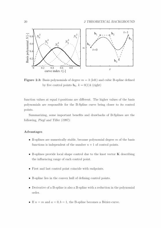
Figure 2.3: Basis polynomials of degree m = 3 (left) and cubic B-spline defined
by five control points bk, k = 0(1)4 (right)
function values at equal t-positions are different. The higher values of the basis
polynomials are responsible for the B-Spline curve being closer to its control
points.
Summarizing, some important benefits and drawbacks of B-Splines are the
following, Piegl and Tiller (1997):
Advantages
• B-splines are numerically stable, because polynomial degree m of the basis
functions is independent of the number n + 1 of control points.
• B-splines provide local shape control due to the knot vector K describing
the influencing range of each control point.
• First and last control point coincide with endpoints.
• B-spline lies in the convex hull of defining control points.
• Derivative of a B-spline is also a B-spline with a reduction in the polynomial
order.
• If n = m and a = 0, b = 1, the B-spline becomes a Bezier-curve.

2.3 NUMERICAL OPTIMIZATION 21
Disadvantage
• Time consuming determination of the piecewise defined basis functions
based on recursive scheme.
In terms of curve parameterization, cubic B-splines with a uniform knot vector
K should be the first choice, Farin (2000). They are a good compromise between
curve smoothness (C2 continuity, i.e. continuous in first and second derivatives)
and computational cost for determination of the cubic basis polynomials, Harries
(1998). In general, the design freedom can be varied by adding or subtracting
further control points which makes them more flexible and suitable for various
applications.
2.3 Numerical Optimization
In the last century, optimization has become more and more popular. Optimiza-
tion is used within various disciplines and for miscellaneous purposes. Airlines
are using mathematical optimization extensively in order to optimize the sched-
ule of the pilots, the flight attendants, and the flight plan itself. In the field of
transportation optimization solves logistical problems where the goal is to mini-
mize the time or the costs for transporting freight or passengers from one point to
another. Companies are optimizing their products in terms of quality, reliability,
costs, and efficiency.
The enormous development in the field of computer technology and the im-
provements of numerical algorithms in the last decades are responsible for the
growing acceptance of numerical optimization. In order to use optimization prop-
erly, first the optimization problem has to be analyzed and the design goals have
to be identified. They can be profit, time, efficiency, loss, or any other quantity
or combination of quantities that can be evaluated by a number. Unknown goals
are often used as objectives which have to be minimized or maximized whereas
known goals or restrictions are typically treated as equality or inequality con-
straints during the optimization process.
The objectives, and sometimes the constraints as well, are functions which
depend on certain parameters, called design variables or parameters that are to be
modified. The purpose of optimization is to find optimal values for these design

22 2 THEORETICAL BACKGROUND
parameters which minimize or maximize the objective function values. Often
design variables or any other parameters have to be restricted or constrained in
some way in order to guarantee feasible solutions, e.g. quantities such as mass or
length have to be positive.
The process of identifying objectives, design variables and constraints for a
given problem is probably the most important step in setting up the optimization
problem. If constraints are ignored or bounds on design parameters are made
poorly, optimization will not provide useful insight into the problem. On the
other side, if parameters are too restricted, optimization will find only sub-optimal
solutions or in the worst case it may become too difficult to solve the optimization
problem at all.
Another important point is a proper choice of the optimization algorithm. It
depends significantly on the properties of the optimization problem to be solved.
Hence, a classification of the optimization problem is extremely useful from the
computational point of view since there are many special methods available for
solving these particular classes of problems efficiently, Rao (1996). Depending
on whether or not constraints exist in the problem, any optimization task can
be classified as constrained or unconstrained problem. A further classification
can be done based on the mathematical expressions for the objective function
and the constraints. According to this, the optimization problem could be dis-
tinguished between linear, nonlinear, and quadratic programming problems. An
essential question is, however, the number of objective functions involved in the
optimization problem. This leads to the point where single- and multi-objective
optimization problems have to be distinguished.
2.3.1 Single-Objective Optimization
If the optimization task consists of one objective only, the design problem is called
mono- or single-objective problem. Mathematically speaking, single-objective
optimization is the minimization or maximization of an objective function f de-
pending on its design variables summarized in the design vector p subject to K
equality constraints h, J inequality constraints g and bounds on the design para-
meters or the objective function itself. The optimization problem can be written
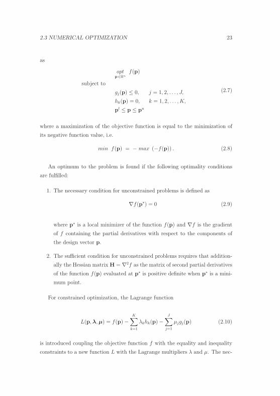
2.3 NUMERICAL OPTIMIZATION 23
as
optp∈Rn
f(p)
subject to
gj(p) ≤ 0, j = 1, 2, . . . , J,
hk(p) = 0, k = 1, 2, . . . , K,
pl ≤ p ≤ pu
(2.7)
where a maximization of the objective function is equal to the minimization of
its negative function value, i.e.
min f(p) = − max (−f(p)) . (2.8)
An optimum to the problem is found if the following optimality conditions
are fulfilled:
1. The necessary condition for unconstrained problems is defined as
∇f(p∗) = 0 (2.9)
where p∗ is a local minimizer of the function f(p) and ∇f is the gradient
of f containing the partial derivatives with respect to the components of
the design vector p.
2. The sufficient condition for unconstrained problems requires that addition-
ally the Hessian matrix H = ∇2f as the matrix of second partial derivatives
of the function f(p) evaluated at p∗ is positive definite when p∗ is a mini-
mum point.
For constrained optimization, the Lagrange function
L(p, λ, μ) = f(p) −K∑
k=1
λkhk(p) −J∑
j=1
μjgj(p) (2.10)
is introduced coupling the objective function f with the equality and inequality
constraints to a new function L with the Lagrange multipliers λ and μ. The nec-

24 2 THEORETICAL BACKGROUND
essary conditions for constrained optimization have been formulated by Karush
and Kuhn-Tucker, Fletcher (2000), and are defined as
∂f
∂p−
K∑k=1
λk∂hk
∂p−
J∑j=1
μj∂gj
∂p= 0, (2.11)
g(p) ≤ 0, (2.12)
h(p) = 0, (2.13)
μ ≤ 0, (2.14)
μjgj(p) = 0 (2.15)
or with the Lagrange function, Bestle (1994), as
∂L
∂p= 0,
∂L
∂λ= 0,
∂L
∂μ≥ 0, μ ≤ 0, μjgj(p) = 0. (2.16)
2.3.2 Multi-Objective Optimization
Most real-world design or decision problems are multi-objective or vector prob-
lems which involve simultaneous optimization of multiple objectives. Generally
speaking, the goal of a multi-objective optimization problem is to optimize the
design parameter vector p characterized by the minimization or maximization
of M objective functions f and associated equality and inequality constraints.
Mathematically the multi-objective optimization problem can be stated in its
general form as
optp∈Rn
f(p)
subject to
gj(p) ≤ 0, j = 1, 2, . . . , J,
hk(p) = 0, k = 1, 2, . . . , K,
pl ≤ p ≤ pu
(2.17)
Despite the fact that the mathematical formulation of the optimization prob-
lem looks quite similar to single-objective optimization, multi-objective optimiza-
tion is very different. Beside the design space in which each combination of design

2.3 NUMERICAL OPTIMIZATION 25
parameters is available a second space with the attainable objective function val-
ues exist. Figure 2.4 shows the mapping process of a design represented by the
design vector p as part of the feasible design space P to the attainable objective
space F of a bi-criterion design problem.
p2
design space
p
f2
f1
objective space
p1
f p( )
� �
Figure 2.4: Illustration of design space and objective space for a bi-criterion
design problem
As described in the previous Section 2.3.1, the aim of a single-objective optimiza-
tion is the attempt to obtain the best solution to the problem, which is usually
the global minimum or the maximum. In case of multiple objectives the contra-
diction between individual objectives leads to the problem that there may not
exist solely one solution which is best with respect to all objectives of the design
problem. In a typical multi-objective optimization problem there exists a set of
solutions which are superior to the rest of solutions in the search space when all
objectives are considered but are inferior to other solutions in the space in at least
one objective. Mathematically speaking, in multi-objective optimization a design
p1 is better than p2 in the case of minimization, if the corresponding objective
functions f1 := f(p1) and f2 := f(p2) are related as
f1 < f2, i.e. (f1i ≤ f2
i ∀ i ∈ M) ∧ (f1 �= f2), (2.18)
Bestle (1994). These solutions are known as non-dominated solutions or Pareto-
optimal solutions, where the rest of the solutions are called dominated solutions.
Figure 2.5 shows an example of an objective space for a bi-criterion minimiza-
tion problem with conflicting objectives f1 and f2. A sorting among the solutions

26 2 THEORETICAL BACKGROUND
A to E can be done using the principle of dominance. In this particular case,
solution D is dominated by solution A and B, while E is dominated by solution
C and B since they are better in both or at least in one objective without being
worse in the other. However, since none of the solutions in the non-dominated
set A-C is absolutely better than any other, i.e. better in both objectives, each
of them is an acceptable solution to the multi-objective minimization problem.
f2
f1
B
A
D
E
C
Figure 2.5: Principle of dominance for a bi-criterion minimization problem
In this particular case where both objectives are being minimized, the Pareto-
optimal solutions are located at the lower left border of the attainable objective
space. For a different combination of minimization and maximization of objec-
tives the Pareto-optimal front varies. In Figure 2.6 four possible borders for
two-objective optimization problems are indicated.
The benefit of multi-objective optimization compared to the classical single-
objective problem is to provide different solutions to the design problem from
which the engineer or designer can choose. The choice of one solution over the
other requires problem knowledge or additional decision criteria which are not
explicitly formulated in the design task. Thus, one solution selected by a designer
may not be acceptable to another designer. Therefore, it may be useful to have
knowledge about as much trade-offs as possible within Pareto-optimal solutions,
i.e. a wide set of non-dominated solutions from which one or more solutions can
be chosen after the optimization process according to some decision-makers.

2.3 NUMERICAL OPTIMIZATION 27
f2
a)
f1
f2
b)
f1
min-max max-max
f2
c)
f1
f2
d)
f1
min-min max-min
Figure 2.6: Location of the Pareto-optimal solutions for a bi-criterion optimiza-
tion problem: a) minimizing f1 and maximizing f2, b) maximizing
both objectives, c) minimizing both objectives, d) maximizing f1
and minimizing f2
Hence, in multi-objective optimization two goals are pursued simultaneously, Deb
(2001):
1. finding a set of solutions as close as possible to the Pareto-optimal front,
2. finding a set of solutions as diverse as possible.
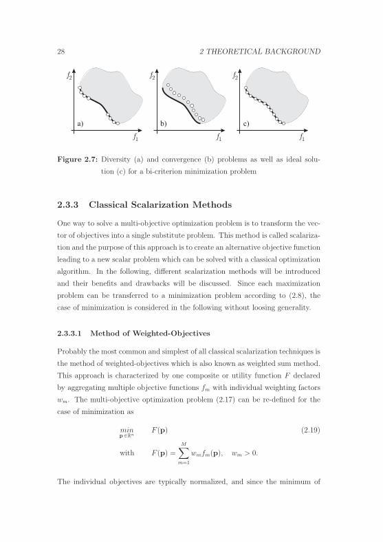
Figure 2.7 illustrates three different results for the same multi-objective opti-
mization problem. As can be seen for the first case, Figure 2.7a, the fairly good
solutions found by the optimizer are placed at the Pareto-front, however, a huge
gap between the solutions exists and the diversity is rather poor. The results
shown in Figure 2.7b are distributed more homogeneously, but the convergence
towards the Pareto-front is rather poor, and therefore these solutions would not
be acceptable. The ideal case is shown in Figure 2.7c, where all solutions are
located along the Pareto-front and are uniformly distributed.
28 2 THEORETICAL BACKGROUND
f2
f2
a) b)
f2
c)
f1
f1
f1
Figure 2.7: Diversity (a) and convergence (b) problems as well as ideal solu-
tion (c) for a bi-criterion minimization problem
2.3.3 Classical Scalarization Methods
One way to solve a multi-objective optimization problem is to transform the vec-
tor of objectives into a single substitute problem. This method is called scalariza-
tion and the purpose of this approach is to create an alternative objective function
leading to a new scalar problem which can be solved with a classical optimization
algorithm. In the following, different scalarization methods will be introduced
and their benefits and drawbacks will be discussed. Since each maximization
problem can be transferred to a minimization problem according to (2.8), the
case of minimization is considered in the following without loosing generality.
2.3.3.1 Method of Weighted-Objectives
Probably the most common and simplest of all classical scalarization techniques is
the method of weighted-objectives which is also known as weighted sum method.
This approach is characterized by one composite or utility function F declared
by aggregating multiple objective functions fm with individual weighting factors
wm. The multi-objective optimization problem (2.17) can be re-defined for the
case of minimization as
minp∈Rn
F (p) (2.19)
with F (p) =M∑
m=1
wmfm(p), wm > 0.
The individual objectives are typically normalized, and since the minimum of

2.3 NUMERICAL OPTIMIZATION 29
the above problem does not change if all weights are multiplied by a constant
value, it is usual practice to choose weights such that their sum is equal to one,∑Mm=1 wm = 1, Deb (2001).
The application of the weighted-objectives method on a bi-criterion minimiza-
tion problem is demonstrated in Figure 2.8. Since the composite function F is
a linear combination of the objectives f1 and f2, its contour lines are straight in
the objective space and the slope of the solution levels are defined by the ratio
−w1/w2 of the weighting factors, Figure 2.8a. The task of the minimization pro-
cedure is to find the minimum function value of F obtained by the contour line
which is tangential to the feasible solution space at the bottom-left corner. Hence,
Point A is a Pareto-optimal solution of the minimization problem corresponding
to the chosen weighting factors.
It is clear that the preference of an objective can be changed by modifying
the corresponding weighting factor which leads to another solution point. This
effect can be used in order to find the Pareto-front by obtaining different points
on the curve with different combinations of weighting factors, Figure 2.8b. A
sequential variation with small incrementing steps of some weighting factors can
be used to find as much trade-off solutions as possible. This technique works fine
for convex Pareto-fronts only, while for non-convex cases multiple solutions for
constant weighting factors could exist and not all points on the Pareto-front can
be determined, Figure 2.8c.
f2
w w1 2>
f1
b)w w
2 1>
f2
f1
c)
A
B
A
B
f1
a)
A
w2
-w1
f2
�
fF
Figure 2.8: Illustration of the method of weighted-objectives: a) contour lines
of composite function, b) results for different weighting factors for a
convex Pareto-front, c) multiple solutions for a non-convex Pareto-
front while solutions in between A and B cannot be determined
30 2 THEORETICAL BACKGROUND
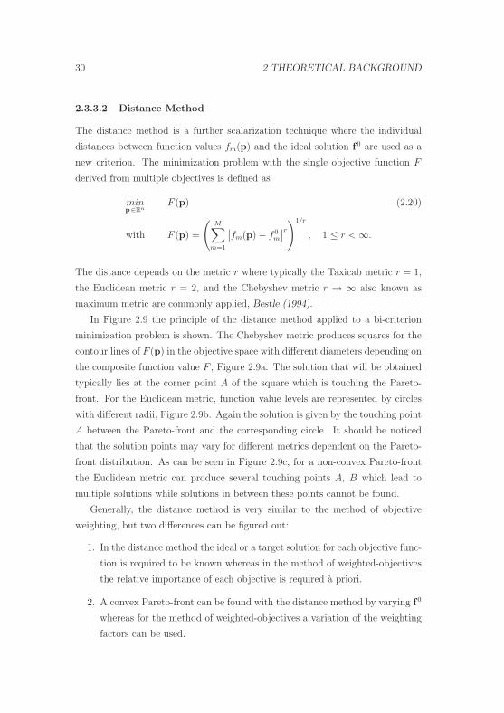
2.3.3.2 Distance Method
The distance method is a further scalarization technique where the individual
distances between function values fm(p) and the ideal solution f0 are used as a
new criterion. The minimization problem with the single objective function F
derived from multiple objectives is defined as
minp∈Rn
F (p) (2.20)
with F (p) =
(M∑
m=1
∣∣fm(p) − f 0m
∣∣r)1/r
, 1 ≤ r < ∞.
The distance depends on the metric r where typically the Taxicab metric r = 1,
the Euclidean metric r = 2, and the Chebyshev metric r → ∞ also known as
maximum metric are commonly applied, Bestle (1994).
In Figure 2.9 the principle of the distance method applied to a bi-criterion
minimization problem is shown. The Chebyshev metric produces squares for the
contour lines of F (p) in the objective space with different diameters depending on
the composite function value F , Figure 2.9a. The solution that will be obtained
typically lies at the corner point A of the square which is touching the Pareto-
front. For the Euclidean metric, function value levels are represented by circles
with different radii, Figure 2.9b. Again the solution is given by the touching point
A between the Pareto-front and the corresponding circle. It should be noticed
that the solution points may vary for different metrics dependent on the Pareto-
front distribution. As can be seen in Figure 2.9c, for a non-convex Pareto-front
the Euclidean metric can produce several touching points A, B which lead to
multiple solutions while solutions in between these points cannot be found.
Generally, the distance method is very similar to the method of objective
weighting, but two differences can be figured out:
1. In the distance method the ideal or a target solution for each objective func-
tion is required to be known whereas in the method of weighted-objectives
the relative importance of each objective is required a priori.
2. A convex Pareto-front can be found with the distance method by varying f0
whereas for the method of weighted-objectives a variation of the weighting
factors can be used.

2.3 NUMERICAL OPTIMIZATION 31
f2
f1
a)
f2
f1
c)
A
f1
0
f2
0
rA
r = 2
B
f1
b)
A
f2
f2
0
r = 2
�
fF
�
fF
�
fF
f1
0f1
0
f2
0
Figure 2.9: Principle of distance method for a bi-criterion minimization prob-
lem: a) Chebyshev metric at convex Pareto-front, b) Euclidean
metric at convex Pareto-front, c) Euclidean metric at non-convex
Pareto-front
2.3.3.3 Compromise Method
The idea of the compromise method, which is also named ε-constraint method,
is that only one of the original objectives is being optimized whereas the others
are taken into account as inequality constraints during the optimization process.
The multi-objective minimization problem for a freely chosen objective fr(p),
r ∈ [1, . . . , M ] and upper bounds fj for the M − 1 remaining criteria fj can be
re-written as
minp∈Rn
fr(p)
subject to
fj(p) ≤ fj, j �= r.
(2.21)
The compromise method is very useful and can give a good insight to the
optimization problem. By relaxing the bounds for the constraints, a further min-
imization of the objective function is possible whereas more restricted constraints
are increasing the objective function value, respectively. An iterative process with
sequentially relaxing or restricting the bounds can be used to find additional solu-
tions on the Pareto-front. In order to resolve the whole Pareto-curve, very small
step-sizes for the bounds have to be chosen. It is interesting to know that on the
one hand this method works for convex as well as for some non-convex solution
spaces depending on their complexity, Deb (2001), and on the other hand that
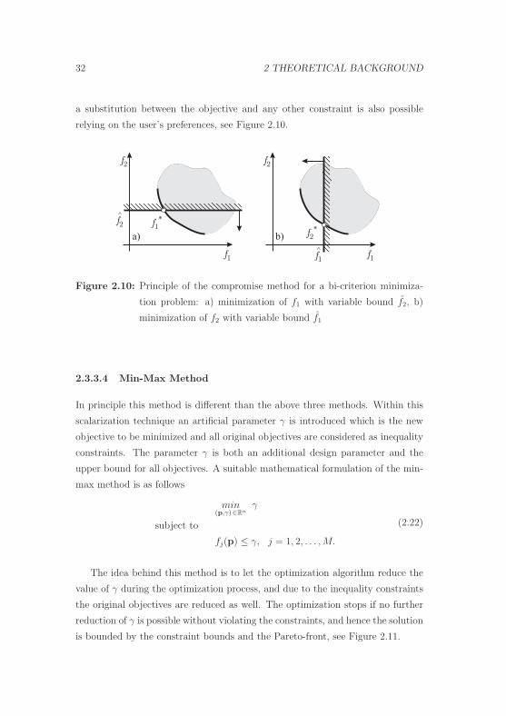
32 2 THEORETICAL BACKGROUND
a substitution between the objective and any other constraint is also possible
relying on the user’s preferences, see Figure 2.10.
f2
f1
a)
f1
*f2
^
f2
f1
b) f2
*
f1
^
Figure 2.10: Principle of the compromise method for a bi-criterion minimiza-
tion problem: a) minimization of f1 with variable bound f2, b)
minimization of f2 with variable bound f1
2.3.3.4 Min-Max Method
In principle this method is different than the above three methods. Within this
scalarization technique an artificial parameter γ is introduced which is the new
objective to be minimized and all original objectives are considered as inequality
constraints. The parameter γ is both an additional design parameter and the
upper bound for all objectives. A suitable mathematical formulation of the min-
max method is as follows
min(p,γ)∈Rn
γ
subject to
fj(p) ≤ γ, j = 1, 2, . . . , M.
(2.22)
The idea behind this method is to let the optimization algorithm reduce the
value of γ during the optimization process, and due to the inequality constraints
the original objectives are reduced as well. The optimization stops if no further
reduction of γ is possible without violating the constraints, and hence the solution
is bounded by the constraint bounds and the Pareto-front, see Figure 2.11.

2.3 NUMERICAL OPTIMIZATION 33
f2
f1
a)
f(p ),�
f1
f(p ),�
f1
f(p ),�
f2
b)
f2
c)
� ��
�
�
�
Figure 2.11: Progress of min-max optimization for a bi-criterion minimization
problem: a) loose bounds as optimization starts, b) more re-
stricted bounds during optimization, c) final bounds and solution
at Pareto-front
2.3.3.5 Discussion about Scalarization Methods
In all of the above mentioned scalarization methods, multiple objectives are com-
bined to form one objective by using some knowledge on the problem being solved.
The optimization of the single-objective may guarantee a Pareto-optimal solution
for a convex Pareto-front, but results in a single solution point only.
In real-world technical problems, engineers often need different alternatives or
trade-offs for decision making. Moreover, if some of the objectives are noisy, have
discontinuous variable space, or the Pareto-optimal solution front is non-convex,
these methods may not work effectively. The most profound drawbacks of these
methods are that
1. they require knowledge of individual optima or the attainable objective
space at all prior to starting the optimization,
2. solutions obtained largely depend on the method settings, e.g. underlying
weight-vector for the method of weighted-objectives, the chosen metric for
distance method, and the step sizes for compromise method,
3. the same problem needs to be solved a number of times with variable pa-
rameter settings in order to find as much points on the Pareto-front as
possible.
Nevertheless, using scalarization methods is sometimes a good choice if a quick

34 2 THEORETICAL BACKGROUND
single solution to the problem is required or a classical single-objective optimiza-
tion method is available only. It is always the user’s responsibility to choose a
proper method and proper settings according to the problem definition.
2.3.4 Optimization Algorithms
Once objective, design parameters, and constraints are formulated an optimiza-
tion algorithm must be chosen for solving the problem. There is no universal
optimization algorithm, rather there are numerous algorithms available which
are tailored to particular types of optimization problems. The choice of an ap-
propriate algorithm is an important one; it determines whether the problem is
solved rapidly or slowly and, indeed, whether the solution is found at all.
Figure 2.12 shows a simple minimization problem with a smooth and contin-
uous function depending on a single variable. In spite of its simplicity, different
extrem values for the non-convex objective function f exist, and in terms of
numerical optimization, finding the best solution to this particular multi-modal
problem is not as trivial as it seems to be. Indeed, various optimization algorithms
will behave in a different manner and the right choice of the optimization method
is rather important for finding the optimum. Algorithms which are searching
based on descend directions would typically find the next local minimum to the
starting point which is not necessarily the global minimum, whereas global opti-
mization algorithms have a strategy based on a stochastic approach which makes
them able to find the global minimum to the problem.
In the last decades a tremendous number of publications has been pub-
lished presenting new optimization algorithms, variants of existing methods
as well as hybrid methods which combine two or more algorithms. In some
classical text books, Bestle (1994), Coello Coello et al. (2002), Fletcher (2000),
Gill et al. (1995), Rao (1996), More and Wright (1994), classifications and de-
scriptions of optimization algorithms are available which give an overview of
existing methods, and which can basically help choosing the right algorithm for
a specific type of optimization problem. In the following section one of these
classifications will be discussed in more detail.

2.3 NUMERICAL OPTIMIZATION 35
global minimum
local minimum
f
f ( )p
p
local minimum
Figure 2.12: Illustration of global and local minima for a simple one-
dimensional function
2.3.4.1 Classification of Optimization Algorithms
One possible method of classifying optimization algorithms can be derived from
their working principles. An optimization procedure starts typically from an
initial design characterized by the design vector p(1). During optimization a
series of designs are created which decrease the objective function value (for the
case of minimization) step by step, i.e. f(p(k+1)) < f(p(k)). The general form of
this series is given by
p(k+1) = p(k) + α(k)d(k), (2.23)
with the step size α(k) ≥ 0 and the search direction d(k). In general, optimization
algorithms differ in how they determine the next design vector p(k+1). They can be
globally distinguished as deterministic or stochastic algorithms, see Figure 2.13.

36 2 THEORETICAL BACKGROUND
Gradient BasedMethods
Derivative-FreeMethods
StochasticMethods
Optimization Algorithms
DeterministicMethods
EvolutionaryAlgorithms
SimulatedAnnealing
Figure 2.13: Classification of optimization algorithms
2.3.4.2 Deterministic Algorithms
Deterministic algorithms search according to clearly defined rules based on alge-
braic or analytical schemes. The optimization procedure can be described by the
following steps:
1. Start with a given design vector p(k) and evaluate its corresponding function
value f(p(k)).
2. Determine a search direction d(k).
3. Solve a one-dimensional line search problem in order to find the right step
size α(k).
4. Calculate the new design vector by p(k+1) = p(k) + α(k)d(k) and its function
value f(p(k+1)).
5. Repeat steps 2-4 with the new design point until convergence is achieved.
Most deterministic algorithms are working based on this concept. The dif-
ferences between the individual methods rely on the determination of the search
direction and on the line search procedure. In the past, much effort was un-
dertaken for a precise determination of the step size α(k), where the line search
procedure has been formulated as an independent minimization task within the
optimization step. This time-consuming process is not required in today’s al-
gorithms where typically the line search is performed on simple techniques as

2.3 NUMERICAL OPTIMIZATION 37
the Armijo-rule, the golden section method and sometimes on spline or parabola
approximation models, Bestle (1994). It has been shown that a better determi-
nation of the search direction is more important than the line search in terms of
higher convergence rates and better solution finding. Therefore, it is better to
distinguish the different algorithms based on their search direction determination.
In general, deterministic algorithms can be subdivided into gradient based
methods which compute the search direction on the basis of calculated or ap-
proximated gradients and sometimes even on curvature information, and the more
simple search methods or derivative-free methods which determine the search di-
rection by evaluating function values only.
Derivative-Free Methods
The most common derivative-free methods are the Pattern-Search-Methods,
Lewis et al. (2000), the Simplex-Method developed by Nelder and Mead (1965),
the Hooke-Jeeves-Method, Hooke and Jeeves (1961), and the Conjugate-
Directions-Method, Fletcher and Reeves (1964). Their advantage in comparison
with other methods is that they are not requiring any gradient or curvature infor-
mation. Their search algorithm is based on evaluation of the objective function
value only while in some cases even the actual numeric value of the objective func-
tion is unimportant, but it is sufficient to know whether a design is better than
another or not, Birk (2003). This makes them suitable for optimization problems
with expensive and noisy objective functions where an approximation of the gra-
dients is too costly or too inaccurate. These search methods were used in the past
and are still used for solving specific types of real-world optimization problems.
Today, however, these methods are not the best choice for solving engineering
applications which are characterized by a huge number of design variables and
constraints, and where the entire optimization time for solving the design task
plays an essential role.
Gradient Based Methods
Better approaches in terms of optimization time are the more sophisticated gradi-
ent based methods which are superior to derivative-free methods to some extent.
They are used to solve a whole bunch of engineering design problems due to their
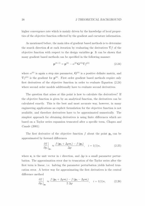
38 2 THEORETICAL BACKGROUND
higher convergence rate which is mainly driven by the knowledge of local proper-
ties of the objective function reflected by the gradient and curvature information.
As mentioned before, the main idea of gradient based methods is to determine
the search direction d at each iteration by evaluating the derivatives ∇f of the
objective function with respect to the design variables p. It can be shown that
many gradient based methods can be specified in the following manner:
p(k+1) = p(k) − α(k)G(k)∇f (k) (2.24)
where α(k) is again a step size parameter, G(k) is a positive definite matrix, and
∇f (k) is the gradient for p(k). First order gradient based methods require only
first derivatives of the objective function in order to evaluate Equation (2.24)
where second order models additionally have to evaluate second derivatives.
The question that arises at this point is how to calculate the derivatives? If
the objective function is given by an analytical function, the derivatives can be
calculated exactly. This is the best and most accurate way, however, in many
engineering applications an explicit formulation for the objective function is not
available, and therefore derivatives have to be approximated numerically. The
simplest approach for obtaining derivatives is using finite differences which are
based on a Taylor series expansion truncated after a specific term, Chapra and
Canale (2001).
The first derivative of the objective function f about the point p0 can be
approximated by forward differences
∂f
∂pi
∣∣∣∣p0
≈ f (p0 + Δp ei) − f (p0)
Δp, i = 1(1)n, (2.25)
where ei is the unit vector in i direction, and Δp is a small parameter pertur-
bation. The approximation error due to truncation of the Taylor series after the
first term is linear, i.e. halving the parameter perturbation yields halved trun-
cation error. A better way for approximating the first derivatives is the central
difference method
∂f
∂pi
∣∣∣∣p0
≈ f (p0 + Δp ei) − f (p0 − Δp ei)
2 Δp, i = 1(1)n, (2.26)

2.3 NUMERICAL OPTIMIZATION 39
which is more accurate. In contrast to the forward difference approximation the
truncation error here would be quartered for halving the perturbation.
Applied to an optimization problem the number of function evaluations in-
creases significantly with the number of design parameters. For a full determina-
tion of the gradient ∇f by using forward differences, n + 1 function evaluations
are necessary for a n-dimensional design problem, and for the more accurate cen-
tral differences 2n+1 calculations are required at each optimization step. Besides
this, it is essential that the objective function exists for all perturbed designs, i.e.
that e.g. iterative computations converge and yield results, the objective is not
too noisy, and the parameter perturbation is chosen appropriately.
A further important point to consider is that in gradient based methods the
objective function as well as constraints are assumed to be smooth which means
that they are twice continuously differentiable. The problem in most engineering
applications, however, is that this property is often a priori unknown, but nev-
ertheless it is common practice to assume smoothness and to check later if the
algorithm converges properly and produces reasonable results.
At this point some of the most common gradient based algorithms should be
discussed. A more detailed overview of existing algorithms and comparisons with
other methods can be found in classical text books like Gill et al. (1995) and
Fletcher (2000).
Probably one of the best known first order gradient based algorithms is the
method of Steepest Descent in which it is assumed that the best search direction
is where the objective function value decreases most rapidly. This is given by
the negative gradient at each step k, i.e. d(k) = −∇f (k). If the positive definite
matrix G(k) is set equal to the identity matrix I, Equation (2.24) with the step
size α(k) becomes
p(k+1) = p(k) − α(k)∇f (k). (2.27)
Despite their linear convergence property these type of methods usually exhibit a
quick convergence at the beginning which then leads to oscillatory or zig-zagging
behavior, and usually the algorithms terminate far from the solution owing to
round-off effects. Therefore in practice they are inefficient and unreliable, Fletcher
(2000).

40 2 THEORETICAL BACKGROUND
More powerful are the Newton or Newton-Raphson type second order gradient
based methods which are based on the gradient as well as on curvature informa-
tion. Within these methods, the positive definite matrix G(k) is set equal to the
inverse Hessian matrix H(k)−1, with H(k) = ∇2f (k), and the next design point is
determined by
p(k+1) = p(k) − α(k)H(k)−1∇f (k). (2.28)
The benefit of these second order algorithms is that they show quadratic con-
vergence, and hence they are the fastest known methods. In contrast to the
Steepest Descent Methods, the computational costs for the Hessian matrix is a
major drawback of these algorithms and, especially if the second order derivatives
are also approximated by finite differences, the computational time for evaluating
the objective function f increases extremely, Birk (2003).
A good compromise between the first and second order gradient based meth-
ods are the Quasi-Newton Methods which are characterized by a good conver-
gence rate and relatively low computational costs for the search direction. The
idea behind these types of methods is to avoid the expensive determination of
the exact Hessian matrix at every step either by calculating the Hessian only
every few steps or by approximating the Hessian or its inverse by a symmetric
positive definite matrix B. In the latter approach, the matrix B is initially set
equal to the identity matrix I and while the optimization proceeds it is corrected
or updated from iteration to iteration using an appropriate update scheme. The
key point is that most update schemes are using the information of first deriva-
tives only which has positive influence on the overall computational time. The
Davidon-Fletcher-Powell (DFP) and Broyden-Fletcher-Goldfarb-Shanno (BFGS)
update schemes should be mentioned at this point as common methods within
numerous algorithms, Fletcher (2000).
The gradient based algorithms described up to this point are basically de-
veloped for unconstrained optimization problems. However, some methods exist
to use them also if constraints are introduced. One possibility is by replacing
the constrained optimization problem with an unconstrained one by adding a
penalty function to the objective function that depends on the value of the vio-
lated constraints. This method is called Penalty-Method and depending on the

2.3 NUMERICAL OPTIMIZATION 41
formulation of the penalty function, it can be distinguished between interior and
exterior Penalty-Methods. In general, these methods provide an easy way to con-
sider constraints in an optimization problem which makes them suffice for special
purposes. Nevertheless, some major drawbacks exist why they are not suitable
for general applications, Bestle (1994).
The current state of the art for solving constrained optimization problems
with gradient based methods are the Lagrange-Newton type methods which are
also known as Sequential Quadratic Programming (SQP) algorithms due to their
mathematical background. The basic idea of these algorithms is to find an op-
timal search direction d(k) by solving a quadratic subproblem considering linear
constraints in each iteration. Compared to a simple search method, the determi-
nation of the search direction based on solving quadratic subproblems requires
significantly more computational effort. However, these methods show a very
quick convergence and are highly efficient in solving engineering optimization
problems, Birk (2003).
2.3.4.3 Stochastic Algorithms
The idea of stochastic algorithms is generally different compared to deterministic
methods. They use a stochastic approach in order to find a better design in-
stead of any gradient information. This property makes them capable to find a
global optimum to the design problem and not to be trapped in a local optimal
solution. Since the determination of the next design parameters is usually not
pure random, these types of algorithms are also called semi-stochastic or heuris-
tic algorithms. Their benefit compared to gradient based methods is basically
that they are able to cope with a wide range of features in optimization problems
like discrete and continuous design variables, noisy or discontinuous objective
functions, and multi-modal problems. However, Stochastic Algorithms are also
considered to be computationally expensive in terms of the required number of
evaluated solutions for convergence, Buche (2004). In the following, Simulated
Annealing and Evolutionary Algorithms as two well known representations of
stochastic algorithms will be discussed.

42 2 THEORETICAL BACKGROUND
Simulated Annealing
Simulated Annealing methods are stochastic algorithms which mimic the recrys-
tallization of a liquid metal during annealing. Heated up to high temperatures,
the atomic structure becomes disordered which makes the atoms capable of mov-
ing around in the melt. The melt is kept near its thermodynamic equilibrium
when it is slowly cooled down. This drives the individual atoms to reach the
minimum energy state and the nearly perfect crystalline structure is formed, i.e.
the global minimum is found. The initial situation as well as the cooling process
itself are important factors within the annealing procedure. If the initial tem-
perature is too low or the cooling process too fast, the structure becomes frozen
before it reaches the desired minimum energy state and a local minimum to the
problem is found, Birk (2003).
Transferred to an arbitrary engineering optimization problem, Simulated An-
nealing methods try to find the global optimum to the design problem by a
sequence of numerical steps. The algorithm starts with an initial temperature
T (k=0) and an initial design point which in the beginning is also the best known
solution p∗ ≡ p(k=0). A new design is created randomly in the neighborhood of
the best point while the random disturbance is larger for higher temperatures.
The function value of the new design is compared with the best solution and if it
is better, i.e. Δ = f(p(k+1))−f(p∗) < 0, then this is taken as new best design and
the next iteration can start with a lower temperature T (k+1) < T (k) resulting in a
smaller random disturbance. Otherwise the new design is accepted as best design
only with a lower probability depending on the temperature. The algorithm pro-
ceeds until the minimum temperature level is found, Kirkpatrick et al. (1983). In
contrast to deterministic optimization algorithms, new designs with higher func-
tion values are accepted with some probability which is the reason why Simulated
Annealing is able to leave already established local minima to reach the global
minimum.
Evolutionary Algorithms
Another group of stochastic methods are called Evolutionary Algorithms. In gen-
eral these algorithms are inspired by the principles of natural evolution to find
an optimal solution to a problem. Natural evolution is driven by the principles

2.3 NUMERICAL OPTIMIZATION 43
of selection, recombination and mutation of genetic information. Individuals in a
population which are well adapted to their environment have a higher probability
to survive in the nature, known as ’survival of the fittest’. These individuals are
declared with a higher fitness value and are chosen in order to become parents
(selection) which produce offsprings for the following generation. The genetic
information of the offspring is either a direct copy of the genes of just one sin-
gle parent, which differs from the natural evolution, or results from the mating
process of multiple parents (recombination or crossover). In the latter case the
gene of the offspring is arranged form gene sequences of both parents. Addition-
ally, a randomly generated mutation can modify the genetic information of the
offsprings (mutation) and the best solutions are selected in the selection process.
Figure 2.14 shows the principle work flow of an evolutionary algorithm consisting
of crossover, mutation, and selection.
Mutation
Selection
Converged?
Crossover
NewPopulation
StartOptimization
FinishOptimization
yes
no
Figure 2.14: Principle work flow of an evolutionary algorithm
Applied to engineering design problems, the genetic information corresponds
to the design variables which specify the properties of a solution to the engineering
optimization problem, and the fitness of a solution is either determined directly
by the objective function or by a combination between the objective function
value and the constraints.
It should be mentioned that Evolutionary Algorithms (EA) are building an up-
per class of algorithms containing the subgroups of Genetic Programming (GP),
Genetic Algorithms (GA), and Evolutionary Strategies (ES), Back et al. (1997).
Genetic Algorithms were firstly proposed and applied by Holland (1975) while
Rechenberg (1973) developed Evolutionary Strategies independently and applied

44 2 THEORETICAL BACKGROUND
them to some engineering design problems. Although based on a similar idea,
both approaches were different in some aspects at the beginning of their devel-
opment. In Genetic Algorithms an individual is represented by a string of bits
and the evolutionary process is based on selection, recombination, and mutation
techniques. In contrast to this, in Evolutionary Strategies each individual of the
population is represented by a vector of real design variables and the evolution-
ary process is characterized by selection and mutation techniques only. However,
nowadays modern algorithms are mixed up with both ideas and hence it is often
not simple to classify them anymore.
2.3.4.4 Algorithms Used in this Thesis
Since all of the described strategies have their strengths and weaknesses, different
types of algorithms have been chosen to solve the optimization problems within
this thesis. Especially for complex design problems like aerodynamic compressor
design it is not a priori known which method will work best. Thus, one goal of
the thesis is to gather experience in the behavior of different strategies on the
various subtasks. The selected optimization algorithms are as follows:
Lagrange-Newton Method NLPQL
The Nonlinear Programming with Quadratic Line Search algorithm (NLPQL)
was developed by Schittkowski (1986). It is a Lagrange-Newton type algorithm
for solving smooth, nonlinear, constrained optimization problems, i.e. minimiz-
ing a nonlinear objective function subject to nonlinear equality and inequality
constraints. It is assumed that all model functions are continuously differen-
tiable. The internal algorithm is a SQP method with a quadratic approximation
of the Lagrange function and a linearization of the constraints. Each iteration
step starts with a determination of the search direction by solving a quadratic
programming subproblem with an approximation of the Hessian matrix using
the BFGS update scheme and a subsequent line search which is performed for
determination of the step length α, Schittkowski (1981).

2.3 NUMERICAL OPTIMIZATION 45
Single-Objective Stochastic Method MIGA
When genetic algorithms are applied to an engineering design application, they
require many generations and a large number of individuals in the population in
order to obtain good solutions. The idea of the Multi-Island Genetic Algorithm
(MIGA), Miki et al. (2000a), which is a single-objective optimization algorithm,
is to accelerate the solution finding process by dividing the large population into
smaller sub-populations like on islands and to execute traditional genetic opera-
tions on each sub-population separately. The algorithm then periodically selects
individuals from each sub-population and moves them to other sub-populations in
an exchange called migration. Two parameters are basically driving the migration
process: the migration interval which is the number of generations between each
migration process, and the migration rate which is the percentage of individuals
selected for migration from each sub-population at the time migration occurs.
The emigrants are selected randomly in their sub-populations and the migration
topology is typically selected as a ring with random destinations where each sub-
population has one destination and the destinations are determined randomly at
every migration period, Kaneko et al. (2000).
In general it can be shown that genetic algorithms with a distributed popu-
lation show better performance in terms of convergence and fitness values than a
single population GA. Furthermore, this approach is suitable to be implemented
on parallel computers, because the communication between the processors occurs
only in the migration phase. Therefore, if each sub-population is assigned to
one processor of a parallel computer, a nearly linear reduction in speed can be
expected, Miki et al. (2000b).
Multi-Objective Stochastic Method NSGA-II
The Non-dominated Sorting Genetic Algorithm II (NSGA-II) is a multi-objective
genetic algorithm developed by Deb et al. (2000) and is a revised version of
NSGA, Srinivas and Deb (1995). In most aspects, the algorithm does not have
much similarity with the original NSGA, but the authors kept the name NSGA-II
to highlight its genesis and place of origin.
Figure 2.15 shows the basic idea of the algorithm. In NSGA-II the offspring
population Qt which is created by the parents and the parent population Pt

46 2 THEORETICAL BACKGROUND
itself are combined together to form an overall population Rt. A non-dominated
sorting algorithm based on the vector criterion of each individual is performed
on Rt. The new population Pt+1 is filled by solutions of different non-dominated
fronts Fi starting with the best non-dominated front F1 and continuing with
the next ones until the generation size is maintained. It may happen that the
number of individuals in the last considered solution front is bigger than the
available slot size. Instead of arbitrarily discarding some members from the last
front, a crowding algorithm is performed which estimates the distance of these
solutions to each other. The solutions of the last front with the highest diversity,
i.e. widely spread in the objective space, are included in the new population
Pt+1 whereby the rest of them are rejected. The next offsprings Qt+1 are created
based on the new population Pt+1 by tournament selection, recombination and
mutation operators, Deb (2001).
Pt
Qt
Rt
non-dominatedsorting
crowding distancesorting
rejected
Pt+1
F1
F2
F3
Figure 2.15: Illustration of the NSGA-II procedure, Deb (2001)
The NSGA-II is currently one of the most popular multi-objective genetic al-
gorithms. It basically consists of two major aspects: an elite-preserving operation
and a crowding algorithm. The non-dominated sorting algorithm carries over the
best solutions denoted as the elite of a generation to the next generation. Hence,
the fitness and the corresponding values of the objective functions of the best
solutions do not deteriorate and furthermore the best solutions found early in the
optimization process will never be lost unless a better solution is discovered. The
crowding algorithm is important to drive the required diversity of non-dominated
solutions and to distribute the solutions on the Pareto-front. Both aspects to-
gether makes the NSGA-II robust, reliable and applicable to many engineering
design problems.

3 Optimization Based
Preliminary Design
The aerodynamic compressor design process starts with the preliminary design
phase, where new design ideas or philosophies are investigated in terms of fea-
sibility and improvement. The calculation results, which are generally based on
analytical equations, give a rough overview on performance and stability criteria
that can be achieved for a specific compressor design. The calculation time is
rather short, however, a complete investigation of different design studies is man-
ually too expensive due to the huge number of design parameters and constraints.
On the basis of a given Rolls-Royce preliminary design tool, process integra-
tion and automation is applied in order to accelerate the meanline prediction
process and to support the design engineer in time-consuming parameter studies.
Numerical optimization is performed with the MIGA, NLPQL, and NSGA-II al-
gorithms to improve a given design of a 9-stage high pressure research compressor,
Klinger (2004), with respect to conflicting design goals as efficiency, surge margin
and overall pressure ratio. Based on design conditions, design changes are made
with respect to the annulus geometry and the stage pressure ratio distribution.
3.1 Introduction
Meanline prediction is the first step of the complex aerodynamic compressor de-
sign process. The goal is to provide a robust and reliable instrument for a first
guess and proper choice of design parameters for design and off-design condi-
tions. The performance that can be achieved by a well-designed multi-stage axial
47
48 3 OPTIMIZATION BASED PRELIMINARY DESIGN
compressor is mainly determined by the choices made for a number of global
parameters. No amount of subsequent development effort can correct a poor de-
sign where the basic selection of global parameters is inconsistent with the design
objectives. On account of this, meanline prediction as a preliminary design pro-
cedure setting the values of these global parameters is one of the very essential
steps of the entire aerodynamic compressor design process, Keskin and Bestle
(2005).
Within the preliminary design phase, calculations are performed along the
mid-height line of the compressor and the main aerodynamic and geometric pa-
rameters are determined, Figure 3.1. The process typically starts based on an
old initial axial compressor design and new performance requirements. Operating
conditions and geometric constraints in term of minimum or maximum radii of
the annulus or even sometime the maximum compressor length are a priori given
or restricted and have to be adjusted or adapted to the new design problem. Ba-
sically, the goal is to find appropriate design parameter distributions along the
one-dimensional mid-height streamline of the compressor which fulfill the design
requirements and constraints as good as possible.
The entire suite of available parameters describing the whole compressor
model can be split into design variables which are assumed to be adjustable
within the design process in order to fulfill design requirements, and system con-
stants which are invariant during the design calculation. The selection of the
design variables and the system constants depends on the design goals, the sensi-
tivities of the objective functions on parameter variations, and obviously on the
knowledge and expertise of the design engineer.
If a manual search for a good design is performed, only few parameters are
taken into account and small variations on the design variables are applied. Ob-
viously, it is too complicated for a human design engineer to understand the
dependence of the outputs on the inputs and if a large number of design pa-
rameters are changed simultaneously and many criteria and constraints have to
be considered. This manual search technique is rather time-consuming and the
success depends significantly on the experience of the engineer.
Therefore, it should be the overall aim to implement the preliminary design
process into a common design environment and to accelerate the design process
by automation of the engineering work flow. Due to the rather complex design

3.2 DESIGN PROBLEM 49
process with a huge number of design parameters and a high number of design
criteria for design and off-design conditions, it is more realistic at present to im-
prove the design process by partial automation of a specific work flow. When the
design process runs automated and the design parameters, objectives, and con-
straints are defined properly, numerical optimization can be applied to support
the design engineer in solution finding and decision making. Especially if conflict-
ing criteria exist, multi-objective optimization methods can find Pareto-optimal
trade-offs from which the design engineer can choose one or more solutions for
the particular design problem afterwards.
3.2 Design Problem
As already mentioned, many different design goals and a huge number of con-
straints have to be pursued in parallel in order to achieve a good preliminary
aerodynamic compressor design. It depends on the problem formulation if pa-
rameters as the compressor length, the number of stages, the overall pressure
ratio, and many more have to be considered as constraints or as objectives to
be optimized in this design task. The most important aerodynamic parameters,
however, are the efficiency and the stability of the compressor reflected by the
surge margin value which always have to be maximized at reasonable pressure
ratio levels.
Efficiency, surge margin, and overall compressor pressure ratio are conflict-
ing criteria in the design process and an optimization based on one objective
only would typically reduce the others, Keskin and Bestle (2005). In terms of
aerodynamic compressor design it is better to consider all three criteria in a multi-
objective manner or at least to introduce lower bounds to one or two of them in
order to achieve acceptable objective levels.
Based on a Rolls-Royce preliminary design tool a 9-stage high pressure com-
pressor is being optimized. The three major design criteria in the following in-
vestigations are
• overall polytropic efficiency ηc,poly (A.5),
• overall compressor pressure ratio Πc (A.8), and

50 3 OPTIMIZATION BASED PRELIMINARY DESIGN
• surge margin SM (A.10).
It should be mentioned that all three objectives are direct results of the Rolls-
Royce meanline prediction calculation program and that especially the surge mar-
gin calculation is based on correlations.
Beside these criteria, which are maximized, some constraints have to be con-
sidered with respect to blade loading, flow conditions and stability measures in
order to achieve reasonable solutions. More precisely, the
• stage loadings (A.9) have to be kept below a user-defined value Ψ for all
Ns = 9 stages, i.e.
Ψi ≤ Ψ, i = 1(1)Ns, (3.1)
• relative rotor and absolute stator inlet Mach numbers should not be too
high in order to avoid shock losses, i.e.
M ′RI,i ≤ M ′R
I , i = 1(1)Ns, (3.2)
MSI,i ≤ MS
I , i = 1(1)Ns, (3.3)
• compressor exit Mach number has to be limited to avoid flame-out in the
combustion chamber, i.e.
MSE,Ns
≤ ME, (3.4)
• the Koch parameter (A.6) should not exceed a user defined stability margin,
i.e.
Ch,i ≤ Ch, i = 1(1)Ns, (3.5)
• rotor and stator diffusion numbers (A.3) have to be bounded by a constant
value guaranteeing flow stability, i.e.
DFRi ≤ DF , i = 1(1)Ns, (3.6)

3.2 DESIGN PROBLEM 51
DF Si ≤ DF , i = 1(1)Ns, (3.7)
• and rotor and stator de Haller numbers (A.1) have to be higher than a
specific constant value required for flow stability, i.e.
DHRi ≥ DH, i = 1(1)Ns, (3.8)
DHSi ≥ DH, i = 1(1)Ns. (3.9)
For a 9-stage compressor this would sum up to 73 inequality constraints which
have to be taken into account by the optimization routine. Depending on the
optimization algorithm applied to this problem alternative definitions of the con-
straints may be used. If the optimizer uses an active set strategy, which is the
case with most SQP algorithms, the constraints can be used as defined, because
the algorithm will concentrate on active and violated constraints automatically.
Else, it is better to group the constraints by minimization and maximization over
all stages which means that only the maximum or minimum value of a parameter
is considered, respectively. This reduces the number of constraints dramatically
and may help the optimizer to find the solution to the problem quicker. The
possible non-smoothness of such an approach does not hurt especially if genetic
algorithms are used for optimization.
The entire multi-objective optimization problem can then be defined by sum-
marizing the objectives and constraints as
maxp∈Rn
⎡⎢⎢⎢⎣ηc,poly
SM
Πc
⎤⎥⎥⎥⎦ (3.10)
subject to

52 3 OPTIMIZATION BASED PRELIMINARY DESIGN
maxi
Ψi ≤ Ψ maxi
DFRi ≤ DF
maxi
M ′RI,i ≤ M ′R
I maxi
DF Si ≤ DF
maxi
MSI,i ≤ MS
I mini
DHRi ≥ DH
maxi
Ch,i ≤ Ch mini
DHSi ≥ DH
MSE,Ns
≤ ME
where the vector p contains the free design parameters within the optimization
problem which can be modified by the optimization algorithm.
3.3 Parameterization
As already mentioned two categories of input parameters exist, the design para-
meters which are changeable by the optimization algorithm in order to achieve the
design goals, and system constants which are invariant parameters or settings re-
quired for the calculation. Typical design variables within the preliminary design
process are the
• coordinates (x, r) of the annulus geometry,
• axial distribution of the stage pressure ratio Πi of each stage,
• number of blades Nb,i for each rotor and stator,
• corresponding blade aspect ratios Hi/Ci for each blade row,
• blade solidities σi for each blade row,
• maximum thickness to chord ratios Ti/Ci for each blade row and
• tip or hub clearances δi for each blade row, respectively.
Some of these variables are redundant, e.g. the solidity of a given blade can
be determined by its corresponding mid-height radius and the number of blades
and vice versa. The blade aspect ratios are typical design variables, however,
they could also be calculated by the blade inlet and exit positions, the mean
annulus height, and the clearance values. The design engineer can choose which

3.3 PARAMETERIZATION 53
parameters should be used as variable based on his experience or the availability
of the data.
The system constants are parameters describing the compressor inlet flow
conditions, i.e.
• inlet mass flow mc,I ,
• inlet total pressure P0,c,I ,
• inlet total temperature T0,c,I ,
• inlet whirl angle αc,I ,
and additional parameters regarding the operating conditions of the compressor:
• shaft speed,
• number of bleeds,
• position of bleeds,
• bleed mass flow.
These values are a priori given and are characterizing the design point conditions
of the compressor.
The Rolls-Royce preliminary design program provides different models for the
surge and the loss assumptions which can be chosen through the model parameter
settings within the input file. Depending on the selection, appropriate equations
and correlations are used and applied to the aerodynamic compressor design
problem within the meanline prediction calculation process.
Figure 3.1 shows compressor design parameters for the meanline prediction
calculation. In the upper part of the figure important parameters for the annulus
geometry definition as well as geometric parameters such as blade height H and
blade clearances δ are demonstrated for a single stage of a multi-stage compressor
design. In the lower part velocity triangles for the same single stage are shown
for each blade inlet and outlet position which describe the velocity relation in the
relative and absolut frame, where α and α′ are the velocity angles in the absolute
and relative frame, respectively, c and w are the corresponding absolute and rela-
tive velocities, and u is the circumferential velocity. Furthermore, some important

54 3 OPTIMIZATION BASED PRELIMINARY DESIGN
hub
casing
mc,I
P0,c,I
T0,c,I
�c,I
(xI,i
R,H,r
I,i
R,H)
(xI,i
S,H,r
I,i
S,H)
(xE,i
S,H,r
E,i
S,H)
stage i
rotor i stator i
�i
R
�i
S
Hi
S
Hi
R
cI,i
R
wI,i
(xE,i
R,H,r
E,i
R,H)
(xI,i
R,C,r
I,i
R,C)
(xI,i
S,C,r
I,i
S,C)
(xE,i
S,C,r
E,i
S,C)
(xE,i
R,C,r
E,i
R,C)
uI,i
R
cE,i
R
wE,i
R
uE,i
R
cI,i
S
cE,i
S
rotor i stator i
�I,i
’R
�I,i
R
�E,i
’R
�E,i
R�
I,i
S
�E,i
S
Ci
R
Ci
S
Ti
S
Ti
R
Si
S
Si
R
=�E,i
R
= cE,i
R
Figure 3.1: Input parameters for meanline prediction design
geometric parameters such as chord length C, maximum blade thickness T and
blade pitch S are shown which are considered for different calculations.
One of the most time-consuming design tasks within the preliminary design
procedure is the annulus geometry design. The annulus shape is described by
coordinates for the inner hub(xH , rH
)and outer casing
(xC , rC
)geometry line,
respectively. The number of coordinates depends on the number of blade rows

3.3 PARAMETERIZATION 55
while each row consists of four coordinates describing the blade corner points.
The annulus geometry for a compressor with Ns stages would thus be described
by 8Ns corner points or in 2D-space by 16Ns design parameters.
Some restrictions on the preliminary calculation program reduce the number
of parameters describing the annulus geometry. For the used calculation pro-
gram contractions of the annulus inner and outer lines are possible within blade
inlet and exit positions only. Thus, the radial coordinates of the downstream
inlet blade row are equal to the exit radial coordinates of the previous row, i.e.
rHE,i = rH
I,i+1 and rCE,i = rC
I,i+1, see Figure 3.1. Additionally, tapering of the blades
is not considered within the calculation which means that the axial coordinates
of the outer annulus line are equal to the corresponding inner coordinates at each
axial position, xCi = xH
i . Altogether these restrictions reduce the number of de-
sign parameters to 10Ns which is, however, still a rather large number and may
cause problems.
Firstly, in terms of numerical optimization many design parameters, multiple
design objectives, and high number of constraints lead to an unmanageable task
and rise the computational time dramatically. Secondly, free choice of the x and r
coordinates may cause technically infeasible or rapidly changing annulus geome-
tries. Hence, it is better to use smoothing parameterization methods in order to
decrease the number of design parameters without reducing the design freedom
too much, and additionally to guarantee technical feasibility of the resulting de-
sign. This will also reduce the chance to be trapped in a local minimum and thus
increases the possibility of finding a global optimum to the design problem.
Parameterization should be done carefully, since it is imposing implicit con-
straints on the design problem and thus could lead to sub-optimal solutions.
Therefore, a trade-off between the maximum design freedom and the minimum
number of parameters has to be found.
For the current investigation Bezier-curves (2.3) with n + 1 control points are
chosen to parameterize the annulus geometry and the total pressure ratio distrib-
ution which are curves in 2D-space. The mathematical simplicity and the proper-
ties regarding continuity and differentiability of Bezier-curves guarantee smooth
distributions which are desired in particular for the annulus geometry. As already
mentioned, the annulus geometry is determined by two curves, the inner hub line
rH(x) and the outer casing line rC(x). The two curves may be parameterized

56 3 OPTIMIZATION BASED PRELIMINARY DESIGN
in different ways: the easiest way is to use independent spline representations
for the inner and outer line, respectively. The drawback of this method is that
constraints have to be introduced to avoid intersection of the two lines without
restricting their degree of freedom. As a second approach a parameterization of
either the inner or outer annulus line and a further spline describing the thickness
distribution Δr(x) = rC(x) − rH(x) of the annulus would be possible. For this
approach a constraint is also needed which ensures that the thickness does not
become negative, however, this is much easier to implement. The same constraint
is required for the third approach which is associated with classical blade profile
parametrization, where the annulus geometry is determined by a superposition
of a parametric annulus mid-height line rM(x) =(rC(x) + rH(x)
)/2 and a para-
metric annulus thickness distribution Δr(x), see Figure 3.2. If we compare the
last two, the benefit of latter approach is that a aerodynamic engineer is usually
more familiar with such kind of description.
In the following investigation the mid-height and thickness lines are described
by
bM(t) =
[x(t)
rM(t)
]=
n∑k=0
[bMx,k
bMy,k
]Bn
k (t) (3.11)
and
bΔ(t) =
[x(t)
Δr(t)
]=
n∑k=0
[bΔx,k
bΔy,k
]Bn
k (t) (3.12)
with Bnk (t) according to (2.1) and t ∈ [0, 1]. The x-coordinates of the control
points for bM(t) and bΔ(t) are chosen independently in order to have full design
freedom. This approach results in 4(n+1) design parameters describing the whole
annulus geometry. If restrictions are imposed on the inlet and outlet position
and height of the compressor annulus for compatibility with the low pressure
compressor and combustion chamber, this can be easily handled by fixing the
very left and right control point positions, i.e.[xM
0
rM0
]=
⎡⎣ xI
rC(xI) + rH(xI)
2
⎤⎦ (3.13)
3.3 PARAMETERIZATION 57
[xM
n
rMn
]=
⎡⎣ xE
rC(xE) + rH(xE)
2
⎤⎦ (3.14)
[xΔ
0
rΔ0
]=
[xI
rC(xI) − rH(xI)
](3.15)[
xΔn
rΔn
]=
[xE
rC(xE) − rH(xE)
](3.16)
where xI and xE are given inlet and outlet axial coordinates of the compressor
and rH(xI), rC(xI), r
H(xE), rC(xE) are given radial coordinates.
As a result of this approach, Figure 3.2 shows the parametric annulus mid-
height (a) and thickness (b) distributions each parameterized by a Bezier-curve
with n + 1 = 5 control points. The resulting smooth annulus geometry and its
meanline distribution is demonstrated in Figure 3.2c.
This annulus geometry, however, cannot be used directly with the Rolls-Royce
preliminary design program. The hub and casing annulus lines have to be trans-
ferred into discrete point string data indicating the blade inlet and outlet posi-
tions. The problem here is that for given axial positions x the required radial
positions r have to be determined from the parameterized curves x(t), r(t).
This problem can be solved using a Newton method. Based on a given x-
coordinate x of a blade inlet or exit position, the corresponding t-parameters
tM , tΔ of the parameterized mid-height and thickness curves are found from
x(tM,Δ)!= x, where x(t) is the first coordinate of the Bezier-curves (3.11) and
(3.12), respectively. The corresponding radii are computed from the second co-
ordinates of the Bezier-curves by
rC(x) = rM(tM) + Δr(tΔ)/2 (3.17)
rH(x) = rM(tM) − Δr(tΔ)/2. (3.18)
Figure 3.2d shows the final annulus geometry as it is used as input to the meanline
prediction program.
Beside the annulus geometry other parameters as the overall pressure ratio
play an important role in aerodynamic compressor design. However, the design
task of the engineer within the aerodynamic design process is not only to guar-
antee the achievement of the required overall value, but it is more or less the

58 3 OPTIMIZATION BASED PRELIMINARY DESIGN
0 5 10 15 20 25 302
4
6
8
10
12
0 10 20 300
2
4
6
0 10 20 305
6
7
8
9r
M[i
n]
�r
[in]
x [in]
2
4
6
8
10
12
(a) (b)
r[i
n]
r[i
n]
x [in] x [in]
(d)
(c)
b0
M
b1
M
b2
M
b3
M
b4
M
b0
�
b1
�
b2
�
b3
�
b4
�
Figure 3.2: Annulus geometry definition by annulus mid-height line (a) and
annulus thickness (b), resulting annulus geometry (c) and point
string data (d) for a 9-stage compressor
search for the best distribution of the pressure rise without violating the loading
constraints for each row.
For the given 9-stage, high pressure compressor application nine individual
stage pressure ratio values have to be taken into account which leads to nine
additional design parameters. If Equation (A.8) for a given overall pressure ratio
is taken into account, the number of design parameters can be reduced to eight.
An individual definition of each stage pressure ratio, however, does not guaran-
tee the required smooth parameter distribution. Hence, a parameterization of
this non-geometric curve based on the same kind of Bezier-curve as for the an-
nulus line definition can be used which implies smooth and continues properties
of the parameter distribution, Figure 3.3. The parametric stage pressure ratio

3.3 PARAMETERIZATION 59
distribution can be determined by
bΠ(t) =
[s(t)
Π(t)
]=
n∑k=0
[bΠx,k
bΠy,k
]Bn
k (t) (3.19)
where s ∈ [1, Ns] ⊂ R is a continuous stage variable. For getting a complete
distribution running through the whole compressor, the first and last control
point has to satisfy the conditions
s(0) = 1, s(1) = Ns. (3.20)
Figure 3.3a shows the stage pressure ratio distribution of the 9-stage high pressure
compressor parameterized with a Bezier-curve given by five control points. In
order to define the pressure ratios of the individual stages, the values of Π(t) have
to be taken at discrete points t = ti where s(ti) = i, i = 1(1)Ns, Figure 3.3b.
Π
1 2 3 4 5 6 7 8 91
1.2
1.4
1.6
1.8Parametric Stage Pressure Ratio Distribution
1 2 3 4 5 6 7 8 91
1.2
1.4
1.6
1.8Applied Stage Pressure Ratio Distribution
stage
Π
(a)
(b)
b0Π
b1Π
b2Π
b3Π
b4Π
Figure 3.3: Stage pressure ratio parametrization (a) and distribution (b)

60 3 OPTIMIZATION BASED PRELIMINARY DESIGN
3.4 Process Integration
The Rolls-Royce meanline prediction process is a typical example for a computer-
aided engineering design task. The preliminary design tool has been developed
and validated by the company over the last decades supporting the engineer in his
preliminary aerodynamic design activities. The classical engineering work flow
starts with initial design parameters of an existing compressor provided by an
input file. The preliminary design program is manually executed and the results
are gathered in an output file from which the design criteria and constraints are
extracted. If the design goals are missed, adjustments on the input parameters
are made and the evaluation process is repeated until the design objectives are
fulfilled.
In order to speed up this human driven design process, the meanline program
has changed from a batch-program on a mainframe to an interactive analysis and
design tool guiding the engineer through graphical user interfaces. In terms of
process integration and automation, however, it is necessary to step back to batch-
capable versions of the analysis program. If different design tools are involved
within the design process, it is fundamental to define interfaces in order to convert
different data formats and to execute the evaluation tools without time-consuming
user interactions. The aim is to map the user actions onto transparent, flexible,
and well-defined flow charts. Therefore, the commercial process integration and
automation program iSight is used enabling to integrate the given Rolls-Royce
meanline prediction program into a common design environment.
Figure 3.4 shows how the Rolls-Royce meanline prediction process is inte-
grated in iSight. The whole process can be split into the process flow, the design
evaluation, and the external programs used within the process. The automated
engineering work flow starts with an initialization where required model and de-
sign parameters are prepared for the following optimization procedure. If the
whole analysis process is done manually, many iterations my be necessary and
the design loop has to be run several times with different adjusted design para-
meters. In the current integrated approach the process flow has to be run only
once, while the optimization routine interacts with the design evaluation process
several times in order to find an optimal design. The process flow as well as the
design evaluation flow are defined and controlled by the iSight process integration
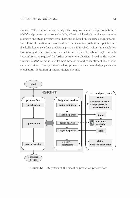
3.4 PROCESS INTEGRATION 61
module. When the optimization algorithm requires a new design evaluation, a
Matlab script is started automatically by iSight which calculates the new annulus
geometry and stage pressure ratio distribution based on the new design parame-
ters. This information is transferred into the meanline prediction input file and
the Rolls-Royce meanline prediction program is invoked. After the calculation
has converged, the results are bundled in an output file, where iSight extracts
basic information required for further parameter evaluation. Based on the results,
a second Matlab script is used for post-processing and calculation of the criteria
and constraints. The optimization loop proceeds with a new design parameter
vector until the desired optimized design is found.
iSight file parser input
iSight file parser
objectives
constraints
design analysismeanline
prediction
output
• annulus line calc.
• stage pressure
ratio distribution
Matlab
• criteria calculation
Matlab
post-processing
external programs
start
optimized
design
optimization
design definition
process flow
initialization
design evaluation
Figure 3.4: Integration of the meanline prediction process flow

62 3 OPTIMIZATION BASED PRELIMINARY DESIGN
3.5 Results and Discussion
In order to demonstrate the potential of process integration, automation and
multi-objective optimization on preliminary aerodynamic compressor design, the
annulus geometry of a given 9-stage high pressure compressor design is opti-
mized. The goal of this investigation is to find an improved compressor design by
modifying the annulus geometry only, but keeping the inlet and outlet annulus
coordinates constant. In a first investigation the annulus geometry is parame-
terized according to Equations (3.11) and (3.12) with n + 1 = 4 control points,
respectively, leading to a design vector
p =[bMx,1, b
Mx,2, b
My,1, b
My,2, b
Δx,1, b
Δx,2, b
Δy,1, b
Δy,2
]T.
The multi-objective optimization problem (3.10) originally consisting of three
individual objectives is transferred by the compromise method (2.21) to a scalar
optimization problem where the main objective to be maximized is the overall
compressor polytropic efficiency ηc,poly. The surge margin at design point SM
is considered as an inequality constraint with an user-defined lower bound SM ,
and the overall pressure ratio Πc is kept constant since it is determined uniquely
by the given pressure ratio distribution. In order to create feasible solutions, all
design constraints in (3.10) are taken into account resulting in
maxp∈Rn
ηc,poly (3.21)
subject to
maxi
Ψi ≤ Ψ maxi
DFRi ≤ DF
maxi
M ′RI,i ≤ M ′R
I maxi
DF Si ≤ DF
maxi
MSI,i ≤ MS
I mini
DHRi ≥ DH
maxi
Ch,i ≤ Ch mini
DHSi ≥ DH
MSE,Ns
≤ ME SM ≥ SM
with i = 1(1)9
The scalar optimization problem is solved with the Multi-Island Genetic Al-
gorithm, see Section 2.3.4.4, with a population size of 20 individuals on each
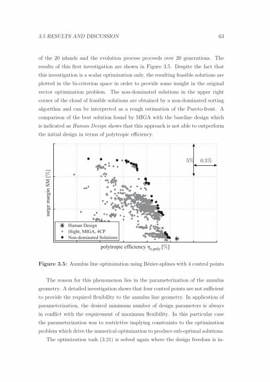
3.5 RESULTS AND DISCUSSION 63
of the 20 islands and the evolution process proceeds over 20 generations. The
results of this first investigation are shown in Figure 3.5. Despite the fact that
this investigation is a scalar optimization only, the resulting feasible solutions are
plotted in the bi-criterion space in order to provide some insight in the original
vector optimization problem. The non-dominated solutions in the upper right
corner of the cloud of feasible solutions are obtained by a non-dominated sorting
algorithm and can be interpreted as a rough estimation of the Pareto-front. A
comparison of the best solution found by MIGA with the baseline design which
is indicated as Human Design shows that this approach is not able to outperform
the initial design in terms of polytropic efficiency.
Human Design
iSight, MIGA, 4CP
Non-dominated Solutions
0.5%5%
polytropic efficiency �c,poly [ ]%
surg
em
argin
SM
[]
%
Figure 3.5: Annulus line optimization using Bezier-splines with 4 control points
The reason for this phenomenon lies in the parameterization of the annulus
geometry. A detailed investigation shows that four control points are not sufficient
to provide the required flexibility to the annulus line geometry. In application of
parameterization, the desired minimum number of design parameters is always
in conflict with the requirement of maximum flexibility. In this particular case
the parameterization was to restrictive implying constraints to the optimization
problem which drive the numerical optimization to produce sub-optimal solutions.
The optimization task (3.21) is solved again where the design freedom is in-
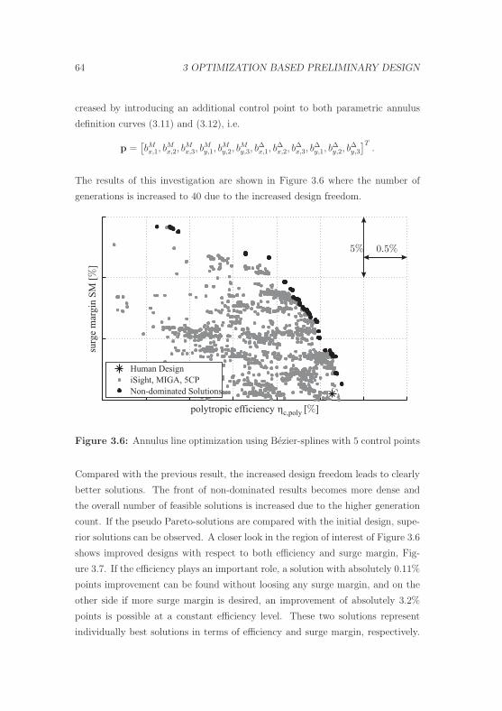
64 3 OPTIMIZATION BASED PRELIMINARY DESIGN
creased by introducing an additional control point to both parametric annulus
definition curves (3.11) and (3.12), i.e.
p =[bMx,1, b
Mx,2, b
Mx,3, b
My,1, b
My,2, b
My,3, b
Δx,1, b
Δx,2, b
Δx,3, b
Δy,1, b
Δy,2, b
Δy,3
]T.
The results of this investigation are shown in Figure 3.6 where the number of
generations is increased to 40 due to the increased design freedom.
Human Design
iSight, MIGA, 5CP
Non-dominated Solutions
polytropic efficiency �c,poly [ ]%
surg
em
argin
SM
[]
%
0.5%5%
Figure 3.6: Annulus line optimization using Bezier-splines with 5 control points
Compared with the previous result, the increased design freedom leads to clearly
better solutions. The front of non-dominated results becomes more dense and
the overall number of feasible solutions is increased due to the higher generation
count. If the pseudo Pareto-solutions are compared with the initial design, supe-
rior solutions can be observed. A closer look in the region of interest of Figure 3.6
shows improved designs with respect to both efficiency and surge margin, Fig-
ure 3.7. If the efficiency plays an important role, a solution with absolutely 0.11%
points improvement can be found without loosing any surge margin, and on the
other side if more surge margin is desired, an improvement of absolutely 3.2%
points is possible at a constant efficiency level. These two solutions represent
individually best solutions in terms of efficiency and surge margin, respectively.

3.5 RESULTS AND DISCUSSION 65
Further solutions exist lying in between of these two points which are slightly
better in both objectives compared to the datum design.
Human Design
iSight, MIGA, 5CP
polytropic efficiency �c,poly [ ]%
surg
em
argin
SM
[]
%
0.1%1%
best surge margin
0.11%
3.2%
best efficiency
Figure 3.7: Optimal trade-off results with MIGA
The result of this investigation looks very promising. The front of non-
dominated solutions offers the design engineer a good basis to discuss on trade-offs
between polytropic efficiency and surge margin. However, it should be reem-
phasized that this investigation is done based on a single-objective optimization
algorithm only and obviously it can not be expected that the non-dominated so-
lutions are really representing the Pareto-front. Beside this major problem two
more issues can be addressed. Firstly, the result shown in Figure 3.6 contains
undesired gaps in the non-dominated solution front, and secondly a huge number
of solutions are generated in a region which is not really of interest. Therefore,
it should be the goal to find more solutions at the Pareto-front, to close the gaps
and to avoid undesired solutions.
In order to address these issues, another investigation based on the same annu-
lus line parameterization is done. The optimization problem (3.21) is solved again
using the gradient based algorithm NLPQL, see Section 2.3.4.4. The difference
between this approach and the previous one is that 40 individual optimizations
are performed with an increasing lower bound on the surge margin SM in order

66 3 OPTIMIZATION BASED PRELIMINARY DESIGN
to create a more dense non-dominated solution front. All individual optimization
runs are started from the same initial human design point. The overall compres-
sor pressure ratio, as the third objective, is kept invariant due to a constant stage
pressure ratio distribution which makes this investigation comparable with the
previous one.
Figure 3.8 shows the feasible solutions obtained by all 40 individual NLPQL
optimization runs. It can be seen that the gradient based algorithm produces
solutions closer to the Pareto-front. Compared with the MIGA investigation the
solutions are significantly improved and due to the application of the compromise
method with moving bound a clearly better Pareto-front can be observed. Fur-
thermore, the gaps within the frontier are reduced which is basically driven by
the small step sizes of the inequality surge margin constraint. This is basically
an important point in terms of discussing trade-off solutions.
Human Design
iSight, MIGA, 5CP
iSight, NLPQL, 5CP
Pareto-optimal Designs
polytropic efficiency �c,poly [ ]%
surg
em
argin
SM
[]
%
0.5%5%
Figure 3.8: NLPQL results in comparison with MIGA
The improvement of the annulus design can be better seen in Figure 3.9 where
the design engineer can choose between a compressor design with an increased
polytropic efficiency by 0.16% points at constant surge margin, a design which
has a 4.4% points higher surge margin at the equal efficiency level, or one of the
well distributed trade-offs with better surge margin and efficiency.

3.5 RESULTS AND DISCUSSION 67
Human Design
iSight, NLPQL, 5CP
polytropic efficiency �c,poly [ ]%
surg
em
argin
SM
[]
%
0.1%
1%
best surge margin
best efficiency
0.16%
4.4%
Figure 3.9: Pareto-optimal results with NLPQL
Summarizing, Figure 3.10 compares the non-dominated solution fronts for the
presented three investigations. In general one can say that the optimal solutions
found by the deterministic method are obviously more reliable than results from
the stochastic approach and that the solution depends significantly on the design
freedom. It is obvious that additional control points to the annuls line parame-
terization lead to more flexibility and thus to better designs, however, from the
practical point of view a trade-off between flexibility and computational costs has
to be found.
It should be mentioned that more competitive Pareto-fronts would be deter-
mined by the stochastic approach if the MIGA algorithm would be repeated by
means of the compromise method with variable surge margin steps. However, in
general genetic algorithms need too many function evaluations and the determina-
tion of the Pareto-front would be too expensive in term of overall computational
time.

68 3 OPTIMIZATION BASED PRELIMINARY DESIGN
Human Design
iSight, MIGA, 4CP
iSight, MIGA, 5CP
iSight, NLPQL, 5CP
polytropic efficiency �c,poly [ ]%
surg
em
argin
SM
[]
%
0.5%5%
Figure 3.10: Comparison of non-dominated solutions
As mentioned before, the annulus geometry optimization is obviously one of
the key elements in compressor preliminary design especially due to the number
of design parameters and the requirements for smoothness which always have
to be considered. Nevertheless, the performance of the compressor depends also
on other parameter values and especially on their appropriate distribution along
the compressor mid-height. Hence, in a further investigation the stage pressure
ratio distribution as an additional design quantity beside the annulus geometry
is introduced. In order to guarantee required smoothness, the stage pressure
ratio distribution is also parameterized by a Bezier-curve with five control points
according to Equation (3.19) which can be also seen in Figure 3.3. The number
of design parameters rises up to 20 consisting of 12 for the parametric annulus
description and 8 for the stage pressure ratio distribution, i.e.
p =[bMx,1, b
Mx,2, b
Mx,3, b
My,1, b
My,2, b
My,3, b
Δx,1, b
Δx,2, b
Δx,3, b
Δy,1, b
Δy,2, b
Δy,3, . . .
. . . , bΠx,1, b
Πx,2, b
Πx,3, b
Πy,0, b
Πy,1, b
Πy,2, b
Πy,3, b
Πy,4
]T.
The multi-objective optimization problem (3.10) is solved by using the overall
polytropic efficiency as solely objective and transferring the surge margin to an

3.5 RESULTS AND DISCUSSION 69
inequality constraint with a single lower bound SM . In this particular case the
overall compressor pressure ratio Πc is not restricted to the desired quantity rather
it is just calculated by Equation (A.8) depending on the individual stage pressure
values according to their distribution. However, restrictions of the control point
positions for the stage pressure ratio parameterization is necessary in order to
obtain feasible solutions. The multi-objective optimization problem (3.10) is then
transferred by the compromise method as
maxp∈Rn
ηc,poly (3.22)
subject to
maxi
Ψi ≤ Ψ maxi
DFRi ≤ DF
maxi
M ′RI,i ≤ M ′R
I maxi
DF Si ≤ DF
maxi
MSI,i ≤ MS
I mini
DHRi ≥ DH
maxi
Ch,i ≤ Ch mini
DHSi ≥ DH
MSE,Ns
≤ ME SM ≥ SM
2 ≥ bΠy,k ≥ 1, with i = 1(1)9, k = 1(1)5
Figure 3.11 shows the feasible solutions in the criterion space obtained by
the genetic algorithm MIGA. Due to the increased design freedom the number of
function evaluations is adopted to a population size of 30 individuals distributed
on each of the 30 islands and evolved over 60 generations. The results of the
three-criterion problem are shown in a two-dimensional plot where the overall
pressure ratio as the third criterion is indicated by the color.
The amount of function evaluations leads to a high number of feasible solutions
which are distributed within the criterion space. The improvement of overall
pressure ratio for reduced efficiency levels is a confirmation for the contradiction
of the objectives. A further interesting point here is that compressor designs exist
where this improvement is correlated with higher surge margin values. These
results can be used to understand the design problem better and to find new
innovative solutions. In order to quantify the goodness of this investigation, the
solutions may be compared with the datum design. A closer look around the
datum design and a filtering of the results with respect to surge margin and

70 3 OPTIMIZATION BASED PRELIMINARY DESIGN
Human DesigniSight, MIGA, 5CP
polytropic efficiency ηc,poly [%]
surg
em
argi
nSM
[%]
Πc
0.5%5%
Figure 3.11: Multi-criterion optimization with respect to efficiency, surge mar-
gin and overall pressure ratio
overall pressure ratio based on the datum design values shows that improved
designs with respect to all three objectives can be found, Figure 3.12.
In Figure 3.13 the annulus geometries as well as the stage pressure ratio dis-
tributions for three extreme designs from Figure 3.12 are shown. The maximum
efficiency design shows an unload of the first stage which is covered by the last
three stages. The overall pressure ratio and surge margin are quite similar to the
initial design and the efficiency is improved by 0.16% points. For the second case
the surge margin is increased by 4.9% points at reasonable efficiency values and
the overall pressure ratio is also slightly improved. In the last case a reduction of
the stage pressure ratio at the three front stages and an increase of other stages
can be observed which leads to an improvement of 2% in overall pressure ratio in
comparison to the datum design without loosing surge margin and efficiency. In
comparison with the initial design it can be recognized that all annulus geome-
tries differ form each other. In particular the front region is characterized by a
higher annulus height and the rear part by an increased radial coordinate of the
mid-height line. From the corresponding stage pressure ratio plots in general a
redistribution of the loading is visible.
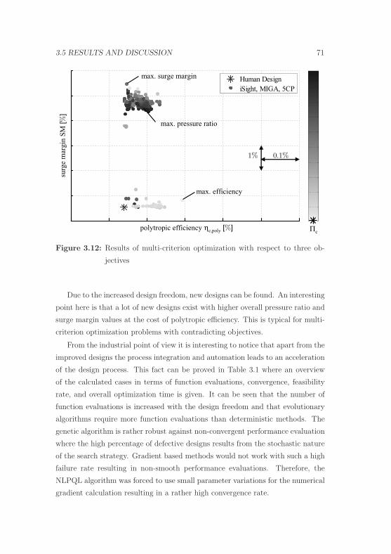
3.5 RESULTS AND DISCUSSION 71
Human DesigniSight, MIGA, 5CP
polytropic efficiency ηc,poly [%]
surg
em
argi
nSM
[%]
Πc
0.1%1%
max. efficiency
max. pressure ratio
max. surge margin
Figure 3.12: Results of multi-criterion optimization with respect to three ob-
jectives
Due to the increased design freedom, new designs can be found. An interesting
point here is that a lot of new designs exist with higher overall pressure ratio and
surge margin values at the cost of polytropic efficiency. This is typical for multi-
criterion optimization problems with contradicting objectives.
From the industrial point of view it is interesting to notice that apart from the
improved designs the process integration and automation leads to an acceleration
of the design process. This fact can be proved in Table 3.1 where an overview
of the calculated cases in terms of function evaluations, convergence, feasibility
rate, and overall optimization time is given. It can be seen that the number of
function evaluations is increased with the design freedom and that evolutionary
algorithms require more function evaluations than deterministic methods. The
genetic algorithm is rather robust against non-convergent performance evaluation
where the high percentage of defective designs results from the stochastic nature
of the search strategy. Gradient based methods would not work with such a high
failure rate resulting in non-smooth performance evaluations. Therefore, the
NLPQL algorithm was forced to use small parameter variations for the numerical
gradient calculation resulting in a rather high convergence rate.
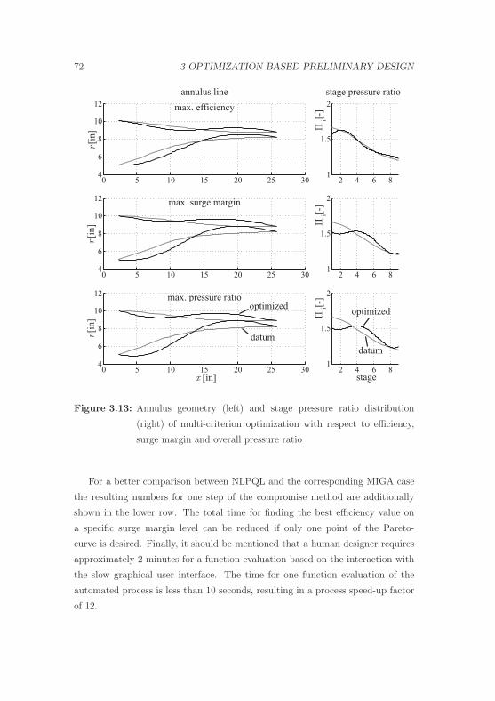
72 3 OPTIMIZATION BASED PRELIMINARY DESIGN
2 4 6 81
1.5
2
0 5 10 15 20 25 304
6
8
10
12
x [in]
r[i
n] �
i[-]
2 4 6 81
1.5
2
0 5 10 15 20 25 304
6
8
10
12
2 4 6 81
1.5
2
0 5 10 15 20 25 304
6
8
10
12
r[i
n]
r[i
n]
�i[-
]�
i[-]
optimized
datum
optimized
datum
stage
stage pressure ratio
max. efficiency
max. surge margin
max. pressure ratio
annulus line
Figure 3.13: Annulus geometry (left) and stage pressure ratio distribution
(right) of multi-criterion optimization with respect to efficiency,
surge margin and overall pressure ratio
For a better comparison between NLPQL and the corresponding MIGA case
the resulting numbers for one step of the compromise method are additionally
shown in the lower row. The total time for finding the best efficiency value on
a specific surge margin level can be reduced if only one point of the Pareto-
curve is desired. Finally, it should be mentioned that a human designer requires
approximately 2 minutes for a function evaluation based on the interaction with
the slow graphical user interface. The time for one function evaluation of the
automated process is less than 10 seconds, resulting in a process speed-up factor
of 12.

3.5 RESULTS AND DISCUSSION 73
Table 3.1: Function evaluation and optimization time for meanline process
function converged feasible total timeevals solutions solutions [h]
MIGA (annulus, 4CP) 8000 90% 58% 19.3
MIGA (annulus, 5CP) 16000 86% 40% 30.5
NLPQL (annulus, 5CP) 10768 99% 8% 18.2
MIGA (annulus+Π, 5CP) 54000 79% 28% 94.1
NLPQL (annulus, 5CP)
1 compromise step 151 100% 24% 0.28
During post-processing a surprising issue with the surge margin prediction of
the meanline analysis tool was detected. It turned out that the correlation based
prediction of the design point surge margin is not valid for geometry variations
as performed in the presented investigations. Therefore, the preliminary design
process was extended by an additional evaluation step. For each design multiple
meanline prediction calculations with variable compressor exit pressure values are
performed in order to determine the design speed characteristic of the compressor
from which the surge margin value is extracted according to Equation (A.12). The
determination of the compressor design point efficiency as an objective of the
optimization process is also based on the results of the characteristic calculation.
In a first investigation the multi-objective optimization design problem (3.21)
is solved based on the NLPQL algorithm as part of the compromise method
consisting of 25 inequality surge margin steps where design variations are made
by annulus geometry modifications only. Figure 3.14 shows all feasible results in
the criterion space and furthermore the obtained non-dominated solutions after a
sorting algorithm. The values for surge margin and efficiency of the datum design
are shown which are also determined with the same new calculation approach in
order to make the solutions comparable with each other. It can be seen that
NLPQL produces a lot of better solutions compared with the datum design in
term of polytropic efficiency as well as for surge margin values and that trade-offs
between the two objectives can be made.

74 3 OPTIMIZATION BASED PRELIMINARY DESIGN
Human Design
iSight, NLPQL, 5CP
Non-dominated Solutions
polytropic efficiency �c,poly [ ]%
surg
em
argin
SM
[]
%
0.05%1%
Figure 3.14: NLPQL results for extended process in comparison with datum
design
A closer look around the human design is given in Figure 3.15 where an
improvement in efficiency of about 0.12% points is achieved without loosing any
surge margin or an increase in surge margin of 2.1% points at an equal efficiency
level. A comparison with the previous investigation based on the former surge
margin definition, Figure 3.9, shows that the relative improvement in efficiency
is fairly similar whereas the improvement in surge margin is reduced. The reason
for this is due to the new definition of the surge margin, however, the trend in
the improvement is also repeated for both objectives in this investigation.
Obviously, the drawback of the extended process is that the overall evaluation
time is slightly higher due to additional calculations required for the surge margin.
However, the new definition is not correlation based anymore and the whole
design speed characteristic is available for postprocessing. Figure 3.16 shows a
comparison of the design speed characteristics between the datum design with the
best efficiency and best surge margin points from Figure 3.15. If we concentrate
on the pressure ratio distributions, Figure 3.16b, it can be observed that all
three curves are intersecting each other at the design point which means that
the flow function and the pressure ratio at the design point is equal as it is
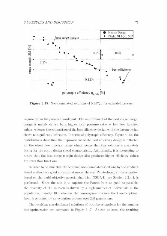
3.5 RESULTS AND DISCUSSION 75
Human Design
iSight, NLPQL, 5CP
polytropic efficiency �c,poly [ ]%
surg
em
argin
SM
[]
%
0.05%0.5%
best surge margin
best efficiency
0.12%
2.1%
Figure 3.15: Non-dominated solutions of NLPQL for extended process
required from the pressure constraint. The improvement of the best surge margin
design is mainly driven by a higher total pressure ratio at low flow function
values, whereas the comparison of the best efficiency design with the datum design
shows no significant deflection. In terms of polytropic efficiency, Figure 3.16a, the
distributions show that the improvement of the best efficiency design is reflected
for the whole flow function range which means that this solution is absolutely
better for the entire design speed characteristic. Additionally, it is interesting to
notice that the best surge margin design also produces higher efficiency values
for lower flow functions.
In order to be sure that the obtained non-dominated solutions by the gradient
based method are good approximations of the real Pareto-front, an investigation
based on the multi-objective genetic algorithm NSGA-II, see Section 2.3.4.4, is
performed. Since the aim is to capture the Pareto-front as good as possible,
the diversity of the solution is driven by a high number of individuals in the
population, namely 100, whereas the convergence towards the Pareto-optimal
front is obtained by an evolution process over 200 generations.
The resulting non-dominated solutions of both investigations for the annulus
line optimization are compared in Figure 3.17. As can be seen, the resulting

76 3 OPTIMIZATION BASED PRELIMINARY DESIGN
Design Point
Datum Design
NLPQL, SM optimized
NLPQL, �c,poly
optimized
flow function FLF [kgK Pa ]0.5 -1
0.51%
0.52
(a)
(b)
pre
ssure
rati
o[-
]�
cpoly
.ef
fici
ency
[]
��
c,p
oly
Figure 3.16: Comparison of polytropic efficiency (a) and pressure ratio (b) dis-
tributions
points are well distributed and both non-dominated frontiers are lying very close
to each other. The biggest deflection can be found for low efficiencies where the
genetic algorithm obtains about 0.5% points higher surge margin values compared
to the gradient based method. It can be generally observed that the NSGA-II
produces better solutions and hence it outperforms NLPQL. This holds true for
the optimization performance, however, if the optimization time and the num-
ber of required function evaluations are considered, the trend turns towards the
gradient based method which is shown in Table 3.2.
Comparing the number of function evaluations shows that the gradient based
approach is much quicker reflected by only 28% function evaluations of the genetic
algorithm. The number of converged solutions are quite similar whereas NLPQL
produces less feasible solutions as known from the previous investigation. From
the industrial point of view the process performance is of major importance which
is reflected by the total optimization time which shows that the gradient based
method is faster than the genetic algorithm by a factor of 3.6. Hence, if the
analysis tools are robust, i.e their convergence rate is high, and the design space
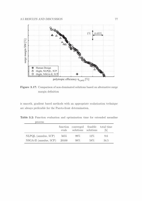
3.5 RESULTS AND DISCUSSION 77
Human Design
iSight, NLPQL, 5CP
iSight, NSGA-II, 5CP
polytropic efficiency �c,poly [ ]%
surg
em
argin
SM
[]
%
0.05%1%
Figure 3.17: Comparison of non-dominated solutions based on alternative surge
margin definition
is smooth, gradient based methods with an appropriate scalarization technique
are always preferable for the Pareto-front determination.
Table 3.2: Function evaluation and optimization time for extended meanline
process
function converged feasible total timeevals solutions solutions [h]
NLPQL (annulus, 5CP) 5655 99% 12% 9.6
NSGA-II (annulus, 5CP) 20100 98% 58% 34.5

4 Optimization Applied to
Throughflow Calculation
The throughflow calculation is an extension of the previous meanline calculation
in radial direction. It requires more calculation time and is too complex to be
fully integrated in an optimization process. Therefore, the throughflow off-design
calculation as a subproblem of the throughflow process is taken as a demon-
stration how process integration and optimization can be applied to industrial
design problems for solving typical time-consuming design tasks. The emphasis
is to accelerate the throughflow off-design process and to provide automated opti-
mization methods and techniques for finding solutions which support the human
engineer.
4.1 Introduction
The throughflow calculation is the second step within the aerodynamic compres-
sor design process. In this design phase appropriate radial distributions of flow
parameters in the meridional plane have to be found which fulfill the overall
compressor requirements. For this reason the results of the meanline prediction
calculation are used as initial solution to the throughflow calculation. Parame-
ters along the mid-height line as blade solidities, losses, stage pressure ratios,
and flow angles are expanded at specific axial positions in radial direction based
on engineering expertise and design rules. The annulus geometry as well as the
predicted blockage distribution are also transferred into the new design model.
Throughflow equations for the flow in a compressor or turbine can be solved
78

4.1 INTRODUCTION 79
with a streamline curvature method. The central part of this method involves
the radial equilibrium equation which is a non-linear ordinary differential equa-
tion relating the radial static pressure gradient of a general swirling flow to the
streamline geometry. In the early use of this equation simplifying assumptions
had to be made in order to integrate it analytically. However, with the devel-
opment of high speed computers it has become possible to solve the equation
using a streamline curvature method without the very restrictive simplifications
needed before. In the streamline curvature method the radial equilibrium equa-
tion is solved iteratively once the inlet mass flow, the blockage assumption, and
the annulus geometry is given. Basically, the throughflow calculation starts with
an approximation of the streamline geometry on 7 to 21 radial positions. The
static pressure is obtained by integrating the radial equilibrium equation which
is then used to derive a new approximation to the streamline geometry. This
iterative procedure is repeated until the result converges and the flow field in the
S2 plane is obtained. The results of the throughflow calculation process are on
one hand radially distributed aerodynamic parameters at each axial blade inlet
and outlet position and on the other hand the streamline distribution itself within
the annulus geometry.
Once, the design throughflow calculation is performed, operating phases re-
flecting take-off or climb situations have to be investigated in order to judge the
feasibility and reliability of the compressor design at off-design flight conditions.
The overall performance requirements for the compressor at these conditions are
a priori given and have to be fulfilled by making assumptions on blade losses and
blade exit whirl angle deflections.
Figure 4.1 shows the general work flow for obtaining an off-design throughflow
solution. The process starts with a necessary design point throughflow calculation
which is used as an initial solution to the off-design problem. Thereupon the
engineer has to apply the off-design conditions which include the off-design shaft
speed, inlet total temperature, inlet total pressure, and inlet mass flow. If bleeds
and variable stators exist in the compressor design, the bleed air mass flow as well
as the variable stator angles have to be adapted to the design problem too. The
next step is to run the throughflow calculation with these off-design parameter
settings. Unfortunately, in some cases where the off-design is far away from the
initial design point solution, it may happen that the throughflow calculation does

80 4 OPTIMIZATION APPLIED TO THROUGHFLOW CALCULATION
not converge. The reason for this is that the blade loss and exit whirl angle
assumptions are not set properly to the problem.
The problem in such a case is that no solution file exists from which objective
function values could be extracted. Therefore, it is necessary to use the inlet
mass flow as a temporary design parameter in order to achieve some intermediate
converged off-design solution. Since the calculation converges, objective values
can be extracted and compared with the required compressor performance data.
During the off-design solution finding process, obviously, the inlet mass flow has
to be driven back to the correct value.
Application ofOff-Design Flow
Conditions
Throughflow DesignPoint Calculation
Off-DesignCalculation
Converged?no Adjust Compressor
Inlet Mass Flow
PerformanceValues Achieved?
no Adjust DesignParameters
yes
yes
Off-DesignFinished
Figure 4.1: Off-design preparation

4.2 OFF-DESIGN OPTIMIZATION PROBLEM 81
The throughflow off-design calculation is a highly iterative process which can
be accelerated by means of process integration and automation. In order to fulfill
the multiple performance requirements, the throughflow off-design problem can
be formulated as a multi-objective design problem.
4.2 Off-Design Optimization Problem
The throughflow off-design problem can be transferred into a rather small opti-
mization problem consisting of two design variables and three objectives. The
first design parameter reflects the increase or in some specific cases the decrease
of the pressure losses at each blade row at off-design flow conditions. It is de-
fined as an additional loss assumption factor χ ∈ R which is multiplied on all
rotor and stator blade radial loss distributions, respectively. The second design
parameter describes the change in exit flow angle also caused by off-design flow
conditions. The parameter is denoted by ΔD ∈ R and it is assumed that the
deflection is radially constant and equal for all rotor and stator blade rows. Both
design parameters are typically restricted by user defined bounds in order to avoid
convergence problems of the throughflow calculation program due to physically
unrealistic values. Summarizing, the design vector for the throughflow off-design
calculation process can be expressed by
p = [χ, ΔD]T .
As already mentioned, the aim of the throughflow off-design calculation
process is to match required performance parameters. These parameters are the
overall compressor pressure ratio Πc, the isentropic compressor efficiency ηc,isen
and the compressor exit total temperature T0,c,E. Due to the fact that it is often
not possible to hit all three values exactly, an off-design calculation is being ac-
cepted when the difference in polytropic efficiency and overall compressor pressure
ratio is less or equal 1% and the deflection in compressor exit total temperature
is less or equal 1K compared to the given performance values. The objectives of
the throughflow off-design calculation can be formulated in such a way that all
three terms are in the same order of magnitude. The first objective

82 4 OPTIMIZATION APPLIED TO THROUGHFLOW CALCULATION
Πc =ΔΠc
Πc
· 100% (4.1)
describes the relative deviation of the overall compressor pressure ratio from the
required value, the second objective
ηc,isen =Δηc,isen
ηc,isen
· 100% (4.2)
describes the relative deviation of the isentropic compressor efficiency, and the
third objective
T0,c,E = ΔT0,c,E (4.3)
uses the absolute deviation of the compressor total exit temperature. Summariz-
ing, the multi-objective throughflow off-design problem can be expressed by
minp∈Rn
⎡⎢⎢⎢⎣Πc
ηc,isen
T0,c,E
⎤⎥⎥⎥⎦ (4.4)
subject to
χl ≤ χ ≤ χu
ΔDl ≤ ΔD ≤ ΔDu
with upper and lower bounds for the design parameters.
4.3 Throughflow Off-Design Process Integra-
tion
The Rolls-Royce off-design calculation process is also integrated in an automated
environment using iSight as process integration and automation tool, Figure 4.2.

4.3 THROUGHFLOW OFF-DESIGN PROCESS INTEGRATION 83
The process starts based on a design throughflow solution where the new design
conditions have to be applied a priori according to the off-design case in an
initialization process. The chosen optimization algorithm provides a set of design
parameters p which are parsed in the throughflow input file and the throughflow
calculation program is invoked. The results are written in an output file from
which the objective function values are extracted. If the required performance
values are not achieved, the next optimization step starts with a new design
vector p.
external programs
iSight file parser input
iSight file parser
objectives
constraints
design analysisthroughflow
calculation
output
post-processing
start
optimized
design
optimization
process flow
initialization
design evaluation
Figure 4.2: Integration of the throughflow off-design process flow
For some off-design cases where the convergence rate of the throughflow calcu-
lation is very low, it is required to firstly use a pattern method, which explores the
design space for a promising point from where the overall optimization process
can start. Especially, if the calculations do not converge around the starting point
this step becomes essential for gradient based algorithms, because non-converged

84 4 OPTIMIZATION APPLIED TO THROUGHFLOW CALCULATION
calculations do not provide any confident information and hence the determina-
tion of gradient information becomes very problematic. Furthermore, if a good
starting point is used the chance of finding the global optimum increases for any
deterministic method. If a pattern method is desired in the automated through-
flow off-design calculation process, it can be simply chosen in the process flow
environment of iSight.
4.4 Results and Discussion
In this section results of a throughflow off-design problem based on a 6-stage high
pressure compressor model with five bleed positions and two variable stator blade
rows are presented. All investigations are run at maximum take-off operating
conditions and differ basically with respect to the objective function definition.
Due to the fact that the off-design case converges properly in a wide range of the
design space, the gradient based algorithm NLPQL is chosen and the required
gradients for the search direction are calculated numerically based on forward
differences with an appropriate small parameter perturbation. The pressure loss
coefficient factor χ and the additional exit whirl angle ΔD are bounded by
0.5 ≤ χ ≤ 1.5
1◦ ≤ ΔD ≤ 2◦
In the first investigation the off-design throughflow problem is solved by trans-
ferring the multi-objective problem (4.4) to a single-objective problem using the
weighted-objective scalarization approach (2.19). Since the individual objectives
may become negative, absolute values are considered which makes the approach
equivalent to the distance method with the metric r = 1, see Section 2.3.3.2. The
new compound function F to be minimized reads as
minp∈R2
F (p) (4.5)
with F (p) =∣∣∣Πc
∣∣∣+ |ηc,isen| +∣∣∣T0,c,E
∣∣∣ .Taking absolute values implies non-smoothness in the objective function which
can lead to convergence problems of the optimization algorithm. Hence, a second

4.4 RESULTS AND DISCUSSION 85
investigation with a smooth objective function F is run by means of the distance
method (2.20) with the metric r = 2, i.e.
minp∈R2
F (p) (4.6)
with F (p) =
√(Πc
)2
+ (ηc,isen)2 +(T0,c,E
)2
.
In order to find the best approach for the throughflow off-design optimization,
a third investigation based on the min-max method (2.22) is performed. An
artificial parameter γ is introduced as new objective and the original ones are
considered as inequality constraints bounded by γ. Since it is also a design
variable, the design parameter space is enlarged, i.e. p = [χ, ΔD, γ]T , leading to
the min-max optimization problem
minp∈R3
γ
subject to ∣∣∣Πc
∣∣∣ ≤ γ
|ηc,isen| ≤ γ∣∣∣T0,c,E
∣∣∣ ≤ γ.
(4.7)
The results of all three investigations, denoted by case 1 to case 3, are sum-
marized in Table 4.1. For a general comparison two major aspects can be distin-
guished: the process performance described by the required number of function
evaluations, feasible solutions and overall optimization time, and the optimization
performance indicated by the obtained optimization solutions.
It can be seen, that all three formulations are able to solve the throughflow
off-design problem properly. If we compare the process performance of the three
cases, only small differences are identifiable. The number of required function
evaluations is fairly equal, but case 3 produces less feasible solutions during the
optimization procedure which is mainly driven by the additional constraints of
the min-max formulation, and has no influence on the overall optimization time.
If we compare the process performance, no favorite can be declared. The opti-
mization performance which is reflected by the best obtained solution shows that

86 4 OPTIMIZATION APPLIED TO THROUGHFLOW CALCULATION
the min-max formulation yields very low values for all three objective functions.
Compared to the human design, it outperforms the manual search procedure sig-
nificantly. The weighted-objective method as well as the distance method show
improvements in the efficiency and temperature criteria compared to the human
design, while the total pressure ratio could not be improved. Hence, both ap-
proaches provide trade-off solutions to the multi-objective throughflow off-design
problem.
In order to judge the process acceleration and the quality of the final solutions,
results achieved by a manual search procedure of a human design engineer are also
shown in the table. It can be seen that the min-max formulation is significantly
better in terms of process performance and optimization performance. Despite
the fact that the automated optimization processes require twice more function
evaluations as the human engineer, the overall process time is reduced for all
three cases by more than 80%. The reason for this lies in the acceleration of
the time consuming throughflow input file preparation by the automated parsing
functionality of iSight.
Table 4.1: Function evaluation and optimization time for throughflow off-design
calculation
human case 1 case 2 case 3 case 4engineer (weighted-obj.) (distance) (min-max)
function evals 23 46 44 43 21
feasible runs - 44 42 19 19
total time [h] 8.0 1.52 1.42 1.40 0.67
time/eval [min] 20.87 1.98 1.94 1.95 1.91∣∣∣Πc
∣∣∣ [%] 0.220 0.653 0.334 0.048 0.446
|ηc,isen| [%] 0.530 0.336 0.035 0.069 0.069∣∣∣T0,c,E
∣∣∣ [K] 0.830 0.030 0.230 0.060 0.810
optimal χ 1.020 0.945 0.964 0.970 0.972
design ΔD -0.590 -0.633 -0.590 -0.582 -0.567
At this point it should be mentioned that this comparison is not really fair.
In the three investigated cases the optimization algorithm is seeking for the best

4.4 RESULTS AND DISCUSSION 87
solution to the problem where the human engineer usually stops his search at
the point where all three objective values are below the required bounds. Hence,
a fourth investigation is performed on the basis of the distance method (4.6)
where the optimization procedure is stopped according to the same bounds being
used by the human engineer. The results of case 4 shows that the number of
required function evaluations can be reduced which has a positiv influence on
the process performance. A comparison with the original case 2 shows that
using the stopping criteria saves 53% computational time. The more interesting
comparison, however, is between the solutions of the human engineer and case 4.
Here, the process performance is increased and the overall computational time is
reduced by 92% which is equivalent to a process acceleration factor of 12.
A further interesting point is the number of required optimization steps where
each consists of search direction determination and the line search procedure.
Figure 4.3 shows that the weighted-objective method requires seven, the distance
method and the min-max formulation six, and the truncated distance method
only four iteration steps, respectively.
0 1 2 3 4 5 6 70
50 case 1
0 1 2 3 4 5 6 70
50 case 2
0 1 2 3 4 5 6 70
50 case 3
0 1 2 3 4 5 6 70
50 case 4
iteration [-]
obje
ctiv
efu
nct
ion
val
ue
F
Figure 4.3: Convergence distribution for throughflow off-design cases
In order to analyze the complexity of this particular off-design problem and

88 4 OPTIMIZATION APPLIED TO THROUGHFLOW CALCULATION
to demonstrate how close the solutions are to each other, a design space matrix is
calculated where both design parameters are modified within their feasible bounds
in 21 equidistant steps. This results in 441 throughflow calculations illustrated
in Figure 4.4 where a converged solution is indicated by a single point and the
corresponding objective function value according to (4.5) by the gray scale. Non-
converged solutions in the right lower corner are indicated by the hatched region.
It can be seen that the design space is pretty smooth with increasing values for the
objective function F in the upper left and lower right corner. Furthermore, a flat
valley can be found with just a single optimum indicating the desired minimum
of the objective function. The solutions of all cases are in the vicinity of this
optimum, and in particular the design vectors for case 2, 3, and 4 are very close
to each other.
pressure loss coefficient factor [-]�
F
addit
ional
exit
whir
lan
gel
[deg
]�
�
case 1
case 2
case 3
human engineer
case 4
Figure 4.4: Throughflow off-design results according to objective (4.5) in the
design space
From the optimization point of view it can be summarized that this through-
flow off-design problem is not very challenging. The obtained results show that
this smooth problem can be solved with elementary scalarization techniques and
the best solution is obtained with the min-max formulation while the computa-

4.4 RESULTS AND DISCUSSION 89
tional costs for seeking the best solution is equivalent for all three techniques.
From an industrial point of view, however, it is interesting to notice that the
engineering work is accelerated significantly by means of process integration and
automation. If additional stopping constraints are introduced to the process in
order to come closer to the real engineering work flow, a further improvement of
the process performance can be observed and the overall process is accelerated
by a factor of 12.
5 Blade Design
The blading process consist of two-dimensional blade section design as well as the
more complex three-dimensional blade geometry generation. From the industrial
point of view it is a rather complex process since it involves a geometry generation
tool and a numerical flow analysis for the determination of the blade geometry.
The emphasis of this chapter is to show possibilities in industrial process integra-
tion and automation for accelerating the time-consuming blading process. Since
in blade design multiple goals have to be pursued simultaneously, the application
of multi-objective optimization is demonstrated based on the stochastic NSGA-II
optimization method. Furthermore, two alternative problem definitions for the
two-dimensional blade design problem will be introduced and discussed which
consider aerodynamic and geometric constraints for the optimization process.
Finally, a method for three-dimensional blade design will be presented which is
based on multiple two-dimensional optimized blade sections.
5.1 Introduction
The blade design process is the final step within the aerodynamic compressor
design. The goal is to find three-dimensional blade geometries for all rotor and
stator blades within the compressor which fulfill the requirements of the previous
throughflow calculation in terms of flow turning with a minimum in loss pro-
duction for defined aerodynamic design and off-design flow conditions. This is
basically one of the most time-consuming and challenging design steps within the
aerodynamic compressor design.
Nowadays, there is no straightforward approach to design three-dimensional
90

5.2 BLADE DESIGN PROBLEM 91
blade geometries directly, since the design freedom is too high and the flow in an
aero engine is too complicated. Even on today’s computers 3D-flow analysis based
on Navier-Stokes equations is too expensive why the three-dimensional blade de-
sign problem is approximated according to Wu (1952) by a set of two-dimensional
design problems defined on several radially distributed axis-symmetric stream sur-
faces S1. In these subtasks two-dimensional blade section geometries have to be
found iteratively which are finally stacked along a specific stacking line in order
to obtain the three-dimensional blade geometry.
It is obvious that the aerodynamic performance of the final airfoils, and there-
fore of the whole compressor design, depends significantly on the design quality
of the individual blade sections. Hence, a major part in today’s engineering work
is related to the iterative two-dimensional blade profile design.
It can be shown that the industrial requirement for automated determination
of blade section geometries can be overcome by implementing the individual de-
sign programs into a common environment. Since the engineering work flow is
integrated and automated, numerical optimization can be used in order to find
appropriate blade geometries with respect to the design targets. Furthermore,
the application of multi-objective optimization can support the engineer in his
decision making by providing trade-off solutions between conflicting objectives.
5.2 Blade Design Problem
The goal of the two-dimensional blade design process is to find blade section
geometries which fulfill the flow turning requirements from the previous design
point throughflow calculation with a minimum loss production at given inlet
flow conditions as inlet velocity cI , inlet flow angle αI , and inlet pressure PI ,
Keskin et al. (2006b). The loss that a blade section produces depends on its
geometry and the inlet flow conditions. As demonstrated in Figure 5.1, the
total pressure loss coefficient ω defined in Equation (A.13) increases for a given
geometry for a deviated inlet flow angle αI as it occurs for different operating
conditions. At design flow conditions α0I the flow around the blade section is
smooth and the loss production is typically rather small. If the flow angle is
reduced the stagnation point moves towards the suction side and the flow around
the leading edge gets highly accelerated. A separating bubble on the pressure side

92 5 BLADE DESIGN
may occur and a further reduction of the flow angle drives the flow to separate
on the pressure side leading to higher losses. On the other side an increase of the
flow angle also produces higher losses due to suction side flow separation.
inlet flow angle �I�
I
0
�0
���I)p
ress
ure
loss
coef
fici
ent
�
�I
�I
�I
choke design stall
Figure 5.1: Pressure loss coefficient distribution for inlet flow angle variation
Hence, blade geometry design pursues multiple design objectives simultane-
ously. The first objective is to minimize the loss ω0 = ω (α0I) at design flow
conditions, where the other objective is to maximize the blade working range
WR defined in such a way that the loss does not exceed a prescribed loss level
ωWR due to inlet flow angle variation, Figure 5.2. This level is typically set to
ωWR = 2ω0.
In order to guarantee feasible blade designs, geometric and aerodynamic con-
straints have to be taken into account during the optimization process. It is of
major importance for the compressor design process that the blade design fulfills
elementary geometric requirements in order to be accepted from the subsequent
stress analysis process and to keep the design iteration with the aerodynamics
as small as possible. Thus, the position of maximum blade thickness PMXC is
bounded by reasonable values, and inequality constraints are defined to keep the
cross section area A and the thickness to chord ratio T/C defined in Figure 5.5
above the values of the datum design, respectively.

5.2 BLADE DESIGN PROBLEM 93
�I[deg]�
I
0
�0
���I)
�[
]%
�WR
�I
R
�I
L
WR
��0
Figure 5.2: Definition of design point loss ω0 and working range WR
From the aerodynamic point of view further design constraints have to be
considered. In order to guarantee constant performance of the following blade
rows, the exit flow angle αE has to be preserved by the new design within an
accuracy of ε = 0.25◦, and the separation that may occur on the blade suction
side has to be avoided. In industrial design the boundary layer shape factor H
which describes the relation between the displacement thickness to the momentum
thickness of the boundary layer is used as a criteria for flow separation where it
is required that the shape factor HSSE on the suction side at the trailing edge is
smaller than 2.5, Castillo et al. (2004).
Summarizing, the multi-objective blade design problem can be formulated as
the minimization of the pressure loss coefficient at design flow conditions ω0 and
the maximization of the working range WR which is equivalent to the minimiza-
tion of (−WR). This has to be achieved by variation of the blade geometry
parameters summarized in the design vector p taking into account geometric and
aerodynamic constraints:
minp∈Rn
⎡⎣ ω0
−WR
⎤⎦ (5.1)

94 5 BLADE DESIGN
subject to
20% ≤ PMXC ≤ 60%
A ≥ Adatum
T/C ≥ [T/C]datum
HSSE ≤ 2.5
αE − αE,datum ≤ 0.25
A big issue of solving the multi-objective two-dimensional blade design prob-
lem (5.1) is the determination of the working range value WR. The standard pro-
cedure is to vary the inlet flow angle αI and to determine the loss curve in order
to find the two intersection points ωL = ω(αL
I
)= ωWR and ωR = ω
(αR
I
)= ωWR.
This, however, requires small changes of the inlet flow angle in order to determine
the loss curve accurately which is leading to a rather time-consuming procedure.
In order to release design evaluation from the need of computing the whole
loss curve and searching for the two intersection points, two alternative meth-
ods for solving the two-dimensional blade design problem can be formulated,
Keskin et al. (2006a). In both formulations only three points on the loss curve
are required. The first objective for all cases is the minimization of the loss ω0
at design inlet flow conditions α0I which is obtained by one single flow analysis.
In the first alternative method the inlet flow angle deviations ΔαLI and ΔαR
I
are introduced as additional artificial design variables defining the flow angles
αLI = α0
I − ΔαLI and αR
I = α0I + ΔαR
I , respectively. The sum ΔαLI + ΔαR
I then
declares the working range value WR. During optimization WR is not necessarily
corresponding with the real working range value of the blade section design,
Figure 5.3. However, a maximization of the working range WR will force the
optimization algorithm to increase the distance between the two points αLI and
αRI and hence pushes the losses ωL = ω
(α0
I − ΔαLI
)and ωR = ω
(α0
I + ΔαRI
)towards the required upper bound ωWR. Thus, for the first approach the blade
design problem (5.1) is redefined as
minp,ΔαR
I ,ΔαLI
⎡⎣ ω (α0I)
− (ΔαL
I + ΔαRI
)⎤⎦ (5.2)

5.2 BLADE DESIGN PROBLEM 95
subject to
20% ≤ PMXC ≤ 60% ΔαLI ≥ 0
A ≥ Adatum ΔαRI ≥ 0
T/C ≥ [T/C]datum ωL ≤ ωWR
HSSE ≤ 2.5 ωR ≤ ωWR
αE − αE,datum ≤ 0.25
where ΔαLI and ΔαR
I have to be bounded in order to guarantee positiv values
and ωL and ωR have to be kept below an user defined tolerance for the upper
working range loss ωWR.
�I[deg]�
I
0
�0
���I)
�[
]%
�WR
�I
R
�I
L
WR
��I
L
��I
R
�L
�R
Figure 5.3: First approach for solving the blade design problem by maximizing
WR = ΔαLI + ΔαR
I at constant working range loss level ωWR
As a second alternative method the blade design problem can be solved by
pre-defining the two inlet flow angle deviations ΔαLI and ΔαR
I according to the
needs on the working range, i.e. WR = ΔαLI + ΔαR
I = const. The design goal
is then to minimize the two losses ωL and ωR as demonstrated in Figure 5.4.
This problem definition has now three objectives which have to be minimized
simultaneously and may be solved by applying the min-max formulation (2.22)
to the minimization of the two outer losses ωL and ωR by introducing γ as an

96 5 BLADE DESIGN
artificial objective:
minp,γ
⎡⎣ ω (α0I)
γ
⎤⎦ (5.3)
subject to
20% ≤ PMXC ≤ 60% ωL ≤ γ
A ≥ Adatum ωR ≤ γ
T/C ≥ [T/C]datum
HSSE ≤ 2.5
αE − αE,datum ≤ 0.25
�I[deg]�
I
0
�0
���I)
�[
]%
�I
R
�I
L
WR=const.
��I
L
��I
R
�L
�R
�
Figure 5.4: Second approach for solving the blade design problem by minimizing
ωL and ωR for given working range WR
It should be noticed that in both alternative methods some drawbacks can
be pointed out. Firstly, the number of design parameters is increased by artifi-
cial parameters which typically increases the number of required function eval-
uations. This, however, is not a real drawback since the significant reduction
to only three required loss point calculations in both definitions accelerates the
determination process of the objective function values tremendously. Moreover,

5.3 BLADE PARAMETERIZATION 97
few more design parameters have a very low influence on the overall optimiza-
tion time, particularly if genetic algorithms are used. It may be also a drawback
that in the alternative definitions the working range values are artificial quantities
which make them not directly comparable with the original definition of the blade
design problem. However, with supplementary effort during the postprocessing
phase this drawback can be covered and comparable working range values can
be provided afterwards. Hence, they are chosen for all following investigations as
both definitions are showing promising properties.
5.3 Blade Parameterization
For the blade parameterization and modification the Rolls-Royce program Para-
blading is used, Grasel et al. (2004). This is a blade geometry generation tool for
describing three-dimensional blade shapes on the basis of radially stacked two-
dimensional blade sections. The blade sections are parameterized on S1 stream
surfaces according to the previous throughflow calculation. The parameterization
is flexible and offers enough design freedom for a large variety of section geome-
tries by a low number of design parameters. Parablading provides an interactive
graphical use interface, but can also be run in batch mode which is important in
terms of process integration and automation.
Each individual blade section is split into four segments consisting of blade
leading and trailing edges plus blade suction and pressure sides. The segments
are joined together at the blend points using tangency conditions, Figure 5.5. In
total 28 parameters are required for describing a complete blade section geometry
with circular edges where the set of parameters can be split into 3 leading edge,
3 trailing edge, 10 suction side, 10 pressure side, and 2 global parameters.
The section build up process starts with the determination of the tangential
angles τSSI , τPS
I at the blend points bSS0 , bPS
0 by trigonometrical relations between
the metal angle βI , wedge angle μI , and the radius rI of the leading edge circle.
As a next step the global parameters, i.e. stagger angle ξ and chord length C, in
combination with the blade exit metal angle βE, exit wedge angle μE, and trailing
edge radius rE are used for the determination of the blend points bSS7 , bPS
7 and
the tangential angles τSSE , τPS
E at the trailing edge. Suction and pressure sides of
the blade sections are parameterized each by a cubic B-spline (2.6) with 8 control

98 5 BLADE DESIGN
points bi, i = 0(1)7, demonstrated for the suction side in Figure 5.6. The control
point bSS0 and bSS
7 are the starting and end points of the curve corresponding to
the B-spline parameters t = 0 and t = 1.
T
A
t
[ ( ), ( )]x t y t�
t = 1
PMXC
C
cE
�E
�E
rE E
,
I
rI
t = 0
cI
�I
�I
I
PS
I
SS E E
SS PS,
�
suction side
pressure side
blend point
Figure 5.5: Blade section parameters
b1
SS
b2
SS
b3
SS
b0SS
b4
SSb
5
SS b6
SS b7
SS
nE
SS
nI
SS
tI
SS
tE
SS
lI
SS
lE
SS
y´x´
Figure 5.6: Blade suction side parameterization within Parablading

5.4 BLADE DESIGN PROCESS 99
The points bSS0 , bSS
1 , and bSS2 are related. Point bSS
0 is the given blend point
connecting the suction side with the leading edge circle while bSS1 is determined
by a free parameter lSSI describing the distance along the tangential direction τSS
I .
The control point bSS2 can be determined by the position of the first two points
and additionally the curvature κSSI = κSS(0) and the stiffness σSS
I = σSS(0) at
the blend point bSS0 where the curvature and the stiffness at each curve position
t can be determined by
κ(t) =x(t)y(t) − x(t)y(t)√
[x(t)2 + y(t)2]3(5.4)
σ(t) =x(t)x(t) + y(t)y(t)√
x(t)2 + y(t)2, (5.5)
Bronstein et al. (2005). In the same way the points bSS5 , bSS
6 , and bSS7 are de-
termined by the trailing edge parameters lSSE , τSS
E , κSSE = κ(1), and σSS
E = σ(1),
respectively. The inner points bSS3 and bSS
4 can be chosen freely by tangential
coordinates tSSI , tSS
E and normal coordinates nSSI , nSS
E in a local x′-y′-coordinate
system. The pressure side control points bPSi , i = 0(1)7, are determined analo-
gously to the suction side procedure.
5.4 Blade Design Process
The two-dimensional blade design process consists basically of two steps, geom-
etry generation and design evaluation. Generally these steps are separated and
performed manually leading to a rather time-consuming design task. As a first
goal of this investigation the bade design process is accelerated and automated
by the use of iSight as a front end and control tool to integrate the two design
programs into one common blading process.
Figure 5.7 illustrates the blading process as it is integrated into the iSight
environment. When the optimization algorithm requires a new design evaluation,
the file parsing functionality in iSight is used in order to substitute values of the
design parameters in the input file of the blade geometry generation program

100 5 BLADE DESIGN
external programs
iSight file parser input
geometry
pre-checker
objectives
constraints
geometry generation
post-processing
start
optimized
design
optimization
process flow
initialization
design evaluation
ParabladingParablading
iSight file parser output
design analysis MisesMises
inputoutputinput
output
Figure 5.7: Illustration of the automated 2D-blade optimization process
Parablading. After the program is invoked, a new geometry is generated according
to the input parameters which is stored in an output file needed for the subsequent
two-dimensional flow simulation code Mises.
Before the time-consuming flow analysis is started, basic geometric parame-
ters are extracted from the Parablading output file and checked if the new blade
geometry fulfills sufficient geometric constraints as for example minimum cross
section area or thickness to chord ratio. If at least one of the geometric constraints
is violated the design process starts again from the beginning with a new blade
section design. This is an important step, since genetic algorithms randomly gen-
erate blade profiles which may violate even elementary properties required for a
smooth flow. Furthermore, this step helps to keep the number of flow simulations

5.4 BLADE DESIGN PROCESS 101
as low as possible which has an positive impact to the overall optimization time.
In case of a well behaving geometry the flow domain is discretized with a
structured H-type computational grid which along the flow consists of 60 grid
lines in the inlet region, 70 grid lines on the blade section surface, and 45 lines in
the outlet region, Figure 5.8. In order to resolve high gradient regions the stream
lines are clustered in the computational domain, i.e. the spacing between grid
lines varies. Across the flow 16 grid lines are used which are clustered towards
the blade surface, and at the leading edge the streamlines are more dense due to
the high local curvature.
16
60
70
45
Figure 5.8: Computational grid used for the numerical flow analysis
The flow around the blade section is calculated with the flow solver Mises,
Drela (1986). It is a zonal approach coupling an inviscid outer flow with viscous
boundary layers over blades and in wakes. The inviscid flow is modeled by the
steady state Euler equations which are solved on a streamline grid of nodes.
Viscous and inviscid flow equations are solved simultaneously with an iterative
Newton-Raphson technique. The turbulence intensity is set to Tu = 4% in

102 5 BLADE DESIGN
order to simulate turbo machinery environment, and the Abu-Ghannam/Shaw
transition model, Abu-Ghannam and Shaw (1980), is used to calculate the free
transition position on suction and pressure side, Youngren and Drela (1991).
The results of the Mises calculation are stored into an output file from which
iSight extracts the required information to evaluate objectives and constraints.
The overall optimization proceeds until an optimal design is found or the maxi-
mum number of function evaluations is achieved. Finally, the results and trade-
offs may be visualized in both the design and the criterion space in order to
support the design engineer in his decision making.
5.5 Results and Discussion
In a first investigation a comparison of the two-dimensional blade design problem
definitions (5.2) and (5.3) is performed according to the process flow in Figure 5.7.
On the basis of an initial Rolls-Royce stator blade mid-section design, geometry
modifications are performed at leading edge and suction side of the blade section
geometry only, resulting in a vector of 12 free design variables
p =[βI , μI , l
SSI , κSS
I , σSSI , tSS
I , nSSI , tSS
E , nSSE , lSS
E , κSSE , σSS
E
]Twhere the leading edge circle radius rI is kept fixed at a reasonable minimum
value. The leading edge and the suction side parameters are chosen due to their
major influence on the blade performance according to engineering experience.
Additionally, parameter reduction as it is performed here keeps the design freedom
small and the required number of function evaluations low. The calculations are
performed with constant inlet flow conditions for both investigated definitions,
Table 5.1, where the outlet parameters are results of the flow analysis which have
to be matched to the predefined outlet flow conditions given by a throughflow
calculation.
The Non-dominated Sorting Genetic Algorithm (NSGA-II), Section 2.3.4.4, is
used with an initial population size of 50 individuals running over 124 generations
which is equivalent to 6200 function evaluations. Each evaluation step requires 3
flow computations with Mises according to the loss evaluation at the three inlet

5.5 RESULTS AND DISCUSSION 103
Table 5.1: Inlet flow conditions for 2D-blading
MI αI ReI P0,I PI cI
value 0.776 46.83 1.1E06 438.7 295.2 310.1
unit [ - ] [deg] [ - ] [kPa] [kPa] [m/s]
flow condition points.
Figure 5.9 shows the admissible designs in the criterion space for the first
design problem (5.2). Altogether these are 40.7% feasible solutions of the 6200
possible design modifications generated by the genetic algorithm which fulfill all
constraints. According to problem definition (5.2) the optimal trade-offs lie at
the upper left border which are indicated as non-dominated solutions. As can be
seen, most of the the designs generated by the optimization algorithm are clearly
better than the datum design, and especially the non-dominated solutions show
clearly better performance with respect to both objectives, loss at design point
and working range.
Datum Design
Solutions, (5.2)
Non-dominated Solutions
0.05%0.5°
design point loss [ ]%�0
work
ing
range
[deg
]W
R
Figure 5.9: Criterion space and non-dominated solutions for blade design prob-
lem (5.2)
In Figure 5.10 the criterion space for the second problem definition (5.3) is
shown. Each point is indicating a feasible solution while according to the problem

104 5 BLADE DESIGN
definition the optimal trade-offs can be found in the lower left corner indicated
as non-dominated solutions. In this case 94.9% of 6200 function evaluations
converged and 51.4% feasible solutions are obtained. It can be seen that the trade-
offs are concentrated in the lower left corner and that the differences are rather
small. Due to the fact that no real Pareto-curve exists it can be assumed that
this problem definition leads to a single optimal solution which corresponds to the
point in the lower left corner. Unfortunately, a direct comparison of the solutions
with the datum design or the results of problem (5.2) is not possible, because
γ is a problem specific value which is not contained in the other definitions.
However, a comparison of the real working range values is possible from which
the improvements in the design can be extracted.
Solutions, (5.3)
Non-dominated Solutions
1%
arti
fici
alpar
amet
er[
]�
�
0.01%
design point loss [ ]%�0
Figure 5.10: Criterion space and non-dominated solutions for blade design prob-
lem (5.3)
Thus, for the non-dominated solution of design problem (5.2) which provides
the highest artificial working range value WR and the solution of (5.3) which
provides the minimum losses, full loss curve calculations are performed. In Fig-
ure 5.11b a comparison of the loss curves of these two non-dominated solutions
with the datum design is shown. It can be seen that both optimized designs show
similar loss distributions with an improvement in working range. At a reasonable

5.5 RESULTS AND DISCUSSION 105
loss level of 4% a working range rise of about 1.0◦ with respect to the datum
design is achieved. Additionally, a reduction of the loss at design point is observ-
able reflected by approximately 6% for both optimized designs. The increased
performance can also be concluded from the higher static pressure rise coefficient
cp =PE − PI
P0,I − PI
(5.6)
with the exit and inlet static pressure PE, PI and the inlet total pressure P0,I
in Figure 5.11a at stall and choke region. A comparison of the blade section
geometries confirms that both optimized designs are very close to each other and
only tiny changes in the geometry can be found, Figure 5.12.
In general, the optimized designs show more front loading reflected by a wider
inlet wedge angle and a position of maximum thickness which is moved towards
the leading edge. If we summarize the results of this first investigation, an im-
provement of a two-dimensional blade section design with respect to working
range and pressure loss has been achieved. Both alternative formulations of the
original blade optimization problem definition show promising results whereby
no clear favorite can be pointed out.
In Table 5.2 an overview of the process performance related parameters is
given. For an equal number of function evaluations, problem definition (5.2)
shows a higher convergence rate which is important in terms of process time.
The reason for this is that each non-converged solution requires more process time
since the flow solver is running until the maximum number of its inner iterations is
reached or for the worst case the flow solver or even the grid generator is crashed.
This effect is substantiated by the lower overall optimization time for problem
definition (5.2) due to its higher convergence rate. Hence, if the process time is
considered in a comparison, definition (5.2) shows slightly better performance.
Table 5.2: Comparison of process performance parameters
function converged feasible total timeevals solutions solutions [h]
definition (5.2) 6200 97.5% 40.7% 88.1
definition (5.3) 6200 94.9% 51.4% 99.7

106 5 BLADE DESIGN
0.3
0.35
0.4
0.45
0.5
0.55
Datum Design
Optimized, (5.2)
Optimized, (5.3)
-4 -2 0 2 4 60
1
2
3
4
5
6
7
incidence angle = -��I
� �I I
0[deg]
pre
ssure
loss
coef
fici
ent
[]
�%
stat
icpre
ssure
rise
[-]
cp
(a)
(b)
Figure 5.11: Comparison of static pressure rise (a) and pressure loss coeffi-
cient (b) between datum design and selected optimized solutions
of problem definition (5.2) and (5.3)
In a second investigation the two-dimensional blade section optimization prob-
lem is solved with an increased number of design freedom. Beside the leading edge
and suctions side parameters, geometry modifications on trailing edge and pres-
sure side are considered. Furthermore, the stagger angle ξ as a global parameter
is part of the new design vector
p =[βI , μI , l
SSI , κSS
I , σSSI , tSS
I , nSSI , tSS
E , nSSE , lSS
E , κSSE , σSS
E , . . .
. . . , lPSI , κPS
I , σPSI , tPS
I , nPSI , tPS
E , nPSE , lPS
E , κPSE , σPS
E , βE, μE, ξ]T

5.5 RESULTS AND DISCUSSION 107
Datum Design
Optimized, (5.2)
Optimized, (5.3)
Figure 5.12: Comparison of datum design with optimized blade section geome-
tries
which consists of 25 design parameters. Again, leading and trailing edge radii
rI , rE are kept fixed during the design process which is performed according to
Figure 5.7. The NSGA-II optimization algorithm is chosen with 50 individuals
in each population while the number of generations is increased to 200 due to
the extended design parameter vector. Optimization problem definition (5.2) is
chosen due to the promising results from the previous investigation.
The results of this investigation are shown in the criterion space, Figure 5.13,
where beside the feasible solutions trade-offs are indicated for comparison with the
datum design. In general, it can be observed that the distribution of the solution
points as well as the position and expansion of the non-dominated solution front
looks very similar to the previous investigation where leading edge and suction
side parameters are modified only, Figure 5.9. A detailed comparison of the
non-dominated solutions of both cases shows that the increased design freedom
on blade modification results in a slightly higher value for the potential working
range.
In order to validate and compare the results of the non-dominated solutions
which provide the highest working range value, the corresponding designs of the
previous and the current investigation are selected and loss curve calculations
are performed within the range of ±10◦ deflection to the datum inlet flow an-

108 5 BLADE DESIGN
Datum Design
Solutions
Non-dominated Solutions
0.05%0.5°
design point loss [ ]%�0
work
ing
range
[deg
]W
R
Figure 5.13: Criterion space and non-dominated solutions for blade section op-
timization with 25 parameters
gle. The resulting pressure rise coefficient and loss distributions are shown in
Figure 5.14 where additionally the results of the datum design are included for
better comparison.
As can be seen, the optimized designs are better with respect to both objec-
tives, working range and loss at the design flow angle, compared with the datum
design. If all blade section parameters can be changed, an increase in static pres-
sure for higher inlet flow angles, i.e. in the stall region, can be achieved. This
is reflected in a gain of working range whereas in the choke region the improve-
ment with respect to the datum design is rather small. In case of leading edge
and suction side geometry modification only, the improvement in working range
is mainly obtained for lower relative inlet flow angles driven by a higher static
pressure rise. In general, the loss curves of both optimized designs are slightly
shifted to each other, but the level of improvement is rather equal. In terms of
loss at design flow angle both show a reduction of about 6% compared to the
datum design whereas the improvement in working range is approximately 1.0◦
at a reasonable working range loss level of ωWR = 4%.
If the resulting blade section geometries are compared, Figure 5.15, only tiny

5.5 RESULTS AND DISCUSSION 109
0.3
0.35
0.4
0.45
0.5
0.55
Datum Design
All Parameters Optimized
Suction Side Optimized
incidence angle = -��I
� �I I
0[deg]
pre
ssure
loss
coef
fici
ent
[]
�%
stat
icpre
ssure
rise
[-]
cp
(a)
-4 -2 0 2 4 60
1
2
3
4
5
6
7
(b)
Figure 5.14: Comparison of static pressure rise (a) and pressure loss coefficient
(b) between datum and optimized designs
deflections in the geometry can be found. Both optimized designs are very close
to each other, in particular the redistribution of the cross section area caused by
a higher inlet wedge angle and the movement of the maximum blade thickness
towards the leading is equivalent. In other words, compared with the datum
design both optimized sections show a more front loaded behavior which is the
reason for the improvement in working range.
This effect can be better seen from a comparison of the isentropic Mach num-
ber distributions, Figure 5.16, which are calculated based on the pressure relation

110 5 BLADE DESIGN
Datum Design
All Parameters Optimized
Suction Side Optimized
Figure 5.15: Comparison of optimized blade section geometry
Misen =
√√√√√√ 2
γ − 1
⎛⎜⎝(P0
P
)γ − 1
γ − 1
⎞⎟⎠ (5.7)
where P is the static pressure on the blade surface, P0 the total pressure and γ the
ratio of specific heat capacities. Each Mach number distribution shows two peaks
close to the blade leading edge which are results of the curvature discontinuity at
the two leading edge blend points, and increasing Mach number values due to flow
acceleration at the blade suction side. It can be observed that both optimized
designs show a stronger flow acceleration on the suction side and hence a higher
Mach number compared to the datum design. It is also fact that the axial position
of this maximum Mach number is located more at the front of the blade section
according to the described geometry modifications. Furthermore, the loading near
the leading edge is increased and decreased in the middle part, while it appears
almost unchanged at the trailing edge. It is interesting to notice that in spite of
the fact that the higher supersonic Mach numbers of both optimized cases cause
more shock losses the overall loss is reduced for both. Generally this investigation
confirms that front-loaded blade designs typically lead to wider working ranges.

5.5 RESULTS AND DISCUSSION 111
0 0.1 0.2 0.3 0.4 0.5 0.6 0.7 0.8 0.9 10.2
0.4
0.6
0.8
1
1.2
Datum Design
All Parameters Optimized
Suction Side Optimized
normalized chord length x/C [-]
isen
tropic
Mac
hnum
ber
[-]
Misen
suction side
pressure side
Figure 5.16: Isentropic Mach number distributions for datum and optimized
blade sections
Summarizing, the results of these two investigations have shown that a com-
pressor blade section can be designed automatically and design improvements
with respect to multiple objectives can be made. The application of a multi-
objective optimization strategy additionally provides multiple solutions which
can be used to discuss trade-offs and from which the design engineer can choose
a solution depending on additional decision criteria.
A complete three-dimensional blade geometry can be found by designing sev-
eral two-dimensional blade sections which are radially stacked. Therefore, it
is obvious to use the demonstrated automated blade design and optimization
process also for finding the other desired blade section geometries. In order to
demonstrate the general feasibility, the presented approach for automated blade
design is applied to further blade sections of the same Rolls-Royce high pressure
compressor stator blade design. In this particular case, the blade is divided into
21 sections starting with section 01 at the hub and ending with section 21 at
the casing, where section 11 describes the mid-section of the blade. Based on
the already optimized mid-section, six further sections are selected for improve-
ment, three between mid-section and hub and three towards the casing where
sections close to hub and casing are avoided due to possible flow solver instabil-
ities. The multi-objective design problem is solved based on problem definition

112 5 BLADE DESIGN
(5.2) with the NSGA-II algorithm where 50 individuals in each population are
treated over 200 generations. All parameters for leading and trailing edge, suc-
tion and pressure side as well as the stagger angle are variable for each section
during the optimization process where the bounds for the design parameters are
selected according to the minimum and maximum values of the datum design.
The boundary conditions for the flow solver are also adapted for each section
optimization.
Figures 5.17 and 5.18 show the resulting static pressure rise coefficient and loss
distributions for the upper sections 17, 15, and 13 as well as for the lower sections
09, 07, and 05, respectively. In general, an improvement in working range and
loss at design flow conditions can be observed for all optimized section designs.
The increase in working range is mainly driven by better choke properties and in
some particular cases even by higher pressure rise at stall. Section 17 shows the
highest working range improvement of approximately 2◦ at a reasonable working
range loss level ωWR = 4% whereas the improvements for the other sections lie
between 0.5◦ and 1.5◦. Furthermore, it can be seen that almost each loss curve
is symmetric around the design inlet flow angle which is an additional property
of the problem definition. Hence, beside the improvement in loss at design flow
conditions, in almost each optimized section a decrease in loss production at
off-design conditions can be observed.
The biggest differences in the loss curves and static pressure rise distribution
can be found on section 05 where the datum design is shifted in horizontal di-
rection, Figure 5.18b. The intention of the design engineer is to gain more stall
margin by a re-definition of the design inlet flow angle in choke direction. This
is a common and very easy method for achieving more stall margin in a manual
compressor blade design process. However, this increases also the losses at de-
sign inlet flow conditions and is not an optimal solution to the design problem.
The optimized section 05 which shows a symmetrical loss distribution around
the design inlet flow angle can be interpreted as a trade-off solution between
lower losses and lower stall margin. If the loss reduction is mainly pursuit, the
current optimized design would be the choice. If more stall margin is desired,
the optimization problem has to be adapted. This, however, is not a big issue
since a simple extension of the optimization problem definition by an additional
constraint would ensure the required value.

5.5 RESULTS AND DISCUSSION 113
��I[deg]
�[
]%
cp
[-]
0.3
0.35
0.4
0.45
0.5
0.55
Datum Design
Optimized, section 17
-6 -4 -2 0 2 4 60
1
2
3
4
5
6
7
(a) Blade section 17
�[
]%
��I[deg]
cp
[-]
0.3
0.35
0.4
0.45
0.5
0.55
Datum Design
Optimized, section 15
-6 -4 -2 0 2 4 60
1
2
3
4
5
6
7
(b) Blade section 15
�[
]%
��I[deg]
cp
[-]
0.3
0.35
0.4
0.45
0.5
0.55
Datum Design
Optimized, section 13
-6 -4 -2 0 2 4 60
1
2
3
4
5
6
7
(c) Blade section 13
�[
]%
��I[deg]
cp
[-]
0.3
0.35
0.4
0.45
0.5
0.55
Datum Design
Optimized, section 09
-6 -4 -2 0 2 4 60
1
2
3
4
5
6
7
(d) Blade section 09
Figure 5.17: Static pressure rise coefficient and loss distribution for selected
blade sections - part 1

114 5 BLADE DESIGN
�[
]%
��I[deg]
cp
[-]
0.3
0.35
0.4
0.45
0.5
0.55
Datum Design
Optimized, section 07
-6 -4 -2 0 2 4 60
1
2
3
4
5
6
7
(a) Blade section 07
�[
]%
cp
[-]
��I[deg]
0.3
0.35
0.4
0.45
0.5
0.55
Datum Design
Optimized, section 05
-6 -4 -2 0 2 4 60
1
2
3
4
5
6
7
(b) Blade section 05
Figure 5.18: Static pressure rise coefficient and loss distribution for selected
blade sections - part 2
Figure 5.19 presents a summary of the radial distributions of the design point
loss ω0 and the working range WR at a comparable working range loss level of
ωWR = 4% for the datum and the seven optimized blade sections. The comparison
shows that the application of automated two-dimensional blade design optimiza-
tion to all blade sections produces promising results. In general, a reduction in
pressure loss at design inlet flow conditions and an increase in working range can
be observed for each optimized blade section design. It should be noticed that
all these results are taken just as one out of a set of non-dominated solutions
which provide various optimal solutions in terms of multi-objective optimization.
The optimal designs in Figure 5.19 represent the best non-dominated solutions
with respect to the working range criteria, however, if the pressure loss at design
point is more important, other optimal design points can be chosen from the set
of available non-dominated solutions resulting in a different radial distribution
for the objective functions.

5.5 RESULTS AND DISCUSSION 115
Datum Design
Optimized1
2
3
4
5
6
7
8
9
10
11
1213
14
15
16
17
18
19
20
21
bla
de
sect
ion
[-]
hub
casing
2°0.5%
(a) (b)
design point loss �0
[ ]� working range WR [deg]
Figure 5.19: Comparison of radial distributions of pressure loss coefficient (a)
and working range (b) at ωWR = 4% for seven optimized blade
sections with datum design
If the optimized blade sections from Figure 5.19 are stacked along a radial
stacking line, a three-dimensional blade geometry is obtained which can be seen in
Figure 5.20. The comparison with the datum design shows that the new geometry
differs significantly. The sections 17, 13, 11, 09, and 05 look rather smooth
whereas sections 15 and 07 produce undesired wiggles in the three-dimensional
blade geometry. In particular, the trailing edge shows the biggest deflection which
is mainly caused by the corresponding stagger angles.
In terms of industrial design, this three-dimensional blade geometry would not
be acceptable since the required radial smoothness is not fulfilled. The reason for
this is that each optimized section is chosen independently based on its maximum
working range value only. Hence, it would be better to select the blade sections
from their set of non-dominated solutions depending on an additional criterion
which considers the neighboring section geometries in order to obtain a smooth
three-dimensional blade design. This is just one simple method which can be
implemented easily in the current process, however, the better approach would

116 5 BLADE DESIGN
optimizeddatum
suction side
pressure side
leadingedge
trailingedge
casing
hub
05
17
11
section
Figure 5.20: Comparison of three-dimensional blade geometry for datum design
(left) and optimized design (right) obtained by seven individual
multi-objective blade section optimization runs
be to consider the required radial smoothness of the blade geometry during the
multi-objective blade optimization process.

6 Conclusions and Outlook
This thesis illustrates some possibilities of process integration and automated op-
timization for supporting the aerodynamic compressor design process. It demon-
strates that time consuming design tasks can be automated and significant reduc-
tions in the overall design cycle time are achievable. In most aerodynamic design
problems multiple contradicting design goals have to be pursuit simultaneously
and many constraints have to be considered. The multi-objective optimization
strategy is a method for solving these kind of problems in an accurate way and
provides trade-off solutions from which the design engineer can choose depend-
ing on his experience and his final decision. It is clear that setting-up the design
process and choosing appropriate optimization algorithms are prerequisite for the
success, and expertise in process definition, problem formulation and optimization
algorithms is essential.
As a first demonstration for the benefits that can be achieved by process inte-
gration and optimization, the highly iterative annulus design task which is part of
the preliminary design process was automated and numerical optimization meth-
ods were performed on the basis of stochastic and deterministic methods. In order
to achieve feasible solutions, constraints on typical compressor design parameters
have been considered. Based on a Rolls-Royce 9-stage high pressure compressor
design, a significant increase in conflicting design objectives, namely efficiency,
surge margin, and overall compressor pressure ratio, as well as an improvement
in process acceleration, resulting in a speed-up factor of 12, are shown. Beside
the process improvements, automated design can find limits and admissibilities
of the problem definition and of the design tools. As an important result of this
investigation, an issue in the reliability of the preliminary analysis tool is pointed
117

118 6 CONCLUSIONS AND OUTLOOK
out. Since the process integration is flexible, an adaption of the automated pre-
liminary design process by including an additional analysis for the determination
of the surge margin value was performed. Non-dominated solutions are achieved
with a deterministic optimization method using the compromise approach and
a stochastic multi-objective optimization algorithm where improvements in com-
pressor efficiency and surge margin can be observed.
The benefits of process integration and automation are presented also on the
throughflow off-design calculation which is a subtask of the throughflow calcula-
tion process. Based on a Rolls-Royce 6-stage high pressure compressor design,
a gradient based optimization algorithm is used to find solutions to the multi-
objective throughflow off-design problem where three different scalarization tech-
niques are applied in order to transfer the multiple goals into a single-objective
design problem. Improved solutions to the design problem are found and the
required design time is accelerated by a factor of 12 compared to the manual
solution finding process.
In the last part of this work the compressor blade design problem was con-
ducted. As an important step the two-dimensional blade design problem was
re-formulated and two alternative problem definitions were provided which are
characterized by a lower number of required function evaluations compared to the
standard procedure. Multi-objective optimizations based on a Rolls-Royce stator
blade mid-height section show promising results with significant improvements in
pressure loss at design flow conditions and working range with a multi-objective
genetic optimizer considering aerodynamic and geometric constraints. The de-
sign process is accelerated by factor of at least 10 since the manual procedure
of finding the working range by at least 30 individual flow calculations is re-
duced to only three points. In a final step a method for three-dimensional blade
design optimization was introduced based on multiple individual blade section
designs. The automated blade design process was applied to further radially dis-
tributed blade sections and improved designs are selected to be compound to a
three-dimensional blade shape.
It is obvious that the aerodynamic compressor design process is too compli-
cated to cover all aspects in this work. From the industrial point of view it is
required to implement more tools and more processes in order to come closer to
the real engineering work flow.

119
In the demonstrated preliminary design process improvements for design point
conditions are achieved only. However, a compressor has to work also for different
operating conditions which makes the design process more complicated. As an
outlook for further work an extension of the presented design tasks by introducing
more design parameters is possible. This increases the design freedom and the
chance to find better solutions to the design problems, but also requires a longer
optimization time or an adaption of the optimization algorithms and strategies.
Furthermore, an extension of the design problems by considering more objectives
and constraints can be done in order to cover additional design aspects in the
preliminary design phase.
The proposed three-dimensional blade design approach based on several ra-
dially stacked optimized blade sections is one possible design method. However,
flow around a blade is highly three-dimensional and very sensitive in term of
surface smoothness which was not considered in the presented approach directly.
As an possible extension of the blading process an additional design criteria for
the blade section determination could be used to guarantee radial smoothness of
the blade geometry. It is also worth to investigate new parameterization meth-
ods describing three-dimensional blade shapes which imply parameter reduction
and geometry smoothness with a maximum of design freedom. In order to catch
as much flow phenomena as possible, in particular at the blade hub and cas-
ing region, the usage of a more sophisticated CFD method with an appropriate
turbulence model is recommended.

Appendix: Aerodynamic
Compressor Design Parameters
The appendix presents brief descriptions and definitions of important aerody-
namic compressor design parameters which are used in this thesis.
A.1 De Haller Number
The de Haller number DH is a simple indicator for endwall loading, i.e. separation
of the boundary layer at the endwall, de Haller (1953). It is defined as fraction
of the outlet velocity wE to the inlet velocity wI :
DH =wE
wI
. (A.1)
De Haller deduced that the velocity out of a blade row should not be less than
about 0.75 times the inlet velocity if the performance is to be satisfactory. This
limit is determined empirically and therefore it is not really fix. Due to different
design philosophies and new technologies it is possible to reduce this value down
to 0.6.
A.2 Blockage
The blockage BL is a result of viscous flow phenomena within the compressor.
It is defined as the relation between the effective cross section area Aeff due to
annulus wall boundary layer evolution and the geometrically available flow area
Ageom:
120

A.3 DIFFUSION FACTOR 121
BL =
(1 − Aeff
Ageom
)· 100%. (A.2)
hub
mc,I
casing
Aeff
Ageom
rotor stator
boundary layer
Figure A.1: Definition of blockage
A.3 Diffusion Factor
The diffusion factor DF was derived by Lieblein et al. (1953) and is an assess-
ment for the blade loading. It relates empirically the peak velocity on the suction
side of the blade to the velocity at the trailing edge:
DF = 1 − wE
wI
+Δwu
2 σ wI
(A.3)
The first term is the one-dimensional deceleration of the flow equivalent to
the de Haller number (A.1) whereas the second term describes the loading due
to flow turning correlated with the blade solidity where Δwu is the change in the
circumferential component of the relative velocity and σ is the solidity. The flow
is critical for DF > 0.5 and values more then 0.6 indicate blade stall, Cumpsty
(2004).

122 APPENDIX: AERODYNAMIC COMPRESSOR DESIGN PARAMETERS
A.4 Efficiency
In compressor design two efficiency values are distinguished. The compressor
isentropic efficiency ηc,isen is a value where it is assumed that the process of flow
compression is performed adiabatic and reversible. It can be calculated by
ηc,isen =
(P0,c,E
P0,c,I
)γ − 1
γ − 1
T0,c,E
T0,c,I
− 1(A.4)
where γ is the ratio of specific heat capacities, P0,c,E and P0,c,I are the compressor
exit an inlet total pressures while T0,c,E and T0,c,I are the exit and inlet total
temperatures.
The isentropic efficiency is not a real indicator to compare the aerodynamic
quality of two compressor designs. Due to definition (A.4) the isentropic efficiency
of compressors with identical aerodynamic quality gets lower when the overall
pressure ratio is increased and this trend may be confusing or misleading, Cump-
sty (2004). This can be avoided by using the polytropic efficiency which removes
the penalty for higher pressure ratio so that compressors of equal aerodynamic
quality but significantly different pressure ratio would have the same polytropic
efficiency though a different isentropic efficiency. The compressor polytropic effi-
ciency can be determined by
ηc,poly =γ − 1
γ·ln
(P0,c,E
P0,c,I
)ln
(T0,c,E
T0,c,I
) . (A.5)
A.5 Koch Parameter
A prediction of compressor instabilities in the early design phase is absolutely
essential. Koch (1981) published a reliable method for assessing the stall margin
capability of a new compressor design during the early preliminary design phase
by estimating the pressure rise at stall. Based on the use of the large General

A.6 STAGE PRESSURE RATIO 123
Electric data base of measurements on compressors he defined the Koch parameter
as an enthalpy-equivalent static pressure rise coefficient of a stage i as
Ch,i =ΔH0,i − 1
2
((uR
E,i
)2 − (uR
I,i
)2)
12
((wR
I,i
)2+(cSI,i
)2) . (A.6)
The major idea is to correlate the basic rectilinear diffusor parameters length
L and exit height H2 with the geometry of a compressor blade passage described
by the camber line length L and the exit passage width H2, Figure A.2. The
enthalpy-equivalent static pressure rise coefficient Ch is compared with the max-
imum static pressure rise of two-dimensional diffusors based on the correlations
found by Sovran and Klomp (1967). In axial compressor design it is required
to keep the actual Koch parameter Ch below the maximum static pressure rise
coefficient of the rectilinear diffusor in order to avoid stall.
H1
L
H2
H1 H2
L
rectilinear diffusor blade passage
Figure A.2: Correlation between rectilinear diffusor and compressor blade row
A.6 Stage Pressure Ratio
The stage pressure ratio Πi is defined as the total pressure at stage exit (stator
exit) related to the total pressure at the stage inlet (rotor inlet) position:

124 APPENDIX: AERODYNAMIC COMPRESSOR DESIGN PARAMETERS
Πi =P S
0,E,i
PR0,I,i
. (A.7)
A.7 Overall Pressure Ratio
The overall pressure ratio Πc is defined as the product of all stage pressure ratios
Πi where Ns denotes the total number of stages:
Πc =Ns∏i=1
Πi. (A.8)
A.8 Stage Loading
The stage loading Ψ is defined as ratio of the total enthalpy rise ΔH0 of a stage
with respect to the square of the circumferential speed u. Since the total enthalpy
can be calculated by the total temperature T0 and the specific heat capacity cp
according to H0 = cpT0, the stage loading becomes
Ψ =ΔH0
u2=
cp T0,E − cp T0,I
u2. (A.9)
It should be noticed that u can either be taken as the blade tip speed or the
speed at mid-height radius which is more common, and the enthalpy change can
be the static or total enthalpy depending on the context where the total is more
common, Cumpsty (2004).
A.9 Surge Margin
There are many different ways of defining surge margin, but one of the most
simple is illustrated in Figure A.3:
SM =Πs − Πc
Πc
· 100% (A.10)

A.9 SURGE MARGIN 125
where Πc is the compressor design point pressure ratio on the working line for
the given shaft speed and Πs is the predicted pressure ratio on the surge line for
the same mass flow function which is generally defined as
FLF =mc,I
√T0,c,I
P0,c,I
. (A.11)
In a multistage compressor for use in a turbojet engine, it is normal to insist
on a surge margin of about 25%, Cumpsty (2004). If the complete compressor
map is not available, it is more appropriate to determine the surge margin from
parameters obtained from a single shaft speed. This leads to another very com-
mon surge margin definition for the design point based on the maximum and
working line pressure ratios and the corresponding flow function values at this
single speed line given by
SM =
⎛⎜⎜⎜⎝Πs
FLFs
Πc
FLFc
− 1
⎞⎟⎟⎟⎠ · 100%. (A.12)
�s
�c design point
surge point
pressure ratio �
surge line
working line
100% 110%90%80% shaft speed
�s
~
flow function FLFFLFc
FLFs
Figure A.3: Definition of compressor surge margin

126 APPENDIX: AERODYNAMIC COMPRESSOR DESIGN PARAMETERS
A.10 Total Pressure Loss Coefficient
In the field of turbo machinery, different possible blade loss definitions exist which
describe the pressure reduction between blade exit and inlet position. A common
definition is given as
ω =P0,E,isen − P0,E
P0,I − PI
(A.13)
where P0,E,isen is the exit total pressure for an isentropic case, P0,E the averaged
exit total pressure, and P0,I , PI are the inlet total and static pressures, respec-
tively.

List of Figures
1.1 Major components of an aero engine demonstrated for Rolls-Royce
BR715 (Printed by courtesy of Rolls-Royce Deutschland) . . . . . 2
1.2 Compressor design process . . . . . . . . . . . . . . . . . . . . . . 3
1.3 Aerodynamic compressor design process . . . . . . . . . . . . . . 4
1.4 Meridional plane (S2) and blade-to-blade surface (S1) definition
according to Wu (1952) . . . . . . . . . . . . . . . . . . . . . . . . 6
2.1 iSight modules . . . . . . . . . . . . . . . . . . . . . . . . . . . . 14
2.2 Bernstein polynomials of degree n = 4 (left) and Bezier-curve de-
fined by five control points bk, k = 0(1)4 (right) . . . . . . . . . . 17
2.3 Basis polynomials of degree m = 3 (left) and cubic B-spline defined
by five control points bk, k = 0(1)4 (right) . . . . . . . . . . . . . 20
2.4 Illustration of design space and objective space for a bi-criterion
design problem . . . . . . . . . . . . . . . . . . . . . . . . . . . . 25
2.5 Principle of dominance for a bi-criterion minimization problem . . 26
2.6 Location of the Pareto-optimal solutions for a bi-criterion opti-
mization problem . . . . . . . . . . . . . . . . . . . . . . . . . . . 27
2.7 Diversity (a) and convergence (b) problems as well as ideal solu-
tion (c) for a bi-criterion minimization problem . . . . . . . . . . 28
2.8 Illustration of the method of weighted-objectives . . . . . . . . . . 29
2.9 Principle of distance method for a bi-criterion minimization problem 31
2.10 Principle of the compromise method for a bi-criterion minimization
problem . . . . . . . . . . . . . . . . . . . . . . . . . . . . . . . . 32
2.11 Progress of min-max optimization for a bi-criterion minimization
problem . . . . . . . . . . . . . . . . . . . . . . . . . . . . . . . . 33
127

128 LIST OF FIGURES
2.12 Illustration of global and local minima for a simple one-dimensional
function . . . . . . . . . . . . . . . . . . . . . . . . . . . . . . . . 35
2.13 Classification of optimization algorithms . . . . . . . . . . . . . . 36
2.14 Principle work flow of an evolutionary algorithm . . . . . . . . . . 43
2.15 Illustration of the NSGA-II procedure, Deb (2001) . . . . . . . . . 46
3.1 Input parameters for meanline prediction design . . . . . . . . . . 54
3.2 Annulus geometry definition . . . . . . . . . . . . . . . . . . . . . 58
3.3 Stage pressure ratio parametrization and distribution . . . . . . . 59
3.4 Integration of the meanline prediction process flow . . . . . . . . . 61
3.5 Annulus line optimization using Bezier-splines with 4 control points 63
3.6 Annulus line optimization using Bezier-splines with 5 control points 64
3.7 Optimal trade-off results with MIGA . . . . . . . . . . . . . . . . 65
3.8 NLPQL results in comparison with MIGA . . . . . . . . . . . . . 66
3.9 Pareto-optimal results with NLPQL . . . . . . . . . . . . . . . . . 67
3.10 Comparison of non-dominated solutions . . . . . . . . . . . . . . . 68
3.11 Multi-criterion optimization with respect to efficiency, surge mar-
gin and overall pressure ratio . . . . . . . . . . . . . . . . . . . . 70
3.12 Results of multi-criterion optimization with respect to three objec-
tives . . . . . . . . . . . . . . . . . . . . . . . . . . . . . . . . . . 71
3.13 Annulus geometry (left) and stage pressure ratio distribution
(right) of multi-criterion optimization with respect to efficiency,
surge margin and overall pressure ratio . . . . . . . . . . . . . . . 72
3.14 NLPQL results for extended process in comparison with datum
design . . . . . . . . . . . . . . . . . . . . . . . . . . . . . . . . . 74
3.15 Non-dominated solutions of NLPQL for extended process . . . . . 75
3.16 Comparison of polytropic efficiency (a) and pressure ratio (b) dis-
tributions . . . . . . . . . . . . . . . . . . . . . . . . . . . . . . . 76
3.17 Comparison of non-dominated solutions based on alternative surge
margin definition . . . . . . . . . . . . . . . . . . . . . . . . . . . 77
4.1 Off-design preparation . . . . . . . . . . . . . . . . . . . . . . . . 80
4.2 Integration of the throughflow off-design process flow . . . . . . . 83
4.3 Convergence distribution for throughflow off-design cases . . . . . 87
LIST OF FIGURES 129
4.4 Throughflow off-design results according to objective (4.5) in the
design space . . . . . . . . . . . . . . . . . . . . . . . . . . . . . . 88
5.1 Pressure loss coefficient distribution for inlet flow angle variation . 92
5.2 Definition of design point loss ω0 and working range WR . . . . . 93
5.3 First approach for solving the blade design problem by maximizing
WR = ΔαLI + ΔαR
I at constant working range loss level ωWR . . . 95
5.4 Second approach for solving the blade design problem by minimiz-
ing ωL and ωR for given working range WR . . . . . . . . . . . . 96
5.5 Blade section parameters . . . . . . . . . . . . . . . . . . . . . . . 98
5.6 Blade suction side parameterization within Parablading . . . . . . 98
5.7 Illustration of the automated 2D-blade optimization process . . . 100
5.8 Computational grid used for the numerical flow analysis . . . . . . 101
5.9 Criterion space and non-dominated solutions for blade design prob-
lem (5.2) . . . . . . . . . . . . . . . . . . . . . . . . . . . . . . . . 103
5.10 Criterion space and non-dominated solutions for blade design prob-
lem (5.3) . . . . . . . . . . . . . . . . . . . . . . . . . . . . . . . . 104
5.11 Comparison of static pressure rise (a) and pressure loss coefficient
(b) between datum design and selected optimized solutions of prob-
lem definition (5.2) and (5.3) . . . . . . . . . . . . . . . . . . . . . 106
5.12 Comparison of datum design with optimized blade section geometries107
5.13 Criterion space and non-dominated solutions for blade section op-
timization with 25 parameters . . . . . . . . . . . . . . . . . . . . 108
5.14 Comparison of static pressure rise (a) and pressure loss coefficient
(b) between datum and optimized designs . . . . . . . . . . . . . 109
5.15 Comparison of optimized blade section geometry . . . . . . . . . . 110
5.16 Isentropic Mach number distributions for datum and optimized
blade sections . . . . . . . . . . . . . . . . . . . . . . . . . . . . . 111
5.17 Static pressure rise coefficient and loss distribution for selected
blade sections - part 1 . . . . . . . . . . . . . . . . . . . . . . . . 113
5.18 Static pressure rise coefficient and loss distribution for selected
blade sections - part 2 . . . . . . . . . . . . . . . . . . . . . . . . 114

130 LIST OF FIGURES
5.19 Comparison of radial distributions of pressure loss coefficient (a)
and working range (b) at ωWR = 4% for seven optimized blade
sections with datum design . . . . . . . . . . . . . . . . . . . . . . 115
5.20 Comparison of datum and optimized three-dimensional blade
geometries . . . . . . . . . . . . . . . . . . . . . . . . . . . . . . . 116
A.1 Definition of blockage . . . . . . . . . . . . . . . . . . . . . . . . . 121
A.2 Correlation between rectilinear diffusor and compressor blade row 123
A.3 Definition of compressor surge margin . . . . . . . . . . . . . . . . 125

List of Tables
3.1 Function evaluation and optimization time for meanline process . 73
3.2 Function evaluation and optimization time for extended meanline
process . . . . . . . . . . . . . . . . . . . . . . . . . . . . . . . . . 77
4.1 Function evaluation and optimization time for throughflow off-
design calculation . . . . . . . . . . . . . . . . . . . . . . . . . . . 86
5.1 Inlet flow conditions for 2D-blading . . . . . . . . . . . . . . . . . 103
5.2 Comparison of process performance parameters . . . . . . . . . . 105
131

References
Abu-Ghannam, B. J. and R. Shaw (1980). Natural Transition of Boundary
Layers - The Effects of Turbulence, Pressure Gradient, and Flow History.
Journal of Mechanical Engineering Science 22 (5), pp. 213–228.
ACARE (2001). European Aeronautics: A Vision for 2020. Advisory Council
for Aeronautics Research in Europe. http://www.acare4europe.org.
Ahmed, R. and M. Lawerenz (2004). Auslegung vielstufiger Axialverdichter
mit parallelen Optimierungsstrategien und neuronalen Netzen. DGLR-
Jahrestagung, DGLR-2004-263 .
Back, T., U. Hammel, and H.-P. Schwefel (1997). Evolutionary Computation:
Comments on the History and Current State. IEEE Trans. Evolutionary
Computation 1 (1), pp. 3–17.
Benini, E. (2004). Three-Dimensional Multi-Objective Design Optimization of
a Transonic Compressor Rotor. Journal of Propulsion and Power 20 (3),
pp. 559–565.
Bestle, D. (1994). Analyse und Optimierung von Mehrkorpersystemen. Berlin:
Springer.
Birk, L. (2003). Introduction to Nonlinear Programming. In L. Birk and S. Har-
ries (Eds.), Optimistic. Optimization in Marine Design, Berlin: Mensch &
Buch, pp. 53–82.
Bronstein, I. N., K. A. Semendjajew, and G. Musiol (2005). Taschenbuch der
Mathematik. Frankfurt am Main: Harri Deutsch.
Buche, D. (2004). Multi-Objective Evolutionary Optimization of Gas Turbine
Components. Aachen: Shaker.
132

REFERENCES 133
Buche, D., G. Guidati, and P. Stoll (2003). Automated Design Optimization of
Compressor Blades for Stationary, Large-Scale Turbomachinery. Proceed-
ings of ASME Turbo Expo 2003, GT2003-38421 .
Burgubur, S., C. Toussaint, C. Bonhomme, and G. Leroy (2003). Numeri-
cal Optimization of Turbomachinery Bladings. Proceedings of ASME Turbo
Expo 2003, GT2003-38310 .
Castillo, L., X. Wang, and W. K. George (2004). Separation Criterion for Tur-
bulent Boundary Layers Via Similarity Analysis. ASME Journal of Fluids
Engineering 126 (3), pp. 297–304.
Chapra, S. C. and R. P. Canale (2001). Numerical Methods for Engineers: With
Software and Programming Applications. New York: McGraw-Hill.
Chung, J. and K. D. Lee (2002). Shape Optimization of Transonic Compressor
Blade Using Quasi-Three-Dimensional Flow Physics. AIAA Journal 40 (2),
pp. 389–391.
Coello Coello, C. A., D. A. Van Veldhuizen, and G. B. Lamont (2002).
Evolutionary Algorithms for Solving Multi-Objective Problems. New York:
Kluwer Academic Publishers.
Cumpsty, N. (2004). Compressor Aerodynamics. Malabar: Krieger Publishing
Company.
de Haller, P. (1953). Das Verhalten von Tragflugelgittern in Axialverdichtern
und im Windkanal. Brennstoff-Warme-Kraft, Band 5, Heft 10 , pp. 333–
336.
Deb, K. (2001). Multi-Objective Optimization Using Evolutionary Algorithms.
Chichester: John Wiley & Sons.
Deb, K., S. Agrawal, A. Pratap, and T. Meyarivan (2000). A Fast Elitist Non-
Dominated Sorting Genetic Algorithm for Multi-Objective Optimization:
NSGA-II. In M. Schoenauer, K. Deb, G. Rudolph, X. Yao, E. Lutton, J. J.
Merelo, and H.-P. Schwefel (Eds.), Parallel Problem Solving from Nature –
PPSN VI, Berlin: Springer, pp. 849–858.
Dennis, B. H., G. S. Dulikravich, and Z.-X. Han (2001). Optimization of Tur-
bomachinery Airfoils with Genetic/Sequential-Quadratic-Programming Al-
gorithm. AIAA Journal of Propulsion and Power 17 (5), pp. 1123–1128.

134 REFERENCES
Dornberger, R., D. Buche, and P. Stoll (2000). Multidisciplinary Optimization
in Turbomachinery Design. European Congress on Computational Methods
in Applied Sciences and Engineering, ECCOMAS .
Drela, M. (1986). Two Dimensional Transonic Aerodynamic Design and Analy-
sis Using the Euler and Boundary Layer Equations. Gas Turbin Laboratory
at MIT Report (187).
Farin, G. (1990). Curves and Surfaces for Computer Aided Geometric Design.
A Practical Guide. San Diego: Academic Press Inc.
Farin, G. (2000). The Essentials of CAGD. Natick: AK Peters, Ltd.
Fletcher, R. (2000). Practical Methods of Optimization (2nd ed.). Chichester:
Wiley.
Fletcher, R. and C. Reeves (1964). Function Minimization by Conjugate Gra-
dients. Computer Journal 7, pp. 149–154.
Gill, P. E., W. Murray, and M. H. Wright (1995). Practical Optimization. New
York: Academic Press.
Grasel, J., A. Keskin, M. Swoboda, H. Przewozny, and A. Saxer (2004). A
Full Parametric Model for Turbomachinery Blade Design and Optimisation.
ASME Proceedings of DETC, DETC2004-57467 .
Gummer, V. (2000). Pfeilung und V-Stellung zur Beeinflussung der drei-
dimensionalen Stromung in Leitradern transsonischer Axialverdichter.
Fortschritt-Berichte VDI, Reihe 7, Nr. 384. Dusseldorf: VDI.
Harries, S. (1998). Parametric Design and Hydrodynamic Optimization of Ship
Hill Forms. Berlin: Mensch & Buch.
Holland, J. H. (1975). Adaptation in Natural and Artificial Systems: An Intro-
ductory Analysis with Applications to Biology, Control and Artificial Intel-
ligence. Ann Arbor: University of Michigan Press.
Hooke, R. and T. A. Jeeves (1961). Direct Search Solution of Numerical and
Statistical Problems. Journal of the ACM 8, pp. 212–229.
iSight (2004). iSight Reference Guide 9.0. Engenious Software, Inc.
http://www.engineous.com.

REFERENCES 135
Kaneko, M., M. Miki, and T. Hiroyasu (2000). A Parallel Genetic Algorithm
with Distributed Environment Scheme. In H. R. Arabnia (Ed.), Proceed-
ings of the International Conference on Parallel and Distributed Processing
Techniques and Applications, Volume 2, Las Vegas: CSREA Press, pp.
667–674.
Keskin, A. (2001). Paramterische Beschreibung von Schaufelprofilen unter
Berucksichtigung der Krummungsmanipulation. Diplomarbeit, Technische
Universitat Berlin.
Keskin, A. and D. Bestle (2004). Verbesserter Designprozess fur moderne
Hochdruckverdichter. Forum der Forschung 17, pp. 37–42.
Keskin, A. and D. Bestle (2005). Application of Multi-Objective Optimiza-
tion to Axial Compressor Preliminary Design. DGLR Jahrestagung, DGLR-
2005-192 .
Keskin, A., A. K. Dutta, and D. Bestle (2006a). Alternative Approach for Solv-
ing a Multi-Objective Optimization Problem in Aerodynamic Compressor
Blade Design. In G. Winter, W. Haase, and J. Periaux (Eds.), Design Op-
timisation: Methods & Application. Proceedings of ERCOFTAC 2006, Las
Palmas: University of Las Palmas de Gran Canaria, pp. 227–230.
Keskin, A., A. K. Dutta, and D. Bestle (2006b). Modern Compressor Aerody-
namic Blading Process Using Multi-Objective Optimization. Proceedings of
ASME Turbo Expo 2006, GT2006-90206 .
Kirkpatrick, S., C. D. Gelatt, and M. P. Vecchi (1983). Optimization by Sim-
ulated Annealing. Science 220 (4598), pp. 671–680.
Klinger, H. (2004). Das Engine 3E Kerntriebwerk von Rolls-Royce Deutsch-
land. DGLR Jahrestagung 2004, DGLR-2004-178 .
Koch, C. C. (1981). Stalling Pressure Rise Capability of Axial Flow Compressor
Stages. ASME Journal of Engineering for Power 103, pp. 645–656.
Koller, U., R. Monig, B. Kusters, and H.-A. Schreiber (2000). Development
of Advanced Compressor Airfoils for Heavy-Duty Gas Turbines - Part I:
Design and Opimization. ASME Journal of Turbomachinery 122, pp. 397–
405.

136 REFERENCES
Lewis, R., V. Torczon, and M. Trosset (2000). Direct Search Methods: Then
and Now. Journal of Computational and Applied Mathematics 124 (1), pp.
191–207.
Lieblein, S., F. C. Schwenk, and R. L. Broderick (1953). Diffusion Factor for
Estimating Losses and Limiting Blade Loadings in Axial-Flow-Compressor
Blade Elements. NACA RM E53D01 .
Miki, M., T. Hiroyasu, and M. Kaneko (2000a). A Parallel Genetic Algorithm
with Distributed Environment Scheme. In L. D. Whitley, D. E. Goldberg,
E. Cantu-Paz, L. Spector, I. C. Parmee, and H.-G. Beyer (Eds.), Proceedings
of the Genetic and Evolutionary Computation Conference (GECCO), San
Francisco: Morgan Kaufmann, pp. 376.
Miki, M., T. Hiroyasu, and M. Kaneko (2000b). New Crossover Scheme for
Parallel Distributed Genetic Algorithms. Proceeding of the IASTED Inter-
national Conference, Parallel and Distributed Computing And Systems 1,
pp. 145–150.
modeFRONTIER (2006). modeFRONTIER 3.0 User Manual. Esteco Srl.
http://www.esteco.com.
More, J. J. and S. J. Wright (1994). Optimisation Software Guide - Frontiers
in Applied Mathematics. Philadelphia: Society for Industrial & Applied
Mathematics.
Muller-Tows, J. (2000). Aerothermodynamische Auslegung der Meridi-
anstromung mehrstufiger Axialverdichter mit Hilfe von Optimierungsstrate-
gien. Dissertation, Universitat Gesamthochschule Kassel.
Nelder, J. A. and R. Mead (1965). A Simplex Method for Function Minimiza-
tion. Computer Journal 8, pp. 308–313.
Oyama, A. and M.-S. Liou (2002). Multiobjective Optimization of a Multi-
Stage Compressor Using Evolutionary Algorithm. AIAA Journal of Propul-
sion and Power, AIAA-2002-3535 .
Piegl, L. and W. Tiller (1997). The NURBS Book (2nd ed.). Berlin: Springer.
Rao, S. S. (1996). Engineering Optimization: Theory and Practice (3rd ed.).
New York: Wiley-Interscience.

REFERENCES 137
Rechenberg, I. (1973). Evolutionsstrategie: Optimierung technischer Sys-
teme nach Prinzipien der biologischen Evolution. Stuttgart: Frommann-
Holzboog.
Sasaki, D., A. J. Keane, and S. Shahpar (2006). Multiobjective Evolutionary
Optimization of a Compressor Stage Using a Grid-Enabled Environment.
44th AIAA Aerospace Science Meeting and Exhibition, AIAA-2006-340 .
Schittkowski, K. (1981). The Nonlinear Programming Method of Wilson, Han,
and Powell with an Augmented Lagrangian Type Line Search Function.
Part I: Convergence Analysis. Numerische Mathematik 38 (1), pp. 83–114.
Schittkowski, K. (1986). NLPQL: A Fortran Subroutine Solving Constrained
Nonlinear Programming Problems. Annals of Operations Research 5, pp.
485–500.
Schoenberg, I. (1946). Contributions to the Problem of Approximation of
Equidistant Data by Analytic Functions. Qart. Appl. Math. 4, pp. 45–99
and 112–141.
Sieverding, F., B. Ribi, M. Casey, and M. Meyer (2004). Design of Indus-
trial Axial Compressor Blade Sections for Optimal Range and Performance.
ASME Journal of Turbomachinery 126, pp. 323–331.
Sonoda, T., Y. Yamaguchi, T. Arima, M. Olhofer, B. Sendhoff, and H.-A.
Schreiber (2003). Advanced High Turning Compressor Airfolis for Low
Reynolds Number Conditions, Part 1: Design and Optimization. Proceed-
ings of ASME Turbo Expo 2003, GT2003-38458 .
Sovran, G. and E. D. Klomp (1967). Experimentally Determined Optimum
Geometries for Rectilinear Diffusers with Rectangular, Conical or Annular
Cross Sectins. In G. Sovran (Ed.), Fluid Mechanics of Internal Flow, New
York: Elsevier Publishing Co., pp. 270–319.
Srinivas, N. and K. Deb (1995). Multiobjective Optimization Using Nondomi-
nated Sorting in Genetic Algorithms. Evolutionary Computation 2 (3), pp.
221–248.
Steffens, K. and A. Schaffler (2000). Triebwerksverdichter - Schlusseltechnologie
fur den Erfolg bei Luftfahrtantrieben. DGLR Jahrestagung, DGLR-JT2000-
001 .
138 REFERENCES
Trigg, M. A., G. R. Tubby, and A. G. Shreard (1999). Automatic Genetic
Optimization Approach to Two-Dimensional Blade Profile Design for Steam
Turbines. ASME Journal of Turbomachinery 121, pp. 11–17.
Walther, R., J. Frischbier, and R. Selmeier (2000). Aeromechanische Gestal-
tung fortschrittlicher Triebwerksverdichter. DGLR Jahrestagung, DGLR-
JT2000-105 .
Wu, C.-H. (1952). A General Theory of Three-Dimensional Flow in Subsonic
and Supersonic Turbomachines of Axial-, Radial-, and Mixed-Flow Types.
NACA TN-2604 .
Youngren, H. and M. Drela (1991). Viscous/Inviscid Method for Preliminary
Design of Transsonic Cascades. 27th AIAA Joint Propulsion Conference,
AIAA-91-2364 .