Problems in estimating the costs and benefits of a road ...

PROBLEMS IN ESTIMATING THE COSTS AND BENEFITS OF

A ROAD PROJECT

GREGORY

by

KAROLI |CHYBIRE ^

i *

A THESIS PRESENTED IN PARTIAL FULFILMENT OF THE REQUIREMENTS FOR THE DEGREE OF MASTER OF BUSINESS AND ADMINISTRATION

at

The University of Nairobi Faculty of Commerce NAIROBI, KENYA

August, 1974

This Thesis is ray original work and has not been

presented for a degree in any other university

GREGORY- CHYBIRE

This Thesis has been submitted for examination with

my approval as University Supervisor

IllC O N T E N T S

Page

Title ........................ ..................... i

Declaration ......................................... ii

Table of Contents ................................... iii

Preface ........ v

Acknowledgements ........... vi

List of Tables ...... vii

List of Figures ..................................... x

TART ONECHAPTER I

1.1 Introductory ................... 1.......... 1

1.2 Purpose and Scope of the Paper ............. 9■'i v

1.3 Statement of Hypothesis ............ 11

1.4 Methodology ............................... 19

PART TWOTHE THEORETICAL FRAMEWORK

CHAPTER II: TRANSPORT SECTOR PROJECTS ....... 21

2.1 General ..... 21

2.2 Types of Transport Projects ............... 23

2.3 Identifying Project Costs and Benefits .... 26

2.4 Measuring Project Costs and Benefits ...... 39

CHAPTER III: MEASURING PROJECT . COSTS ...... 52

3.1 Construction Costs ...................... 56

3.2 Maintenance Costs ......................... 75

3.3 Evaluating Adverse Spillover Effects ....... 75

%

IV

CHAPTER IV: MEASURING PROJECT BENEFITS ....... 78

4.1 The VOC Savings Benefit .................... 85

4.2 The Time Savings Benefit ................... 94

4.3 Maintenance Cost Savings ............... 99

4.4 Economic Development ....................... 100

4.5 Reduced Risk of Accidents .................. 101

4.6 Evaluating External Effects ................ Ill

PART THREE

CHAPTER V: AN ILLUSTRATIVE CASE STUDY ......... 121i. v

5.0 Introduction .................... 121

5.1 The Project ............ 124

5.2 Data Gathering ............................. 142

5.3 Economic Analysis .......................... 160

CHAPTER VI: THEORY AND PRACTICE REVISITED ...... 211

6.1 Estimating Costs ........................... 211

6.2 Estimating Benefits ......................... 221

6.3 Summary ...... 231

BIBLIOGRAPHY ........................................ 235

Page

X

V

P R E F A C E

Like yesterday's lovers Today's textbook writers Act in haste And repent in leisure

(E.J. Mishan)

This observation applies equally well to students

writing academic degree theses - with the difference that

textbook writers do get an opportunity at certain intervals

to revise their books and to make good whatever they might

have cause to repent for. Students never get a chance to writet

the second, third, etc. editions of their theses. Yet, perhaps,

they act in even greater haste than textbook writers for the' i»

pressures against them are many indeed. Tne time constraint

was an important consideration in the writing of this thesis.

In it I have attempted - in an amateurish fashion - to

focus attention on what seems (to me) to be a fundamental problem

area in Cost-Benefit Analysis: namely, the measurement of the

costs and benefits of a public sector project. The basic premise

in the paper is that the theoretical apporches to the estimation

of a project's costs/benefits which have been advanced to date

have probably occasioned project analysts in the field more

problems than they have helped to solve.

The approach is a very simple one. In Chapters II, III,

and IV is set out the conceptual framework for cost/bencfit

measurement. The case study in Chapter V is (or at least it is

intended to be) illustrative of the proposition in the hypothesis.

The final chapter is a concluding recapitulation of the substance

of the preceding chapters.

VI

A C K N O W L E D G E M E N T S

I wish to express gratitude to my Supervisor,

Mr. John R. King, who guided me in the preparatory work with

some very useful comments. Unfortunately, he had to leave for

Lonsdale College, Lancaster (England) before the final version

of the thesis was ready.

A special word goes to the staff in the Planning

Section (Roads Department) of the Ministry of Works, Nairobi,

without whose help the gathering and processing of field data

for the case study would have been impossible. Above all, I

am most indebted to the Superintending Engineer in the Planning

Section for the very generous co-operation he extended to me

in innumerable ways.

I would also like to thank the following officials who

gave me access to very valuable data:

1. the Provincial Planning Officer - Nakuru2. the Provincial Director of Agriculture - Nakuru3. the District Agricultural Officer - Nakuru4. the Area Settlement and Co-operative Officers -

Nakuru and T. Falls5. the Planning Officer (Ministry of Tourism)

as well as officials in the Central Statistical Bureau (Ministry

of Finance and Economic Planning), the Coffee Board of Kenya

and the Tea Board - all in Nairobi.

Finally, though not necessarily least on account that

it comes last, is my gratitude to Mrs. Bernice I. Kibaki who

did the arduous task of typing the thesis.

%

Vll

LIST OF TABLES

5.1 Classified roads: mileage .................... 121

5.2 Population projections and land areas for thedistricts served ............................. 128

5.3 Crop areas, average annual crop production andits value for 1972 and 1973 .................. 129

5.4 Livestock population and the production andand value of livestock products for 1972 ...... 132

5.5 Crop areas and (human) population in the(settlement) schemes ........ 133

5.6 Crop and livestock production in the settlementschemes for 1973 ......... 134

5.7 Sales values of livestock products from the’’settlement schemes ........................... 135

5.8 Production and value of crop and livestock itemsfrom the non-settlement co-operative farms .... 135/36

5.9 Seasonal bed occupancy rates at Nakuru andT. Falls ..................................... . 137

5.10 12-Hour Conversion Factors ...................... 147

5.11 Summary of the Average Daily Traffic for theSurvey Week .................................... 149

5.12 Expected Diverted Traffic ...................... 154

5.13 Average 12-Hour Sample data (for Divertedtraffic) ....................................... 154

5.14 Average speeds in Km/Hr................. 155

5.15 Estimated traffic Growth Rates (based on surveydata) ........ '................................ 158

5.16 Estimated traffic Growth Rates (based on the1970/73 60-Point Census) ....................... 159

5.17 The FEC and IEC in the construction cost for theBahati-T. Falls road ............................ 165

5.18 Financial and economic cost analysis ........... 171

Tables Page

Vlll

5.19 VOC Rates/Km. for 1974 in Kenya ............ 174

5.20 Forecast traffic on the proposed road ...... 179

5.21 Normal traffic: Annual VOC Savings/Vehicle . 180

5.22 Normal and Generated traffic: Total VOCSavings .................................... 181

5.23 Total traffic volume before diverting ...... 182

5.24 Expected Diverted traffic .................. 183

5.25 Diverted traffic: Dundori-01 Joro Orok: AnnualVOC Savings/Vehicle ........................ 184

5.26 Diverted Traffic: Dundori-01 Kalou, Annual VOCSavings/Vehicle ...................... 185

' V *

5.27 Diverted traffic: Gilgil Annual VOC Savings/Vehicle .................................... 186

5.28 Diverted traffic: Dundori-01 Joro Orok andDundori-01 Kalou - Total VOC Savings ........ 187

5.29 Diverted traffic: Gilgil, Total VOC Savings . 188

5.30 Undiverted Traffic . 189

5.31 Undiverted traffic: Annual VOC Savings/Vehicle 190

5.32 Undiverted traffic: Total VOC Savings .... 191

5.33 Journey-time on various route segments ..... 192

5.34 Estimated valuation rates for time savings .. 193

5.35 Normal and Generated traffic: Total timesavings ..... 195

5.36 Diverted traffic: Annual Time Savings/Vehicle 196

5.37 Diverted traffic: Dundori-01 Joro Orok andDundori-01 Kalou - Total Tine Savings ...... 197

5.38 Diverted traffic: Total Time Savings ...... 198

5.39 Summary of VOC and Time Savings ........... 200

5.40 Summary of Benefits ....................... 201%

Tables Page

Tables Page

5.41

5.42

5.43

5.44

Cost-Benefit Analysis ....................... 202

Sensitivity Analysis I .................. 203

Sensitivity Analysis II ................. 204

Sensitivity Analysis III .................... 205

5.45 Sensitivity Analysis summary 209

X

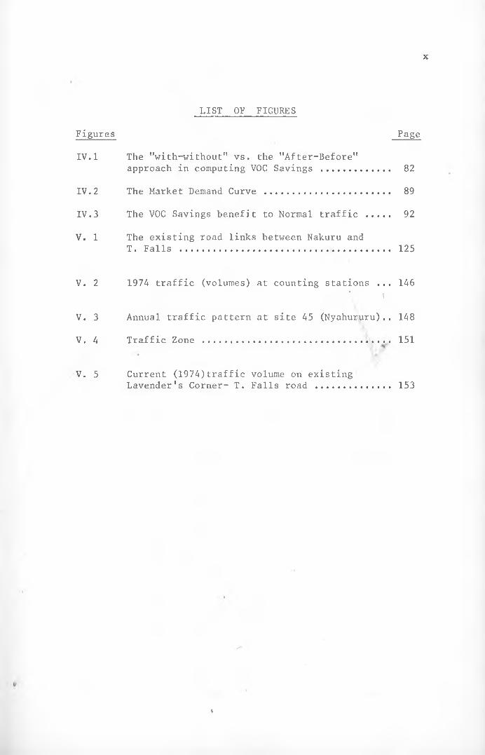
LIST OF FIGURES

Figures Page

IV. 1 The "with-without" vs. the "After-Before" approach in computing VOC Savings ............ 82

IV. 2 The Market Demand Curve ...................... 89

IV. 3 The VOC Savings benefit to Normal traffic .... 92

V. 1 The existing road links between Nakuru and T. Falls ..................................... 125

V. 2 1974 traffic (volumes) at counting stations ... 146' \ ■

V. 3 Annual traffic pattern at site 45 (Nyahururu).. 148

V. 4 Traffic Zone ............................ . 151

V. 5 Current (1974)traffic volume on existing Lavender's Corner- T. Falls road ............. 153

%

P A R T O N E

CHAPTER I

1.1 INTRODUCTORY

Reading some of the literature available on Social

Cost-Benefit Analysis (or CBA in short) one'gets the impression

that this branch of Applied Welfare Economics Ijas attained a

very high level of sophistication in its development. This is

true at least of the theoretical literature. Some rather

complicated treatises have been written on virtually every

aspect of CBA - ranging from the identification of costs and

benefits of projects, measuring (i.e. pricing) them, investment

criteria, the treatment of risk and uncertainty, spillover

effects, etc. To illustrate:

1. Mishan^ias proposed an elaborate scheme for the evaluation of the direct and indirect costs and benefits associated with a project based on what he terms the "willingness-to-pay".

2. Little and Mirrlees2 have also come up with an 'even more complex alternative approach to the evaluation of the cost and benefit items of an investment project.

*E. J. Mishan "Cost-Benefit Analysis ...."

2Little and Mirrlees "Manual of Industrial Project Analysis ...."%

- 2 -

Of all the problems in CBA that of measuring costs and

benefits - both direct and indirect - is the most fundamental.

Yet, apparently it is one area in which not much progress has

been made - not much at least in relation to the advances that

have been made in the other areas of Cost-Benefit Analysis.

For instance, the application of Operations Research techniques,

e.g. Probability Theory, Game and Decision Theory, etc., has

made it possible to grapple with the problems of risk and

uncertainty with a reasonable degree of effectiveness and

confidence. Regression and correlation techniques are now

established tools in forecasting. Refined investment criteria

(or decision rules) such as the now popular Internal Rate of

Return (IRR) or the Net Present Value (NPV) are now common

place, having developed over time from measures such as the

simple rate of return (still widely used in simple financial

analyses) and the pay-back period. The problem of inconsistencies

which used to arise in ranking investments on the basis of the

three decision rules in common use nowadays - namely the IRR,

the NPV and the Benefit-Cost (B/C) Ratio - have virtually been

overcome by the "Normalization Procedure", which Mishan3 has

elaborated very well in his book.

Yet all these refinements are in vain if the raw data

used in cost-benefit calculations are only crude approximations.

Such data are derived by two basic processes:

(1) identifying and enumerating the cost- benefit items.

E. J. Mishan, Op. Cit, Chapters 34-373

- 3 -

(2) measuring these items in money terms.

There is nothing particularly difficult in identifying the costs

or benefits of a public sector project. But two

factors should be borne in mind in doing so:

(a) for CBA purposes all costs and benefits should be social as distinct from private costs and benefits - i.e. they should relate to the whole economy rather than to private individuals or organizations.

(b) costs and benefits fall into two broad categories:

(i) direct (efficiency) costs andbenefits consisting of intended social outlays and anticipated outputs and ; , *-

(ii) secondary or indirect costs and benefits - i.e. the unintended adverse and favourable effects of a project.

The efficiency effects - the flow of intended inputs

and anticipated outputs - are relatively easier to identify

than the indirect ones. The direct inputs for, say the con

struction of a new road or the improvement of an existing one

are the real resources that society must forgo to have the new

or better road. The corresponding benefits will be the gains

that are expected to accrue to road users in particular and to

society at large. Suqh gains will include items as varied in

nature as savings in vehicle operating costs, journey-time,

lower risk of accident or greater comfort and reliability.

Indirect project costs and benefits also take various forms.

The point about them at this stage is that, unlike the direct

effects of a project;, they are the unintended ramifications of

- 4 -

a project and are not as easy to identify. It would appear

from the literature there is no general consensus among CF>A

experts as to how the secondary effects of a project should be

treated. Some analysts advocate they should be excluded from

the costs and benefits of a project altogether. Others feel

this is rather an extreme position and suggest that as far as

is possible, under certain circumstances, secondary project

effects should be taken into account in the evaluation of a

public sector project. Mishan, for example, suggests that

increases in site (property) values should be counted as benefits

if it can be shown that they are not mere transfers of valueA. ( V .

from properties located elsewhere in the economy to properties

situated near or along a road or some other investment. As a

further illustration, the Foreign and Commonwealth Office (FCO)

and the Overseas Development Administration (ODA) in their

"Guide to Project Appraisal in Developing Countries" propose

that "backward linkage" effects of a project be included either

as costs or benefits, as the case may be. However, they caution

against incorporating "multiplier" effects.

Apart from these scattered and brief cautionary remarks

most of the CBA literature tends to shun the treatment of

indirect project effects. The majority of those who prefer that

secondary effects be kept out of the picture altogether do so

on the grounds that they are too difficult to trace and evaluate.

Moreover, even those who advocate a more positive approach also

call for care on the part of the project analyst in his treat

ment of secondary^costs and benefits of a project. At its

5

current stage of development it would appear that CBA is still

ill-equipped to tackle secondary project effects properly; and

in the developing countries where the additional problems of

lack or inadequacy of statistical information and shortages of

properly trained project appraisers abound, it is probably best

only to take note of the possibility or actual existence of these

effects without attempting to trace and evaluate them.

The second fundamental step in the appraisal of a pro-t

ject is how to measure the worth to society of the inputs andt

outputs of the project. Since.both inputs and outputs contain

items of different types there is need to convert them to a

common measure so that a single summary index for the net worth

of the project to society can be derived.

Problems associated with the measurement or evaluation

of project inputs and outputs are even more troublesome than

those of identification. Firstly, the worth of project inputs

and outputs in cost-benefit calculations is social or economic

- not private - worth. The measure of the private worth of a

project's inputs and outputs would be the market prices at which

they sell. On the other hand, market prices are usually poor

indicators of economic value and must be adjusted to reflect

the social valuation of goods and services produced in an

economy. Only if an economy is so competitive that market

prices are determined largely by the interplay of "market forces"

of supply and demand can such prices be regarded as a fair

measure of social value. A major measurement problem then is»

\ - 6 -

one of how to adjust market prices to reflect what is considered

to be the social worth of the goods and services that are the

inputs and outputs of an investment project.

The problem stated in the foregoing paragraph is one of

adjusting already available market prices. A slightly different

but related problem is to establish a price where none exists.

Two aspects of this should be distinguished:

(a) the problem of determining the price of a product that has not been in existence before. To do this it may be helpful to know something about the pricing policy of the producer of the new product. Possible bases for pricing decision^ * are Marginal Cost (MC) and Average Cost (AC). However, the use of these two pricing criteria subsumes:

either (i) that the economy issufficiently competitive to ensure a close correspondence between MC or AC and the market price;

or (ii) that the producer hassufficient influence over his market to enable him to set his price in line with his MC or AC.

In the latter case we are once again confronted with

the problem of having to adjust the market price to arrive at

the social value of-the product in question. In a highly com

petitive economic setting the market price, whether it be

equivalent to MC or AC, would be considered as an acceptable

approximation of the social value of a good or service.

%

7

(b) determining a price for a non-marketable or non-marketed product - e.g. a "public good", a spillover effect, an intangible item such as improvements in the scenery of a locality. Since in the so-called "market economies" a major factor in the determination of value is the interaction of supply and demand, the valuation of goods and services for which no markets exist must necessarily be arbitrary.

It is one of the basic axioms in Economics that all

economic production is geared towards the satisfaction of con

sumers' needs - the consumer is supreme: his needs provide the

motivation for production activity. This axiom applies equally

to production activity in both the private and public sectors

of the economy. Hence in CBA the net social worth of an invest

ment is the net benefit that accrues from it to the consumers

of its output(s), Profits from the sale of a project's output

which accrue to the private investor (indluding profit making

government enterprises) are obviously not a social benefit.

Most public sector investments are not undertaken to yield

business profits as their outputs are not produced for the

market. They do, however, yield benefits to society. The

social worth of both private and public sector projects is

measured in terms of Consumers' Surplus (CS) - i.e. the dif

ference between consumers' maximum willingness-to-pay and what

they actually pay directly or indirectly in terms of forgone

tangible benefits or opportunities.

Basically CS is an economic concept that is virtually

impossible to measure accurately. In economic theory it refers

to the surplus utiiity a consumer enjoys from consuming a good

\ - 8 -

or service but for which he does not pay, although he would

be prepared to pay if he were required to do so. In CBA net

benefit is considered in terms of this amount of money (or some

other valuable asset) that the consumer would be prepared to

pay rather than go without the good or service in question.

Although this overcomes the difficulty of having to convert

CS into its money equivalent, it raise* a new difficulty. To

obtain the monetary CS associated with the consumption of a

given good or service one requires to have a demand curve for

the good or service. But, as any honest economist will admit

one of the most difficult tasks in economics is £o establish

a demand curve for a good with anything like "reasonable

accuracy". By definition a demand curve represents consumers *

purchase plans. To determine a demand curve is to establish

these plans in quantitative terms. This is an exercise that is

replete with all manner of difficulties, not the least of which

is uncertainty about the behaviour of consumers. Commenting on

consumer behaviour at large William Stanton1* makes the following

rather humorous remark which succinctly underlines the causal

influences behind this uncertainty:

"If he (the consumer)is king, he maintains a strange palace court in which the subjects ( sellers) have to spend huge sums to try to find out what the vacillating, disorganized fickle king desires and to proclaim loudly that they, over all courtiers, have just what he wants".

** William J. Stanton, "Fundamentals of Marketing" (1971)page 175.

%

The various techniques that economists and statisticians have

’ developed so far for the purpose of determining and predicting

what the "disorganized, fickle king desires" at best yield only

rough approximations. Among them are consumer surveys, test

markets, market trend analyses which rely heavily on the

regression technique, etc. These techniques can be applied

only to establish the demand for goods that have a market.

For non-marketed products it would not even be appropriate to

talk of them as having demand curves since, strictly, demand

curves represent price-quantity relationships. Public goods,

for example, have no price as such. Yet in CBA it is this type

of product for which one needs to calculate CS to arrive at

their social worth. The social value of marketed or marketable

goods and services is easier to determine because all that is

required is to adjust their market prices so that they reflect

their economic values. For public goods one must establish a

premise for pricing them. The trouble is that one may have no

way of telling whether the premise is correct or not. Con

sequently, there is no clue as to the correctness of the price

one attaches to a public good.

1.2 PURPOSE AND SCOPE OF THE PAPER

This paper attempts to focus attention on the basic

problems involved in appraising road transport projects in

particular and public sector projects in general. The public

sector is a very large portion of the economy in many of the

developing countries in Africa and Asia. In some of them it

comprises virtually^ the entire economy, save for minor

10 -

activities. In the so-called "mixed economies" it may be as

large and as important as the private sector. Notwithstanding

the relative size of the public sector in any one country, the

fact is that its existence and importance must be reckoned with

even in the industrialized, largely market economies of Western

Europe and North America.

It is this fact which gives CBk its present eminence in

government planning agencies in many countries and in academic

circles. As an aid to rational investment decisions in the

public sector, CBA is invaluable. In fact Its very "raison■ V *

d'etre" is to aid the project analyst to deploy a' country's

scarce resources in a manner that yields maximum net benefit

to society. In oth«r words, CBA should be a practical planning

tool. But indications seem to be that while it has made con

siderable advances on the theoretical front, it is still lacking

in a number of aspects in the realm of practice. But in view of

the great need for the application of its principles and techni

ques, it is imperative that, while CBA should certaintly retain

its respectability as an academic discipline, it should be a

practical tool for project planning.

This paper will limit itself to a detailed examination

of the two basic steps in estimating the costs and benefits of

a project which were mentioned earlier - i.e. the identification

and evaluation of the inputs and outputs of a road project. The

actual transportation of people and goods belongs more to the

private sector - at least this is the case in Kenya. The paper

r 11

will also touch on other areas in CBA such as discountings

investment criteria, uncertainty, etc. But their inclusion is

for the sake of completeness and no effort will be made to deal

with them in detail.

The reason for the preoccupation with the two steps in

the estimation process is that they form the foundation on which

work in other areas is built. The ingenuity of the discounting

techniques is meaningless if the streams of costs and benefits

discounted have not been properly determined. Errors in either

identifying the nature and magnitude of the physical inputs and

outputs or in estimating their money values would" render any

subsequent analysis of little value, no matter how sophisticated

the analysis may be. 1

1 • 3 STATEMENT OF HYPOTHESIS

This paper is not the professional treatise of an expert

in cost-benefit analysis: rather it represents the reaction of

a novice in the "business" of project appraisal in the public

sector to the kind of problems that the expert has to grapple

with in his work. It focuses specifically on the conceptual

and practical difficulties that arise in the process of identi

fying and evaluating-project inputs and outputs. Some of the

issues raised in it may be problems for which solutions already

exist but which the writer is unaware of; others may be problems

of his own making possibly because of his own inexperience in

handling them. But whatever the case may be, it appears that,

despite the very commendable contribution theorists have made

12to the growth and development of CBA as a discipline worthy of

academic study, questions of its practical use have not received

as much attention as they should - a failing which has created

a discrepancy between the theoretical and practical aspects of

the subject. And in this gap seems to lie the root cause of the

difficulties that plague the project planner's work in the field.

It is therefore suggested here that the existence of

this discrepancy between the levels of development in the theory

and practice of CBA gives rise to the undesirable consequence

that some of the CBA concepts, so eleborately expounded byV.

theorists cannot easily be translated into usabl<f form. Con

sequently, efforts aimed at narrowing the theory-practice gap

would be far more rewarding than further theoretical advances.

A basic premise taken in this paper is that CBA is primarily a

practical decision tool in the hands of the economic planner.

This is the main reason why it is desirable that the gap mentioned

above be eliminated or at least reduced. The cause of the

discrepancy seems rooted in both the concepts and estimation

procedures proposed by the theorists. Some of the problems

that the planner encounters in practice arise from the difficulty

in measuring some of the concepts he has' to use. But a good

number of his troubles seem to spring from the complexity of the

procedures and models that have been advanced by writers for

purposes of identifying and evaluating project cost-benefit

items. The narrowing of the said gap then must proceed on two

fronts:

- 13 -

(i) redefining unclear or too abstract concepts (or possibly formulating new ones where necessary) in a manner that makes them easily understood and measurable.

(ii) simplifying or reformulatingestimation procedures and models to make it possible for those intended to use them to handle them with ease and confidence.

Generally less difficulty arises in identifying the

(direct) cost and benefit items of a project. The indirect

effects, however, are sometimes obscure. But this is a pro

blem in tracing - not identifying - the effects. The greatest

diffficulties are in trying to measure the value' of project

effects - whether these are direct or indirect. And this is

the reason why a number of alternative approaches have been

proposed by the various "schools of thought" in CBA. The two

prominent such approaches which will be considered in this

paper are:

1. the Willingness-to-pay method - championed by the majority of thinkers and writers on CBA including, among others Mishan, Prest,Turvey, Millward etc. Under this approach the costs and benefits of a project are measured in terms of what people are prepared to pay for them - i.e. measured by the prices they would pay for them.

2. Under the World (Border) Prices approach, first propounded by Ian M. Little and James Mirrlees, project inputs and outputs would be valued at import-export prices.

Both of these evaluation proposals raise both conceptual

and procedural difficulties. Detailed discussion of these is

deferred to later,chapters. Suffice to remark here in general

14 -

that some serious misgivings have been expressed about each of

these two approaches and on CBA as a whole. One of the main

problems in the willingness-to-pay approach is that the domestic

market prices which are taken as the measure of people's

willingness-to-pay do not always reflect the social value of

goods and services. They have to be adjusted to do this - the

adjusted prices being termed "shadow prices". It is in

attempting to determine shadow prices that the planner finds

the greatest valuation problem. To date there seems to be no

set formula for converting market prices into shadow prices.

Loose statements to the effect that the shadow prices of inputs' .1., <

should be the money values of the inputs' opportunity costs do

not appear to be very helpful. The question still remains as

to exactly how the opportunity values of the inputs are to be

determined. The social values of outputs are usually derived

by adjusting market prices for distortions in them due to

indirect taxes and subsidies of various sorts. But then market

prices may fail to reflect social worth properly for reasons

other than fiscal effects, for example monopolistic influences.

No specific direction is available as to how monopolistic dis

tortions may be eliminated from market prices to arrive at a

social measure of goods and services. Economic theory has it

that market prices would be ideal measures of social value in a

perfectly competitive economic setting. The real world economies

are far from being perfectly competitive so that in practice

there is no such standard of judgement against which market

prices may be gauged.%

15 -

In terms of validity willingness-to-pay is a highly

commendable concept. One short-coming of the approach is the

apparent lack of some definite procedural mechanics of deriving

shadow values, given that the market measures of willingness-

to-pay - namely the commodity and factor prices - are not

necessarily appropriate measures of people's valuation.

In the Little-Mirrlees model world prices are regarded

as the direct measures of social worth. The prices of goods

and services on the international market are, therefore, shadow

prices and require no further adjustments. The arguments for

and against this approach have been the subject 0T some con

troversy in the literature and will be discussed in the next

chapter. At this juncture it will only be noted that the

Little-Mirrlees approach as a whole is both controversial

regarding its validity and objectionable on account of its

complexity. Price Gittinger has the following remarks to make

about it:

"Since the appearance of the Little and Mirrlees' second volume in 1969, their valuation proposals have aroused a continuing exchange among planners in developing countries and among professional development economists. Comments about the system have centered around its complexity and whether in fact it leads to better investment decisions.There is little doubt that their system of determining accounting prices is difficult both to understand and to apply.Even highly trained economists admit ambiguities in the system as Little and Mirrlees expound it and question its practical application."5

5J. P. Gittinger, "Economic Analysis of Agricultural Projects"(1972), p.45.

16

When he wrote Gittinger was a division chief .in the World Bank's

Economic Development Institute responsible for its training

program in agricultural project evaluation - a position which

afforded him closer acquaintance with the practical problems in

project analysis than the academic theorists can ever have.

Gittinger, along with many other writers, is not only complaining

that the Little-Mirrlees model is too complicated for most pro

ject appraisers (partly because of the very high degree of

mathematical facility it calls for); he is also questioning

the validity of it as may be deduced from the words:

y.Comments have centered around

whether in fact it leads to better investment decisions".

This criticism may imply one or both of two deficiencies in the

model - namely:

(1) that the computational mechanics of the model is faulty. This would be a problem in the mathematics of it which need not concern us here.

(2) that the logic of the assumptions and other premises underlying it are invalid.If this is so then the above criticism is very much the concern of this paper - and it is an important one.

The view that the Little-Mirrlees system is too complicated is

further borne out by the fact that the Foreign and Commonwealth

Office (FCO) in conjunction with the Overseas Development

Administration (ODA) have found it necessary to write a more

simplified version of the original manual.

%

- 17 -

The FCO/ODA adaptation of the Little-Mirrlees model is

one instance of the reduction in the theory-practice discrepancy

which is being advocated here. When the gap between what is

theoretically plausible and what is practically useful is so

wide as in the case of Little-Mirrlees system it only serves to

frustrate the very people who are expected to translate theory

into practice. This has at least two harmful consequences:

(i) the project appraisals done with the aid of only partially understood concepts and techniques must necessarily be distorted, except if chance and coincidence operate in favour of the appraisers. And, moreover, this is assuming that the appraisers haye the patience and courage to withstand Che psychological discomfort of knowihg that they are working with models that they do not fully comprehend.

(ii) the development of CBA to maturity wouldbe stultified if it cannot find encouragement and nourishment from the experience of practical application. Developing countries, which, it is said, stand to benefit most from the application of CBA have no need for fine ideas or models which cannot be applied easily to solve their myriads of development problems. The saying: "knowledge for its own sake" is very relevant to such things as art and the like and in countries where basic needs are not much of a bother. Technology - and CBA is part of it - is essentially utilitarian: itmust even be more so in the backward regions of the world.

But the problems in the application of CBA such as have

been mentioned above must be seen in the context of the nature

of the subject. One of the fundamental causes of difficulty

in CBA is that it is a social science - and this, among other%

things, implies that the degree of rigor and precision of the

- 18 -

mathematician and the physical scientist are difficult, if not

> impossible, to attain in the analysis and solution of CBA pro

blems. Those who complain about the lack of these qualities

and the range of assumptions in cost-benefit studies display

a failure to realize this fundamental point. The lack of

mathematical rigor and precision in the social sciences is deeply

rooted in their psycho-social nature. Underlying the data and

method of analysis, interpretation and predictions of the

social scientist is human behaviour which is as difficult to

comprehend fully and to manipulate as it is infinitely varied.

There are not as many constant "laws" in the realm of psycho-y*.

social behaviour as there are in the physical world - a point

which largely absolves the social scientist from the indictment

of imprecision and lack of rigor. But this must not be taken

as an excuse for the social scientist to be unnecessarily care

less in the formulation of his concepts or analytical procedures.

It simply means that a certain amount of imprecision must be

tolerated in the social sciences. In some areas the cost-

benefit analyst, for example, may not even be able to quantify

some of the variables he manipulates. Asked how far he thought

CBA could be applied in appraising educational projects such as

the MBA degree program recently introduced at the University of

Nairobi a C.I.D.A. official retorted:

"I have given up ever trying to apply CBA to education, health or any other social service ....".

This may be unwarranted despair on the part of the official but

it does illustrate that there are legitimate limitations to be

- 19 -

reckoned with in the social sciences. Fortunately cost-benefit

analysts and general economists have never pretended that it is

an easy matter to appraise "social service" projects. The

problems which bedevil any quantitative appraisal of the net

worth of such projects are well known and fully acknowledged.

1.4 METHODOLOGY

The method adopted in this paper to illustrate the gap

between theory and practice in CBA consists simply of a comparison

of the theoretical and practical aspects of project appraisal.y»

To this end a statement of the theoretical aspect will first be

presented, followed by a case study of a proposed road project

in Kenya's Rift Valley Province. The reason for juxtaposing

these two is to Highlight the extent to which current practice

falls short of the theory. To be sure some of the short-comings

in the application of the principles will be due to short

comings in the empirical data of the case study. Where this is

so it will be pointed out. But this type of difficulty is not

the principal concern of this paper, although obviously

empirical problems are important. The short-comings in the

piece of research done for the case study will undoubtedly have

some bearing on the 'conclusions to be drawn from the case study

regarding the theory-practice discrepancy. The main interest►

of the paper, however, centers on those problems which would

still arise even with the most well planned and conducted data

gathering and analysis. Difficulties which arise out of the

writer's faults in the collection and processing of the field

20 -data will be indicated wherever possible and they should be

regarded as being peripheral to the theme of this thesis. Dis

crepancies between a principle and its application may arise

possibly because of the misconception of it on the part of the

person who makes use of it. This would be a grievous fault and

it is hoped that the possibility of occurrence of such a mistake

in this paper is remote.

In the following chapters are set out details of the

theoretical framework which in a way forms the back-bone of the

thesis. This description is preceded by some introductoryi.

remarks on the peculiar characteristics of appraisal problems

in the transport sector, followed by a detailed consideration

of the enumeration and evaluation of inputs and outputs of a

road project. The theoretical framework sets out the analytical

procedures to be followed in the case study.

The case study will be presented in three sections dealing

with a general description of the case study of the road project

and its area of influence, the data gathering process and the

presentation and analysis of the field data. The role of the

case study must be seen as being purely instrumental in justifying

(or disproving) the hypothesis posed earlier.

It will probably be difficult to find inadequacies in

the empirical data which are not in one sense or another associa

ted with the way the concepts of cost and benefit are defined.

It is this association which prompted the hypothesis that the

major evaluation problems are rooted in the theoretical aspect

of Cost-Benefit Analysis.

P A R T T W O

THE THEORETICAL FRAMEWORK

CHAPTER II

TRANSPORT SECTOR PROJECTS

2 . 1 general

In East Africa most of the transport sector of the

economy is under some form or other of government ownership or1 •• , , 1 V ,control. Railway, lake steamer; harbor facilities; internal

and international air services are all operated by East African

Community corporations - namely the East African Railways

Corporation (EARC), the East African Harbors Corporation (EAHC),

and the East African Airways Corporation (EAAC). These cor

porations are jointly and wholly owned by the three partner

governments of Kenya, Tanzania and Uganda. Some lake and

internal charter flights are operated by small private firms

but these are an insignificant proportion of the total volume

of inland and sea and internal air transport services in East

Africa. Railway services are the exclusive monopoly of the

EARC.

Road transport is the only one in which the private

sector may have a significant share. However, even this is

probably true only in Kenya, and possibly, Uganda. In her

nationalization moves, socialist Tanzania brought all major

22companies operating within her territory under public or govern

ment ownership. With the exception of small local services,

road transport is virtually wholly a public sector service in

Tanzania. In Kenya and Uganda the Governments limit their role

in the field of road transport to the construction and maintenance

of roads. Operating road transport services is left open to

the private sector. Only in one instc.ice is the Kenya Government

known to have extended its interest to actually operating road

transport services: through KENATCO the Government participates

in heavy road haulage and taxi hire service. The only one of

the local authorities in the country having a hand in road

transport is the City Council of Nairobi with a .minority share/

interest in the Kenya Bus Services company - a public service

company operating in Nairobi and Mombasa.

Currently plans are underway to build an oil pipeline

from the oil refinery at Mombasa to Nairobi and possibly to be

extended to Kampala (Uganda) in future. Indications are that

this project might be undertaken jointly by the Governments

of the two countries, perhaps in conjunction with some minority

interest private shareholder(s) in the proposed pipeline company.

If the project does materialize, East Africa will have added to

its transport system a dimension that has so far only been

limited to bringing water to urban areas from local dams.

Given the highland nature of the East African topography

and the small size of the region's rivers, it is unlikely that

rivers or canals will ever become an important part of the

- 23 -

transport system in this part of the world.

2.2 TYPES OF TRANSPORT PROJECTS

The foregoing description gives some indication of the

type of projects that could be undertaken by the government or

some agency acting on its behalf - i.e. projects which call for

Cost-Benefit appraisal. Such projects would include:

Road Transport

(i) Construction of a new major or minor road.

(ii) Improving or reconstructing an existing trunk or feeder road.

(iii) Construction of a set of special purpose roads: tea roads, sugar roads, tourist roads, etc.

Railway Transport:

(i) Building a new railway line or extending an existing one: forsome time now the EARC has been persistently urged to extend the Kisumu-Butere line to link up with the main Nairobi-Kampala at Bungoma to serve the agriculturally vital Western Province. Another possibility which has also been mentioned is the extension of the Nakuru-Kisumu line to Kisii and possibly to Homa Bay on Lake Victoria to help opening up the claimed potential copper deposits in South Nyanza and to serve the coffee-rich Kisii highlands.

(ii) Purchasing new locomotives: thusas part of its modernization program the EARC recently purchased some ninety diesel-electric engines to replace its now outmoded diesel engines.

24 -

(iii) Increasing,"rolling-stock"; the EARC has recently come under pressure to increase its carrying capacity, particularly at harvest time when farmers' storage capacity is exhausted.

(iv) Increasing or modernizing passenger coaches or building some other facility.

Air and Sea Transport

(i) Construction of an airport or harbor

(ii) Purchasing a fleet of aircract or ships: there are plans afoot to replace the present fl EAAC's fleet of VC10 jets with DC9 aircraft. ' , v

(iii) Opening new internal or international flight services.

Each one of the community corporations which would

undertake the above projects operates on a commercial basis:

it is expected to make profits like any other commercial

enterprise. For this reason a profitability analysis of the

projects would be a first and necessary step. But to the extent

that the projects would be financed by public funds, cost-

benefit appraisals of the projects would not be out of place.

Although the projects would primarily be commercial undertakings,

they must also be seen as economic enterprises the social

profitability of which must be established. Ideally then any

of the above projects would have to satisfy both commercial and

social profitability requirements to qualify for undertaking.

In many cases a commercially profitable investment may also be%

- 25 -economically viable. But there may well be projects which

may be commercially sound but economically undesirable. These

are the projects that pose the greatest evaluation problems.

Whether they are undertaken or not will depend largely on what

policy guidelines the government may have laid down affecting

investment decisions. But in the absence of this, given that

the Community corporations are firstly commercial enterprises

and only secondly "socioeconomic" institutions, private profit

ability considerations may take precedence over social

considerations.

As experience in Kenya and Uganda has pbfown the private

sector in any one of the East African countries would be quite

capable of providing efficient and adequate road passenger and

freight transportation if public authorities provide the

necessary infrastructure. The Tanzanian nationalization of bus

and road transport companies appears to have been prompted by

political-ideological rather than economic considerations of

efficiency or effectiveness. On the face of it the small scale

nature of the road transport business would seem to favour

private operations. Public ownership and operation would be more

suited for such large-scale undertakings as rail or air services.

These require substantially heavier initial investment outlays

than most private firms in East Africa would be ready to

undertake.

%

26 -

2*3 IDENTIFYING PROJECT COSTS AND BENEFITS

To calculate the net commercial or social profitability

of an investment project two sets of basic data are required:

quantities of the physical inputs and outputs and prices at

which these are to be valued. For meaningful comparison of the

various types of input items on the one hand and output items

on the other it is necessary that they be converted to some common

measure - the usual and obvious one being money. There are then,

two distinct but related basic steps in the appraisal of a

project:I

1. identifying (or enumerating) ancj quantifyingthe physical inputs to be used up by a project and the physical outputs it is expected to produce. v

2. determining the monetary prices at which to value the inputs and outputs.

Both of these steps are by no means easy but generally it is

easier to identify and quantify a project's inputs than its

outputs. Every project uses up real (economic) resources in the

form of time, effort and materials and these are not too

difficult to identify or to quantify. The outputs of some pro

jects, though economic in nature, are intangible and not easily

recognizable as benefits, e.g. the comfort road users enjoy

driving on a smooth surfaced road; others may be both intangible

and non-economic - e.g. the prestige (real or imagined) to a

country from having a monumental building, stadium or some other

imposing structure or the aesthetic value of a public park, etc.

When the benefits expected from a project are largely or wholly

non-economic in nature so that an economic valuation of them is

not possible, economists do caution investment decision makers

- i n

t o bear in mind that tie resources that such a project absorbs

are a real cost to the economy.

Secondly, there is the element of uncertainty to reckon

with in quantifying project inputs and outputs: one can never

be certain about the exact amount of resources a proposed

project will use up or the precise magnitude of output(s) it

will produce. This problem is of particular significance in

relation to operating cost and benefit items the flow of which

stretches further into the future. The degree of uncertainty

increases the further into the future one projects so thati.• . , •forecasts of the magnitudes of cost/benefit items that will be

realized in the relatively more distant future are less reliable

than forecasts about the near future.

2.31 'ENUMERATING PROJECT COSTS

The economic costs associated with a road project fall

into three broad categories:

(a) Construction costs

(b) Maintenance costs

(c) Incidental adverse effects or externalities resulting from the construction and utilization of the road affecting the road users themselves and/or the inhabitants of the area it traverses.

(a) Construction Costs

These are generally the largest cost item for a road

project. They can be sub-divided into:

(i) Cost of capital goods - construction equipment like bull-dozers, scrappers, rollers, motor-graders, tippers, etc.

28 -

(ii) Cost of construction materials - stone aggregate and c'nippings, cement, bitumen, etc.

(iii) Cost of fuel and lubricants

(iv) Land acquisition costs

(v) Cost of labor - skilled and unskilled.

(b) Maintenance Costs

These are the recurrent costs of keeping a road in

usable condition. With the exception of such things as land,

maintenance costs will consist much of the same items as con

struction costs. How often these costs are incurred - hence

their magnitude - will, among other things, depend on the

standard of construction adopted. This also determines when

they start to be incurred after construction.

Note: Contingency Allowances

Estimates of construction and maintenance costs are

liable to some margin of error. There are two sources of error

for which allowance should be made. First there may be errors

in estimating the quantities of physical inputs. Provision

should be made for the possibility of increases in the quantities

of the inputs required for construction and maintenance. The

second source of error is in pricing the inputs: provision

should be made in the cost estimates for possible increases in

the prices of such items as materials, fuel and labour. If,

however, prices are expected to change in such a way that the

input relative prices remain unchanged or if the road project

costs (and benefits) are valued in real terms this second

provision should qot be made. If input relative prices remain

29 -

unchanged total construction and maintenance costs will be

unaffected by changes in the prices of individual input items

because the price movements will neutralize one another. If

the costs are measured at constant prices, moreover, current

or future prices are rendered irrelevant in the valuation of

project inputs.

(c) Adverse Spillover Effects

If a project gives rise to incidental effects which

affect society adversely they should, as far as is possible, be

evaluated and added to the intended money cost$ or alternatively

subtracted from the benefits of the project. Common adverseV.. . . '’A, *spillover effects associated with road projects may be:

(i) pollution of the environment - largely in the form of smoke and noise from passing vehicles

(ii) traffic congestion: if the constructionor reconstruction of a road generates more traffic volume than it was designed to carry, those who travel on it (in their own vehicles) will incur extra journey costs in terms of increased fuel consumption, delays and annoyance.Although incidental, these effects are real social costs.

2.32 ENUMERATING PROJECT BENEFITS

Categories of Traffic:

The benefits of, a road accrue directly to those who use

it and, perhaps, only indirectly to the rest of society. The

direct beneficiaries may be those who actually travel on the

road or those who transport goods on it. The transportation

of people and the conveyance of goods on a road constitute the

traffic for the road.% In order to identify the direct benefits

from a road economists find it convenient to classify the

\ - 30 -

the traffic on it into the following categories:

(a) Normal Traffic

Consists of those who would use an existing road

regardless of whether it is improved or not. In the majority

of cases road projects involve the upgrading of an already

existing road or the construction of a new road to replace an

existing one. It is rare that a road is built into an area

where there has not been some route, even if it is only a

footpath. In this essay the term "road project" is taken to

mean either of the above two undertakings.v INormal traffic then is the traffic that would continue

to use an existing road whether it is improved (upgraded or

replaced by a new one) or not.

(b) Generated Traffic

This is entirely new traffic which would not come into

existence if an existing road is not improved. It may consist

of one or both of the following:

(i) extra journeys undertaken by the present users of the existing road solely as a result of the road having been improved. This should, however, be carefully distinguished from the extra journeys that would be undertaken as a result of growth in normal traffic;

(ii) extra journeys made by new road users who would otherwise not have utilized the existing road if it were not improved.

Generated traffic reflects the increase in economic

31

activity stimulated by the construction or improvement of a

road in the area of its influence. On the other hand, an

increase in normal traffic, although it does also reflect

increased economic activity, cannot be attributed to the

road improvement because, by definition, such normal traffic

growth would have occurred with or without the improvement.

(c) Diverted Traffic

Consists of those who, in the absence of the planned

improvement of an existing road, would travel by other roads

or use some other different mode(s) of transport.. They are

attracted to use the new road in the hope of deriving some

benefit by so doing.

Benefit items;

In East Africa the services of road facilities are in

the category of "public goods" - goods the amount of which

consumed by any one individual is also the amount consumed by

all its users. There is thus no way of determining how much

of such a good each person consumes so that there is no way of

deciding what price to charge for it. Consequently, a public

good has no market in the commercial sense. This special

characteristic of public goods largely explains why they are

usually provided by public authorities even in strongly market-

oriented economies. The market mechanism depends crucially on

the existence of a price for any good that is or can be marketed.

But for a good to have a price it must be possible to determine

how much of it a person or group of persons consume at any given time

- 3 2 -

Ultimately the benefit the consumers of a good or

service derive from consuming it is the satisfaction or utility

they enjoy. But utility is an abstract concept which is

difficult to measure and apply in empirical studies. The con

cept, mentioned earlier, which project analysts employ,in

practice is that of willingness—to—pay which is not only easier

to measure but also has the further property of being an

indicator of the strength of the desire of consumers for a good

or service. Traditional economic theory defines utility as a

state of being content. The sources of utility may be physical,

social or even spiritual but the notion refers to a purely

psychic property. The trouble with it is that it i's also used

in senses other than the psychological one in which economists

use it. For example, many students being introduced to economics

for the first time find it difficult to avoid conceiving of

utility as some biological satiation especially when it is so

closely associated with almost equally ambiguous terms like the

"consumer", "goods", etc.

Moreover, for analytical purposes the term utility is

inferior to the willingness-to-pay concept in that the associa

tion between the latter term and its empirical measure - money

prices - is evident even’to the non-economist. On the other

hand, one of the greatest difficulties in elementary economics

is for beginners to visualize the. connection between the price

a person pays for an item and the utility he anticipates to

derive from it. And herein lies the root cause of the confusion

that bedevils the "cardinal" approach in the study of consumer

- 33 -

behaviour that the price a consumer pays for a good is the money

measure of the "marginal significance" of the good to him. The

willingness-to-pay concept, because of its direct and explicit

association with prices, is more easily acceptable as a measure,

by proxy, of the benefit for which the consumer is prepared to

part with in terms of money or some other valuable item in

exchange. Whether that benefit is termed utility or given some

other appelation is of little consequence and saves us from

having to make the rather awkward assumptipn, so common in

elementary economic text-books, that utility can be measured in

-some fictitious units (such as "utils" and what have you) as

writers are often forced to do in an effort to ’explain the

connection between utility and price. Using the willingness-

to-pay notion, all that is necessary to remember is that willing

ness-to-pay is a measure of the desire that underlies the

decision by a person to pay a specified price for an item. It

is not necessary to know the nature of that desire. All that

one requires to know is its strength since it is this that

determines the price paid. A distinct advantage of the willing-

ness-to-pay is that it is easier to understand, define and

determine a measure for it.

The benefits .that road users derive from a new or

improved road are mostly in the nature of savings - that is,

avoided sacrifices which road users would have incurred if the

road in question were not constructed. Admittedly those who travel

(or transport goods) on the new road would derive some utility

from the fact that ,they incur less cost than they would on the

- 34 -

old road but for purposes of Cost-Benefit analysis it is not the

utility that is of immediate concern. Of direct interest to

the project analyst is the total willingness-to-pay of the

prospective road users for the benefit of having a better road

- this total willingness-to-pay being measured as the sum total

of the costs (sacrifices) they would incur to utilize it. The

purpose of improving an existing road (or any transport facility

is to lessen this sacrifice. The benefit to the road user then

is the difference in the amount of cost users incur in utilizing

a road in its present state and the cost they would incur if it

were improved. Thus the benefit is a saving.

The cost road users incur by travelling or transporting

goods on a road measures the price they are prepared to pay

for the use of that road. If it were possible to express this

price on a unit basis (as "so much per unit of road service")

a relationship between the different levels of this price and

the different "amounts of road service" in the nature of a

demand curve could be derived and the determination of the net

benefit to the road users would be in the form of the conventional

analysis of consumer behaviour. In effect this is what cost-

benefit analysts attempt to do. Just as a decrease in the price

of a marketed product confers a benefit to consumers in the

form of a saving in the price they have to pay; the reduction

in some or all of the total price of utilizing a road is a boon

to the users of the road. However, it should be borne in mind

that not every benefit item associated with a road project need

be a saving. An outline*of the various benefit items is given

- 35 -

in the following paragraphs: it will be noted that, although

the majority of them are "savings", some are not.

The principal benefits are:

(a) Vehicle Operating Cost Savings

Vehicle operating cost (VOC)(or user-cost) savings con

sist of the difference between the costs of running a vehicle

on a poor quality road and the costs of operating it on a new

or improved road. User-cost savings may also be "alternative

cost" savings - i.e. the savings in the costs of travelling

or transporting goods by road and the costs of doing so by some•y\

other mode of transportation. For instance the Alternative

cost saving benefit of the proposed pipeline linking Mombasa

and Nairobi would be the difference between the costs of trans

porting petrol by road in tankers and the operating costs of

pipeline transmission.

Specific operating cost items in which savings might

be realized would be:

(i) fuel and lubricants

(ii) vehicle tyres

(iii) vehicle (or pipeline) maintenance

(b) Time Savings

There are two main time savings items - namely:

(i) savings in working time

(ii) savings in leisure time

This is a benefit common to all transport projects which make%

the movement of people and goods easier and faster.

36

(c) Savings in (road) Maintenance Costs

An important benefit associated with building a better

quality road or some other transport facility to replace a

similar or different existing one is the possible reduction in

the costs of maintaining the facility to be replaced. If for

instance the proposed Mombasa-Nairobi pipeline does materialize '

it will save the Kenya Government considerable sums of money

currently being spent on keeping the Mombasa road in good

working order. The pipeline would remove a substantial fraction

of the heavy petrol tanker traffic which possibly accounts for

a good amount of damage to the road. v j. •<

/

(d) Reduced Risk of Accidents

In principle, building a wide, smooth surfaced road

should not only reduce journey time to road users but, by

reducing traffic congestion and eliminating concealed corners

and narrow bridges it should also reduce the risk of accidents.

There are two main types of road accidents which may be avoided

by the improvement of a road:

(i) damage to property - vehicles, crops, fences, livestock, etc.

(ii) injury to, or loss of, human life.

But whether building better roads does reduce accident risks is

not an altogether indisputable fact. Experience on Kenya's

paved roads has been one of soaring - not declining - accident

rates. Relatively straight, wide, smooth surface roads seem

to encourage overspeeding and inattentiveness on the part of

- 37 -

drivers which in turn can only enhance the risk of accident.

By no means are these the only causal factors underlying the

rising number of injuries, death tolls and property damage

arising from road accidents. But they seem to be important

contributors. The claimed possible reduction in potential

accidents then is very much contingent upon the assumption that

a good road is in itself an insurance against a rise in the

rate of accidents, which is not true.

(e) Economic Development

This benefit consists of the increase in the output of. . . .such economic activities as agriculture, manufacturing, mining,

tourism, etc. But it is not an easy benefit to identify. As

Hans Adler6, a prominent transport economist with the World

Bank, has pointed out for a road project to be credited with

an increase in economic activity some three conditions must be

satisfied- viz:

(i) That the construction or improvement of the road is the "sine qua non" for such an increase - i.e. that the development would not have occurred without the road improvement.

(ii) That the resources used in the road construction would otherwise have remained underemployed or would have remained idle.

(iii) That the economic activity oractivities stimulated by the road project do not replace other equally or more socially beneficial activities that would otherwise have been undertaken.

6Hans Adler, pp. 2 9 ~ 3 2

- 38

Given these requirements there are some three circumstances

under which a road project may be associated with an increase in

economic development:

1. The road may be an integral part of an agricultural, industrial or tourist project. Investment in the road is, in this case, part and parcel of the investment in the principal project and it would be both impracticable and improper to attempt to show the development effects of the road separately

2. Whether a road is the only bottle-neck to increased economic production - all other requirements, for example, productive facilities readily accessible markets, etc. already exist - the benefits attributable to the road project would be the net increase in the output of the various activities.

3. Where a road is built into an area with considevable development potential the realization of which requires other investments besides the road no particular difficulty arises since, evidently, the road by itself would not generate any development activity.

Thus only if we are faced with the situation described

in (2) above need we worry about tracing the development

effects of a road project.

(f) Comfort and Reliability

Like the "economic development" benefit, these two are

"non-savings" benefits; they are intangible but real. Reliability

in this context refers to the greater likelihood of one success

fully completing a journey or getting goods to intended destina

tions in time on account of a road being in good condition

(and there being enough vehicles on it for road users who do not

- 39 -

own vehicles).

Both benefits are difficult to measure on account of

their being difficult to quantify. It may suffice merely to

recognize their possible existence.

2. 4 MEASURING PROJECT COSTS AND BENEFITS

Two possible approaches to the valuation of the inputs

and outputs of projects were given earlier on as the Willingness-

to-pay and the World (Border) Prices methods. Problems of

measuring project costs and benefits will always arise' V . *

irrespective of which one of these two approaches is adopted./

To emphasize this fact a brief statement of the latter approach

will be given. In general, it is easier to apply than the.

Willingness-to-pay approach but then transport projects pose

special problems which render world prices inappropriate

measures of the costs and benefits.

2.41 VALUATION AT WORLD PRICES

The main reason which prompted Little and Mirrlees to

adopt international instead of domestic prices for the measure

ment of the costs and benefits of projects in developing

countries are the distortions in market prices in these

countries. The system was proposed primarily for industrial

projects but the authors suggest it may be used to value the

inputs and outputs of any other types of projects.

For any one country "world prices" are those it would

40 -

pay for its imports and those it would receive for its exports.

Following is a description of the procedure for determining

"Border Prices". A basic step in the procedure is to classify

project inputs and outputs into "Traded and Non-Traded" goods

(and services). Traded items are those which are or could be

traded on the world market. Non-traded items are those that

do not normally enter world trade and consequently have no

world price.

1. Valuing Costs

(a) Traded Items:

These include categories of input items s«ch as con

struction equipment, materials, fuel and skilled

labour. These may be direct imports or they may be

import substitutes. They should be valued at their

c.i.f. import prices (Pm) or at their Marginal

Import Cost (MIC) depending on whether the market(s)

in which they are traded are reasonably competitive

or not.

Although strictly speaking skilled labour is not

normally traded, for most developing countries it is

an import item and should be valued at its direct

foreign exchange (FE) cost. Even if it is procured

locally it most probably has a FE content (through the

educational and training processes) and should be

valued at the FE equivalent of its domestic cost.

%

- 41 -(b) Non-Traded Items:

A large number of inputs for road projects in developing

countries are traded goods and services. But certain

others like domestic transport, unskilled labour and

some materials (like stone) are not. Little and Mirrlees

suggest the FE values of these items can be obtained

by converting their domestic currency values to FE

values by means of predetermined conversion factors -

computed by a governmental central planning agency.

Unskilled labour, probably the largest non-traded input

especially for projects employing labour-intensive

construction methods, also poses the most troublesome

valuation problems. Firstly it is necessary to

determine its opportunity cost in domestic currency and

then to establish the appropriate conversion factor

for transforming this value to FE.

In the Little-Mirrlees model the SOC of unskilled labour

is to a very large degree influenced by the attitude of

the government (as embodied in its economic policy)

towards saving and consumption in general. If

current consumption is thought to be more important

relative to savings, the social cost of the unskilled

labour employed on a project is considered to be, in

principle, the output forgone in the next best alterna

tive use for the labour. In practice this cost would

simply be the output that the labour would have pro

duced in the sector from which it is drawn to work on

- 42 -

the road project. If a higher premium is placed on

savings - and hence on future consumption - than on

current consumption, the level of the shadow wage rate

will depend on whether the consumption per capita of

those employed on the project out of their wages is

higher or lower than what they were consuming before.

If it is equal to or less than their previous level

of consumption per head the shadow wage will be equiva

lent to the value of the output lost elsewhere by trans-»

ferring the workers to the road project. But if it is

higher the social cost of the unskilled labour will

exceed the value of output forgone elsewhere by the

difference between the previous and current per capita

consumption levels.

2. Valuing Benefits

(a) Traded Output Items:

If the output(s) of a project are or can be exported

they should be valued at their f.o.b. export prices if

the export market is highly competitive. In that case

the export price (Px) for each export item would tend

to be fairly constant and independent of the quantity

(Qx) of it exported. If the export market is not very

competitive the item should be valued at its Marginal

Export Revenue (MER) since in this case Px falls as

Qx increases and vice versa. The net addition to total

export revenue would be MER, not Px.%

- 43 -

If the project's output replaces an import, its

benefit would be the FE saved by not having to import.

Such an import substitute would be valued at the c.i.f.

price, Pm, of the displaced import in case the import

market is competitive. If it is not, then the import

substitute should be valued at the MIC of the replaced

import since under non-perfectly competitve circumstances

Pm would tend to understate the true cost of the item

to the importing country.

In either of these two cases there will be domestic

costs of transport, insurance, and distribution for an

imported good and costs of transport and insurance for

an export. These may be termed respectively as:

(i) port-to-user costs, and

(ii) producer-to-port costs.

For an import substitute the port-to-user costs become

a cost saving when the imported good is replaced. This

cost saving should be converted to its FE equivalent

and added to the FE saving by not importing. For an

exported item the producer-to-port costs would be

converted from its FE earnings.

(b) Non-Traded Goods:

If the output of a project is non~traded its value at

domestic prices should be transformed into FE by means

of a suitable conversion factor for the particular

item(s) or fo r the industry producing it. Non-traded

items include services-like domestic freight, construction

44 -

or electricity. There is no world market for these.

The central point in the Little-Mirrlees approach is

import/export. prices are a better measure of social value than

domestic prices in developing countries, assuming that these

countries adopt the "proper" economic and commercial policies.

There are two basic premises for this contention:

(i) Firstly, whatever distortions there may be in world trade - and hence in import/ export prices - are not peculiar to any one individual country. They affect all countries participating in international trade and are, therefore, irrelevant to valuation problems from the point of view of any given country.

' <•! *(ii) Secondly, fast economic growth and development

which developing countries are so despa- rately in need of depend to a significant degree upon the availability of foreign exchange. Because of its relative scarcity FE is thought to be a more sensitive measure of the social worth of goods and services in developing countries.

Little and Mirrlees advance the following three reasons,

among others, for discrediting domestic market prices as good

measures of social value:

(1) Most developing countries - for example in Latin America - are afflicted with chronic inflation which possibly is symptomatic of imbalances between aggregate demand and supply.

(2) These countries suffer from perenial high levels of unemployment - especially of unskilled labour.This, coupled with government intervention in the labour market (e.g. minimum wage legislation) and other labour market imperfections, result in market wage rates that bear little or no relation to the economic value of the various labour categories.

" 45 “(3) Most developing countries' currencies

are over-valued - i.e. the exchange rates for the currencies are kept artificially at levels much higher than they really need be. Under a regime of freely determined rates the exchange rates would be so low that most developing countries would be beset with even greater balance of payments problems than they are atpresent. This over-valuation is sustained through various measures (exchange control, tariffs, quotas, etc.) devised to protect domestic agriculture, industry and other sectors.

On the face of it, it would appear as if the implication

is that Little and Mirrlees recommend world prices because they

are deemed to be distortion-free. But some supporter^ <£f the

approach argue that the real justification is that whatever

distortions there may be in import-export prices are a common

factor to all countries which buy and sell on the world market.

World prices may, therefore, be taken as a norm or price

standard. On the other hand, domestic price distortions are

peculiar to those countries in which they occur and represent

a departure from the world price standard. What the proponents

of this view-point do not make clear is whether it is to be

understood that the distortions in world prices are considered

irrelevant to valuation problems in any one country because

they affect all countries to the same degree. Clearly, if

this is not the case then indeed the price distortions may not

be irrelevant to some individual countries.

More often some writers have given the impression that

prices in developing countries are considered "distorted"

- 46 -

vis-a-vis prices in developed countries. It is argued that.:

(i) the developed economies are competitiveto a degree that makes the market the major determinant of resource prices. The infuence of non-market forces is a relatively minor factor.

(ii) these economies have attained very high levels of employment - in some cases approaching full employment - so that resource market prices are fairly good measures of resource opportunity values.

(iii) investment projects undertaken indeveloped economies have only marginal influence on the economies in terms of their effects on prices and outputs.Some kinds of projects in developing economies are so large that they have a greater than marginal effect On the economy. Such projects as mulrepurpose dams, large-scale industrial, agricultural or mining projects have been cited as undertakings which might upset existing relative factor or commodity prices because of the sheer magnitude of the resources they absorb and the outputs they produce.

However, whether market prices measure social worth

better in industrial countries than they do in developing

countries, and for whatever reasons this may or may not be

true, seems to be an irrelevant argument. There is clearly

a difference between market prices in developed countries being

good measures of social value in those countries and the same

prices serving as international norms. In the first place, the

prices that rule in each developed country are not necessarily

the prices at which the country buys from or sells on the world

market. They must, therefore, be regarded simply as being

peculiar to the country in which they prevail. Secondly, it

is by no means true that market prices in developed countries

47 -are so free of distortions as some xsnriters have attempted to

show. In this respect the difference between developed and

developing economies is the type and degree of distorting

influences that exist in each of the two types of economy - not

that the one is free of such influences whereas the other is

replete with them.

Moreover, the prices ruling or the world market are

different from those that prevail on the domestic markets in»

the advanced as well as in the developing countries. The

economic and political forces that determine international

prices are not identical to those that operate at home in either

developed or developing countries, although, undoubtedly, the

domestic production and market forces have a bearing on world

market prices. It would, therefore, be misleading for some

people to suggest that domestic prices in developing countries

are a poorer measure of social worth than domestic prices in

developed economies on the grounds that the latter economies

fulfill certain conditions which the former do not. The com

parison is not between market prices in developed and developing

countries but between market prices in any one country vis-a-

vis those ruling on the world market. It is an irrelevant

matter, therefore, whether developed economies are more compe

titive, enjoy higher levels of employment, suffer less from

inflation, are better in this or that respect than developing

economies as far as the pricing of project inputs/outputs at

world prices is concerned.

%

\ - 48It was hinted above that unless it can be shown that

world price distortions affect all countries participants in

world trade in the same way and to the same degree - and to be

sure they do not - they may not altogether be irrelevant con

siderations in project evaluation as Little and Mirrlees and

their supporters would have us believe. If this condition is

not met, the distortions cease to be a common feature to all

the participants. In other words, world prices cease to be an

international price norm.

But even if world prices were acceptable on this score,

they still might not be good enough for the eyaLuation of road

project outputs. No difficulty would arise in using them to

evaluate the inputs. Most construction input items - equipment,

a large number of materials, technical and supervisory personnel

are imported and can easily be valued in terms of import-export

prices. Of the benfit items, VOC savings and maintenance cost

savings car also easily be measured in FE. But it would be

difficult to measure the value of time savings, favourable

spillover effects and comfort in FE. There is firstly the

problem of establishing appropriate values for these items at

domestic prices and, secondly, of converting the values to

their FE equivalent pleasures. The same difficulty would be

encountered in evaluating unskilled labour. This is a general

problem pertaining to all non-traded items.

Some writers have suggested that time savings may not

be an important benefit in developing countries because time%

49- -

in these countries is not a scarce resource as is evidenced by

’ the generally high levels of unemployment. One simple way out

of the problem of evaluating time savings, they suggest, would

be simply to ignore them. The validity of this argument is

questionable. It may be true that for some categories of people

time is not a scarce resource - and it would be desirable to

identify such groups. Moreover, even if it were a general truth

that people in developing countries have plenty of time at their

disposal, it would still be necessary to find a way of measuring

the value of time savings for projects in developed countries

where time is a scarce resource. Like all other non-traded items,.' i . v

time savings raise the two valuation problems mentioned in the

previous paragraph.

Some of those benefits which may seem amenable to FE

valuation may in fact not be so. Induced economic production,

for example, is a generic term embracing goods and services which

can as well as those which cannot appropriately be valued in FE.

The value of agricultural, industrial or minimg outputs for

instance can quite easily be measured in FE since most of the

outputs are or can be traded on the world market. Hut the FE

value of increases in, say, domestic transportation, distribution

services, etc. cannot so easily be determined since these are

non-traded items.

Finally, there are those benefits like comfort the value

of which cannot just be measured. The best one can do is simply

to recognize them.%

- 50 -

Evidently, it would be most illogical and inconsistent

to measure some costs and benefits of a project at world prices

and others at domestic prices. Similarly it would not do to

measure the costs and benefits of some projects in FE and to

measure the costs and benefits of other projects at domestic

prices.

The foregoing problems relate to the validity of the

Little-Mirrlees method. There are also procedural and statistical

difficulties such as:

1. compiling Pm and Px or computing MIC andMER for valuing the inputs and outputs of a project. ^

2. determining the social opportunity costs of input items such as accounting prices for materials or shadow wage rates for labour. An important aspect of this problem is the determination of proper conversion factors for non-traded items. Little and Mirrlees suggest such factors should be prepared by some central planning agency. But it is not often that planning agencies in developing countries undertake to calculate conversion factors and the project evaluator may have to compute his own factors. Such a calculation is complicated by the fact that it requires both measurable and unquantifiable variables such as governmentpolicy regarding investment and consumption.

Thus despite the relative ease with which the Little-

Mirrlees approach can be applied to the appraisal of projects

whose inputs and outputs are traded items, it will not do so for

road projects. The method proposed in this paper for the

appraisal of road projects is the willingness-to-pay approach.

%

- 51 -

2.42 THE WILLINGNESS-TO-PAY APPROACH» T ' 1 ' “

As stated previously this method measures the value of

project inputs and outputs at what their users are prepared

to pay for them in domestic currency. A common feature to both

approaches is the recognition that, in general, social costs

and benefits differ from private costs and revenue. Social

costs are social opportunity costs (SOCs). Social benefits

will in addition to sales revenue appropriately adjusted for»

indirect taxes, subsidies and other market imperfections, also

include other items that would hardly count as benefits to ajit

businessman. The basic difference between the methods' of

evaluation is on the other hand not what should or should not

constitute a social cost or benefit but how to measure project

costs and benefits. The physical inputs and outputs will be

the same irrespective of the valuation method one adopts.

CHAPTER III

MEASURING PROJECT COSTS

The economist conceives of resource costs essentially

in terms of resource opportunity values or, as they are more

commonly known, Opportunity Costs. The opportunity cost of a

factor of production is, in simple terms, the forgone earnings

or benefits in the factor's next best alternative use. Defining

the cost of an economic resource in terms of its maximum earnings

forgone carries the implication that,to a rational resource

owner the forgone alternative earnings must also be'1 the minimum

he will accept as a payment for the use of the services of the

resource he possesses in its present use or employment. In the

ideal hypothetical perfectly competitive world of economic

theory a productive factor would earn the equivalent of its

opportunity cost in any of its possible alternative uses; for

if it were paid less in any one such use, given the assumptions

of perfect knowledge, high resource mobility, etc. it would move

out of that use. Conversely, if it were paid more than its

opportunity cost (or "supply price") more of it would be

attracted into that occupation and the increase in its supply

would depress its price'. Thus under perfect competition any

divergences from the factor's opportunity cost would not be

sustained for much longer than the economic short run when

factor mobility tends to be low and knowledge of alternative

economic opportunities limited. Consequently, factor market

prices would generally not exceed the supply prices of the

\ - 53 -

factors of production. Similarly incomes to resource owners

would tend to equal the supply prices of their resources.

The real world economies are anything but perfectly

competitive and as a consequence resources may be paid more or

less than their opportunity values. If the market price for

a factor of production exceeds its supply price the excess

accrues to the factor owner in the form of a "pure" or "economic

rent". This is an "unearned surplus" and should be subtracted

from the market price of the factor. The presence of this

rent element in the price of a resource is one reason whyy*economists object to valuing economic resources at their market

prices. A second reason is the distortion caused in factor

prices by the imposition of indirect taxes or subsidies on the

use of factors of production. A tax imposed on the use of an

input raises its market price and so makes the input more

costly than it really is. On the other hand, subsidizing an

input results in an understatement of its economic cost to the

user. To arrive at the social value of a resource the use of

which is subsidized or taxed, the subsidy should be added to,

or the indirect tax subtracted from, its market price. The

resulting price figure may not necessarily be an accurate

estimate of the social worth of the resource but for most

practical purposes it will probably be good enough. There are

two possible reasons why the above adjustments may not yield

the social value of an economic resource:

1. Taxes and subsidies may not be the only causes of distortions in factor market prices, if there are monopolistic

- 54 -

influences operating, adjusting a factor's price for the effects of a subsidy or an indirect tax alone will not ensure that the adjusted price reflects social value.

2. The subsidy or tax on the resource may not have been properly determined. It is, for example, possible to overtax or undertax the use of a factor. The same can be said of subsidization. Undertaxation implies the tax rate is not high enough to discourgae producers from using it: thus even with the tax, the factor price would still be low enough for producers to make "excess profits" by employing it. Too high a tax rate would raise the price of a factor to a level where producers would find it uneconomic to hire the factor. In either of these vtwo cases merely removing the tax from its market price will not produce the shadow price for the factor. Similarly when a resource is oversubsidized or undersubsidized merely adding the amount of the subsidy to its market price will not do. Adding subsidies to or subtracting indirect taxes from the market prices of economic resources will produce their correct social values or shadow prices only if the subsidy or tax rates are optimum, other things being equal.

In general, road project costs are easier to identify

and to measure than the benefits largely because the physical

inputs are tangible marketed or marketable items. There are

intangibles also - for example, noise from passing vehicles

possible increases in risk of accidents, etc. - but these are

often in the minority and quantitatively (where they can be

measured) relatively insignificant. The cost items identified

earlier could be categorized into some two broad groups -

- 55 -

namely: construction and maintenance costs on one hand and

spillover effects on the other. The same measurement procedure

will apply to both construction and maintenace costs since

very much the same types of physical inputs underlie both of

these direct costs for a road project. But the evaluation

procedure for adverse spillover or external effects must

necessarily be different given that spillover effects differ

in nature from the direct input items.

There are two approaches to the determination of the

opportunity values of the input items for a project. One would

be to estimate the total sums of capital and maintenance costs

and then to compute the benefits that society would give up by

not spending these sums in the next best alternative investment

opportunity available. One objection against this procedure

is that it is too aggregative and moreover it assumes the

opportunity cost of the various inputs for a project which

could be purchased with the money consists of only the benefits

that could be derived from this one use. In practice this is

not likely to be the case. The opportunity cost of the services

of capital equipment used on road construction might be the

benefits that would have been enjoyed by society if the equip

ment were used in, say,, clearing building sites in urban areas.

That of land taken up by the road might be the value of

agricultural output that could have been produced on that land.

The opportunity cost of the unskilled labour employed on the

road project might be high or low depending on whether there is

a high or low level ,of employment in the country. Thus,

- 56 -

simply to estimate the opportunity cost of the total sum of

funds spent on building and maintaining the road would not yield

a good enough approximation of the economic value of the

resources used up. Such an aggregative method is liable to

understate the economic value of some inputs and overstate that

of others.

A better approach would be to compute the economic cost

of each input separately. This, undoubtedly, is more difficult

partly because it augments the number of alternative uses for

the inputs to be considered in order to arrive at the total

economic cost for a project. But it is more likely to give a

more valid and accurate estimate of the opportunity cost of

the resources.3.1 CONSTRUCTION COSTS

3.11 VALUING THE SERVICES OF CAPITAL EQUIPMENT

The valuation of the services of capital equipment is

made more difficult by the fact that the equipment used on a

project was not purchased specifically for that project. If

it were, the cost of the equipment would be part of the initial

investment in the project and the economic value of its

services would be the purchase price of the equipment, appro

priately adjusted for fiscal and other market price distortions.

The equipment used in the construction or reconstruction of a

given road will have been bought to be used on other projects

as well and it would be improper to charge the whole of its

cost to the benefits of a single project in computing the

project's NPV, B/C ratio or IRR. The problem then is to%determine what proportion of the economic cost of the machinery

- 57 -and tools used on the road construction to attribute to the

particular road, assuming that the economic cost has been

correctly assessed. The correct determination of this cost

would entail first of all identifying the next best alternative

use for the equipment and then calculating the henefits that would

accrue to society if the equipment were employed in that use.

To a large extent the funds that the government invests

in public sector projects are raised from the private sector

through taxation, government borrowing or through some combina

tion of these two methods of financing. Western writers on

CBA are very fond of the assumption that the SOC o£, funds

invested in the public sector is the return forgone on invest

ment in the private sector, it is further asserted that private

sector rate of returu (y) is generally higher than the rate

of return (r) on investment in the public sector. On the basis

of this then it is calculated the cost to society of investing

£1 in some public sector project is the discounted NPV of the

private sector return:

PVr 0 l.11 = U y . r - 1)

The value PV(£1) then is society’s willingness-to-pay for the

anticipated benefits from the public sector project. If a

total of £K were drawn from the private sector through taxation

for investment in a public sector project it can be safely

assumed that part of this amount would be taken out of private

savings (potential private investment) and part would come out

of private consumption. To estimate how much of £K would

be drawn from either'of these two sources one would require to

- 58 -

know either the marginal propensity to save (MPS) or the marginal

propensity to consume (MPC). If the marginal propensity to save

is given as MPS = s and the marginal propensity to consume is c

then:

c = 1 - s.

The SOC of each £1 taken out of private savings would then be

given as:

SOC (£1) = s(y.r-1)

and for each £1 drawn from private consumption

SOC (£1) = 1-s

For a total of £K then:

SOC(£K) = sK(y.r_I) + cK

If we let s(y.r-1) + c = a, then

SOC(£K) = aK

v

On the other hand if one assumes the whole of £K will be raised

by increasing public debt there is little reason to suppose that

a significant portion of it would be taken out of potential

consumption so that for practical purposes:

a = y.r-1 , and

SOC(£K) = KCy.r-1)

Thus, if government raises the amount £K by taxation there are

two sets of benefits sacrificed - namely:

1. the stream of future consumption benefits that would have been produced by investment(s) in the private sector, given as

sK( y.r-1)

%

- 59 -

2. consumption benefits that would have been enjoyed currently (by private consumers) equivalent to

cK

Note:

a. In practice the values of the MPS and MPC or information required for their computation may not be readily available. The project analyst will, in that case, have to use the average propensities to save and to consume,APS and APC respectively.

Furthermore, although in principle it would be ideal to use MPS and MPC of the particular income groups whose savings and consumption would be affected, in practice such specific *- data will probably not be available and the analyst may have to do with the overall national APS and APC.

b. The proportion of K estimated as cK is not discounted for the reason that funds taken out of consumption would otherwise have been spent on goods and services in the current periodor in the near future.

This procedure of deriving the SOC of resources invested

in a public sector project is basically sound. What need not

hold true, especially in the developing countries is the

assumption that the opportunity cost of funds invested in the

public sector is the private sector yield on such an investment.

Whereas the assumption that y > r may be largely true of

Western economies one wonders if it applies with equal force

to developing countries for a number of reasons : 1

1. Generally developing countries suffer from an almosp chronic paucity of such critical factors as entrepreneurial talent technical skills and certain capital goods so that

- 60 -

productivity rates in their private sectors are much lower than in advanced countries.

2. In those developing countries in which the private sector is under the control of foreign entrepreneurs by virtue of their ownership of capital and other resources, the private sector yield may indeed be higher than the return on investment in the public sector. But the repatriation of profits and other receipts may well depress that part of the return that is retained in the country (in the form of dividends paid to local shareholders - if any - and tax payments) to a level lower than the return on investment in the public sector. In that case the country from which the profits are repatriated suffers a net loss by channelling investment funds into the private sector - and to ** that extent, it makes little sense to talk of the private return as the SOCof funds invested in the public sector.

3. Furthermore, it would be both inappropriate and misleading simply to compare directly the returns on investment in the public and private sectors since the the net benefits which constitute the public sector return contain elements that would be inadmissible in computing the private sector yield. Unless, therefore, the latter is adjusted to reflect financial as well as non- financial benefits or alternativelythe former is adjusted to reflect only financial benefits any comparisons of the two rates of return will not be valid.

4- iu a good many developing countries the private.sector is usually much smaller and weaker than the public sector. There is a marked tendency for governments in these countries - especially in Africa and Asia - to extend their participation in, and control over, the economy.

It would instead seem more meaningful to compare rates %

of return on different investments within the public sector.

- 61 -

For instance, y might be the rate of return from government

owned industrial, mining, agricultural or tourist projects; r

could be the rate of return on investment, say, in social

services or some similar sector the benefits from which are

largely for consumption purposes. The point is that the social

cost of funds invested in a public sector project is the

discounted net present value (NPV) of the stream of future

benefits that would have accrued from the next best alternative

use for the funds - and in a developing country that "next

best alternative use" does not necessarily always lie in the

private sector as European or American writers would have usVI *

believe.

Having determined the SOC of capital equipment by a

procedure such as tne one described above it then remains to

determine how to compute the proportion of this cost to be

attributed to the use of the equipment on a particular

construction project. In a way such a proportion would

represent a form of depreciation in the equipment. Depreciation

can be defined in a number of ways, depending on whose point of

view one takes - it could be that of the accountant or business

man, engineer, economist or layman. Only the first three of

these need be considered here:

a. Accounting (business) depreciation refers to the periodical writing off of the original cost of an asset. It is merely a book entry and has little or nothing to do with either reductions in the physical productive capacity of the asset or a decline in its "economic" (market) value. Such

- 62 -

depreciation is of use neither to the engineer nor to the economist.

b. the engineer's depreciation refers more to the physical wear and tear in an asset due to use. This is what Myron Ross7 terms as "user cost". Thisterm has now gained currency in economics and may eventually help the economist to overcome the age-long problems that have dogged him in his attempts to evolve an acceptable economic definition of depreciation.

But engineering depreciation has relevance to economics only to the extent that the physical wear and tear of an asset, by diminishing the physical life of an asset, may also affect its economic life - that is, the wear and tear may reduce the_ asset's productivity and hence its economic value.

c. The concept of user cost is the closest approximation of what the economise might conceive as depreciation. Ross defines user cost as the change in the "expected value" (EV) of an asset due to use during some period of time. User cost measures the forgone benefit that would have accrued from future use of an asset when it is used in the present or current period. The current use of an asset, by reducing its productive capacity also reduces its future earning power. The future benefits thus lost are the price that the owner of the asset has to pay to enjoy the benefits accruing from its present us. For example, if:

Vg = the value of the asset at some future period when it is not used.

7Myron Ross, "Depreciation and User Cost", (1960).

%

- 63 -

Vj = value in future when it is used

User cost is given as: V q - Vj

If repairs are done to the asset during the period the asset is in use they may be designated as:

Rg = repairs that would be done even if the asset was not utilized;

= repairs done when it is used.User cost when repairs vary with the rate of usage of the asset, would be

(V0 " Rq) " (Vi - Rj)

Repairs are a method of forestalling capital consumption - and hence postponing capital replacements. v Only when repairs are independent of usage can they be ignored in defining user cost.

The above value of user cost can then be discounted at some suitable discount rate r to give its PV

Vq " R0 " Vi + Ri

(1 + r)n

The economist would define depreciation in similar terms as Ross defines user cost. It is the decline in the value of an asset resulting from its use on a project - this value being the "revenue productivity" of the asset. Reduced future earnings are a measure of the opportunity cost of an asset to its owner resulting from its present utilization. If he has already made estimates of the asset's expected earnings over its economic life the calculation of "economic" depreciation is made a lot easier. Defined in this manner, depreciation is the difference between the discounted present values of the net benefits from using an economic asset as measured at twoconsecutive points in time.

%

- 64 -

The one important difference between user cost and

economic depreciation as defined here is that user cost is

a component of depreciation. In principle depreciation consists

of two elements: the variable and fixed components. The

variable element is a function of the extent to which a piece

of equipment is utilized, which in fact is what Ross calls

user cost. The major physical factor which underlies this

variable component of depreciation is wear and tear. A certain

amount of the fixed component of depreciation may also result

from wear and tear but probably the larger proportion of it is

a function of obsolescence.

. Obsolescence is independent of the degree of use, so

that the cost resulting from it is independent of the level

of output.

Although business and economic depreciation generally

have little in common they share one characteristic: both

are expressed in value terms. But whereas business depreciation

is simply a historical book entry, economic depreciation as

defined here may be an actual or an expected reduction in the

value of an asset. Moreover, economic depreciation probably

has a stronger association with the physical-technological

processes of wear and tear and obsolescence than business

depreciation. The arbitrary determination of the latter in

many business firms makes what relationship there might be

between it and these technological factors remote.

Also economic and engineering depreciation differ:

the latter being a purely physical process. A piece of

- 65 -

equipment could be physically sound and yet be economically

worthless and vice versa.

Evidently this approach to the valuation of the services

of capital equipment is very difficult and time consuming.

Project analysts, if they decide to use it, may find the capital

budgeting technique of great help although it may not necessarily

solve all their problems. Thus even if the technique can help

them to derive reasonably acceptable estimates of economic

depreciation, the value obtained will be a private (financial)

cost and there still remains the problem of converting it intoit

a social datum unless the market for equipment is so competitive

that the price of capital goods is a reasonable measure of

their economic worth.

A second way - perhaps the easier but less accurate one -

of determining the economic value of construction equipment used

on a road or some other construction project is to determine

what society would give up now by not. using the equipment in

some other way. The emphasis here is on alternative use at

present rather than on "present" versus "future" uses as in the

previous paragraph. The principal difficulty in this second

approach is to identify the next best alternative use for the

equipment. Once this is done the rest is mainly statistical -

computational work. If the equipment is imported - which is

invariably the case in developing countries - the opportunity

cost of the equipment must be appropriately shadow-priced to

derive its FE equivalent value. Worth noting here is the fact%

that what is to be shadow-priced is not the purchase price of the

- 66 -

equipment but the value of what society would sacrifice by

using the equipment to build a road.

But if the market for construction services is fairly

competitive (say through a tender system) it may be assumed

that the price a successful contractor quotes (in his contract

rates) does reflect the opportunity cost - as defined in the

second sense above - of his machinery and other equipment. This

price can then be shadow priced into FE as well as being

adjusted for indirect taxes or subsidies. This in fact is the

evaluation procedure followed by the MOW.V «r

3.12 THE COST OF MATERIALS AND FUEL

There are two categories of construction materials

which need be considered here: materials which are imported and

those which are procured locally. A third possible category are

items like petrol which have both an import and a domestic

value-added content. This third category may raise rather

complicated valuation problems. Fortunately, such items are

not many and even if they were, the domestic value-added

content in them is not significant. It will consist largely

of the value of domestic labour and other minor services.

Domestic processing, for example, oil refining, which is capital-

intensive and requires highly specialized technical labour

services is clearly a FE cost. The value-added element in the

cost of domestic transportation may be much smaller than the

import (FE) content. For practical purposes the domestic element

in the value of imported items which are also processed in the\

importing country may be safely ignored and the items treated

like items which are imported and utilized without any further

processing.

The FE cost of such items may be shadow priced in any

one of three ways depending on the manner in which the FE to

finance their purchase is procured. The most obvious way in

which a country may raise FE is to export some (or more) of its

domestic output. The second one, which many countries including

the East African ones have taken recourse to in these troubled

times of economic crises is to reduce the quantity and/orc

; Vrange of its imports. Invariably in this case the first items

• *

to disappear from the import list are the so-called "luxury"' i ( «r

items. Thirdly, a country may boost its exchange reserves

through loans, aid and gifts.

If imported materials are purchased with FE earned from

exports their shadow price is the domestic value - net of

indirect taxes or gross of subsidies - of the exports which the

domestic economy forgoes. If the FE is obtained by displacing

some imports (and for a developing country these would mostly

be consumer items) the shadow price of the construction materials

and other items would be the domestic value, appropriately

adjusted for subsidies and indirect taxes, of the imports

displaced to procure the FE. Again the domestic value of the

displaced imports is clearly a benefit forgone by the domestic

economy. The ratios of the domestic prices of the exports and

displaced imports to their respective FE prices are the conversion

factors for the two sets of FE earning items.

- 67 -

1

%

\ - 68 -

It is likely that most countries employ both of these

methods of raising FE simultaneously. The capacity of develop

ing countries to expand their exports is generally limited,4

perhaps mainly because of the high price elasticity and low

income elasticity of demand as well as trade restrictions in

the consuming countries. The generally low productive

efficiencies are also a contributory factor to this inability

to export more. On the other hand, most of their imports are

essential capital goods and the degree to which import displace

ment can be carried out is now very small. This, taken together

with the fact that exports cannot so easily be expanded and,‘‘A I V

furthermore,that the prices in the consuming industrialized countries

have in recent years shown a marked tendency to decline further

and further, means that these two methods of procuring FE used

either separately or in combination cannot be relied upon to

yield adequate amounts of FE. Readjustments in the rules

governing international trade as well as improvements in pro

ductivity rates will be necessary if developing countries are

to increase their exports - which is the only long term solution

to their FE shortage difficulties.

Kenya relies heavily on outside aid for its road develop

ment program. The main principal donors so far have been the

World Bank and now increasingly the African Development Bank

(ADB). Some writers have argued that when a project is

financed from a foreign loan the loan funds spent on purchasing

inputs for the project may or may not have an opportunity cost

to the country receiving the loan, depending on whether the loan

is "tied" to the particular project or not. If it is, the funds

- 69 -

have no alternative use in the recipient country and hence, by

definition, no opportunity cost. The goods and services which

the loan money is used to purchase should in that case be costed

at the interest charges on the loan. If on the other hand, the

recipient government is free to switch the loan to other uses in

the economy, the opportunity cost of the loan funds would be

the discounted PV of the net benefits that would accrue to

society from the next best alternative use for the loan money.

IThis latter part of the argument is straightforward

enough. But the validity of the former is rather dubious. The

fact that a loan is "tied" to a specific project does-»not mean

the loan is free - i.e. it is costless in social terms to the

country receiving it. If it has (or seems to have) no opportunity

cost in terms of forgone benefits at the time it is given, it

must surely have some opportunity cost later when its repayments

and interest earned on it become due. There can be no doubt

that interest paid is an opportunity cost to whoever pays it -

the price that the recipient country has to pay to procure the

loan. The social cost associated with the loan repayment(s) may

be less obvious to conceive of. This cost is in the fact that

repayments have to be made in FE which, being a scarce resource

in the developing countries, must be shadow priced. This means

that the goods and services purchased with the loan money must

be costed in terms of both the interest and principal repayments.

Pricing them at the interest charges alone would seriously under

state their social value. The safer stand to take in this

matter would be to treat both interest charges and principal

- 70

repayments as costs to society irrespective of whether the

loan is tied or not.

The social value of locally procured materials such as

stone, stone aggregate, chippings, cement (in Kenya),water, etc.

should be based on their value in alternative uses - i.e. the

prices they would fetch in other uses xuch as building residential

or business accommodation, etc. In practice an item like water

would not be worth bothering about in this country unless the

road traverses arid country where water is difficult to obtain

(as was the case with the Nairobi-Addis Ababa road running

through the semi-desert northern Kenya) . The cost of the water

would be the value of the time and effort spent in fetching it.

If it is drawn from a pond to the extent that the pond dries up

and as a consequence some livestock or wild game perish of thirst,

this would be an adverse spillover effect of the road project

which should be evaluated and added to the other costs of the

road.

3.13 THE COST OF LABOUR

The cost of labour may be split into two categories for

purposes of project evaluation;

(i) the cost'of skilled labour

(ii) the cost of unskilled labour.

Skilled Labour

The cost of skilled labour would comprise largely of the

salaries of civil engineers, mechanics, surveyors, etc. Most

of the skilled personnel on the road project would likely be

- 71 -

expatriates especially if the contractor is an overseas firm.

Foreign firms prefer to have their own engineers on the project,

who repatriate the greater percentage of their earnings to

their home countries and possibly spend the remainder here on

imported goods. Their salaries are thus a FE cost and should

be shadow-priced in the same way as other imported items. But

it may be difficult to identify the particular exports which

earned, or the imports which were displaced to make possible

the procurement of the FE paid for the skilled labour services.

Furthermore, there seems to be little advantage in attemptingS»

to determine the cost of skilled labour separately from that of

other direct import items. In practice it would save a lot of

involved calculations to estimate a single shadow price for the

FE bill for these items and then to calculate the economic

cost of each item as a fraction of the total shadow price. The

economic value of skilled labour like that of bitumen or

fuel would then be a percentage of the total shadow cost of input

items imported directly for the construction or maintenance of

a road. As stated earlier this is the procedure followed by

the MOW for the valuation of imported road projects inputs. It

may be imprecise but it is more workable.

Unskilled Labour

Unskilled and semi-skilled labour raise a different

evaluation problem. Given the very high rates of unemployment

and underemployment, coupled with imperfections in the labour

market such as we have in the developing countries today, actual

72 -

market wage rates are a poor indication of the economic value

of these two types of labour.

Some authorities on CBA suggest that unemployed labour

should be valued at zero or at some price very close to zero

since by definition idle labour has zero opportunity cost. Its

use on a given task costs society nothing.

Mishan on the other hand argues that the value of

unskilled labour is the minimum amount of money that the

unskilled workers would be willing to accept to take up a job

on a project - that is, the minimum sum of money necessary to

induce them to give up their idleness. For, although they

might be idle, it is by no means always true or obvious either

that they are indifferent to their being idle or that they

dislike being so. If they were indifferent then indeed the social

value of their labour would be zero or very close to zero. If

they dislike their idleness they would in fact be prepared to

pay a certain maximum sum of money - designated as a negative

amount (-V^) - to be employed on a given (road) project. In

this case, not only would society not lose anything by having

the unskilled workers take jobs on the road construction works

but it would also gain by the amount-V^ for each one of them

thus employed. So if the market wage rate were, say, AW the

shadow wage rate (SW) would be:

SW = AW - V.1

But if it is that in fact they derive some satisfaction

73 -

from their being unemployed each of them would have to be

offered a certain minimum sum of money on average as a

compensation for their loss of satisfaction entailed in taking

up a job. If the market wage rate, AW, were less than then

SW = AW + (V. - AW) = V.1 1

But if AW is higher than the worker will readily take up a

job without requiring any extra payment.

This method of deriving the shadow wage rate for

unskilled labour is obviously very difficult to work with in

practice. But it is conceptually much sounder than arbitrarily

valuing such labour at zero just because it appears to be idle.

In practice an accurate estimate of?.j or -V j would be

impossible to obtain. But hopefully, construction firms may

have some idea of the minimum wage rate they have to pay to

induce a sufficient supply of unskilled workers. In Kenya it

is likely to be much less than the statutory minimum wage which

may be assumed to be equal to AW. The difference between this

market wage and the minimum wage necessary to induce adequate

labour supply - the Supply Brice (SWj - is an economic rent which

the worker would in fact be prepared to pay to have the

opportunity of being employed on a road project works. The

social cost of unskilled labour, expressed as a rate is, there

fore, SW.

By definition this rate, SW, is the willingness-to-pay,

looked at from the point of view of the worker. It measures%

for him the value of what he has to give up in exchange for the

expected job benefits (which incidentally need not be monetary

ones only). But since SW is defined as the minimum payment a

worker will accept, it is obvious the employer either agrees to

pay it or does without the worker's services. In a perfectly

competitive labour market SW would in the long run be both the

minimum sum a worker will accept to be paid as well as the

maximum the employer would be willing to pay.

3.14 THE COST OF LAND

The willingness-to-pay method can easily be applied to

the prising of land. Although the Kenya Government* through

the Ministry of Lands and Settlement has worked out its own

estimates of prices for various categories of land - arable

land, ranching land, etc. - in the country and although it

may sometimes impose price ceilings on the land market, land

transactions in most parts of the country are fairly competitive

and free of governmental restrictions. Transactions even in

the former "scheduled areas" are on a "willing buyer-willing

seller" basis which justifies the use of the willingness-to-pay

approach to the shadow pricing of land. In principle the prices

at which land is transacted reflect (or should reflect) the

subjective estimates by, the buyer and seller of the value of

the present and future net benefits (monetary and otherwise) of

the land. The case is very much similar to that of shadow

pricing unskilled labour. The social cost of land is the

minimum sum of money a land owner would be willing to accept in

exchange for it. ,

' - 74 -

- 75 -

The cost of acquiring land for a road project is

usually not a significant proportion of the total initial

investment and very elaborate attempts to establish accurately

the social opportunity cost may not be justified.

3.2 MAINTENANCE COSTS

These are the recurrent costs of a road project incurred

to keep the road in working order. The physical inputs used

up in road maintenance are similar to those used in construction

so that the measurement problems and procedures will be

identical to those mentioned above. But total maintenance costs1 »

for a road may be much less than its construction colsts partly

because the inputs used will not be required in as large quan

tities and some items like land will not be required at all.

3.3 EVALUATING ADVERSE SPILLOVER EFFECTS

In addition to the direct costs considered above there

are also indirect costs associated with a road project in the

form of adverse external or spillover effects. There are two

principal categories of these - namely:

1. environmental pollution in terms of noise and smoke from passing vehicles.

2. traffic congestion resulting in increased vehicle operating costs, especially fuel consumption; delays leading to increased journey time, etc.

But these are not likely to be serious adverse effects

in this country mainly because the volume of traffic on roads%

in these areas is likely to remain small for quite some time to

- 76 -

come. Moreover population in most Kenyan rural areas is still

too scattered and too light to be seriously affected by noise

or smoke from vehicles. It may even be argued that contrary

to being a social nuisance the improvement of a road in rural

Kenya and East Africa at large confers benefits upon the

inhabitants which far outweigh the noise or smoke from vehicles

so that most rural dwellers would in fact rather be close to

than be far from it.

So for as long as traffic volume on a road is low these

effects would be too minor to count as social costs. When

traffic congestion rises to a level where its effectsvbecome

a social bother the road can be considered to have outlived

its economic usefulness: it is then due either for further

improvement or replacement. Part of the benefit expected

from a road project is the avoidance of these effects so a

road which makes their existence possible no longer yields

as much benefit to society as it ought to. Thus, in the absence

of traffic congestion the above spillover effects need not

concern the project appraiser.

In some countries the risk of road accidents would be

regarded as a spillover effect. There are numerous causes of

road accidents but in Kenya it would seem, paradoxically, one

of them is the improvement of roads itself! Experience has

shown the rate of road accidents and their degree of severity

tend to rise with the increase in the rate of road improvement.

As yet no concerted research effort has been made in this

- 77 -

country to demonstrate empirically the precise relationship

between accident rates and road improvements but there does

seem to be some correlation between them.

The soaring rate of accidents on the country's roads

is at present the cause of much concern on the part of the

Government and the general public. On this account it may be

assumed that one of the explicit aims of any road improvement

would be to reduce the incidence of road accidents and on the

basis of this assumption the possible reduction in the risk of

road accidents would be one of the intended direct favourable

effects of the road improvement. But, if, as experience would

tend to show, accidents tend to rise when roads are improved,

the increased risk of accidents would be a cost to society and

its value should be added to that of other cost items.

One theoretically feasible procedure for evaluating

increased risk of accident will be presented at some length

in a later chapter in connection with the evaluation of

reductions in such risk. The actual occurrence or an increase

in the risk of road accidents is a social cost whereas their

avoidance or a reduction in the chances of their occurrence is

a benefit. But both would be evaluated in precisely identical

fashion. All that is necessary is to recognize the value of

the former as a negative magnitude to be subtracted from the

benefits (or to be added to the costs) and that of the latter

as a positive sum to be added to the value of the other

benefit items.

%

■I

>MEASURING PROJECT BENEFITS

The benefits from a road investment project may include

some or all of the following items:

1. Vehicle operating cost savings

2. Savings in journey-time

3. Savings in road maintenance costs

4. Economic development

5. Reduction in risk of accidents

6. Comfort and reliability

Any one or a group of these benefits may feature more

prominently than others for different road projects. In

developed countries economic development would probably be a

relatively small item. In developing countries roads have

important developmental effects. Being part of the transport

infrastructure, which is still one of the areas posing severe

bottlenecks to economic development in these countries, road

projects, if well planned in the light of the economic (and

other) requirements of the country or countries it traverses

cannot fail to confer some development blessings upon these

countries.

But this does not mean that for every road project

development (in terms of net induced output) will always be the

largest or the most important benefit. In view of the conditions

CHAPTER IV

- 79 -

that were spelt out earlier which should first be fulfilled if

a road is to be credited with the economic development benefit,

it may not always be possible to identify and/or measure the

development effects of a road investment. For most road pro

jects savings in VOCs and journey time are usually the principal

benefits and there are many instances of road developments

which have been undertaken with these in mind as the chief

justification for the investment in the roads built. Occasionally

road construction or improvement has been undertaken to reduce

accidents on existing roads or some other modes of transport

but for most road projects this is a minor benefit.1«' < M ^

Maintenance cost savings or comfort to road users very

much depend on the quality of the "new" and "old" roads. If

a road project consists of upgrading a murram or earth-surface

road to bitumen standard, savings in the costs of maintaining

the earth/murram road may be substantial. Although on the

whole the annual costs of maintaining a gravel road may be

smaller than those of maintaining a tarmac one, they are

incurred more frequently. They also tend to rise sharply as

the volume of traffic increases so that the total maintenance

cost bill may be several times larger than the corresponding

cost bill for maintaining a tarmac road. Clearly the size of

the comfort-cum-reliability benefit would be large enough to

be taken note of in this case. If the project is upgrading

an earth road to murram standard there will be little or no

difference in maintenance costs or comfort to its users.

%

- 80 -

These are, however, minor in relation to the other benefits and

rarely in themselves constitute a sufficient justification for

undertaking a road project.

The measurement of the benefits society derives from a

road is beleaguered by even more tantalizing conceptual and

statistical difficulties than that of costs. The main source

of coneptual problems is, as was stated earlier, the fact that

there is no market - and hence no market price - for the

services of a road facility. The services are a public good.

The price that society is willing to pay to have the road is

to be conceived of in terms of the real resources road users

and the rest of society are prepared to sacrifice in order to

utilize the road. If a decision is taken to construct or

improve a road it is to be understood that it is felt that

the price paid for the use of the road or some existing

mode of transport is too high and that the construction

or improvement of the road will lower this price. As the

list of benefits given above will show most of the benefits

from a road are in the form of "savings" - i.e. the difference

between the social sacrifice if the road is built and the

sacrifice if it were not built. The specific items in

this sacrifice or price society incurs are VOCs for vehicle

owners, journey-time for travellers, costs of maintaining

the road to be improved and, possibly risk of accidents.

The "non-savings" benefit items like economic development and

pomfort to motorists do not seem to fit quite nicely into this

conception of the price society pays for the use of a road. The%

savings benefits really are negative magnitudes - i.e. reductions in

some positive but unfavourable elements. These latter benefits

are increases in some favourable direct effects of a road. But

if it is considered that in the absence of a proposed road

construction or improvement these favourable effects would not

occur then indeed their non-occurrence would be an unfavourable

effect of not undertaking the road construction or improvement

and hence a cost to society. Building the road could be con

sidered to reduce such unfavourable effects - i.e. to save

society from them. In this sense economic development and

other non-savings benefits may be categorized as savings.

The foregoing remarks suggest an idea that has become

fundamental in the procedure for evaluating the benefits of a

road project. The idea is that the benefit to society is the

difference in the price it pays if a road is built or improved

and the price it would pay if the construction or improvement

were not undertaken. This is the with-without approach to

project evaluation. The presumption is that with the new road

society incurs a smaller sacrifice than without it. The

difference in this social sacrifice in the two circumstances is

the gross social benefit to be set against the capital costs

of the project to determine the project's net social worth.

The with-without approach is the one the World Bank recommends

and uses in its project evaluation.

An alternative approach which is not very popular with

project evaluators and is in fact disrecommended by the World

Bank experts and writers elsewhere is the "before-after" method.

\ - 81 -

%

- 82 -

Under this approach project benefits would be the difference

between the sacrifice society incurs "before" the project is

undertaken and the sacrifice which it would incur "after" the

project is completed. The diagram below illustrates the

difference claimed by writers between the two approaches.

Avg.

FIGURE IV.1

Avg. VOC = Average VOC per vehicle per kilometer

AC , EC = Trend in VOC "with" and "without" the 1 2 proposed road respectively

AC, ED = The "before" and "after" VOC for the 20 year (1977-96) life of the road.

Since VOCs differ with the size and model of vehicle

it would be necessary to classify vehicles according to some

convenient criterion such as the size of vehicles expected to

use the road and compute average VOC for each such vehicle

type. The Ministry of Works in Kenya classifies vehicles into

1. Passenger cars (C) - vehicles seating not more than 9 persons including driver - e.g. estate cars, taxis, etc.

«

- 83 -

2. Light commercial vehicles. The MOW termsthese "Light Goods" (LG) vehicles: theyinclude commercial vans, mini-buses, Land- Rover/Jeep category of vehicles with unladen weight of less than 1,524 kg. or alternatively with a pay load of up to 762 kg.

3. Medium commercial vehicles - also termed "Medium Goods" (MG) by the MOW are all 2-axled vehicles of 1,524 unladen weight or a pay-load of more than 762 kg. Apart from weight one other difference between MGs and LGs is that the -former must have more than one tyre at each end of the rear axle.

4. Heavy commercial vehicles (HG) - are all goods vehicles of more than 2 axles.

5. Buses - passenger vehicles seating more than 9 passengers.

Tractors and trailers, construction machinery and the

like are excluded from the above classification and

in fact are unclassified. However, although they

may not be regular users of roads their owners do

benefit whenever they run them on a (good) road.

Bicycles, motor-cycles, etc. are also unclassified.

Obviously more refined classifications are possible

and would be preferable. Apart from the fact that the MOW

nomenclature may cause confusion there is little reason why

say buses and "medium goods" vehicles should be classified

separately. In terms of average VOC rates there is little

difference between them. Perhaps a better grouping might be

as follows:

"Passenger" Vehicles

(i) PriVate and "Public Service Vehicle" (PSV) (C)

\ - 84 -

(ii) Vans (mini-buses) (V)

(iii) Medium Buses (MB)

(iv) Heavy Buses (HB)

"Commercial" Vehicles

(i) Light Commercials (LC)

(ii) Medium Commercials (MC)

(iii) Heavy Commercials (HC)

In determining VOC savings only cars would require

separate calculations. The others can conveniently be paired

into three groups - Vans and LCs, MBs and MCs, HBs and HCs - and1, V

VOC savings calculated for each. Time savings would be worked

out only for people travelling in passenger vehicles. This

classification has the twin advantage that it does not requirem

different calculations of VOC rates for the two vehicle groupings

while at the same time it draws a clear distinction between

"passenger" and "goods" vehicles, which is an important con

sideration in the calculation and evaluation of time savings.

One possible short-coming of this classification is that it may

raise more involved data-gathering problems than the cruder

MOW classification. It calls for more detailed data on VOCs,

journey-times, earnings rates of travellers, etc., which is

by no means always readily available. Given the existing

shortage of transport economists in the country, it would be

asking a little too much to expect the Ministry to provide the

detailed amount of information that would be required if this

classification were adopted.%

- 85 -

But vehicle classification is not the primary concern

of this section. For purposes of this paper the MOW classifica

tion is good enough. Moreover, the VOC rates to be used in the

case study were worked out on the basis of this classification.

To adopt a different classification would necessitate computing

fresh rates - which is quite a different task altogether from

the aim of this paper.

Following the with-without approach the size of the

VOC savings benefit for any vehicle type would be represented

by the areaABCDE = ACDE + ABC v

in Figure IV.1 above. The before-after approach on the other

hand, would yield a benefit represented by ACDE for every type

of vehicle. But an important short-coming of this latter

approach is the-implicit assumption that the "before" average

VOC rate for any vehicle type would have remained constant

throughout the 20 years. This has the effect of understating

the size of the VOC savings benefit to road users. On the

other hand, although the with-without approach correctly

recognizes the possibility that VOCs would rise over time if

the road was not improved, it is very difficult to project

the rate of the increase especially if in the past the costs

have not shown a definite trend or if, as is likely to be the

case in general, not enough information is available to enable

the determination of the pattern of cost behaviour on the road.

4.1 THE VOC SAVINGS BENEFITI #

The cost savings benefit accrues primarily to motorists

- 86 -and other vehicle operators - owners of private and passenger

cars, commercials and traders transporting goods by road. The

reductions in VOC resulting from the improvement of a road may

or may not benefit PSV passengers or traders who depend on

other people for the transportation of their merchandise. If

they do benefit from such reductions, it will be in the form of

lower fares and transport charges on the freight of goods

respectively. But such a benefit would be a mere redistribution

of the cost savings benefit initially accruing to the owners

of the transport vehicles and should not be counted as a

separate benefit.' i *

Reliable data on the various VOC items would be very

difficult to obtain in East Africa. Some of the possible sources

of information on them would be the MOW, the East African

Automobile Association and, may be, the larger dealers in

automobiles. In Britain the Ministry of Transport through its

Road Research Laboratory8 has, over the years, accumulated

considerable amounts of data on road users’ vehicle operating

costs and carried out fairly sophisticated analyses of the data.

Jan de Weille9 has, under the auspices of the World Bank, worked

out quantitative estimates of road user costs and cost savings

for a range of vehicLe categories -"European car" "Average

Car", "American Car", light trucks and vans and heavy-duty

trucks under three types of road conditions namely - earth

surface roads, gravel or murram roads and paved roads in America.

8R. F. F. Dawson, "Vehicle Operating Costs" Transport andResearch Laboratory, Dept, of the Environment, tRRL Report- LR 439 (1970)

9Jan de Weille, "Quantification of Road User Savings" (1966).

- 87 -

Although the data are derived for American road conditions they

could be adapted for use in other countries. Jan de Weille

suggests the figures for his "average car" type of vehicle can,

with slight modifications, be applicable to developing

countries. The vehicles on Kenyan roads are predominantly of

European or Japanese origin. But in terms of VOCs there may

be little difference between them so that de Weille's cost

data could easily be modified for use in Kenya. However, rather

than classify the vehicles as "European" or "Japanese" the

MOW classification described earlier will be adopted in this

paper.11 v

Road users' operating costs are a part of the price

society has to pay for the use of a road facility - a measure

of part of their total willingness-to-pay (WTP) for the

services of a road. And much in the same way as a fall in the

price of a marketed product is a gain to the consumers of

the product, a reduction in road users' operating costs is a

benefit to road users in particular and society in general.

For a marketed product the part of the total

benefit that buyers derive from consuming it can be gauged by

the total amount of money they are prepared to spend on it -

i.e. the total revenue its producer(s) would receive. If the

total revenue (TRx) received from the sale of a product X

just equals the total willingness-to-pay, WTP, of the buyers

of the product it cannot be said the buyers derive a net

benefit from consuming X. The total benefit represented by

- 88 -

WTP which they obtain from it is just off-set by the total

price TRx which they have to pay for it. Granted the producers

of X may benefit in terms of the profits they make from their

sales. But in CBA a benefit is that which accrues to the

final users of a project's output. Producers' profits as

such are not a social gain.

The net benefit to consumers of final products in CBA

is what has been termed previously as Consumers' Surplus,

measured as the difference between the price consumers are

prepared to pay for a product and the price they actually pay.

On the assumption that consumers are rational economic beings

who aim to derive maximum gain out of their expenditures it

may be taken as a rule that CS > 0. A consumer for whom

CS < 0 is irrational in that he would be paying for the product

he consumes a price which exceeds his WTP for the product

and thereby reducing or actually minimizing his gain from it.

Thus, for a rational consumer:

CS = WTP - TR S, 0.

Consumers' surplus arises out of the joint operation

of two principles of Economic (Price) Theory:

a. Because a consumer's (subjective) valuation of a good diminishes with each additional unit(s) of the good he purchases and consumes his willingness-to-pay for each extra unit or batch of units bought also diminishes accordingly. In Price Theory this is the Classical Notion of Diminishing Marginal Utility.

- 89 -

b. But instead of paying different prices for each unit bought in accordance with his subjective valuation of it the consumer in fact pays the same price for all the units he buys - this price being equal to the value to him of the marginal unit. A consumer values a product at its marginal significance to him.

These two principles imply that for all the units of a

good that he buys, except the marginal one, a consumer pays

less than what he would be prepared to pay and so enjoys an

unpaid-for (surplus) value on each unit equal to the difference

between the maximum price he would be willing to pay for it

and the price he actually pays. This difference is his CS on

each unit. The total sum of such differences measures his

total CS from the good or service he buys.

If a consumer's willingness-to-pay is assumed to

diminish as the above tenet holds his individual demand curve

for a good X - i.e. the relationship between the different

amounts of X that he buys at different prices levels - must be

negatively sloped. Horizontal summation of such curves for all

consumers of X yield a similarly negatively sloped market

demand curve such as AD in the diagram below:

%

- 90 -

The shaded area measures the total consumers' expenditure on X:

TRx = PiBQiO = PjQ x

But since for each of the OQ units - except the marginal (Qxth)

unit (WTP)^ > Pi

where (WTP). = willingness-to-pay for any unit j

it follows that:

Qil (WTP). > PjQi.

i-i 3

The total benefit (TB) - i.e. the sum total of all the consumers'

willingness-to-pay is measured as:' 1 v

QiTB = l C m ) . = ABQ 0

Of this total, PiQi is realized as revenue to the producer(s)

of X. The remainder which is the benefit to consumers is CS,

measured as

Q*l <CS>4

j«l Jf (WTP). - PjQjj=l JABQjO - P^!ABP ! + P XBQ ^ - P jBQjO

i (OQ j) (P XA)

Consumers surplus is an "unrequited" benefit: the

portion of the TB that consumers can forgo without being made

worse off. Basically, it is in the nature of a saving - and%

- 91 -

for that reason, a fundamental notion in CBA.

Applying this analytical framework to the measurement

of the VOC savings benefit a sort of "demand curve" can be

drawn to show the relationship between the price (average VOC)

that road users have to pay for the services of a road and the

degree of their utilization of the road,in terms of the number of

journeys made. If the road is improved or a better one is

built to replace it the resulting reduction in VOCs will be a

benefit to all the three types of traffic that were described

earlier - namely Normal, Generated and Diverted traffic. But

the extent to which each of these traffic categories benefits

from the cost reduction will be different.

4.11 VOC SAVINGS FOR NOARMAL AND GENERATED______________TRAFFIC________________

The cost savings benefit to Normal traffic on a road is

the "with-without" difference in VOCs on that road and another

or other roads - where "other roads" may include the same road

but in a condition different from its present one. Normal

traffic benefits by the full amount of this difference. The

cost savings benefit to Generated traffic is slightly more

difficult to determine because not the full amount of the

reduction accrues to it.

In terms of the-model described above the measurement

of the VOC savings benefit may be depicted as follows:

%

- 92 -

Avg.VOC

The incremental benefit to both types of traffic is

A(TB)= 0^002 •1 V

= C1BEC2 + BCE

- (OCj - OC^XOVj) + i(EB)(EC)

- (CjCjjHDVj) + i (Cj^HVjVj)

These two portions of A(TB) are the benefits that accrue to

Normal and Generated traffic respectively following the

reduction in VOC from OC^ to OC2 . This formulation assigns

only half of the cost savings to Generated traffic whereas

Normal traffic gains by the full amount of the cost reduction.

The above expression of the incremental benefit is

based on the assumption that AD is linear. But a linear demand

curve is only a special variant of the general curve-linear demand

curve. In practice, it would be extremely difficult to

construct the actual road users' demand curve for the services

of a road largely because of the inadequacy of information

- 93 -

on the various aspects of the present and future traffic on

the road such as traffic volume, current and future VOC by

vehicle type, etc. Using a linear demand curve must inevitably

assign to generated traffic only half as much of the VOC

savings as it allocates to Normal traffic. Moreover, to the

extent that the average vehicle operating costs OCj and OC2

remain constant irrespective of traffic volume, it is implied

that the basis of evaluation is the "before-after" rather

than the "with-without" approach. Under the latter approach

OCj would tend to rise as traffic volume rises from OV^ to 0V2

so that the VOC savings would be greater than C iBCC2. Similarly,' 1, (

the benefit to Generated traffic would be larger than BCE.

For Normal traffic OVj total road users willingness-

to-pay for the use of the existing road is in terms of Figure

IV.3 given as:

Vil (WTP). = ABVxO i=l

= CiBVxO + ABCX

= (OCj MOVj ) + i (ACi) (OV!)

The portion ABC} is CS to existing traffic OV^. The cost

reduction results into an increase in this CS amounting to:

C jBCC2 = CiBEC2 + BCE

“(CiCg)(OVj) + i(C1C2)(V1V2)

This increase in CS measures the net benefit resulting

- 94 -. . \\ *

from VOC reduction. The first portion of it, ((^ 2 ) (OV^,

obviously accrues to Normal traffic; the second accrues to

generated traffic. It is to be noted that the original CS,

given as:

ABCj = H A C O C O V i )

is not any more part of the net benefit.

A.12 VOC SAVINGS FOR DIVERTED TRAFFIC

The foregoing measurement procedure also applies to the

determination of the cost savings to Diverted traffic, except

that the net benefit is now defined as the "with:rwithout"

difference between VOCs on a given road and the avoidable

operating costs on other roads and/or other modes of transport

from which traffic is expected to be diverted. Fixed operating

costs like insurance, road licences, interest charges, etc. are

not relevant since they would still be incurred in the same

amounts whether traffic is diverted or not. Avoidable costs

will include vehicle depreciation in terms of wear and tear.

In practice there may be little difference cost savings for

diverted and normal traffic in Kenya, given the similarity of

road conditions in most parts of the country.

4.2 THE TIME SAVINGS BENEFIT

Time is a real resource and in an economy with a high

level of employment it is just as scarce as any other economic

resource. In such an economy any investment which saves time

confers an economic benefit to those directly and indirectly

connected with it. A road investment which reduces journey time

- 95 -

does confer a time-savings benefit upon road users - who

include both those who travel in their own vehicles, PSV

passengers and traders transporting goods.

Some writers on project appraisal suggest that time

savings for crews in passenger and goods vehicles (drivers,

bus conductors, "ton-boys", etc.) are allowed for in the

calculations of VOC savings. The services of these people

are regarded as part of the costs of providing a transport

service. The value of their time savings would be included in

reduced operating costs to vehicle owners. To count them

again as time savings would be double-counting.v In this

respect then the time savings of those who drive their own

vehicles would be considered to accrue to them as the owners -

not as drivers - of the vehicles.

But given the way VOCs were defined in Chapter II, the

wages of vehicle crews were not included as part of VOCs - and

it would not have been feasible to recompute VOC rates to

incorporate crew wages for purposes of this paper . Since,

however, vehicle crews do enjoy a benefit when journey time

is reduced, time savings were estimated in the case study for

passenger as well as non-passenger-carrying vehicles like MGs

and HGs. As was stated earlier the MOW definition of LGs does

not distinguish between passenger and non-passenger LG vehicles.

So even if time savings were to be evaluated for passenger

carrying vehicles only (including private cars) it would not

have been possible to do so in the case study, hence in this%

- 96 -

paper time savings will be estimated for all types of vehicles

mentioned irrespective of whether they are passenger or goods

vehicles.

The time savings benefit can be broken into three sub

categories for the purpose of evaluation:

(i) savings in road users' working time

(ii) savings in road users' leisure time

(iii) savings in the time taken to transport goods.

4.21 VALUE OF WORKING AND LEISURE TIMESAVINGS !• _

— - . i . . . . ■ ■ .......................................... . . ■ n

Savings in working time are valued at the earnings

rate(s) of those who enjoy the benefit. Since there will pro

bably be as many such rates as there are road users, it is

essential to identify some broad income groups into which the

road users fall and to compute some average rate for each group.

To facilitate calculation, the types of vehicles in which road

users travel can be used as a basis for classifying road users

into income groups. This is also the system used by the MOW:

earnings rates are calculated for road users according to the

type of vehicles they travel in.

The evaluation of leisure time savings is a difficult

exercise even in the developed countries. The values people

attach to their free time vary so widely among individuals in

any one country as well as among countries. But the difficulty

is more formidable in the developing countries where levels of

- 97 -

unemployment and underemployment are generally high. As noted

earlier, some writers have expressed doubt as to whether it is

proper at all to evaluate leisure or non-working time savings

since time in these countries is not thought to be a scarce

resource.

To what extent this assertion may be valid is question

able and some economists have expressed open disagreement with

it. Firstly, little is known of the leisure activities of the

people in these countries - especially in the rural areas where

most of them stay. But ignorance of what they do in their

leisure time is not sufficient justification fSr supposing

that their leisure time has no value. Secondly, as Mishan

correctly argues, even if they do not spend their free time in

some "economically" rewarding occupation one further require

ment would be necessary if their leisure time is to be valued

at zero - and that is, that they are involuntarily unemployed.

If the unemployment is imposed upon them against their wishes

then indeed their free time has no alternative use(s) since by

definition the only alternative available to them in that case

would be to remain idle. But if the unemployed derive some

satisfaction from being idle, their leisure time savings should

be valued at the minimum sum of money it would be necessary

to pay to induce them to give up their idleness. Some com

pensation would be necessary to persuade them to take up a job.

Being unemployed in itself is thus not a sufficient reason

to value leisure time savings at zero. The necessary and%

- 98 -

sufficient conditon for doing so is that those whose leisure

time is to be so valued be either indifferent to or positively

dislike being unemployed.

In principle then leisure time savings need not always

have zero value. In practice it is just impossible to establish

the correct amount that would just compensate a group of pro

spective employees. Prest and Turvey10 * suggest that if leisure

time savings must be evaluated, their value may be taken at some

arbitrary estimate of anything between a quarter and two-thirds

of the value of working time savings. Otherwise it is better

that leisure time savings be simply recognized as a benefit and

left at that. But this is on account of the difficulties of

obtaining proper and adequate data for their evaluation - not

because of any conceptual objections.

4.22 VALUE OF TIME SAVINGS IN TRANSPORTINGGOODS

In the words of Hans Adler:

"Time saved on the shipment of freight may well be more valuable in the less developed countries than in those already advanced. Freight tied up during transit is in fact capital and is, therefore, of particular importance where capital is in short supply. This saving can be measured by the price of capital - i.e. the rate of "interest".11

More specifically the rate to be used should be the rate

10Prest and Turvey, "Cost-Benefit Analysis - A Survey"

^H. Adler, Op. Cit, p.35.%

- 99 -

of interest payable on the funds tied up in the goods trans

ported. For purposes of project evaluation it will probably be

necessary to adjust this rate because of capital market imper

fections. The resulting shadow rate of interest would be the

social value of the time taken to transport the goods. In

addition fast transportation reduces spoilage, increases the

chances of reliable delivery of goods and enables consigners

to avoid piling up excessive inventory stocks.

There appears to be no reason why time savings on the

transportation of personal belongings should be valued as a

distinct item. It seems reasonable to argue thdt j;he value of

time savings in the transportation of personal effects and

other non-business goods is included in the value of the

reductions in journey time for their owners.

4.3. MAINTENANCE COST SAVINGS

One reason for constructing a new and better road in

place of an existing one may be to lower the costs of maintain

ing the existing road. Even if it is not one of the intended

effects of undertaking the road construction or reconstruction,

it may - and it usually does - turn out to be one of the

favourable direct effects of the road project. If the mainte

nance costs for the new road are expected to be higher than the

costs of maintaining the existing road the maintenance cost

savings will be negative - a loss to society which must be off

set by the value of other benefit items.

- 100 -

The procedure for measuring construction costs described

earlier applies with equal force to maintenance costs. Con

sequently, the determination of maintenance costs savings is a

simple matter of calculating the difference between the costs

of maintaining the existing road and the expected maintenance

costs for the new one intended to replace it.

4.4 ECONOMIC DEVELOPMENT

If the conditions which were set out earlier as pre

requisites for regarding the development effects of a project

as one of its benefits are met the problem of measuring them is

the usual one of

(i) forecasting correctly the expected net increase in the output(s) of the sectors or industries which will be influenced by the project

(ii) determining the appropriate social values for the extra outputs.

As Adler12 points out

"It is not sufficient to estimate outputs merely in macro-economic terms, since transport investments (such as roads, railway lines and ports) are fixed at definite locations and cannot be moved to to other areas. It is, therefore, necessary to estimate not merely future production and consumption as a whole but also its specific location".

In other words in order to forecast future production (for both

home consumption and export) it is necessary that the particular

industries in which net increases in output are likely to occur

be identified and the appropriate input-output coefficients for

12H. Adler, Op. Cit, p. 17

- 101 -

the industries worked out.

The issue of establishing the proper prices at which

to value the increase in output is a matter of determining the

willingness-to-pay for the outputs by the prospective benefi

ciaries. If these output items are marketable they may be valued

at their market prices (or equivalents of these) appropriately

adjusted for indirect taxes and subsidies. Outputs for export

would be valued at the FE shadow prices.

If the requisite conditions are not met - and in many

cases they will not be - it is sufficient merely to acknowledge

thq possibility that a project might have some effect on the

development of the economy without much further ado.

4.5 REDUCED RISK OF ACCIDENTS

Road accidents in Kenya have become a social menace.

Any road improvement must have as one of its aims the reduction

in the incidence of road accidents, which makes such a reduction

one of the direct or intended effects of the road improvement.

On the other hand, if despite the intention to reduce accidents,

the road improvement does in fact result in an increase in the

rate of accidents (on the improved road), the increase would be

an incidental effect for the simple reason that the increase

in accidents cannot be an intended effect of improving a road.

The costs that road accidents inflict upon society may

be categorized into two:

\ '(i) property damages and losses

(ii) injury to, and loss of, human life.

4.51 PROPERTY DAMAGES AND LOSSES

Property damages and losses may further be sub-divided

into:

(a) those involving non-durafcle consumers and capital goods such as passengers' personal effects, merchandise, farmers' crops (along the road, etc).

(b) those involving durable property items such as vehicles, bridges, livestock, etc.

Non-durable items may be valued at their replacement

cost - that is, at their market prices suitably adjusted to

reflect the social values of the items.

Ideally durable items, since they yield services to

their owners over an extended period of time, should be valued

at the discounted NPV of the services they would produce over

their life spans. But whereas such values can relatively easily

be estimated for durable capital goods it would be difficult

to obtain adequate and reliable data on durable consumer goods

to do this. Normally, travellers do not keep records of the

values of their belongings so that if they are damaged or lost

in an accident there is practically no way of establishing

their values. Perhaps a more practical and easier way out of

the difficulty is to value the more significant non-business

durable goods like private cars, furniture etc, at their

social replacement costs as is done for non-durable items.

- 102 -

103 -

4.52 INJURIES AND LOSS OF LIFE

Accidents involving injury to or loss of human life are

very difficult to deal with both in principle and practice.

1. Evaluating Injuries:

The benefit to society from a reduction in the chances of occurrence of non-fatal road accidents may be considred to consist mainly of:

(i) Savings in the annual costs oftreating those injured - incurred by themselves, their relatives or the state;

(ii) Savings in production that would have been lost annually during the time the injured would be confined in hospital or at home, measured as the sum total of what they would have earned during such confinement;

(iii) Savings in the personaldiscomfort, pain and disability to the injured themselves and grief to their relatives and friends.

Clearly it would be impossible to determine a price or

prices for the savings in the last item. It is enough only to

take note of it.

A theoretically plausible but empirically troublesome

approach to evaluating the savings in potential injuries, which

could also make it possible to measure the value of the emotional

cost of accidents to society, is that proposed by Mishan in

his general principle of the "Potential Pareto Improvement" to

be discussed below.

- 104 -

The main difficulty in evaluating the first two savings

above would be the statistical one of obtaining correct and

adequate data on the number and type of road accidents, the

occupations of the accident victims, their average earnings,

etc. If this information is available the value of the various

items of ouput that would be lost on account of the accidents

and the resources that would be spent on treating the injured

can be valued at their respective shadow prices. The inputs

for medical services in this country have a very large FE

content so that the value of the resources used in treating

injuries may be conceived of in terms of the shadow value of

the FE savings that would be realized if the injuries were

avoided. In terms of the scheme proposed earlier on for

shadow pricing FE, the value of the savings would be the

domestic value (net of any domestic subsidies or gross of

indirect taxes) of the imports that would have been made

possible for this amount of FE saved.

2. Evaluating Loss of Life:

A number of approaches to measuring the economic value

of human life have been put forward by theorists but none of

them has proved wholly satisfactory. They fail either because

they are not conceptually sound - hence their validity is

questionable - or simply because they are just impossible to

work with in empirical studies. Some of the methods that have

been proposed, collectively referred to as the "Income Approaches",

include:

- 105 -(a) Contribution to Net National Product (NNP)

This approach considers the economic value of a person's

life to be the sum total of the discounted present values of

his current and future earnings.

(b) Personal Expenditure

The value of a person's life under this approach would

be the discounted present value of the sum of money he would

spend on himself.

(c) Contribution to Others

The value of one's life under this approach would be

measured by the sum of the differences between his periodic

earnings and the corresponding periodic expenditures on him

self, discounted to the present.

So far only the first one of these approaches has been

used in CBA studies to any appreciable extent. It does not,

however, seem to be any more valid a measure of the economic

value of human life than the other two. As Schelling and

Devons13 point out, a person's contribution to NNP is more a

measure of his livelihood than a measure of the value of his

life.

One other attempt which has been suggested in the

literature but which does not appear to have ever been applied

in any study is the so-called "Insurance Principle" which

would value human life at the value of the policy a person

takes out on his life. Mishan correctly dismisses it on the

grounds that the va,lue of an insurance policy reflects the13 In Mishan, Op. Cit.; p. 156.

- 106 -

holder's concern for the welfare of his dependants in the event

of his "untimely" death or alternatively his concern for his

own welfare in old age. Neither of these concerns appears to

have anything to do with the value of his life. In fact, in

either case the value of the insurance would seem to be a

measure of the livelihood of the insured himself or that of his

dependants.

The so-called "social" approach would value human life

in terms of the value of "life-saving" (or for that matter,

"life-destroying") investments which society, through its

political process, undertakes. It is worth emphasizing at once

that it is important that such investments be explicitly

intended to save (or destroy) human life. If the investments

affect human life only incidentally, they do not reflect the

value society attaches to people's lives. But even when a

public investment is specifically intended to save life it may

well not be a proper measure of the lives of those it affects

for other reasons. Firstly, public investment decisions are

taken only by a handful of people in authority, supposedly

acting on behalf of the rest of society by virtue of the

mandate - if any - conferred upon them by the electorate. But

there is no guarantee that what they consider to be good (or

bad) for society will necessarily be so even in the so-called

"democratic free societies". Secondly, even if by some stroke

of chance their values do reflect the attitudes and interests

of those on whose behalf they act, their judgements are anything

but objective. There is no way they can ascertain just how

- 107 -

far the investments they may decide to undertake measure the

worth of the lives they intend to affect one way or another.

Mishan's approach seems to be the first attempt at the

theoretical level that has come closest to tackling the pro

blems of measuring the value of life effectively. But he does

not set out to establish a procedure for evaluating human life.

He rightly recognizes the futility of trying to do this. What

Mishan sets out to do is to measure people's willingness-to-pay

for reductions or total avoidance of the risk of injury or

death. This willingness-to 'pay is measured by the maximum sum

of money a person would be prepared to pay to have £ h e risk

reduced to its minimum level. Such a sum Mishan terms a

Compensating Variation (CV).

For an injury the CV would be the maximum sum of money

a road user would pay to avoid injury, or , if he has already

sustained it, to have it made good. It would include the values

of the savings in:

(i) the output that would otherwise be lost if the person were in fact injured;

(ii) the costs that he, his relatives or society at large would incur to have him treated;

(iii) the pain, , personal discomfort to himself, and possibly, the grief that his relatives would suffer in case the injury does occur.

The rationale in this proposition may be stated as

follows:

- 108 -Part of the CV is a measure of the savings in the

economic production of the potential victim of road accident

injuries: he would like to avoid such injuries in order to be

able to continue to earn his livelihood. Drawing on the

economic principle that a person’s earnings in a period of time

are a measure of the value of his output one may conclude that

one of the results of a person's efforts to avoid injuries is

to save society some potential loss in economic production.

Some portion of the remainder of the CV would be represented

by the costs of treatment. The size of this portion as a per

centage of the total CV would probably depend on whether the

potential injury victim would have to "foot" the total bill of

treatment costs or whether it would be shouldered in total by

society in the form of "free" medical care. It would seem

plausible to assume that this proportion would be larger if the

individual has to pay for medical services than if they are

offered at government expense. Since the entire CV is a cost,

any part of it assumes greater significance to an individual

if he has to bear it personally than if others meet it for him.

Where free medical services are available the greater portion,

or even the whole of the remainder, of the CV would reflect

the individual's dislike of the pains and discomfort resulting

from injury. To what extent this may also reflect his aversion

to seeing his relatives and friends grieved on account of his

being injured is a controversial matter. But such an aversion

may be considered to be a component of this residual part of

the CV.

- 109 -

One merit with this way of looking at the social value

of savings in road accident injuries is that it provides this

value as a single total sum at once and thereby obviates the need

to evaluate the three savings items separately. Secondly, it

incorporates the value of the savings in the emotional cost of

such accidents which the "income approach" cannot do.

Similarly the value of a reduction in the risk of

fatal accidents would be the maximum sum of money that road

users would be willing to pay to be rid of the risk of such

accidents or to have it minimized. In practice, accidents can

never be eliminated completely so that the users of "a new,

better road always bear a certain amount of risk of sustaining

either fatal or soma less serious injuries. If this risk is

expressed as probability - however this may be derived - it is

appropriate to weight the value of the accident injuries to and

loss of human life avoided by improving a road by the probabili

ties of their occurrence on the old road. The following very

simplified hypothetical example illustrates the point:

1. Let X be the number of people who sustain non-fatal accidents, Y be the number of people who die, on some existing road annually. A new road, built to replace it, is expected to reduce non-fatal injuries by n and the fatalities by m.

2. Let the probabilities of occurrence for these numbers of injuries and fatalities respectivelyon the old road be defined as:

P(H) = nX-1 and P(D) = mY-1

The risk of injury is assumed, for simplicity, to be the same for all

the n potential injury victims and so is that of death for all the m potential victims of road accident fatalities.

3. The CV for any of the n road users is given as CV = and that for anyof the m road users as CV = Vj,Both V. and V. are assumed to bedifferent for different individuals in in either category.

The total CVs for each year can then be given for those who would be injured as:

and for those road users who would be killed as:

Discounting these Expected Values (EVs) at a selected rate of discount r for the life of the new road (T) and adding the two discounted values yields the following total EV:

If, as is likely to be the case, only rough average

accidents avoided by building the new road can be stated

simply as:

PVr(EV) = £(nX_1 . nVj + mY~l . mV2)( 1 + r)"T

1 J

P(H) . I V- = nX-1 . I V.

m mP(D) . I V. = mY-1. I V.

j=l j=l

PVr(EV) = l V1 i

+ mY-1 .j

estimates for V. and V. can be obtained, the total value of i J

where V^ is the same for all the n and V2 is constant

Ill -

for all m road users.

But there is one substantial snag with this approach:

the statistical data it calls for may simply not be available.

It would require considerable research effort to establish

the CVs even as average magnitudes. Statisticians could

conceivably work out some estimates of the chances of occurrence

for the various kinds of road accidents from information

gathered and compiled by the Kenya Police in their reports.

To date, however, no one seems to have undertaken this exercise.

The values of the savings in potential road accidents

are weighted by probability indices because what is being

evaluated is the reduction in the chances or risk of occurrence

for the accidents.

4.6 EVALUATING EXTERNAL EFFECTS

Also known as externalities or spillover effects, these

are the incidental costs and benefits to the rest of the

economy which result from the execution of an investment project.

Being incidental, spillovers are indirect or secondary in

relation to the direct or "efficiency" effects of a project;

being unintended they are not easy to identify or to evaluate.

Externalities vary in nature for any one project as

well as for different types of projects. For a road project,

for example, the principal external effects would be:

1) "growth" effects

- 112 -

2) income redistribution

3) environmental effects.

As noted earlier some writers suggest that secondary

effects should be excluded from the costs and benefits of a

project altogether. The majority, however, feel that as far

as is feasible indirect effects should be taken account of in

the evaluation of a public sector project. They, nevertheless

caution the project analyst to exercise care and discretion

in doing this. The first difficulty in evaluating the indirect

effects of a project is in identifying them. The second is to

quantify them and to determine their social values. *

4.61 GROWTH EFFECTS

What are termed here as "growth" effects would consist

of:

a) Linkage effects

b) Multiplier effects

1. Linkage Effects;

These may further be subdivided into "forward"

and "backward" linkage effects. As indirect project effects,

forward linkages would be the effects an investment project

has on industries producing ouputs similar to the output of

the project itself. For a road project forward linkage effects

would be increases or reductions in the services of other

transport facilities such as rail, air, canal/river transport.

In so far as these are alternatives to road transport, the

effects on them of building a new road or improving an existing

\ - 113 -

one may be adverse. But there may be cases where these

facilities are complementary to road transport in which case

the effects of the road project on them would be favourable.

When the road is a substitute for any or some of the other

transport facilities the forward linkage effects on those

facilities will be a reduction in the production (and sale?)

of their services - hence a decrease in the incomes from them.

This lost income is a cost associated with the road project.

But the fixed investment in the facilities which is, as a

consequence, rendered idle need not be counted as a social

cost since by definition it is a "sunk" cost with no alternative

use(s) - hence no opportunity value. If, on the other hand,

the other transport facilities are complementary to the road,

the building of the road may occasion increases in their

activities and increased incomes to those who own the facilities.

Such an increase in earnings would be a favourable side

effect of the road project.

The indirect backward linkage effects of a project

would be the increases or decreases in the activities of those

industries which use the same inputs as the project. If say

a road construction project causes a shortage in the supply

of some material, category of labour or a type of machinery

so that other users of these inputs have to pay higher prices

for them, these higher prices are a cost to the economy.

Ultimately, the producers in these other industries will have

to raise the prices of their products which in turn reduces

the CS of those who'consume these products. For a road project

114 -

adverse backward linkage effects may take several other forms:

soil erosion on adjacent farms caused by trenches dug to drain

rainwater away from the road; crop spoilage from dust or mud

thrown about by the vehicles, etc.

On the other hand, if the construction of a road

stimulates demand for some inputs so that the industries

supplying them can operate at their full capacity the economy

gains to the extent that idle productive capacity in these

industries is utilized to increase output and thereby, hope

fully, production costs and prices are reduced.

There are also what may be termed as "direct" forward

and backward linkage effects. The former would be the increase

or decrease in the activities of industries using the outputs

of a project. The latter would be the effects of the project

on industries supplying it with inputs. Either of these effects

may be positive or negative (i.e. benefits or costs). However,

since they are "direct" effects they would be included in the

calculations of the efficiency effects of the project. For

instance if increasing returns prevail in the industries pro

ducing the inputs required for a project the project's costs

will probably not rise as fast as if there were diminishing

returns in those indus-tries. If on the other hand, diminishing

returns prevail the project's input requirements might impose

an extra strain on the productive capacity of the industries

so that the prices of their outputs would have to rise. If

there are increasing returns in the industries the project's

requirements will stimulate increases in their operations and

- 115 -

thereby confer upon the industries the blessings of economies

of large scale production which, among other things, means

lower unit production costs. Hopefully, this may also be passed

on to the project in the form of lower prices for its inputs;

or if the prices do not fall they will at least not rise.

The same goes for direct forward linkages. If the

capacity of a given investment project producing or intended to

produce intermediate goods for firms in other industries is

limited relative to their actual or potential demand, expansion

in these industries will be retarded especially if the inter

mediate goods are critical inputs for the industries. This

would obviously be an adverse direct growth effect in the

sense that the project, being a bottleneck, occasions society

losses in potential output in the other industries. But this

and other such direct growth effects would be taken care of

in evaluating the "economic development" benefit and no more

need be said about them here.

(2) Multiplier Effects

These are short run increases in incomes generated

when surplus producing capacity in an economy or certain

sectors of it is activated by rounds of spending resulting

from investments in a project. The FCO/ODA in their summary

adaptation of the Little-Mirrlees Manual caution against

including multiplier effects in a project's costs and benefits

unless there are unemployed or underemployed resources which

cannot be utilized because of inadequate demand for the final

%

\ - 116 -

products such resources help to produce. If this condition

holds the benefit to society from the project is the present

value of the net income flows that would not otherwise have

been earned if the investment were not undertaken. In practice

it would be extremely difficult to trace or forecast such

income flows.

4.62 INCOME REDISTRIBUTION

One of the most important side effects of a project may

be the redistribution of income in a region or country either

on a geographical or occupational basis or both. Some invest-1

ment projects are undertaken by government with the express

purpose of changing the pattern of income distribution in

some desired direction in which case income redistribution

becomes one of the direct effects of the project. An invest

ment may affect income distribution in one or both of the

following forms:

(i) by increasing employment opportunities

(ii) by raising the site values of adjacent properties.

Social equity is a goal that many countries today view

as not only desirable but also necessary. One economic

argument in support of this idea is that gross inequitable

income distribution in a country tends to militate against

balanced economic development and may slow the rate of growth.

But there are also more persuasive non-economic arguments.

Equity is but a means to achieve a number of goals of which the

economic is only one and by no means the most important. This

multiplicity of ends makes it difficult to evaluate the dis

tributional effects of an investment project. Moreover, the

majority of economists seem to be of the opinion that questions

of income redistribution should be kept out of investment

project analysis. Equity, they contend,would be better effected

by means other than investment projects, one of the reasons for

this objection being that equity and economic efficiency con

siderations (with which the project analyst would be most

concerned) often run at cross purposes. If the economic aim

of maximizing the net social benefit from an investment project1 v

is to be achieved, economists argue, then a certain amount of

inequity must be accepted. While no one need dispute this

observation it is also valid to advance the converse of it as

a counter argument - which in fact would amount to questioning

whether efficiency need be the sole or even the principal

criterion in appraising a project in a developing country.

Such an overconcern with questions of economic efficiency as

is apparent in text-books and journals at the virtual exclusion

of other equally important but non-economic considerations

smacks of sheer academic folly. Developing countries today are

faced with problems for which solutions must be sought in

spheres of life extending beyond the realm of economic analysis.

Of the above two aspects of the distributional effects

only the second one need be evaluated. The value of the first

one - increased employment opportunities - can be taken to be

the net increase in the output of other firms or industries

117 -

*• 118 -

connected with the project. This may be treated in the same

way as direct forward linkages by including it in the value of

the development benefit. It stands to reason that if the value

of the economic development benefit is the value of the net

increases in the output of industries other than the project

itself then indeed part of that output must have been produced

by labour which would otherwise have remained idle. It would,

therefore, be a clear case of double-counting to include both

increased employment and "economic growth" in the benefits of

a project.

) *

According to Mishan the second aspect - appreciation

in property values - should be included only if it can be shown

that such increaser. in property values are not mere transfers

- that is, property values lost elsewhere in the economy. If

this condition is satisfied the value of this benefit would

be the net appreciation in PV terms. On the whole, it would

be better in practice to omit appreciation in property values

mainly because it is not possible to isolate the net portion

of it from the transfer element in it. It is too involved

and the gain from the calculations would not justify the

effort required.

4.63 ENVIRONMENTAL EFFECTS

In principle the two environmental effects mentioned

above can easily be measured in terms of the willingness-to-

pay of those affected. There is little to be said in favour

of a road project in terms of positive environmental effects.

119 -

It may be possible there are people who consider a road passing

through their area as having some aesthetic value. Some others

may see it as something that gives them prestige. Careful

consideration of this prestige will show that it is derived

from or based on one or more of the more tangible benefit items.

To the extent that there are probably more adverse than

favourable environmental effects associated with a road project,

it is likely in many cases the construction of a road imposes

a net environmental cost upon society. From the point of view

of cost-benefit measurement it is the net value of both the

positive and negative effects that need be included in the costs

or benefits of a road.

The value of each environmental spillover of a project

may be conceived of in terms of the maximum sum of money its

beneficiaries would be prepared to pay rather than go without

it or the minimum sum of money those who are adversely affected

would be willing to accept to put up with its ill effects.

This may also be seen as the maximum sum of money they would

be prepared to pay to avoid such effects. The adverse effects

of a project would be the loss of a benefit or benefits enjoyed

prior to the initiation of the project. In real terms this loss

might be forgone clean air or a quiet environment.

If a road confers environmental benefits on some n

people but affects m others adversely it may be assumed each of

n would be prepared to pay a maximum sum of to procure or

retain the benefits; each of the m individuals might be willing

120 -

to accept a minimum sum to suffer an adverse project effect.

For the n beneficiaries the total willingness-to-pay for the

spillover can be given as:

nCV = 7 V. where i = 1, 2 .... n

i=l

Similarly the total compensation for the m losers can be,

expressed as:

CVmm

The net environmental spillover benefit (or cost) then is

simply the difference between these two sums discounted to the

present.

If this difference is negative society would suffer a

real loss in terms of forgone environmental benefits; if

positive there is a net gain to society: those who benefit can

more than compensate the losers. The difference may then be

discounted and added to the PV of the other benefit items. If,

however, it turns out that, "ceteris paribus",

n m

then a Pareto Optimal situation does exist and any changes in

the magnitues or quality of the spillover would result into

one of the groups being made worse off than the other.

P A R T T H R E E

CHAPTER V

AN ILLUSTRATIVE CASE STUDY

5.0 INTRODUCTION

Road transport in Kenya has expanded very rapidly in the

last ten years or so. This growth has been both quantitative

and qualitative in nature: not only have many roads been built

in the country, but there has also been substantial upgrading

of many formerly seasonal roads to all-weather standard. There

are currently some 43,000 kilometers of classified roads

consisting of the following categories:14

Class of Road Bitumen Gravel Earth TOTAL

Trunk Roads: (Km.) (Km.) (Km.) (Km.)

International (A) National (B) 3,040 2,002 437 5,479

Primary roads (C) 1,070 3,114 3,114 7,748

Secondary " (D) 211 2,462 7,273 9,946

Minor " (E) 107 1,675 18,327 20,109

T O T A L 4,428 9,253 29,601 43,282

TABLE 5.1

14"Third ADB Project Loan Application", MOW (Oct. 1973) p.6

- 122 -

There is in addition to this over 8,850 kilometers of unclassi

fied roads. There is every indication that the growth in road

transport will continue as the economy expands and generates

greater demand for transport services.

Unfortunately, this growth has apparently been at the

expense of the railways. As elsewhere the world over, roads

in East Africa have changed from being mere supplements to

become ruinous rivals to the railways. Some of the advantages

which roads enjoy over railways include greater flexibility

(e.g. door-to-door delivery of goods and people, shortery*

journey times, suitability in handling small-scale activities,

etc.). In Kenya, the competitive edge in favour of roads

has been boosted further by the improvement in the quality of

roads, the non-enforcement of restrictive road licencing which

formerly gave the railways a virtual monopoly over the trans

portation of bulky goods and long-distance haulage. It has also

been suggested in some quarters that the rigid pricing policy

of the EARC has had a bearing on the poor performance of the

railways in recent years. Because of the very heavy initial

costs in the construction of railway lines it seems likely

the current rate of development and growth in road transporta

tion will continue for some time in the foreseeable future.

There may well be a corresponding slow-down or even stagnation

in the growth of railway transport. Furthermore, the small

scale nature of the economic activities in most parts of this

country seems to warrant more investments in road construction

than in railways. '

- 123 -

A number of Government ministries are concerned with

various aspects of road transport in the country. The Ministry

of Power and Communication through its Road Transport Branch,

is responsible for matters related to the utilization of roads

such as licencing of vehicles and drivers. The construction

and maintenance of roads and bridges as well as the adminis

tration of these activities are the responsibility of the MOW.

The financing of the road construction and maintenance program

is taken care of by the Ministry of Finance and Planning which

is also the agent responsible for overall economic planning

in the country.1.

> . «Road development proposals are initiated by the various

operating ministries. The proposals are forwarded to the MOW

which screens them, compiles and works out rough estimates

for each proposal and in turn forwards them to the Ministry

of Finance and Economic Planning for overall preliminary cost-

benefit evaluation of the proposals as a package. The proposals

which get approved by the Treasury are then sent back to the

MOW for more detailed engineering and economic appraisal.

The particular ministries which in the past have been

responsible for a large number of the proposals include the

Ministry of Agriculture (largely tea and sugar roads), the

Ministry of Lands and Settlement (roads in settlement schemes),

the Ministry of Tourism (tourist roads), the Ministry of

Defence (strategic roads) and the Ministry of Finance and

Planning (international and national trunk roads which are a

- 124 -

kind of "general-purpose" roads). Most of the road proposals

put forward by the other ministries are either primary or

secondary roads but a good number of them may be segments of

the trunk roads.

5.1 T H E P R O J E C T

The road project in this case study involves upgrading

the present murram road linking Nakuru and Thomson's Falls

(presently known as Nyahururu) township to bitumen standard.

The road is a segment of the B5 road connecting the two pro

vincial headquarters of Nakuru (Rift Valley) and Nyeri\ _ y

(Central Province). The entire B5 road is some 195 kilometers

long and provides a convenient link between the two townships

for those who do not wish to travel all the way to Nairobi. It

also connects two important international trunk roads - viz:

the so-called the Great North Road (A 104) linking Central and

East Africa and the newly constructed Nairobi-Addis Ababa (A2)

road. The segment of the B5 road which is the subject of this

case study starts at Bahati (formerly known as Lavender's

Corner) some 13.5 kilometers north of Nakuru town and just to

the east of the famous Menengai Crater and runs for some 51

kilometers through the agriculturally rich Subukia area to

Thomson's Falls.

At present Nakuru and Thomson's Falls are linked by a

number of other roads (see Figure V.I) namely:

1) Nakuru-T. Falls via Gilgil - all tarmac

2) Nakuru-T. Falls via Dundori and 01 Joro Orok - a total of 63.4 kilometers, of which 30.2

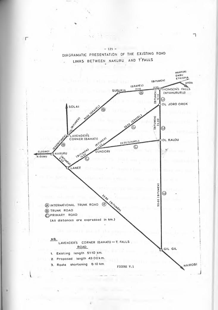
V.: “1t•I

- 125 -

DIAGRAMATIC PRESENTATION OF THE EXISTING ROAD LINKS BETWEEN NAKURU and t'falls

e m b u

kilometers is of low gravel (G.2) standard.

3. Nakuru-T. Falls via Dundori and 01 Kalou,79.2 kilometers long of which 23.0 kilometers is gravel grade (G.2).

The Bahati-T. Falls road itself is 66.5 kilometers of

which only 15.4 is to bitumen standard (Bit.II). The remaining

51.1 is earth/gravel surface with a G.2 rating on average. The

road passes through hilly and difficult terrain. The gradients

are generally steep and the horizontal alignment is characteri

zed by sharp bends and inadequate sight distances which, combined

with the narrow carriageway would tend to increase risk of

accidents and to raise VOC and journey-time for those Vho use

it. During the rainy season the road may virtually be impassable

mainly due to poor drainage. At such times traffic must use one

of the above three alternative routes. When the rains are

exceptionally heavy the earth/murram sections of the Nakuru-

Dundori-01 Joro Orok and Nakuru-Dundori-01 Kalou routes may

also be difficult to travel on and those who do not mind the

distance may go all the way via Gilgil.

The primary aim of the proposed improvement then is to

reduce vehicle operating costs and journey time for those who

use or would use the Bahati-T. Falls road. In doing so the

risk of accidents on the road will, hopefully, also be reduced

to a minimum. The upgrading will consist of reconstructing

the road to Bit. I standard with a carriageway of 7.0 meters and

a design speed of 80 kmp. The works will involve recentering,

reshaping and paving. A completely new alignment will be

- 127 -

followed where necessary in order to improve sight distances

and to reduce gradients. The length of the existing route will

be reduced from the present 51.1 kilometers to 43.0 kilometers.

5.11 AREA OF INFLUENCE

The greater part of the road lies in Nakuru district.

The impact of the proposed improvement will probably be

greater in the Bahati, Subukia and Dundori areas and the south-

western parts of Laikipia district. All these are very impor

tant agricultural areas producing wheat, maize, barley, coffee,

tea, horticultural products, pyrethrum, milk, woot, etc. The

fruit and vegetable canning factory at Kabazi also stands to

benefit if the road is paved. The improvement would be a

boon to the tourist industry as it would provide a much needed

link between Nakuru and T. Falls. From the traffic Origin-

Destination (OD) survey done on all the four roads linking

Nakuru and T. Falls and discussions with the local tour operators

and hotel managers, there is a strong indication that virtually

all the tourist traffic that presently travels between Nakuru

and T. Falls via Gilgil would prefer the Bahati-Subukia route

if it were improved. For one thing, it would be shorter; and

moreover, the route itself with the valleys and escarpments is

a tourist attraction.

The main population centers are the two townships

(Nakuru and T. Falls). This being mainly a large scale farm

ing area the population in the outlying rural areas tends to

128 -

concentrate around the rural market centers, most of which are

situated along the four roads. Population density is lighter

in the farms. The following table indicates the approximate

sizes and densities of population in the districts in which the

area of influence for the Bahati-T.Falls road lies as well as

the projections of future population growth trends for both

the districts and the principal townships:

POPULATION PROJECTIONS AND LAND AREAS FOR THE DISTRICTS SERVED

DistrictLand Area (sq. km.) Total Population „PopulationDensity

1969 1976 1986

Nakuru 7,024 291,000 372,000 531,000 53Nyandarua 3,528 177,000 227,000 403,000 64Laikipia 9,718 66,000 73,000 82,000 8

TABLE 5.2 (a)

POPULATION PROJECTIONS FOR THE MAIN TOWNS

TOWN P O P U L A T I 0 N

1969 1976 1986

Nakuru 47,000 70,600 126,400

T. Falls 7,600 13,000 29,600

«TABLE 5.2 (b)

1295.12 SCONOMIC ACTIVITY

The most important activity in the area is farming.

Light industries engaged mainly in processing farm produce are

concentrated in Nakuru town. Nakuru and T. Falls are also

tourist centers as they lie on the western fringes of the main

"tourist zone" in the country.

(U A G R I C U L T U R E

The area of study lies in one of those parts of the

country which were formerly referred to as "scheduled areas".%

Although it is still predominantly a large-scale farming

area, considerable changes have taken place in the ownership

of land. Some of the farms have been purchased from European

settlers and broken down into small scale settlement holdings.

Other farms have been bought by co-operative societies, private

companies and individuals who still operate them as large-

scale units.

The main crops grown in the area are coffee, tea,

pyrethrum, wheat, maize, a variety of vegetables and pulses

and potatoes. Livestock is predominantly cattle but there

are also some sheep and pigs,

a) Large-Scale Farms: ,

Crop Production

The table overleaf gives in summary form some indica

tion of the crop areas, average annual crop production and

its value for the years 1972 and 1973.

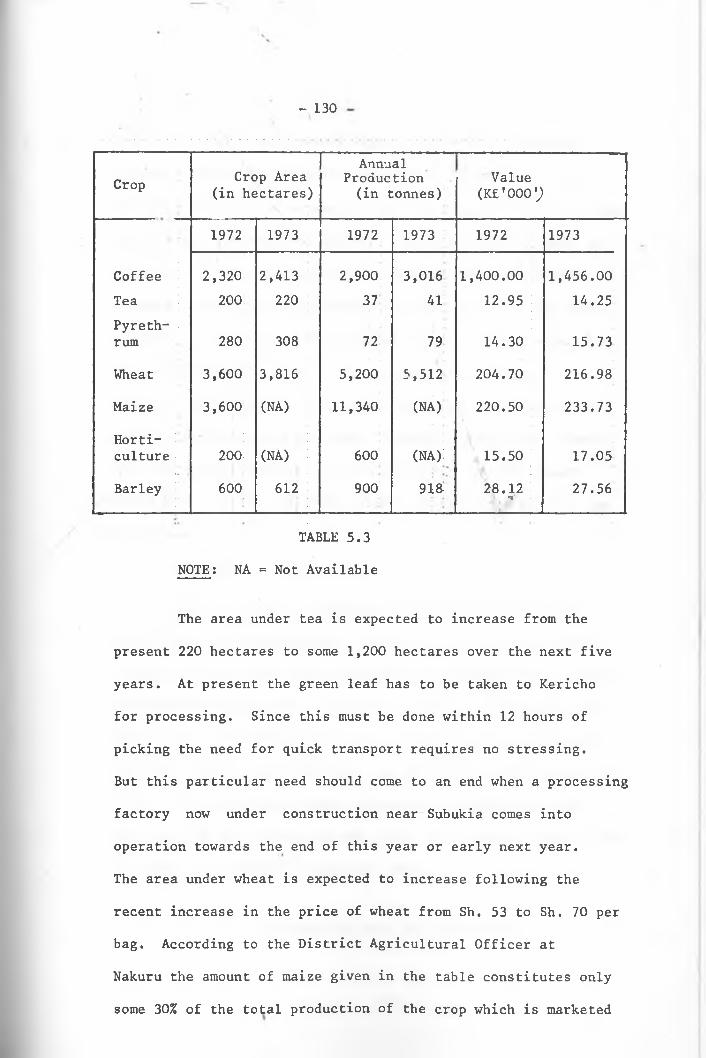
- 130

Crop Crop Area (in hectares)

Annual Production (in tonnes)

— Value (K£ '000')

1972 1973 1972 1973 1972 1973

Coffee 2,320 2,413 2,900 3,016 1,400.00 1,456.00Tea 200 220 37 41 12.95 14.25Pyreth-rum 280 308 72 79 14.30 15.73

Wheat 3,600 3,816 5,200 5,512 204.70 216.98

Maize 3,600 (NA) 11,340 (NA) 220.50 233.73

Horti- ;culture 200 (NA) 600 (NA): 15.50 17.05

Barley 600 612 900 91S 28.12V 27.56

TABLE 5.3

NOTE: NA = Not Available

The area under tea is expected to increase from the

present 220 hectares to some 1,200 hectares over the next five

years. At present the green leaf has to be taken to Kericho

for processing. Since this must be done within 12 hours of

picking the need for quick transport requires no stressing.

But this particular need should come to an end when a processing

factory now under construction near Subukia comes into

operation towards the end of this year or early next year.

The area under wheat is expected to increase following the

recent increase in the price of wheat from Sh. 53 to Sh. 70 per

bag. According to the District Agricultural Officer at

Nakuru the amount of maize given in the table constitutes only

some 30% of the total production of the crop which is marketed

- 131

through the Maize and Produce Board. The rest is consumed•« _ \ «

locally. Barley is not a very significant crop in the area.

But grassleys are, on account of the large population of cattle

in the area. It was not, however, possible to obtain data on

this crop. Horticultural crops (such as tomatoes, onions,

cabbages, beans, peas, potatoes) are grown widely in the area.

In fact, this is the chief source of supply of these items for

Nakuru and Nairobi. Some of the produce is also sent to

Mombasa. Encouraged by good export prospects the Ministry of

Agriculture intends to encourage farmers to double the output

of horticultural produce. But it is likely that the local

market which is also expanding rapidly will absorS most of the

production.

Livestock

Cattle, a large percentage of which are dairy cows

and heifers, are the principal livestock item. The population

of sheep and pigs has been decreasing at an annual rate of some

11% according to the 1972 livestock census by the Ministry of

Agriculture. According to the same census the annual slaughter

rates for cattle, pigs and sheep are 30%, 80% and 40% respec

tively. The table below shows figures on the population of

livestock and the production and value of livestock products for

the large scale farms for the year 1972:

(Please turn over for the table)

%

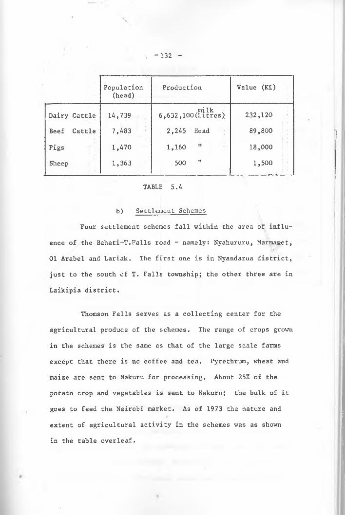
\ - 1 3 2 -

Population(head)

Production Value (K£)

Dairy Cattle 14,739mi lk . 6,632,100(Litres) 232,120

Beef Cattle 7,483 2,245 Head 89,800

Pigs 1,470 1,160 18,000

Sheep 1,363 500 " 1,500

TABLE 5.4

b) Settlement Schemes

Four settlement schemes fall within the area of influ

ence of the Bahati-T.Falls road - namely: Nyahururu, Marmanet,

01 Arabel and Lariak. The first one is in Nyandarua district,

just to the south of T. Falls township; the other three are in

Laikipia district.

Thomson Falls serves as a collecting center for the

agricultural produce of the schemes. The range of crops grown

in the schemes is the same as that of the large scale farms

except that there is no coffee and tea. Pyrethrum, wheat and

maize are sent to Nakuru for processing. About 25% of the

potato crop and vegetables is sent to Nakuru; the bulk of it

goes to feed the Nairobi market. As of 1973 the nature and

extent of agricultural activity in the schemes was as shown

in the table overleaf.

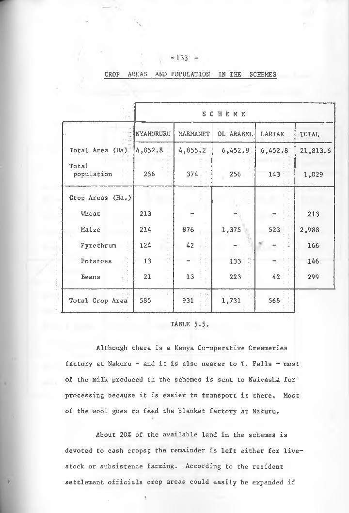
-133

CROP AREAS AND POPULATION IN THE SCHEMES

S (: h e m e•

NYAHURURU MARMANET 0L ARABEL LARIAK TOTAL

Total Area (Ha) 4,852.8 4,855.2 6,452.8 6,452.8 21,813.6

Totalpopulation 256 374 256 143 1,029

Crop Areas (Ha.)

Wheat 213 - - - 213

Maize 214 876 1,375 523 2,988

Pyrethrum 124 42 - 166

Potatoes 13 - 1 3 3 - ! 146

Beans 21 13 223 42 299

Total Crop Area 585 931 1,731 565

TABLE 5.5.

Although there is a Kenya Co-operative Creameries

factory at Nakuru - and it is also nearer to T. Falls - most

of the milk produced in the schemes is sent to Naivasha for

processing because it is easier to transport it there. Most

of the wool goes to feed the blanket factory at Nakuru.

About 20% of the available land in the schemes is

devoted to cash crops; the remainder is left either for live

stock or subsistence farming. According to the resident

settlement officials crop areas could easily be expanded if

%

_ 134

need be. The following two tables summarize the crop and live

stock production data for each of the settlement schemes for

1973.

S C H E M E TOTAL FOR ALL SCHEMES

Crop Nyahururu Marmanet)1 Arabel & Lariak Quantity Value

(K£'000')

Wheat (tonnes} 249.21 - — 249.21 6.23Maize " 254.70 1,890.00 i, 099.50 6,244.20 123.18

Pyrethrum " 30.65 3.76 - 34.40 6.88

Potatoes " 117.00 - .,197.00 1,314.00 14.60

Beans " 22.77 14.04 285.66 322.47 14.32

Livestock

Dairy Cattle(Hd)

Beef "

Sheep & Goats

Poultry (birds)

2090(900)

780

2241(1169)

3214

Milk (litres)

Wool (tonnes)

494.18

2.99

2861(1387)

933

1718(928)

3390

782.98

1389(954)

1208

380(247)

4565

60.01

6,340

2,921

4,339

11,169

1,337,164

2.99

Note;

U)

TABLE 5.6

Figures in brackets in the above table refer to livestock under one year.

(ii) Only a very small proportion of the livestock and livestock-based products is marketed and it would have been misleading to place sales values beside production figures in the table.

- 135 -

These figures (sales values) are given in the table below:

S C H E M ETOTAL

FOR ALL SCHEMES

Nyahururu Marmanet01 Arabel & Lariak Quantity

Value(Kf'OOO

Milk 4,976 (NA) (NA) 4,976 1,472

Beef Cattle - 246 25 271 813

Sheep & Goats 81 81 15 177 531

Poultry 3,214 3,290 4,568 11,072 2,180

Wool 2.99 - - 2.99 1,195

TABLE 5.7

c) Non-Settlement Co-operative Farms

These are primarily large-scale farms but in which indivi

dual members of the co-operatives are alloted plots for growing

subsistence crops. The total production from the farms and

their values for the year 1973 are shown below:

(a) CROPS:QUANTITY(Tonnes)

VALUE K£'000'

Wheat 727.40 14.47

Maize 570.87 10.74

Pyrethrum 2.39 1.51

Barley 308.34 9.37

TABLE 5.8 (a)

- 136 -\

(b) L I V E S T O C K V A L U E(K£ '000')

Cattle (head) 307 5.95

Milk (litres) 310.97 18.76

Butter-fat (Tonnes)3.92 1.59

TABLE 5.8 (b)4

(2) T O U R I S MThe proposed road improvement will help to bring closer

the national parks and other tourist attractions in the Rift

Valley and those to the east of it especially those around

Mt. Kenya in Central and Eastern Provinces, thus completing a

"tourist road loop" connecting Nairobi, Nakuru, T. Falls,

Nyeri and Meru. The main tourist attractions at Nakuru are

the Lake Nakuru National Park with its flamingo concentration,

the huge Menengai Crater and the prehistoric sites at Gilgil

(on the way to Nakuru) and Hyrax Hill. The high falls, some

game in the Marmanet Forest and a generally mild weather attract

tourists en route to and from the Mt. Kenya and Nakuru areas to

T.Falls. The Midland and Stag's Head hotels at Nakuru offer reason

ably high standard accommodation. The T.Falls Lodge is the only

"tourist class" hotel at T. Falls. In the "peak season" these

hotels enjoy very high rates of bed occupancy. The pattern of

seasonal utilization of the accommodation facilities is as

indicated in the table that follows.

137 -

SEASONAL BED OCCUPANCY RATES AT NAKURU AND T. FALLS

Occupancy Rates

Bed Capacity Peak Off-Season

Midland 80 1300 1100

Stag's Head 89 1500-2000 600-800

T.Falls .Lodge 62 1200-1900 -

TABLE 5.9

Discussions with the managements of these hotels revealed

that occupancy rates might even be higher if the B5 road were

improved throughout all its length as this would provide an

all-year-round circular flow of tourists. As of now, the Nyeri-

T.Falls section of the road is only of gravel standard and may

be impassable in the rainy season. A rough indication of what

impact the planned road improvement might have on tourism in

the area is the fairly high percentage increase (of more than

50%) in the number of tourists who have been visiting the

T. Falls Lodge since the Nakuru-Gilgil-T. Falls was paved.

But in the light of the fact that the hotels are booked

almost to capacity during the peak season an increase in the

flow of tourists would impose some strain on the hotel facilities

during this season so that further investments in accommodation

would be necessary. Despite the relatively lower occupancy rates

in the "off-season" it would not be proper to consider this

seasonal under-utilization an indication of over-investment in

- 138

hotel accommodation in the two townships. This could be the

case only if in the peak seasons the hotels usually had excess

capacity. Further evidence that there is room for more invest

ment in tourist accommodation facilities in the area is the

proposed Baharin Lodge (100 beds) to be built by the Kenya

Tourist Development Corporation in the Lake Nakuru National

Park.

But only improving the Bahati-T. Falls segment of the

B5 road will probably not in itself generate substantial

increase in the flow of tourists to the area the new road will

be serving. Such an increase would come about if -the entire

B5 road were upgraded. Improving the Bahati-T. Falls road

will certainly have some effect on tourism in the area but such

an effect is likely to be only a marginal one.

(3) I N D U S T R Y

Nakuru town has a number of light industries the impor

tant ones of which include flour, timber and steel mills, soap,

paint, fertilizer and textile (blanket) factories, a battery

manufacturing plant and milk and pyrethrum processing factories.

Generally it is expected that the proposed road upgrading will

have some bearing upon these industries in varying ways and

to differing degrees. The industries engaged in processing

farm produce such as milk and pyrethrum will probably be the

greatest beneficiaries. Earlier it was stated that most of

the milk produced in the area around T. Falls (which extends

to the eastern escarpment of the Subukia Valley) is collected

139 -

into a depot and T. Falls and then shipped to Naivasha - some

97.1 kilometers away - for processing. The road improvement

will most likely divert the milk output from this area to the

Nakuru plant. But then the Naivasha milk factory has a much

larger capacity than that at Nakuru so that the milk produced

in the area between T. Falls and Subukia would still have to

be sent to Naivasha. There might be delays in processing it

resulting into spoilage and losses to producers. Furthermore,

there is no clear indication from the field information that

transporting milk on the existing road has been much of a

problem; except perhaps when there are unusually v.£ry heavy

rains. Pyrethrum, which is less easily perishable than milk,

has always reached the processing plant at Nakuru in a whole

some state; and the tea-factory now being constructed near

Subukia.will greatly reduce the significance of the new road

to tea growers in the area. Those who stand to benefit most

from the improved road are the vegetable producers - or more

accurately, those who transport the produce from farms to

Nakuru. But as is indicated below there is little to suggest

that the present state of the road has been a bottleneck to

increased production of vegetables or that it has occasioned

farmers prohibitive losses.

The only industrial activity of any importance outside

Nakuru town is the fruit and vegetable canning factory at

Kabazi, situated some 25 kilometers from Nakuru along the

%

140 -

present road. The factory draws its raw materials from as far

afield as Kinangop, Naivasha, Limuru, Meru and Mombasa. A small

fraction of the raw materials supply comes from the surrounding

area. The present factory can handle as much as 200 tons of

tomatoes and other vegetable material per day during the peak

operating period. The annual production capacity of the plant

is some 250,000 cartons of canned products which are marketed

by Brooke Bond Leibig (Kenya) Limited.

The existing road is the only route by which the raw

materials (and other inputs) can be brought to the factory and

the finished products transported from it. According to the

factory manager occasionally the road may be impassable,

particularly for heavy vehicles. This may cause delays in the

delivery of raw materials which in turn results in losses in

working time and delays in the shipment of finished items to

the market. If the raw materials are spoilt en route to the

factory on account of the vehicles being stuck in the mud or

due to some other mishap, the suppliers or the factory owners

- depending on who of the two is responsible for the goods

while in transit - incur losses. The benefit to the raw

material suppliers and factory owners of improving the road

would then be the avoidance of the losses that would otherwise

result from lost working time, delayed delivery of finished

goods, or damaged materials.

But the probability of these losses occuring during

any one year does not seem to be significant. The number of

days during the rainy season the road would be impassable may

- 141 ~

not be so large: compared to the number of days the factory

is in operation they are only a tiny fraction. Moreover, the

fact that extensions had been made to the factory even before

plans to pave the road were initiated is ample evidence that

the present state of the road is not a constraint on the

operations of the factory. Undoubtedly, the proposed road

improvement would benefit the factory and its suppliers of

inputs. But the gain would probably not be so large as to

deserve the time and effort required to estimate it.

In conclusion, there seems to be little reason to

suppose that the new road by itself will have any substantial' i , «r

impact on the farming activities in the area of its influence.

The area is fairly well developed agriculturally, the present

road has so far been reasonably adequate: the roads have not

been a serious bottleneck to expansion in agricultural output.

In fact, to effect further output increases it is likely that

other investments, apart from those in transport, would be

necessary. Similarly, the effect of the road improvement upon

the other two economic activities, namely - tourism and

industry - will probably not be much. Consequently, no effort

has been made in this paper to estimate what would be the net

effects on the outputs of these activities of paving the

Bahati-T. Falls road. Moreover, to be able to do this, it

would have been necessary to secure more detailed information

about the functional relationships between the inputs and out

puts for the different production activities. In the light

of time and financial constraints no more than the total%

142 -

production data presented in the tables in the foregoing pages

could be collected.

5.2 D A T A G A T H E R I N G

The data used in the evaluation of the project in

this case study was collected with the aid of the staff of the

Planning Section of the Roads Department of the Ministry of

Works and under the direction of the Superintending Engineer

in the section. Two broad sets of statistics were collected:

one on traffic and the other on economic activity in the area‘t*

of study. A summary of the latter has already been §iven above.

Briefly, the method of collecting information on the different

main land uses - agriculture, industry and tourism - consisted

principally of interviews with a selected sample of farmers in

both the large scale and settlement farms, a fruit and vegetable

canning factory manager at Kabazi, hotel managers at Nakuru

and T. Falls, agricultural, settlement and co-operative officials

at Nakuru and T. Falls. Additional information was obtained

from the Provincial Planning Officer, the Provincial Director

of Agriculture, the District Agricultural Officer at Nakuru;

the Central Bureau of Statistics (Ministry of Finance and

Economic Planning), Ministry of Tourism, the Coffee and Tea

Boards at Nairobi.

The major part of the research effort, however, was

devoted to the collection of traffic information since this

forms the principal input for the economic evaluation of the

- 143

proposed project. The following paragraphs present a description

of the methodology that was employed in the gathering and pro

cessing of the traffic data.

5.21 TRAFFIC DATA

Traffic counts on Kenya roads started in 1952 on an

"ad hoc" basis. But since 1965 there has been a regular

program of repetitive counts undertaken by the Planning Section.

There are four types of traffic counts which have been

undertaken over the years:

a) The 60-Point Census:

Between 1965 and 1969 manual traffic counts were done four times a year at 60 randomly selected points covering all the main roads in the country. Since 1970, however, only one count is taken at each of these points every year in June/July. Each count lasts 5 days (Monday-Friday); for 12 hours for four days and round the clock on any one of the five days.

b) The 50-Point Count:

Automatic counts at 50 randomly selected points have been undertaken since 1966.Counting is continuous (starting at 7 a.m. each day) throughout the year. For ease of supervision and maintenance of equipment the points are located in the vicinity of MOW camps and police posts.

c) Other Manual Counts:

These have been done since 1952 as occasion demands. They are taken at selected points and run for 12 hours per day for 5 days and one night.The counts are done to provide supplementary information.

d) Special Counts;

These are more detailed and aim to provide a wider range of data than can be obtained through the other counts. Special counts consist of:

i) Origin-Destination (0-D) Surveysii) Vehicle Speed Studiesiii) Speed-Flow relationships

investigations.iv) Junction (and ferry) counts:

Unlike the other counts, special counts are undertaken for a road only when the road is earmarked for reconstruction and more detailed plans and economic analysis are required.

For the four roads in this study, manual, automatic

and special counts were done to provide a basis for estimating

the level of utilization of the Bahati-T. Falls road at present

and in future after it is bitumenized. The methodology thus

has three distinct phases:

1. gathering the raw traffic and other data,

2. determining the average level of utilization of the roads at present,

3. forecasting the level of utilization of the Bahati- T. Falls road when it is improved.

\ - 144 “

Present utilization of the road will be measured by

the volume of Normal traffic. Future utilization, on the other

hand, will consist of Normal, Generated and Diverted traffic.

In addition to the manual and automatic counts, 0-D

surveys, vehicle-speed surveys and junction counts were carried

out on all the four roads connecting Nakuru and T. Falls. The

four links will be referred to simply as the Bahati-Subukia,

Dundori-01 Joro Orok, Dundori-01 Kalou and Gilgil-01 Joro Orok

routes in the remainder of this paper. The surveys were carried

out chiefly by means of roadside interviews with motorists at

pre-selected points at Bahati, 01 Joro Orok, Subukia and T.

Falls. The survey results are shown in Figure V.2.

Two adjustments were done to the raw sample data to

derive the average daily traffic volume for the year on the

routes. The first adjustment was to convert the 12-hour sample

average values to their 24-hour normal traffic equivalents.

For this purpose conversion factors were worked out by the MOW

for each vehicle type. The factors are given in the table

overleaf.

The second adjustment was to correct the adjusted sample

values for seasonal variations in the annual flow of traffic

for which a seasonal "Correction Factor" was established.

On the basis of the automatic counter data an overal seasonal

correction factor of 1.06 was worked out and anplied to traffic

flows on all the routes. The seasonal variations in the annual

traffic flow for the past three years as recorded by the automatic

counter at T. Falls, depicted in Figure V.3, are typical of the

variations on roads in the area of study.

145 -

%

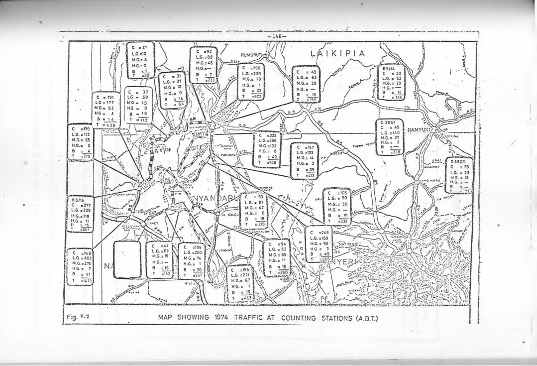
—146—

*

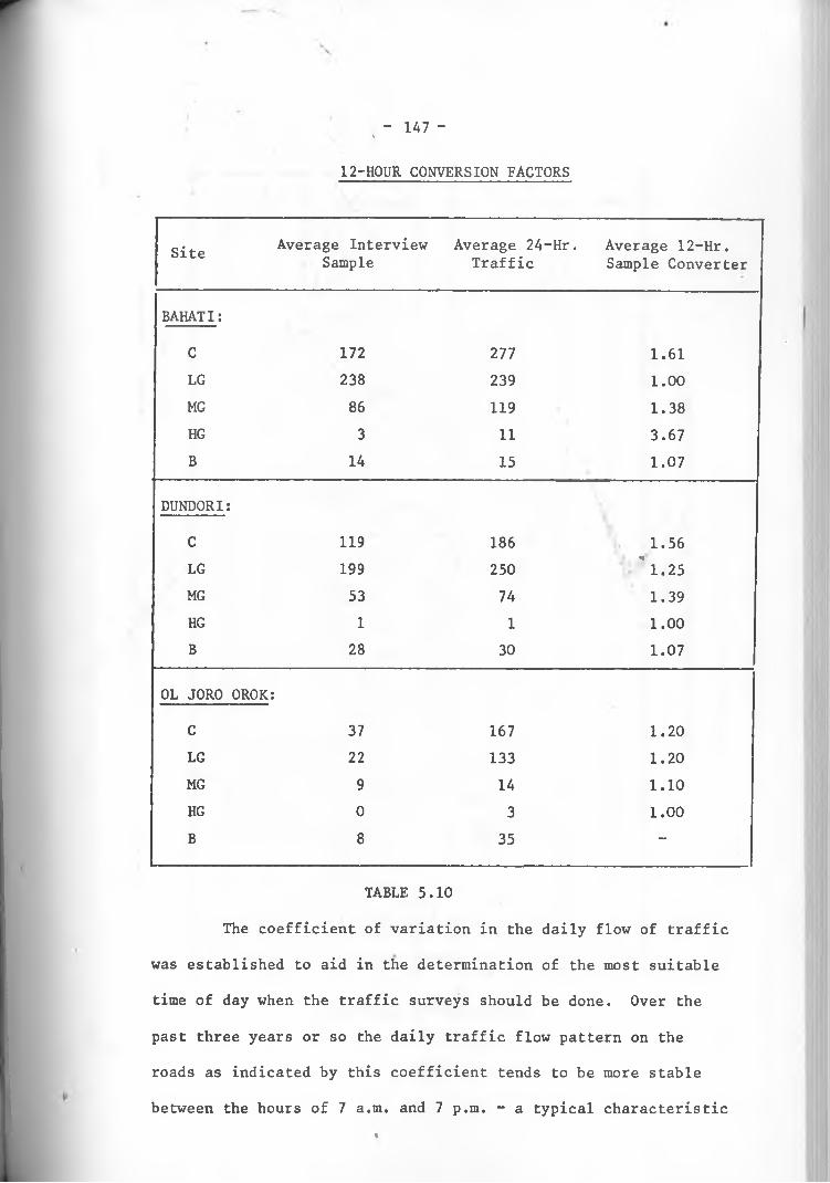
12-HOUR CONVERSION FACTORS

- 147 -

Site Average Interview Sample

Average 24-Hr. Traffic

Average 12-Hr. Sample Converter

BAHATI:

C 172 277 1.61LG 238 239 1.00MG 86 119 1.38HG 3 11 3.67B 14 15 1.07

DUNDORI

C

••

119 186 1.56LG 199 250 " 1.25MG 53 74 1.39HG 1 1 1.00B 28 30 1.07

0L J0R0

C

0R0K:

37 167 1.20LG 22 133 1.20MG 9 14 1.10HG 0 3 1.00B 8 35 -

TABLE 5.10

The coefficient of variation in the daily flow of traffic

was established to aid in the determination of the most suitable

time of day when the traffic surveys should be done. Over the

past three years or so the daily traffic flow pattern on the

roads as indicated by this coefficient tends to be more stable

between the hours of 7 a.m. and 7 p.m. - a typical characteristic%

AV

ER

AG

E

WE

EK

LY

DA

ILY

TR

AFF

IC

(A.W

.O.T

.)

- 1A8 -YEAR 1971 _ _ _ _ _

LO CATIO N ...........NYAMURURU

CLASS OF RO AD ...C 77

900

800

700

too

S00

A00

____

__ <

*

H*

i

-A- '! X

7♦♦

♦A

/1

\\\i _

A #t /

i \ii 4

* j♦

\ ! i m A / T v

// i

ii 111

//✓1

i 1 \ 1

»

/ i /

7 A/ v \

i

' a4

♦♦ ft*

*7v f \\

i V ►

V I ri \

f * \ 1

/**

•r

V

" T T 1 «

; *

r r - ♦ %

f \ /

77,rV

*1 1 #, 1

—A\ - * V

►

I i » ' /N*

V " j|A / 1 / l /

/i

♦ ♦/% > \ ^

N«1! m

• * /j \ i

riii i

i

///#

i1t\

1 * /T" ♦ / \ f \A _ a

♦ /11

¥— 7 ♦ /

r "i'X_ v N

/

T/ iii

t

i /\0

1» \

ti

»

A \ / \l " ‘ / yv /

/ w >

/ ♦ #1 *

l' ¥ \i ii i

%

iBA

ow1 TER V n s

i»ii ^

11l

\ ) L0 BAT 1CRY

■ : . i

> A1

N

i I] D I R ’Y CO ITACT P O I N T & /

- r f -

\ •

< >

\ ! o wi t t e r Y

0 2 A 6

Fig V.3

18 20 22 2A 26 28 30 32 3A 36 38 AO A2 AA A6

W EEK o f THE YEAR

50 52

ANNUAL TRAFFIC PATTERN AT SITE 45 (NYAHURURU)

I

\

of the traffic flow in the rural areas in this country. The

sample data in Table 5.11 amply illustrate this feature.

- 149 -

SUMMARY OF THE AVERAGE DAILY TRAFFIC FOR THE SURVEY WEEK

---- H----IIA . M . IIIIII

P . M •

HourIIIIII

Site Starting 7 8 9 10 11 12 ii 1 n ii

2 3 4 5 6

Bahati 8 42 57 52 58II

42 !! 55 ii

40 45 50 37 46

Dundori 8 28 42 42 41 44 " 40 33 35 36 30 37IInII

P . M . Av Mnii

Hour IIII

Starting 7 8 9 10 11 _ II * '12 n 1 n; h2 3 4 5 6

Bahati 39 33 17 14 7n

4 || 2 II_ II „3 || 3II---- H-----

4 : 5 1 - 2

Dundori 41 31 17 6 10 3 2 0 0 1

TABLE 5. 11

Indeed the counts at Bahati and Dundori sites revealed

that 85% of the traffic flow was in the period 7 a.m. to 7 p.m.

5.22 TRAFFIC AND TRAVEL SURVEYS

The surveys done on the four roads in this study were

designed to yield a wide range of information on the trips made

on the roads: their origins, destinations and purposes, as well

as information on the land uses that generate the trips. The

selection and control of the survey samples were important

phases of the survey exercise on account of the fact that%

information from the analyses of the survey data was to form

the basis of estimating total traffic and other values.

Fortunately, the continuous automatic and manual counts provided

fairly reliable but unclassified estimates of the normal ADT

(24-Hour) flows on the routes against which the results of the

sample surveys could be compared to establish their reliability

and relative accuracy.

Areal sub-divisions were made to facilitate the identi

fication and correlation of information on trips made with

economic activities. Side roads or tracks connecting the

principal junctions, mountain ranges and river courses formed

the boundaries for the subdivisions or traffic zones. The

zonal map is in Figure V.4. The main traffic generators such

as the small shopping centers of Bahati, Dundori, 01 Kalou and

01 Joro Orok were identified and treated as the centroids of

the various relevant zones.

Adequate numbers of interviewers were deployed at the

interview sites and over 90% of all the motorists passing at

the sites during the survey week were interviewed. Traffic

police from the nearby police posts helped during all hours

of interviewing to supervise and control traffic. For each

trip the vehicle type and occupancy, origin, destination and

purpose of the trip were recorded. In addition the goods

carried were recorded for commercial vehicles.

Manual counts and other traffic surveys were done at

the centroids for five days - Monday to Friday between 7 a.m.

T 150 -

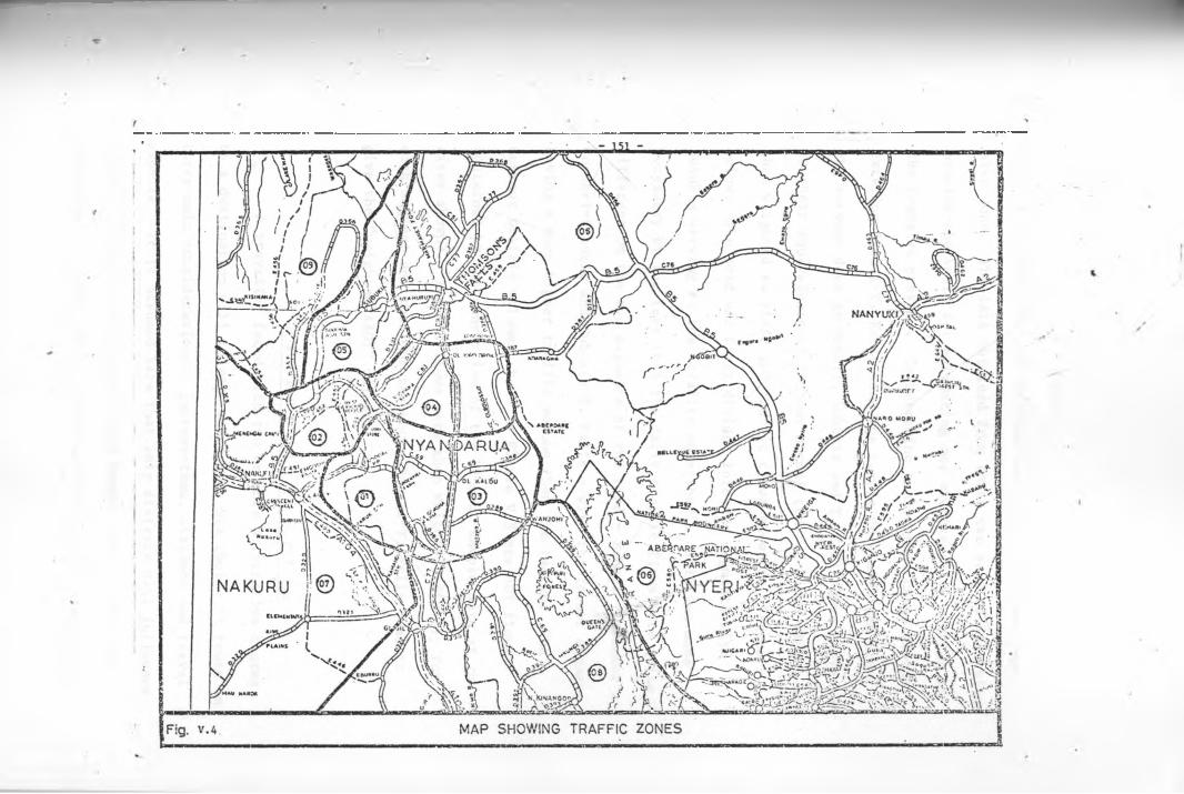
- 152 -

and 7 p.m. each day. In addition two night interviews were

also done. The data obtained from these two sets of interviews

provide the basis for estimating the average daily traffic on

the roads at present. To determine the present usage of the

existing Bahati-T. Falls road the sample data obtained from

the surveys done at Bahati, Subukia and T. Falls were converted

to their equivalents of 24-hour normal traffic flows (ADTs) and

then weighted to yield the traffic flows shown in Figure V.5

below. The road was first divided into two segments with

Subukia serving as the "traffic watershed". This was made

necessary by the fact that the daily traffic flows were quite

different on the two segments of the road - Bahati (Lavender's

Corner)-Subukia and Subukia-T. Falls - with the former segment

having a much higher traffic volume than the latter. The

current traffic volumes shown in Figure V.5 are ADT flows

(obtained by the conversion of the 12-hour sample data at the

sites shown). The ADT flows were then weighted, firstly for

each segment and then for the whole Bahati-T. Falls road to

give the "weighted AADT" values.

D i v e r t e d T r a f f i c A traveller faced with two or more alternative routes

to a destination will in many cases base his choice of route on

three main considerations: journey-time, distance and travel

expense. It is assumed here that only distance will influence

travellers' choice of route between Nakuru and T. Falls when

the Bahati-T. Falls road is paved so that all "non-essential-%

-

- 153 -

CURRENT (1974) TRAFFIC VOLUMES (A.A.D.T.) ON EXISTING LAVENDERS CORNER - T FALLS ROAD

TH O M SO NSFA LLS

LAVENDER'S C O R N ER - SUBUKIA SEG M ENT .W E IG H TE D A A .D .T .

Y E A R c. L .G . M .C . H .G . B. T.

9 4 113 4 9 2 12 2 7 0

FIGURE V.5

SU3UKIA - T FALLS SEG M ENT W E IG H T E D A.A.D.T.

Y E A R C . L .G . M .G . H .G . B . T.

1 9 7 4 S3 SB 2 9 - I t 161

LAVENDERS C O R N E R -T. F^L LS (TH E E N TIR E R OAD) W E IG H T E D A.AD.T.

Y E A R

—

C.

—

L .G . M .G . H.G. 8 T.

1 9 7 4 81 9 2 4-1 1 12 2 2 7

J

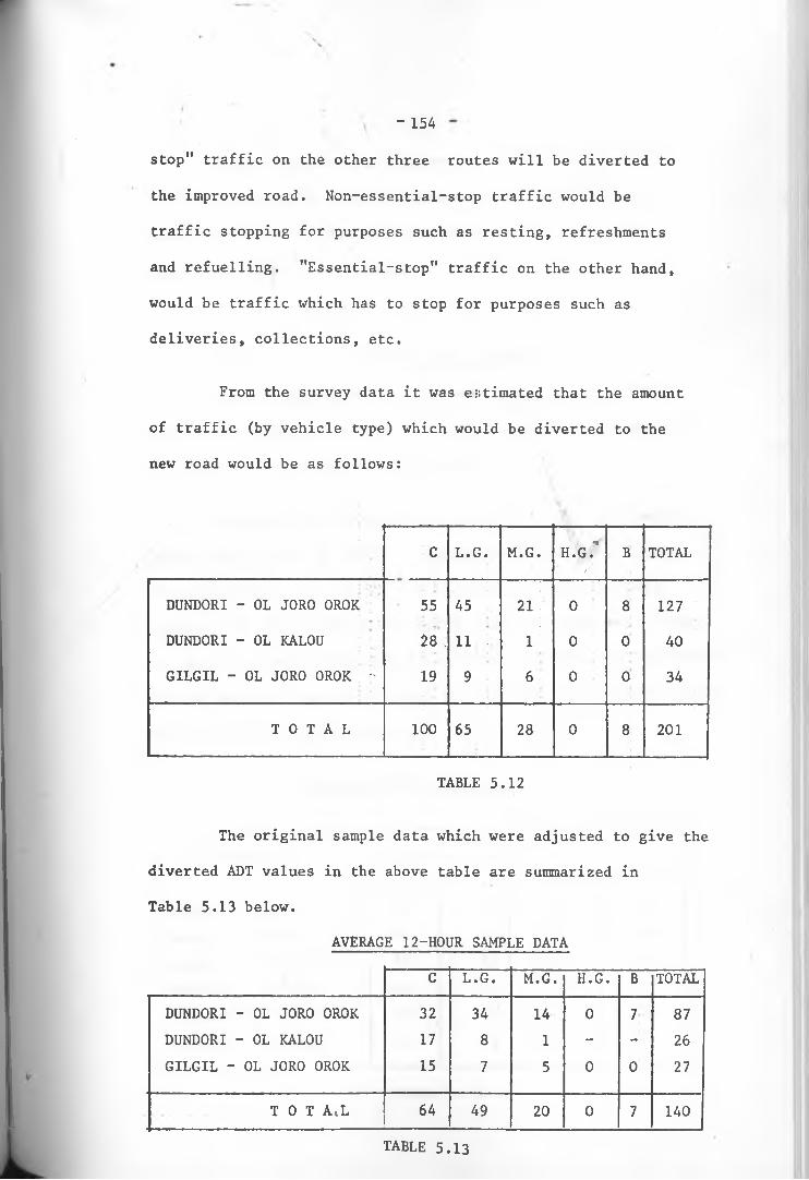
- 154

stop" traffic on the other three routes will be diverted to

the improved road. Non-essential-stop traffic would be

traffic stopping for purposes such as resting, refreshments

and refuelling. "Essential-stop" traffic on the other hand,

would be traffic which has to stop for purposes such as

deliveries, collections, etc.

From the survey data it was estimated that the amount

of traffic (by vehicle type) which would be diverted to the

new road would be as follows:

C L.G. M.G. H.G.’*’• * .

B TOTAL

DUNDORI - OL JORO OROK 55 45 21 0 8 127

DUNDORI - OL KALOU 28 ... 11 : 1 0 0 40

GILGIL - OL JORO OROK ;; 19 9 6 0 0 34

T O T A L 100 65 28 0 8 201

TABLE 5.12

The original sample data which were adjusted to give the

diverted ADT values in the above table are summarized in

Table 5.13 below.

AVERAGE 12-HOUR SAMPLE DATA

C L.G. M.G. H.G. B TOTAL

DUNDORI - OL JORO OROK 32 34 14 0 7 87DUNDORI - OL KALOU 17 8 1 - - 26GILGIL - OL JORO OROK 15 7 5 0 0 27

T O T A*L 64 49 20 0 7 140

TABLE 5.13

- 155 -

These 12-hour sample values were firstly converted to

24-hour normal traffic (ADT) flows and then corrected for

seasonal variations from their respective norms (automatic

counter daily traffic averages).

5.23 JOURNEY-TIME SURVEYS

To a large extent the cost of a journey depends on

the average speed at which it is made. Speed in turn determines

the length of time the journey takes.

Journey-time surveys were done on all the four routes

between Nakuru and T. Falls. Journey-time cards were issued

to motorists at the interview sites and at T. Falls. Cards

issued at T. Falls were collected at the sites and those issued

at the sites were collected at T. Falls. Following is a summary

of the average speeds determined for the different vehicle types

On the various route segments:

AVERAGE SPEEDS IN KM./HR.

ROUTE SEGMENTVEHICLE CATEGORY

C LG MG HG B

NAKURU - BAHATI 80 70 65 60 65NAKURU - GILGIL 90 70 65 60 65LANET - NDUNDURI 80 65 60 55 60BAHATI - T.FALLS 60 55 50 40 45DUNDORI-OL JORO OROK 70 60 55 50 55DUNDORI - OL KALOU 65 60 55 50 55

%TABLE 5. 14

- 156 -

5.24 T R A F F I C F O R E C A S T S

In Hans Adler's15 words,

"estimating future traffic is still an imprecise - but essential - art".

Road and most other transport investments last long so that

the decision to undertake them must necessarily be based on

long term forecasts. A necessary consequence of this is that

a greater degree of uncertainty is brought to bear upon the

results of the economic evaluation of projects in this area.

Traffic forecasting falls into three main stages -v *

namely:

1) estimating the volume and location of future agricultural, industrial, mining and other economic output and consumption.

2) translating output and population information into traffic data - by volume, origin and destination.

3) determining what proportions of the total expected traffic volume will be carried by the different modes of transport available.

Since future traffic depends on developments in economic

activity its estimate can be no more accurate than the fore

casts of economic growth and development.

The next step would be to establish the relationship

between these traffic generating activities and growth in

traffic volume. To this end sophisticated mathematical models

15H. Adler, Op. Cit, p. 16

157 -

have been formulated. But, as Adler points out the traffic

generators "are frequently complex and construction of the

models difficult and time-consuming." Secondly, there is the

statistical problem of insufficient and/or unreliable data.

The MOW Planning Section use the more conventional

technique of "Trend Analysis" to forecast future traffic .

Traffic forecasts are based on past traffic growth trends as

shown by traffic counts and 0-D and other surveys. The growth

rates derived from analysis of past traffic behaviour patterns

are, with modifications, used to project future trends.

The growth rates that were applied to estimate

future traffic on the Bahati-T. Falls road were derived from

the post-bitumenization data collected on three roads over a

period of some four years. In view of the brevity of this

period and in the light of the economic events that have

taken place both at home and abroad in recent times, the rates

may not be very reliable indicators of future traffic develop

ments. But for purposes of this case study they will do.

The roads used in deriving the rates were:

1. Gilgil - T. Falls (C 77)

2. Athi River - Namanga (A 104)

3. Ahero - 'Isabenia (B 4)

The last two roads are not indicated in the map in

Figure V.2. The second one is a section of the so-called

Great North Road connecting Arusha and Nairobi - Namanga

being a border post. Similarly, the third road is just a

if

segment of the road linking the two Lake Victoria ports of

Kisumu and Mwanza. Isabenia is another border post on the

Kenya-Tanzania boundary. Additional information was also

obtained from vehicle registration records and the 1970-73

60-Point Census. The growth rates which were derived are

tabulated below:

158 -

c L.G. M. G. H. G. B

1st 5 years % 12 12 10 13 10

2nd " " Growth 10 10 9 11 9For the rest of Project life

Rates9 9 8

' y 9 8

TABLE 5.15

Basically these rates were applicable to all the three

traffic categories: Normal, Generated and Diverted traffic.

However, to take cognizance of the fact that generated traffic

tends to grow rapidly in the first few years after the paving

of a road and then to revert to the normal growth pattern, it

was assumed that generated traffic would be some 10% of the

normal traffic in the first year, 15% in the second year and

20% in the third year after butumenization. After this

generated traffic would grow at the normal growth rates shown

above. Clearly if this assumption is valid, it will not be

until the second 5-year period after bitumenization that

generated traffic will fully revert to the normal traffic growth

pattern.

\

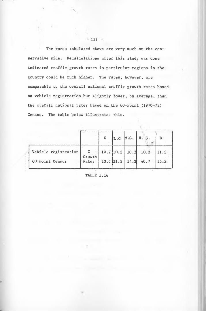
The rates tabulated above are very much on the con

servative side. Recalculations after this study was done

indicated traffic growth rates in particular regions in the

country could be much higher. The rates, however, are

comparable to the overall national traffic growth rates based

on vehicle registration but slightly lower, on average, than

the overall national rates based on the 60-Point (1970-73)

Census. The table below illustrates this.

- 159 -

5 . .

C L.G M.G. H. Q . B

Vehicle registration %Growth

10.2 10.2 10.3 10.3 11.5 ;

60-Point Census Rates 13.6 21.3 14.3 40.7 15.2

TABLE 5.16

5.3 ECONOMIC ANALYSIS

The economic valuation of a project consists essentially

of comparing its costs with the benefits in order to determine

its net worth to society. The costs for a road project consist

of the initial capital outlays and the recurrent expenditures

incurred to keep it in proper running condition. The more

significant benefits are in the nature of savings: savings in

road users' costs, journey time, maintenance costs and reductions, (

in accident risks. The actual computation of the costs and

benefits associated with a road project is the main concern ofy*

this chapter. The computational procedure adoptednhere is

similar to that followed by the MOW. There are, however, some

differences in the treatment or definitions of some specific

items.

5.31 COMPUTING PROJECT COSTS

The physical (engineering) basis of determining con

struction and maintenance costs is the Bills of Quantities

document prepared by the MOW or, as is generally the case, by

a consultant for the MOW. The document sets out the details

of the works to be carried out and the construction or

maintenance cost rates applicable to each of the works items.

The following is a summary of Bills of Quantities showing

the estimates of the cost items for the proposed Bahati-T. Falls

road.

Item Description Amount (KSHS.)

i)ii)

iii)

iv)v)

vi)

vii)viii)

ix)x)xi)

xii)

xiii)

xiv)

Preliminary and general expenses Site clearing

841.320.00968.600.00

Earth Works for formation of road pavement (7.0 m.)

Gabion wallsCulverts and drainage worksMaintenance of existing road and

diversionsWater-bound road baseSub-base and shouldersBituminous surfacingConcrete framework and reinforcementsRoad furniture

Schedule of Dayworks @ 2^%

S U B - T O T A L

Contingencies @ 7^% of sub-total

TENDER SUM (based on MOW 1970 rates)

Reduce to 92% for lowest tender

16.634.041.00771.000. 00

2,858,132.20

750.000. 00 3,658,617.50 4,724,432.00 2,441,794.70500.000. 00 899,480.00

35.047.418.00 876,185.50

35,923,603.50

2,694,270.30

38.617.873.80

35.528.443.80

xv) Escalate @8% p.a. for 41; years to assumed m.p.c., Dec. 1975 51,207,146.00

or £2,560,357; an average of £59,500 per km.

NOTES: 1

1. The MOW use this engineering cost estimate as a norm- for assessing tender bids for a project. When offers have been received from contractors the average of the lowest three tenders is used as a rough standard against which the engineering estimate itself is also checked. Normally, the difference between this average and the consultant's (or the Ministry's) estimate is a minor one. Also the lowest tender bid is usually some 92% of this average

162 -

while the highest rarely exceeds the average by more than 8%. Other things being equal, the successful bidder would be the one who bids lowest. This "ceteris paribus" assumption seems a reasonable one to make since at the time the engineering cost estimates are made "other things" about potential bidders, including who these might be, are not known - especially when the estimates are made so long in advance (3 years in the case of the road project in question here).

2. Contingencies, allowed at 7|%, provide for unforeseen increases in works quantities. Some of the factors which necessitate this provision include:

(i) exceptionally heavy rains

(ii) presence of rock or some other hard material,

(iii) changes in road alignment

(iv) changes in type of pavement material.

The proportion of the contingency provision to total cost varies according to the physical conditions which in turn are the principal determinants of the engineering design and - hence - the cost estimates.

3. Escalation "is a sum of money(expected to be spent) as an additional works cost to account for the mid-pointof any contract (m.p.c.) being at date later than the fixed base used in preparing engineering estimates."16 Escalation caters for trends in unit (cost) rates and changes in the purchasing power of money. The works cost rates are contained in a document entitled Analysis of Contract Rates based on rates furnished by contractors.The rates are subjected to close scrutiny by the MOW staff or their consultants before they are accepted as reasonable.

’ %

16MOW "Road Loan Application: Highways V", September 1972, pp.33-34.

- 163 -

The amount of escalation depends partly on the point in time when the works are expected to be executed. The actual amount of escalation can be read off the MOW "Escalation Graph" which compares actual road construction costs with contract rates tendered. Escalation rates vary from as low levels as 1.5% to 12% per annum depending on the size of the contract which generally ranges from £100,000 to substantially much larger amounts (of £3 million or more).

4. Works supervision is usually done by consultants (e.g. Alexander Gibb &Partners, E.A. Consultants, John Burrow & Partners, etc.). The Ministry prefers that a consultant supervise the project he designs,which is in accordance with the Standard Design and Supervision Agreement to which the.MOW and the Kenya Association of Consulting Engineers (1970) are party.

Supervision costs are calculated as a percentage of the total works costs and vary inversely with the size of a contract. On high cost contracts it may be as low as 6%; on low cost contracts it may be anything from 12% to 25%.

5. Contracts are awarded through a competitive tender system in accordance with either the "Guidelines Relating to Procurement Under IBRD and ADB Credits" or alternatively in accordance with the more universally accepted "Conditions of Contract (International) for Works of Civil Engineering Construction" prepared by "Internationale des Inginieurs - Conseils and Federation Internationale des Entrepreneurs European de Batimetet de Travaux Publics" with the approval of Asian and Western Pacific Contractors Association.17

While the size of a contract is an important consideration in awarding a job to a contractor, it is by no means the case that the lowest bidder always wins. Other considerations which

17 MOW, "Highways V",September 1972, p. 37.

- 164 -» V

may even be more important in awarding a contract include the contractor's experience, the capacity in terms of the amount and quality of his equipment, technical personnel, financial resources, etc.

Once a contractor has been awarded a contract he may not

alter his contract rates. The rates will have been determined

on the basis of market prices and, given the competitiveness of

the tender system and the international market in which most

of the road construction inputs are bought it can be assumed

that the market prices for the inputs are good enough approxi-

mations of the inputs' opportunity cost values. It thent V

remains to adjust the market prices to obtain the social

opportunity cost values of the inputs. But rather than attempt

to compute the SOC of each input item separately the MOW have

found it more practicable to firstly estimate the total

financial cost of a project and then to adjust this cost to get

its economic equivalent measure.

Three adjustments are done to convert financial to

economic costs. Taken together the three adjustments constitute

the shadow-pricing of the inputs. Three categories of inputs

items are shadow-priced:

(a) FOREIGN EXCHANGE

A very large proportion of construction (and maintenance)

costs are in FE. The foreign exchange component (FEC) in these

costs can easily be derived from the MOW's Analysis of Contract

Rates (1971) document as well as from information provided by

%

- 165 -

private contractors. The basic assumption in the derivation

of the FEC is that the official exchange rate understates the

true value of FE (or conversely, overstates that of the

domestic currency) to the economy. The following table

summarizes the estimated foreign and domestic currency or

"internal exchange" components in the total construction

costs for the proposed Bahati-T. Falls road.

v • As a % ofTotal Cost

I T E M Item as a % FEC IECof Total % % FEC IEC

Cost

1. Capital equipment 18 95 5 17.10 0.90

2. Materials:(a) bitumen 6 85 15 5.10 0.90(b) cement 9 85 15 7.65 1.35(c) stone 9 40 60 3.60 5.40

3. Fuel and Oil 6 85 15 5.10 0.90

4. (a) Design and con-struction overheads 27 60 40 16.20 10.80

(b) Engineering super- 1 •vision 10 50 50 5.00 5.00

5. Unskilled labour 10 10 90 1.00 9.00

6. Miscellaneous 5 85 15 4.25 0.75

65 35

TABLE 5.17

NOTES:

(i) Capital equipment consists of a host of itemssuch as bulldozers, scrappers, rollers, tippers,

%

- 166 -

shovels, etc. Detailed break-downs of costs on the basis of these specific items have been worked out by the MOW and the FEC in the cost of each could easily be determined if need be.

Design and construction overhead costs consist of the cost of MOW design work or that of consultants.

The FEC in the engineering supervision item is decreasing steadily with the advance of Africanization.

The small FEC in the cost of unskilled labour reflects the estimated proportion of the wage bill which unskilled workers spend on imported goods.

Through similar procedure the FEC in maintenance costs

for the proposed road was estimated to be about 30% of total

financial maintenance cost bill. The shadow-pricing of FE is

effected by adding an extra 15% to the 65% and 30% FECs in the

construction and maintenance costs respectively. The "FE con

version factor" is, therefore, 1.15.

(b) TRANSFER PAYMENTS

The second adjustment to the financial costs relates

to such transfers as indirect taxes and subsidies of various

types on certain cost items. The adjustment is to subtract

the sum of indirect taxes from, and add subsidies to, the

financial costs. Capital goods including equipment and certain

intermediate goods are imported tax-free into Kenya. Through

its investment allowances policy the Government does subsidize

capital equipment and materials imported by private firms.

Government agencies, until recently, were exempt from local

(ii)

(iii)

(iv)

excise taxes and import duties which amounted to subsidizing

them. There was however, no indication that the government

directly subsidizes such intermediate goods as bitumen. The

indirect subsidies on capital equipment through allowances/

deductions of various sorts would have been too difficult and

time consuming to determine. Consequently, the only "transfer

payment" adjustment done to the financial costs of the proposed

road project was the deduction of indirect taxes on materials.

Until recently, the MOW was using an indirect tax rate of 10%.

Since the imposition of the 10% sales tax the rate has probably

changed (risen) although in principle the sales tax,was

supposed to replace the previous consumption tax of approximately

the same magnitude.

(c) UNSKILLED LABOUR

It is generally agreed that the market wage rate in

this country, as elsewhere in the developing world, overstates

the economic value of unskilled labour. The Central Bureau

of Statistics (in the Ministry of Finance and Economic

Planning) estimates that the SOC of this category of labour

is some 50% of the market wage rate. The financial wage

costs were therefore reduced by a half to arrive at the

SOC of unskilled labour. As indicated in Table 5.18, unskilled

labour costs constitute only about 10% of total construction

costs; but they rise to a significant 30% in maintenance costs,

reflecting the relatively more labour-intensive nature of road

168 -

maintenance work.

MAINTENANCE COSTS

The calculation of maintenance costs for gravel roads -

routine maintenance and regravelling - is based on the average

daily traffic (or vehicle per day, v.p.d.). Gravel roads are

graded by the Ministry as G4, G3, G2, G1 and GO (in descending

order) according to their surface quality, width and other

characteristics. The average maintenance cost rates for

gravel roads at different volumes of traffic are given below.18y *

Routine Maintenance <

V.P. D . cost/km._________ Regravelling

Over 300 £200 £600

200-300 180 600

100-200 140 500

50-100 120 500

0-50 80 500

Regravelling and routine maintenance cost rates vary

in different parts of the country and the MOW have worked out

rates on a provincial basis. Since the factors which determine

the magnitude of the cost rates are not confined within pro

vincial boundaries, this hardly appears an appropriate basis.

The above rates are for the Rift Valley Province but they

could very well apply to most areas in Western Kenya.

The regravelling cycle depends almost entirely on the

18 MOW, "Maintenance, Resealing and Regravelling Costs • • • ."(1974)

- 169 -

volume of traffic as shown below:

V.P.D. C Y C L E

0 - 50 Every 5 years

50 - 100 If 4 ii

100 - 200 II 3 ii

Over 200 II 2 it

For tarmac roads the annual maintenance cost rates are

given as follows:

Grade

Bit. II

Bit. I

C o s t R a t e F o r :

Routine Maintenance Resealing■ V *

£140 £650

140 700

Resealing is carried out every 5 years irrespective of traffic

volume. The rates shown for resealing are for a single coat,

assuming the resealing is done by the MOW itself. If it is

contracted out to a private firm the rates may be higher by

between 20% and 25%. If the rate of deterioration in a road

is faster than was expected, "extra-ordinary maintenance",

for which the MOW always makes a provision, must be done.

The actual calculation of the total maintenance costs

per year for the present and proposed Bahati-T. Falls roads

was done as follows:

\ - 170 -

1. Existing Road;

a) Annual routine maintenance:

Period v.p.d. v.p.d. C o s t

1974-1976 227-283 51.1 x £80 = £9,198

1977-1996 300+ 51.1 x £200 =£10,220

b) Regravelling (due in 1977):

Traffic in period 1977-1996 is over 200 v.p.d.

Therefore cost = 51.1 x 600 = £30,660 p.a.

2. Proposed Road:

a) Routine maintenance costs

= 43 x £140 = £6,020 p.a.

b) Resealing - every 6th year after bitumenization:

= 43 x £700 = £30,100 p.a.

The annual totals of these costs are shown in the Cost

Analysis Sheet (Table 5.18) for the entire 20 year estimated

life of the proposed road.

NOTE:

The contractor will hand over the new road to the MOW

at the start of 1977 - about one year after completion of

construction. So any maintenance costs incurred by the

contractor before 1977 do not enter the MOW's maintenance costs.

FINANCIAL AND ECONOMIC COST ANALYSIS:TABLE 5.13 (IN £ '000')

MAINTENANCE c o s t s c n e x i s t i n g ROAD CONSTRUCTION COSTS ON PROPOSEO ROAD MAINTENANCE COSTS ON PROPOSED HOAD

PLUS: MINUS: PLUS: MINUS: PLUS: MINUS:

Y E A Rt o t a l MINUS: SHADOW UNSKILLED EQUALS: t o t a l MINUS: SHADOW UNSKILLED EQUALS: t o t a l MINUS: SHADOW UNSKILLED EQUALS*

ESTIMATED TAXESPRICC F OR COR. EXCH

WAGE BILLSHADOW

ECONOMIC ESTIMATED TAXES PRICE FOR r OR. EXCH

WAGE BILL SHADOW

ECONOMIC e s t i m a t e d TAXESPRICE FOP FOR. EXCH

WAGE BILE SHADOW ECONOMIC

COST ;io% o r a : 05V. ON 30V. OF A )

PRICE (50 V. ON 30% Of a :

COST c o s t (10% O F F ) 05 v. c s 6 5 V . OF F )

PRICE (50V. ONTO •••OF F

COST COST CTOV.OF K) C S V . ON 30v. o r k ;

PRICE C5CV, ON 10*/. OF K

COST

A B C 0 E F G H 1 J K L M N

1 9 7 4 9 . 2 0 8 . 2 8 8 . 6 9 1 . 3 8 7 . 3 1 - - - - - - - - - -

1 9 7 5 9 . 2 0 8 . 2 8 8 . 6 9 1 . 3 8 7 . 3 1 1 0 0 0 . 0 0 9 0 0 . 0 0 9 9 7 . 5 0 9 4 7 . 5 d S 4 7 . 5 0 - - - - -

1 9 7 6 9 . 2 0 8 . 2 8 8 . 6 9 1 . 3 8 7 . 3 1 1 3 0 4 . 3 6 1 1 7 3 . 9 2 1 3 0 1 . 1 0 1 2 3 5 . 8 8 1 2 3 5 . 8 8 - - - - -

1 9 7 7 3 0 . 6 6 2 7 . 5 9 2 8 . 9 7 4 . 6 0 2 4 . 3 7 2 5 6 . 0 0 2 3 0 . 4 0 2 5 5 . 3 6 2 4 2 .5 6 1 2 4 2 . 5 6 - - - - 4.79 . .1 9 7 8 1 0 . 2 2 9 . 2 0 9 . 6 6 1 . 5 3 8 . 1 3 - - - - 6.02 5 . 4 2 5 . 6 9 0 . 9 0 4.791 9 7 9 1 0 . 2 2 9 . 2 0 9 . 6 6 1 . 5 3 8 . 1 3 - - - - - 6.02 5 . 4 2 ' 5 . 6 9 0 . 9 0 4.791 9 8 0 3 0 . 6 6 27 '. 59 2 8 . 9 7 4 . 6 0 2 4 . 3 7 - - - - - 6.02 5 . 4 5 . 6 9 0 . 9 0 4.791 9 8 1 1 0 . 2 2 9 . 2 0 9 . 6 6 1 . 5 3 8 . 1 3 - 6.02 5 . 4 5 5 . 6 9 0 . 9 0 4.791 9 8 2 1 0 . 2 2 9 . 2 0 9 . 6 6 1 . 5 3 8 . 1 3 - - - - 3 0 . 1 0 2 7 . 0 9 2 8 . 4 4 4 . 5 2 2 3 . 9 2

1 9 S 3 3 0 . 6 6 2 7 . 5 9 2 8 . 9 7 4 . 6 0 2 4 . 3 7 - - - 6 . 0 2 5 . 4 2 5 . 6 9 0 . 9 0 4 . 7 9

1 1 9 8 4 1 0 . 2 2 9 . 2 0 9 . 6 6 1 . 5 3 8 . 1 3 - - - - - 6 . 0 2 5 . 4 2 5 . 6 9 0 . 9 0 4 . 7 9

1 9 8 5 1 0 . 2 2 9 . 2 0 9 . 6 6 1 . 5 3 8 . 1 3 - - - - - 6 . 0 2 5 . 4 2 5 . 6 9 0 . 9 0 4 . 7 9

1 9 8 6 3 0 . 6 6 2 7 . 5 9 2 8 . 9 7 4 . 6 0 2 4 . 3 7 - - - 6 . 0 2 5 . 4 2 5 . 6 9 0 . 9 0 4 . 7 9

1 9 3 7 1 0 . 2 2 9 . 2 0 9 . 6 6 1 . 5 3 8 . 1 3 - - - - - 6 . 0 2 5 . 4 2 5 . 6 9 0 . 9 0 4 . 7 9

1 9 8 8 1 0 . 2 2 9 . 2 0 9 . 6 6 1 . 5 3 8 . 1 3 - - - - - 3 0 . 1 0 2 7 . 0 9 2 8 . 4 4 4 . 5 2 2 3 . 9 2

1 9 8 9 3 0 . 6 6 2 7 . 5 9 2 8 . 9 7 4 . 6 0 2 4 . 3 7 - - - - - 6 . 0 2 5 . 4 2 5 . 6 9 0 . 9 0 4 . 7 9

1 9 9 0 1 0 . 2 2 9 . 2 0 9 . 6 6 1 . 5 3 8 . 1 3 - - - - - 6.02 5 . 4 2 5 . 6 9 0 . 9 0 4 . 7 9

1 9 9 1 10.22 9 . 2 0 9 . 6 6 1 . 5 3 8 . 1 3 - - - - 6.02 5 . 4 2 5 . 6 9 0 . 9 0 4 . 7 9

1 9 9 2 3 0 . 6 6 2 7 . 5 9 2 8 . 9 7 4 . 6 0 2 4 . 3 7 _ _ _ _ 6.02 5 . 4 2 5 . 6 9 0 . 9 0 4 . 7 9

1 9 9 3 10.22 9 . 2 0 9 . 6 6 1 . 5 3 8 . 1 3 - - - - 6.02 5 . 4 2 5 . 6 9 0 . 9 0 4 . 7 9

1 9 9 4 10.22 9 . 2 0 9 . 6 6 1 . 5 3 8 . 1 3 - - - - - 3 0 . 1 0 2 7 . 0 9 2 8 . 4 4 4 . 5 2 2 3 . 9 2

1 9 9 5 3 0 . 6 6 2 7 . 5 9 2 8 . 9 7 4 . 6 0 2 4 . 3 7 - - - A . . - 6.02 5 . 4 2 5 . 6 9 0 . 9 0 4 . 7 9

1 9 9 6 10.22 9 . 2 0 9 . 6 6 1 . 5 3 8 . 1 3 - - - - “ 6.02 5 . 4 2 5 . 6 9 0 . 9 0 4 . 7 9

171 -

|

jI*

(

J

- 172 -

5.32 COMPUTING PROJECT BENEFITS

For conceptual and/or statistical reasons stated in

the foregoing theoretical statement on the measurement of the

benefits of a road project it was possible to estimate the

values of only three benefit items, namely:

(a) VOC Savings

(b) Time Savings

(c) Maintenance Cost Savings

It was felt whatever development effects the proposed road

might have in the area it traverses would be marginal.

Largely because of lack of statistics on accidents on the

existing road and also because of the possibility that the

incidence of accidents on the road is as low as it could be

on any such road it is considered that the proposed road will

confer little benefit by way of reductions in risk of

accidents. If anything it may in fact raise the incidence of

accidents. External effects would have been too involved to

trace and evaluate. Spillovers such as linkage and multiplier

effects would,like the potential development effects, probably

be negligible. It is possible there might be some income

redistribution in the form of increases in the values of pro

perties situated along the proposed route but it would

virtually be impossible to determine what proportion of it is

a net increase in site values and what proportion is a mere

transfer. It has been stated above there would be little

benefit by way of favourable spillover effects from a road

project. On the other hand even the possible unfavourable

spillover effects, mainly in the form of environmental pollution

would have negligible impact in rural Kenya.

The method adopted for forecasting future traffic on

the Bahati-T. Falls road and other routes in the area of its

influence consisted simply of escalating the ADT volumes for

the year 1974 on each of the roads by the growth rates shown

in Table 5.16 above. Clearly this is not an altogether satis

factory method of forecasting traffic but then in the nature

of things, "estimating future traffic is still an imprecise ....

art" as Adler observes. A more satisfactory method of establish

ing future traffic on the four routes would have required far

more detailed information on the economic and other factors

which have a bearing upon growth in traffic volumes than the

time constraint would allow. Moreover, the forecasting techni

ques themselves would probably be more complicated than the

writer could handle with ease. Since the field investigation

for this case study was carried out the MOW have introduced

some refinements in their forecasting techniques although the

method remains essentially that of Trend Analysis.

Except, as already stated, for Generated traffic growth

in the first three years, the growth in the volume of traffic

on all the four roads was determined simply by compounding the

1974 ADTs at the growth factors in Table 5.16. The forecasts

of Normal and Generated traffic volumes for the existing

\ - 173 -

- 174 -

Bahati-T. Falls road are shown below in Table 5.20. For the

calculation of VOC and Time Savings benefits only traffic

volumes for the period 1977-1996 are relevant. The figures

for the years 1974-1976 are shown only for completeness. The

forecasts for Diverted traffic are given in Table 5.24.

(a) VOC SAVINGS .

The VOC rates used were derived from notes by the MOW

Chief Engineer (Roads) on "Vehicle Operating Costs for Gravel

(and bitumen) Roads in Kenya 1970" up-dated to 1974. Below

is a table showing average VOC rates by vehicle type on various

grades of roads:

VOC RATES/KM. FOR 1974 IN KENYA

Grade of Road

AverageSpeedsKm/Hr.

VOC RATES (IN KSHS) BY VEHICLE TYPE

C LG MG HG B

GO 40 0.79 0.82 1.76 3.16 1.90

G1 50 0.71 0.75 1.59 2.89 1.73

G2 45 0.64 0.68 1.43 2.61 1.51

G3 55 0.56 0.61 1.26 2.34 1.40

G4 65 0:49 0.52 1.10 2.07 1.24

Bit.II 80 0.45 0.47 1.00 1.93 1.13

Bit.I 100 0.39 0.42 0.90 1.78 1.02

TABLE 5.19

175 -

The 1970 rates were averaged by the MOW out of more

detailed data provided by Alexander Gibb & Partners, the E. A.

Transport Study, the World Bank and the MOW itself. The rates

in Table 5.19 were arrived at by escalating the 1970 rates by

8% - which is the estimated average rate of inflation in the

country until late last year. Factors which were considered

to be important determinants of the magnitudes of the road

users' cost rates included:

i) riding quality of roads: gravel quality, horizontal alignment,

ii) gradients

iii) rainfall, drainage v

iv) sight distances

For purposes of this paper only the rates for G2 and

Bit. I are relevant: all the existing four roads are gravel

grade two (G2) roads; the proposed road will be a grade one

(Bit. I) road. The calculations of VOC savings per vehicle

trip are given in Table 5.21 and in Table 5.22 are set out the

total VOC savings by type of vehicle for Normal and Generated

traffic.

The expected Diverted traffic volumes for each year of the

20 year life of the proposed road are given in Table 5.24. It

was earlier stated that on gravel roads VOC rates would tend

to rise as traffic volume increases. For volumes of traffic

below 1000 v.p.d. the rates would be the normal ones given in

Table 5.17. For volumes of over 1000 v.p.d. but below 17000

the rates would be 8% higher than the normal rates, and for

- 176 -

over 1700 v.p.d. the VOC rates would be 12% higher than the

normal. For simplicity in computations it was estimated the

increase in VOC rates would rise in steps rather than

continuously.

On the three gravel roads from which traffic is

expected to be diverted VOC savings were calculated for both

Diverted and Undiverted traffic (the traffic that would continue

to use the roads after some has been diverted). The benefit»

to Diverted traffic would be the difference between the VOC

rates at given traffic volumes on the present roads (or road

segments) and the rates on the new Bit. I road. The benefits

to Undiverted traffic would be the difference between the

rates that road users would have incurred on these roads if no

traffic were diverted at all and what they would incur when some

traffic is diverted to the new road. The computations of VOC

savings for Diverted and Undiverted traffic would then be as

shown below for the Dundori-01 Joro Orok route:

Let V , = v.p.d. for any vehicle type

Vp = Diverted traffic volume

V" = Undiverted traffic

Cq = VOC rate for any vehicle type for V < 100 on gravel road segments

Cb = VOC rate on existing tarmac road segments

C^ = VOC rate on the proposed Bit. I road

%

- 177 -

Then VOC savings for:

Diverted Traffic

when

VT < 1000; 33.2 + 30.20^- 15.4 - 43.OC V .

V > 1000 < 1700; 33.2C V + 30.2(1.08Co Vn) - 15.4 CLV - 43.OC V1 D U t) b D n D

VT > 1700: 33.2 + 30.2(1.12 CQ VQ) - 15.4 C ^ - 43.0 C VD

Undiverted Traffic

(a) when VT > 1000 < 1700ji*

■ without proposed road

VOC = 30.2(1.08 qjV")

with proposed road

VOC = 30.2 CQV'

Savings benefit due to some traffic diversion

» 30.2(1.08CqV' - 30.2 C0V')

= 30.2(0.08 C0V')

(b) when VT > 1700

without

VOC = 30.2(1.12 C0V")

with

VOC <= 30.2(1.08 C0V')

VOC savings *= 30.2(1.12 C0V') - 30.2 (1.08 C0V')= 30.2(0.04 C0V')

- 178 -

Note

1. For Undiverted traffic volumes of less than 1000 v.p.d. there would be no savings in road users' operating costs since the cost rates on all the existing roads would be the normal ones (CQ).

2. Similar calculations would yield the VOC savings for Diverted and Undiverted traffic on the Dundori-01 Kalou route. There would be no VOC savings benefit for Undiverted traffic on the Gilgil-01 Joro Orok route because it is tarmac throughout its whole length and it has been assumed VOC rateson tarmac roads remain unchanged irrespective of traffic volume.

The resultant VOC savings per vehicle per annum on each

of the three routes - namely: Dundori-01 Joro Orok, Dundori-

01 Kalou and Gilgil-01 Joro Orok are presented in Tables 5.25,

5.26, and 5.27 respectively. The corresponding total annual

VOC savings for each vehicle type are set out in Tables 5.28

and 5.29. Undiverted traffic on each route would simply be

the difference between total traffic volume on each route

(See Table 5.23) and the traffic volume expected to be diverted

from it (shown in Table 5.24). Undiverted traffic volumes for

Dundori-01 Joro Orok and Dundori- 01 Kalou routes after the

new road is opened are given in Table 5.30. No similar traffic

figures are given for the Nakuru-Gilgil-01 Joro Orok route.

Such traffic would not enjoy any VOC savings benefit. Nor was there

any reason to show the total traffic volume on that route since

it would not be required for the determination of Undiverted

traffic.

FORECAST TRAFFIC ON PROPOSED ROADTABLE 5.20 _____________________________________ AADT

YE N O R M A L G E N E R A T E D T O T A L

AR CARS

LIGHTGOODS

KSXUMGOODS

HEAVYGOODS

BUSES T O T A L CARSLIGHT

GOODSMEDIUMGOODS

HEAVYGOODS

BUSES TO TAL C A R SLIGHTGOODS

M EDIUMGOODS

HEAVYGOODS

BUSES TO TAL

1974 81 92 41 i 12 2271975 91 103 45 i 13 253

. 1976 102 115 50 i 15 2831977 114 129 55 i 16 315 ii 13 6 0 2 32 265 233 98 i 29 6261978 127 145 60 2 18 352 19 22 9 1 y 54 303 269 110 3 33 7181979 143 162 66 2 19 392 29 32 13 -1 4 79 347 308 125 3 36 8191980 160 182 73 2 21 •438 32 36 14 1 4 87 390 347 137 3 39 9161981 179 203 80 2 23 487 36 40 16 1 5 98 436 386 151 3 44 10201982 197 224 87 3 25 536 40 44 17 1 5 107 480 426 164 4 47 11211983 217 246 95 3 28 589 44 49 19 2 6 120 529 468 179 5 53 12341984 238 271 103 3 30 645 48 53 20 2 6 129 580 514 194 5 56 13491985 262 293 113 4 33 710 53 59 22 2 7 143 639 568 213 6 62 14881986 288 328 123 4 36 779 59 65 24 2 7 157 704 624 231 6 67 16321987 314 357 133 4 39 847 64 70 26 2 8 170 767 680 249 6 73 17751988 343 389 143 5 42 922 70 77 28 3 9 187 835 741 268 8 79 19311989 373 424 155 5 45 1002 76 84 30 3 9 202 910 807 291 8 84 21001990 407 462 167 6 49 1091 83 91 33 3 10 220 992 879 314 9 92 22861991 444 504 181 6 53 1188 90 99 36 3 11 239 1081 959 340 9 99 24881992 484 549 195 7 57 1292 98 108 38 .4 12 260 1178 1046 367 11 107 27091993 527 599 211 7 62 1406 107 118 41 J4 13 283 1285 1141 396 11 116 29491994 575 653 228 8 67 1531 117 129 45 4 14 309 1402 1243 429 12 125 32111995 626 711 246 9 72 1664 127 140 48 5 15 335 1527 1354 462 14 135 34921996 683 775 265 9 78 1810 139 153 52 5 16 365 1665 1476 498 14 146 3799

/

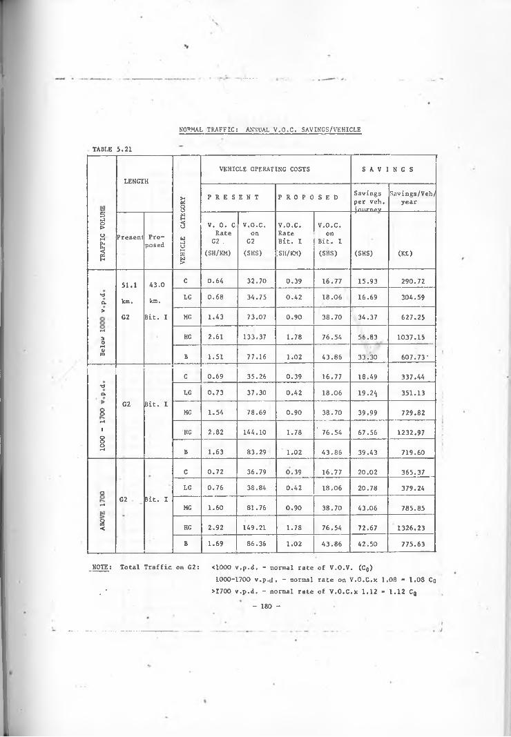
NORMAL TRAFFIC: ANNUAL V.O.C. SAVINGS/VEHICLETABLE 5.21

VEHICLE OPERATING COSTS S A V 1 N G SLENGTH

£8

P R E S E N T P R 0 P 0 S E D Savings per veh.jmirnpv

Savings/Veh/year

TRAFFIC VOLUt

Present Proposed

1MJOMX£

V. 0. C Rate G2 .

(SH/KM)

V.O.C.onG2(SHS)

V.O.C. Rate Bit. I;sh/km)

V.O.C.on

Bit. I (SHS) (SHS) (K£)

51.1 A3.0 c 0.64 32.70 0.39 16.77 15.93 290.72*da km. km. LG 0.68 34.75 0.42 18.06 16.69 304.59> G2 Bit. I MG 1.43 73.07 0.90 38.70 34.37 627.25H>O HG 2.61 133.37 1.78 76.54 56.83 1037.15r-<QJrt B 1.51 77.16 1.02 43.86 33.30 607.73-

C 0.69 35.26 0.39 16.77 18.49 337.44•dp. LG 0.73 37.30 0.42 18.06 19.2^ 351.13

8G2 Bit. I

MG 1.54 78.69 0.90 38.70 39.99 729.82H

1000 - HG 2.82 144.10 1.78 ' 76.54 67.56 1232.97

B 1.63 83.29 1.02 43.86 39.43 719.60

C 0.72 36.79 0.39 16.77 20.02 365.37

O LG 0.76 38.84 0.42 18.06 20.78 379.24H G2 . Bit. I

MG 1.60 81.76 0.90 38.70 43.06 785.85

HG 2.92 149.21 1.78 76.54 72.67 1326.231

B 1.69 86.36 1.02 43.86 42.50 775.63

NOTE; Total Traffic on G2: <1000 .v.p.d. - normal rate of V.O.V. (Cj)1000-1700 v.p.d. - normal rate on V.O.C.x 1.08 “ 1.08 Co

. ' >1700 v.p.d. - normal rate of V.O.C.x 1.12 » 1.12 Cq- 180 -

BENEFITSNORMAL AND GENERATED TRAFFIC: TOTAL V.O.C. SAVINGS

TABLE 5.22 IN K£'OOO'

m* I

NORMAL TRAFFIC GENERATED TRAFFIC •

aR C LG MG HG B C LG MG HG B TOTAL

1974

1975

1976

1977 33.14 39.25 34.50 1.04 9.72 1.60 1.98 1.88 - 0.61 123.7C

1978 36.92 44.17 37.64 2.07 10.94 2.76 3.35 2.82 0.52 0.91 142.1C

1979 41.57 49.39 41.40 2.07 11.55 4.22 4.87 4.08 0.52 1.22 160.87

1980 46.52 55.44 45.79 2.07 12.76 4.65 5.48 4.39 0.52 1.22 178.84

1981 52.04 61.83 50.18 2.07 13.98 5.23 6.09 5.02 0.52 1 198.46

1982 57.27 68.23 54.57 3.11 15.19 5.81 6.70 5.33 0.52 1.52 218.2!

1983 63.09 74.93 59.59 3.11 17.02 6.41 7.46 5.96 1.04 1.82 240.4:

1984 69.19 82.57 63.96 3.11 18.23 6.98 8.07 6.27 1.04 1.82 261.2!

1985 76.17 90.77 70.86 4.15 20.06 7.70 8.99 6.90 1.04 2.13 288.7!

1986 83.73 99.91 77.1! 4.1! 21.86 8.58 9.90 7.53 1.04 2.13 316.OC

1987 91.2S108.71 83.42 4.1! 23.7C 9.30 10.66 8.15 1.04 2.43 342.86

1988 99.72118.4! 89.7( 5.19 25.52 10.81 11.73 8.75 1.56 2.73 373.66

1989 125.8"148.86113.12 6.1C 32.36 12.82 14.7! 10.95 1.85 3.24 4 7 0.o:

1990 137.34162.22121.86 7.4C 35.26 14.06 15.96 12.04 1.85 3.60 5 1 1.5:

1991 149.8 176.9"132.1C 7.4C 38.1 15.16 17.36 13.14 1.85 3.96 555.96

1992 163.32192.77142.31 8.63 41.02 16.5! 18.96 13.87 2.47 4.32 604.2C

1993 177.82210.32153.9! 8.63 44.6i 18.0! 20.72 14.96 2.47 4.68 656.26

1994 1 9 4.o:229.2!166.4C 9.86 48.2: 19.77 22.6! 16.42 2.47 5.04 714.11

1995 211.2*249.6.179.57 11.1C 51.8 21.42 24.56 17.52 3.08 5.40 775.3!

- 1996 1■»----

249.5.293.91208.2! 11.97 60.56 25.3! 29.01 20.43 3.32 6.21 908.51- 181 -

i

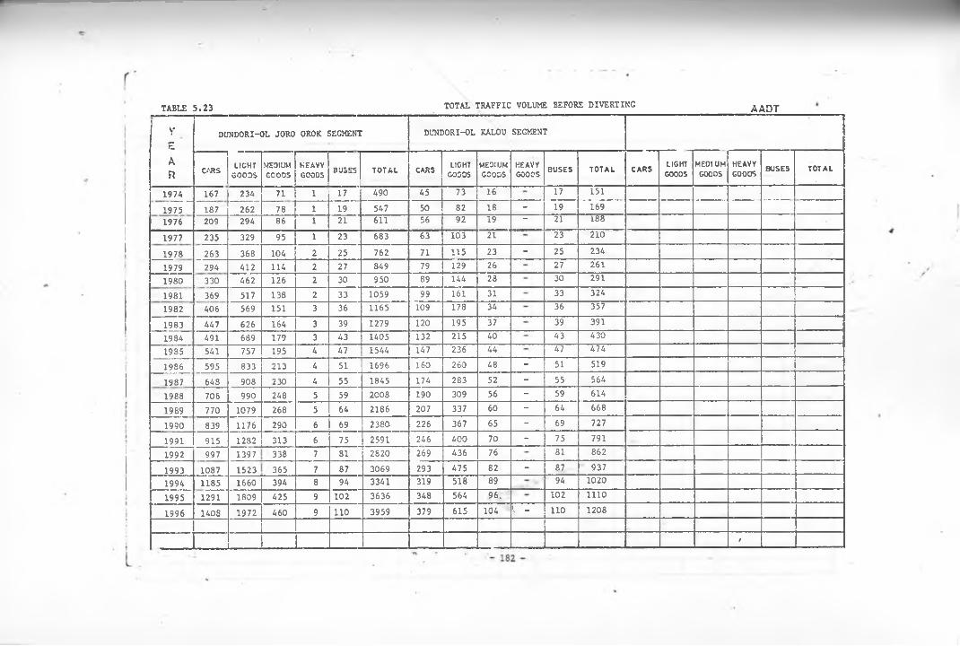
TABLE 5.23 TOTAL TRAFFIC VOLUME BEFORE DIVERTING AADTVEAn

DUNDORI-OL JORO OROK SEGMENT DUNDORI-OL KALOU SEGMENT

CARS LIGHTGOODS

MEDIUMGOODS

H EAVYGOODS BUSES T O T A L CARS

LIGHTGOODS

MEDIUMGOODS

HEAVYGOODS B U SE S T O T A L C A R S

LIGHT

GOODSM EDIUMGOODS

HEAVYGOODS

BUSES TO TAL

1974 167 234 71 i 17 490 45 73 16 17 1511975 187 262 78 i 19 547 50 82 18 - 19 1691976 209 294 86 i 21 611 56 92 19 “ 21 1881977 235 329 95 i 23 683 63 103 21 23 2101978 263 368 104 2 25 762 71 115 23 - 25 2341979 294 412 114 2 27 849 79 129 26 27 2611980 330 462 126 2 30 950 89 144 28 30 2911981 369 517 138 2 33 1059 99 161 31 33 3241982 406 569 151 3 36 1165 109 178 34 36 3571983 447 626 164 3 39 1279 120 195 37 39 3911984 491 689 179 3 43 1405 132 215 40 43 4301985 541 757 195 4 47 1544 147 236 44 47 4741986 595 833 213 4 51 1696 160 260 48 - 51 5191987 648 908 230 4 55 1845 174 283 52 - 55 5641988 706 990 248 5 59 2008 190 309 56 - 59 6141989 770 1079 268 5 64 2186 207 337 60 - 64 6681990 839 1176 290 6 69 2380 226 367 65 - 69 7271991 915 1282 313 6 75 2591 246 400 70 - 75 7911992 997 1397 338 7 81 2820 269 436 76 81 8621993 1087 1523 365 7 87 3069 293 475 82 - 87 9371994 1185 1660 394 8 94 3341 319 518 89 94 10201995 1291 1809 425 9 102 3636 348 564 96. 102 11101996 1408 1972 460 9 110 3959 379 615 104 1 - 110 1208

/

EXPECTED DIVERTED TRAFFICTABLE 5.24 _____________________________________ AADT

YEAR

DUNDORI- OL JORO OROK. DUNDORI - OL KALOU C I L G I L

CARS LIGHTGOODS

MEDIUMGOODS

HEAVYGOODS 9USES TOTAL CARS LIGHT

GOODSMEDIUMGOODS

HEAVYGOODS BUSES TOTAL CARS LIGHT

GOODSMEDIUMGOODS

HEAVYGOODS BUSES TOTAL

1974 53 45 21 - 8 — m — 28 ii i - - 40 19 9 6 - - 341975 59 50 23 - 9 141 31 12 i - - 44 21 10 7 - - 381976 66 55 25 - 10 157 35 14 i - - 50 24 11 7 - - • 4219771978

74 63 28 - 11 176 39 15 i - - 55 27 13 8 - - . 48■83 71 31 - 12 197 44 17 i - - 62 30 14 9 - - • 53

1979 93 79 34 - 13 219 49 19 2 - - 70 33 16 10 - 591980 105

11789 37 - 14 245 55 22 2 - - 79 38 18 11 - - 67

1981 99 • 41 - 16 273 62 24 2 - - 88 42 20 12 - - 741982 129 109 45 - 17 300 68 27 2 - - 97 46 22 13 - - 811983 142 120 49 - 19 330 75 29 2 - - 106 51 24 14 - - 891984 156 132 53 - 20 361 82 32 3 - - 117 56 26 15 - - 971985 172 146 58 - 22 .398 91 36 3 - - 130 61 29 17 - - 1071986 189 160 63 - 24 436 100 39 3 - - 142 68 32 18 - - 11819S71988

206 175 68 - 26 475 109 43 3 - - 155 74 35 19 - - 128224 190 73 - 28 515 118 47 3 - - 168 80 38 21 - - 139

1989 244 207 79 - 30 560 129 51 4 - - 184 88 41 23 - - 1521990 266 226 86 - 33 611 141 55 4 - - 200 95 45 24 - - 1641991 290 247 93 - 35 665 153 60 4 - - 217 104 49 26 - - 1791992 316 269 100 - 38 723 167 66 5 - 238 113 54 29 - - 1961993 345 293 108 - 41 787 182 72 5 1 _ - 259 124 59 31 - - .2141994 376 319 117 - 44 856 199 78 6 - - 283 135 64 33 - - 2321995 410 348 126 - 48 932 217 85 6 - - 308 147 70 36 - - 2531996 447 379 136 - 52 1014 236 93 6 - - 335 160 76 39 - - 275

1- 183

184

■

r~Above 1700 v .p . d • 1000-1700 v . p .d Below 1000 \ •p- . T r a f f i c Volume

O W wH* COa o

to CO H* CO *"0 t

ro r- C. rt NJ • n 2■f O, H NOM h-M M M a 1 GCO CD CO Cd is ta N-* •o

M M* H. CO CDO + Hro <D 4S

MM M H-r MJ! HMlJ

S3 - r o td EG o VEHICLEto O 0 O O o o o :d 03O § r«o CATEG08Y

-

o o o o N- H* o o^ to 5*5 <CD H- W ^o* rt ft o

►-* VO o is is vo o X* O t—* vO 8 X-to co o ■1 Co CO CO o SJ CD CO CO a m^ M

CO W to S3NO >—* c O M NO *-• o o r-* NJ t-* o o cr o p

VO O' 00 c_n "0 O' CD O' is O' O' « CD MVO NJ O O' NO CO ro X' CO 'O *•* f-4 CO 00 3 "3 M n

w CO r*(-* * ►-* S-* CO O' CO t-* h-1 /-n rt w piis CO Co X* is to CD is **J is CO CD

o VO O vO CD O to O' vo cn r-4 r>ro 00 O O is NO CO O O X' NJ 00 o o H

o. <CO is 00 X' NO is is ro *—* CO O _CO 00 NO f—* VO CO O' NO O CD co co o «n p

o *-• VO O CD O' CD h-* CD COx* 00 ro Co is CO O' N-* CD X' o NJ vo is CO pi

(-•00 Co 00 CO CO is CO CO CD X' • 1 CO CO &00 ro h-* CO O' O' VO VO • 1 CD CO NJ O' O' 3^ rt O

w O • • H >ro co CD O' -o O' ' -O S-4 VO CO s-* NJ v^ro m o

f:.

ON O' NO Ol 00 CD X- »-* CD CO NO O vo

CO N**<3

32>—* H-* O o t~* O o N-* 1-* o o o* rt POH-* vO o is vo o X* is h-* vO o is is

CO CO o to CO CO o '-J CD CO CO O CD H *■ - ■— <-> to C? <

o O O o o o »— 1 t-1 O o o CO H* P •o • vo X* o "O vo is o '•J vo X' CO •NO CD O NO vo NO 00 o NO vo NO CD o NJ If M rd o

»-* N-* H-* C-* NJ N-* O' • -S td < oVO CD sj O' vo Cn -O O' -O vo CD vo CJ* rt O o o CO

is is is i> X- CO cn • p • rdO ro o is CO o NO O X* CO o NJ oO to

^ td< COis 'O »—• N-* X* •vl CO »-*• (-* X- CO s-< ►-* co f-

CO O' CO 00 O' ! CO O' 00 oo O' CO O' CO oo O' (A • S b td00 to ■*s| b CD o CD CD " 0 o S - ' M

oO ' X** O O ' O ' o O ' H O ' X* o O '

t-* I-* to Cd <3O ' O CD NO NO O ' O CD ro NO O ' o CD NJ ro

co ! CO CDp * - •

*-• t—• CO NO NJ t—* COi cn OO ' O ' O O ° ! O ' O ' o O o O ' O ' o o o

M

+

'U COis Y-> ►“ * is >-• NJ CO ro I—* V-*

t o

£•vj O ' CO NO C-n ro c-n NO NJ N-* O ' NO o o CO

D* c H*o X> VO vo C CD O ' NO CD CD cn <3 3

o o NO CD CD vO 00 CD a O ' X* vo X- •vj Sot o

x^ X* •vj X" NO CO O' X' »-*VO CO O ■p' CO O ' oo O ' NO NO VO O ' o vo 3- U00 VO o r-* O' CD x« sj CD O CO CD O' ro s: h jNO CD is 00 CD ►-* CO CO CO is vO O' * J «] VO

o NO_____L

CO VO CD VO 1i

u o•_____ I ____ i I ___ ___ ___ 1 1___L

H*>

NH

9*9*

9661 - m i 9861 - 1861 086i - ue\

313IH3A/S OK

I A VS

"0

'0‘A

'IVflX

KV

DIVERTED TRAFFIC: DUNDORI-OL KALOO ~ ACTUAL V.O.C. SAVINGS/VEHICLE

TABLE 5.26

VEHICLE..OPERATING COSTS S A V I N G SPeriodwhenRates

§•JoL E 8 G 1 H

\ >4 W tcd 8M u j 33 H

£ 5

P R E S E N r PROPOSED Savings Savings/uw

H

PRESENT PROPOSEDV.O.C.RATE

Bit.II (SH/KM)

V.O.C.RATEC2(SH/KM)

V.O.C.on

Bit. II (SHS)

V.O.C.onG2(SHS)

TOTAL V.O.C.

Bit. 11 + G2(SHS)

TOTAL V.O.C. on Bit XI + Bit. I

perVehiclejourney

(SHS)

Vehicle/year

(£)

areApplic

able

56.2 km Bit. II

15.4 km Bit. II

c 0.45 0.64 25.29 14.72 40.01 23.70 16.31 297.66•oO* LG 0.47 0.68 26.41 15.64 42.05 25.30 16.75 305.69

1977 to ..

>O8 r—*>O

+23.0 km

+43.0 km MG 1.00 1.43 56.20 32.89 89.09 54.10 34.99 638.57

G2 Bit. I HG 1.93 2.61 108.47 60.03 168.50 106.26 62.24 1135.88 1993'oCQ B 1.13 . 1.51 63.51 34.73 98.24 61.26 36.98 674.891

Sit. II Bit. IIC 0.45 0.69 25.29 15.87 41.16 23.70 17.46 318.65

*d(X LG 0.47 0.73 26.41 16.79 43.20 25.30 17.90 326.68 19948

+ ♦Bit. I MG 1.00 1.54 56.20 35.42 . 91.62 54.10 37.52 684.74 to

19961O8

HG 1.93 2.82 108.47 64.86 173.33 106.26 67.07 1224.03H

B 1.13 1.63 63.51 37.49 101.00 61.26 39.74 725.26

- 185 -

i

DIVERTED TRAFFIC! GILGILi ANNUAL V.O.C. SAVINGS/VEHICLE

TABLE 5.27

/EHICLEVEHICLE- OPERATING COSTS PER VEHICLE JOURNEY Savings Savings

U S 3 T HP R E S E N T P R 0 P 0 S E D per

VehicleJourney

(SHS)

per

’RESENT PROPOSEDCATEGORY V.O.C.

B?ta.teXI(SH/KM)

V.O.C.on Bit. II(106 Km) (SH/KM)

V.O.C.Rate

Bit.- II (SH/KM)

V.O.C. Rate Bit. I (SHS)

V.O.C.-on Bit. II (15.4 Km) (SHS)

V.O.C. on Bit. I (43.0 Km)(SHS)

TOTAL V.O.C. on Bit II + Bit I . (SHS)

perannum«)

C ' 0.45 47.75 0.45 0.39 6.93 16.77 23.70 24.05 433.91106.1 Km 15.4 Km LG 0.47 49.87 0.47 0.42 7.24 18.06 25.30 24.57 448.40Bit. II Bit. II

KG 1.00 106.10 1.00 0.90 15.40 38.70 54.10 52.00 949.00

43.0 Km HC. 1.93 204.77 1.93 1.78 29.72 76.54 106.26 98.51 1797.81

Bit. I B 1.13 119.89 1.13 1.02 17.40 43.86 61.26 58.63 1070.0<3

V

DIVERTED TRAFFIC: DUNDORI-OL JORO OROK & DUNDORI-OL KALOUTABLE 5.2 8 TOTAL V. 0. C. SAVINGS KE'OOO'

B E N E F I T S

'c i

--- DIVERTED TRAFFICDUNDORI - OL JORO OROK

DIVERT DUNDORI -

ED TRA OL KA1

-FIC.OU

*«_ C LG MG HG B C LG MG HG B TOTAL

197419751976

1977 14.27 12.46 11.39 4.39 11.61 4.59 0.64 - - 59.35

1978 16.01 1 4 .0 : 12.6: - 4.79 13.10 5.20 0.64 - - 66.40

1979 17.94 i5.6: 13.83 5.19 14.59 5.81 1.28 - - 74.27

1980 20.25 17.61 15.05 - 5.59 16.37 6.73 1.28 - - 82.43

1981 25.79 22.31 19.16 - 7.44 18.45 7.34 1.28 - 101.77

1982 28.44 24.57 21.03 7.91 20.24 8.25 1.28 - • . 111.72

1983 31.31 27.05 22.9C 8.84 22.32 8.87 1.28 - - 122.57

1984 34.39 29-75 24.77 9.30 24.41 9.78 1.92 - - 134.37

1985 37.92 32.91 27.11 10.23 27.09 11.00 1.92 - - 148.18

1986 41.67 36.06 29.44 “ 11.16 29.77 11.92 1.92 - - 161.94

1987 48.80 42.32 34.o: - 12.95 32.44 13.14 1.92 - ■ - 185.6C

1988 53.06 45.94 36.51 13.95 35.12 14.37 1.92 - - 200.8S

1989 57.80 50.05 39.5: - 14.95 38.40 15.59 2.55 - - 218.8]

1990 63.01 54.65 43.04 16.44 41.97 16.81 2.55 - - 238.41

1991 68.7C 59.73 46.54 17.44 45.54 18.34 2.55 - - 258.8/

1992 74.86 65.05 50.0 18.93 49.71 20.16 3.19 “ 281.96

1993 8i.7: 70.85 54.05 - 20.43 54.i: 22.01 3.19 - - 306.4:

1994 1|j 89.0/ 77.14 58.55 - 21.92 63.41 25.46 4.11 - 339.61

1995 97a: 84.15 63.05 - 23.92 69.15 27.7] 4.11 - - 369.2:

1996 1105 .89 91.65 68.06 25.91 75.2( 30.36 4.11 401.26- 187 -

k

TABLE 5.29DIVERTED TRAFFIC: CILGIL - TOTAL V.O.C. SAVINGS

KE’OOO'

r r iC |

DIVERTED TRAFFIC CILCIL

AR 1 C LG MG HG B TOTAL C LG MG HG B TOTAL

1974 j1975

1976|

1977 11.85 5.83 7.59 - - 2 5 .2 ;

1978 13.17 6.28 8.54 - - 27.99

1979 14.48 7.17 9.49 - - 31.14

1980 16.68 8.07 10.44 - - 35.19

1981 18.43 8.97 11.39 - - 38.79 *1982 20.19 9.8612.34 - - 42.39

*—

1983 22.38 10.76 13.29 - - 46.43

1984 24.58 11.66 14.24 - - 50.48

1985 26.77 13.0016.13 - - 55.90

1986 29.85 14.35 17.08 - - 61.28

1987 32.48 15.6918.03 - - 66.20

1988 35.11 17.04 19.93 - - 72.08

1989 38.62 18.3821.83 - - 78.83

1990 41.70 20.1822.78 _ _ 84.66

. 1991 45.65 21.97 24.67 _ _ 92.291992 49.60 24.21 27.52 - - 101.33

—

1993 54.42 26.46 29.42 - - 110.30

1994 59.25 28.70 31.32 - - 119.27—

1995 64.52 31.39 34.16 _ 130.071996 70.23 34.03 37.01 - - 141.32

- 188 -

- ’JKDIVERTED TRAFFIC

YEAR

DUNDORI-OL JORO OROK DUNDORI-OL KALOU

CARSLIG H T

GOODS

MEDIUM

GOODS

HEAVY

GOODSBUSES T O T A L CARS

LIGHT

GOO OS

MEDIUMGOODS

HEAVYGOODS

BU S E S T O T A L C A R SLIGHT

GOODS

M E D IU M

GOODS

HEAVY

GOODSBUSES T O T A L

197419751976

.19771978

__13LZ9_19801981 252 418 97 2 17 7861982 277 460 106 3 19 8651983 305 506 115 3 20 949 ---T--1984198519861987 442 733 162 4 29 13701988 482 800 175 5 31 14931989 526 872 189 5 34 162619901991199219931994 120 440 83 94 7371995 131 479 90 - 102 8021996 143 522 98 J

— 110 _2Z3___

UNDIVERTED TRAFFIC: ANNUAL V.O.C. SAVINGS/VEHICLEK£ 'OOO’

TABLE 5.31

0 DUNDORI - OL JORO OROK DUNDORI - OL KALOUm0) LENGTH = 30.2 Km. LENGTH - 23.0 Km.

Total Vol

i

VEHICLE

CATEGOR' V.O.C.

Rate G2(Sh/Km)

Savings per vehicle journey (SH)

Savings per vehicle per annum (£)

V.O.C.RATEG2

(Sh/Km)

Savings Der vehicleiou^fi?)

Savingspervehicle p.a

(£)

C 0.64 1.55 28.29 0.64 1.18 21.54

CO

a .

>LG 0.68 1.64 29.93 0.68 1.25 22.81

00o\H

00 MG 1.43 3.45 62.96 1.43 2.63 48.00

r—<00o\

1O HG 2.61 6.31 115.16 2.61 4.80 87.606r —i

B 1.51 3.65 66.61 1.51 2.78 50.74C 0.64 0.77 14.05 0.64 0.59 10.77

- 1989 LG 0.68 0.82 14.97 0.68 0.63 11.50

8NH MG 1.43 1.73 31.57 1.43 1.31 24.09

1987 U>O

3HG 2.61 3.15 57.49 2.61 2.40 43.80B 1.51 1.82 33.22 1.51 1.39 25.37

NOTE: UNDIVERTED TRAFFIC (V")A. When VT “ 1000 - 1700 v.p.d.

Without situation: V.O.C. “ L x 1.08 Cq x V'. . ( when <1000)

With situation: V.O.C. - L x 1.00 C0 x V; where L . distanceSavings = L x 0.08 Cq x V'

B. When VT > 1700 v.p.d.

Without situation: V.O.C. “ L x 1.12 Cq x V"(When V' > 1000 <With .situation: V.O.C. “ L x 1.08 C0 x V — 1 7 0 0 )

Savings “ L x 0.04 Cq x V"

1994 - 1996

B E N E F I T SUNDIVERTED TRAFFIC: TOTAL V.O.C. SAVINGS

KL'OOO'

TABLE 5.32

Vc

UNDIVERTED TRAFFIC DUNDORI - OL JORO OROK

UNDIVERTED TRAFFIC DUNDORI - OL KALOU

AR C LG MG HG B C LG MG HG B TOTAL

1974

19751976

1977

1978

19791980 s

1981 7.13 12.51 6.11 0.23 1.13 V 27.11

1982 7.84 13.77 6.67 0.35 1.27 * 29.90

1983 8.63 15.14 7.24 0.35 1.33 32.69

19841985 ,

1986

1987 6.21 10.97 5.11 0.23 0.96 23.48

1988 6.77 11.98 5.52 0.29 1.03 25.591989 7.39 13.05 5.97 0.29 1.13 27.83

19901991

1992

19931994 2.58 10.04 3.98 - 8.23 24.83

1995 2.82 10.93 4.32 - 8.94 27.01

1996 3.08 11.91 4.70 - 9.64 129.33191 -

192

TABLE 5 .33JOURNEY TIMES ON VARIOUS ROUTE SEGMENTS

Journev - times (in mins.)• Length

(km) c LG MG HG B

1. NAKURU-BAHATI Bit. II 14.5 Speed 80 70 65 60 65II 10.88 12.43 13.38 14.50 L3. 38

2. BAHATI - T. FALLS, G.2 52.0 It 60 55 50 40 4552.00 56.73 52.40 78.00 i 9.33

». NAKURU - LANET Bit. II 5.2 II 90 70 65 60 653.47 4.46 4.80 5.20 4.80

4. LANET-DUNDORI (Tarmac end) " 15.9 II 80 65 60 55 6011.93 14.68 15 .9C 17.35 15.90

i»5. LANET-DUNDORI (Junction) " 14.9 II 80 65 " 60 55 60

11.18 13.75 14.9C 16.25 14.90

6. DUNDORI-OL JORO OROK G.2 30.2 II 70 60 55 50 5525.89 30.20 32.94 36 . 32.94

7. DUNDORI-OL KALOU G.2 23.0 II 65 60 55 50 55?1.23 23.OC 2 5,09 27.60 25 .09

8. OL KALOU—0 L JORO OROK Bit.II 24.0 •I 90 70 65 60 6516.00 20.57 22. 15 24.00 22.15

9. OL JORO OROK-T.FALLS Bit.II 11.1 •1 QO 70 65 60 657.40 9.51 10.24 11. 1C 10.24

10. NAKURU - GILGIL Bit.II 105.1 II 90 70 65 60 6570.07 90.90 17.02 L 05*10 17.02

11 T.FALLS (edge to town centre)Bit.II 1.0 II 60 55 50 40 451.00 1.09 1.20 1.50 1.33

12. BAHATI-T. FALLS (Proposed Road)Bi t. I 43.0 II 80 65 60 55 6032.25 39.69 43.00 46.91 *3.00

%

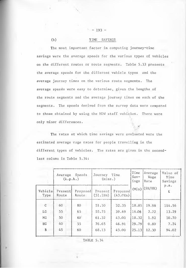
\ 193 -

The most important factor in computing journey-time

savings were the average speeds for the various types of vehicles

on the different routes or route segments. Table 5.33 presents

the average speeds for the different vehicle types and the

average journey times on the various route segments. The

average speeds were easy to determine, given the lengths of

the route segments and the average journey times on each of the

segments. The speeds derived from the survey data were compared

to those obtained by using the MOW staff vehicles. There were

only minor differences.' » ( *

The rates at which time savings were evaluated were the

estimated average vjage rates for people travelling in the

different types of vehicles. The rates are given in the second-

last column in Table 5.34:

(b) TIME SAVINGS

Average(k.p

Speeds.h.)

Journey(mins

Time.)

TimeSavings

(Min)

AverageWage

Rate

(SH/HR)

Value of Time

Savings p.a.

£VehicleType

PresentRoute

ProposedRoute;

Present (51.lKm)

Proposed (43.OKm)

C 60 . 80 51.10 32.35 18.85 19.98 114.56LG : 55 65 55.75 39.69 16.06 2.72 13.29MG 50 : 60' 61.32 43.00 18.32 1.92 10.70HG 40 55 76.65 46.91 29.79 0.80 7.24B 45 60 68.13 43.00 25.13 12.30 94.02

TABLE 5.34

- 194

The time savings were calculated for vehicle trips rather

than for persons travelling in the vehicles. It would have been

an impossible task to estimate the numbers of present and future

road users. On the other hand, the number of vehicle-trips were

readily available once traffic volumes were established. All

those travelling in a vehicle were treated as one vehicle-trip.

The wage rate corresponding to each vehicle type (as shown in

Table 5.34) applies to the occupants in a given vehicle in that

vehicle category as a group constituting a "trip". It is thus

the number of trips, not persons, for which time savings were

estimated. It was thought the other half of the total number\h <

of trips would largely be homeward return journeys on which

time saved would be spent as leisure time.

As in computing VOC savings, only half of the wage rates

was applied in the calculation of the value of time savings for

Generated traffic. The total annual savings for Normal and

Generated traffic are given in Table 5.35.

Time savings for Diverted traffic were arrived at in a

similar manner. The calculations and the resulting values of

expected savings in working time are shown in Tables 5.36, 5.37

and 5.38. No time savings were computed for Undiverted traffic

for the simple reason that it was not anticipated that if the

proposed road were not built:

either (1) that the existing roads would have deteriorated to such an extent,

or (2) that there would have been somuch traffic %

that there would have been significant increases in journey time.

B E N E F I T S

NORMAL AND__GENERATED TRAFFIC: TOTAL TIME SAVINGS

TABLE 5.35 IN Kl'OOO'

w Ic N 0 R M A L T R A F F I C G E N E R A T E D T R A F F I CAR C LG MG HG B C LG MG HG B TOTAL

1974

1975 |1976

1977 13.06 1.71 0.59 0.01 1.50 0.63 0.09 0.03 0.00 0.09 17.71

1978 14.55 1.90 0.64 0.01 1.70 1.09 0.15 0.05 0.00 0.14 20.2:

1979 16.38 2.15 0.71 0.01 1.79 1.66 0.21 0.07 0.00 0.19 23.17

1980 18.33 2.42 0.78 0.01 1.97 1.83 0.24 0.07 0.00 0.19 25.84

1981 20.51 2.70 0.86 0.01 2.16 2.06 0.27 0.09 0.00 0.24 _ 28.9C

1982 22.57 2.98 0.93 0.02 2.35 2.29 0.29 0.09 0.00 0.24 31.76

1983 24.86 3.27 1.02 0.02 2.63 2.52 0.33 0.10 0.01 0.28 35.04

1984 27.27 3.60 1.10 0.02 2.82 2.75 0.35 0.11 0.01 0.28 38.31

1985 30.01 3.96 1.21 0.03 3.10 3.04 0.39 0.12 0.01 0.33 42.20

1986 32.99 4.36 1.32 0.03 3.38 3.38 0.43 0.13 0.01 0.33 46.36

1987 35.97 4.74 1.42 0.03 3.67 3.67 0.47 0.14 0.01 0.38 50.50

1988 39.29 5.17 1.53 0.04 3.95 4.01 0.51 0.15 0.01 0.42 55.08

1989 42.73 5.63 1.66 0.04 4.23 4.35 0.59 0.16 0.01 0.42 59.82

1990 46.63 6.14 1.79 0.04 4.61 4.75 0.60 0.18 0.01 0.47 65.22

1991 50.86 6.70 1.94 0.04 4.98 5.16 0.66 0.19 0.01 0.52 71.06

1992 55.45 7.30 2.09 0.05 5.36 5.61 0.72 0.20 0.01 0.56 77.35

1993 60.37 7.96 2.26 0.05 5.83 6.13 0.78 0.22 0.01 0.61 84.22

1994 65.87 8.68 2.44 0.06 6.30 6.70 0.86 0.24 0.01 0.66 91.82

1995 71.71 9.45 2.63 0.07 6.77 7.27 0.93 0.26 0.02 0.71 99.82

1996 78.24 ,10.30 2.84 0.07 7.33 7-26, 1.02 0.28 H-Q2- 0.21. loa-ai.195

T I M E S A V I N G S

DIVERTED TRAFFIC: ANNUAL TIME SAVINGS/VEHICLE TABLt 5.36 ' 1 r 1 ------ ■ ■DUNDORI - OL JORO OROK

Present Proposed VF.HICI.lCATE-GORY

Average Journey time (in mins.)

Timesavings

Averagewagerate^Sh/Hr)

Time savings per

vehicle p.a.(£)

33.2 Km Bit.II

30.2 Km G2

15.4 Km Bit. II

43.0 Km Bit. I

PRESENT PROPOSED ‘(in mins)

C 49.69 44.03 5.66 19.98 34.40LG 59.94 53.10 6.84 2.72 5.66

MG 65.08 57.46 7.62 1.92 4.45HG 71.39 62.76 8.63 0.80 2.10

B 65.21 57.58 7.63 12.30 28.55

i j ! !DUNDORI - OL KALOU 1

PRESENT

56.2 Kra Bit.II

23.0 Kra G2

PROPOSED

-do -

C 60.28 44.03 16.25 19.98 98.76

LG 72.38 53.10 19.28 2.72 15.95MG 78.38 57.46 20.92 1.92 12.22

HG 85.65 62.76 22.89 0.80 5.57B 78.51 57.58 20.93 12.30 78.30

GILGIL - OL JORO OROK 1j

PRESENT PROPOSED C 71.07 44.03 27.04 19.98 164.33

106.1 Km

Bit. II- do -

LG 91.18 53.10 38.08 2.72 31.50

MG 98.22 57.46 40.76 1.92 23.80

HG 106.60 62.76 43.84 0.80 10.67

B 98.35 57.58 40.77 12.30 152.53

DIVERTED TRAFFIC: DUNDORI-OL JORO OROK & DUNDORI-OL KALOU TOTAL TIME SAVINGS IN KI'OOO'

B E N E F I T S

mc

DIVERTED TRAFFIC DUNDORI- OL JORO OROK

DIVERTEDDUNDORI

TRAFFIC - OL KALOU

AR C LG MG HG B C LG MG HG B TOTAL

19741975

1976

1977 2.55 0.36 0.12 - 0.31 3.85 0.24 0.01 - - 7.44

1978 2.86 0.40 0.14 - 0.34 4.35 0.27 0.01 - - 8.37

1979 3.20 0.45 0.15 - 0.37 4.84 0.30 0.02 - - 9.33

1980 3.61 0.50 0.16 - 0.40 5.43 0.35 0.02 - - 10.47

1981 4.02 '0.56 0.18 - 0.46 6.12 0.38 0.02 - - y . 11.74

1982 4.44 0.62 0.20 - 0.49 6.72 0.43 0.02 - -

■' **

12.921983 4.88 0.68 0.22 - 0.54 7.41 0.46 0.02 - - 14.21

1984 5.37 0.75 0.24 - 0.57 8.10 0.51 0.04 - - 15.58

1985 5.92 0.83 0.26 - 0.63 8.99 0.57 0.04 - - 17.24

1986 6.50 0.91 0.28 - 0.69 9.88 0.62 0.04 - - 18.92

1987 7.09 0.99 0.30 - 0.74 10.76 0.69 0.04 - ■ - 20.61

1988 7.71 1.08 0.32 - 0.80 11.65 0.75 0.04 - - 22.35

1989 8.39 1.17 0.35 - 0.86 12.74 0.81 0.05 - - 24.37

1990 9.15 1.28 0.38 - 0.94 13.93 0.88 0.05 - - 26.61

1991 9.98 1.40 0.41 _ 1.00 15.11 0.96 0.05 - - 28.91

1992 10.87 1.52 0.45 - 1.08 16.49 1.05 0.06 - 31.52

1993 11.87 1.66 0.48 - 1.17 17.97 1.15 0.07 - - 34.36

1994 12.93 1.81 0.52 - 1.26 19.65 1.24 0.07 - - 37.48

1995 14.10 1.97 0.56 - 1.37 21.43 1.36 0.07 - - 40.86

1996 15.38 2.15 0.61 - 1.48 23.31 1.48 0.07 - - 44.48- 197 -

v

*

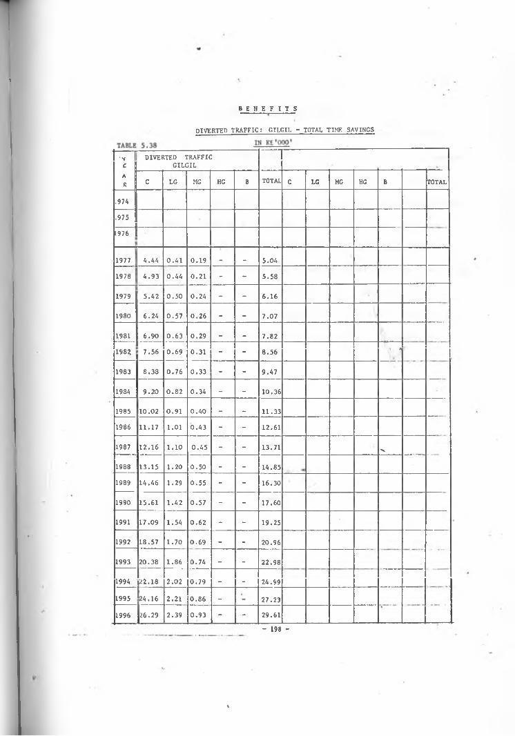
1

B E N E F I T S

DIVERTED TRAFFIC: GILCIL - TOTAL TIME SAVINGS

•V 1 c 1!

DIVERTED TRAFFIC GILGIL

AR C LG MG HG B T0TA1 C LG MG HG B TOTAL

L 9 74L975L976

1977 4.44 0.41 0.19 - - 5.041978 4.93 0.44 0.21 - - 5.58

1979 5.42 0.50 0.24 - - 6.16

1980 6.24 0.57 0.26 - - 7.07

1981 6.90 0.63 0.29 - - 7.821982 7.56 0.69 0.31 - - 8.56 \ A

1983 8.38 0.76 0.33 - - 9.47

1984 9.20 0.82 0.34 - - 10.36

1985 10.02 0.91 0.40 _ _ 11.331986 11.17 1.01 0.43 - - 12.61

1987 12.16 1.10 0.45 - - 13.71 ■v

1988 13.15 1.20 0.50 - - 14.851989 14.46 1.29 0.55 - - 16.30

1990 15.61 1.42 0.57 - - 17.60

1991 17.09 1.54 0.62 - - 19.25

1992 18.57 1.70 0.69 - - 20.96

1993 20.38 1.86 0.74 - - 22.98

1994 22.18 2.02 0.79 _ _ 24.991995 24.16 2.21 0.86 - 27.231996 26.29 2.39 0.93 - - 29.61

- 198 -

t

- 199 -

The savings in annual costs of maintaining the present

Bahati-T. Falls road were obtained by subtracting the estimated

annual cost of maintaining the proposed tarmac road from the

cost that would have been incurred to maintain the present road

if the proposed one were not built. The basic calculations

were given in the section dealing with the computation of

project costs. The estimated maintenance costs for the existing

and proposed roads are given in Table 5.18. The resulting

savings in maintenance costs are as shown in Table 5.40 which

also summarizes the values of the three principal benefits.

(c) MAINTENANCE COST SAVINGS

%

SUMMARY OF V. 0. C. SAVINGS AND TIME SAVINGS

YEAR

N O R M A L G E N E R A T E D

DIVERTED AND UNDIVERTED. DUNDORI-OL JORO

OROK

DIVERTED AND UNDIVERTED

DUNDORI-OL KALOU DIVERTED - GILGILTOTAL V.O.C. AND TIME SAVINGS

V.O. C. SAVINGS

TIMESAVINGS

V.O.C.SAVINGS

TIMESAVINGS

V.O.C.SAVINGS

TIMESAVINGS

V.O.C.SAVINGS

TIMESAVINGS

V.O.C.SAVINGS

TIMESAVINGS

V.O.C.SAVINGS

TIMESAVINGS

1977 117.69 16.87 6.07 0.84 42.51 3.34 16.84 4.10 25.21 5 .04 208.35 30.191978 131.74 18.80 10.36 1.43 47.46 3.74 18.94 4.63 27.99 5.58 236.49 34.181979 145.93 21.04 14.91 2.13 52.59 4.17 21.68 5.16 31.14 6.16 266.25 38.661980 162.58 23.51 16.26 2.33 58.05 4.67 24.38 5.80 35.19 7.07 296.46 417181981 180.10 26.24 18.38 2.66 101.81 5.22 27.07 6.52 38.79 TT52 366.13 U 48.461982 198.37 28.85 19.88 2.91 111.85 5.75 29.77 7.17 42.39 8.56 402.26 53.24lofn 217.74 31.80 22.68 3.24 122.79 6.32 32.47 7.89 46.43 9.47 442.11 58.721984 237.05 34.81 24.18 3.50 98.21 6.93 36.11 8.65 50.48 10.36 446.03 64.251985 262.03 38.31 26.76 3.89 103.17 7.64 40.01 9.60 55.90 11.33 492.87 70.771986 ■ 286.82 42.08 29.18 4.28 118.33 8.38 43.61 10.54 61.28 12.61 539.22 77.891987 311.30 45.83 31.58 4.67 161.58 9.12 47.50 11.49 66.20 13.71 618.16 '84.82'1988 338.62 49.98 34.98 5.10 175.07 9.91 51.41 12.44 72.08 14.85 672.16 92.281989 426.41 54.29 43.61 5.53 190.16 10.77 56.54 13.60 78.83 16.36 795T55 100.491990 464.10 59.21 47.47 6.01 177.14 11.75 61.33 14.86 84.66 17.60 834.70 109.431991 504.43 64.52 51.51 6.54 192.41 12.79 66.43 16.12 92.29 19.25 907.07 119.231992 548.05 70.25 56.15 7.10 208.88 13«?2 73.08 17.60 101.33 “20796 "937759 “TZ97B31993 595.40 76.47 60.88 7.75 227.06 15.18 79.37 19.18 110.30 22.98 L073.01 141.561994 647.79 83.35 66.32 8.47 246.68 16.52 117.83 20.96 119.27 24.99 L197.89 154.291995 703.34 90.63 72.01 9.19 268.24 18.00 128.04 22.86 130.07 27.23 L301.70 167.911996 824.15 98.78 84.36 10.03 291.51 19.62 139.02 24.86 141.32 29.61 L480.36 182.90

200 -

S U M M A R Y O F B E N E F I T S

IN Kt'OOO'TABLE 5.40

YEAR

VEHICLEOPERATINGCOSTSAVINGS

TIMESAVINGS

MAINTENANCECOSTSAVINGS

TOTAL

BENEFITS

1977 208.36 30.19 - 258.571478 236.49 34.18 3.34 274.01

1979 266.25 38.66 3.34 308.25

1980 296.46 43.38 19.58 359.421981 366.15 48.46 3.34 417.95

1982 402.26 53.24 -15.79 439.71

1983 442.11 58.72 19.58 520.41

1984 446.03 64.25 3.34 513.621985 492.87 70.77 3.34 566.98

1986 539.22 77.89 19.58 636.69

1987 618.16 84.82 3.34 706.321988 672.16 92.28 -15.79 748.65

1989 795.55 100.49 19.58 915.62

1990 834.70 109.43 3.34 947.47

1991 | 907.07 119.22 3.34 1029.63

1992 | 987.49 129.83 19.58 1136.90

1993 i 1073.01 141.56 3.34 1217.91

1994 ! 1197.89 i 154.29 -15.79 1336.39

1935 j 1301.79 167.91 19.58 1499.291996 I 1480.36 ii 182.90 j 3.34 1666.60

i i i I- 201 -

i

>»

COST-BENEFIT ANALYSIS

TABLE 5.41 Kt'OOO'

Y C O S T S B E N E F I T SEAR

TOTALCOSTS

Discounted @ 14%

Discounted @ 171

Discounted @ 181

TOTALBENEFITS

Discounted @ 14%

Discounted @ 17%

Discounted @18%

1975 944.50 947.50 947.50 947.501976 1235.88 1084.11 1056.31 1047.41

1977 2;i .56 186.65 177.19 174.21 238.57 183.58 174.28 171.34

1978 4.79 3.23 2.99 2.92 274.01 184.96 171.09 166.76

1979 4.79 2.84 2.56 2.47 308.25 182.51 164.51 159.83

1980 4.79 . 2.49 2.18 2.09 359.42 186.68 163.93 157.101981 4.79 2.18 1.87 1.77 417.95 190.42 162.92 154.81

1982 23.92 9.56 7.97 7.51 439.71 175.71 146.51 138.02

1983 4.79 1.68 1.36 1.27 520.41 182.46 148.21 138.43

1984 4.79 1.47 1.17 1.08 513.62 157.94 125.02 115.82

1985 4.79 1.29 1.00 0.92 566.98 152.91 117.93 108.35 1

1986 4.79 1.13 0.85 0.78 636.69 150.64 113.20 103.08 |-1987 4.79 0.99 0.73 0.66 706.32 146.63 107.36 96.91

1988 23.92 4.36 3.11 2.78 748.65 136.33 97.25 87.07

L989 4.79 0.76 0.53 0.47 915.62 146.22 101.63 90.19

jl990 4.79 0.67' 0.45 0.40 947.47 132.74 89.91 79.11

jl991 4.79 0.59 0.39 0.34 1029.63 126.54 83.50 72.98i

|l992 4.79 0.52 0.33 0.29 1136.90 122.56 78.79 68.21

19931

4.79 0.45 0.28 0.24 1217.91 115.21 72.10 61.87

1994 23.92 1.98 1.21 1.03 1336.39 110.79 67.62 57.60

1995 4.79 0.35 0.21 0.17 1499.29 108.42 64.49 54.36

V»5

Vi O 4.79 0.31 0.18 ‘ 0.15 166.60 106.33 61.66 51.50

2255.11 2210.37 2196.46 2999.58 2311.91 2133.34- 202 - __ r*-

*#

v .

S E N S I T 1 V I T Y I N A I Y S I S : I

TABLE 5.42 " K£'000'Y C 0 S T S x 1 . 1 0 B E N E F I T SEAR

Discounted

6 14%Discoun

ted @ 16%

Discounted

@ 17%)iscoun- ted

@ 14%Discoun

ted @ 16%

Discounted

@ 17%1975 1042.25 1042.25 1042.25

1976 1192.53 1172.00 1161.94

1977 205.32 198.30 194.91 183.58 177.31 174.28

1978 3.56 3.38 3.29 184;96 175.56 171.09

1979 3.12 2.91 2.81 182.51 170.25 164.51

1980 . 2.74 2.51 2.40 186.68 171.11 163.93

1981 2.40 2.16 2.05 190.42 171.53 162.92

1982 10.51 9.31 8.77 175.71 155.57 146.51

1983 1.85 1.61 1.50 . 182.46 158.73 148.21

1984 1.62 1.39 1.28 157.94 135.08 125.02

1985 1.42 1.19 1.10 152.91 128.53 177.93

1986 1.25 1.03 0.94 150.64 124.41 113.20

1987 1.09 0.89 0.80 146.63 119.01 107.36

1988 4.79 3.82 3.42 136.33 108.70 97.25

1989 0.84 0.66 0.58 146.22 114.64 101.63

1990 0.74 0.57 0.50 132.74 102.23 89.91

1991 0.65 0.49 0.43 126.54 95.76 83.50

1992 0.57 0.42 0.37 122.56 91.18 78.79

1993 0.50 0.36 0.31 115.21 81.16 72.10

1994 2.18 1.57 1.33 110.79 79.65 67.62

1995 0.38 0.27 0.23 108.42 76.55 64.49

1996 0.34 0.23 0.19 106.33 73.83 61.66

2480.65 2447.32 2431.40 - 203 - 2999.58 2510.79 2311.91

■*

\

S E N S I T I V I T Y A N A L Y S I S : II

TABLE 5.43 Kt'OOO'

Y C 0 S T S B E N E ] ' I T S x 0 . 90

E Discoun- Discoun- Discoun- Discoun- Discoun- Discoun-ted ted ted ted ted ted

AR 0 142 0 162 0 172 0 142 0 162 0 172

1975 947.50 947.50 947.50

1976 1084.11 1065.45 1056.31

1977 186.65 180.27 177.19 165.22 159.57 156.85

1978 3.23 3.09 2.99 166.46 158.00 153.98

1979 2.84 2.65 2.56 164.27 153.22 148.061980 . 2.49 2.28 2.18 168.02 154.00 147.54

1981 2.18 1.97 1.87 171.38 154.38 146.631982 9.56 8.46 7.97 158.14 140.01 131.86

1983 1.68 1.46 1.36 164.21 142.82 , v 133.39

1984 1.47 1.26 1.17 142.14 121.57 112.51

1985 1.29 1.09L 1.00 137.62 115.68 106.14

1986 1.13 0.94 0.85 135.58 111.96 101.881987 0.99 0.81 *0.73 - 131.97 107.11 96.62

1988 4.36 3.47 3.11 122.70 97.83 87.53

1989 0.76 0.60 0.53 131.60 103.17 91.47

1990 0.67 0.52 0.45 119.47 92.00 80.92

1991 0.59 0.45 0.39 113.89 86.18 75.151992 0.52 0.38 0.33 110.30 82.06 70.90

1993 0.45 0.33 0.28 103.69 75.74 64.89

1994 1.98 1.43 1.21 99.71 71.68 60.861995 0.35 0.25 0.21 97.58 68.89 58.04

1996 0.31 0.21 0.18 95.70 66.45 55.50

2255.11 2224.87 2210.37 - 204 - 2699.65 2262.65 2090.73

TABLE 5.44S E N S I T I V I T Y A N A L Y S I S : III

KI'OOO'

Y C O S T S x 1 1 0 B E N E F I T S x 0 . 9 0

EAR

Discounted

0 14%Discoun

ted @ 16%

Discounted

@ 17%Discoun

ted 0 14%

Discounted

0 16%Discoun

ted 0 17%

1975 1042.25 1042.25 1042.25

1976 1192.53 1172.00 1161.94

1977 205.32 198.30 194.91 165.22 159.57 156.85

1978 3.56 3.38 3.29 166.46 158.00 153.98

1979 3.12 2.91 2.81 164.27 153.22 148.06

1980 2.74 2.51 2.40 168.02 154.00 147.54

1981 2.40 2.16 2.05 171.38 154.38 146.63

1982 10.51 9.31 8.77 158.14 140.01 131.86

1983 1.85 1.61 1.50 164.21 142.85 133.39

1984 1.62 1.39 1.28 142.14 121.57 112.51

1985 1.42 1.19 1.10 137.62 115.68 106.14

1986 1.25 1.03 a.94 135.58 111.96 101.88.

1987 1.09 0.89 0.80 131.97 107.11 96.62

1988 4.79 3.82 3.42 122.70 97.83 87.53

1989 0.84 0.66 0.58 131.60 103.17 91.47

1990 0.74 0.57 0.50 119.47 92.00 80.92

1991 0.65 0.49 0.43 113.89 86.18 75.15

1992 0.57! 0.42 0.37 110.30 82.06 70.91

19931! 0.50 0.36 0.31 103.69 75.74 64.89

1994 : 2 . 1 8 1.57 1.33 99.71 71.68 60.861995 0.38 0.27 0.23 97.58 68.89 58.04

1996 0.34 0.23 0.19 95.70 66.45 55.502480.65 2447.32 2431.40

- 205 -2699.65 2262.35 2090.73

- 206 -

5.33 COMPARING THE COSTS AND BENEFITS

The cost and benefit streams were discounted at 14% to

determine the net present worth (NPV) of the proposed road

project. This discount rate, the Ministry of Finance and

Planning reckons is the opportunity cost of capital in the

public sector in Kenya. At 14% the project has a net social

benefit of some £744,470.

Using the World Bank criterion, the project has an

economic internal rate of return (IRR) of 17.62% and Benefit-

Cost (B/C) ratio of 1.33. On the basis of all the three'V*

criteria the proposed investment is worth undertaking. "Even if

the cut-off rate were set slightly higher - say at 15% the

proposed road project would still be a desirable investment.

The details of the discounted values are given in Table 5.41.

The following computations demonstrate how the above three

indices were derived:

1) Net Present Worth

Benefits and costs discounted - @ 14%

PVji+(B) = 2999.58 where PV^= discounted PV @ 14%

PV14(C) = 2255.11

NPViif . = 744.,47

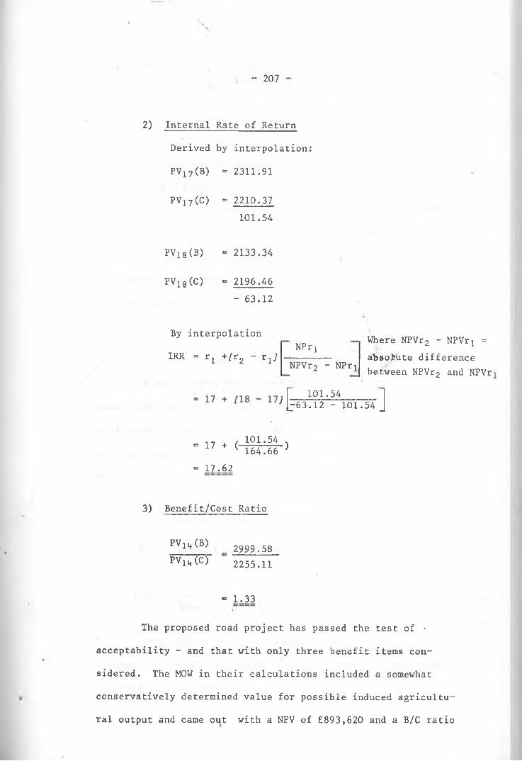
- 207

2) Internal Rate of Return

Derived by interpolation:

p v17(b) = 2311.91

PV17(C) = 2210.37101.54

pvi8(b) = 2133.34

PVi8<C) = 2196.46- 63.12

By

IRR

interpolation

= rl +/’r2 “ ri-7

- 17+0 101.54164.66

NPr i Where NPVr2 - NPVr^ =absolute difference between NPVr2 and NPVrNPVr2 - NPrjL

f 101.54 1J[j63.12 - 101 .54 J

-)

= 17.62

3) Benefit/Cost Ratio

PVllt(B) P V l lt ( C )

2999.582255.11

= 1^33

The proposed road project has passed the test of •

acceptability - and that with only three benefit items con

sidered. The MOW in their calculations included a somewhat

conservatively determined value for possible induced agricultu

ral output and came out with a NPV of £893,620 and a B/C ratio

- 208 -

of 1.41 - both of these at 14%; and an IRR of 18.50%. But the

way the induced agricultural benefit was derived left much to

be desired - and as the above calculations indicate the

inclusion of the value of expected net induced agricultural

output does not materially alter the degree of acceptability

of the proposed road investment. The Ministry made no effort

to estimate the value of possible induced economic activity

in industry or tourism; reductions in potential accidents or

secondary effects.

5.34 SENSITITIVY ANALYSIS

A very simple sensitivity analysis was attempted. It

consisted simply of a consideration of how the economic worth

of the project would be affected if its costs were to rise by

10% and benefits were to fall by 10%. Three possibilities

were considered:

(i) Costs rise by 10% (C x 1.10)Benefits remain unchanged (B = kj)

Cii) Costs remain constant (C = k^)Benefits fall by 10% (B x 0.90)

(iii) Costs rise by 10%Benefits fall by 10%.

The effects of these assumptions on the above three

indices of the economic worth of an investment are summarized

in the following table:

I

- 209 -

Net Present Worth B/CRatio@

14%

IRR

%Costs Benefits @14% @16% @17%

C x 1.10 B = kx 518.93 63.47 -119.49 1.21 16.35

CM

IIu B x 0.90 244.54 37.48 -119.64 1.20 16.24

C x 1.10 B x 0.90 219.00 -184.97 -340.67 1.09 15.02

TABLE 5.45 (a)

The project would definitely be uneconomic if the cut

off rate were as high as 17%. At 16% it would.just be a

marginal project if assumptions (i) and (ii) hold and undesirable

if (iii) holds true. According to the MOW calculations the

project would be rejected if the cut-off rate were 18%, and

only marginal at 17%. The table below shows the effect of

including the agricultural benefit, given the three assumptions:

‘ • Net Present Worth B/C RATIO @14%

IRR

C o s t s Benefits @14% @ 17% %

C x 1.10 B = kj 675.11 26.52 1.28 17.1

C = k2 B x 0.90 591.15 2.25 1.27 17.0

C x 1.10 B x 0.90 392.64 -211.89 1.15 15.9

TABLE 5.45 (b)

Although theoretically more plausible, a more sophisti

cated sensitivity analysis would have been impracticable for

%

- 210

this case study in the light of the paucity of information on

the various aspects of the case study project.

' v

C H A P T E R V I

THEORY AND PRACTICE REVISITED

In this concluding chapter an attempt will be made to

highlight the extent to which the hypothesis made in an earlier

chapter is borne out by what has been presented in the preced

ing four chapters. In the statement of hypothesis it was

suggested that there are two basic sources of cost/benefit

measurement problems. One is the way some of the items of

road project costs and benefits are defined. The second is

in the measurement procedures that have been proposed and used

to date.

The ultimate root cause of both of these problems is

in the nature of the costs and benefits. Project costs in CBA

are Social Opportunity Costs (SOCs). The benefits are in the

nature of Consumers Surplus (CS). Essentially CS is a saving:

that part of the willingness-to-pay that is unrevealed or

unrealized as producer's revenue. The benefits of a road are

thus savings on some items of cost.

6.1 ESTIMATING COSTS

Given the definition of project costs as SOCs the

first problem in measuring them is to identify the best forgone

alternative uses for project inputs. In some cases it will be

- 212 -

relatively easy to locate such uses; in others - and perhaps in

the majority of cases - it will be difficult and largely a

matter of subjective judgement. This point is brought out more

forcefully if one keeps in mind that in fact, CBA, unlike micro-

or macro-economic theory, is Normative Economics. Objectivity

in matters of what should or should not be is very difficult to

establish and maintain because normative issues invariably

involve value judgements. Value, whether in Economics or

in some other sphere of life is a very intricate matter to deal

with. Defined in utilitarian terms, value is intrinsically

immeasurable. And yet it is this very element that ultimately' i i *

must be the criterion to guide choice of the best alternative

uses of economic resources. If the aim in project evaluation

is to determine how best to deploy society's scarce resources

in such a manner as to maximise social benefits - and social

benefits are essentially CS - then indeed strictly speaking,

there can be no objective measurable and verifiable criterion

for selecting the best or next best alternative resource use(s).

This, coupled with the possibility that a resource might have

a large number of alternative uses forms a fairly formidable

factor in the evaluation of alternative resource uses. Moreover,

in dynamic economic circumstances no one use or set of uses can

remain the best or next best at all times. With the shift in

emphasis on what is the next best use of a resource there is

also a change in the opportunity cost value of that resource.

The consequence of this is that it becomes very difficult to

obtain adequate and reliable data for evaluating resource uses.

213 -

The theoretical framework described earlier presented

details of the theoretical proposals on how to measure costs.

The proposals represent what is conceptually plausible. The

case study on the other hand attempted to demonstrate what is

empirically possible. In some cases it seems the gap between

what is conceptually sound and what is feasible in practice is

unbridgeable. Such would seem to be the case with the deter

mination of the opportunity cost of some project inputs. Thus,

as exemplified by the procedure for calculating the shadow

wage rate for unskilled labour in the Little-Mirrlees system,

ultimately the opportunity cost of this category of labour can% «r

not be established solely by means of objective economic

criteria and procedures. The attitude of the government towards

current and future consumption must be taken into account when

calculating this shadow wage rate.

The ideal approach to measuring the costs of a public

sector project would be to estimate the opportunity cost of

each project input separately. This is because the opportunity

cost values of the inputs differ to the extent that their

best alternative uses are not identical.

6.11 CONSTRUCTION EQUIPMENT

The SOC of capital equipment used in road construction

would, in principle, be the reduction (properly adjusted to

reflect social valuation) in the expected market value of the

equipment. In practice not only may it not be possible to

establish correctly the opportunity cost of construction

- 214 -

equipment but also estimates of the reductions in the discounted

values of the equipment may not be - and usually they are not -

available for two possible reasons:

1. To be able to estimate the expected value of a piece of equipment one would need to know firstly the expected economic life of the equipment, and secondly the trends in the price(s) of its output(s). For all that anybody can tell both of these two are anything but simpleto estimate.

2. Then there is the problem of determining the percentage decline in the expected value due to usage of the equipment on a given construction project.

' \ *

This ideal method would obviously be impracticable. The economic

life of equipment is partly a function of physical wear and

tear but largely a function of obsolescence. Whereas the rate

of wear and tear can be estimated with reasonable accuracy,

that of obsolescence - particularly in conditions of rapid

technological changes - is too difficult to gauge. The impli

cation of this must be that it is also just as difficult to

estimate the economic life of the equipment. Consequently,

measuring the value of economic depreciation in the manner

suggested in the theoretical framework is impracticable.

If the construction of a road is awarded to a foreign

contractor the foreign exchange component in the economic depre

ciation of his construction equipment must be shadow-priced.

The shadow-pricing procedure would consist of establishing the

value of what goods and services the domestic economy must forgo%

- 215 -

so as to generate the amount of FE necessary to pay for the

services of the equipment. Assuming economic rationality on

the part of the contractor this amount of FE would at least

be equal to the estimated decline in the expected value of his

equipment.

Thus, bringing the FE element into the evaluation

process does not make any difference to the basic definition

of the social cost value of the services of construction equip

ment. But it does introduce a new problem: that of identifying

the appropriate items which the home economy gives up in order

to earn the FE. There is no label on FE funds to indicate\ V

which sum was earned by which items exported or import items

displaced.

6.12 CONSTRUCTION MATERIALS

The procedure for valuing construction materials will

depend on whether the materials are imported or produced

locally. If they are imported their FE cost would be shadow

priced at the domestic value (gross of any subsidies or net of

all indirect taxes) of the goods exported or imports displaced

to earn it. Locally procured materials would be valued at

their domestic prices - appropriate adjustments being done to

the market values, to take into account the effects of domestic sub

sidies and indirect taxes. Ideally, since most materials are

purchased in markets that are far from being perfectly compe

titive, their market values should also be adjusted for price

distortions arising from market imperfections by valuing them%

- 216 -

at what they would have sold for in a perfectly competitive market.

In practice this is clearly impossible. Perfect competition is

a hypothetical model that so far has only existed in the imagi

nation of economic theorists. Consequently, the project

evaluator must be content with shadow-pricing as the only

feasible way of dealing with price distortions arising from

market imperfections. In the case study the shadow pricing of

construction materials took the form of a 10% indirect tax

deduction from total construction and maintenance costs. But

this adjustment is not good enough because it does not specifi

cally relate to materials. It implies that there was a 10% tax

on all the project input items which of course is not the case.

Only some of these might have duties imposed upon them but it

was difficult to determine the tax rate on each of them. More

over, maintenance costs were estimated and given as lumpsum

amounts: no detailed breakdowns of them such as those shown

in Table 5.15 for construction costs were available to enable

the computation of indirect taxes on each item. Ideally, dis

tortions in the market prices of materials due to monopolistic

influences or other market imperfections should also be removed

from the construction and maintenance costs. However, in the

absence of a criterion for the identification of such distortions

or a procedure for their removal the only adjustment done to

the costs in the case study was the elimination of indirect

taxes. It was assumed there were no subsidies on the materials

or any other input item.

%

- 217 -

6.13 LAND AND LABOUR

The valuation of unskilled labour is a particularly

troublesome exercise whether one adopts the willingness-to-pay

approach or the World Prices method. The services of skilled

(foreign) personnel, under the willingness-to-pay approach

would be valued much in the same way as imported materials.

Locally procured labour services should in principle be valued

at the minimum wage rate(s) the workers would be prepared to

accept.

If this were all that was to be done to establish the\

economic cost of local labour, the main problem would be to

obtain the appropriate amount and quality of information on

the minimum wage rate that workers would accept in order to

take up a job on a road project. Unfortunately, this minimum

wage rate would be a private opportunity cost value and would

have to be translated into a social cost. Most problems

relating to the evaluation of unskilled labour are in this

conversion of private or financial labour costs into social

costs. Little and Mirrlees in their model have proposed a

fairly structured procedure for estimating the shadow wage

rate. But they also recognize the limitation to the procedure

posed by the need to accommodate government policy towards

present and future consumption. Procedural rigor must^ there

fore, give way in the face of this unquantifiable but crucial

consideration in the determination of the shadow wage rate.

%

' - 218 -

The Willingness-to-pay method on the other hand, beyond

stating in general terms that the shadow rate is (or should be)

the minimum rate of remuneration workers would be willing to

accept, provides no definite method of how this minimum

acceptable rate is to be determined. There is only one way to

go about this: empirical investigation.

The estimation of the economic value of land is similar

to that of unskilled labour. Price ceilings in the land market

imposed by the Governmnet as well as socio-political factors

militate against "free" land transactions in this country. This

means that land market prices fail to reflect the trfle social

value of land. The land that will be acquired from farmers for

the construction of the proposed Bahati-T. Falls road will

probably be paid for at Government land rates which do not even

reflect market prices for land, let alone the social cost value

of it. So even though the cost of land will be an insignificant

proportion of the total construction costs for the road the

fact still remains that insignificant proportion will be a poor

approximation of the social value of the land. In principle,

the social value of the land would be the minimum price land-

owners would accept or conversely the maximum price prospective

land buyers would be willing to pay for the land. But given

Government price controls and social influences on the land

market, market land prices in particular areas would not

be reliable indicators of the value of land to the economy. In

the case study the cost of land was not treated as a separate

- 219 -

item for the simple reason that it was not considered to be

large enough to merit such treatment.

The effects of Government land policy appear to be

confined to matters of price control and, unlike the case of

unskilled labour, such policy would not be as an important

consideration in the definition and computation of the shadow

price of land as it is in the calculation of the shadow wage

rate for unskilled labour (especially in the Little-Mirrlees

system). Fortunately, under the willingness-to-pay approach,

apart from adjustments for taxes or subsidies (if any) on landfit

transactions, no other adjustments would be necessary.

6.14 ADVERSE SPILLOVERS

The problems associated with the evaluation of external

effects were set out in detail in preceding chapters. Perhaps

the only significant one of them would be increased risk of

accidents on the new road. The other ones would probably not

be large enough to justify undertaking the complicated evalua

tion process required for them. It should be noted here in

passing that the MOW does not normally bother measuring spill

over effects whether important or unimportant. The main reason

seems to be that they do,not have staff competent enough to do

this. They do, however, acknowledge the substantial cost to

the country resulting from road accidents.

Spillover effects are perhaps the best of project

effects for which the gap between the measurement procedures%

- 2 2 0 -

proposed in theory and the measurement procedures employed in

practice is likely to remain unbridgeable for a long time to

come. The reasons for this are both conceptual and statistical.

In the case study no attempt was made to estimate the

spillover effects that the proposed road would produce for

reasons stated in Chapter IV.

Thus, despite the inaccuracies that might result and

the conceptual objections that might be raised, construction

and maintenance costs were treated as lumpsums. It was fully

realized that this aggregative treatment was much less

accurate than estimating the opportunity cost values of each

input item separately, but the approach was found to be more

practicable and time saving. Usually the project evaluator

must choose between accuracy in cost estimation on one hand

and practicability and getting usable results on time on the

other. For the MOW it is the latter that carries the day.

They have two reasons to explain this choice:

1. doing a very accurate estimation would require more sophisticated Cost-benefit analysts than are available in the Ministry at present.

2. they normally have only a short time in which to write and compile their loan applications to the project financiers (chiefly the IBRD and ADB) .

The time limitation was an important consideration in the

writing of this thesis.

%

6.2 ESTIMATING BENEFITS

Defining the benefits of a road project as savings has

at least one important merit that it makes it possible for the

project analyst to employ readily available and familiar analy

tical tools of economic theory. The treatment of road users'

costs in all their different forms - vehicle operating costs,

journey time, risk of accidents, etc. - as the price road users

have to pay in order to have and utilize, a better road is the

basic justification for defining the net benefit to road users

as CS (or "road users' surplus"). Similarly from the point of

view of society as a whole savings in the costs of maintaining

an existing road (to be replaced by a new one) are, for practical

purposes, a road users' surplus.

However, this definition of net benefit does not apply

equally well to all road benefit items. Induced economic (e.g.

agricultural, industrial) production or increased comfort to

users of a new smooth surfaced road can be regarded as CS only

if their total or partial absence is seen as a cost - i.e. a

price society would have to pay if the new road is not built.

A major source of difficulty in evaluating the benefits

of a road project is that the services of a road are a public

good for which it is not possible to establish a market price

- and hence a demand curve, which is the economic tool for

determining the magnitufe of CS. The willingness-to-pay for

the services of a road by its users is in terms of as varied items

- 2 2 2 -

a$,yOCs, journey time, road maintenance costs, risk of

being injured or killed in the course of a journey, possible

adverse spillover effects, etc. Strictly, it should be the

value of savings or reductions in all these items that con

stitute the benefit society derives from having a road.

Together the items are the "price" that road users in particu

lar and society at large have to pay for that benefit.

' The second general source of difficulty is in the

diversity of the type of benefit items. No one particular

measurement procedure will do for all (or even most) of the

items. In other words, each item raises different evaluation

problems and calls for a different measurement approach. The

diversity in the kinds of benefit merely augments the range

of problems the project analyst has to cope with, thereby

reducing his ability to concentrate on the measurement problems

of individual items.

Generally, it is easier to measure savings in VOCs,

journey time, and road maintenance costs as road users'

surpluses either by algebraic or geometric techniques. But

reductions in potential road accidents, induced economic

activity and secondary effects cannot easily be estimated by

these techniques. For reductions in these benefit items

to be regarded as savings or road users' surpluses one would

need first to establish what would be:

1. the total number of accidents on the existing road

%

- 223 -

2. the total extent of lack of economic development

3. the total magnitude of unfavourable spillover effects

that society would suffer if the proposed road is not built.

If this cannot be done it is impossible to determine the magni

tude of the reductions or savings in these three items.

6.21 VOC SAVINGS

Vehicle operating costs consist of a number of various

items - fuel and lubricants, vehicle depreciation and maintenance,

tyre wear, etc. - the values of which have to be averaged to

obtain a single VOC rate. Reductions in this average rate can

then be used to calculate the VOC savings resulting from the

construction of a i.ew road or improvement of an old one. In

practice this calculation is far from being simple. It was

not possible to obtain the mechanics of the method MOW used to

calculate their VOC rates. But the following extract from a

report by the Chief Engineer (Roads) affords one a glimpse into

the possible nature and extent of the problems the MOW engineers

had to tackle in estimating the rates for the various vehicle

types:

"In order to make an absolute evaluation of the grades of road where different operating costs pertain, a detailed rating system has been devised for roads in Kenya.This rating is more subjective in its approach than a plain comparison of the quality of one road against that of another.It is believed that the operating costs on gravel roads depend mainly upon a combination of seven different factors, each of which has a greater or lesser influence on operating costs. Their relative influences are indicated

- 224 -

by the maximum number of points that can be scored for each factor. Any road to be studied is subjected to an inspection whereby points are allocated on the scale for each factor, the sum of these representing the operating costs on the road relative to zero points (for a completely unimproved track, GO) and 68 points (for a fully engineered high speed gravel road, G4).

The factors recorded and the maximum points allocated to each are detailed below:

F A C T O R Maximum Number of Points

(i) Riding quality 16 „(ii) Gradient 12

(iii) Drainage 12(iv) General quality 8(v) Horizontal alignment and

sight distances 8(vi) Width 4(vii) Rainfall 8

The whole scale of roads between a GO and a G4 road is .... divided into five grades:GO, Gl, G2, G3, G4 such that the operating cost differential between any two grades is constant. A scale of 68 different operating costs could be adopted but the accuracy of the allocation judgement does not warrant a greater degree of accuracy than the five different grades chosen. With this detailed method the evaluator can reliably achieve consistent absolute grading results on many different roads though his range of accuracy for any one road may vary as much as 5 to 7 points. However, since all roads are 'slotted' into one of five grades with approximately 14 points in each, any inaccuracies are, on average, eliminated and

- 225 -

subsequent calculations of total operating costs are made no less accurate by this simplification."

In the absence of any knowledge about the details of

the mechanics of this method of computing VOC rates it would

be spurious to attempt a critical assessment of the method.

But the Chief Engineer’s claim that it can and does yield

accurate results does not sound very convincing". If as he

admits,the points scheme relies significantly upon subjective

judgement there is no way of verifying that in fact the VOC

rates obtained by using the system are accurate. To be able

to determine the degree of accuracy and reliability of the

method one would need to have a criterion of comparison say

in the form of established or standard VOC rates - which is

precisely what does not exist in Kenya or anywhere else in

East Africa. Whatever might be the exact nature of the method

the MOW used to derive their VOC rates, it is emphasized here

that the accurate estimation of vehicle operating costs is

too difficult a task to be adequately dealt with in the manner

outlined by the Chief Engineer. Although the above description

of the points system does not throw sufficient light, for

example, on how the maximum points were assigned to the dif

ferent factors or on how one moves from the points to the

actual derivation of the rates, there is some reason to suspect

that behind the mask of apparent sophistication in the method,

there lies arbitrariness and subjective guesses. This much is

implicitly admitted in the above description. Moreover, given

the known lack of personnel qualified in the appraisal of

\ - 226 -

transport projects it is likely that either the method of computa

tion or the data that were used were not of a quality that could

ensure the high degree of accuracy that the Chief Engineer

claims.

6.22 TIME SAVINGS

The two major difficulties in estimating time savings

are:

1. Determining the amounts of time savedby road users. This estimation depends crucially on two other factors:

(i) distance travelled - which is always readily available

(ii) speed - this can only be established on an average basis which in turn means the amounts of journey time must also be averages.

On the whole this is a relatively minor difficulty and

the inaccuracies due to the fact that the amounts of time

saved are average amounts would have insignificant effects

upon the final results.

2. Establishing the rates at which the time savings are to be valued. The accepted notion that the value of time saved by a given category of road users is the rate of earnings for that category is founded on the assumption that, generally, there are two broad uses for time - work or leisure - which in itself is a good enough assumption. This implies that the value of either of the two uses is the price of the other, so that the value of leisure time saved would be the earnings one forgoes by not working. This would probably cause little measurement

- 227 -

difficulty. But the converse of it - i.e. that the value of one’s working time savings is the value of the leisure he forgoes if he takes up a job does not so easily lend itself to measurement. Time savings would therefore be difficult to evaluate in this fashion.

The easier way out, which is used in practice is to determine the economic value of working time in terms of one's earnings in his best alternative occupation. But even this is not so simple to determine in practice as it sounds in theory.In practice few people know what would be their best alternative occupation. When this ignorance is coupled with labour market imperfections and high rates of unemployment, evaluating working time savings at market wage rates can hardly be said to yield a correct social valuation of time savings.

The earnings rates that were used in evaluating time savings in the case study were obtained*' from the Ministry of Finance and Economic Planning. To what extent they reflect market opportunity values of the time expected to be saved by road users would require some empirical verification. Secondly, whether the reduction of the financial labour costs by 50% (in Table 5.18) correctly converts them to social costs is an arguable point. The assumption that the shadow wage rate in this country is only some 50% of the market wage rate requires verification.

6.23 SAVINGS IN MAINTENANCE COSTS

The problems of estimating road maintenance costs are

similar to those of estimating construction costs. The only

exceptional feature of maintenance costs is the assumption

that in the absence of the proposed road the costs would rise

in steps rather than continuously as traffic volume on the

present roads increase. This assumption - made more for com

putational convenience than for reasons of logic - may under

state or overstate the maintenance costs and hence give erroneous%

estimates of the savings in maintenance costs.

- 228 -

6.24 ECONOMIC DEVELOPMENT

The non-savings benefit items such as induced economic

production or comfort to travellers raise problems of measure

ment that are slightly different from those of the savings

benefits. Increased economic activity and comfort are positive

effects and do not conveniently fit into the general definition

of benefits as savings. The only way these items could be

regarded as savings would be if:

1. the absence of the proposed road would occasion society some form of sacrifice or cost

2. building the road would reduce this social cost, so that the net increase* in production is indeed a reduction in the sacrifice

The measurement difficulty associated with this way of looking

at the non-savings benefits is self evident. In the first place

if the absence of the developmental benefit is a "cost" one

would like to know just how big this sacrifice is. Without this

knowledge there is no way of telling what would be the size of

the saving in it that would result from the construction of the

proposed road. An indirect way of going about this is to

regard the net increase in economic activity as a measure of the cost

of non-development arising from not building the proposed road.

In other words, this induced production associated with the new

road is equivalent to a reduction in the deprivation that

society would suffer for not building the new road. Only in

this manner would it be possible to avoid the need to know

the total amount of the social deprivation associated with not\

undertaking the proposed project. In this manner also the

- 229 -

general definition of a road project's benefits in terms of CS

is also applicable to its developmental effects as well as to

other non-savings benefits like comfort to road users.

If it were necessary to evaluate the direct growth

effects of the proposed road project in the case study the

estimation procedure would have been simply to forecast the

expected net increase in economic activity and to value them

at their estimated shadow prices. The most troublesome hitch

in this would have been in forecasting possible increases in

output. This is more a procedural than a conceptual problem:

but it is an important one. However, the problem would

probably not so much be that reliable forecasting techniques

would be lacking; rather it would be that the amount and

quality of statistical information necessary for accurate and

reliable forecasts of output increase would not be readily

available. Secondly, while the evaluation of final output

items would be fairly straightforward, that of increases in

the production of intermediate products would have to be

handled with some caution to avoid double counting. In

practice it would be best not to attempt to evaluate inter

mediate products at all on the assumption that their value

would ultimately be'incorporated in that of final products.

6.25 REDUCED RISK OF ACCIDENTS

Since evidence seems to suggest that road improvements

in this country tend to increase rather than reduce road

accidents, the proposed road improvement will inflict upon the

- 230 -

country a net cost in terms of increased risk of accidents on

the new road. In that case the increase in potential accidents

would be a negative spillover effect. But whether there would

be an increase or reduction in the risk of accidents on the

new road and whether this increase or reduction is treated as

a direct or external effect of the road project would neither

reduce the range nor alter the nature of the measurement pro

blems related to road accidents.

The probable number of road accidents that might be

avoided or the likely increase in such accidents that might be

occasioned by improving a road can be estimated reasonably

accurately. There is generally adequate statistical material

in the records of traffic police for doing this. Determining

the rate at which to value the increases or reductions in

potential road accidents is a different and more difficult

problem. The suggested willingness-to-pay method of evaluating

them at the road users' or society's CV is good enough in

principle. In practice no one knows the value of this CV.

Road accidents were not considered in the case study

largely because it was not thought they would be an important

element whether as a social cost or benefit in the appraisal

of the proposed road. Probably information regarding accidents

on the existing roads linking Nakuru and T. Falls would be

scanty since these are not very important in terms of their

usage. But even if there was abundant information on accidents%

- 231 -

on the roads it would not have been of much help since it would

not tell anything about the rates at which reductions or

increases in accidents should be valued.

For much the same reason it was not considered that the

environmental and other effects of the proposed road project

would be large enough to merit being evaluated. Although real,

these effects do not easily lend themselves to quantification

and, secondly, there are no market prices at which they could

be valued easily. For purposes of this paper it would have

been impracticable to determine the appropriate rate of valua

tion for them. The best that could be done was;* therefore,

simply to acknowledge their probable significance when and

where necessary without attempting to measure them.

S U M M A R Y

From what has been said above, three distinct problem

areas can be identified. The first one is that of identifying

what are the costs and benefits of a road project. The

principal difficulty in this with regard to costs is to

determine what is (or should be) the best alternative use for

a project input item. This, as we have seen, is more easily

accomplished in theory than in practice. An important source

of difficulty in this respect is the need to incorporate

unquantifiable variables such as government policy and other

value judgements in deciding what is or would be best for

society. In view of this it would be difficult to evolve an

- 232 -

objective criterion for such a decision. Since the benefits

of a road project are in the form of cost savings, one of

the significant problems in identifying them is to tell which

are the cost items in which savings may be regarded as benefits.

The principal benefits of a road are reductions or

savings in the costs of utilizing it. However, not all benefits

are cost savings. Other benefits such as induced economic

activity are direct positive effects and are easily recognizable.

On the whole, identifying road project cost/benefit

items is usually a relatively easy matter. The major, problem

is in evaluating them. In principle there are two aspects to

measuring project costs: firstly, determining resource oppor

tunity costs values, and secondly, converting these into

social values. The first one of these aspects involves deter

mining the financial or private cost of an input in its best

alternative use. In practice, as a working assumption the

market price of an input may, unless there are good reasons

for one to think otherwise, generally be regarded as a good

enough measure of the private opportunity cost value of an

input. The second aspect entails establishing a procedure

for adjusting resource market prices to reflect the value that

society (rather than individuals) attaches to economic

resources - i.e. a mechanism for shadow pricing the resources.

This is probably the most important and most difficult step in

measuring a project costs in CBA. Since road project benefits

- 233 -

are mainly savings in costs the problems of measuring them are

similar to those of measuring the project costs except that it

is the reductions in these costs that are of interest to the

appraiser. The cost savings would normally be valued at

market prices, suitably adjusted to reflect social valuation.

To date it would appear a satisfactory procedure for shadow

pricing cost and benefit items has as yet to be devised. The

existence of diverse proposals as to how this should be done

is living testimony of this unsatisfactory state of affairs.

The apparently simpler willingness-to-pay method of valuing

them at what people are prepared to pay for them is conceptually

a very sound idea. But it is very difficult to obtain suf

ficient or the appropriate empirical data about some items.

On the other hand, not all economists agree on the validity

of the measurement procedures of the more complicated Little-

Mirrlees approach. Nor has its complexity been a creditable

quality in terms of acceptability to project analysts. The

third problem area is the statistical one of inadequacy of

data for project evaluation. This is a problem that can be

overcome only in the long run. One hopes that with the passage

of time and with the increasing need for more and accurate

information the research effort will be itensified. In the

meantime, however, the project appraiser will have to do with

the little information he can glean from his hurried field

investigations. In the area of road project appraisal the

MOW now have under way a regular data gathering program partly

to provide information for cost benefit analyses to back up

- 234 -

their loan applications and partly to fill the "information gap"

that today seriously hampers rigor in the appraisal of their

proj ects.

This paper has endeavoured to focus attention on the

first two of these problem areas. It was inevitable, however,

to make references to the third. The object has been demon

strate the main source(s) of the limitations that bedevil road

project evaluation. And in doing this, the emphasis has been

on the proposition that it is the nature of the costs and

benefits of a road project - hence the manner in which they

are defined - that gives rise to the identification and

measurement problems which so much frustrate the efforts of

road project analysts.

0

%

- 235 -

B I B L I O G R A P H Y■ I

1. Hans A. Adler:

ECONOMIC APPRAISAL OF TRANSPORT PROJECTS:A manual with Case Studies. Indiana University Press, Bloomington, Indiana (USA), 1971.

2. H. Bierman and S. Smidt:

THE CAPITAL BUDGETING DECISION:Economic Analysis and Financing of Investment Projects. Collier-MacMillan Limited, London, 1972.

3. Murray Bryce:

INDUSTRIAL DEVELOPMENT:McGraw-Hill, New York, 1960.

4. R. F. F. Dawson:

VEHICLE OPERATING COSTS:Transport and Road Research Laboratory, Department of the Environment, TRRL Report, LR 439, London, 1970.

5. The Foreign and Commonwealth Office/OverseasDevelopment Administration: A GUIDE TOPROJECT APPRAISAL IN DEVELOPING COUNTRIES:London, 1967.

6. J. Price Gittinger:

ECONOMIC ANALYSIS OF AGRICULTURAL PROJECTS The Economic Development Institute, IBRD; Baltimore, 1972.

7. P. D. Henderson:

"Investment Criteria for Public Enterprises" in R. Tur’vey (ed).

PUBLIC ENTERPRISE: Selected Readings.Harmondsworth, Middlesex, 1968.

8. Jack Hirschleifer:

"The Firm's Cost Function: a successfulReconstruction". Journal of Business,July, 1962.

%

- 236 -

9. International Labour OfficeEMPLOYMENT, INCOMES AND EQUALITY: AStrategy for Increasing Productive Employment in Kenya.

Geneva, 1972.

10. John A. King:

ECONOMIC DEVELOPMENT PROJECTS AND APPRAISAL The John Hopkins Press, Baltimore, 1967.

11. I. M. Little and J. A. Mirrlees:

MANUAL OF INDUSTRIAL PROJECT ANALYSIS IN DEVELOPING COUNTRIES, VOL II.Development Centre of the OECD,Paris, 1968.

12. R. Millward:

PUBLIC EXPENDITURE ECONOMICS:McGraw-Hill, London, 1971

13. E. J. Mishan:

COST-BENEFIT ANALYSIS:George Allen & Unwin Ltd. London, 1971.

14. Ministry of Works, Nairobi (Kenya):

(a) 3rd ADB PROJECT LOAN APPLICATION, October 1973

(b) ROAD LOAN APPLICATION: HIGHWAYS V., September, 1972

(c) OPERATING COST RATES FOR (GRAVEL) ROADS IN KENYA (1970)

(d) MAINTENANCE, RESEALING AND REGRAVELLING COSTS (1974).

15. R. A. Prest and R. Turvey:

"Cost-Benefit Analysis: A Survey"Economic Journal, VOL. LXXV, December, 1965.

16. Myron Ross:

"Depreciation and User Cost"The Accounting Review, VOL XXXV, No.3; July 1960.

- 237 -

»

17. Nancy Ruggles:

"Recent .... Developments in the Theory of Marginal Cost Pricing".Review of Economic Studies, VOL. 17, 1949/50.

18. William J. Stanton:

FUNDAMENTALS OF MARKETING:McGraw-Hill, Tokyo, 1971.

19. Jan De Weille:

QUANTIFICATION OF ROAD USER COST SAVINGS World Bank Occasional Paper, No. 2, 1966.

C

\

I

Problems in estimating the costs and benefits of a road ...

Documents

Transcript of Problems in estimating the costs and benefits of a road ...