Problems for ’Mathematical methods in finance’.

Vassili N. Kolokoltsov∗

December 8, 2010

1 One period models: utility and risk, portfolios and

CAPM, factor models

1. St. Petersburg paradox. In the 18th century D. Bernoulli suggested to St. Peters-burg Academy the following game. A fair coin is tossed one time after another. Whenthe first Head appears, on a certain step k, you receive the payoff 2k. Expectation of yourgain equals

1

2× 2 +

1

22× 22 + ... = 1 + 1 + ... = ∞.

However, nobody would agree that a fair price for a privilege to play this game should beinfinite, or even very large? Assume your utility function is logarithmic: u(x) = log2(x).Calculate the expected utility of the St. Petersburg game.

Answer: 2.2. Dominance and utility. Let A, B be r.v. with values in [a, b] and FA, FB their

distribution functions. (a) Show that

FA(x) ≤ FB(x) ∀x ∈ [a, b]

(non strict first order dominance) iff Eu(A) ≥ Eu(B) for all utility functions u with anon-negative u′.

Hint: use integration by parts.(b) Show that ∫ x

a

FA(y) dy ≤∫ x

a

FB(y) dy ∀x ∈ [a, b] (1)

(non strict second order dominance) iff Eu(A) ≥ Eu(B) for all utility functions u on [a, b]such that u′ ≥ 0 and u′′ ≤ 0 .

3. Second order dominance and stop loss. Show that (1) holds (i) iff E(B−d)− ≥E(A− d)− for all d ∈ [a, b] or (ii) iff Emin(d,B) ≤ Emin(d,A) for all d ∈ [a, b].

4. Utility and ARA. (a) Show that there exists a unique utility function u on Rwith a given ARA ρ(x) and such that u(0) = 0, u′(0) = 1. Express u in terms of ρ.

(b) Let ui, i = 1, 2, be two utility functions with ARA ρi(x) and such that ui(0) =0, u′i(0) = 1. Show that if ρ1(x) ≥ ρ2(x) for |x| ≤ δ, then u1(x) ≤ u2(x) for all these x.Similarly, if ρ1(x) > ρ2(x) for |x| ≤ δ, then u1(x) < u2(x) for x ∈ (−δ, 0) ∪ (0, δ).

∗Department of Statistics, University of Warwick, Coventry CV4 7AL UK, Email:v.kolokoltsov@warwick.ac.uk

1

(c) Recall that an agent with utility function u accepts a gamble (or a simple lottery)at wealth x iff Eu(x + g) > u(x). Show that if ρ1(x) > ρ2(x) and utilities u1, u2 areconcave (u′′i < 0) and monotone (u′i > 0), then there exists a gamble g that agent 2accepts at wealth x, and agent 1 rejects at x.

Solution: It is enough to consider the case x = 0. So assume ui(0) = 0, u′i(0) = 1,i = 1, 2, and ρ1(0) > ρ2(0). Hence ρ1(x) > ρ2(x) for all x ∈ (−3δ, 3δ) with some δ > 0, andconsequently (by (b)) u1(x) < u2(x) for x ∈ (−3δ, 0) ∪ (0, 3δ). Therefore, the functions

fi(x) =1

2(ui(x− δ) + ui(x + δ)), i = 1, 2,

satisfyf1(x) < f2(x), x ∈ [0, δ]. (2)

By concavity of u, f1(0) < f2(0) ≤ u2(0) = 0, and by monotonicity, f1(δ) = u1(δ)/2 >u1(0)/2 = 0. Hence f1(y) = 0 at some y ∈ (0, δ). By (2), f2(y) > 0, implying thatf2(y − η) > 0 > f1(y − η) for small enough η. Consequently, if g is a gamble yielding−δ + y − η or δ + y − η with equal chances, then

Eu2(g) = f2(y − η) > 0 > f1(y − η) = Eu1(g),

and agent 2 accepts g while agent 1 rejects it.(d) An agent 1 is called no less risk-averse than 2 if, at any given wealth, 2 accepts

any gamble that 1 accepts. Assume both agents have concave strictly increasing utilities.Deduce from (b) and (c) that 1 is no less risk-averse than 2 if and only if ρ1(x) ≥ ρ2(x)for all x.

5. Certainty equivalent and insurance premium in terms of ARA. An insur-ance premium πi that an agent with utility u and ARA ρ is ready to pay for avoidinga gamble g with the expectation Eg and variance σ2 can be defined from the equationEu(g) = u(Eg − πi). Prove the approximate formula

πi = −1

2σ2ρ(Eg),

which is valid for small πi and small higher moments of g − Eg.Hint: Use Taylor’s expansion for u around the value Eg.6. Basic utilities.(a) For a general quadratic utility function u(x) = a + bx + cx2 calculate ARA, RRA.

Find the domains of non-satiation and risk-aversion. Show that if a utility u is quadratic,then Eu(g) is a quadratic function of the expectation and the standard deviation of g.

(b) A utility is called CARA (constant ARA) if its ARA is a constant. Find all CARAutility functions. Check that for a CARA utility, the acceptance of a gamble g does notdepend on an initial capital, that is the validity of the inequality Eu(x + g) > u(x) doesnot depend on a constant x.

(c) A utility is called CRRA (constant RRA) if its RRA is a constant. Find all CRRAutility functions on R+. Which of them are increasing, and which of them are risk averse?

(d) A utility is called HARA (hyperbolic ARA), if its ARA is inverse to linear, thatis of the form 1/(ax + b) with constants a, b. Find all HARA utilities. Which of them areincreasing, and which of them are risk averse?

Hint. Condition HARA yields log(u′) = α log(ax + b) + c.

2

7. Finding utility. Suppose X = a, b, c and ≤ is a preference order on simplelotteries (probability measures) on X. Suppose that

(1

3,1

3,1

3

)∼

(1

2, 0,

1

2

)

and (1

2,1

2, 0

)≤

(0,

1

2,1

2

).

(i) Find a utility function U corresponding to ≤.(ii) Find out whether (

2

3,1

3, 0

)≤

(0,

1

3,2

s

)?

Answer. (i) (u(a), u(b), u(c)) = (λ, µ, λ + 3µ) with µ > 0 (u is defined up to twoconstants λ, µ). (ii) Yes.

8. Investment wheel. An investment wheel has m sectors with probabilities pi andreturns ri, i = 1, ..., m, so that at each turn only one sector wins and the capital puton this sector is multiplied by the corresponding return (the capital put on other sectorsbeing lost). A strategy is a collection of non-negative numbers α = (α1, ..., αm) with∑

i αi = 1 so that for any initial capital V , αiV specifies the amount put on the sector i.Let V1 denote a random result of this investment and let R(α) denote the correspondingreturn: R = V1/V . (i) Prove that if utility is logarithmic u(R) = log R, the optimalstrategy is αi = pi. (ii) Use the law of large numbers to describe the behavior of thereturn capital Vn/V obtained after n turns, if this strategy is applied for a large numberof turns? (iii) What is the maximum of u(R) if all pi are equal and ri = 2i?

Hint: (i)

E log R(α) =m∑

i=1

pi log(αiri).

Hence, we are looking for stationary points of the Lagrange function

L =m∑

i=1

pi log(αiri)− λ

m∑i=1

αi,

yielding the equations pi/αi = λ. Summing up yields λ = 1 and hence pi = αi.(ii) For this λ

E log R = M =m∑

i=1

pi log(piri)

so thatlim

n→∞(Vn/V )1/n = eM

(justify this statement taking log of both sides and using the law of large numbers!).

(iii) M =1

m

m∑i=1

(log 2i − log m) =1

2(m + 1) log 2− log m.

9. Measures of risk.

3

An investor is contemplating an investment with a return of $R where R = 30− 50U ,where U is [0, 1]-uniform.

Calculate each of the following four measures of risk:(i) variance σ2, (ii) downside semi-variance; (iii) shortfall probability with respect to

shortfall level $10; (iv) VaR at the level 5%.Answers: (i) σ2(R) = 625/3; (ii) 625/6; (iii) 3/5; (iv) 17.5.10. VaR for normals. P(X ≤ −V aR(X)) = p. If X is N(µ, σ2), express VaR in

terms of the standard normal distribution function Φ. Hint: X = µ + σZ with Z beingN(0, 1). Hence −(µ + V ar(X))/σ = Φ−1(p) or V ar(X) = −µ− σΦ−1(p).

11. Investing in a ’bad’ security is optimal! Average return from two securitiesare 1 and 0.9 resp. and covariance matrix is

(0.1 − 0.1

− 0.1 0.15

)

Find the min-variance portfolio for the expected return not less than 0.96 when borrowing(short selling) is not allowed. Show, in particular, that though the second security is byfar worse than the first one, it is still optimal to invest in it (the effect is due to negativecorrelations).

Answer: optimal weight of the first security is x∗ = 0.6.12. Capital market line. Let the expected return and standard deviation of the

efficient market portfolio are rM = 23%, σM = 32% and the risk free rate is rf = 7%.(i) Write down the equation for the capital market line. Sketch the graph of the line

in the (expected) rate of return - standard deviation plane. Show the regions, where theinvestors lend the money and where they borrow them.

(ii) If an expected return 39% is desired, which is the standard deviation for thecorresponding position on the capital market line? How to allocate $200 in order toachieve this position?

(iii) What is the expectation of the amount of money you would get when investing$30 in the risk-free asset and $70 in the market portfolio?

(iv) If an investor has the exponential utility uα(x) = −e−αx and if rM is normally dis-tributed, which return r will be chosen? Describe the levels α, for which the correspondinginvestors lend money at the risk-free rates.

Answer: (i) r = 0.07+0.5σ. (ii) σ = 64%. Borrow $200 and invest $400 in the market.(iii) 118.2. (iv) r∗ = 0.07 + 0.25α−1. Lend those with α−1 ≤ 0.64.

13. Small world. ∃ two risky assets A,B and a risk free asset F . Two risky assetsare in equal supply in the market M = (A+B)/2. It is known that rf = 10%, σ2

A = 0.04,σ2

B = 0.02, σAB = 0.01, and the expectation of the market rate of return rM = 0.18.(i) Find the general expression for σ2

M , βA, βB, and, assuming CAPM, also rA, rB. (ii)Calculate rA, rB and the market price of risk.

Partial answer: rA = 0.15, rB = 0.70. The market price of risk is (rM − rf )/σM .14. Simple land. ∃ two risky assets A,B with the number of shares outstanding 100

and 150, price per share $1.50 and $2.00, expected rate of return rA = 15%, rB = 12%and standard deviations of return σA = 15%, σB = 9%. Moreover, the correlation isρAB = 1/3, there exists a risk-free asset and CAPM is satisfied.

(i) What the expected return rM and the standard deviation σM of the market port-folio? (ii) Calculate βA, βB. (iii) Calculate the risk-free rate rf .

4

Partial answers:

βA =35

27, βB =

23

27, rf = 0.0625.

15. Arbitrage pricing for linear single factor models. Suppose return on someclass of assets is given by

ri = ai + bif, i = 1, ...,m,

where ai, bi are constants and f a random variable (single factor). Assume all bi are differ-ent. Show by the arbitrage argument that ai should be given by certain fixed (independentof i) linear functions of bi.

Solution: A portfolio mixing two assets i and j yields a return

r = wai + (1− w)aj + [wbi + (1− w)bj]f.

Choosing w = bj/(bj − bi), makes the coefficient at f zero and the corresponding assetrisk free. Hence its return should be the same number rf for all pairs (and equal to theunderlying basic rate of return of a risk free asset, if this is available), i.e.

aibj

bj − bi

+ajbi

bi − bj

= rf .

Rearranging yieldsaj − rf

bj

=ai − rf

bi

.

As this ratio should be the same or all i, it is a constant, say c. Consequently,

ai = rf + bic, i = 1, ..., m.

16. CAPM and index models. A market consists of three securities A, B andC with capitalizations of $22 bn, $33 bn, $22 bn. Their standard deviations of annualreturn are 40%, 20%, 10% respectively, and the correlation between each pair is 0.5. Theexpected rate of return of the market portfolio is known to be rM = 22.86% p.a., and therisk-free rate of return is rf = 3.077%p.a.

(a) Assuming CAPM, find the expected return rates for A, B, C.(b) Derive a single index model (with index equal to rM , the random return on the

market portfolio) with the same expected return and variances as in the CAPM. Calculatethe variances of all random variables in this model. Emphasize the difference betweenCAPM and the index model.

Answer:rA = 0.4, rB = 0.2, rC = 0.1.

(b) The single index model is

ri = rf + βi(rM − rf ) + εi,

where εi are uncorrelated with each other and with rM . Hence

σ2i = V ar(εi) = V ar(ri)− β2

i σ2M

(with V ar(ri) and βi the same as in CAPM), so that

σ2A = 0.0320, σ2

B = 0.0131, σ2C = 0.0055.

5

The single index model differs from CAPM by the values of covariances between theassets.

17. Wilkie model. Wilkie model (in the simplest form) describes the evolution of theforce of inflation I(t) as an AR(1) model (auto-regression of length one). I is expressedvia the Consumer price index Q (called also PRI index, or inflation index) as

I(t) = logQ(t)

Q(t− 1).

The inflation over year t equals Q(t)/Q(t− 1).Assume AR(1) model is given as

I(t) = 0.03 + 0.55[I(t− 1)− 0.03] + 0.45Z(t),

where Z(t) is a standard normal r.v.(a) Calculate the long term average rate of inflation.(b) Calculate the 95% confidence interval of the force of inflation over the following

year given inflation over the past year was 2.75%.Solution: (a) The long term average rate is the average which is stable under the given

transformation, that isI∞ = 0.03 + 0.55[I∞ − 0.03].

Hence I∞ = 0.33.(b) From

Q(t− 1)

Q(t− 2)= eI(t−1) = 1.0275,

it follows I(t− 1) = log(1.0275). The 95% confidence interval for I(t) has the upper andlower levels respectively

0.03 + 0.55(log(1.0275)− 0.03) + 0.45× 1.96 = 0.910,

0.03 + 0.55(log(1.0275)− 0.03)− 0.45× 1.96 = −0.854,

since |Z| ≤ 1.96 with probability 0.95, that is 2Φ(−1.96) = 0.05.Recommended reading.W.F. Sharpe, G.J. Alexander. Investments. Prentice Hall, 4th Ed., 1990.K. Cuthbertson, D. Nitzsche. Quantitative Financial Economics. John Wiley, 2nd

Ed., 2005.E. Elton et al. Modern Portfolio Theory and Investment Analysis. John Wiley, 6th

Ed., 2003.D.G. Luenberger. Investment Science. Oxford University Press, 1998.Handbook of Utility Theory. Kluwer Academic (Ed. S. Barbera et al), 1998-2004.

6

2 Derivative securities in discrete time: arbitrage

pricing and hedging

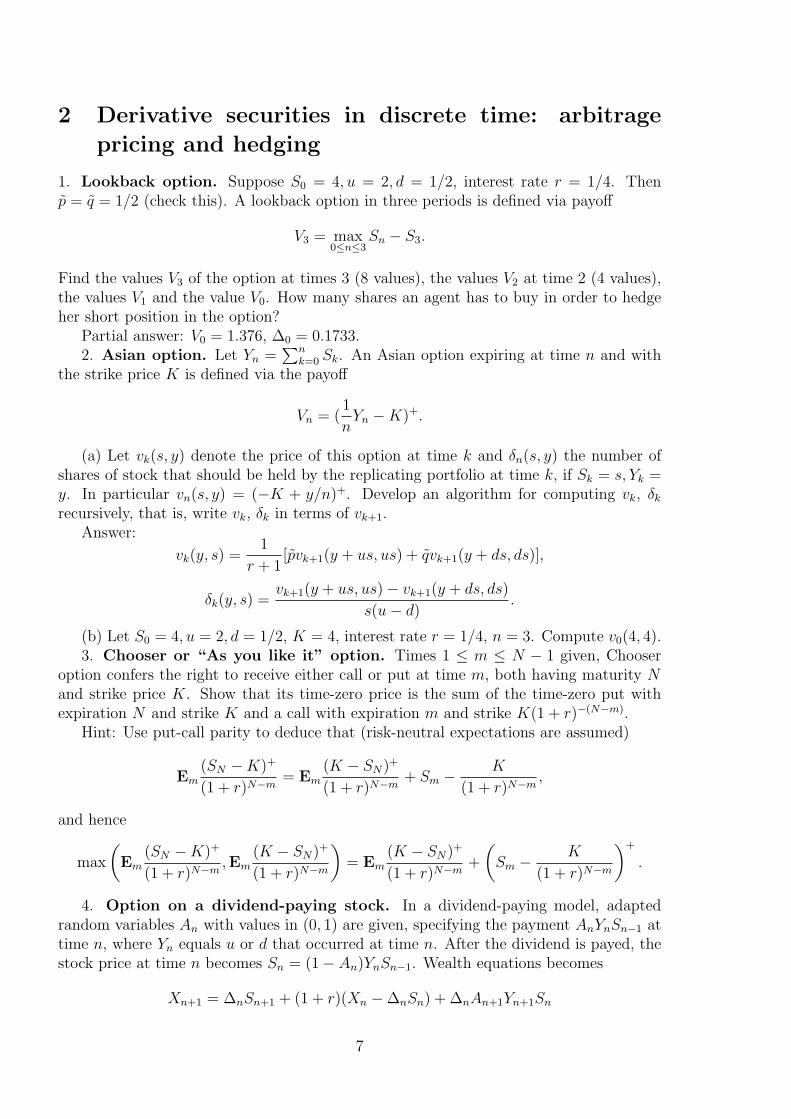
1. Lookback option. Suppose S0 = 4, u = 2, d = 1/2, interest rate r = 1/4. Thenp = q = 1/2 (check this). A lookback option in three periods is defined via payoff

V3 = max0≤n≤3

Sn − S3.

Find the values V3 of the option at times 3 (8 values), the values V2 at time 2 (4 values),the values V1 and the value V0. How many shares an agent has to buy in order to hedgeher short position in the option?

Partial answer: V0 = 1.376, ∆0 = 0.1733.2. Asian option. Let Yn =

∑nk=0 Sk. An Asian option expiring at time n and with

the strike price K is defined via the payoff

Vn = (1

nYn −K)+.

(a) Let vk(s, y) denote the price of this option at time k and δn(s, y) the number ofshares of stock that should be held by the replicating portfolio at time k, if Sk = s, Yk =y. In particular vn(s, y) = (−K + y/n)+. Develop an algorithm for computing vk, δk

recursively, that is, write vk, δk in terms of vk+1.Answer:

vk(y, s) =1

r + 1[pvk+1(y + us, us) + qvk+1(y + ds, ds)],

δk(y, s) =vk+1(y + us, us)− vk+1(y + ds, ds)

s(u− d).

(b) Let S0 = 4, u = 2, d = 1/2, K = 4, interest rate r = 1/4, n = 3. Compute v0(4, 4).3. Chooser or “As you like it” option. Times 1 ≤ m ≤ N − 1 given, Chooser

option confers the right to receive either call or put at time m, both having maturity Nand strike price K. Show that its time-zero price is the sum of the time-zero put withexpiration N and strike K and a call with expiration m and strike K(1 + r)−(N−m).

Hint: Use put-call parity to deduce that (risk-neutral expectations are assumed)

Em(SN −K)+

(1 + r)N−m= Em

(K − SN)+

(1 + r)N−m+ Sm − K

(1 + r)N−m,

and hence

max

(Em

(SN −K)+

(1 + r)N−m,Em

(K − SN)+

(1 + r)N−m

)= Em

(K − SN)+

(1 + r)N−m+

(Sm − K

(1 + r)N−m

)+

.

4. Option on a dividend-paying stock. In a dividend-paying model, adaptedrandom variables An with values in (0, 1) are given, specifying the payment AnYnSn−1 attime n, where Yn equals u or d that occurred at time n. After the dividend is payed, thestock price at time n becomes Sn = (1− An)YnSn−1. Wealth equations becomes

Xn+1 = ∆nSn+1 + (1 + r)(Xn −∆nSn) + ∆nAn+1Yn+1Sn

7

= ∆nYn+1Sn + (1 + r)(Xn −∆nSn).

Show that the discounted wealth process is a martingale under the risk-neutral measure(which are the same as in the model without dividends), that is

EmXn

(1 + r)n=

Xm

(1 + r)m, n ≥ m,

implying that the risk-neutral pricing formula

Vn = EnVN

(1 + r)N−n

for option pricing still applies. Show that if An = a is a constant, then

Sn

(1− a)n(1 + r)n

is also a martingale.Hint: It is sufficient to show the first formula for n = m + 1. Then

EmXm+1

(1 + r)m+1=

∆mSm

(1 + r)m+1EYm+1 +

Xm −∆mSm

(1 + r)m

=∆mSm

(1 + r)m+

Xm −∆mSm

(1 + r)m=

Xm

(1 + r)m.

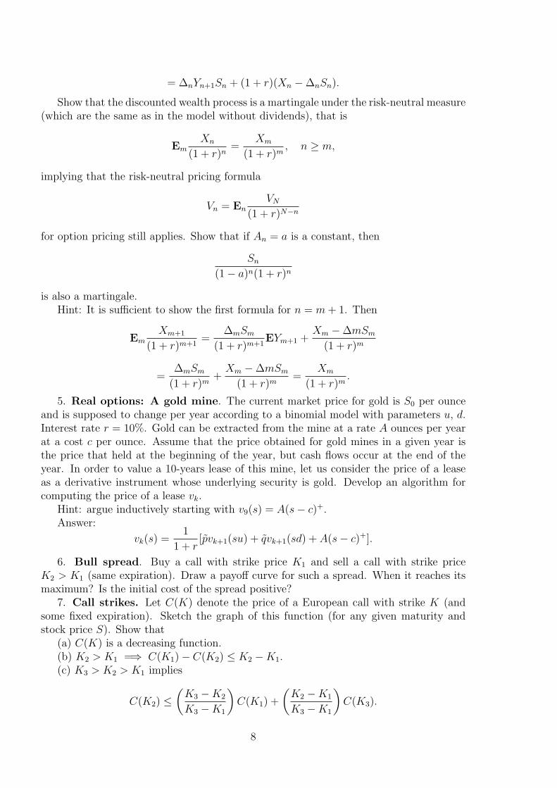
5. Real options: A gold mine. The current market price for gold is S0 per ounceand is supposed to change per year according to a binomial model with parameters u, d.Interest rate r = 10%. Gold can be extracted from the mine at a rate A ounces per yearat a cost c per ounce. Assume that the price obtained for gold mines in a given year isthe price that held at the beginning of the year, but cash flows occur at the end of theyear. In order to value a 10-years lease of this mine, let us consider the price of a leaseas a derivative instrument whose underlying security is gold. Develop an algorithm forcomputing the price of a lease vk.

Hint: argue inductively starting with v9(s) = A(s− c)+.Answer:

vk(s) =1

1 + r[pvk+1(su) + qvk+1(sd) + A(s− c)+].

6. Bull spread. Buy a call with strike price K1 and sell a call with strike priceK2 > K1 (same expiration). Draw a payoff curve for such a spread. When it reaches itsmaximum? Is the initial cost of the spread positive?

7. Call strikes. Let C(K) denote the price of a European call with strike K (andsome fixed expiration). Sketch the graph of this function (for any given maturity andstock price S). Show that

(a) C(K) is a decreasing function.(b) K2 > K1 =⇒ C(K1)− C(K2) ≤ K2 −K1.(c) K3 > K2 > K1 implies

C(K2) ≤(

K3 −K2

K3 −K1

)C(K1) +

(K2 −K1

K3 −K1

)C(K3).

8

Hint: By risk neutral pricing one should only prove it at the time of expiration. Thus (b)follows from

(S −K1)+ − (S −K2)

+ ≤ K2 −K1, K2 > K1.

Why is it true? Statement (c) follows from the convexity of the function C(K).8. One period ∆. Let ∆ denote the amount of shares needed to hedge a position of

an agent that is selling a standard European put, in a one period binomial model withstrike price K. Sketch the graph of ∆ against the initial value of stock S. Describe thedomains where this function is linear, concave or convex.

9. Setting binomial models and deflator calculations. We are interested inpricing a derivative security, written on a stock with volatility σ = 0.2 p.a., that maturesin one year. Continuously compounded risk-free rate is 4% p.a.

(a) Set up a four period binomial model and compute the risk-neutral probabilities.(b) Suppose additionally that the expected return on the stock is 2% per month.

Calculate the real world probabilities and the state price deflators (or density).(c) Price a European powered call option with expiry one year and strike K, specified

by the payoff V (S) = ((S −K)+)p. Construct a hedge portfolio.Hint: (a)

∆t = 1/4, 1 + r = e0.04/4 = e0.01, u = e0.2/√

4 = e0.1, d = e−0.1.

p = (e0.01 − e−0.1)/(e0.1 − e−0.1).

(b) Since E(S1/S0) = (1.02)3 = pu + (1− p)d (where p is real world prob.), it follows

p =(1.02)3 − d

u− d.

Deflator is a random variable taking value

e−0.04

(p

p

)l (1− p

1− p

)4−l

on the event when l among 4 moves of the stock were upwards.10. Backward calculations for European and American derivatives. Let a

current stock price is $62 and the stock volatility is σ = 0.20 Interest rates are 10%compounded monthly. Using binomial approach with period length 1 month, determinethe price of a European call and American put, both with expiration 5 months and strike$60. Display the prices of stocks and options for all months in tables. On the table forAmerican put stress the values, where the earlier exercise is optimal. Write down therecurrent equation for determining American put vn(s) (at time n, when the stock priceis S).

Partial answer: Table of stock prices:

62.00 65.68 69.59 73.72 78.11 82.7558.52 62.00 65.68 69.59 73.72

55.24 58.52 62.00 65.6852.14 55.24 58.52

49.21 52.1446.45

9

Table of the American put prices:

1.56 0.61 0.12 0 0 02.79 1.23 0.28 0 0

4.80 2.45 0.65 07.86 4.76 1.48

10.79 7.8613.55

11. Multi-factor model. Assume there are two risky assets. In one period, theinitial values (S1

0 , S20) can move to (u1S

10 , u2S

20) with probability puu, to (u1S

10 , d2S

20) with

probability pud, to (d1S10 , u2S

20) with probability pdu, or to (d1S

10 , d2S

20) with probability

pdd. Write down the equations for (risk neutral) probabilities puu, pud, pdu, pdd that ensurethat the discounted stock price processes S1

m/(1 + r)m, S2m/(1 + r)m are martingales? Is

there a unique solution for these equations?Answer:

(puu + pud)u1 + (pdu + pdd)d1 = 1 + r,

(puu + pdu)u2 + (pud + pdd)d2 = 1 + r,

puu + pud + pdu + pdd = 1.

Not unique.Recommended reading.S. E. Shreve. Stochastic Calculus for Finance I. The Binomial Asset Pricing Model.

Springer Finance. Springer, 2005.N. H. Bingham, R. Kiesel. Risk-neutral valuation. Pricing and hedging of financial

derivatives. 2nd Ed. Springer Finance. Springer, 2004.M. Baxter, A. Rennie. Financial Calculus. Cambridge University Press, 1998.A. Etheridge. A Course in Financial Calculus. Cambridge University Press, 2002.D.G. Luenberger. Investment Science. Oxford University Press, 1998.

10

3 Stochastic calculus and derivatives in continuous

time

W denotes the standard Wiener process or Brownian motion, and Φ the distributionfunction of standard normal r.v.

1. Simplest product rule. Let dX(t) = α(t)dt + β(t)dW (t) and dY (t) = ω(t)dt,where α(t), β(t), ω(t) are adapted continuous processes. Show that

d(Y (t)X(t)) = X(t)dY (t) + Y (t)dX(t) = ω(t)X(t)dt + Y (t)dX(t), (3)

ord(Y (t)X(t)) = [ω(t)X(t) + Y (t)α(t)]dt + Y (t)β(t)dW (t).

2. Vasicek interest rate model. This is given by the equation

dR(t) = (α− βR(t)) dt + σ dW (t), (4)

where α, β, σ > 0.(a) Recall (and check!) that the solution to the ODE

x = −βx + g(t), x(0) = x0,

is given by the formula (Duhamel principle)

x = e−βtx0 +

∫ t

0

e−β(t−s)g(s) ds.

Applying this result formally to the Vasicek equation, deduce its solution:

R(t) = e−βtR(0) +α

β(1− e−βt) + σe−βt

∫ t

0

eβs dW (s). (5)

(b) Check that (5) solves (19) applying Ito’s formula to the function

f(t, x) = e−βtR(0) +α

β(1− e−βt) + σe−βtx

and X(t) =∫ t

0eβs dW (s), or, alternatively, applying the Ito’s product rule (stochastic

integration by parts).(c) Find the variance of R(t).Answer: σ2(1− e−2βt)/2β.(d) Find the expectation of R(t) and show that it converges to a constant, α/β (mean-

reverting property).(e) Hull-White model. Suppose α, β, σ in (19) are not constants, but rather con-

tinuous deterministic functions of time. Deduce the corresponding generalization of thesolution formula (5).

3. Cox-Ingersoll-Ross (CIR) interest rate model. This is given by

dR(t) = (α− βR(t)) dt + σ√

R(t) dW (t), (6)

where α, β, σ > 0.

11

(a) Using (3), show that X(t) = eβtR(t) satisfies the equation

dX(t) = αeβt dt + σeβt/2√

X(t) dW (t). (7)

Use this formula to show that the expectation of R(t) coincides with the expectation ofthe Vasicek model.

(b) From the product rule deduce that

d(X2(t)) = (2α + σ2)eβtX(t) dt + 2σeβt/2X3/2(t) dW (t). (8)

Then calculate E(R2(t)) and Var (R(t)).Partial answer: Var R(t) equals

σ2

βR(0)(e−βt − e−2βt) +

ασ2

2β2(1− 2e−βt + e−2βt).

4. CIR and OU processes. Let W1, ...,Wd be independent standard BM and Xj bethe Ornstein-Uhlenbeck processes (OU) solving the equations

dXj(t)) = − b

2Xj(t)dt +

1

2σdWj(t), (9)

j = 1, ..., d.(a) Show that the process

R(t) =d∑

j=1

X2j (t)

solves the CIR equation (6) with α = dσ2/4, where

W (t) =d∑

j=1

∫ t

0

Xj(s)√R(s)

dWj(s)

is a BM (check it by Levy’s theorem!).(b) Noting that the equations for Xj are particular cases of the Vasicek equation (19),

deduce that Xj(t) are iid N(µ(t), v(t)) r.v. with

µ(t) = e−bt/2√

R(0)/d, v(t) =σ2

4b[1− e−bt].

(c) Recall that the Laplace transform and the MGF of a r.v. Z are defined respectivelyas the functions

LZ(u) = Ee−uZ , MZ(u) = EeuZ = LZ(−u).

Find the Laplace transform LX2j(u) of X2

j . Answer:

1√1 + 2uv(t)

exp

−uµ2(t)

1 + 2uv(t)

.

(d) Find the Laplace transform and the MGM of the solution R(t) to the CIR model.

12

5. Linear equations and generalized geometric BM. Consider the equation

dS(t) = S(t)(α(t)dt + σ(t)dW (t)). (10)

Let S(t) = S0eY (t).

(a) Show that

dY (t) = (α(t)− 1

2σ2(t))dt + σ(t)dW (t),

and hence deduce the formula for the solution of (10).(b) Deduce the SDE for the discounted stock price D(t)S(t), where D(t) = exp− ∫ t

0R(s)ds

and R(t) denotes the interest rate.(c) Show, in particular, that if α, σ,R are constants, then log(S(T )/S0) is normal

N((α− σ2/2)t, σ2t) and log(D(T )S(T )/S0) is normal N((α−R− σ2/2)t, σ2t).(d) Assuming α, σ,R to be constants, write down the expression for S(t) in terms of

the BM W (t) = θt+W (t), where Θ = (α−R)/σ is the market price of risk. Conclude thatunder W , log(S(T )/S0) is normal N((R − σ2/2)t, σ2t) and log(D(T )S(T )/S0) is normalN(−tσ2/2, tσ2).

Answer:S(t) = S0 expσW (t) + t(R− σ2/2).

6. Moving normal means by a change of measure. Let X be N(0, 1) r.v. definedon a probability space with the law P. Let θ > 0,

Z = exp−θX − 1

2θ2,

and probability P is defined via EY = E(ZY ), or equivalently

P(A) =

∫

A

Z(ω)dP(ω). (11)

Show that X is N(−θ, 1) under P. Hint:

EX =1√2π

∫xe−θx−θ2/2e−x2/2 dx.

7. Change of measure under filtration. Let (Ω,F ,Ft,P) be a filtered probabilityspace, t ∈ [0, T ], and Z an a.s. positive r.v. satisfying EZ = 1.

(a) Show that the Radon-Nikodym derivative process Zt = E(Z|Ft) is a martingale.(b) Let P be defined via (11). Show that

EY = E(Y Zt) (12)

for any (integrable) Ft-measurable r.v. Y , t ∈ [0, T ].(c) Let s ≤ t ≤ T and Y be again an Ft-measurable r.v. Show that

E(Y |Fs) =1

Zs

E(Y Zt|Fs). (13)

Hint: Observe that (13) is equivalent to having

E[ξ1

Zs

E(Y Zt|Fs)] = E[ξY ]

13

for any Fs-measurable ξ and use (12) to prove it.8. Calculating BS from risk-neutral evaluation formula.(a) Suppose X is log-normal, so that X = eY with a normal N(µ, σ2) r.v. Y , and let

K be a positive constant. Show that

Emax(X −K, 0) = µΦ

(ln(µ/K) + σ2/2

σ

)−KΦ

(ln(µ/K)− σ2/2

σ

), (14)

whereµ = E(X) = expµ + σ2/2.

Hint: Firstly

Emax(X −K, 0) = Emax(expµ + σZ −K, 0)

with a standard N(0, 1) r.v. Z. Consequently

Emax(X −K, 0) =

∫ ∞

(log K−µ)/σ

(eµ+σx −K)1√2π

exp

−x2

2

dx

= µ

∫ ∞

(ln K−µ)/σ

1√2π

exp

−(x− σ)2

2

dx−K

∫ ∞

(ln K−µ)/σ

1√2π

exp

−x2

2

dx,

which rewrites as (14).(b) The risk-neutral evaluation principle yields the value

c(t, x) = e−r(T−t)E[max(ST−K, 0)|S(t) = x] = xe−r(T−t)E

[max

(ST

x− K

x, 0

)|S(t) = x

],

for the price of a standard European option with maturity T and strike price K, where Emeans the expectation with respect to the risk-neutral distribution, which is log-normalwith E(ST ) = er(T−t)x, that is with log(S(T )/x)) being N((r − σ2/2)(T − t), σ2(T − t)).Prove the BS formula

c(t, x) = xΦ(d1(T − t, x))−Ke−r(T−t)Φ(d2(T − t, x))], (15)

where

d1(s, x) =log(x/K) + (r + σ2/2)s

σ√

s,

d2(s, x) =log(x/K) + (r − σ2/2)s

σ√

s.

Hint: Use (a) with µ = er(T−t) and σ√

s instead of σ.9. Basic Greeks and PDE for BS. Assume (15).(a) Find the delta of the option ∂c

∂x. Answer: Φ(d1).

(b) Find the theta of the option ∂c∂t

. Answer:

−rKe−r(T−t)Φ(d2)− σx

2√

T − tΦ′(d1).

14

(c) Find the gamma of the option ∂2c∂x2 . Answer:

1

σx√

T − tΦ′(d1(T − t, x)).

(d) Use the above formulas for Greeks to check that the function (15) satisfies the BSequation

∂c

∂t+ rx

∂c

∂x+

1

2σ2x2 ∂2c

∂x2= rc, 0 ≤ t < T, x > 0. (16)

(e) Show that

limt→T

d1,2 =

+∞, x > K,

−∞, x < K,

0, x = K

and hence the terminal condition

limt→T

c(t, x) = (x−K)+, x > 0.

(f) Show thatlimx→0

d1,2 = −∞,

and hence the boundary condition

limx→0

c(t, x) = 0.

(g) Show thatlim

x→∞d1,2 = ∞.

Use this fact to deduce the boundary condition

limx→∞

[c(t, x)− (x− e−r(T−t)K)] = 0, 0 ≤ t < T.

10. Dividends. Evolution of a stock price with a continuous dividend paying is givenby

dS(t) = S(t)[α(t)dt + σ(t)dW (t)− A(t)dt], (17)

where α(t), σ(t), A(t) are given continuous adapted processes, and of the portfolio value

dX(t) = ∆(t)dS(t) + ∆(t)A(t)S(t)dt + R(t)[X(t)−∆(t)S(t)]dt,

where R(t) and ∆(t) are adapted processes denoting respectively the (given) interest rateand the number of shares held at time t.

(a) Show that

dX(t) = R(t)X(t)dt + ∆(t)σ(t)S(t)[Θ(t)dt + dW (t)],

where Θ(t) = (α(t)−R(t))/σ(t) denotes the market price of risk.(b) Introducing the new BM via

W (t) = W (t) +

∫ t

0

Θ(u)du,

15

derive for the discount portfolio the equation

d[D(t)X(t)] = ∆(t)D(t)S(t)σ(t)dW (t),

where D(t) = exp− ∫ t

0R(u) du is the discount process.

(c) Deduce the risk-neutral pricing formula for a derivative security based on S.11. An example of a call. Suppose an option pays $1 at time T , if the share price

S(T ) lies in the interval [a, b] and nothing otherwise. Find its price at time zero.Hint:

c = e−rT E1S(T )∈[a,b]

where log(S(T )/S0)) is N((r − σ2/2)(T − t), σ2(T − t)). Hence

c = e−rT

(Φ

[log(a/S0)− (r − σ2/2)T√

Tσ

]− Φ

[log(b/S0)− (r − σ2/2)T√

Tσ

]).

12. Comparing Greeks. (a) A portfolio consists of 1 thousand shares of a stock anda number, n, of European put options, P, on this stock. The delta and the gamma of theput are -0.2 and 0.4 respectively. Find n, if the delta of the whole portfolio is zero.

Hint: (a) −0.2n + 1000 = 0, so n = 5000.(b) Two other derivatives are available on the market: a European call, C, with the

same maturity and strike as P, and a security D, with a delta of 0.2 and gamma of 0.2.Calculate the number c of derivatives C and the number d of D that have to be purchasedand added to the portfolio so that the delta and gamma of the expanded portfolio vanish.

Hint: Use the put-call parity to deduce ∆(C) = ∆(P ) + 1 and Γ(C) = Γ(P ). Next,the Gamma of the original portfolio is 0.4× 5000 = 2000. Hence we need

c(1− 0.2) + 0.2d = 0, 5000× 0.4 + 0.4c + 0.2d = 0.

13. Greeks and implied volatility calculations. A stock is priced at $8.20. Awriter of 100 units of a one year European call with an exercise price of $8 has hedgedthe option with a portfolio of 75 shares and a loan. The annual risk-free interest rate is7%.

(a) Find the Delta of the option.(b) Calculate the implied volatility of the stock to within 0.1% p.a., assuming that it

is below 100%.(c) Find the value of the loan and the price of the option contract.Hints: (a) 100∆ = 75, so that ∆ = 0.75.(b) It is known that ∆ = Φ(d1). Hence d1 = 0.6745. It follows that

0.02469 + 0.07 + 0.5σ2 = 0.6745σ.

Solving the equation (choosing the root less than one): σ = 0.159 = 15.9%.(c) The loan is 100Ke−rT Φ(d2) = 519.7 and the option contract 100 × 8.2 × 0.75 −

519.7 = 95.2.14. Term-structure equation for bond prices (and interest rates). If interests

rate evolve according to an SDE of form

dR(t) = β(t, R(t))dt + γ(t, R(t))dW , (18)

16

where W is BM under a risk-neutral measure, the discount process is D(t) = exp− ∫ t

0R(s)ds

and the zero-coupon bond pricing formula is

B(t, T ) = E(e−

∫ t0 R(s)ds|Ft

).

Since R(t) is Markov, B(t, T ) = f(t, R(t)) for some function f(t, r). Find the PDE (calledterm-structure equation) for f and state the terminal condition for t = T .

Hint 1: D(t)B(t, T ) = D(t)f(t, R(t)) should be a martingale. Hence the dt term of itsdifferential should vanish. Terminal condition f(T, r) = 1 for all r.

Hint 2:

d(D(t)f(t, R(t)) = D(t)[−Rf +∂f

∂t+ β

∂f

∂r

1

2γ2 +

∂2f

∂r2] + D(t)γ

∂f

∂rdW .

15. Bond prices under the Hull-White interest rate model. In the Hull-Whitemodel equation (18) is of the form

dR(t) = (a(t)− b(t)R(t)) dt + σ(t) dW (t), (19)

where α, β, σ are positive (deterministic) functions. The equation for f(t, r) describingthe bond price via B(t, T ) = f(t, R(t)), see previous Exer., takes the form

∂f

∂t+ (a(t)− b(t)r)

∂f

∂r+

1

2σ2(t)

∂2f

∂r2= rf.

Find the functions C(t, T ) and A(t, T ) such that this equation is satisfied by f of the form

f(t, r) = e−rC(t,T )−A(t,T ).

Show that adding the terminal condition f(T, r) = 1 for all r specify these C and Auniquely.

Partial answer: C(T, T ) = A(T, T ) = 0 and

C(t, T ) = b(t)C(t, T )− 1,

A(t, T ) = −a(t)C(t, T ) +1

2σ2(t)C2(t, T ).

16. Equivalent constant rate of interest.(a) Show, by the arbitrage argument, that if R = R(t, T1, T2) is the equivalent constant

rate of interest over the period [T1, T2] (pay 1 at time T1 and receive eR(T2−T1) at T2), asseen from time t ≤ T1, then

eR(T2−T1) =B(t, T1)

B(t, T2),

where B(t, T ) denotes the zero-coupon bond with maturity T (or T -bond), or equivalently

R = R(t, T1, T2) = − log B(t, T2)− log B(t, T1)

T2 − T1

.

Hint: Sell T1 bond and buy B(t,T1)B(t,T2)

of T2 bonds – investment zero. Then you will pay

1 at T1 and receive B(t,T1)B(t,T2)

at T2.

17

17. Interest rate evolutions (various representations). Define: the instanta-neous forward rate with maturity T , at time t

f(t, T ) = −∂ log B(t, T )

∂T, (20)

or equivalently

B(t, T ) = exp−∫ T

t

f(t, s) ds (21)

and the instantaneous short rate r(t) = f(t, t) at time t.Define Short-rate Dynamics:

dr(t) = a(t) dt + b(t) dW (t), (22)

Bond-price Dynamics

dB(t, T ) = B(t, T )[m(t, T ) dt + v(t, T ) dW (t)], (23)

Forward-rate Dynamics

df(t, T ) = α(t, T ) dt + σ(t, T ) dW (t) (24)

(starting analysis from an exogenously given SDE for forward rates is often referred to asHeath-Jarrow-Morton methodology).

Show: (i) If B(t, T ) satisfies (23), then f satisfies (24) with

α(t, T ) =∂v

∂T(t, T )v(t, T )− ∂m

∂T(t, T ), σ(t, T ) = − ∂v

∂T(t, T )

(hint: use the Ito formula);(ii) If f(t, T ) satisfies (24), then short-rate satisfies (22) with

a(t) =∂f

∂T(t, t) + α(t, t), b(t) = σ(t, t); (25)

and B(t, T ) satisfies (23) with

m(t, T ) = r(t) + A(t, T ) +1

2‖S(t, T )‖2, v(t, T ) = −S(t, T ), (26)

where

A(t, T ) = −∫ T

t

α(t, s) ds, S(t, T ) = −∫ T

t

σ(t, s) ds.

Solution: By (24),

f(t, t) = r(t) = f(0, t) =

∫ t

0

α(s, t) ds +

∫ t

0

σ(s, t) dW (s), (27)

∂f

∂T(t, t) =

∂f

∂T(0, t) =

∫ t

0

∂α

∂T(s, t) ds +

∫ t

0

∂σ

∂T(s, t) dW (s). (28)

18

Inserting there

α(s, t) = α(s, s) +

∫ t

s

∂α

∂T(s, u) du,

σ(s, t) = σ(s, s) +

∫ t

s

∂σ

∂T(s, u) du,

yields

r(t) = f(0, t) +

∫ t

0

α(s, s) ds +

∫ t

0

∫ t

s

∂α

∂T(s, u) duds

+

∫ t

0

σ(s, s) dW (s) +

∫ t

0

∫ t

s

∂σ

∂T(s, u) dudW (s),

which by changing order (stochastic Fubbini’s theorem) rewrites as

r(t) = f(0, t) +

∫ t

0

α(s, s) ds +

∫ t

0

(∫ u

0

∂α

∂T(s, u) ds

)du

+

∫ t

0

σ(s, s) dW (s) +

∫ t

0

(∫ u

0

∂σ

∂T(s, u) dW (s)

)du,

yielding (25).Turning to the second part. By (21) and Ito’s formula, to prove (26) it is sufficient to

show that Z(t) = − ∫ T

tf(t, s) ds satisfies the equation

dZ(t, T ) = (r(t) + A(t, T ))dt + S(t, T )dW (t). (29)

But from (24),

Z(t, T ) = −∫ T

t

f(0, s)ds−∫ t

0

∫ T

t

α(u, s)dsdu−∫ t

0

∫ T

t

σ(u, s)dsdW (u).

Splitting and changing the order yields

Z(t, T ) = Z(0, T ) +

∫ t

0

r(s)ds−∫ t

0

(∫ T

u

α(u, s)ds

)du−

∫ t

0

(∫ T

u

σ(u, s)ds

)dW (u),

implying (29).18. SDEs: uniqueness in law and path-wise. Show that the SDE (B is a standard

BM)dXt = sgn(Xt)dBt

(a) enjoys uniqueness in law, (b) but not a path-wise uniqueness.Hint: (a) Use the Levy theorem to show that any solution is a BM. (b) Show that, for

a given B, if X is a solution then so is −X.19. Integral representation for functionals of BM Bt. Let T > 0 is given and

f ∈ C(Rd). Define the martingale Mt = E(f(BT )|Ft). Show that it has a representation

Mt = E(f(BT )) +

∫ t

0

ωs(Bs)dBs,

19

where

ωt(x) =

∫∂

∂xpt(x− y)f(y) dy,

with pt being the heat kernel

pt(x) = (2πt)−d/2 exp−x2

2t.

Hint. By the Markov property, Mt = φt(Bt), where φ(t, x) = E(f(BT )|Bt = x). Inparticular, M0 = φ0(0). The function

φt(x) =

∫pT−t(x− y)f(y)dy

satisfies the (inverse time) heat equation. Hence it follows from Ito’s formula that

Mt = φ0(0) +

∫ t

0

∂

∂xφs(Bs) dBs.

Integration by parts yields ∂∂x

φt(x) = ωt(x).20. Credit risk: setting up a Markov chain model. (a) Suppose τ is a positive

r.v. with a differentiable distribution function. Show that there exists a non-negativecontinuous function λ(t) s.t.

P(τ > t|τ > s) = e−∫ t

s λ(u) du, s ≤ t.

When τ denotes a default time, λ(u) is called default intensity or hazard rate.Hint: Write down

P(τ > t|τ > s) = P(τ > t)/P(τ > s),

take logarithms and denote λ(u) = − ddt

log P(τ > t).(b) For a τ as above let us define a Markov chain Xt on the space of two points D,N

(default, no default) in such a way that D is an absorbing state and if Xt = N , then itstays there a random time τt: s.t. P(τt > s) = P(τ > t|τ > s) and then jumps to D.Show that this Markov chain has the following transitions:

ps,t(D,D) = 1, ps,t(D,N) = 0, ps,t(N,N) = e−∫ t

s λ(u) du, ps,t(N,D) = (1−e−∫ t

s λ(u) du),

and the following (time-nonhomogeneous) Q-matrix

Q(t) =

(− λ(t) λ(t)

0 0

)

so that

d

dt|t=sEf(Xt)|Xs = D) = 0,

d

dt|t=sEf(Xt)|Xs = N) = λ(s)(f(D)− f(N)),

for a function f on the state space D, N.

20

(c) Let B(t, T ) denote the price at time t of a zero-coupon bond that matures at timeT with payment πT that equals 1 or δ in cases N (no default till time T ) or D respectively.If λ(t) above are given with respect to the risk-neutral measure Q, and if at time t thereis no default, then

B(t, T ) = e−r(T−t)EQ(πT ).

Show thatB(t, T ) = e−r(T−t)

(δ + (1− δ)e−

∫ Tt λ(u) du

),

and hence deduce the formula

λT = − ∂

∂Tlog[er(T−t)B(t, T )− δ].

(d) Extend this model to the case of n states (credit ranking), where the last state,n, is absorbing (default) and other transitions are specified by certain rates λij(t) (TheJarrow-Lando-Turnbull model).

21. Credit risk: hedging.In a two state model let r be constant risk free rate (continuously compounded) and the

default intensity is a constant, λ, under a measure P . Consider a zero-coupon defaultablebond that is due to redeem at par in two years time. Suppose its price is given by

Bt =

δe−r(2−t), default occurred prior to time t

e−r(2−t)[δ + (1− δ)e−λ(2−t)] otherwise

(a) Show that P is EMM for this model.Hint: One has to show that

E(e−rtBt|Fs) = e−rsBs.

Analyze separately the cases when default occurred prior to s and otherwise. Say, in thefirst case, e−rtBt = e−rsBs = δe−2r.

(b) Suppose a derivative contract pays $100 after two years iff the bond has defaulted.Determine a constant portfolio in the defaultable bond and cash which replicates thederivative. Calculate the price of the derivative.

Hint: For portfolio of the form xBt + y we should have xδ + y = 100 and x + y = 0 atthe maturity, so that y = −x = 100/(1− δ). The fair price is the cost of this portfolio attime t:

ye−2r + xB0.

22. Credit risk: Merton’s model. A company has issued a zero-coupon bond ofnominal value $6 mln with maturity of one year. The value of the assets of the companyis $10 mln and this value is expected to grow at 10% p. a. compound with an annualvolatility of 30%. Shares are currently traded at a capitalization of $4 mln. The companyis expected to be wound up after one year when the assets will be used to pay off thebond holders with the remainder being distributed to the equity holder. Write down theequation for the risk free rate of interest r p.a. Which one of the above conditions issuperfluous?

Hint: S0 = 10, σ = 0.3, T = 1, K = 6. The value of the call is 4.Answer:

4 = 10Φ

[log(10/6) + r + (0.3)2/2

0.3

]− 8e−rΦ

[log(10/6) + r − (0.3)2/2

0.3

].

21