Problems compendium ie - Lnu.sehomepage.lnu.se/staff/ebape/courses/New international...Dr. Petre...
59
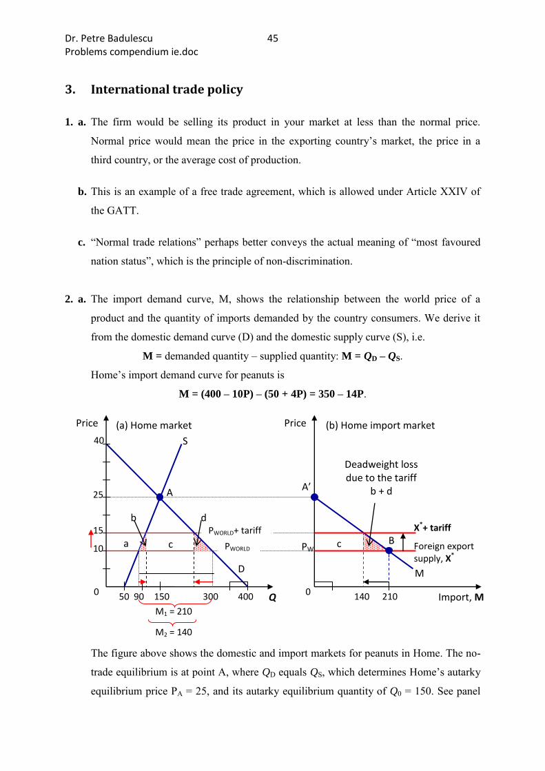
Dr. Petre Badulescu 1 Problems compendium ie.doc LINNAEUS UNIVERSITY Department of Economics and Statistics Dr. Petre Badulescu Autumn 2012 1NA400 B/International economics Problems compendium Observe! Critical comments and eventual mistakes in the text are gratefully welcomed. The Compendium contains a relatively grate number of exercises. Solutions and answers for every problem are provided at the end of the compendium. The student shall solve these problems all by oneself and check up on the own answers with the provided solutions at the end of the compendium. Notice that the provided answers are merely clues. It is always required an explanation and justification for a right answer. Furthermore graphic and mathematical descriptions shall be explained in the running text. Content Page 1. International trade theory under perfect competition 2 2. Modern international trade theory: scale economies and imperfections 13 3. International trade policy 15 Solutions 23
Transcript of Problems compendium ie - Lnu.sehomepage.lnu.se/staff/ebape/courses/New international...Dr. Petre...
Dr. Petre Badulescu 1 Problems compendium ie.doc
LINNAEUS UNIVERSITY
Department of Economics and Statistics
Dr. Petre Badulescu
Autumn 2012
1NA400 B/International economics
Problems compendium
Observe!
Critical comments and eventual mistakes in the text are gratefully welcomed.
The Compendium contains a relatively grate number of exercises. Solutions and answers
for every problem are provided at the end of the compendium. The student shall solve
these problems all by oneself and check up on the own answers with the provided
solutions at the end of the compendium. Notice that the provided answers are merely
clues. It is always required an explanation and justification for a right answer.
Furthermore graphic and mathematical descriptions shall be explained in the running
text.
Content Page
1. International trade theory under perfect competition 2
2. Modern international trade theory: scale economies and imperfections 13
3. International trade policy 15
Solutions 23

Dr. Petre Badulescu 2 Problems compendium ie.doc
1. International trade theory under perfect competition
1. Consider the graphs of the domestic markets for clothing in Sweden and Germany.
a. Is there a reason for trade in clothing between Sweden and Germany? Why?
b. Derive the appropriate export (Sx) and import (Dm) curves, assuming that”the world”
consists of only these two countries. Motivate.
c. What will happen if trade becomes possible, assuming that the cost of transportation is
negligible? What is the equilibrium trade price of clothing in Sweden? In Germany?
d. On the domestic market graphs, indicate the changes in consumer and producer
welfare which result from trade opening in each country.
e. Which groups in the two countries will be happy with free international trade in
clothing between the two countries? Which groups will wish free trade would be
banned?
f. Examine the consequences of a technology improvement which increases the
productivity in the clothing industry in Sweden. Explain!
Sweden World market Germany
c
b
Pri
ce o
f cl
oth
ing
(kilo
gram
s o
f
pap
er p
er a
rtic
le o
f cl
oth
ing)
5
4
3
2.3 2
1
SGE
DGE DSE
SSE
P
Q
P
Q
0
0
P
Q
0
a
d e

Dr. Petre Badulescu 3 Problems compendium ie.doc
2. Suppose that a small, tropical country produces mangoes for domestic consumption and
possibly for export. The domestic demand and supply curves for mangoes in this
country are given by the following expressions:
Domestic demand: P = 50 – M.
Domestic supply: P = 25 + M.
P denotes the relative price of mangoes and M denotes the quantity of mangoes (in
metric tons).
a. What are the autarky price and quantity exchanged? Motivate.
b. Suppose that the world price of mangoes is 45. Will this small country export mangoes?
If so, how many tons? Explain.
3. Home and Foreign produce and consume cars and TVs. Labor is the only input into the
production of both products. The marginal productivities of labor in each sector and the
total labor (workers) in each country are given in the following table:
Car TV Labor, L
Home 3 2 4
Foreign 2 3 4
a. What is the no-trade relative price of cars in each country? Explain.
b. In which product does Foreign have a comparative advantage, and why? Explain.
c. Graph the production possibilities frontier (PPF) for each country in separate diagrams.
Motivate briefly. d. Suppose that in the absence of trade, Home consumes nine cars and two televisions,
while Foreign consumes two cars and nine televisions. Show in your diagrams the no-
trade equilibrium for each country and provide the equilibrium conditions.
e. Suppose now that the world relative price of cars is PC/PTV = 1. In what good would
each country specialize, according to the Ricardo model? Briefly explain why?
Dr. Petre Badulescu 4 Problems compendium ie.doc
f. Show in your diagrams the international trade equilibrium for each country. Label the
exports and imports for each country at the new world price line. How does the amount
of Home exports compare with Foreign imports? Does each country gain from trade?
Briefly explain why or why not.
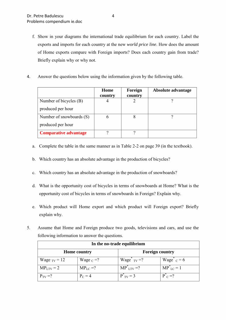
4. Answer the questions below using the information given by the following table.
Home
country
Foreign
country
Absolute advantage
Number of bicycles (B)
produced per hour
4 2 ?
Number of snowboards (S)
produced per hour
6 8 ?
Comparative advantage ? ?
a. Complete the table in the same manner as in Table 2-2 on page 39 (in the textbook).
b. Which country has an absolute advantage in the production of bicycles?
c. Which country has an absolute advantage in the production of snowboards?
d. What is the opportunity cost of bicycles in terms of snowboards at Home? What is the
opportunity cost of bicycles in terms of snowboards in Foreign? Explain why.
e. Which product will Home export and which product will Foreign export? Briefly
explain why.
5. Assume that Home and Foreign produce two goods, televisions and cars, and use the
following information to answer the questions.
In the no-trade equilibrium
Home country Foreign country
Wage TV = 12 Wage C =? Wage* TV =? Wage* C = 6
MPLTV = 2 MPLC =? MP*LTV =? MP*
LC = 1
PTV =? PC = 4 P*TV = 3 P*
C =?
Dr. Petre Badulescu 5 Problems compendium ie.doc
a. What is the marginal product of labor for televisions and cars in the Home country?
What is the no-trade relative price of televisions at Home?
b. What is the marginal product of labor for televisions and cars in Foreign? What is the
no-trade relative price of televisions at Home?
c. Suppose the world relative price of televisions in the trade equilibrium is PTV/PC = 1.
Which good will each country export? Briefly explain why.
d. In the trade equilibrium, what is the real wage at Home in terms of cars and in terms of
televisions? How do these values compare with the real wage in terms of either good in
the no-trade equilibrium? Briefly explain why.
e. In the trade equilibrium, what is the real wage in Foreign in terms of televisions and in
terms of cars? How do these values compare with the real wage in terms of either good
in the no-trade equilibrium? Briefly explain why.
f. In the trade equilibrium, do Foreign workers earn more or less than those at Home,
measured in terms of their ability to purchase goods? Explain why.
6. Suppose that the technology for creating manufacturing goods is
MM LKQ , where
QM is manufacturing output, K is the country’s endowment of capital, the factor
specific to manufacturing, and LM is the amount of the mobile factor, labor, used in
manufacturing industry.
a. How much does QM rise if both inputs ),( MLK are doubled? b. Now suppose that K is fixed at 100. How much does QM rise if LM is doubled? c. Is the cost of lost manufacturing output associated with reducing manufacturing
employment by one employee larger or smaller when the initial level of employment is
100 or 10? Motivate.

Dr. Petre Badulescu 6 Problems compendium ie.doc
7. Suppose that there are two products: Agriculture (A) and Manufacturing (M) in an
economy. Agriculture is produced with Land and Labor and Manufacturing is produced
with Capital and Labour. Labour is mobile between industries. The next two questions
refer to the production possibilities frontier (PPF) in Figure 1 below.
a. Is the opportunity cost of M higher at point 1 or point 2 in Figure 1? Motivate.
b. Provide an intuitive explanation for why the PPF is “bowed out” in Figure 1.
c. If the price of a manufactured product is PM = $10/unit and the marginal product of
labour in manufacturing is 2 units per worker, what must the wage paid to a unit of
labour be? Briefly explain.
d. If PM > PA, in which industry is the marginal product of labour higher? e. Assume that you own a manufacturing firm. If PM = $10/unit, the wage is $25, and the
marginal product of labour is 4 units per worker, are you hiring too many, too few, or
the right amount of labour. Explain.
f. Suppose the price of manufactured products in terms of agricultural products falls.
What would you expect to happen to the marginal product of labour in agriculture?
Explain.
2
1
Figure 1: PPF
0 M
A
Dr. Petre Badulescu 7 Problems compendium ie.doc
8. In the gains from trade diagram (Figure 3-3, page 63 in the textbook), suppose that
instead of having a rise in the relative price of manufactures, there is a fall in that
relative price.
a. Starting at the no-trade point A (Figure 3-3), show what would happen to production
and consumption. Motivate.
b. Which product is exported and which is imported? Why?
c. Explain why the overall gains from trade are still positive.
9. Use the information given here to answer the following questions. Manufacturing (M) Agriculture (A)
Sales revenue: 150MM QP 150AA QP
Payments to labour: 100MLW 50ALW
Payments to capital: 50KRM 100KRM
Holding the price of manufacturing constant, suppose the increase in the price of
agriculture is 10% and the increase in the wage is 5%.
a. Determine the impact of the increase in the price of agriculture on the rental on land and
the rental of capital. Motivate.
b. Explain what has happened to the real rental on land and the real rental on capital.
c. If the price of manufacturing were to fall by 10%, would landowners or capital owners
be better off? Explain. How would the decrease in the price of manufacturing affect
labour? Explain.

Dr. Petre Badulescu 8 Problems compendium ie.doc
10. Home and Foreign produce autos from capital and labor and bananas from land and
labour. Labour is mobile between the two industries. The no-trade equilibrium in the
two countries is illustrated in the diagrams below.
a. Explain how the price of autos relative to bananas is determined in the absence of trade.
b. In the diagrams above show candidate equilibrium if the two countries are trading with
each other. Indicate how production and consumption have changed in the two
countries.
c. How has the real rental to capital changed in Home? Explain. How has the real rental to
capital changed in Foreign? Explain.
d. What happens to the demand for land in Home? Motivate.
e. If the winners could without cost compensate the losers, would the countries engage in
free trade? Motivate.
0 0
Bananas Bananas
Autos Autos
Home Foreign
Dr. Petre Badulescu 9 Problems compendium ie.doc
11. This problem uses the Heckscher-Ohlin model to predict the direction of trade. Consider
the production of hand-made rugs and assembly line robots in Canada and India.
Assume the only two factors of production are labour and capital.
a. Which country would you expect to be relatively labour-abundant, and which capital-
abundant? Why?
b. Which industry would you expect to be relatively labour-intensive, and which is
capital-intensive? Why?
c. Given your answers to a) and b), draw production possibilities frontiers (PPF) for each
country. Assuming that consumer preferences are the same in both countries, add
indifference curves and relative price lines (without trade) to your PPF graphs. What do
the slopes of the price lines tell you about the direction of trade? Motivate.
d. Allowing for trade between countries, redraw the graphs (with post-trade equilibrium)
and include a “trade triangle” for each country. Identify and label the vertical and
horizontal sides of the triangles as either imports or exports. Which factors gain and
which factors lose when trade arises between these two countries? Explain carefully.
12. Suppose that there are drastic technological improvements in shoe production at Home
such that shoe factories can operate almost completely with computer-aided machines.
Consider the following data for the Home country:
Computers (C) Shoes (S)
Sales revenue: 100CC QP 100SS QP
Payments to labour: 50CLW 5SLW
Payments to capital: 50CKR 95SKR
Percentage increase in the price = %0/ CC PP %50/ SS PP
a. Which industry is capital-intensive? Is this a reasonable question, given that some
industries are capital-intensive in some countries and labour-intensive in others?

Dr. Petre Badulescu 10 Problems compendium ie.doc
b. Given the percentage changes in output prices in the data provided, calculate the
percentage change in the rental on capital. How does the magnitude of this change
compare with that of labour?
c. Which factor gains in real terms, and which factor loses? Are these results consistent
with the Stolper-Samuelson theorem? Explain.
13. The following are data on U.S. export and imports in 2007 at the two-digit Harmonized
Schedule (HS) level. Which products do you think support the Heckscher-Ohlin
theorem? Which products are inconsistent? Briefly explain.
(See problem 9, page 122 in the textbook!) Export Import
HS Code Product ($ billions) ($ billions) 22 Beverages 3.6 14.7 30 Pharmaceutical products 40.7 55.6 52 Cotton 4.9 0.8 61 Apparel 1.9 33.3 64 Footwear 1.0 17.6 72 Iron and steel 15.4 12.4 74 Copper 5.0 6.4 85 Electric machinery 124.9 212.1 87 Vehicles 73.6 131.9 88 Aircraft 83.0 18.4 94 Furniture 7.0 30.1 95 Toys 7.0 27.6
Source: International Trade Administration, U.S. Department of Commerce.
14. Consider a country that produces two products: airplanes and shirts. The country is
trading to the rest of the world at fixed product prices. Airplane producers are using 5
units of capital and 3 units of labour to produce one unit of airplanes and shirt
producers are using 2 units of capital and 2 units of labour to produce one shirt. Both
factors are mobile between industries.
a. Which product is capital-intensive? Motivate.
b. Suppose there is a sudden emigration (outflow of labour). What happens to the level of
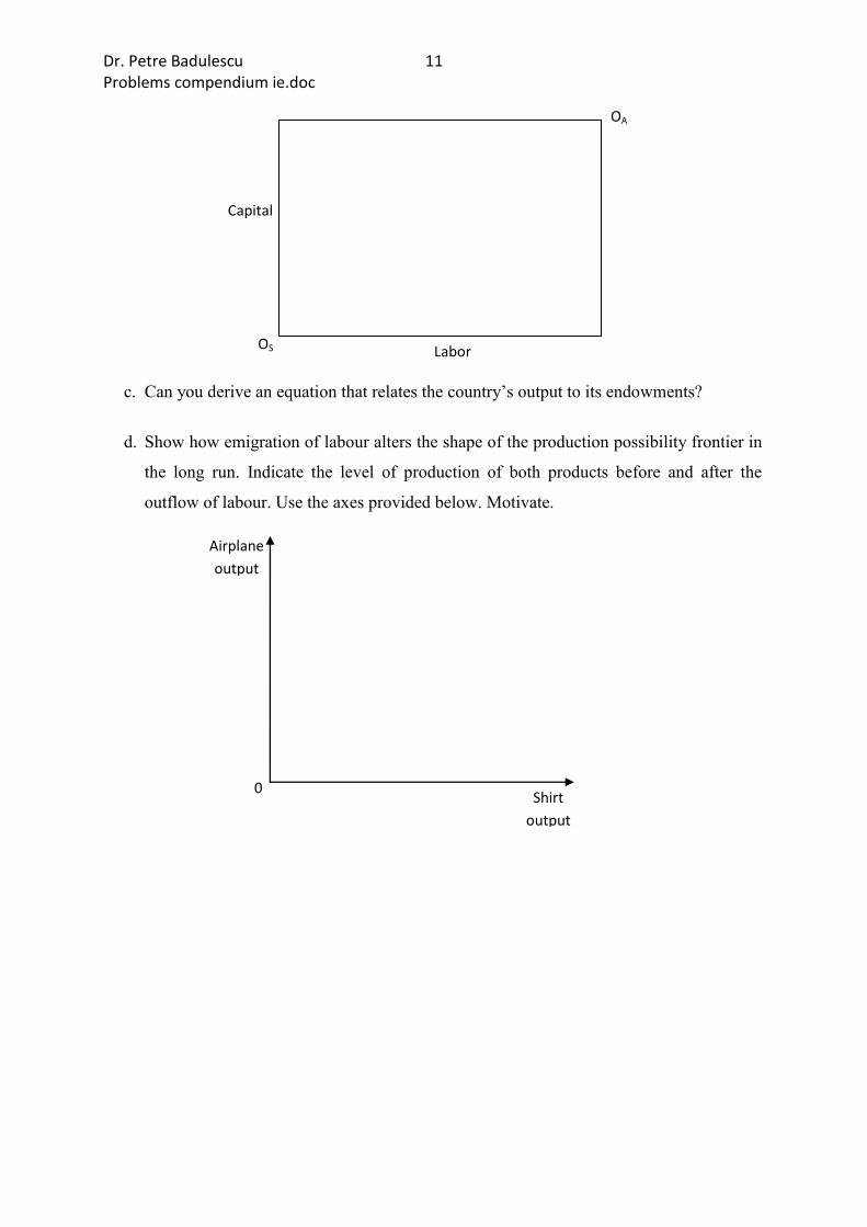
employment in the airplane industry in the long run? Show using the box diagram
provided below. Motivate.
Dr. Petre Badulescu 11 Problems compendium ie.doc
c. Can you derive an equation that relates the country’s output to its endowments?
d. Show how emigration of labour alters the shape of the production possibility frontier in
the long run. Indicate the level of production of both products before and after the
outflow of labour. Use the axes provided below. Motivate.
OA
OS Labor
Capital
0 Shirt
output
Airplane
output

Dr. Petre Badulescu 12 Problems compendium ie.doc
15. There are two countries, Home and Foreign. The two countries are identical except that
Home has a labour force of L and Foreign has a labour force of L*. The figure below is
a supply and demand for the world labour market.
Starting at points A and A*, consider a situation in which some Foreign workers migrate
to Home but not enough to reach the equilibrium with full migration (point B). As a
result of the migration, the Home wage decreases from W to W’’> W’, and the Foreign
wage increases from W* to W** < W’.
a. Are there gains that accrue to the Home country? If so, redraw the graph and identify
the magnitude of the gains for each country. If not, say why not.
b. Are there gains that accrue to the Foreign country? If so, again show the magnitude of
these gains in the diagram and also show the world gains. Motivate.
c. Suppose now that L = 100 and L*= 200. Given this allocation of labour across Home
and Foreign, the value of marginal product of labour in Home is 30 (= W) and in
Foreign 20 (= W*). If labour were to be free to move, the wage in both countries would
be 25 = W’ and L’= 150.
i.) If immigration were free between countries, how much would the value of output
change in Home? ii.) What is Home’s national gain in allowing immigration? iii.)
Who benefits from immigration in Home and how much. Briefly explain.
World amount of labour
← *L
W*
W’
W A
B
A*
L L’ 0* 0
Home
wage
Foreign
wage
Wage, W
L →

Dr. Petre Badulescu 13 Problems compendium ie.doc
2. Modern international trade theory: scale economies and
imperfections
1. Explain how increasing returns to scale in production can be a basis for trade. 2. A firm faces a fixed cost of €100 and a marginal cost of €2 per unit of output. If the
firm is planning to sell 10 units, what is the lowest price that the firm can charge that
will allow it to break even? Motivate.
3. In the following diagram, D/N is industry demand divided by the number of
differentiated products when each product has the same price and d is the demand curve
facing each individual producer of a differentiated product in an existing national
market.
a. Draw in the diagram the effect on d and D/N of an increase in N, the number of
competing varieties within the existing market.
b. Explain why you drew the demand curves as you did. 4. Starting from the long-run equilibrium in the monopolistic competition model, consider
what happens when industry demand D increases. For instance, suppose that this is the
market for cars, and lower gasoline prices generate higher demand D.
a. Draw d diagram for the Home market and show the shift in the D/NT curve and the new
short-run equilibrium.
b. From the new short-run equilibrium, is there exit or entry of firms, and why?
0 Quantity
Price
d
D/N

Dr. Petre Badulescu 14 Problems compendium ie.doc
c. Describe where the new long-run equilibrium occurs, and explain what has happened to
the number of firms and the prices they charge.
5. The Gravity equation relationship derived from the monopolistic competition model
does not hold in the Heckscher-Ohlin (H-O) model. Explain how the logic of the
gravity equation breaks down in the H-O model.
6. The United States, France and Italy are among the world’s larger producers. To answer
the following questions, assume that their markets are monopolistically competitive,
and use the gravity equation with B = 93 and n = 1.25.
GDP in 2009
($ billions)
Distance from the
United States (miles)
France 2,635 5,544
Italy 2,090 6,229
United States 14,270 –
a. Using the gravity equation compare the expected level of trade between the United
States and France and between the United States and Italy.
b. The distance between Paris and Rome is 694 miles. Would you expect more French
trade with Italy or with the United States? Explain what variable (i.e., country size or
distance) drives your result.
7. Different soil conditions generate variation in the character of grapes and the wine that
is made from them. Is it possible that intra-industry trade can be high in certain
industries even in the absence of imperfect competition? Briefly explain.
Dr. Petre Badulescu 15 Problems compendium ie.doc
3. International trade policy
1. This question tests your knowledge of the WTO’s rules. a. How would you know if a foreign firm was dumping its product in your domestic
market?
b. Assume that several countries decided to reduce tariffs exclusively on each other’s
products but maintain their tariffs on other countries’ products. Would this argument
violate the WTO’s “most favoured nation” principle? Why or why not?
c. Why is “most favoured nation status” called “normal trade relations” in the United
States? 2. Suppose that the domestic demand (D) and supply (S) for peanuts in the small country
Home are given by
D: Q = 400 – 10P and S: Q = 50 + 4P.
a. Derive the country’s import demand curve for peanuts. Draw the graphs for the
domestic and import markets. Briefly explain.
b. What are the levels of domestic production, consumption, and imports if the world
price is 10? Motivate.
c. Suppose that the country were to impose a tariff of 5. What happens to the quantity
and price of peanuts produced domestically? What happens to the quantity of
imports? Explain, calculate and illustrate these changes on your graphs.
d. What is the value of tariff revenue raised by this tariff? What is the overall gain or
loss in welfare due to the tariff introduction? Estimate and motivate.

Dr. Petre Badulescu 16 Problems compendium ie.doc
3. Consider a large country applying a tariff t to imports of a product like that represented
in the following figure.
a. How does the export supply curve in panel (b) compare with that in the small-country
case? Explain why these are different.
b. How does the import tariff t affect the free trade equilibrium? What is the net impact on
the large country welfare? Does this tariff raise or lower Foreign welfare? Explain and
illustrate the welfare impact in your graphs.
c. Explain how the tariff affects the price paid by consumers in the importing country and
the price received by producers in the exporting country. Use graphs to illustrate how
the prices are affected if (i) the export supply curve is very elastic (flat) or (ii) the
export supply curve is inelastic (steep).
4. a. The optimal tariff formula states that the tariff that raises national welfare the most is
inversely related to the elasticity of the export supply curve. Provide an intuitive
explanation for why this is so.
b. If the foreign export supply is less than perfectly elastic, what is the formula for the
optimal tariff Home should apply to increase welfare?
Price Price
S1 D1
PWORLD B*
S
QW
M
X*
Q Quantity
(b) World market (a) Importer’s domestic market
A’ A
D
0 0
Dr. Petre Badulescu 17 Problems compendium ie.doc
c. What happens to Home welfare if it applies a tariff higher than the optimal tariff?
Motivate.
5. Refer to the graphs in Problem 3. Suppose that instead of a tariff, Home applies an
import quota limiting the amount Foreign can export to 140 units.
a. Determine the net effect of the import quota on the Home economy if the quota licenses
are allocated to local producers.
b. Calculate the net effect of the import quota on the Home welfare if the quota rents are
earned by Foreign exporters.
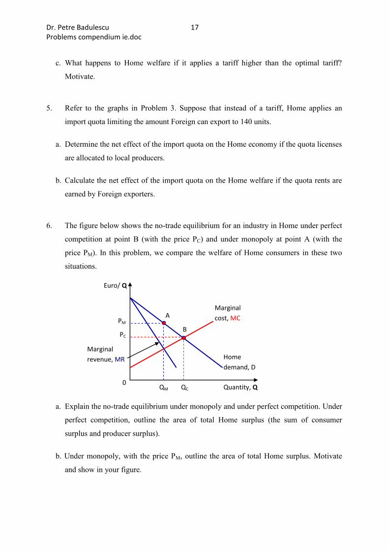
6. The figure below shows the no-trade equilibrium for an industry in Home under perfect
competition at point B (with the price PC) and under monopoly at point A (with the
price PM). In this problem, we compare the welfare of Home consumers in these two
situations.
a. Explain the no-trade equilibrium under monopoly and under perfect competition. Under
perfect competition, outline the area of total Home surplus (the sum of consumer
surplus and producer surplus).
b. Under monopoly, with the price PM, outline the area of total Home surplus. Motivate
and show in your figure.
A
B PC
PM
QC QM
Marginal
cost, MC
0
Euro/ Q
Quantity, Q
Home
demand, D
Marginal
revenue, MR
Dr. Petre Badulescu 18 Problems compendium ie.doc
c. Compare your answer to parts a) and b), and outline what the difference between these
two areas is. What is this difference called and why? Explain.
7. Suppose now that Home, from Problem 6, engages in international trade. We treat
Home as a “small country”, facing the world price of PW.
a. Explain the free-trade equilibrium under perfect competition and under monopoly. Use
a graph like the one in Problem 6 to show the Home free-trade equilibria.
b. What is the welfare impact at Home from international free trade, (i) under perfect
competition and (ii) under monopoly? Outline the area of gains or losses under (i) and
(ii) in your figure. Explain.
c. Given Home monopoly producer surplus in autarky equilibrium, and based on your
answer to part b. (ii), outline the area of gains from free trade under Home monopoly.
d. Compare your answer to parts b. (i) and c). That is, which area of gains from free trade
is higher and why? Explain.
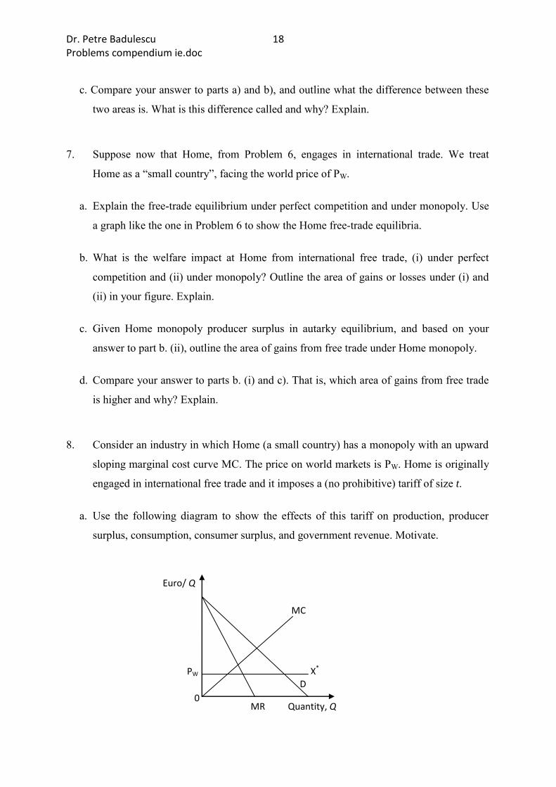
8. Consider an industry in which Home (a small country) has a monopoly with an upward
sloping marginal cost curve MC. The price on world markets is PW. Home is originally
engaged in international free trade and it imposes a (no prohibitive) tariff of size t.
a. Use the following diagram to show the effects of this tariff on production, producer
surplus, consumption, consumer surplus, and government revenue. Motivate.
X* PW D
MR
Euro/ Q
Quantity, Q 0
MC

Dr. Petre Badulescu 19 Problems compendium ie.doc
b. Now suppose instead that the government imposes a quota that yielded the same level
of imports as the tariff t. Which policy (the quota or the tariff) has a larger effect on
consumer surplus? Explain.
c. Would the quota rent created by this quota be bigger than, smaller than, or exactly the
same as the revenue generated by the tariff? Explain.
9. Consider the case of a Foreign monopoly with no Home production. For simplicity, we
assume that marginal cost are constant, MC*. Starting from free trade equilibrium,
consider a $10 tariff applied by the Home government.
a. If the demand curve is linear, what is the shape of the marginal revenue curve? Briefly
explain the free-trade equilibrium.
b. Therefore, how much does the tariff-inclusive Home price increase because of the tariff,
and how much does the net-of-tariff price received by the Foreign firm fall?
c. Discuss the welfare effects of implementing the tariff. Use a graph to illustrate under
what conditions, if any, there are increases in Home welfare.
10. Suppose that in response to a threatened antidumping duty of t, the Foreign monopoly
raises its price by the amount, t.
a. Illustrate the losses for the Home country. b. How do these losses compare with the losses from a safeguard tariff of the amount t,
applied by the Home country against the Foreign monopolist?
c. In view of your answers to (a) and (b), why are antidumping cases filed so often? 11. Why is it necessary to use a market failure to justify the use of infant industry protection?
12. What is a positive externality? Explain the argument of knowledge spillovers as a
potential reason for infant industry protection.
Dr. Petre Badulescu 20 Problems compendium ie.doc
13. If infant industry protection is justified, is it better for the Home country to use a tariff or
a quota, and why?
14. Consider a large country with export subsidies in place for agriculture. Suppose the
country changes its policy and decides to cut its subsidies in half.
a. Are there gains or losses to the large country, or is it ambiguous? What is the impact on
domestic prices for agriculture and on the world price?
b. Suppose a small food-importing country abroad responds to the lowered subsidies by
lowering its tariffs on agriculture by the same amount. Are there gains or losses to the
small country, or is it ambiguous? Explain.
c. Suppose a large food-importing country abroad reciprocates by lowering its tariffs on
agricultural goods by the same amount. Are there gains or losses to this large country,
or is it ambiguous? Explain.
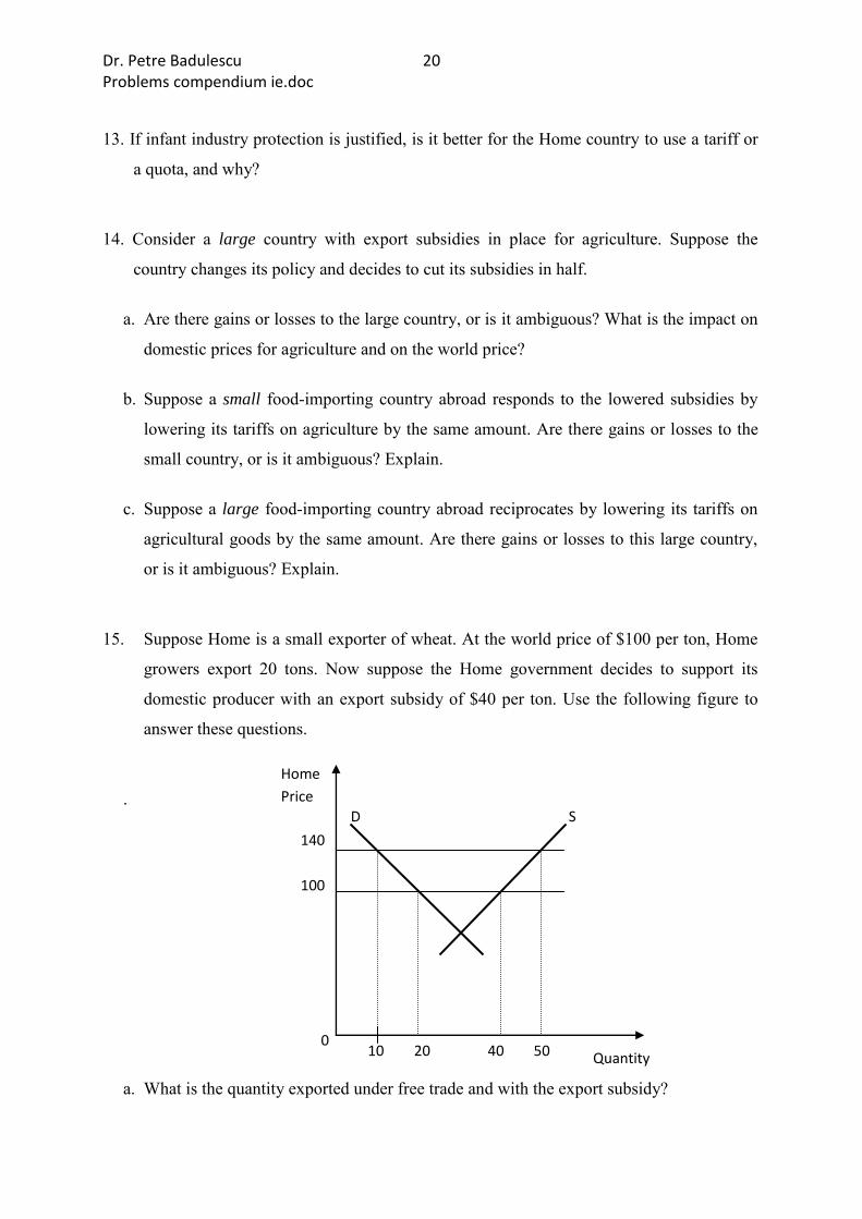
15. Suppose Home is a small exporter of wheat. At the world price of $100 per ton, Home
growers export 20 tons. Now suppose the Home government decides to support its
domestic producer with an export subsidy of $40 per ton. Use the following figure to
answer these questions.
.
a. What is the quantity exported under free trade and with the export subsidy?
140
100
Home
Price
Quantity 0
50 40 10 20
D S

Dr. Petre Badulescu 21 Problems compendium ie.doc
b. Calculate the effect of the export subsidy on consumer surplus, producer surplus, and
government revenue.
c. Calculate the overall net effect of the export subsidy on Home welfare. 16. Refer to problem 15. Rather than a small exporter of wheat, suppose that Home is a
large country. Continue to assume that the free-trade world price is $100 per ton and
that the Home government provides the domestic producer with an export subsidy in
the amount of $40 per ton. Because of the export subsidy, the local price increases to
$120 while the foreign market price declines to $80 per ton. Use the following figure to
answer the following questions.
a. Relative to the small-country case, why does the new domestic price increase by less
than the amount of the subsidy?
b. Calculate the effect of the export subsidy on consumer surplus, producer surplus, and
government revenue.
c. Calculate the overall net effect of the export subsidy on Home welfare. Is the large
country better or worse off compared with the small country with the export subsidy?
Explain.
80
120
100
Home
Price
Quantity 0
48 40 12 20
D S
Dr. Petre Badulescu 22 Problems compendium ie.doc
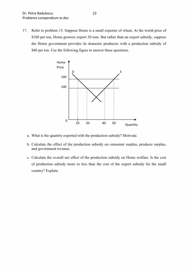
17. Refer to problem 15. Suppose Home is a small exporter of wheat. At the world price of
$100 per ton, Home growers export 20 tons. But rather than an export subsidy, suppose
the Home government provides its domestic producers with a production subsidy of
$40 per ton. Use the following figure to answer these questions.
a. What is the quantity exported with the production subsidy? Motivate. b. Calculate the effect of the production subsidy on consumer surplus, producer surplus,
and government revenue. c. Calculate the overall net effect of the production subsidy on Home welfare. Is the cost
of production subsidy more or less than the cost of the export subsidy for the small
country? Explain.
140
100
Home
Price
Quantity 0
50 40 10 20
D S
Dr. Petre Badulescu 23 Problems compendium ie.doc
Solutions
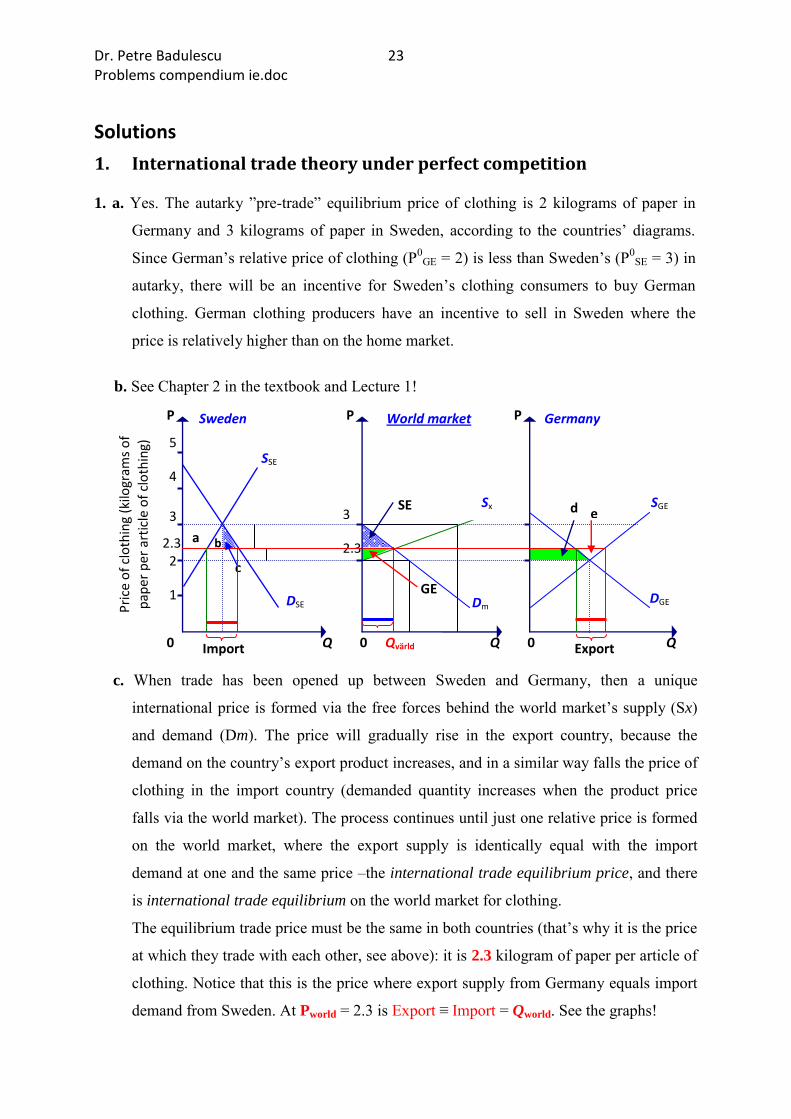
1. International trade theory under perfect competition 1. a. Yes. The autarky ”pre-trade” equilibrium price of clothing is 2 kilograms of paper in
Germany and 3 kilograms of paper in Sweden, according to the countries’ diagrams.
Since German’s relative price of clothing (P0GE = 2) is less than Sweden’s (P0
SE = 3) in
autarky, there will be an incentive for Sweden’s clothing consumers to buy German
clothing. German clothing producers have an incentive to sell in Sweden where the
price is relatively higher than on the home market.
b. See Chapter 2 in the textbook and Lecture 1!
c. When trade has been opened up between Sweden and Germany, then a unique
international price is formed via the free forces behind the world market’s supply (Sx)
and demand (Dm). The price will gradually rise in the export country, because the
demand on the country’s export product increases, and in a similar way falls the price of
clothing in the import country (demanded quantity increases when the product price
falls via the world market). The process continues until just one relative price is formed
on the world market, where the export supply is identically equal with the import
demand at one and the same price –the international trade equilibrium price, and there
is international trade equilibrium on the world market for clothing.
The equilibrium trade price must be the same in both countries (that’s why it is the price
at which they trade with each other, see above): it is 2.3 kilogram of paper per article of
clothing. Notice that this is the price where export supply from Germany equals import
demand from Sweden. At Pworld = 2.3 is Export ≡ Import = Qworld. See the graphs!
Export
DSE
SE
GE
3
2.3
2
Germany World market
c
b
Pri
ce o
f cl
oth
ing
(kilo
gram
s o
f
pap
er p
er a
rtic
le o
f cl
oth
ing)
5
4
3
2.3 2
1
SGE
DGE Dm
SSE
P
Q
P
Q
0
0
P
Q
0
a
d e Sx
Qvärld
Sweden
Import
Dr. Petre Badulescu 24 Problems compendium ie.doc
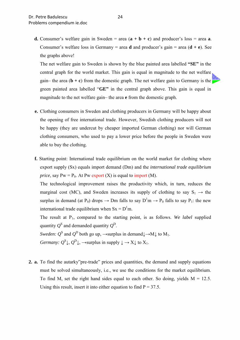
d. Consumer’s welfare gain in Sweden = area (a + b + c) and producer’s loss = area a.
Consumer’s welfare loss in Germany = area d and producer’s gain = area (d + e). See
the graphs above!
The net welfare gain to Sweden is shown by the blue painted area labelled “SE” in the
central graph for the world market. This gain is equal in magnitude to the net welfare
gain– the area (b + c) from the domestic graph. The net welfare gain to Germany is the
green painted area labelled “GE” in the central graph above. This gain is equal in
magnitude to the net welfare gain– the area e from the domestic graph.
e. Clothing consumers in Sweden and clothing producers in Germany will be happy about
the opening of free international trade. However, Swedish clothing producers will not
be happy (they are undercut by cheaper imported German clothing) nor will German
clothing consumers, who used to pay a lower price before the people in Sweden were
able to buy the clothing.
f. Starting point: International trade equilibrium on the world market for clothing where
export supply (Sx) equals import demand (Dm) and the international trade equilibrium
price, say Pw = P0. At Pw export (X) is equal to import (M).
The technological improvement raises the productivity which, in turn, reduces the
marginal cost (MC), and Sweden increases its supply of clothing to say S1 → the
surplus in demand (at P0) drops → Dm falls to say D1m → P0 falls to say P1: the new
international trade equilibrium when Sx = D1m.
The result at P1, compared to the starting point, is as follows. We label supplied
quantity QS and demanded quantity QD.
Sweden: QS and QD both go up, →surplus in demand↓→M↓ to M1.
Germany: QS↓, QD↓, →surplus in supply ↓ → X↓ to X1.
2. a. To find the autarky”pre-trade” prices and quantities, the demand and supply equations
must be solved simultaneously, i.e., we use the conditions for the market equilibrium.
To find M, set the right hand sides equal to each other. So doing, yields M = 12.5.
Using this result, insert it into either equation to find P = 37.5.
Dr. Petre Badulescu 25 Problems compendium ie.doc
b. If the world price is 45, this country would be an exporter of mangoes, because 37.5 <
45. To find out how many it would export, construct an export supply equation, that is,
an excess supply equation. Algebraically, this is done by subtracting demand from
supply (both expressed in terms of M):
Export supply Sx = Domestic supply – Domestic demand
= P – 25 – (50 – P).
Sx = –75 + 2P.
If the world price equals 45, then this country will export 15.
Observe that you could also obtain this result by substituting 45 for P in domestic
supply and demand equations to find the quantity supplied and demanded at the price
and calculating the surplus available for export.
3. a. The no-trade relative price of cars at Home is PC/PTV = 2/3, which means that to produce
one more car costs 2/3 TV. At Foreign it is P*C/P*
TV = 3/2.
b. Foreign has a comparative advantage in producing televisions because it has a lower
opportunity cost than Home in the production of televisions.
c. Home’s equation of the production possibilities frontier (PPF) is:
TV = 8 – (2/3) Cars
At Home can be maximal produced 12 cars when all resources (labour) are used in the
car industry or 8 TVs when all labour is used for the production of televisions. The
absolute value of the slope of the PPF gives the opportunity cost of cars in terms of
televisions, and equals the relative price of cars, i.e.
PC/PTV = – (MPLTV/MPLC) = – 2/3.
Foreign’s equation of the production possibilities frontier is:
Cars = 12 – (3/2) TV
In Foreign can be maximal produced 8 cars when all resources (labour) are used in the
car industry or 12 TVs when all labour is used for the production of televisions. The
absolute value of the slope of the PPF gives the opportunity cost of cars in terms of
televisions, and equals the relative price of cars, i.e.
P*C/P*
TV = – (MP*LTV/MP*
LC) = – 3/2.
Draw the diagrams here! See below 3.d!
Dr. Petre Badulescu 26 Problems compendium ie.doc
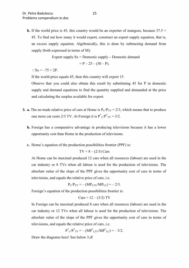
d. Add the indifference curve for each country to the diagrams in problem 3.c. Label the
indifference curve (U0), and the no-trade equilibrium production and consumption for
each country. Home no-trade consumption point is A: (cars, TVs) = (9, 2). Foreign no-
trade consumption A*: (cars, TVs) = (2, 9).
Se the diagrams!
The equilibrium conditions – the tangency point between the PPF and the U0:
consumers’ willingness to pay for a car in terms of televisions, i.e. the opportunity cost
of an extra car [measured by the absolute value of the slope of the indifference curve at
the tangency point to the PPF) must equal the opportunity cost of producing that car
(the absolute value of the slope of the PPF at the tangency point to the U0).
e. The world relative price of cars is PC/PTV = 1. The classical theory of international trade
(Ricardo) will predict that each country specializes fully (because of a constant
opportunity cost of cars-strait line PPF) in the production of the product in which it has
a comparative advantage, and export it to the other country, and import the other
product from the other country.
Home would specialize in cars, export cars, and import televisions, whereas the foreign
country would specialize in television, export televisions, and import cars. The reason is
because Home has a comparative advantage in the production of cars and Foreign in the
production of televisions.
9
12 Cars (Units)
A*
A
U*0
U0
PPF*
PPF
2 9
2
12
TV
(units)
TV*
(units)
Cars* (Units)
0 0 8
8 Slope = –2/3
Slope = –3/2
Home Foreign
Dr. Petre Badulescu 27 Problems compendium ie.doc
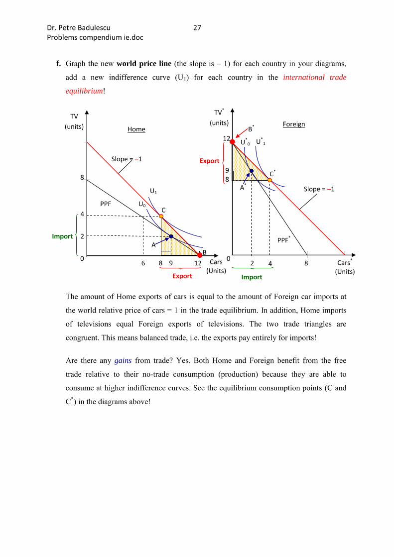
f. Graph the new world price line (the slope is – 1) for each country in your diagrams,
add a new indifference curve (U1) for each country in the international trade
equilibrium!
The amount of Home exports of cars is equal to the amount of Foreign car imports at
the world relative price of cars = 1 in the trade equilibrium. In addition, Home imports
of televisions equal Foreign exports of televisions. The two trade triangles are
congruent. This means balanced trade, i.e. the exports pay entirely for imports!
Are there any gains from trade? Yes. Both Home and Foreign benefit from the free
trade relative to their no-trade consumption (production) because they are able to
consume at higher indifference curves. See the equilibrium consumption points (C and
C*) in the diagrams above!
U*0
12
Export
Export
Import
C*
C
9 8
4
U*1
U1
6
4
12 Cars (Units)
B*
B
A*
A
U0
PPF*
PPF
2 8 9
2
TV
(units)
TV*
(units)
Cars* (Units)
0 0 8
8
Slope = –1
Slope = –1
Home Foreign
Import
Dr. Petre Badulescu 28 Problems compendium ie.doc
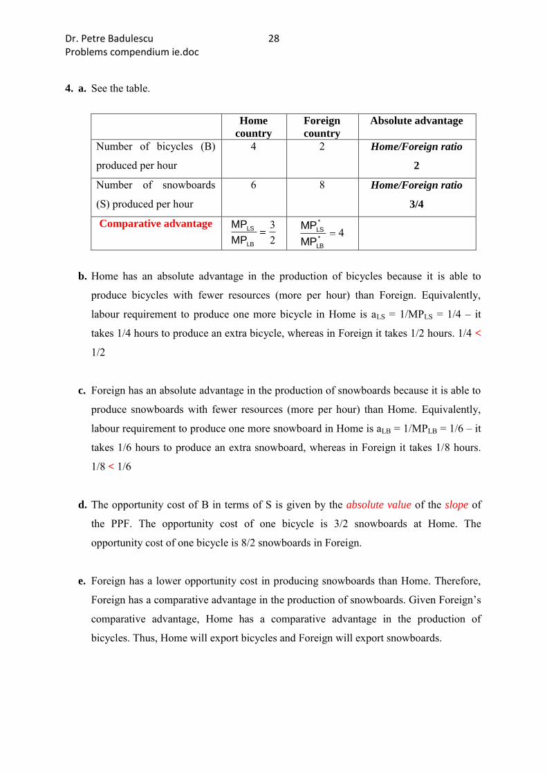
4. a. See the table.
Home
country
Foreign
country
Absolute advantage
Number of bicycles (B)
produced per hour
4 2 Home/Foreign ratio
2
Number of snowboards
(S) produced per hour
6 8 Home/Foreign ratio
3/4
Comparative advantage
23
LB
LS
MP
MP 4
*
LB
*
LS
MP
MP
b. Home has an absolute advantage in the production of bicycles because it is able to
produce bicycles with fewer resources (more per hour) than Foreign. Equivalently,
labour requirement to produce one more bicycle in Home is aLS = 1/MPLS = 1/4 – it
takes 1/4 hours to produce an extra bicycle, whereas in Foreign it takes 1/2 hours. 1/4 <
1/2
c. Foreign has an absolute advantage in the production of snowboards because it is able to
produce snowboards with fewer resources (more per hour) than Home. Equivalently,
labour requirement to produce one more snowboard in Home is aLB = 1/MPLB = 1/6 – it
takes 1/6 hours to produce an extra snowboard, whereas in Foreign it takes 1/8 hours.
1/8 < 1/6
d. The opportunity cost of B in terms of S is given by the absolute value of the slope of
the PPF. The opportunity cost of one bicycle is 3/2 snowboards at Home. The
opportunity cost of one bicycle is 8/2 snowboards in Foreign.
e. Foreign has a lower opportunity cost in producing snowboards than Home. Therefore,
Foreign has a comparative advantage in the production of snowboards. Given Foreign’s
comparative advantage, Home has a comparative advantage in the production of
bicycles. Thus, Home will export bicycles and Foreign will export snowboards.
Dr. Petre Badulescu 29 Problems compendium ie.doc
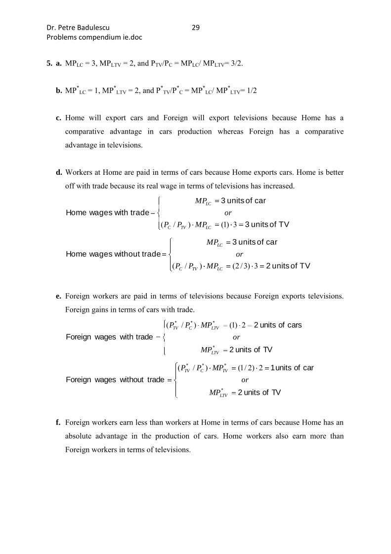
5. a. MPLC = 3, MPLTV = 2, and PTV/PC = MPLC/ MPLTV= 3/2.
b. MP*LC = 1, MP*
LTV = 2, and P*TV/P*
C = MP*LC/ MP*
LTV= 1/2
c. Home will export cars and Foreign will export televisions because Home has a
comparative advantage in cars production whereas Foreign has a comparative
advantage in televisions.
d. Workers at Home are paid in terms of cars because Home exports cars. Home is better
off with trade because its real wage in terms of televisions has increased.
TVofunits3
carofunits3
tradewithwagesHome
3)1()/( LCTVC
LC
MPPP
or
MP
TVofunits2
carofunits3
tradewithoutwagesHome
3)3/2()/( LCTVC
LC
MPPP
or
MP
e. Foreign workers are paid in terms of televisions because Foreign exports televisions.
Foreign gains in terms of cars with trade.
TVofunits2
carsofunits2
tradewithwagesForeign
*
*** 2)1()/(
LTV
LTVCTV
MP
or
MPPP
TVofunits2
carofunits1
tradewithoutwagesForeign
*
*** 2)2/1()/(
LTV
TVCTV
MP
or
MPPP
f. Foreign workers earn less than workers at Home in terms of cars because Home has an
absolute advantage in the production of cars. Home workers also earn more than
Foreign workers in terms of televisions.
Dr. Petre Badulescu 30 Problems compendium ie.doc
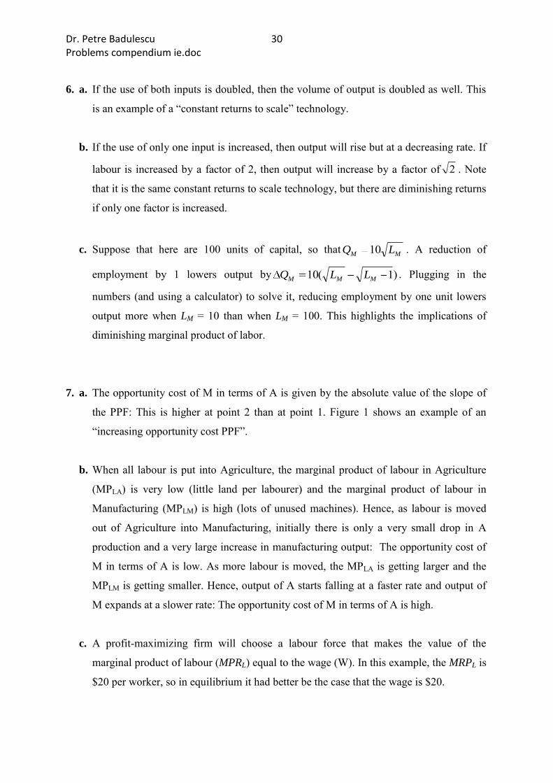
6. a. If the use of both inputs is doubled, then the volume of output is doubled as well. This
is an example of a “constant returns to scale” technology.
b. If the use of only one input is increased, then output will rise but at a decreasing rate. If
labour is increased by a factor of 2, then output will increase by a factor of 2 . Note
that it is the same constant returns to scale technology, but there are diminishing returns
if only one factor is increased.
c. Suppose that here are 100 units of capital, so thatMM LQ 10 . A reduction of
employment by 1 lowers output by )1(10 MMM LLQ . Plugging in the
numbers (and using a calculator) to solve it, reducing employment by one unit lowers
output more when LM = 10 than when LM = 100. This highlights the implications of
diminishing marginal product of labor.
7. a. The opportunity cost of M in terms of A is given by the absolute value of the slope of
the PPF: This is higher at point 2 than at point 1. Figure 1 shows an example of an
“increasing opportunity cost PPF”.
b. When all labour is put into Agriculture, the marginal product of labour in Agriculture
(MPLA) is very low (little land per labourer) and the marginal product of labour in
Manufacturing (MPLM) is high (lots of unused machines). Hence, as labour is moved
out of Agriculture into Manufacturing, initially there is only a very small drop in A
production and a very large increase in manufacturing output: The opportunity cost of
M in terms of A is low. As more labour is moved, the MPLA is getting larger and the
MPLM is getting smaller. Hence, output of A starts falling at a faster rate and output of
M expands at a slower rate: The opportunity cost of M in terms of A is high.
c. A profit-maximizing firm will choose a labour force that makes the value of the
marginal product of labour (MPRL) equal to the wage (W). In this example, the MRPL is
$20 per worker, so in equilibrium it had better be the case that the wage is $20.
Dr. Petre Badulescu 31 Problems compendium ie.doc
d. Because PMMPLM = W = PAMPLA in equilibrium, MPLA > MPLM because PM > PA.
Since wages equalize across the industries, the industry with the lower price per unit of
output must have the higher marginal productivity of labour.
e. The value of the marginal product of labour is $40, and workers are being paid only
$25. This means that revenues could be expanded by more than costs if another worker
is hired. Hence, you are employing too few workers.
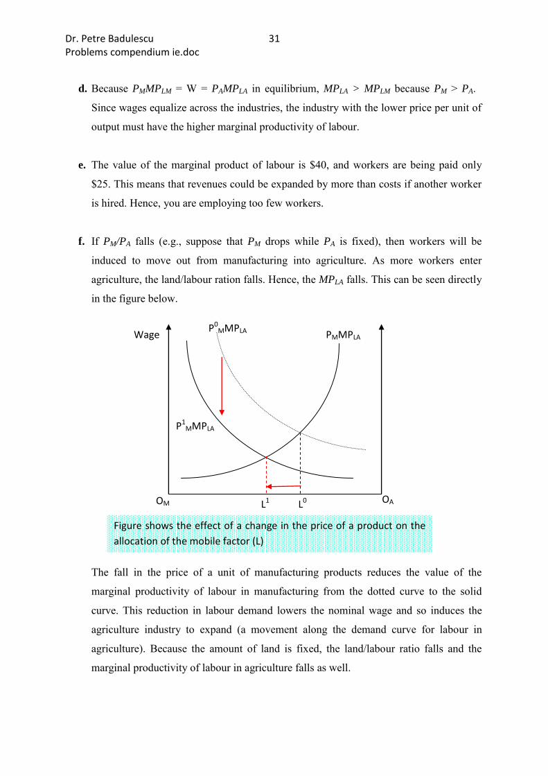
f. If PM/PA falls (e.g., suppose that PM drops while PA is fixed), then workers will be
induced to move out from manufacturing into agriculture. As more workers enter
agriculture, the land/labour ration falls. Hence, the MPLA falls. This can be seen directly
in the figure below.
The fall in the price of a unit of manufacturing products reduces the value of the
marginal productivity of labour in manufacturing from the dotted curve to the solid
curve. This reduction in labour demand lowers the nominal wage and so induces the
agriculture industry to expand (a movement along the demand curve for labour in
agriculture). Because the amount of land is fixed, the land/labour ratio falls and the
marginal productivity of labour in agriculture falls as well.
Wage
OA OM L1 L0
P1MMPLA
P0MMPLA
PMMPLA
Figure shows the effect of a change in the price of a product on the
allocation of the mobile factor (L)
Dr. Petre Badulescu 32 Problems compendium ie.doc
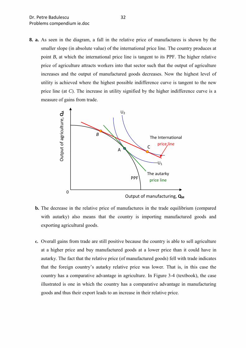
8. a. As seen in the diagram, a fall in the relative price of manufactures is shown by the
smaller slope (in absolute value) of the international price line. The country produces at
point B, at which the international price line is tangent to its PPF. The higher relative
price of agriculture attracts workers into that sector such that the output of agriculture
increases and the output of manufactured goods decreases. Now the highest level of
utility is achieved where the highest possible indifference curve is tangent to the new
price line (at C). The increase in utility signified by the higher indifference curve is a
measure of gains from trade.
b. The decrease in the relative price of manufactures in the trade equilibrium (compared
with autarky) also means that the country is importing manufactured goods and
exporting agricultural goods.
c. Overall gains from trade are still positive because the country is able to sell agriculture
at a higher price and buy manufactured goods at a lower price than it could have in
autarky. The fact that the relative price (of manufactured goods) fell with trade indicates
that the foreign country’s autarky relative price was lower. That is, in this case the
country has a comparative advantage in agriculture. In Figure 3-4 (textbook), the case
illustrated is one in which the country has a comparative advantage in manufacturing
goods and thus their export leads to an increase in their relative price.
The autarky
price line PPF
The International
price line
Ou
tpu
t o
f ag
ricu
ltu
re, Q
A
C
B
A
U2
U1
0 Output of manufacturing, QM

Dr. Petre Badulescu 33 Problems compendium ie.doc
9. a. Rental on land can be calculated as follows:
TR
LWWWQPPP
R
R
T
AAAAA
T
T )/()/(
%5.12125.0100
50)05.0(150)01.0(or
T
T
R
R.
Recalling that the price of manufacturing remained constant, we get the rental on capital
as
KR
LW
W
W
R
R
K
LWQR
M
M
M
MMMM
0
%101.050
100)05.0( orM
M
R
R.
b. Because the 10% increase in the price of agriculture, the real rental on land rose
whereas the real rental on capital fell. Therefore, landowners are better off because the
percentage increase in the rental on land is greater than the percentage increase in the
price of agriculture, whereas the price of manufacture is constant. Capital owners are
worse off in terms of their ability to purchase both manufacture and agriculture because
the rental to capital has fallen.
ATTAAMM PRRPPWWRR inincreaseanfor,///0/
c. Assuming that the decrease in the price of manufactures leads to a fall in wage by 5%,
capital owners would be worse off because the rental on capital would decrease (20%)
more than the drop in the price of manufacturing (10%). Landowners would be better
off as the rental on land rises (10%). The effect on labor is ambiguous because although
the percentage of wage decrease is less than the percentage fall in price of
manufacturing, labour loses in terms of their ability to purchase agriculture.
Real rental on capital
falls
Change in real wage is ambiguous
Real rental on land
rises

Dr. Petre Badulescu 34 Problems compendium ie.doc
The rental on capital is found by calculating the following:
KR
LWWWQPPP
R
R
M
MMMMM
M
M )/()/(
%2020.050
100)05.0(150)1.0(or
M
M
R
R
Although the rental on land is
T
LWQR AA
T
0 →TR
LW
W
W
R
R
T
A
T
T
%5,2025.01005005,0 or
T
T
R
R.
Putting it together we get
MTTMMMM PRRWWPPRR indecreaseafor,/0///
10. a. In the absence of trade, the relative price of autos is the slope (in absolute value) of the
line tangent to the PPF and Homes indifference curve.
b. See the diagrams below. Autarky state is displayed in dotted lines, and trade state is
displayed in solid lines. Home has the higher autarky relative price of autos and so it is
the exporter of bananas. Home’s supply of bananas increase and its supply of autos
decreases, whereas the opposite is true in Foreign. Home’s consumption of bananas is
less than its supply of bananas, and its consumption of autos is greater than its supply of
autos. The opposite is true in Foreign.
Real rental on capital falls
Change in the real wage is ambiguous
Real rental on land rises

Dr. Petre Badulescu 35 Problems compendium ie.doc
c. The rental price of capital falls in Home. As labour is pulled out of auto production, the
marginal product of capital, MPK, falls. Because
AKK PRMP /
the income of a unit of capital has fallen relative to the price of autos. Now notice that
A
K
B
A
B
K
P
R
P
P
P
R.
Because PA/PB goes down when the country trades, and because RK/PA falls as well, the
nominal earnings of a unit of capital will buy less of both goods!
The relative price of autos goes up for Foreign, and so the argument for Home applies
here but in reverse. The rental on capital rises in Foreign.
d. The demand for land in Home rises as the country increases its production of bananas.
The marginal product of land rises as labour is moved from auto production into banana
production. The value of the marginal product of land is the demand curve for land.
e. Because global resources are used more efficiently, both countries can consume more
than they did when they were not trading. Because the country gains from trade means
that winners win more than losers lose, the winners could compensate the losers and
everyone could be made better off.
1
B
1
B
DS
1
A
1
A
DS
2
BS
2
BD
2
AS 2
AD
2
BS
2
BD
2
AD 2
AS
0 0
Bananas Bananas
Autos Autos
Home Foreign
Figure: Trade versus Autarky in Home and Foreign
Dr. Petre Badulescu 36 Problems compendium ie.doc
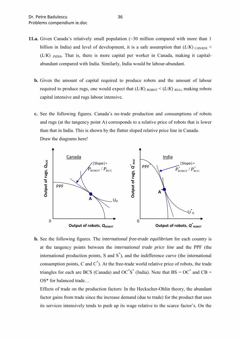
11.a. Given Canada’s relatively small population (~30 million compared with more than 1
billion in India) and level of development, it is a safe assumption that (L/K) CANADA <
(L/K) INDIA. That is, there is more capital per worker in Canada, making it capital-
abundant compared with India. Similarly, India would be labour-abundant.
b. Given the amount of capital required to produce robots and the amount of labour
required to produce rugs, one would expect that (L/K) ROBOT < (L/K) RUG, making robots
capital intensive and rugs labour intensive.
c. See the following figures. Canada’s no-trade production and consumptions of robots
and rugs (at the tangency point A) corresponds to a relative price of robots that is lower
than that in India. This is shown by the flatter sloped relative price line in Canada.
Draw the diagrams here!
b. See the following figures. The international free-trade equilibrium for each country is
at the tangency points between the international trade price line and the PPF (the
international production points, S and S*), and the indifference curve (the international
consumption points, C and C*). At the free-trade world relative price of robots, the trade
triangles for each are BCS (Canada) and OC*S* (India). Note that BS = OC* and CB =
OS* for balanced trade…
Effects of trade on the production factors: In the Heckscher-Ohlin theory, the abundant
factor gains from trade since the increase demand (due to trade) for the product that uses
its services intensively tends to push up its wage relative to the scarce factor’s. On the
PPF*
PPF
U0
U*0
A
A*
|Slope|=
RUGROBOT PP /
0 0
Ou
tpu
t o
f ru
gs, Q
* RU
G
Ou
tpu
t o
f ru
gs, Q
RU
G
Output of robots, Q*ROBOT Output of robots, QROBOT
Canada India
|Slope|=** / RUGROBOT PP

Dr. Petre Badulescu 37 Problems compendium ie.doc
other hand, the scarce factor loses from trade since consumers are now able to import
from the other country the product that uses the scarce factor intensively. This means
that local production of that product will drop and demand for its services will decline.
Here? In Canada, capital owners (the abundant factor) gain from trade, while labour (the
scarce factor) loses from trade. In India, labour (the abundant factor) gain from trade,
while capital (the scarce factor) loses from trade.
12. a. WLC /RKC > WLS/RKS (and thus LC/KC > LS/KS) implies that shoes are capital intensive.
This is certainly possible as shown in the New Balance application.
b. For computers:
)/(
50/)}50)(/(100%)0{(/})/()/{(/
WW
WW
RKWLWWQPPPRR CCCCCC
For shoes:
)95/5)(/(95/50
95/)}5)(/(100%)50{(/})/()/{(/
WW
WW
RKWLWWQPPPRR SSSSSS
Substituting the computer equation into the shoes equation:
The international free-trade equilibrium relative price of robots, (PROBOT/PRUG)W, is given by the absolute value of the slope of the world price line (the red line) – the tangent, also called the consumption possibilities frontier. This equilibrium relative price is determined by the international market for robots where the import demand equals the export supply.
S* U*
1
U*0
U1
U0
PPF*
PPF
O A*
Exports B S
C*
C
A Imports
Exports
Imports
0 0
Ou
tpu
t o
f ru
gs, Q
* RU
G
Ou
tpu
t o
f ru
gs, Q
RU
G
Output of robots, Q*ROBOT Output of robots, QROBOT
Canada India World price line, |slope| =
(PROBOT/PRUG)W

Dr. Petre Badulescu 38 Problems compendium ie.doc
%6.55556.0)90/50(/
95/50)95/51(/)95/5)(/(95/50/orRR
RRRRRR
This implies: %.6.55// RRWW
As seen in the percentage change calculation for the rental of capital in the shoes
industry, the magnitude of the changes are equal (with opposite sign).
c. Because the increase in capital returns exceeds the price changes in both industries,
capital gains in real terms. Similarly, because there is a decrease in wage and the prices
of the outputs stayed the same or increased, labour loses in real terms. This is consistent
with the Stolper-Samuelson theorem: In the long run, when all factors are mobile, an
increase in the relative price of a good will cause the real earnings of labour and capital
to move in opposite directions, with a rise in the real earnings of the factor used
intensively in the industry whose relative price went up and a decrease in the real
earnings of the other factor.
13. Because the United States is relatively abundant in skilled labour and scarce in unskilled
labour, as predicted by the Heckscher-Ohlin model the U. S. imports unskilled-labour–
intensive goods such as apparel, footwear, furniture, and toys.
Assuming pharmaceutical products use skilled labour, U. S. imports of these goods are
contrary to the prediction of the model. Both skilled labour and capital are used
intensively in the production of aircraft, and given that the United States has abundance
in both factors, the export of this good supports the Heckscher-Ohlin model. However,
the model is unsupported by the import of electric machinery and vehicles as both goods
also use intensively skilled labour and capital. The export of cotton is also likely to
contradict the Heckscher-Ohlin model because the United States is relatively land
scarce.
Dr. Petre Badulescu 39 Problems compendium ie.doc
14. a. Airplanes are capital intensive relative to shirts because the capital/labour ratio is 5/3,
which is greater than the capital/labour ratio in shirts = 1.
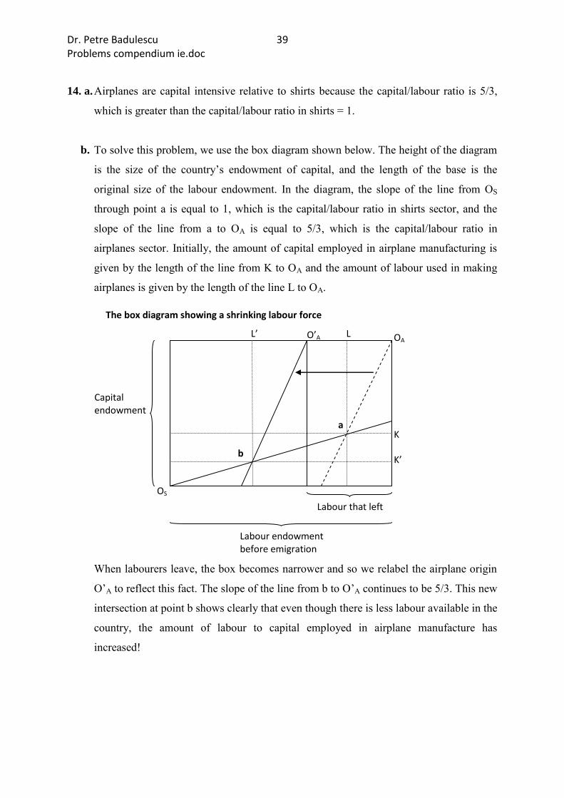
b. To solve this problem, we use the box diagram shown below. The height of the diagram
is the size of the country’s endowment of capital, and the length of the base is the
original size of the labour endowment. In the diagram, the slope of the line from OS
through point a is equal to 1, which is the capital/labour ratio in shirts sector, and the
slope of the line from a to OA is equal to 5/3, which is the capital/labour ratio in
airplanes sector. Initially, the amount of capital employed in airplane manufacturing is
given by the length of the line from K to OA and the amount of labour used in making
airplanes is given by the length of the line L to OA.
When labourers leave, the box becomes narrower and so we relabel the airplane origin
O’A to reflect this fact. The slope of the line from b to O’A continues to be 5/3. This new
intersection at point b shows clearly that even though there is less labour available in the
country, the amount of labour to capital employed in airplane manufacture has
increased!
The box diagram showing a shrinking labour force
O’A
Labour that left
b
L L’
K’
a K
Labour endowment before emigration
Capital endowment
OA
OS
Dr. Petre Badulescu 40 Problems compendium ie.doc
c. Let QA denote the output of airplanes and QS denote the output of shirts. Let K be the
country’s endowment of capital, and let L be the country’s endowment of labour. Using
the production data in the problem we have
AS QQK 52 and
AS QQL 32 .
Doing a little algebra, we find that
435 KL
QS and 2
KLQA .
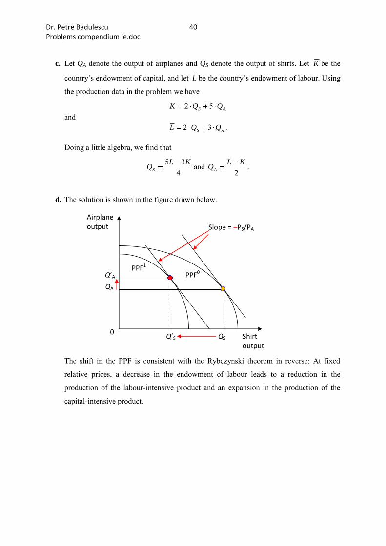
d. The solution is shown in the figure drawn below. The shift in the PPF is consistent with the Rybczynski theorem in reverse: At fixed
relative prices, a decrease in the endowment of labour leads to a reduction in the
production of the labour-intensive product and an expansion in the production of the
capital-intensive product.
PPF1 PPF0
Q’S
Q’A
Airplane output
Shirt output
0 QS
QA
Slope = –PS/PA

Dr. Petre Badulescu 41 Problems compendium ie.doc
15. a. Gains from trade in the following graph are analogous to consumer and producer
surplus in the conventional supply and demand setting. In this case, Home employers
are willing to pay up to W for the marginal product of labour that they obtain for W;
thus the gains to the Home country are illustrated by the horizontally striped triangle.
Similarly, the immigrating Foreign workers are willing to supply their marginal product
for a lower wage in the Foreign country (W*) but receive a higher wage in the Home
country (W**).
b. Gains to Foreign (including foreign emigrants) are represented by the vertically striped
triangle. Given positive gains to both countries, total gains from immigration are also
positive in this model.
c. i.) The value of output is the area under the value of marginal product of labour curve –
the demand curve for labour. Given the strait line, this area can be calculated as
25·50 + (1/2) · [(30 – 25) · (150 –100)] = 1375.
Hence, the increase in the value of output is the increase in this total area.
ii.) The increase in output value was 1375, but of this 25 · 50 = 1250 is paid to foreigners
who have entered the country. Hence, the total gain to the country is 125.
iii.) Home-specific factors gain from access lower cost labour. They receive the 125
calculated in the previous problem plus the direct effect of paying the same workers
less to the tune of 5 · 100 = 500, so the total gain to specific factors is 625.
B
A
25
50
5
5
← *L L →
W**
W’’
World amount of labor
W*=20
W’=25
W=30 A
B
A*
L=100 L’=150 0* 0
Home
wage
Foreign
wage
Wage, W

Dr. Petre Badulescu 42 Problems compendium ie.doc
2. Modern international trade theory: scale economies and imperfections
1. With increasing returns to scale, countries benefit from trade due to the potential to
reduce their average costs by expanding their outputs through selling in a larger market.
2. The firm’s total average cost is (€2 · Q + €100)/Q. When Q = 10, ATC = €12. A firm
selling 10 units must be getting a price of €12 to break even.
3. a. The effect of increasing the number of products in the market is shown in the figure
below. The solid curve D/N is demand per firm when each firm charges the same price
before the increase in the number of products, and the dotted line labelled D/N’ is the
curve after the increase in the products. The solid line labelled d is demand before the
increase, and the broken curve labelled d’ is demand after the increase.
b. The shift in the D/N curve is simple: The same amount of demand is split over a larger
number of firms. The shift in the d curve is more complicated. The curve shifts down
because the more products in the market, the less demand there is for any given product.
It also becomes flatter because with increased product choice consumers become more
sensitive to price differences across products.
0 Quantity
Price
d’
d
D/N’ D/N
Dr. Petre Badulescu 43 Problems compendium ie.doc
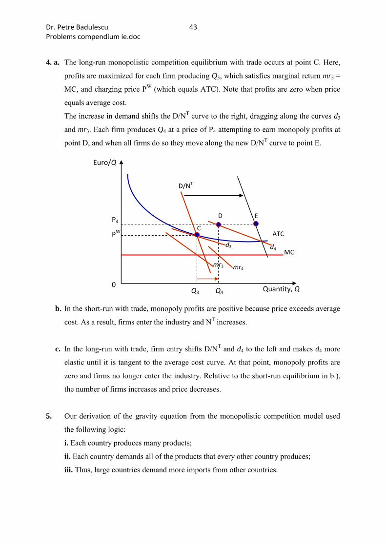
4. a. The long-run monopolistic competition equilibrium with trade occurs at point C. Here,
profits are maximized for each firm producing Q3, which satisfies marginal return mr3 =
MC, and charging price PW (which equals ATC). Note that profits are zero when price
equals average cost.
The increase in demand shifts the D/NT curve to the right, dragging along the curves d3
and mr3. Each firm produces Q4 at a price of P4 attempting to earn monopoly profits at
point D, and when all firms do so they move along the new D/NT curve to point E.
b. In the short-run with trade, monopoly profits are positive because price exceeds average
cost. As a result, firms enter the industry and NT increases.
c. In the long-run with trade, firm entry shifts D/NT and d4 to the left and makes d4 more
elastic until it is tangent to the average cost curve. At that point, monopoly profits are
zero and firms no longer enter the industry. Relative to the short-run equilibrium in b.),
the number of firms increases and price decreases.
5. Our derivation of the gravity equation from the monopolistic competition model used
the following logic:
i. Each country produces many products;
ii. Each country demands all of the products that every other country produces;
iii. Thus, large countries demand more imports from other countries.
ATC
d3
mr3
Q4
E
d4
mr4
D
Q3
C
D/NT
P4
PW
Euro/Q
0 Quantity, Q
MC

Dr. Petre Badulescu 44 Problems compendium ie.doc
The Heckscher-Ohlin (H-O) model assumes perfect competition. Therefore, each
country produces many products. However, in the H-O model not all products produced
in other countries (in autarky) are imported under trade. Rather, because products are
not differentiated, only those identical products with a lower relative price abroad are
imported, and countries specialize in the product that uses their abundant factor
intensively. Hence, larger countries do not necessarily demand more imports from other
countries.
6. a. The expected level of trade between the United States and France is 93(14,270 · 2,635) /
5, 5441.25 = $73,098 billion. The expected level of trade between the United States and
Italy is 93(2,090 · 14,270) / 6, 2291.25 = $50,122 billion.
(Note: These numbers are larger than is realistic because we are using the gravity
equation estimated on the United States and Canada state/provincial trade, rather than
the equation estimated on international trade.)
b. The expected level of trade between Italy and France is 93(2,635 · 2,090) / 6941.25 =
$143,784 billion. This number is so large because it reflects the short distance between
the two countries. In particular, this number is larger than the predicted amount of trade
between the United States and Italy, as calculated in part (a).
7. Yes. Wine is differentiated to some extent merely by where it is produced. In principle,
this is enough to generate intra-industry trade: People may consume both wines from
California and from France merely for variety
Dr. Petre Badulescu 45 Problems compendium ie.doc
3. International trade policy
1. a. The firm would be selling its product in your market at less than the normal price.
Normal price would mean the price in the exporting country’s market, the price in a
third country, or the average cost of production.
b. This is an example of a free trade agreement, which is allowed under Article XXIV of
the GATT.
c. “Normal trade relations” perhaps better conveys the actual meaning of “most favoured
nation status”, which is the principle of non-discrimination.
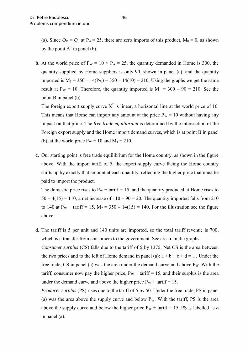
2. a. The import demand curve, M, shows the relationship between the world price of a
product and the quantity of imports demanded by the country consumers. We derive it
from the domestic demand curve (D) and the domestic supply curve (S), i.e.
M = demanded quantity – supplied quantity: M = QD – QS.
Home’s import demand curve for peanuts is
M = (400 – 10P) – (50 + 4P) = 350 – 14P.
The figure above shows the domestic and import markets for peanuts in Home. The no-
trade equilibrium is at point A, where QD equals QS, which determines Home’s autarky
equilibrium price PA = 25, and its autarky equilibrium quantity of Q0 = 150. See panel
Import, M
Price Price
PW
M2 = 140
M1 = 210
c B
b
c a
140
15 X*+ tariff
M
Foreign export supply, X*
Q 210 300
(b) Home import market (a) Home market
A’ A
D
S
10
25
150 0 0 50 90 400
40
PWORLD+ tariff
PWORLD
d
Deadweight loss due to the tariff
b + d
Dr. Petre Badulescu 46 Problems compendium ie.doc
(a). Since QD = QS at PA = 25, there are zero imports of this product, M0 = 0, as shown
by the point A’ in panel (b).
b. At the world price of PW = 10 < PA = 25, the quantity demanded in Home is 300, the
quantity supplied by Home suppliers is only 90, shown in panel (a), and the quantity
imported is M1 = 350 – 14(PW) = 350 – 14(10) = 210. Using the graphs we get the same
result at PW = 10. Therefore, the quantity imported is M1 = 300 – 90 = 210. See the
point B in panel (b).
The foreign export supply curve X* is linear, a horizontal line at the world price of 10.
This means that Home can import any amount at the price PW = 10 without having any
impact on that price. The free trade equilibrium is determined by the intersection of the
Foreign export supply and the Home import demand curves, which is at point B in panel
(b), at the world price PW = 10 and M1 = 210.
c. Our starting point is free trade equilibrium for the Home country, as shown in the figure
above. With the import tariff of 5, the export supply curve facing the Home country
shifts up by exactly that amount at each quantity, reflecting the higher price that must be
paid to import the product.
The domestic price rises to PW + tariff = 15, and the quantity produced at Home rises to
50 + 4(15) = 110, a net increase of 110 – 90 = 20. The quantity imported falls from 210
to 140 at PW + tariff = 15. M2 = 350 – 14(15) = 140. For the illustration see the figure
above.
d. The tariff is 5 per unit and 140 units are imported, so the total tariff revenue is 700,
which is a transfer from consumers to the government. See area c in the graphs.
Consumer surplus (CS) falls due to the tariff of 5 by 1375. Net CS is the area between
the two prices and to the left of Home demand in panel (a): a + b + c + d = … Under the
free trade, CS in panel (a) was the area under the demand curve and above PW. With the
tariff, consumer now pay the higher price, PW + tariff = 15, and their surplus is the area
under the demand curve and above the higher price PW + tariff = 15.
Producer surplus (PS) rises due to the tariff of 5 by 50. Under the free trade, PS in panel
(a) was the area above the supply curve and below PW. With the tariff, PS is the area
above the supply curve and below the higher price PW + tariff = 15. PS is labelled as a
in panel (a).
Dr. Petre Badulescu 47 Problems compendium ie.doc
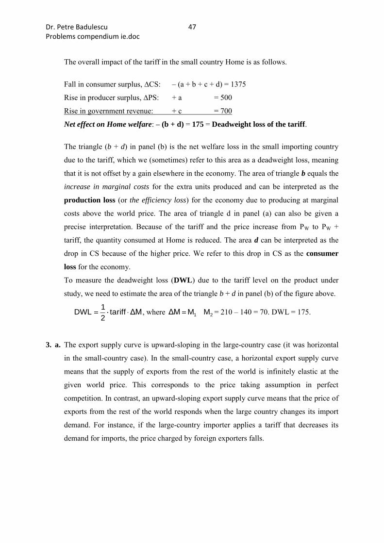
The overall impact of the tariff in the small country Home is as follows.
Fall in consumer surplus, ∆CS: – (a + b + c + d) = 1375
Rise in producer surplus, ∆PS: + a = 500
Rise in government revenue: + c = 700
Net effect on Home welfare: – (b + d) = 175 = Deadweight loss of the tariff.
The triangle (b + d) in panel (b) is the net welfare loss in the small importing country
due to the tariff, which we (sometimes) refer to this area as a deadweight loss, meaning
that it is not offset by a gain elsewhere in the economy. The area of triangle b equals the
increase in marginal costs for the extra units produced and can be interpreted as the
production loss (or the efficiency loss) for the economy due to producing at marginal
costs above the world price. The area of triangle d in panel (a) can also be given a
precise interpretation. Because of the tariff and the price increase from PW to PW +
tariff, the quantity consumed at Home is reduced. The area d can be interpreted as the
drop in CS because of the higher price. We refer to this drop in CS as the consumer
loss for the economy.
To measure the deadweight loss (DWL) due to the tariff level on the product under
study, we need to estimate the area of the triangle b + d in panel (b) of the figure above.
ΔMtariff2
1DWL , where 21 MMΔM = 210 – 140 = 70. DWL = 175.
3. a. The export supply curve is upward-sloping in the large-country case (it was horizontal
in the small-country case). In the small-country case, a horizontal export supply curve
means that the supply of exports from the rest of the world is infinitely elastic at the
given world price. This corresponds to the price taking assumption in perfect
competition. In contrast, an upward-sloping export supply curve means that the price of
exports from the rest of the world responds when the large country changes its import
demand. For instance, if the large-country importer applies a tariff that decreases its
demand for imports, the price charged by foreign exporters falls.

Dr. Petre Badulescu 48 Problems compendium ie.doc
b. The tariff shifts the export supply curve from X* to X*+ t. The X*+ t curve intersects
import demand curve M at point C, which establishes the new equilibrium. As a result,
the price in the importing country increases from PWORLD to P* + t, and the Foreign price
falls from PW to P*. The deadweight loss at importing country is the area of the triangles
(b + d), and the importing country also has a terms-of-trade, t-o-t, gain of area e.
The overall impact of the tariff in the large country is obtained by summing the change
in consumer surplus (CS), producer surplus (PS), and government revenue:
Fall in consumer surplus, ∆CS: – (a + b + c + d)
Rise in producer surplus, ∆PS: + a
Rise in government revenue: + (c + e) ___
Net effect on large country welfare: + e – (b + d)
The triangle (b + d) is the deadweight loss due to the tariff (just as it is for a small
country). But for the large country there is also a source of gain – the area e, a precise
measure of the t-o-t for the importer – that offsets this deadweight loss. If e > (b + d),
then the importing country is better off due to the tariff; if e < (b + d), then the
importing country is worse off.
Foreign loses the area (e + f), so the net loss in the world welfare is the area of the
triangles (b + d + f).
Price Price
PW
f
a
b + d
D2 Q2W
C* P*
e
C P*+ t
P*
S1 S2 D1
PWORLD B*
S
Q1W
M
X*
Q Quantity
(b) World market (a) Importer’s domestic market
A’ A
D
0 0
b
c
X*+ t
d
e

Dr. Petre Badulescu 49 Problems compendium ie.doc
c. Refer to the figure in the previous problem 2: In the small-country case (flat export
supply curve), a tariff increases the amount that consumers pay by exactly the amount
of the tariff and foreign exporters are paid the original world price, PW; the difference is
collected by the domestic government as tax revenue.
Refer to the Figure above (Problem 3.a): With an upward-sloping export supply curve
(in the large-country case) foreign exporters reduce their price due to a tariff; that is,
foreign exporters receive less than they did prior to the tariff. Domestic consumers pay
more than before, but by less than the full amount of the tariff. Again, the difference
between what consumers pay and what Foreign exporters receive is the amount of the
tariff, t, collected by the domestic government. In the large-country case, the incidence
of the tariff is shared by domestic consumers and foreign producers. Moreover, a
steeper foreign export supply curve implies that foreign exporters absorb more of the
price increase due to the tariff.
4. a. The elasticity of the export supply curve is related to its steepness. The steeper the
supply curve, the lower the elasticity. When the supply curve is very steep, the more the
incidence of the tariff falls on the exporting country. The more the tariff is borne by the
foreigners, the larger the tariff.
b. This is the large-country case. The optimal tariff is determined as:
*
1
xEttariffoptimal , where *
xE is the Foreign export supply elasticity.
c. The figure below shows tariffs and welfare for a large importing country.
Prohibitive
tariff
A
B’ t-o-t gain is less than
deadweight loss
t-o-t gain exceeds
deadweight loss
Optimal
tariff
Free trade B
C
No trade
Tariff 0
Importer’s
welfare
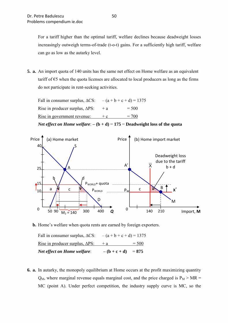
Dr. Petre Badulescu 50 Problems compendium ie.doc
For a tariff higher than the optimal tariff, welfare declines because deadweight losses
increasingly outweigh terms-of-trade (t-o-t) gains. For a sufficiently high tariff, welfare
can go as low as the autarky level.
5. a. An import quota of 140 units has the same net effect on Home welfare as an equivalent
tariff of €5 when the quota licenses are allocated to local producers as long as the firms
do not participate in rent-seeking activities.
Fall in consumer surplus, ∆CS: – (a + b + c + d) = 1375
Rise in producer surplus, ∆PS: + a = 500
Rise in government revenue: + c = 700
Net effect on Home welfare: – (b + d) = 175 = Deadweight loss of the quota
b. Home’s welfare when quota rents are earned by foreign exporters. Fall in consumer surplus, ∆CS: – (a + b + c + d) = 1375
Rise in producer surplus, ∆PS: + a = 500
Net effect on Home welfare: – (b + c + d) = 875
6. a. In autarky, the monopoly equilibrium at Home occurs at the profit maximizing quantity
QM, where marginal revenue equals marginal cost, and the price charged is PM > MR =
MC (point A). Under perfect competition, the industry supply curve is MC, so the
Price Price
PW
M2 = 140
c B
b
c a
140
15
X
M
X*
Q Import, M 210 300
(b) Home import market (a) Home market
A’ A
D
S
10
25
0 0 50 90 400
40
PWORLD+ quota
PWORLD
d
Deadweight loss due to the tariff
b + d

Dr. Petre Badulescu 51 Problems compendium ie.doc
autarky equilibrium would occur where demand equals supply (point B), at the quantity
QC and the price PC.
Notice that we assume that cost conditions facing the competitive firms are the same as those facing the monopolist, so the industry supply curve under perfect competition is equal to the monopolist’s marginal cost curve MC.
Refer to the figure above: Consumer surplus is the area under the demand curve D and
above the market price, and producer surplus is the area above the marginal cost curve
MC and below the market price. Under perfect competition, consumer surplus is PCBE,
where E is the intersection of the demand curve with the vertical axis. Producer surplus
is PCBPMC, where PMC is the intersection of the marginal cost curve with the vertical
axis. Total surplus is thus represented by the triangle PMCBE.
b. Consumer surplus is the triangle PMAE. Producer surplus is the same as the profits
earned by the monopolist. To measure this, label the point in the figure above where the
MR curve intersects MC at point B´. For selling the units between zero and QM,
marginal costs rise along the MC curve, up to B´. The monopolist earns the difference
between the price PM and MC for each unit sold. Label the difference between the price
and the MC curve as producer surplus, or profits, given that there is no fast cost.
Producer surplus is represented by the trapezoid PMAB´PMC. Referring to the figure
above part (a):
Total surplus is represented by the trapezoid EAB´PMC.
c. Refer to the figure from part (a): This is called the deadweight loss due to monopoly,
and is represented by the triangle ABB´. It is called a deadweight loss because it is a
loss that is not gained by any other party.
B’
PMC
E
A
B PC
PM
QC QM
Perfect Competition equilibrium
Marginal
cost, MC
0
Euro/ Q
Quantity, Q
Home
demand, D
Marginal
revenue, MR
Monopoly equilibrium

Dr. Petre Badulescu 52 Problems compendium ie.doc
7. a. Home is treated as a small country, which means that it faces the fixed world price of
PW. At PW, Foreign will supply any quantity of imports, because Home is a “price-
taker”, the Foreign export supply X* is perfectly elastic. Likewise, the Home monopolist
behaves as a “price-taker” at the price of PW (because it is able to export at the world
price) but cannot charge any more than that price at Home. If it charged a higher price,
Home consumers would import the product instead. Therefore, X* is also the new
demand curve facing the Home monopolist: the original no-trade demand of D no
longer applies.
Because the new demand curve facing the Home monopolist is perfectly inelastic (a
horizontal line at PW in the graph), the Home firm’s marginal curve is the same as the
demand curve, so X* = MR; the no-trade marginal revenue curve MR no longer applies.
To maximize profits under the new free-trade market conditions, the monopolist will set
MR = MC (point B I the figure below) and will supply S1 at the price PW. At the price
PW, Home consumers demand D1, which is more than the Home supply S1. The
difference between demand and supply is Home imports under international free trade,
or M1 = D1 – S1.
Because the Home monopolist now sets its price at marginal cost, the same free-trade
equilibrium holds under perfect competition.
b. Refer to the figure from part (a). The free-trade equilibrium under:
(i) Perfect competition has a Home consumer surplus of EB’PW = CS, and a producer
surplus of PWBPMC = PS. Gains from trade are represented by the shaded triangle.
(ii) Monopoly has a Home consumer surplus of EB’PW = CS, and a producer surplus of
PWBPMC = PS. This is identical to the free-trade surplus under perfect competition.
A’
X*= MR* B’
S1
B PW
PMC
E
A
PC
PM
D1 QM
MC
0
Euro/ Q
Quantity, Q
D MR
Gains from trade

Dr. Petre Badulescu 53 Problems compendium ie.doc
c. Home monopoly producer surplus in autarky equilibrium is represented by the trapezoid
PMAA’PMC. Gains from free-trade under Home monopoly are represented by the area
AB’BA’.
d. The area representing gains from trade is larger in part (c) than in part b. (i) and (ii).
This is because the opening of trade in the monopoly case eliminates the monopolist’s
ability to charge a price higher than the perfectly competitive price. As such, trade
additionally eliminates the deadweight loss associated with monopoly, making gains
from trade higher.
8. a. See the figure below. Note that the marginal revenue curve MR has been omitted to
avoid clustering up the diagram. The result is very similar to the perfect competition
small-country case. The tariff increases the domestic price, expanding the production
and the producer surplus by area a, and decreasing the consumption and the consumer
surplus by area (a + b + c + d). The tariff collects revenue c, so the total impact on
national welfare is – (b + d).
b. Because the quota does not allow imports to expand above the size of the quota when
the price on the domestic market rises, the Home firm has monopoly power. As shown
in the figure below, the quota that under perfect competition would lower imports by the
same amount as a tariff of size t has the effect of shifting the demand curve and
marginal revenue curve facing the monopolist to the left. The firm charges a mark-up
over its marginal cost that exceeds the size of the tariff t. As a result, the domestic price
with a quota PQ exceeds the domestic price with a tariff PW + t, so consumer surplus is
lower under quota than it is under a tariff.
c d a b
D1 S1
X*
PW + t
PW
D
Euro/ Q
Quantity, Q 0
MC
X*+ t
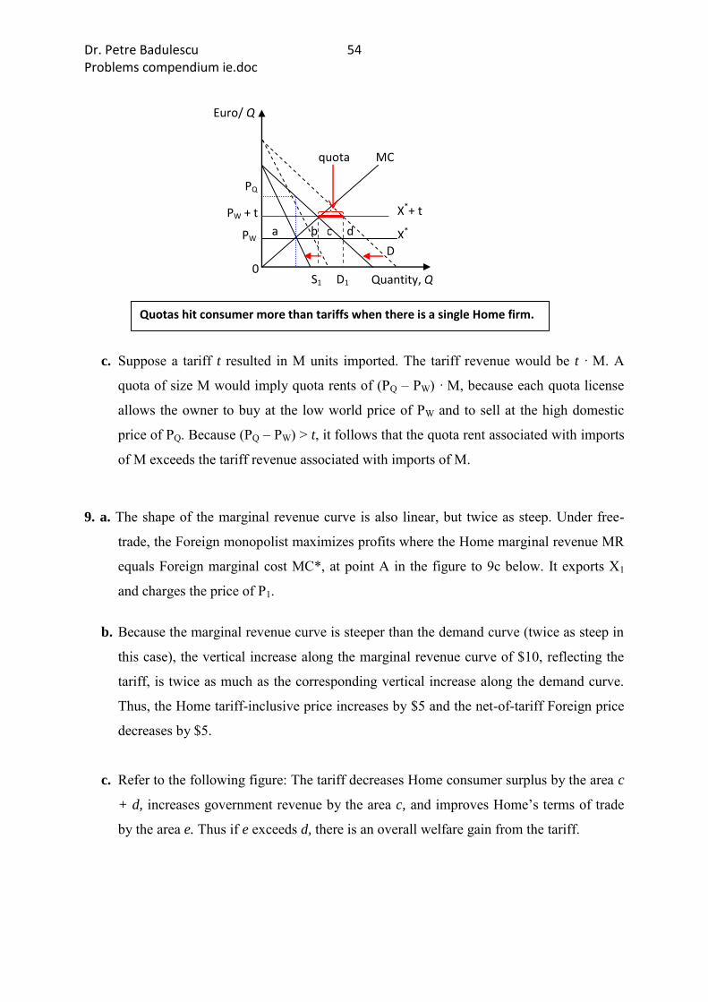
Dr. Petre Badulescu 54 Problems compendium ie.doc
c. Suppose a tariff t resulted in M units imported. The tariff revenue would be t · M. A
quota of size M would imply quota rents of (PQ – PW) · M, because each quota license
allows the owner to buy at the low world price of PW and to sell at the high domestic
price of PQ. Because (PQ – PW) > t, it follows that the quota rent associated with imports
of M exceeds the tariff revenue associated with imports of M.
9. a. The shape of the marginal revenue curve is also linear, but twice as steep. Under free-
trade, the Foreign monopolist maximizes profits where the Home marginal revenue MR
equals Foreign marginal cost MC*, at point A in the figure to 9c below. It exports X1
and charges the price of P1.
b. Because the marginal revenue curve is steeper than the demand curve (twice as steep in
this case), the vertical increase along the marginal revenue curve of $10, reflecting the
tariff, is twice as much as the corresponding vertical increase along the demand curve.
Thus, the Home tariff-inclusive price increases by $5 and the net-of-tariff Foreign price
decreases by $5.
c. Refer to the following figure: The tariff decreases Home consumer surplus by the area c
+ d, increases government revenue by the area c, and improves Home’s terms of trade
by the area e. Thus if e exceeds d, there is an overall welfare gain from the tariff.
quota
PQ
c d a b
D1 S1
X*
PW + t
PW D
Euro/ Q
Quantity, Q 0
MC
X*+ t
Quotas hit consumer more than tariffs when there is a single Home firm.

Dr. Petre Badulescu 55 Problems compendium ie.doc
10. a. Refer to the following figure: The threat of an antidumping duty causes the Foreign
firm to increase its price by t = P2 – P1. Consumer surplus decreases by the area (a + b)
b. A safeguard tariff would differ in two ways: (1) The Home government would collect
revenue on imports and (2) there would be a terms-of-trade gain for the Home country
because the incidence of the tariff would be shared by the Foreign monopolist. Both
differences reduce the amount of Home welfare loss under a tariff relative to a
threatened antidumping duty.
c. Despite their higher welfare costs, antidumping tariffs have a higher likelihood of being
implemented under U. S. trade law than safeguard tariffs. Because Home producers
benefit due to higher prices when there is even a threat of an antidumping duty, they
have an incentive to apply for this kind of protection.
B
P2 P1
e
A
Price
X2 X1
P3= P2 - t
0
Demand
t MC*
Marginal revenue
Foreign exports
MC* + t
c d
P1
P2 b
a
Q1
Price
0 Quantity
Demand
Quantity Q2

Dr. Petre Badulescu 56 Problems compendium ie.doc
11. If all markets are working perfectly, there is no reason why a potentially successful
fledgling industry cannot survive without government intervention. Let us consider the
two justifications for using an infant industry tariff. The first is that the industry will
learn over time, which will drive down its average costs to the point where it is
competitive; if credit markets were working perfectly, that industry could borrow
against future profitability to keep it in business until that time. The second justification
explicitly assumes a market imperfection: A positive externality in production implies
that the socially optimal level of infant industry output is above that determined by the
market equilibrium.
12. Positive externality exists when the increase in production by one firm generates
benefits to other firms by lowering industry costs. By imposing the tariff, the
government could nurture the infant industry because the increase in output allows the
firms to reduce their future costs by learning from each other. Without the protection,
each firm on its own would lack the incentive to invest in learning through increasing its
current production.
13. To the extent that the Home infant industry has market power, it is better to use a tariff
rather than a quota. The infant industry calculus weighs the benefits of future producer
surplus against current deadweight losses due to protection. Because deadweight losses
are greater under a quota due to maintaining Home market power, infant industry
protection has a better chance of being worthwhile by using a tariff.
14. a. There are unambiguous gains to the large exporting country. Not only do deadweight
losses decrease but terms-of-trade losses due to the subsidy are also diminished.
b. From our discussion of small-country tariffs, the optimal tariff level is zero. Hence, the
small food importer gains from reducing its tariff as deadweight losses decrease.
c. From our discussion of large-country tariffs, the optimal tariff level is positive because
(for small tariffs) terms-of-trade gains exceed deadweight losses. If we assume that the
(tariff-reducing) country was previously at its optimal tariff, then welfare is reduced by
cutting its tariff, but there is still an overall gain from the bilateral reduction in subsidies
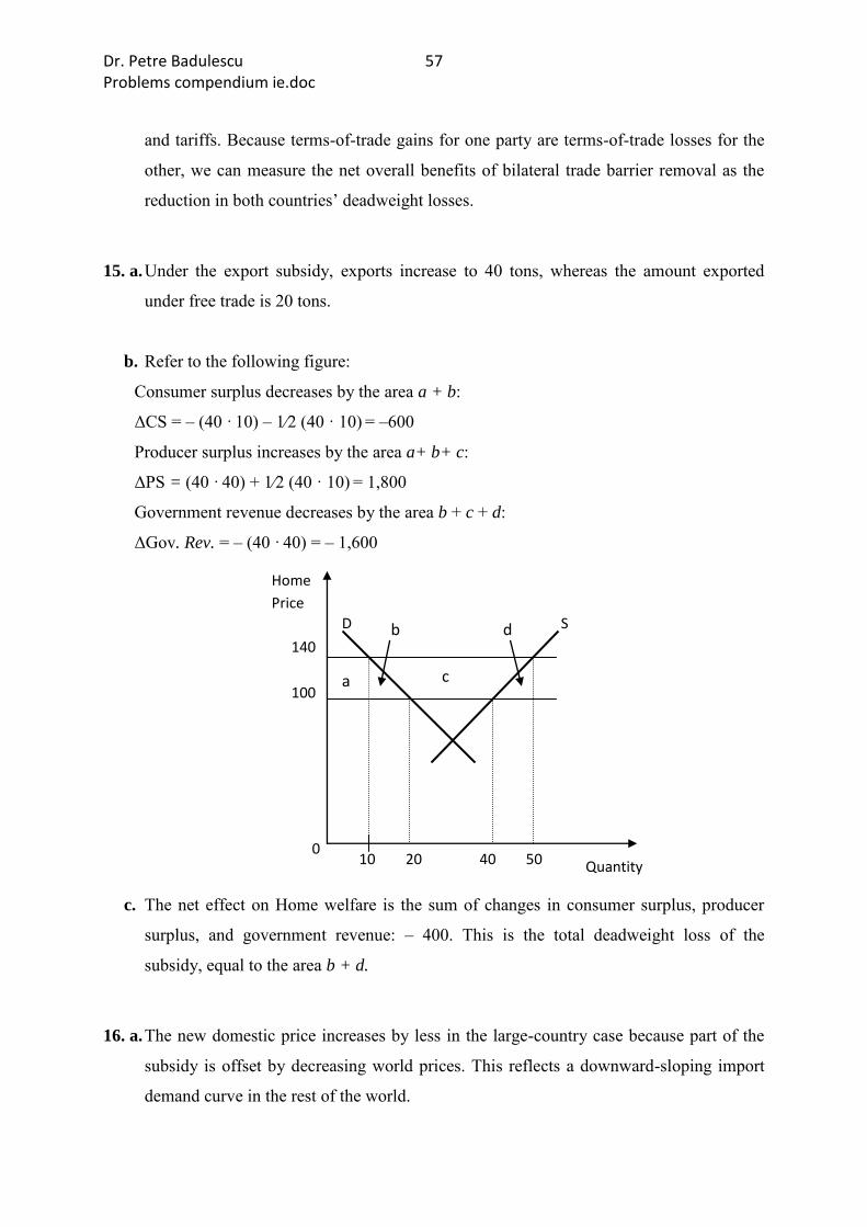
Dr. Petre Badulescu 57 Problems compendium ie.doc
and tariffs. Because terms-of-trade gains for one party are terms-of-trade losses for the
other, we can measure the net overall benefits of bilateral trade barrier removal as the
reduction in both countries’ deadweight losses.
15. a. Under the export subsidy, exports increase to 40 tons, whereas the amount exported
under free trade is 20 tons.
b. Refer to the following figure:
Consumer surplus decreases by the area a + b:
ΔCS = – (40 · 10) – 1⁄2 (40 · 10) = –600
Producer surplus increases by the area a+ b+ c:
ΔPS = (40 · 40) + 1⁄2 (40 · 10) = 1,800
Government revenue decreases by the area b + c + d:
ΔGov. Rev. = – (40 · 40) = – 1,600
c. The net effect on Home welfare is the sum of changes in consumer surplus, producer
surplus, and government revenue: – 400. This is the total deadweight loss of the
subsidy, equal to the area b + d.
16. a. The new domestic price increases by less in the large-country case because part of the
subsidy is offset by decreasing world prices. This reflects a downward-sloping import
demand curve in the rest of the world.
140
100
Home
Price
Quantity 0
50 40 10 20
D S
a
d
c
b

Dr. Petre Badulescu 58 Problems compendium ie.doc
b. Refer to the following figure:
Consumer surplus decreases by the area a + b:
ΔCS = – (20 · 12) – 1⁄2 (20 · 8) = – 320
Producer surplus increases by the area a + b + c:
ΔPS = (20 · 40) + 1⁄2 (20 · 8) = 880
Government revenue decreases by the area b + c + d + e:
ΔGov. Rev. = – (40 · 36) = – 1,440
c. The net decrease in welfare due to the subsidy is – 880. This is a larger loss than in the
small country because of Home’s terms-of-trade loss.
c
b d
a
80
120
100
Home
Price
Quantity 0
48 40 12 20
D S
e
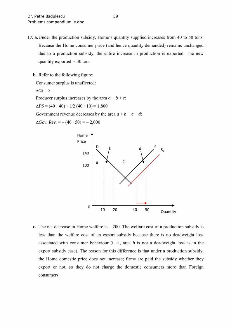
Dr. Petre Badulescu 59 Problems compendium ie.doc
17. a. Under the production subsidy, Home’s quantity supplied increases from 40 to 50 tons.
Because the Home consumer price (and hence quantity demanded) remains unchanged
due to a production subsidy, the entire increase in production is exported. The new
quantity exported is 30 tons.
b. Refer to the following figure:
Consumer surplus is unaffected: ∆CS = 0
Producer surplus increases by the area a + b + c:
∆PS = (40 · 40) + 1⁄2 (40 · 10) = 1,800
Government revenue decreases by the area a + b + c + d:
∆Gov. Rev. = – (40 · 50) = – 2,000
c. The net decrease in Home welfare is – 200. The welfare cost of a production subsidy is
less than the welfare cost of an export subsidy because there is no deadweight loss
associated with consumer behaviour (i. e., area b is not a deadweight loss as in the
export subsidy case). The reason for this difference is that under a production subsidy,
the Home domestic price does not increase; firms are paid the subsidy whether they
export or not, so they do not charge the domestic consumers more than Foreign
consumers.
140
100
Home
Price
Quantity 0
50 40 10 20
D S
a
d
c
b SS