Problems and Solutions for Section 1.2 and Section 1.3...

Problems and Solutions for Section 1.2 and Section 1.3 (1.20 to 1.51) Problems and Solutions Section 1.2 (Numbers 1.20 through 1.30) 1.20* Plot the solution of a linear, spring and mass system with frequency ωn =2 rad/s,

x0 = 1 mm and v0 = 2.34 mm/s, for at least two periods.

Solution: From Window 1.18, the plot can be formed by computing:

A =1

!n

!n

2x0

2+ v0

2= 1.54 mm, " = tan

#1(!

nx0

v0

) = 40.52!

x(t) = Asin(!nt + ")

This can be plotted in any of the codes mentioned in the text. In Mathcad the

program looks like.

In this plot the units are in mm rather than meters.

Full file at http://TestbankCollege.eu/Solution-Manual-Engineering-Vibration-3rd-Edition-Inman

1.21* Compute the natural frequency and plot the solution of a spring-mass system with

mass of 1 kg and stiffness of 4 N/m, and initial conditions of x0 = 1 mm and v0 =

0 mm/s, for at least two periods.

Solution: Working entirely in Mathcad, and using the units of mm

yields:

Any of the other codes can be used as well.


http://TestbankCollege.eu/Solution-Manual-Engineering-Vibration-3rd-Edition-Inman

1.22 To design a linear, spring-mass system it is often a matter of choosing a spring

constant such that the resulting natural frequency has a specified value. Suppose

that the mass of a system is 4 kg and the stiffness is 100 N/m. How much must

the spring stiffness be changed in order to increase the natural frequency by 10%?

Solution: Given m =4 kg and k = 100 N/m the natural frequency is

!n=

100

4= 5 rad/s

Increasing this value by 10% requires the new frequency to be 5 x 1.1 = 5.5 rad/s.

Solving for k given m and ωn yields:

5.5 =k

4! k = (5.5)

2(4) =121 N/m

Thus the stiffness k must be increased by about 20%.



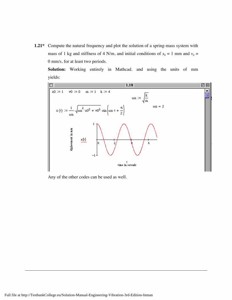
1.23 Referring to Figure 1.8, if the maximum peak velocity of a vibrating system is

200 mm/s at 4 Hz and the maximum allowable peak acceleration is 5000 mm/s2,

what will the peak displacement be?

mm/sec200=v

x (mm) a = 5000 mm/sec2

f = 4 Hz

Solution:

Given: vmax = 200 mm/s @ 4 Hz

amax = 5000 mm/s @ 4 Hz

xmax = A

vmax = Aωn

amax = Aω n 2

! xmax

=vmax

"n

=vmax

2# f=200

8#= 7.95 mm

At the center point, the peak displacement will be x = 7.95 mm



1.24 Show that lines of constant displacement and acceleration in Figure 1.8 have

slopes of +1 and –1, respectively. If rms values instead of peak values are used,

how does this affect the slope?

Solution: Let x = x

maxsin!

nt

˙ x = xmax

!n

cos!nt

˙ ̇ x = "xmax

!n

2sin!

nt

Peak values:

!xmax

= xmax!n = 2" fxmax

!!xmax

= xmax!n

2= (2" f )

2xmax

Location:

fxx

fxx

!

!

2lnlnln

2lnlnln

maxmax

maxmax

"=

+=

!!!

!

Since xmax is constant, the plot of ln maxx! versus ln 2πf is a straight line of slope

+1. If ln maxx!! is constant, the plot of ln maxx! versus ln 2πf is a straight line of

slope –1. Calculate RMS values

Let

x t( ) = Asin!

nt

˙ x t( ) = A!n

cos!nt

˙ ̇ x t( ) = "A!n

2sin!

nt



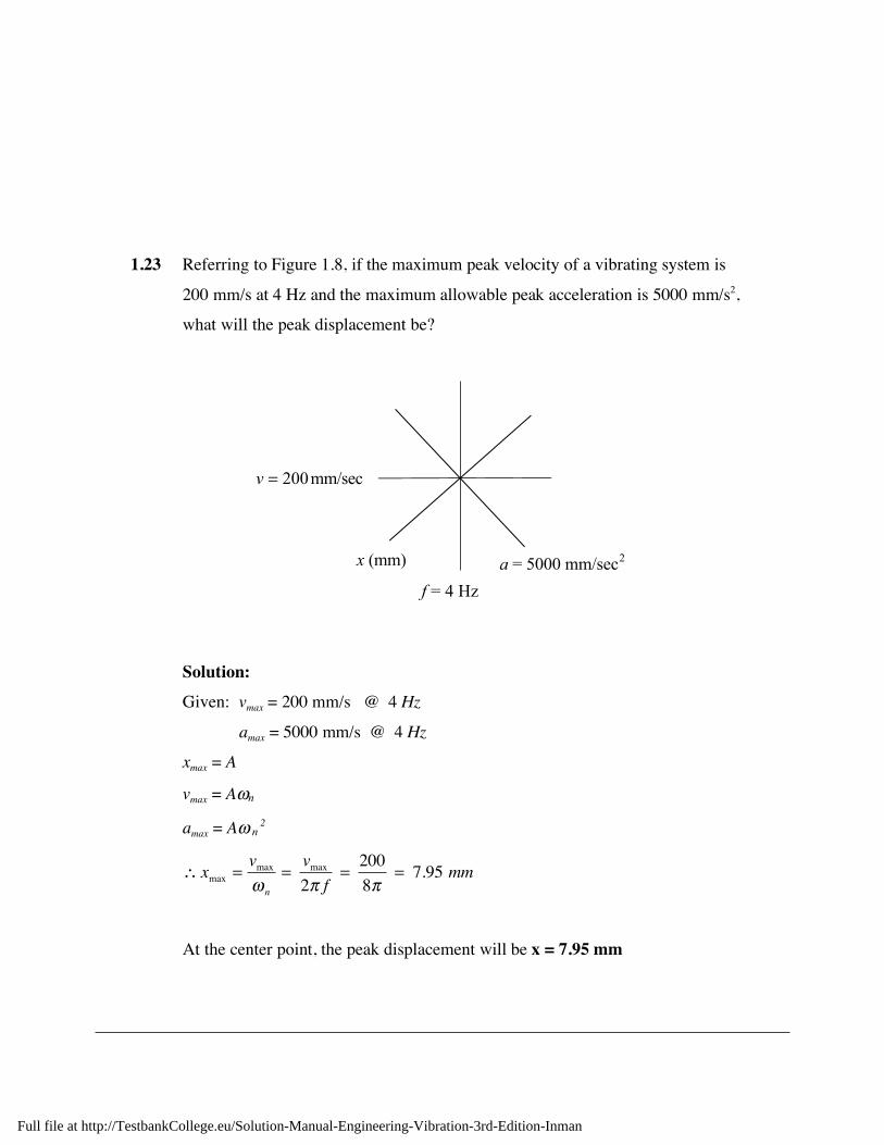
Mean Square Value: x 2 =T!"lim

1

Tx2

0

T

# (t) dt

x2=

T!"lim

1

TA2sin

2 #nt

0

T

$ dt =T!"lim

A2

T(1 % cos 2#

nt

0

T

$ ) dt =A2

2

x

.2=

T!"lim

1

TA2#

n

2cos

2#nt

0

T

$ dt =T!"lim

A2#

n

2

T

1

2(1 + cos 2#

nt

0

T

$ ) dt =A2#

n

2

2

x

..2=

T!"lim

1

TA2#

n

4sin

2#nt

0

T

$ dt =T!"lim

A2#

n

4

T

1

2(1 + cos 2#

nt

0

T

$ ) dt =A2#

n

4

2

Therefore,

Axxrms

2

22==

x.

rms = x.2=

2

2A!

n

x

..

rms = x

..2=

2

2A!

n

2

The last two equations can be rewritten as:

rmsrmsrms xfxx !="= 2

.

rmsrmsrms xfxx.

2

..

2!="=

The logarithms are:

fxx !+= 2lnlnlnmaxmax

.

fxx !+= 2lnlnln max

.

max

..

The plots of rmsx

.

ln versus f!2ln is a straight line of slope +1 when xrms is constant, and

–1 when rmsx

..

is constant. Therefore the slopes are unchanged.



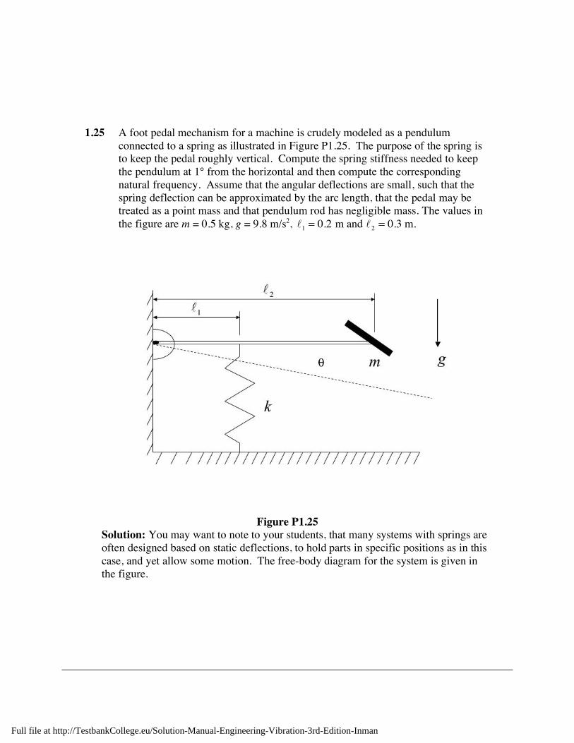
1.25 A foot pedal mechanism for a machine is crudely modeled as a pendulum connected to a spring as illustrated in Figure P1.25. The purpose of the spring is to keep the pedal roughly vertical. Compute the spring stiffness needed to keep the pendulum at 1° from the horizontal and then compute the corresponding natural frequency. Assume that the angular deflections are small, such that the spring deflection can be approximated by the arc length, that the pedal may be treated as a point mass and that pendulum rod has negligible mass. The values in the figure are m = 0.5 kg, g = 9.8 m/s2,

!

1= 0.2 m and !

2= 0.3 m.

Figure P1.25

Solution: You may want to note to your students, that many systems with springs are often designed based on static deflections, to hold parts in specific positions as in this case, and yet allow some motion. The free-body diagram for the system is given in the figure.



For static equilibrium the sum of moments about point O yields (θ1 is the static deflection):

M 0! = "!1#1(!1)k + mg!2 = 0

$ !1

2#1k = mg!2 (1)

$ k =mg!2

!1

2#1

=0.5 %0.3

(0.2)2 &

180

= 2106 N/m

Again take moments about point O to get the dynamic equation of motion:

MO! = J !!" = m"

2

2 !!" = #"1

2k(" +"

1) + mg"

2= #"

1

2k" + "

1

2k"

1# mg"

2"

Next using equation (1) above for the static deflection yields:

m!2

2 ""! + !1

2k! = 0

" ""! +!

1

2k

m!2

2

#

$%&

'(! = 0

")n=!

1

!2

k

m=

0.2

0.3

2106

0.5= 43.27 rad/s

1.26 An automobile is modeled as a 1000-kg mass supported by a spring of

stiffness k = 400,000 N/m. When it oscillates it does so with a maximum

deflection of 10 cm. When loaded with passengers, the mass increases to as much

as 1300 kg. Calculate the change in frequency, velocity amplitude, and

acceleration amplitude if the maximum deflection remains 10 cm.

Solution:

Given: m1 = 1000 kg

m2 = 1300 kg

k = 400,000 N/m



xmax = A = 10 cm

v1 = Aωn1 = 10 cm x 20 rad/s = 200 cm/s

v2 = Aωn2 = 10 cm x 17.54 rad/s = 175.4 cm/s

Δv = 175.4 - 200 = -24.6 cm/s

a1 = Aωn12 = 10 cm x (20 rad/s)2 = 4000 cm/s2

a2 = Aωn22 = 10 cm x (17.54 rad/s)2 = 3077 cm/s2

Δa = 3077 - 4000 = -923 cm/s2

sradm

k

n/20

1000

000,400

1

1 ===!

sradm

k

n/54.17

1300

000,400

2

2 ===!

srad /46.22054.17 !=!="#

!f =!"

2#=

$2.46

2#= 0.392 Hz



1.27 The front suspension of some cars contains a torsion rod as illustrated in Figure P1.27 to improve the car’s handling. (a) Compute the frequency of vibration of the wheel assembly given that the torsional stiffness is 2000 N m/rad and the wheel assembly has a mass of 38 kg. Take the distance x = 0.26 m. (b) Sometimes owners put different wheels and tires on a car to enhance the appearance or performance. Suppose a thinner tire is put on with a larger wheel raising the mass to 45 kg. What effect does this have on the frequency?

Figure P1.27

Solution: (a) Ignoring the moment of inertial of the rod, and computing the

moment of inertia of the wheel as mx2 , the frequency of the shaft mass system is

!n=

k

mx2=

2000 N "m

38 "kg (0.26 m)2= 27.9 rad/s

(b) The same calculation with 45 kg will reduce the frequency to

!n=

k

mx2=

2000 N "m

45 "kg (0.26 m)2= 25.6 rad/s

This corresponds to about an 8% change in unsprung frequency and could influence wheel hop etc. You could also ask students to examine the effect of increasing x, as commonly done on some trucks to extend the wheels out for appearance sake.



1.28 A machine oscillates in simple harmonic motion and appears to be well modeled

by an undamped single-degree-of-freedom oscillation. Its acceleration is

measured to have an amplitude of 10,000 mm/s2 at 8 Hz. What is the machine's

maximum displacement?

Solution:

Given: amax = 10,000 mm/s2 @ 8 Hz

The equations of motion for position and acceleration are:

x = Asin(!nt + ") (1.3)

!!x = #A!n

2sin(!

nt + ") (1.5)

The amplitude of acceleration is 000,102=nA! mm/s2 and ωn = 2πf = 2π(8) =

16π rad/s, from equation (1.12).

The machine's displacement is ( )2216

000,10000,10

!"

==

n

A

A = 3.96 mm

1.29 A simple undamped spring-mass system is set into motion from rest by giving it

an initial velocity of 100 mm/s. It oscillates with a maximum amplitude of 10

mm. What is its natural frequency?

Solution:

Given: x0 = 0, v0 = 100 mm/s, A = 10 mm

From equation (1.9), n

vA

!

0= or

10

1000==

A

v

n! , so that: ωn= 10 rad/s



1.30 An automobile exhibits a vertical oscillating displacement of maximum amplitude

5 cm and a measured maximum acceleration of 2000 cm/s2. Assuming that the

automobile can be modeled as a single-degree-of-freedom system in the vertical

direction, calculate the natural frequency of the automobile.

Solution:

Given: A = 5 cm. From equation (1.15)

cm/s 20002== nAx !!!

Solving for ωn yields:

!n=

2000

A=

2000

5

!n= 20rad/s



Problems Section 1.3 (Numbers 1.31 through 1.46) 1.31 Solve 04 =++ xxx !!! for x0 = 1 mm, v0 = 0 mm/s. Sketch your results and

determine which root dominates.

Solution:

Given 0 mm, 1 where04 00 ===++ vxxxx !!! Let

Substitute these into the equation of motion to get: ar

2ert+ 4are

rt+ ae

rt= 0

! r2+ 4r +1 = 0! r

1,2= "2 ± 3

So

x = a

1e

!2 + 3( ) t

+ a2e

!2 ! 3( ) t

˙ x = ! 2 + 3( )a1e

!2+ 3( ) t

+ ! 2 ! 3( )a2e

!2! 3( ) t

Applying initial conditions yields,

Substitute equation (1) into (2)

Solve for a2

Substituting the value of a2 into equation (1), and solving for a1 yields,

! x(t) =v0+ 2 + 3( )x0

2 3e

"2+ 3( ) t+

"v0+ " 2 + 3( )x0

2 3e

"2" 3( ) t

The response is dominated by the root: !2 + 3 as the other root dies off very fast.

x0 = a1 + a2 ! x0 " a2 = a1 (1)

v0 = " 2 + 3( ) a1 + " 2 " 3( )a2 (2)

v0= ! 2 + 3( )(x0 ! a2 ) + ! 2 ! 3( )a2

v0= ! 2 + 3( )x0 ! 2 3 a

2

a2=!v

0+ ! 2 + 3( ) x0

2 3

a1=v0+ 2 + 3( ) x0

2 3

x = aert! !x = are

rt! !!x = ar

2ert



1.32 Solve 022 =++ xxx !!! for x0 = 0 mm, v0 = 1 mm/s and sketch the response. You

may wish to sketch x(t) = e-t and x(t) =-e-t first.

Solution: Given 02 =++ xxx !!! where x0 = 0, v0 = 1 mm/s

Let: x = aert! !x = are

rt! !!x = ar

2ert

Substitute into the equation of motion to get

ar2ert+ 2are

rt+ ae

rt= 0! r

2+ 2r +1 = 0! r

1,2= "1± i

So

x = c

1e

!1+ i( ) t+ c

2e

!1! i( ) t" !x = !1+ i( )c

1e

!1+ i( ) t+ !1! i( )c

2e

!1! i( ) t

Initial conditions:

Substituting equation (1) into (2)

Applying Euler’s formula

Alternately use equations (1.36) and (1.38). The plot is similar to figure 1.11.

x0= x 0( ) = c

1+ c

2= 0 ! c

2= "c

1(1)

v0= ˙ x 0( ) = "1+ i( )c

1+ "1" i( )c

2=1 (2)

v0= !1 + i( )c1 ! !1! i( )c1 = 1

c1= !

1

2i, c

2=1

2i

x t( ) = !1

2ie

!1+i( ) t+1

2ie

!1! i( ) t= !

1

2ie

! t

eit

! e!it( )

x t( ) = !1

2ie

!t

cos t + isin t ! (cos t ! i sin t)( )

x t( ) = e! t sin t



1.33 Derive the form of λ1 and λ2 given by equation (1.31) from equation (1.28) and the definition of the damping ratio.

Solution:

Equation (1.28): kmcmm

c4

2

1

2

22,1 !±!="

Rewrite, !1,2

= "c

2 m m

#$%

&'(

k

k

#

$%&

'(±

1

2 m m

k

k

#

$%&

'(c

c

#$%

&'(

c2 " 2 km

2

( ) c

c

#$%

&'(2

Rearrange,!1,2

= "c

2 km

#$%

&'(

k

m

#

$%&

'(±

c

2 km

k

m

#

$%&

'(1

c

#$%

&'(

c21"

2 km

c

#

$%&

'(

2)

*++

,

-..

Substitute:

!n=

k

m and " =

c

2 km#$

1,2= %"!

n±"!

n

1

c

&'(

)*+c 1%

1

" 2

&'(

)*+

#$1,2

= %"!n±!

n" 2

1%1

" 2

&'(

)*+

,

-.

/

01

#$1,2= %"!

n±!

n" 2 %1



1.34 Use the Euler formulas to derive equation (1.36) from equation (1.35) and to

determine the relationships listed in Window 1.4.

Solution:

Equation (1.35): x t( ) = e!"# nt a1e( )

j# n 1!"2t

! a2e! j# n 1!"

2t

From Euler,

x t( ) = e!"# nt(a1 cos #n 1 !" 2 t( ) + a1 j sin #n 1 !" 2 t( )

+ a2 cos #n 1 !" 2t( ) ! a2 j sin #n 1 !" 2

t( ))= e

!"# nt a1 + a2( )cos#d t + j a1 ! a2( )sin#d t

Let: A1=( )21aa + , A2=( )

21aa ! , then this last expression becomes

x t( ) = e!"# ntA1cos#

dt + A

2sin#

dt

Next use the trig identity:

2

11

21tan,

A

AAAA

!="+=

to get: x t( ) = e!"#nt Asin(#dt + $)



1.35 Using equation (1.35) as the form of the solution of the underdamped

system, calculate the values for the constants a1 and a2 in terms of the initial

conditions x0 and v0.

Solution:

Equation (1.35):

x t( ) = e!"# nt a1ej# n 1!"

2t+ a

2e! j# n 1!"

2t( )

˙ x t( ) = (!"#n + j#n 1! "2)a1e

!"#n + j#n 1!" 2( )t+ (!"#n ! j# n 1 !" 2

)a2 e!"# n ! j#n 1!" 2( )t

Initial conditions

x0= x(0 ) = a

1+ a

2! a

1= x

0" a

2 (1)

v0= ˙ x (0) = (!"# n + j#n 1 !" 2

)a1+ (!"#n ! j#n 1 !" 2

)a2 (2)

Substitute equation (1) into equation (2) and solve for a2

v0= !"#n + j# n 1!" 2( )(x0 ! a

2) + !"#n ! j# n 1!" 2( )a2

v0= !"#n + j# n 1!" 2( )x0 ! 2 j# n 1! " 2 a

2

Solve for a2

a2=!v

0!"#

nx0+ j#

n1!" 2 x

0

2 j#n1!" 2

Substitute the value for a2 into equation (1), and solve for a1

a1=v0+ !"

nx0+ j"

n1#! 2 x

0

2 j"n1#! 2



1.36 Calculate the constants A and φ in terms of the initial conditions and thus

verify equation (1.38) for the underdamped case.

Solution:

From Equation (1.36),

x(t) = Ae!"#

ntsin #

dt + $( )

Applying initial conditions (t = 0) yields,

!= sin0

Ax (1)

!"+!#"$== cossin00

AAxvdn

! (2)

Next solve these two simultaneous equations for the two unknowns A and φ.

From (1),

!sin

0x

A = (3)

Substituting (3) into (1) yields

!

"+#"$=tan

0

00

xxv

d

n ! tan! =

x0"d

v0+#"

nx0

.

Hence,

! = tan"1 x

0#

d

v0+$#

nx0

%

&'

(

)* (4)

From (3), A

x0

sin =! (5)

and From (4), cos! =v0+"#

nx0

x0#

d( )2

+ v0+"#

nx0( )2

(6)

Substituting (5) and (6) into (2) yields,

2

2

0

2

00 )()(

d

dnxxv

A!

!"! ++=

which are the same as equation (1.38)



1.37 Calculate the constants a1 and a2 in terms of the initial conditions and thus verify

equations (1.42) and (1.43) for the overdamped case.

Solution: From Equation (1.41)

x t( ) = e!"# nt

a1e#n "

2!1 t

+ a2e!# n "

2!1 t( )

taking the time derivative yields:

˙ x t( ) = (!"#n+#

n" 2

!1)a1e!"#

n+#

n" 2

!1( )t+ (!"#

n!#

n"2

!1)a2 e!"#

n!#

n" 2

!1( )t

Applying initial conditions yields,

x0= x 0( ) = a1

+ a2

! x0" a

2= a

1 (1)

v0= !x 0( ) = "#$

n+$

n# 2 " 1( )a1

+ "#$n"$

n# 2 " 1( )a2

(2)

Substitute equation (1) into equation (2) and solve for a2

v0= !"#

n+#

n" 2 !1( )(x0 ! a2 ) + ! "#

n!#

n" 2 !1( )a2

v0= !"#

n+#

n" 2

!1( ) x0 ! 2#n" 2

!1 a2

Solve for a2

a2=!v

0!"#

nx0+#

n" 2 !1 x

0

2#n" 2 !1

Substitute the value for a2 into equation (1), and solve for a1

a1=v0+!"

nx0+"

n! 2 #1 x

0

2"n

! 2 #1



1.38 Calculate the constants a1 and a2 in terms of the initial conditions and thus verify

equation (1.46) for the critically damped case.

Solution:

From Equation (1.45),

x(t) = (a1+ a

2t)e

!"nt

! !x

0= "#

na1e"#

nt" #

na2te

"#nt+ a

2e"#

nt

Applying the initial conditions yields:

10ax = (1)

and

120 )0( aaxvn

!"== ! (2)

solving these two simultaneous equations for the two unknowns a1 and a2.

Substituting (1) into (2) yields,

01xa =

002xva

n!+=

which are the same as equation (1.46).



1.39 Using the definition of the damping ratio and the undamped natural frequency,

derive equitation (1.48) from (1.47).

Solution:

m

kn=! thus, 2

n

m

k!=

km

c

2

=! thus, n

m

km

m

c!"=

!= 22

Therefore, 0=++ xm

kx

m

cx !!!

becomes,

˙ ̇ x (t) + 2!"n

˙ x (t) +"n

2x(t ) = 0

1.40 For a damped system, m, c, and k are known to be m = 1 kg, c = 2 kg/s, k = 10

N/m. Calculate the value of ζ and ωn. Is the system overdamped, underdamped, or

critically damped?

Solution:

Given: m = 1 kg, c = 2 kg/s, k = 10 N/m

Natural frequency: sradm

kn

/16.31

10===!

Damping ratio: 316.0)1)(16.3(2

2

2==

!="

m

c

n

Damped natural frequency:

!d= 10 1"

1

10

#

$%&

'(

2

= 3.0 rad/s

Since 0 < ζ < 1, the system is underdamped.



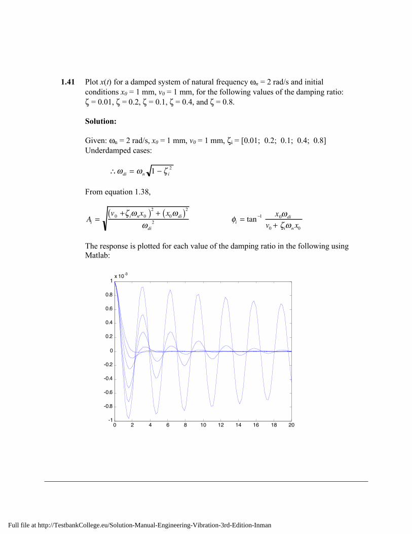
1.41 Plot x(t) for a damped system of natural frequency ωn = 2 rad/s and initial conditions x0 = 1 mm, v0 = 1 mm, for the following values of the damping ratio:

ζ = 0.01, ζ = 0.2, ζ = 0.1, ζ = 0.4, and ζ = 0.8.

Solution: Given: ωn = 2 rad/s, x0 = 1 mm, v0 = 1 mm, ζi = [0.01; 0.2; 0.1; 0.4; 0.8]

Underdamped cases: !"

di= "

n1 # $

i

2 From equation 1.38,

Ai=

v0+!

i"

nx0( )

2

+ x0"

di( )2

"di

2 !

i= tan

"1 x0#

di

v0+ $

i#

nx0

The response is plotted for each value of the damping ratio in the following using Matlab:

0 2 4 6 8 10 12 14 16 18 20

-1

-0.8

-0.6

-0.4

-0.2

0

0.2

0.4

0.6

0.8

1x 10

-3

t

x(t), mm



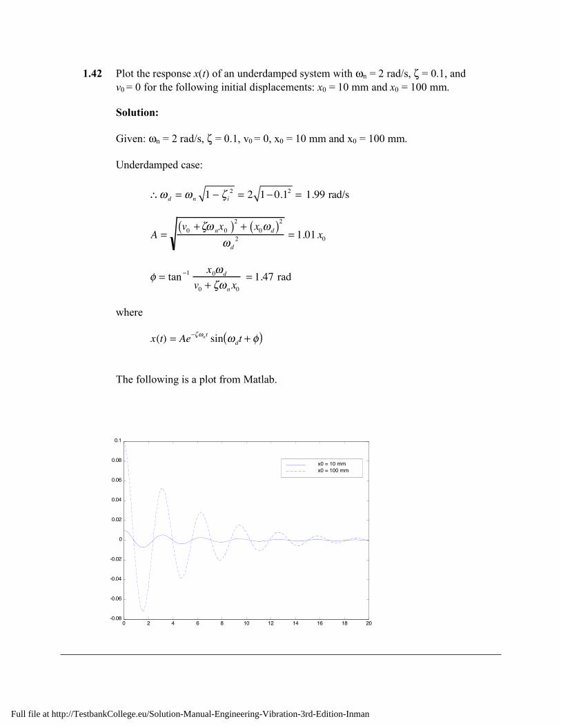
1.42 Plot the response x(t) of an underdamped system with ωn = 2 rad/s, ζ = 0.1, and v0 = 0 for the following initial displacements: x0 = 10 mm and x0 = 100 mm. Solution: Given: ωn = 2 rad/s, ζ = 0.1, v0 = 0, x0 = 10 mm and x0 = 100 mm. Underdamped case:

!"

d= "

n1 # $

i

2= 2 1#0.12 = 1.99 rad/s

A =v0+!"

nx0( )

2

+ x0"

d( )2

"d

2= 1.01 x

0

! = tan"1 x

0#

d

v0+ $#

nx0

= 1.47 rad

where x(t) = Ae

!"#ntsin #

dt + $( )

The following is a plot from Matlab.

0 2 4 6 8 10 12 14 16 18 20-0.08

-0.06

-0.04

-0.02

0

0.02

0.04

0.06

0.08

0.1

t

x(t), mm

x0 = 10 mm

x0 = 100 mm



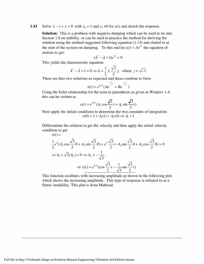
1.43 Solve 0=+! xxx !!! with x0 = 1 and v0 =0 for x(t) and sketch the response.

Solution: This is a problem with negative damping which can be used to tie into Section 1.8 on stability, or can be used to practice the method for deriving the solution using the method suggested following equation (1.13) and eluded to at the start of the section on damping. To this end let x(t) = Ae!t the equation of motion to get:

(!2" ! +1)e

!t= 0

This yields the characteristic equation:

!2" ! +1 = 0 #! =

1

2±

3

2j, where j = "1

There are thus two solutions as expected and these combine to form

x(t) = e0.5t(Ae

3

2jt

+ Be!3

2jt

) Using the Euler relationship for the term in parenthesis as given in Window 1.4, this can be written as

x(t) = e0.5t(A1 cos

3

2t + A2 sin

3

2t)

Next apply the initial conditions to determine the two constants of integration: x(0) = 1 = A

1(1) + A

2(0)! A

1=1

Differentiate the solution to get the velocity and then apply the initial velocity condition to get

!x(t) =

1

2e

0(A1 cos

3

20 + A2 sin

3

20) + e

0 3

2(!A1 sin

3

20 + A2 cos

3

20) = 0

" A1 + 3(A2 ) = 0 " A2 = !1

3,

" x(t) = e0.5t

(cos3

2t !

1

3sin

3

2t)

This function oscillates with increasing amplitude as shown in the following plot which shows the increasing amplitude. This type of response is referred to as a flutter instability. This plot is from Mathcad.



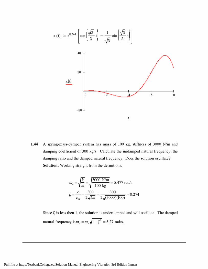
1.44 A spring-mass-damper system has mass of 100 kg, stiffness of 3000 N/m and

damping coefficient of 300 kg/s. Calculate the undamped natural frequency, the

damping ratio and the damped natural frequency. Does the solution oscillate?

Solution: Working straight from the definitions:

!n=

k

m=

3000 N/m

100 kg= 5.477 rad/s

" =c

ccr

=300

2 km=

300

2 (3000)(100)= 0.274

Since ζ is less then 1, the solution is underdamped and will oscillate. The damped

natural frequency is!d=!

n1 "#2

= 5.27 rad/s.



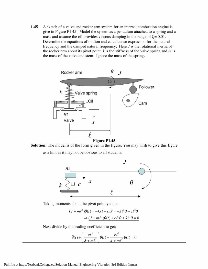
1.45 A sketch of a valve and rocker arm system for an internal combustion engine is give in Figure P1.45. Model the system as a pendulum attached to a spring and a mass and assume the oil provides viscous damping in the range of ζ = 0.01. Determine the equations of motion and calculate an expression for the natural frequency and the damped natural frequency. Here J is the rotational inertia of the rocker arm about its pivot point, k is the stiffness of the valve spring and m is the mass of the valve and stem. Ignore the mass of the spring.

Figure P1.45

Solution: The model is of the form given in the figure. You may wish to give this figure

as a hint as it may not be obvious to all students.

Taking moments about the pivot point yields:

(J + m!2)""!(t) = "kx! " c"x! = "k!

2! " c!

2 "!

# (J + m!2)""!(t) + c!

2 "! + k!2! = 0

Next divide by the leading coefficient to get;

!!!(t) +c"

2

J + m"2

"#$

%&'!!(t) +

k"2

J + m"2!(t) = 0



From the coefficient of q, the undamped natural frequency is

!n=

k!2

J + m!2

rad/s

From equation (1.37), the damped natural frequency becomes

!d=!

n1"# 2 = 0.99995

k!2

J + m!2"

k!2

J + m!2

This is effectively the same as the undamped frequency for any reasonable

accuracy. However, it is important to point out that the resulting response will

still decay, even though the frequency of oscillation is unchanged. So even

though the numerical value seems to have a negligible effect on the frequency of

oscillation, the small value of damping still makes a substantial difference in the

response.

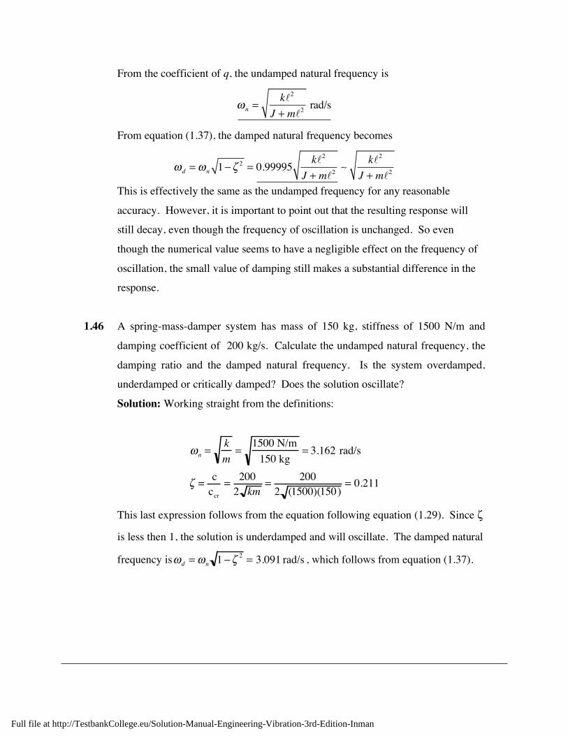
1.46 A spring-mass-damper system has mass of 150 kg, stiffness of 1500 N/m and

damping coefficient of 200 kg/s. Calculate the undamped natural frequency, the

damping ratio and the damped natural frequency. Is the system overdamped,

underdamped or critically damped? Does the solution oscillate?

Solution: Working straight from the definitions:

!n=

k

m=

1500 N/m

150 kg= 3.162 rad/s

" =c

ccr

=200

2 km=

200

2 (1500)(150)= 0.211

This last expression follows from the equation following equation (1.29). Since ζ

is less then 1, the solution is underdamped and will oscillate. The damped natural

frequency is!d=!

n1 "# 2

= 3.091 rad/s , which follows from equation (1.37).



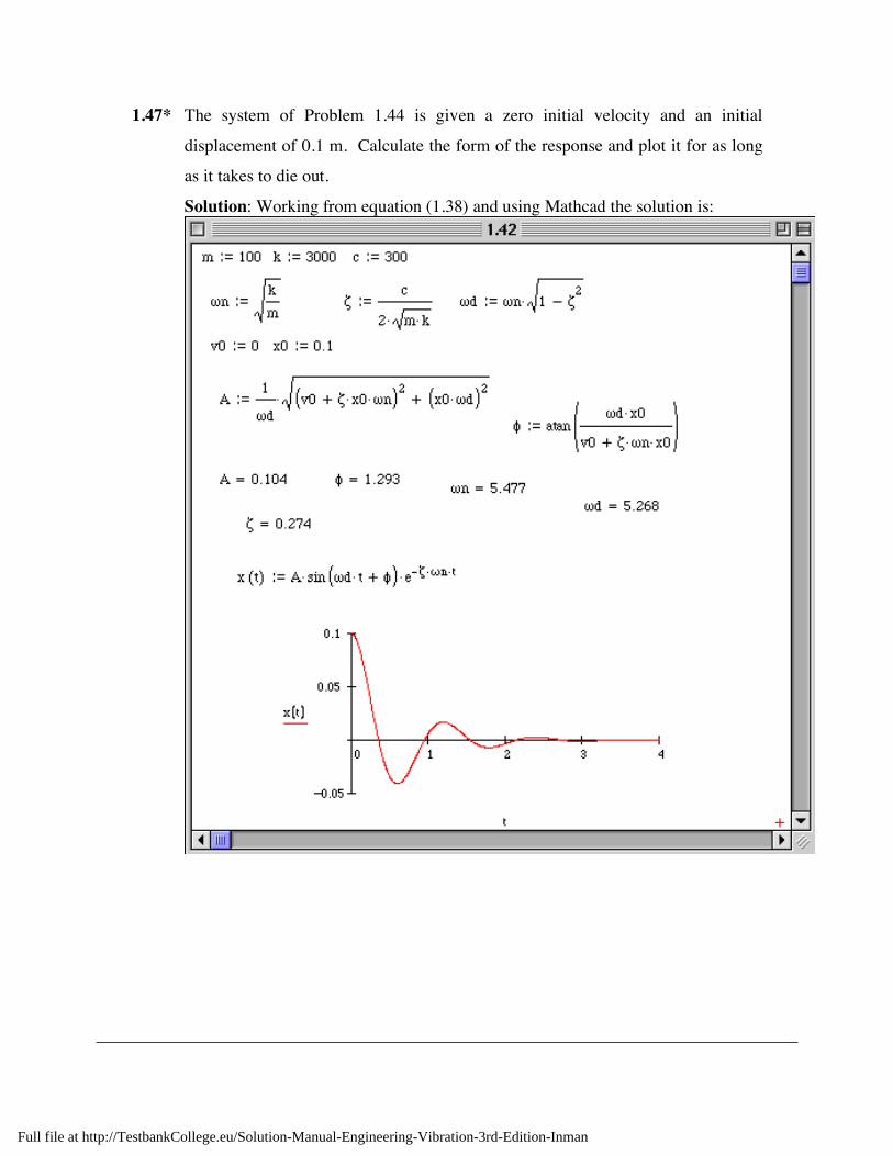
1.47* The system of Problem 1.44 is given a zero initial velocity and an initial

displacement of 0.1 m. Calculate the form of the response and plot it for as long

as it takes to die out.

Solution: Working from equation (1.38) and using Mathcad the solution is:



1.48* The system of Problem 1.46 is given an initial velocity of 10 mm/s and an initial

displacement of -5 mm. Calculate the form of the response and plot it for as long

as it takes to die out. How long does it take to die out?

Solution: Working from equation (1.38), the form of the response is programmed in Mathcad and is given by:

It appears to take a little over 6 to 8 seconds to die out. This can also be plotted in Matlab, Mathematica or by using the toolbox.



1.49* Choose the damping coefficient of a spring-mass-damper system with mass of

150 kg and stiffness of 2000 N/m such that it’s response will die out after about 2

s, given a zero initial position and an initial velocity of 10 mm/s.

Solution: Working in Mathcad, the response is plotted and the value of c is

changed until the desired decay rate is meet:

In this case ζ = 0.73 which is very large!

k 2000

x0 0v0 0.010

m 150

c 800

!nk

m

!c

.2 .m k

!d .!n 1 "2

! atan

."d x0

v0 ..# "n x0

x t ..A sin .!n t " e..# !n t

0 0.5 1 1.5 2 2.5 3

0.002

0.002

x t

t



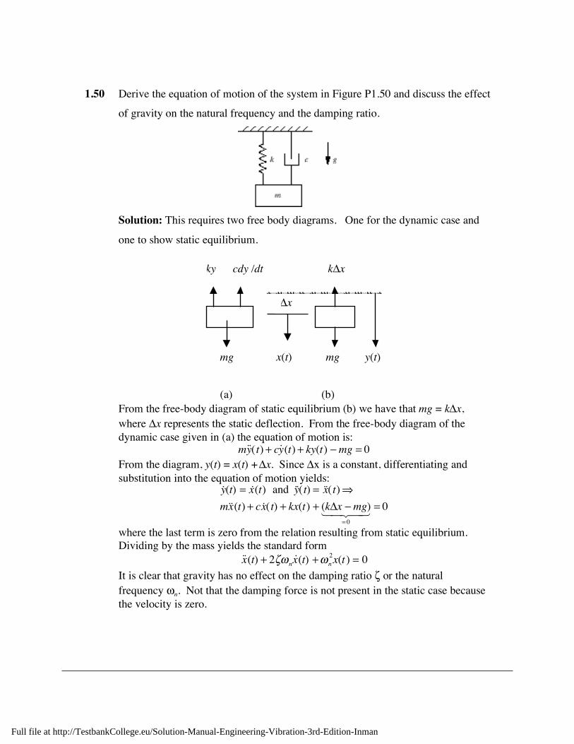
1.50 Derive the equation of motion of the system in Figure P1.50 and discuss the effect

of gravity on the natural frequency and the damping ratio.

Solution: This requires two free body diagrams. One for the dynamic case and

one to show static equilibrium.

!x

mg x(t) mg y(t)

ky cdy /dt k!x

(a) (b)

From the free-body diagram of static equilibrium (b) we have that mg = kΔx, where Δx represents the static deflection. From the free-body diagram of the dynamic case given in (a) the equation of motion is:

m˙ ̇ y ( t) + c˙ y (t) + ky(t) ! mg = 0 From the diagram, y(t) = x(t) + Δx. Since Δx is a constant, differentiating and substitution into the equation of motion yields:

˙ y (t) = ˙ x (t) and ˙ ̇ y ( t) = ˙ ̇ x ( t)!

m˙ ̇ x (t) + c ˙ x ( t) + kx(t) + (k"x # mg)

= 0

! " # $ # = 0

where the last term is zero from the relation resulting from static equilibrium. Dividing by the mass yields the standard form

˙ ̇ x (t) + 2!"n˙ x (t) +"

n

2x(t ) = 0

It is clear that gravity has no effect on the damping ratio ζ or the natural frequency ωn. Not that the damping force is not present in the static case because the velocity is zero.



1.51 Derive the equation of motion of the system in Figure P1.46 and discuss the effect

of gravity on the natural frequency and the damping ratio. You may have to make

some approximations of the cosine. Assume the bearings provide a viscous

damping force only in the vertical direction. (From the A. Diaz-Jimenez, South

African Mechanical Engineer, Vol. 26, pp. 65-69, 1976)

Solution: First consider a free-body diagram of the system:

x(t)

c ˙ x (t) k!!

Let α be the angel between the damping and stiffness force. The equation of

motion becomes

m˙ ̇ x (t) = !c˙ x (t) ! k("! +#

s)cos$

From static equilibrium, the free-body diagram (above with c = 0 and stiffness force kδs) yields: Fx = 0 =mg ! k" s cos#$ . Thus the equation of motion becomes

m˙ ̇ x + c ˙ x + k!!cos" = 0 (1) Next consider the geometry of the dynamic state:



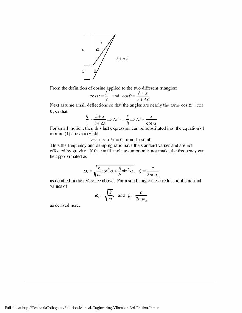
h

x !

!

"

! +# !

From the definition of cosine applied to the two different triangles:

cos! =h

! and cos" =

h + x

! + #!

Next assume small deflections so that the angles are nearly the same cos α = cos θ, so that

h

!!h + x

!+ "!# "! ! x

!

h# "! !

x

cos$

For small motion, then this last expression can be substituted into the equation of motion (1) above to yield:

m˙ ̇ x + c ˙ x + kx = 0 , α and x small Thus the frequency and damping ratio have the standard values and are not effected by gravity. If the small angle assumption is not made, the frequency can be approximated as

!n =k

mcos

2" +g

hsin

2 " , # =c

2m! n

as detailed in the reference above. For a small angle these reduce to the normal values of

!n=

k

m, and " =

c

2m!n

as derived here.



Problems and Solutions for Section 1.2 and Section 1.3...

Documents

Transcript of Problems and Solutions for Section 1.2 and Section 1.3...