Problemas Analíticos para la Ecuación de Boltzmann

Analytical issues from the Boltzmann Transport Equation

Irene M. Gamba

The University of Texas at AustinMathematics and ICES

Work in collaboration with Ricardo Alonso, Rice University

Emanuel Carneiro, IAS

UMA – Mar del Plata September 2009

• Classical problem: Rarefied ideal gases: conservativeconservative Boltzmann Transport eq.Boltzmann Transport eq.

• Energy dissipative phenomena: Gas of elastic or inelastic interacting systems in the presence of a thermostat with a fixed background temperature өb or Rapid granular flow dynamics: (inelastic hard sphere interactions): homogeneous cooling states, randomly heated states, shear flows, shockwaves past wedges, etc.

•(Soft) condensed matter at nano scale; mean field theory of charged transport: Bose-Einstein condensates models, Boltzmann Poisson charge transport in electro chemistry and materials: hot electron transport and semiconductor modeling.

•Emerging applications from stochastic dynamics and connections to probability theory for multi-linear Maxwell type interactions : Social networks, Pareto tails for wealth distribution, non-conservative dynamics: opinion dynamic and information percolation models in social dynamics, particle swarms in population dynamics, etc.

Today: The classical Boltzmann equation: Today: The classical Boltzmann equation:

•convolution estimates, exact and best constantsconvolution estimates, exact and best constants

•Existence and stability for in a certain class of initial dataExistence and stability for in a certain class of initial data and Land Lpp stability of the initial value problem stability of the initial value problem

• Spectral-Lagrangian solvers for BTESpectral-Lagrangian solvers for BTE

OverviewOverviewPart IPart I

•Introduction to classical kinetic equations for elastic and inelastic interactions: The Boltzmann equation for binary elastic and inelastic collisions * Description of interactions, collisional frequency and potentials * Energy dissipation & heat source mechanisms * * Revision of Elastic (conservative) vs inelastic (dissipative) theory.

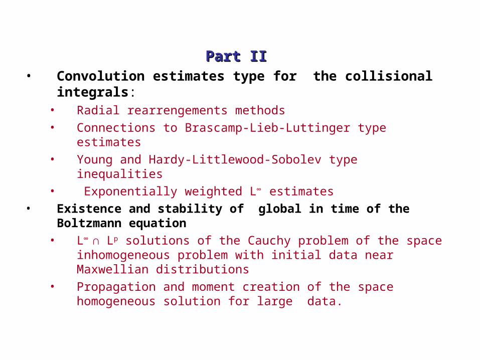
Part IIPart II• Convolution estimates type for the collisional integrals:

• Radial rearrengements methods

• Connections to Brascamp-Lieb-Luttinger type estimates

• Young and Hardy-Littlewood-Sobolev type inequalities

• Exponentially weighted L∞ estimates

• Existence and stability of global in time of the Boltzmann equation

• L∞ ∩ Lp solutions of the Cauchy problem of the space inhomogeneous problem with initial data near Maxwellian distributions

• Propagation and moment creation of the space homogeneous solution for large data.

• Dissipative models for Variable hard potentials with heating sources:

All moments bounded Stretched exponential high energy tails

Some issues of variable hard and soft potential interactionsSome issues of variable hard and soft potential interactions

Spectral - Lagrange solvers for collisional problemsSpectral - Lagrange solvers for collisional problems

• Deterministic solvers for Dissipative models - The space homogeneous problem

• FFT application - Computations of Self-similar solutions

• Space inhomogeneous problems Time splitting algorithms

Simulations of boundary value – layers problemsBenchmark simulations

Part IIIPart III

‘v

‘v*

v

v*

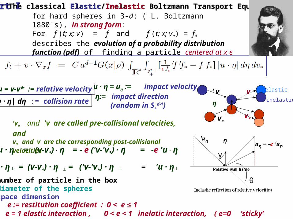
C = number of particle in the box a = diameter of the spheresd = space dimension

η

elastic

inelastic

u · η = uη := impact velocity η:= impact direction (random in S+

d-1)

u · η = (v-v*) . η = - e ('v-'v*) · η = -e 'u . η

u · η ┴ = (v-v*) · η ┴ = ('v-'v*) · η ┴ = 'u · η ┴

for hard spheres in 3-d: ( L. Boltzmann 1880's), in strong form: For f (t; x; v) = f and f (t; x; v*) = f* describes the evolution of a probability distribution function (pdf) of finding a particle centered at x ϵ d, with velocity v ϵ d, at time t ϵ + , satisfying

e := restitution coefficient : 0 < e ≤ 1e = 1 elastic interaction , 0 < e < 1 inelatic interaction, ( e=0 ‘sticky’ particles)

u = v-v* := relative velocity

|u · η| dη := collision rate

The classicalThe classical Elastic Elastic//InelasticInelastic Boltzmann Transport Equation Boltzmann Transport EquationPart IPart I

γ

θ

'v* and 'v are called pre-collisional velocities, and v* and v are the corresponding post-collisional velocities

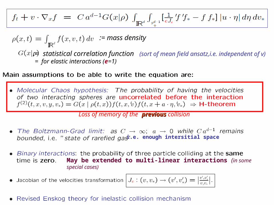
i.e. enough intersitial space

May be extended to multi-linear interactions (in some special cases)

:= statistical correlation function (sort of mean field ansatz,i.e. independent of v) = for elastic interactions (e=1)

:= mass density

Loss of memory of the previous previous collision

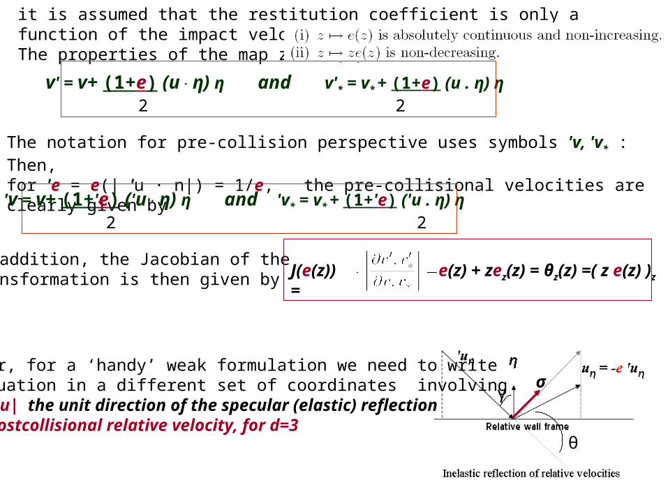
it is assumed that the restitution coefficient is only a function of the impact velocity e = e(|u·n|). The properties of the map z e(z) are

v' = v+ (1+e) (u . η) η and v'* = v* + (1+e) (u . η) η 2 2

The notation for pre-collision perspective uses symbols 'v, 'v* : Then, for 'e = e(| 'u · n|) = 1/e, the pre-collisional velocities are clearly given by

'v = v+ (1+'e) ('u . η) η and 'v* = v* + (1+'e) ('u . η) η 2 2

e(z) + zez(z) = θz(z) =( z e(z) )zJ(e(z)) =In addition, the Jacobian of the transformation is then given by

γ

θ

However, for a ‘handy’ weak formulation we need to write the equation in a different set of coordinates involvingσ := u'/|u| the unit direction of the specular (elastic) reflectionof the postcollisional relative velocity, for d=3

σ

v*

v

.σ

u

v'*

v'

u'

η

θ

v*

v

.σ

..

1-β

u

v'*

v'

β

u'

e

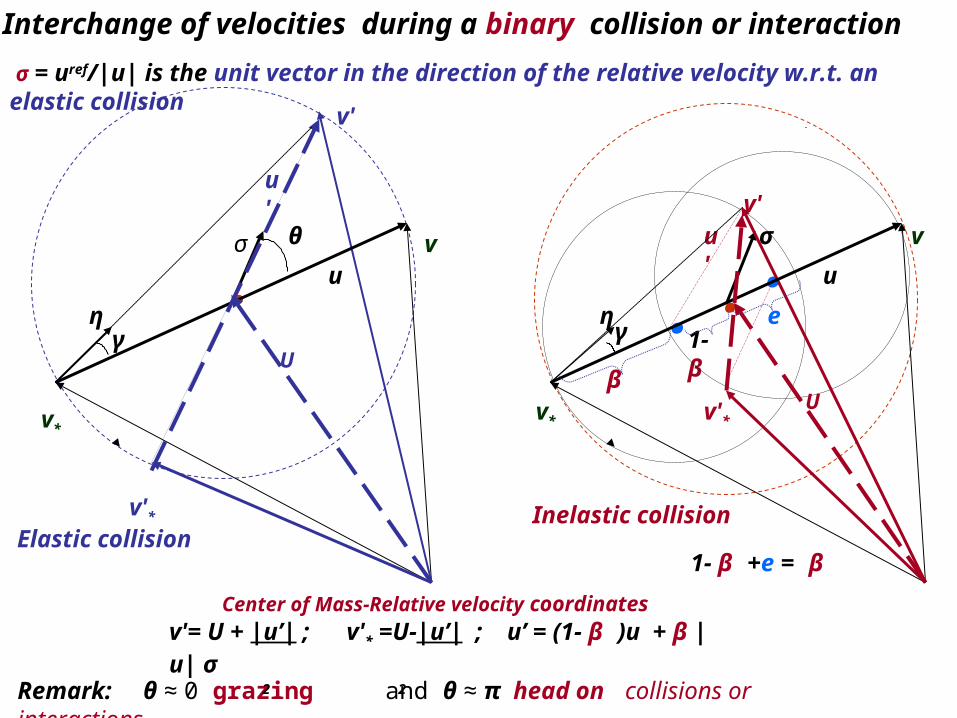
1- β +e = β

η

Elastic collisionInelastic collision

σ = uref/|u| is the unit vector in the direction of the relative velocity w.r.t. an elastic collision

Interchange of velocities during a binary collision or interaction

γ γ

Remark: θ ≈ 0 grazing and θ ≈ π head on collisions or interactions

U

U

Center of Mass-Relative velocity coordinates v'= U + |u’| ; v'* =U-|u’| ; u’ = (1- β )u + β |u| σ 2 2

σ

Goal: Write the BTE in ( (v +v*)/2 ; u) = (center of mass, relative velocity) coordinates.Let u = v – v* the relative velocity associated to an elastic interaction. Let P be the orthogonal plane to u. Spherical coordinates to represent the d-space spanned by {u; P} are {r; φ; ε1; ε2;…; εd-2}, where r = radialcoordinates, φ = polar angle, and{ε1; ε2;…; εd-2}, the n-2 azimuthal angular variables.

then with , θ = scattering angle

• 0 ≤ sin γ = b/a ≤ 1, with b = impact parameter, a = diameter of particle

• Assume scattering effects are symmetric with respect to θ = 0 → 0 ≤ θ ≤ π ↔ 0 ≤ γ ≤ π/2

• The unit direction σ is the specular reflection of u w.r.t. γ, that is |u|σ = u-2(u · η) η

• Then write the BTE collisional integral with the σ-direction dη dv* → dσ dv* , η, σ in Sd-1

using the identity

b(|u · σ| )dσ = |Sd-2| ∫0 b(z) (1-z2) (d-3)/2 dz

|u|

1

∫ Sd-1

In addition, since then any function b(u · σ) defined on Sd-1 satisfies

|u|

dσ = |Sd-2| sind-2 θ dθ ,

, z=cosθ

So the exchange of coordinates can be performed.

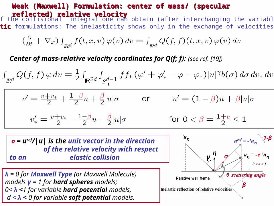
Weak (Maxwell) Formulation: center of mass/ (specular reflected) relative velocity Weak (Maxwell) Formulation: center of mass/ (specular reflected) relative velocity

Due to symmetries of the collisional integral one can obtain (after interchanging the variables of integration) Both Elastic/Elastic/inelasticinelastic formulations: The inelasticity shows only in the exchange of velocities.

Center of mass-relative velocity coordinates for Q(f; f): (see ref. [19])

β

σ = uref/|u| is the unit vector in the direction of the relative velocity with respect to an elastic collision

1-β

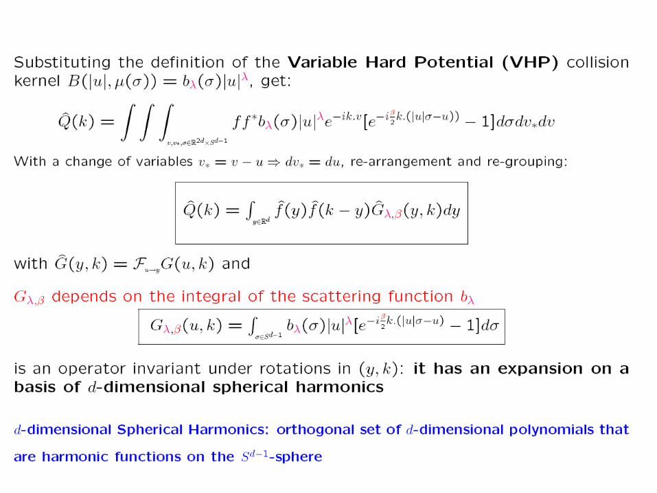
λ = 0 for Maxwell Type (or Maxwell Molecule) models γ = 1 for hard spheres models; 0< λ <1 for variable hard potential models,-d < λ < 0 for variable soft potential models.

γ

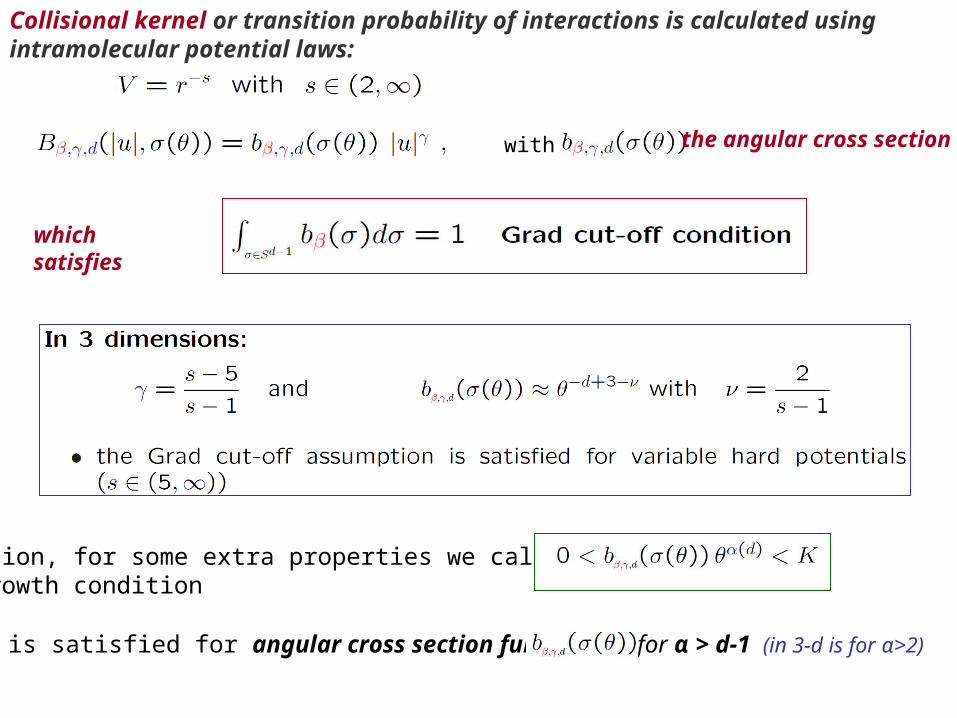
In addition, for some extra properties we call for the α-growth condition

which is satisfied for angular cross section function for α > d-1 (in 3-d is for α>2)

the angular cross section

which satisfies

Collisional kernel or transition probability of interactions is calculated using intramolecular potential laws:

with

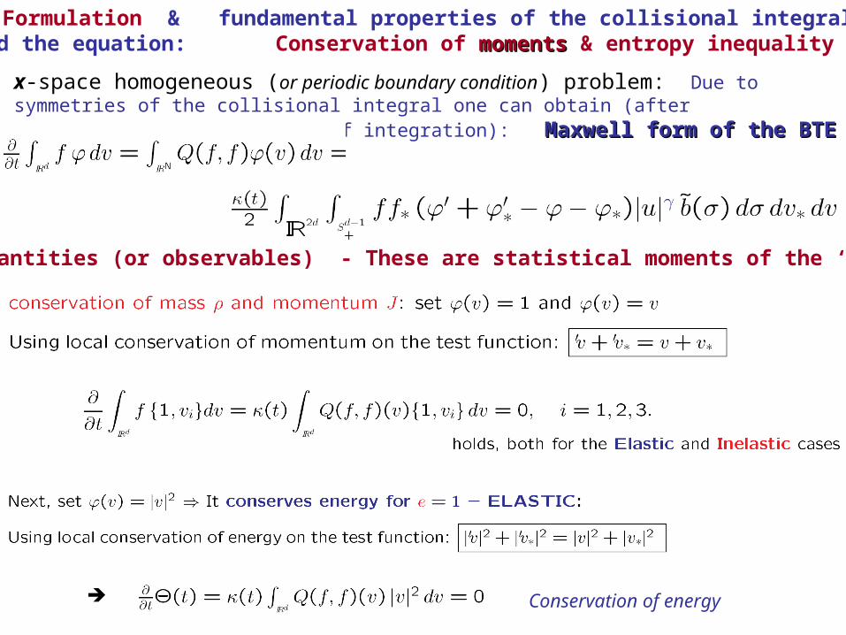
Weak Formulation & fundamental properties of the collisional integral and the equation: Conservation of momentsmoments & entropy inequality

x-space homogeneous (or periodic boundary condition) problem: Due to symmetries of the collisional integral one can obtain (after interchanging the variables of integration): Maxwell form of the BTEMaxwell form of the BTE

Invariant quantities (or observables) - These are statistical moments of the ‘pdf’

Conservation of energy

The Boltzmann Theorem:The Boltzmann Theorem: there are only N+2 collision invariants

Time irreversibility is expressed in this inequality stability

In addition:

→ yields the compressible Euler equations

Elastic (conservative) InteractionsElastic (conservative) Interactions

Hydrodynamic limits: evolution models of a ‘few’ statistical momentsHydrodynamic limits: evolution models of a ‘few’ statistical moments (mass, momentum and energy) (mass, momentum and energy)

Elastic (conservative) Interactions: Elastic (conservative) Interactions: Connections to Connections to

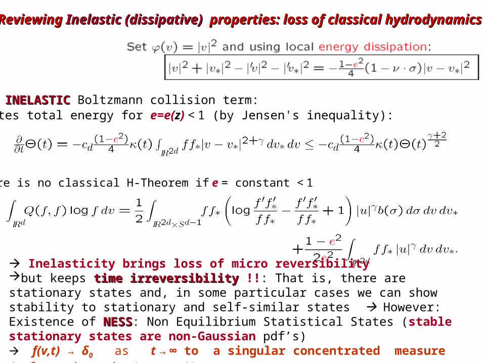
Reviewing Reviewing Inelastic (dissipative) Inelastic (dissipative) properties: loss of classical hydrodynamicsproperties: loss of classical hydrodynamics

INELASTICINELASTIC Boltzmann collision term:

Inelasticity brings loss of micro reversibilitybut keeps time irreversibilitytime irreversibility !!: That is, there are stationary states and, in some particular cases we can show stability to stationary and self-similar states However: Existence of NESSNESS: Non Equilibrium Statistical States (stable stationary states are non-Gaussian pdf’s) f(v,t) → δ0 as t → ∞ to a singular concentrated measure (unless there is ‘source’)(Multi-linear Maxwell molecule equations of collisional type and variable hard potentials for collisions with a background thermostat)

It dissipates total energy for e=e(z) < 1 (by Jensen's inequality):

and there is no classical H-Theorem if e = constant < 1

Part IIPart II• Convolution estimates type for the collisional integrals:

• Radial rearrengements methods

• Connections to Brascamp-Lieb-Luttinger type estimates

• Young and Hardy-Littlewood-Sobolev type inequalities

• Exponentially weighted L∞ estimates

• Existence and stability of global in time of the Boltzmann equation

• L∞ ∩ Lp solutions of the Cauchy problem of the space inhomogeneous problem with initial data near Maxwellian distributions

• Propagation and moment creation of the space homogeneous solution for large data.

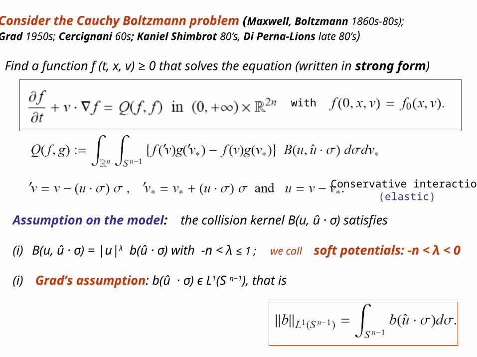
Consider the Cauchy Boltzmann problem (Maxwell, Boltzmann 1860s-80s);

Grad 1950s; Cercignani 60s; Kaniel Shimbrot 80’s, Di Perna-Lions late 80’s) Find a function f (t, x, v) ≥ 0 that solves the equation (written in strong form)

Assumption on the model: the collision kernel B(u, û · σ) satisfies

(i) B(u, û · σ) = |u|λ b(û · σ) with -n < λ ≤ 1 ; we call soft potentials: -n < λ < 0

(i) Grad’s assumption: b(û · σ) є L1(S n−1), that is

with

Conservative interaction(elastic)

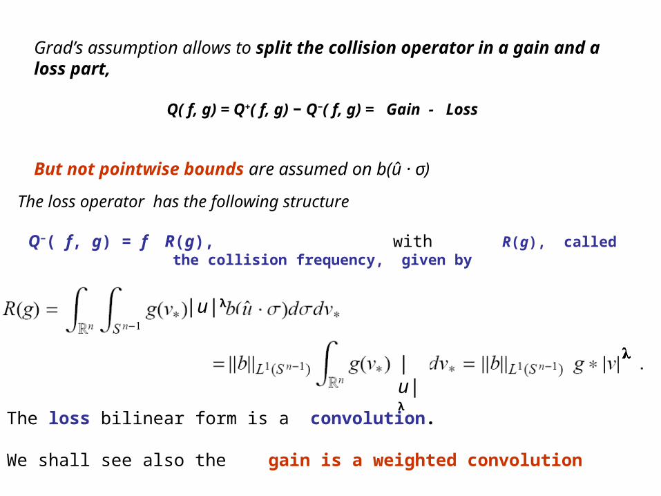
Grad’s assumption allows to split the collision operator in a gain and a loss part,

Q( f, g) = Q+( f, g) − Q−( f, g) = Gain - Loss

But not pointwise bounds are assumed on b(û · σ)

The loss operator has the following structure

Q−( f, g) = f R(g), with R(g), called the collision frequency, given by

The loss bilinear form is a convolution.

We shall see also the gain is a weighted convolution

|u|λ

|u|λ

Exchange of velocities in center of mass-relative velocity frame

Energy dissipation parameter or restitution parameters

Recall: Q+(v) operator in weak (Maxwell) form, and then it can easily be extended to dissipative (inelastic) collisions

Same the collision kernel form

With the Grad Cut-off assumption:

with

Q−( f, g) = fAnd convolution structure in the loss term: λ

Outline of recent work

Average angular estimates (for the inelastic case as well) by means of radial rearrengement Average angular estimates (for the inelastic case as well) by means of radial rearrengement argumentsarguments• Young’s inequalities for 1 ≤ p , q , r ≤ ∞ Young’s inequalities for 1 ≤ p , q , r ≤ ∞ (with exact constants) (with exact constants) for Maxwell type and hard for Maxwell type and hard potentials |u|potentials |u|λλ with with 0 0 ≤≤ λλ = 1 = 1

Sharp constantsSharp constants for for Maxwell typeMaxwell type interaction for (p, q , r) = interaction for (p, q , r) = (1,2, 2) and (2,1,2) λλ = 0= 0 • Hardy Littlewood Sobolev inequalities , for 1 < p , q , r < ∞ Hardy Littlewood Sobolev inequalities , for 1 < p , q , r < ∞ (with exact constants) (with exact constants) for soft for soft potentialspotentials |u||u|λλ withwith -n -n ≤≤ λλ < 0 < 0

• Triple Young’s inequalities for 1 ≤ p , q , r, s ≤ ∞ Triple Young’s inequalities for 1 ≤ p , q , r, s ≤ ∞ (with exact constants) (with exact constants) for radial non-for radial non-increasing potentials in Lincreasing potentials in Ls(R(Rdd))

•Existence, uniqueness and regularity estimates for the near vacuum and near (different) Existence, uniqueness and regularity estimates for the near vacuum and near (different) Maxwellian solutions for the space inhomogeneous problem (using Kaniel-Shimbrot iteration Maxwellian solutions for the space inhomogeneous problem (using Kaniel-Shimbrot iteration type solutions) elastic interactions for soft potential and the above estimates.type solutions) elastic interactions for soft potential and the above estimates.

• LLpp stability estimates in the soft potential case, for 1 stability estimates in the soft potential case, for 1 ≤≤ p p ≤≤ ∞ ∞

Work in n collaboration with Ricardo Alonso and Emanuel Carneiro

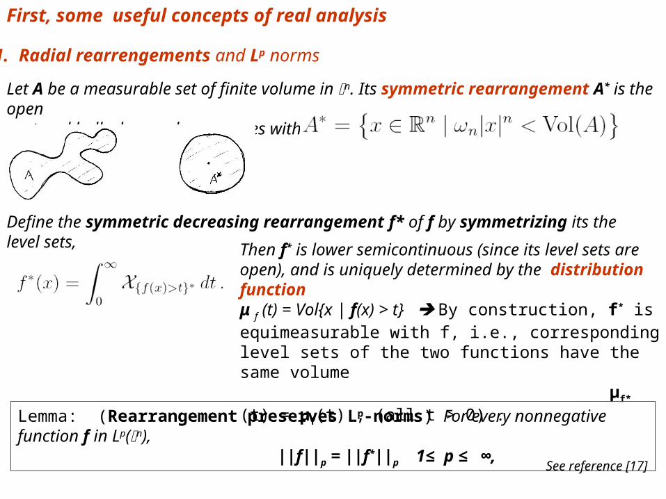
Let A be a measurable set of finite volume in n. Its symmetric rearrangement A* is the opencentered ball whose volume agrees with A:

Define the symmetric decreasing rearrangement f* of f by symmetrizing its the level sets,

Then f* is lower semicontinuous (since its level sets are open), and is uniquely determined by the distribution function μ f (t) = Vol{x | f(x) > t} By construction, f* is equimeasurable with f, i.e., corresponding level sets of the two functions have the same volume μf* (t) = μf(t) , (all t > 0) .

Lemma: (Rearrangement preserves Lp-norms) For every nonnegative function f in Lp(n), ||f||p = ||f*||p 1≤ p ≤ ∞,

First, some useful concepts of real analysis

See reference [17]

1. Radial rearrengements and Lp norms

2. Brascamp, Lieb, and Luttinger (1974) showed that functionals of the form

can only increase under a radial rearrangement, where the ηij form an arbitrary real n×m matrix. Moreover, they obtain exact inequality constants

3. Beckner (75), Brascamp-Lieb (76, 83) calculation of best/sharp constants for maximizations by radial rearrangements by constructing a family of optimizers.

1. Calculation of Young and Hardy-Littlewood-Sobolev (convolutions) inequalities with exact and best constants – Also extended to multiple Young’s ineq.

1. Applications to problems in mathematical physics where the solutions are probabilities, i.e. Ornstein-Uhlenbeck; Fokker Plank equations, optimal decay rates to equilibrium, stability estimatesIsoperimetric inequalities, etc.

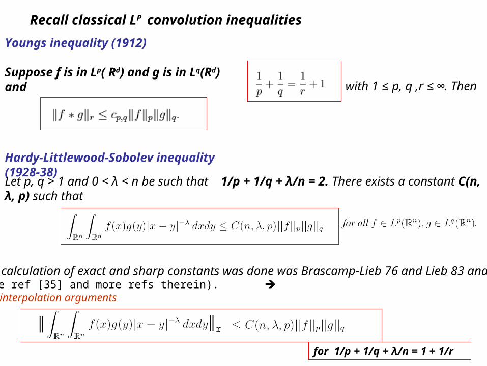
Hardy-Littlewood-Sobolev inequality (1928-38)

Recall classical LP convolution inequalities

Suppose f is in Lp( Rd) and g is in Lq(Rd) and with 1 ≤ p, q ,r ≤ ∞. Then

Youngs inequality (1912)

Let p, q > 1 and 0 < λ < n be such that 1/p + 1/q + λ/n = 2. There exists a constant C(n, λ, p) such that

The calculation of exact and sharp constants was done was Brascamp-Lieb 76 and Lieb 83 and 90(see ref [35] and more refs therein). By interpolation arguments

║ ║r

for 1/p + 1/q + λ/n = 1 + 1/r

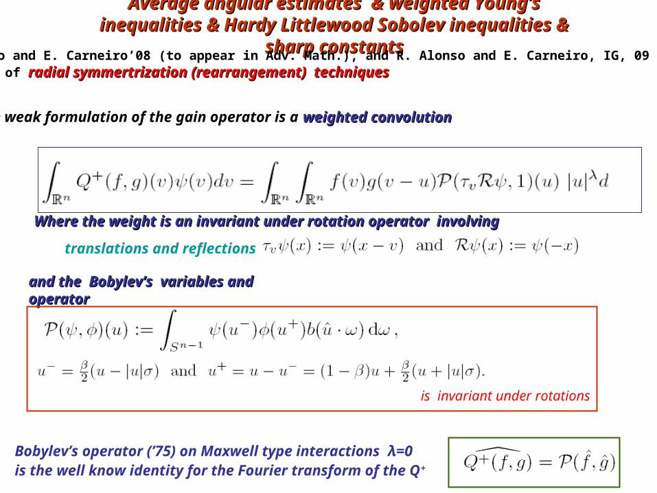
Average angular estimates & weighted Young’s inequalities & Average angular estimates & weighted Young’s inequalities & Hardy Littlewood Sobolev inequalities & sharp constantsHardy Littlewood Sobolev inequalities & sharp constants

R. Alonso and E. Carneiro’08 (to appear in Adv. Math.), and R. Alonso and E. Carneiro, IG, 09 (refs[1,2]):by means of radial symmertrization (rearrangement) techniques radial symmertrization (rearrangement) techniques

and the Bobylev’s variables and operatorand the Bobylev’s variables and operator

Bobylev’s operator (’75) on Maxwell type interactions λ=0is the well know identity for the Fourier transform of the Q+

translations and reflections

is invariant under rotations

The weak formulation of the gain operator is a weighted convolutionweighted convolution

Where the weight is an invariant under rotation operator involving Where the weight is an invariant under rotation operator involving

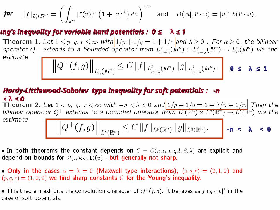
Young’s inequality for variable hard potentials : 0 Young’s inequality for variable hard potentials : 0 ≤≤ λ ≤≤ 1 1

Hardy-Littlewood-Sobolev type inequality for soft potentials Hardy-Littlewood-Sobolev type inequality for soft potentials : : -n -n << λ << 00

for

0 ≤0 ≤ λλ ≤ 1 ≤ 1

-n <-n < λλ < 0 < 0

Sketch of proof: important facts

1- Radial rearrangement

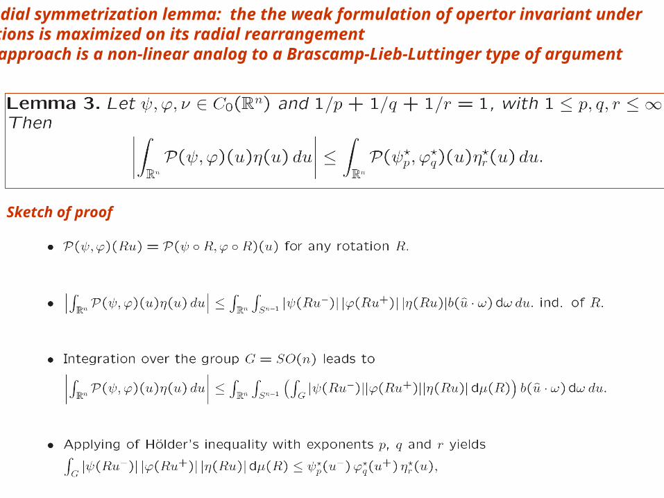
2- Radial symmetrization lemma: the the weak formulation of opertor invariant under rotations is maximized on its radial rearrangement This approach is a non-linear analog to a Brascamp-Lieb-Luttinger type of argument

Sketch of proof

and for set

α corresponds to moments weights

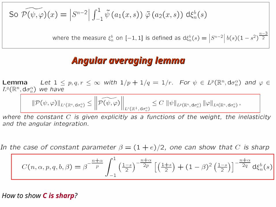
Angular averaging lemmaAngular averaging lemma

How to show C is sharp?

so and

Then , define the following bilinear operator for any two bounded and continuous functions f, g :+ ,

The radial symmetrization method generated the “extremal” operator for x ϵ +

Following Beckner’s approach ’75 Brascamp Lieb 76, one can find show C if the “best” constant by finding a pair sequence of functions such the operator acting on them achieves it.

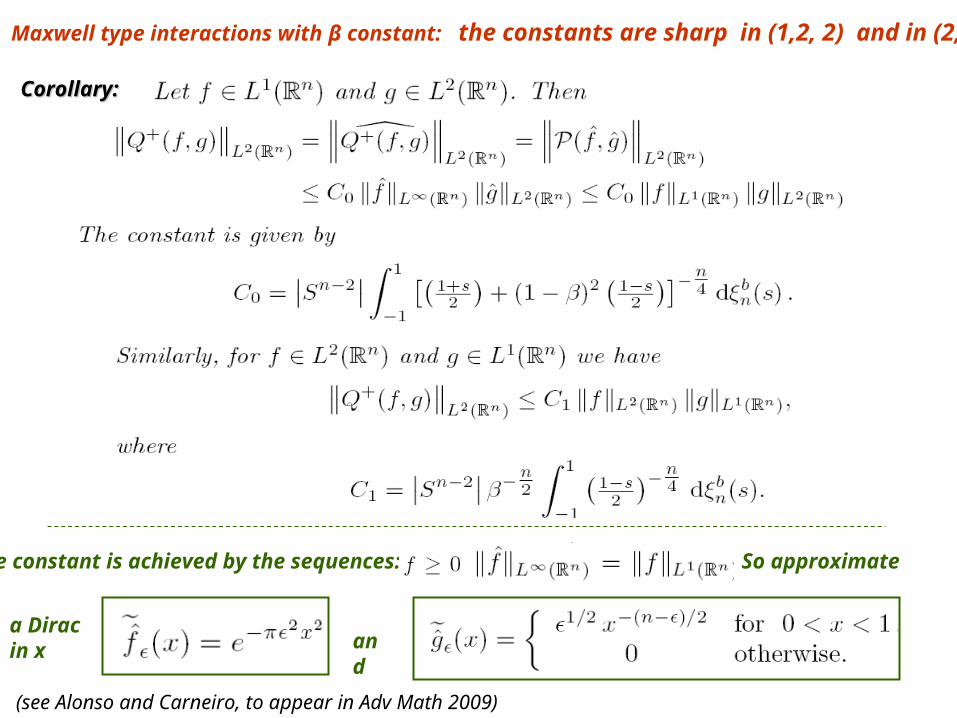
Maxwell type interactions with β constant: the constants are sharp in (1,2, 2) and in (2,1,2)

Corollary:Corollary:

The constant is achieved by the sequences:

and

So approximate

a Dirac in x

(see Alonso and Carneiro, to appear in Adv Math 2009)

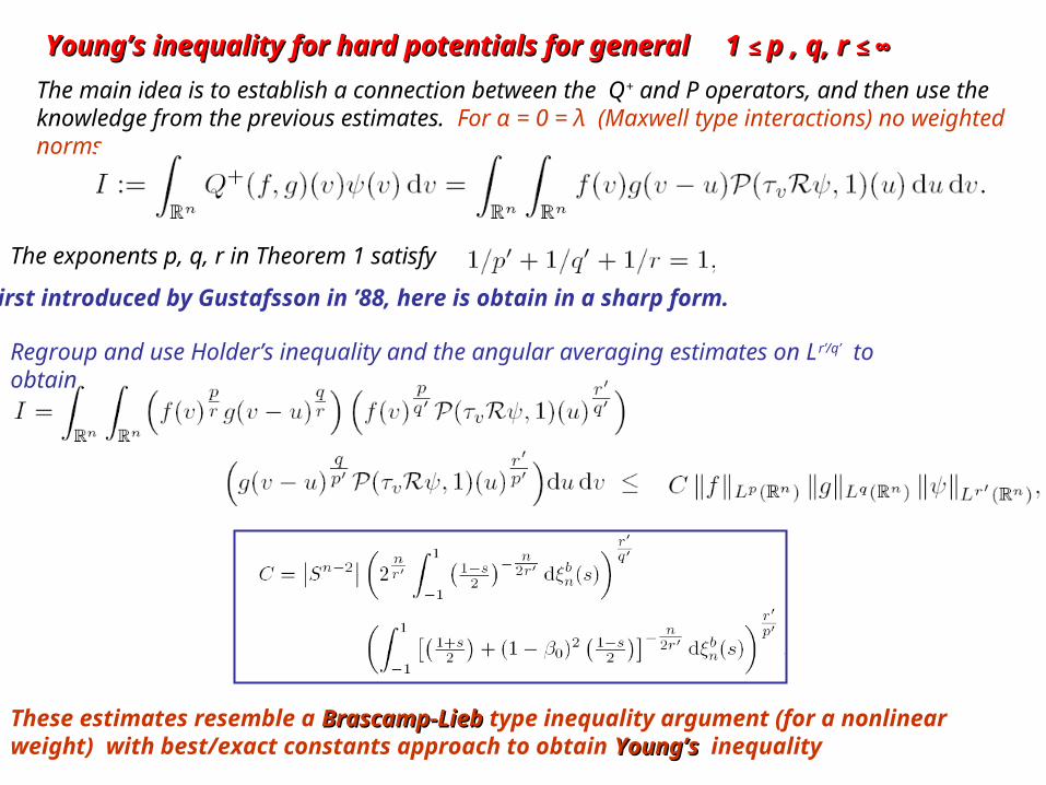
Young’s inequality for hard potentials for general 1 Young’s inequality for hard potentials for general 1 ≤ ≤ p , q, r p , q, r ≤ ∞≤ ∞

The main idea is to establish a connection between the Q+ and P operators, and then use the knowledge from the previous estimates. For α = 0 = λ (Maxwell type interactions) no weighted norms

The exponents p, q, r in Theorem 1 satisfy

Regroup and use Holder’s inequality and the angular averaging estimates on L r’/q’ to obtain

These estimates resemble a Brascamp-LiebBrascamp-Lieb type inequality argument (for a nonlinear weight) with best/exact constants approach to obtain Young’sYoung’s inequality

First introduced by Gustafsson in ’88, here is obtain in a sharp form.

2- Young’s inequality for hard potentials with |v|α weights with α + λ >0: For

Then, one obtains

1-

2-

3-

As in the previous case, by Holder and the unitary transformations

all with the same

Remark: 1- Previous LP estimates by Gustafsson 88, Villani-Mouhot ‘04 for pointwise bounded b(u . σ),I.M.G-Panferov-Villani ’03 for (p,1,p) with σ -integrable b(u . σ) in Sn-1. 2-The dependence on the weight α may have room to improvement. One may expect estimates with polynomial (?) decay in α , like in L1

α as shown Bobylev,I.M.G, Panferov and recently with Villani (97, 04,08)(also previous work of Wennberg ’94, Desvilletes, 96, without decay rates.)

Hardy-Littlewood-Sobolev inequality for soft potentials -n < Hardy-Littlewood-Sobolev inequality for soft potentials -n < λλ < 0 : < 0 :

Applying Holder’s inequality and then the angular averaging lemma to the inner integral with (p, q, r) = (a,1, a), a to be determined, one obtains

The choice of integrability exponents allowed to get rid of the integrand singularity at s = −1, producing a uniform control with respect to the inelasticity β.

Indeed, combining with the complete integral above, using triple Holder’s inq. yields

Is it possible to make such choice of a ?

Also here estimates resemble a Brascamp-LiebBrascamp-Lieb type inequality argument (for a nonlinear weight)

Then: for

Using the classical Hardy-Littlewood-Sobolev inequality to obtain (Lieb ’83)

where the exponents satisfy

In fact, it is possible to find 1/a in the non-empty interval

such that

for

and

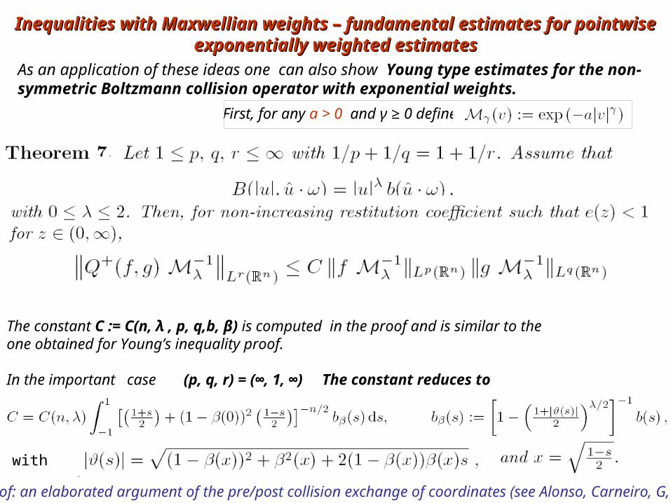
Inequalities with Maxwellian weights – fundamental estimates for pointwise exponentially Inequalities with Maxwellian weights – fundamental estimates for pointwise exponentially weighted estimatesweighted estimates

As an application of these ideas one can also show Young type estimates for the non-symmetric Boltzmann collision operator with exponential weights.

First, for any a > 0 and γ ≥ 0 define

The constant C := C(n, λ , p, q,b, β) is computed in the proof and is similar to the one obtained for Young’s inequality proof.

In the important case (p, q, r) = (∞, 1, ∞) The constant reduces to

with

Proof: an elaborated argument of the pre/post collision exchange of coordinates (see Alonso, Carneiro, G, 09)

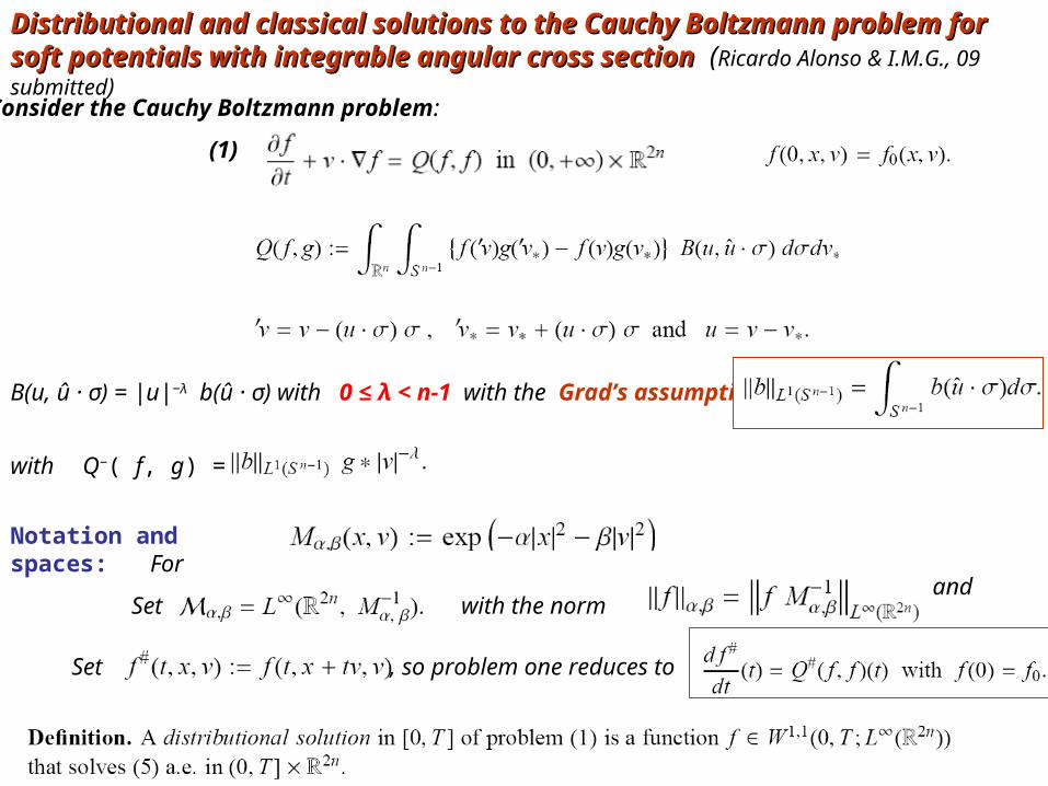
Consider the Cauchy Boltzmann problem:

B(u, û · σ) = |u|−λ b(û · σ) with 0 ≤ λ < n-1 with the Grad’s assumption:

Q−( f, g) = f

Distributional and classical solutions to the Cauchy Boltzmann problem for soft potentials Distributional and classical solutions to the Cauchy Boltzmann problem for soft potentials with integrable angular cross sectionwith integrable angular cross section (Ricardo Alonso & I.M.G., 09 submitted)

with

Notation and spaces: For

Set with the norm

(1)

and

Set , so problem one reduces to

Kaniel & Shinbrot iteration ’78: define the sequences {ln(t)} and {un(t)} as the mild solutions to (also Illner & Shinbrot ’83)

which relies in choosing a pair of functions (l0, u0) satisfying so called the beginning condition in [0, T]:

and

Theorem: Let {ln(t)} and {un(t)} the sequences defined by the mild solutions of the linear system above,such that the beginning condition is satisfied in [0, T], then

(i) The sequences {ln(t)} and {un(t)} are well defined for n ≥ 1. In addition, {ln(t)}, {un(t)} areincreasing and decreasing sequences respectively, and

l#n (t) ≤ u#

n (t) a.e. in 0 ≤ t ≤ T.

(ii) If 0 ≤ ln(0) = f0 = un(0) for n ≥ 1, then

The limit f (t) ∈ C(0, T; M#α,β) is the unique distributional solution of the Boltzmann equation in [0, T] and

fulfills 0 ≤ l#

0(t) ≤ f #(t) ≤ u#0(t) a.e. in [0, T].

Lemma : Assume −1 ≤ λ < n − 1. Then, for any 0 ≤ s ≤ t ≤ T and functions f #, g# that lie in L∞(0, T;M#

α,β), then the following inequality holds

with

So the following statement holds: Distributional solutions for small initial data: (near vacuum)

Theorem: Let B(u, û · σ) = |u|−λ b(û · σ) with -1 ≤ λ < n-1 with the Grad’s assumption Then, the Boltzmann equation has a unique global distributional solution if

. Moreover for any T ≥ 0 ,

As a consequence, one concludes that the distributional solution f is controlled by a traveling Maxwellian, and that

Hard and soft potentials case for small initial data

It behaves like the heat equation, asmass spreads as t grows

## ##

##

Theorem: Let B(u, û · σ) = |u|−λ b(û · σ) with -n < λ ≤ 0 with the Grad’s assumption In addition, assume that f0 is ε–close to the local Maxwellian distribution M(x, v) = C Mα,β(x − v, v) (0 < α, 0 < β). Then, for sufficiently small ε the Boltzmann equation has a unique solution satisfying

C1(t) Mα1,β1 (x − (t + 1)v, v ) ≤ f ( t, x-vt , v) ≤ C2(t) Mα2,β2

(x − (t + 1)v, v)

for some positive functions 0 < C1(t) ≤ C ≤ C2(t) < ∞, and parameters 0 < α2 ≤ α ≤ α1 and0 < β2 ≤ β ≤ β1.

Moreover, the case β = 0 (infinite mass) is permitted as long as β1 = β2 = 0.(this last part extends the result of Mishler & Perthame ’97 to soft potentials)

Distributional solutions near local Maxwellians :Distributional solutions near local Maxwellians : Ricardo Ricardo Alonso, IMG’08Alonso, IMG’08 Previous work by Toscani ’88, Goudon’97, Mischler –Perthame ‘97

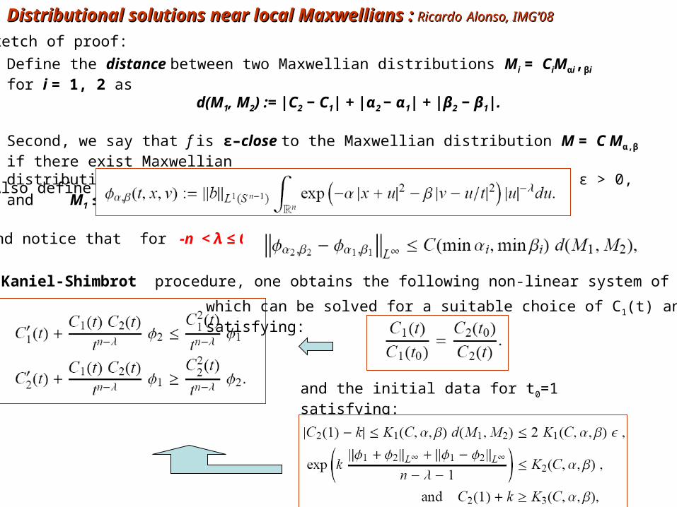
Distributional solutions near local Maxwellians :Distributional solutions near local Maxwellians : Ricardo Ricardo Alonso, IMG’08Alonso, IMG’08

Define the distance between two Maxwellian distributions Mi = CiMαi,βi

for i = 1, 2 as d(M1, M2) := |C2 − C1| + |α2 − α1| + |β2 − β1|.

Second, we say that f is ε–close to the Maxwellian distribution M = C Mα,β if there exist Maxwelliandistributions Mi (i = 1, 2) such that d(Mi, M) <ε for some small ε > 0, and M1 ≤ f ≤ M2.

Also define

and notice that for -n < λ ≤ 0

Following the Kaniel-Shimbrot procedure, one obtains the following non-linear system of inequations

which can be solved for a suitable choice of C1(t) and C2(t)satisfying:

and the initial data for t0=1 satisfying:

Sketch of proof:

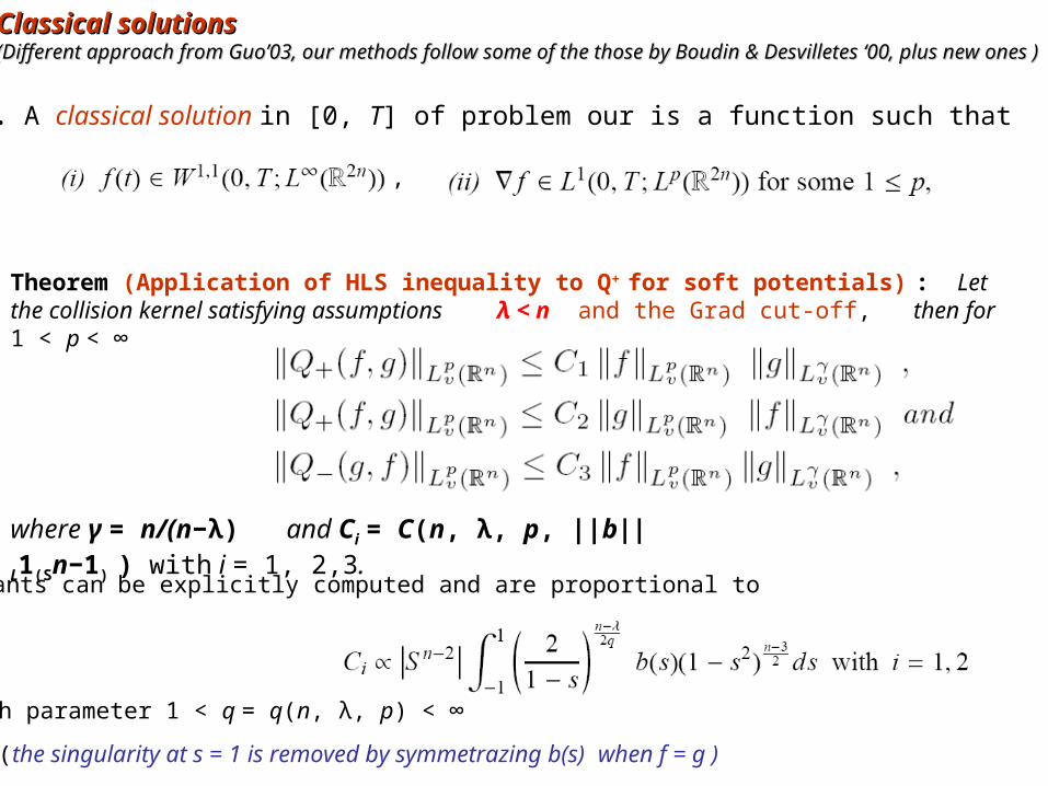
Classical solutions Classical solutions (Different approach from Guo’03, our methods follow some of the those by Boudin & Desvilletes ‘00, plus new ones ) (Different approach from Guo’03, our methods follow some of the those by Boudin & Desvilletes ‘00, plus new ones )

Definition. A classical solution in [0, T] of problem our is a function such that

,

Theorem (Application of HLS inequality to Q+ for soft potentials) : Let the collision kernel satisfying assumptions λ < n and the Grad cut-off, then for 1 < p < ∞

where γ = n/(n−λ) and Ci = C(n, λ, p, ||b||L1(Sn−1) ) with i = 1, 2,3.

The constants can be explicitly computed and are proportional to

with parameter 1 < q = q(n, λ, p) < ∞

(the singularity at s = 1 is removed by symmetrazing b(s) when f = g )

Theorem (global regularity near Maxwellian data) Fix 0 ≤ T ≤ ∞ and assume the collision kernel satisfies B(u, û · σ) = |u|−λ b(û · σ) with -1 ≤ λ < n-1 with the Grad’s assumption.

Also, assume that f0 satisfies the smallness assumption or is near to a local Maxwellian. In addition, assume that ∇f0 ∈ Lp(R2n) for some 1 < p < ∞. Then, there is a unique classical solution f to problem (1) in the interval [0, T] satisfying the estimates of these theorems, and for all t [0, ∈ T],

with constant

Proof: set

: ∫

with

By Gronwall inequality

with a = n/(n−λ)

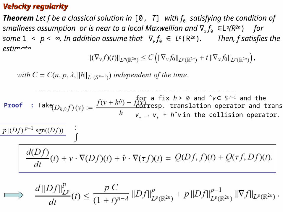
Velocity regularityVelocity regularity

Proof : Take for a fix h > 0 and ˆv ∈ S n−1 and the corresp. translation operator and transforming

v∗ → v∗ + hˆv in the collision operator.

: ∫

Theorem Let f be a classical solution in [0, T] with f0 satisfying the condition of smallness assumption or is near to a local Maxwellian and ∇x f0 L∈ p(R2n) for some 1 < p < ∞. In addition assume that ∇v f0 ∈ Lp(R2n). Then, f satisfies the estimate

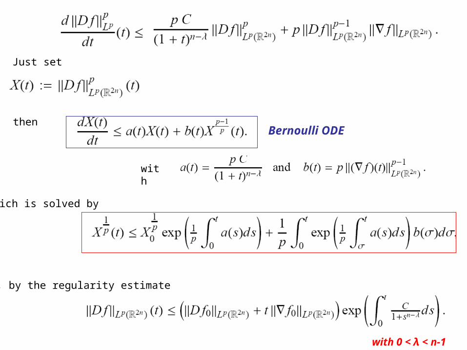
with

then

Which is solved by

Just set

Then, by the regularity estimate

with 0 < λ < n-1

Bernoulli ODE

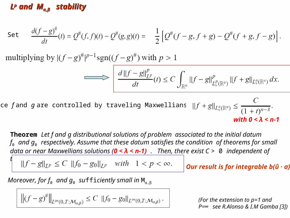
LLpp and M and Mα,βα,β stability stability

Set

Now, since f and g are controlled by traveling Maxwellians one has

Theorem Let f and g distributional solutions of problem associated to the initial datumf0 and g0 respectively. Assume that these datum satisfies the condition of theorems for small data or near Maxwellians solutions (0 < λ < n-1) . Then, there exist C > 0 independent of time such that

Moreover, for f0 and g0 sufficiently small in Mα,β

Our result is for integrable b(û · σ)

with 0 < λ < n-1

(For the extension to p=1 and P=∞ see R.Alonso & I.M Gamba [3])

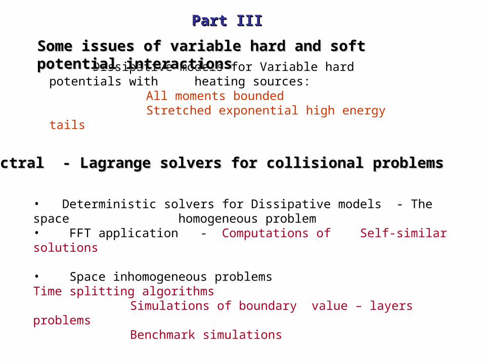
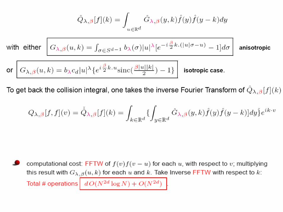
• Dissipative models for Variable hard potentials with heating sources:

All moments bounded Stretched exponential high energy tails

Some issues of variable hard and soft potential interactionsSome issues of variable hard and soft potential interactions

Spectral - Lagrange solvers for collisional problemsSpectral - Lagrange solvers for collisional problems

• Deterministic solvers for Dissipative models - The space homogeneous problem

• FFT application - Computations of Self-similar solutions

• Space inhomogeneous problems Time splitting algorithms

Simulations of boundary value – layers problemsBenchmark simulations

Part IIIPart III

A general form statistical transport : The space-homogenous BTE with external heating sources Important examples from mathematical physics and social sciences:

The termmodels external heating sources:

•background thermostat (linear collisions), •thermal bath (diffusion)•shear flow (friction), •dynamically scaled long time limits (self-similar solutions).

Inelastic Collision u’= (1-β) u + β |u| σ , with σ the direction of elastic post-collisional relative velocity

‘v

‘v*

v

v*

η inelastic collision

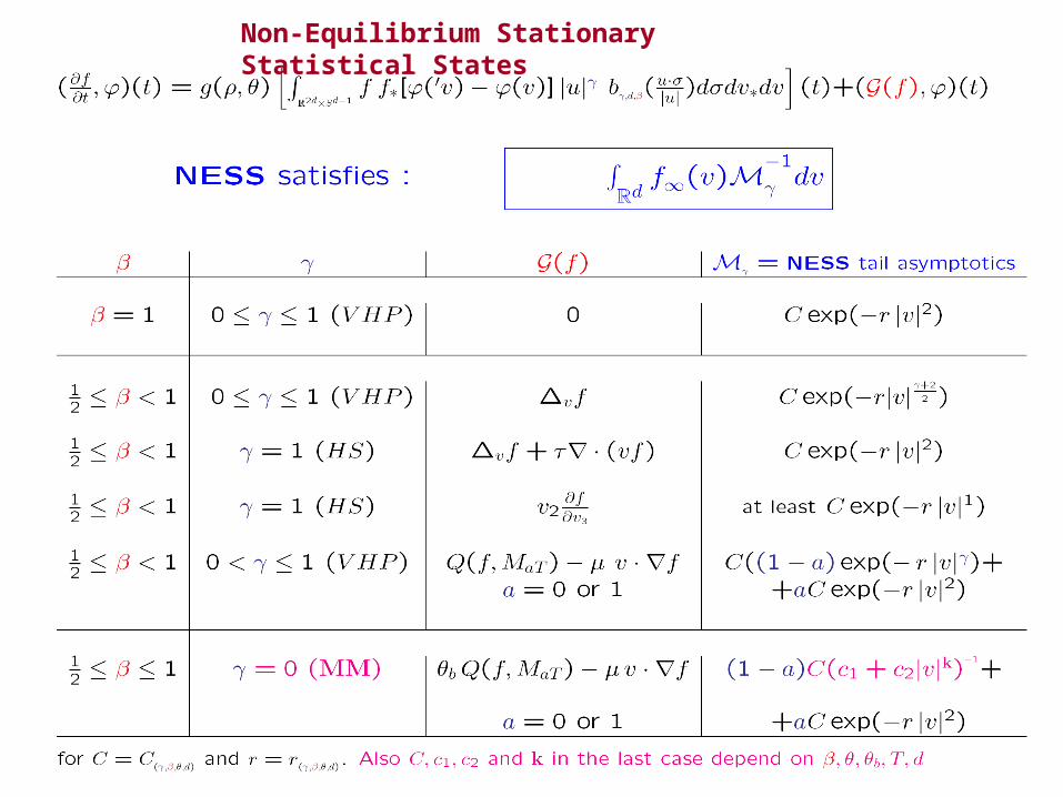
Non-Equilibrium Stationary Statistical States

Spectral - Lagrange solvers for collisional problemsSpectral - Lagrange solvers for collisional problems

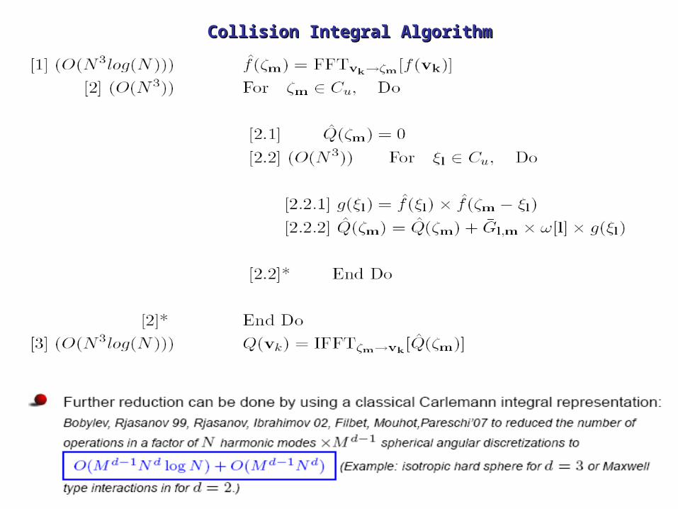
Collision Integral AlgorithmCollision Integral Algorithm

~

~

~

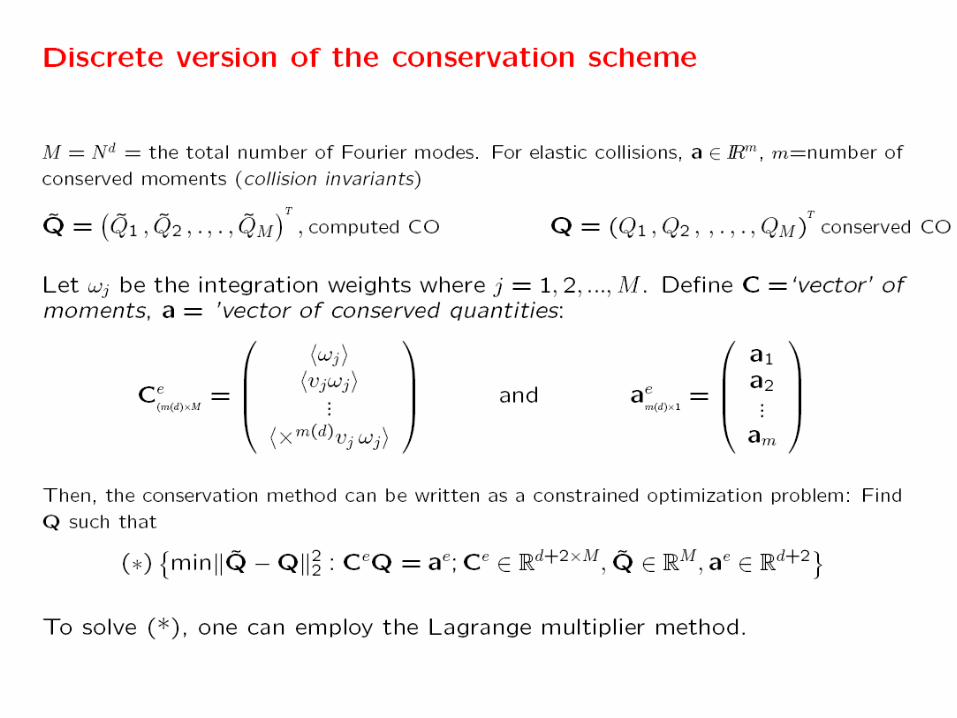
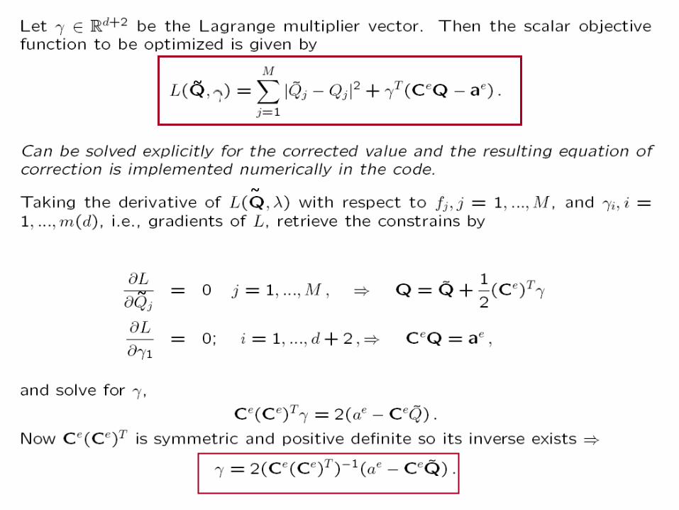
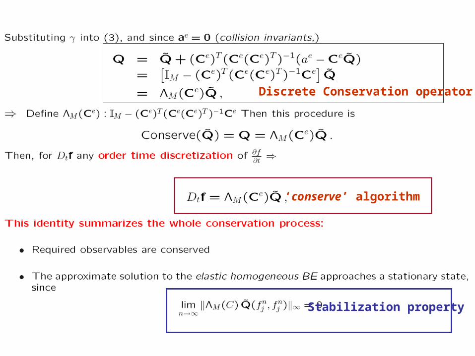
‘conserve’ algorithm

Stabilization property

Discrete Conservation operator

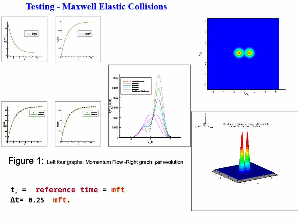
tr = reference time = mft Δt= 0.25 mft.

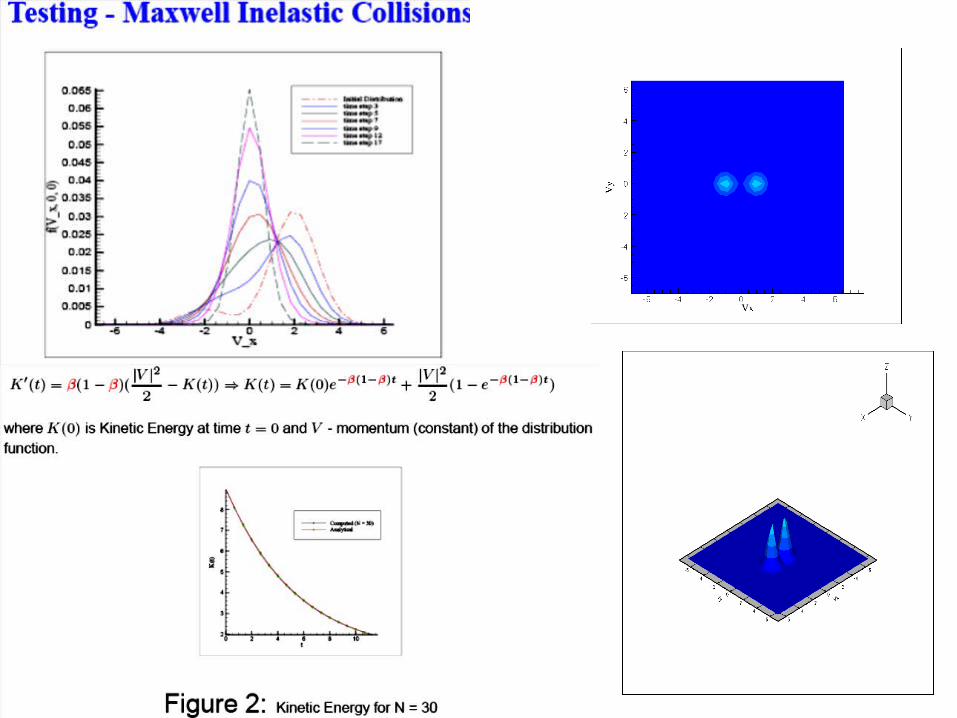
Soft condensed matter Soft condensed matter phenomenaphenomena

Remark: The numerical algorithm is based on the evolution of the continuous spectrum of the solution as in Greengard-Lin’00 spectral calculation of the free space heat kernel, i.e. self-similar of the heat equation in all space.

Isomoment estimatesIsomoment estimates

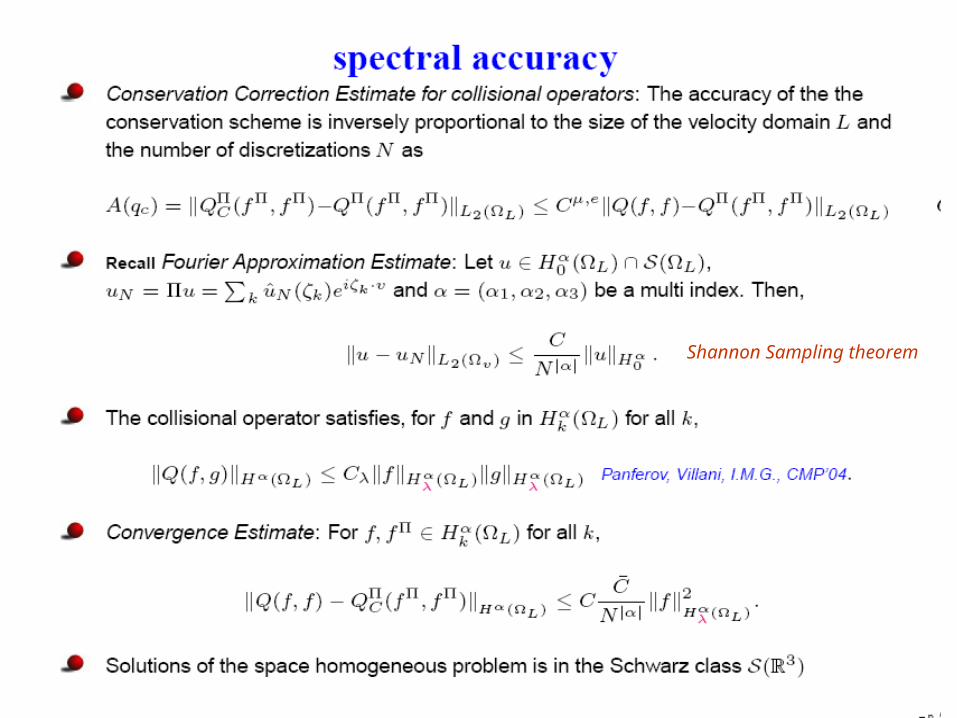
Shannon Sampling theorem

Space inhomogeneous simulationsSpace inhomogeneous simulationsmean free time := the average time between collisionsmean free path := average speed x mft (average distance traveled between collisions) Set the scaled equation for 1= Kn := mfp/geometry of length scale

Spectral-Lagrangian methods in 3D-velocity space and 1D physical space discretization in the simplest setting:

N= Number of Fourier modes in each j-direction in 3D

Spatial mesh size Δx = O.O1 mfp Time step Δt = r mft , mft= reference time

Resolution of discontinuity ’near the wall’ for diffusive boundary conditions:Resolution of discontinuity ’near the wall’ for diffusive boundary conditions: (K.Aoki, Y. Sone, K. Nijino, H. Sugimoto, 1991)

Sudden heatingSudden heating:: Constant moments initial state with a discontinuous pdf at the boundary wall, with wall kinetic temperature increased by twice its magnitude:

Calculations in the next two pages: Mean free path l0 = 1. Number of Fourier modes N = 243, Spatial mesh size Δx = 0.01 l0 . Time step Δt = r mft

Boundary Conditions for sudden heating:

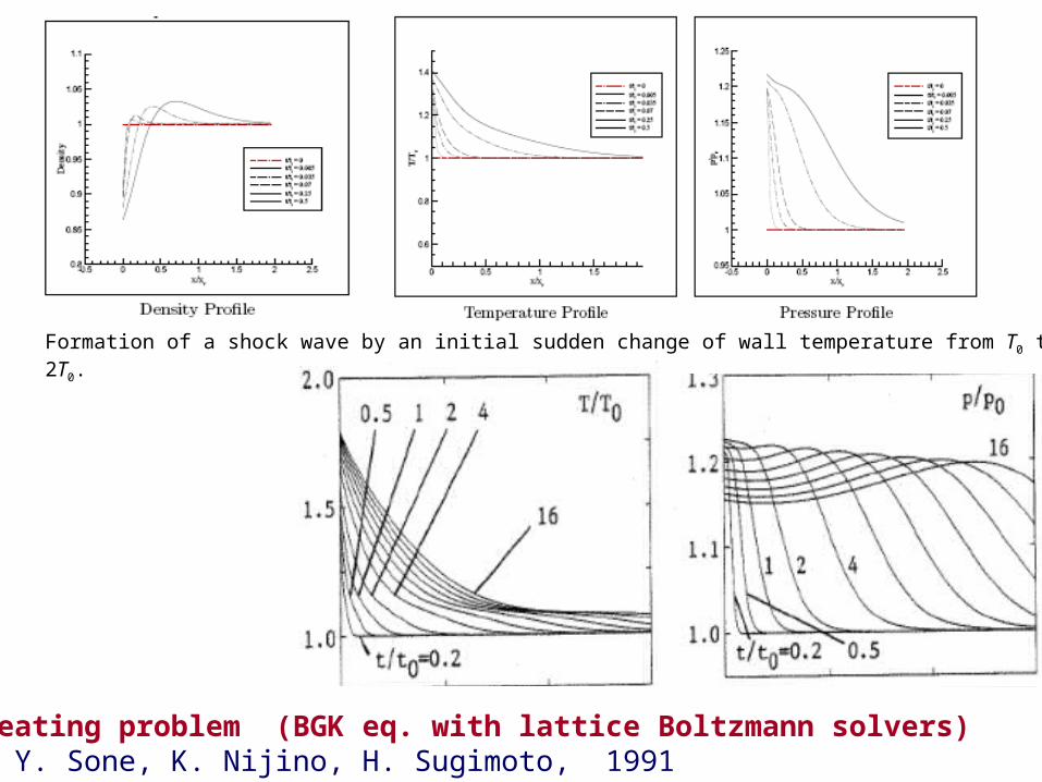
Formation of a shock wave by an initial sudden change of wall temperature from T0 to 2T0.

Sudden heating problem (BGK eq. with lattice Boltzmann solvers) K.Aoki, Y. Sone, K. Nijino, H. Sugimoto, 1991

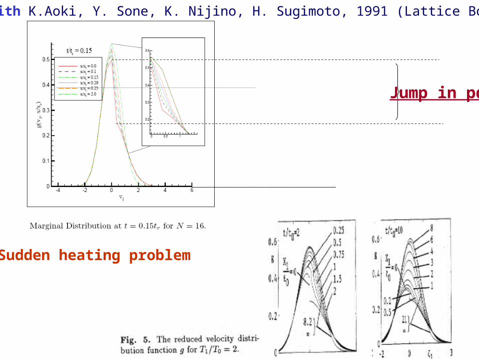
Jump in pdf

Comparisons with K.Aoki, Y. Sone, K. Nijino, H. Sugimoto, 1991 (Lattice Boltzmann on BGK)

Sudden heating problem

Temperature: T0 given at xo=0 and T1 = 2T0 at x1 = 1.

Knudsen Kn = 0.1, 0.5, 1, 2, 4

Heat transfer problem:

Diffusive boundary conditions

References1. R.J. Alonso and E. Carneiro, Estimates for the Boltzmann collision operator via radial symmetry and

Fourier transform, Adv. Math., to appear.2. *R.J. Alonso, E. Carneiro and I.M. Gamba, Convolution inequalities for the Boltzmann collision

operator, arXiv:0902.0507v2, submitted. (2009)3. R.J. Alonso and I.M. Gamba, L1 −L1-Maxwellian bounds for the derivatives of the solution of the

homogeneous Boltzmann equation. Journal de Math.Pures et Appl.,(9) 89 (2008), no. 6, 575–595.4. *R.J. Alonso and I.M. Gamba, Distributional and classical solutions to the Cauchy-Boltzmann5. problem for soft potentials with integrable angular cross section arXiv:0902.3106v2, submitted. (2009)6. W. Beckner, Inequalities in Fourier analysis, Ann. of Math. (2) 102 (1975), no. 1, 159–182.7. Bellomo, N. and Toscani, G.: On the Cauchy problem for the nonlinear Boltzmann equation: global

existence, uniqueness and asymptotic behavior. J. Math. Phys. 26, 334-338 (1985). 8. A. Bobylev, The method of the Fourier transform in the theory of the Boltzmann equation for Maxwell

molecules, Dokl. Akad. Nauk SSSR 225 (1975), no. 6, 1041–1044.9. A. Bobylev, J.A.Carrillo and I. M. Gamba, On some properties of kinetic and hydrodynamic equations

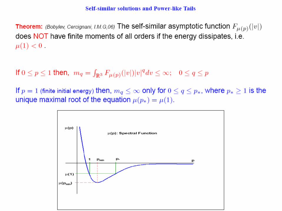
for inelastic interactions. J. Statist. Phys. 98 (2000), no. 3-4, 743-773.10. A. Bobylev, C. Cercignani and I. M. Gamba, On the self-similar asymptotics for generalized non-linear

kinetic Maxwell models, to appear in Comm. Math.Phys. (2009).11. A. Bobylev and I.M.Gamba, Boltzmann equations for mixtures of Maxwell gases: exact solutions and

power like tails. J. Stat. Phys. 124, no. 2-4, 497--516. (2006).12. A. Bobylev, I. M. Gamba and V. Panferov, Moment inequalities and high-energy tails for Boltzmann

equations with inelastic interactions, J. Statist. Phys. 116 (2004), 1651–1682.13. Boudin, L. and Desvillettes, L.: On the singularities of the global small solutions of the full Boltzmann

equation. Monatsh. Math. 131, 91-108 (2000).14. H. J. Brascamp, E. Lieb and J. M. Luttinger, A general rearrangement inequality for multiple integrals,

J. Functional Analysis 17 (1974), 227–237. 15. H. J. Brascamp, E. Lieb Best constants in Young’s inequality, its converse, and its generalization to

more than three functions, Adv. Math. 20 (1976),16. N. Brilliantov and T. Pöschel, Kinetic theory of granular gases, Oxford Univ. Press, (2004).17. Burchard, A. A Short Course on Rearrangement Inequalities, http://www.math.toronto.edu/almut/rearrange.pdf

18. Caflisch, R.: The Boltzmann equation with a soft potential (II). Comm. Math. Phys. 74, 97-109 (1980).19. C. Cercignani, R. Illner and M. Pulvirenti, The mathematical theory of dilute gases, Applied

Mathematical Sciences, vol. 106, Springer-Verlag, New York, 1994.20. L. Desvillettes, About the use of the Fourier transform for the Boltzmann equation, Riv. Mat. Univ.

Parma. 7 (2003), 1–99.

21. R. Duduchava, R. Kirsch and S. Rjasanow, On estimates of the Boltzmann collision operator with cutoff, J. Math. Fluid Mech. 8 (2006), no. 2, 242–266

22. I. M. Gamba, V. Panferov and C. Villani, Upper Maxwellian bounds for the spatially homogeneous Boltzmann equation, Arch. Rational Mech. Anal. (2009).

23. I. M. Gamba, V. Panferov and C. Villani, On the Boltzmann equation for diffusively excited granular media, Comm. Math. Phys. 246 (2004), no. 3, 503–541.

24. *I. M. Gamba and Sri Harsha Tharkabhushaman, Spectral - Lagrangian based methods applied to computation of Non - Equilibrium Statistical States. Jour. Computational Physics, (2009)

25. *I.M.Gamba and Harsha Tarskabhushanam Shock and Boundary Structure formation by Spectral Lagrangian methods for the Inhomogeneous Boltzmann Transport Equation, to appear in JCM’09

26. Gardner, Richard J. (2002). "The Brunn–Minkowski inequality". Bull. Amer. Math. Soc. (N.S.) 39 (3): pp. 355–405

27. Glassey, R.:Global solutions to the Cauchy problem for the relativistic Boltzmann equation with near-vacuum data. Comm. Math. Phys. 264, 705-724 (2006).

28. Goudon, T.: Generalized invariant sets for the Boltzmann equation. Math. Models Methods Appl. Sci. 7, 457-476 (1997)

29. T. Gustafsson, Global Lp properties for the spatially homogeneous Boltzmann equation, Arch. Rational Mech. Anal. 103 (1988), 1–38

30. Ha, S.-Y.: Nonlinear functionals of the Boltzmann equation and uniform stability estimates. J. Di. Equat. 215, 178- 05 (2005)

31. Ha, S.-Y. and Yun S.-B.: Uniform L1-stability estimate of the Boltzmann equation near a local Maxwellian. Phys.Nonlinear Phenom. 220, 79{97 (2006)

32. Hamdache, K.: Existence in the large and asymptotic behavior for the Boltzmann equation. Japan. J. Appl. Math. 2, 1-15 (1985)

33. Illner, R. and Shinbrot, M.: The Boltzmann equation, global existence for a rare gas in an innite vacuum. Commun. Math. Phys. 95, 217-226 (1984).

34. Kaniel, S. and Shinbrot, M.: The Boltzmann equation I. Uniqueness and local existence. Commun. Math. Phys. 58, 65-84 (1978).

35. E. H. Lieb, Sharp constants in the Hardy-Littlewood-Sobolev and related inequalities, Ann. of Math. (2) 118 (1983), no. 2, 349–374.

36. E. H. Lieb and M. Loss, Analysis, Graduate Studies in Mathematics, v. 14 (2001), American Mathematical Society, Providence, RI.

37. S. Mischler, C. Mouhot and M. R. Ricard, Cooling process for inelastic Boltzmann equations for hard spheres. Part I: The Cauchy problem, J. Statist. Phys. 124 (2006), 655-702.

38. C. Mouhot and C. Villani, Regularity theory for the spatially homogeneous Boltzmann equation with cut-off, Arch. Rational Mech. Anal. 173 (2004), 169–212.

39. Mischler, S. and Perthame, B.: Boltzmann equation with innite energy: renormalized solutions and distributional solutions for small initial data and initial data close to Maxwellian. SIAM J. Math. Anal. 28, 1015-1027 (1997).

40. Palczewski, A. and Toscani, G.: Global solution of the Boltzmann equation for rigid spheres and initial data close to a local Maxwellian. J. Math. Phys. 30, 2445-2450 (1989)

41. Toscani, G.: Global solution of the initial value problem for the Boltzmann equation near a local Maxwellian . Arch. Rational Mech. Anal. 102, 231-241 (1988).

42. Ukai, S. and Asano, K.: On the Cauchy problem of the Boltzmann equation with a soft potential. Publ. Res. Inst. Math. Sci. 18, 477-519(57-99) (1982).

43. Villani, C.: On a new class of weak solutions to the spatially homogeneous Boltzmann and Landau equations. Arch. Rational. Mech. Anal. 143, 273-307 (1998).

44. C. Villani, A review of mathematical topics in collisional kinetic theory, Handbook of mathematical fluid dynamics, Vol. I, 71–305, North-Holland, Amsterdam, 2002.

References and preprints http://rene.ma.utexas.edu/users/gamba/publications-web.htm

Muchas gracias por su atención