Probing Bloch band geometry with ultracold atoms in...
149
Probing Bloch band geometry with ultracold atoms in optical lattices Tracy Li München 2016
Transcript of Probing Bloch band geometry with ultracold atoms in...

Probing Bloch band geometry withultracold atoms in optical lattices
Tracy Li
München 2016

Probing Bloch band geometry withultracold atoms in optical lattices
Tracy Li
Dissertationan der Fakultät für Physik
der Ludwig–Maximilians–UniversitätMünchen
vorgelegt vonTracy Li
aus Nanjing, China
München, Mai 2016

Erstgutachter: Prof. I. Bloch
Zweitgutachter: Prof. E. Demler
Weitere Prüfungskommissionsmitglieder: Prof. A. Högele, Prof. U. Schollwöck
Tag der mündlichen Prüfung: 13. Juli 2016
Zusammenfassung
Zusammenfassung
Ultrakalte Atome in optischen Gittern haben sich unlängst als vielversprechendes Mit-tel zur Untersuchung geometrischer und topologischer Aspekte von Bandstrukturenerwiesen. In dieser Arbeit werden wir das hohe Maß an Kontrolle, das diese Systeme er-möglichen, ausnutzen, um die Bandgeometrie eines hexagonalen optischen Gitters zuuntersuchen. In der ersten Reihe von Experimenten realisieren wir ein Atominterfer-ometer im Quasiimpulsraum, um den singulären Berryfluss zu messen, der mit einemDirakpunkt assoziiert ist. Diese Technik erlaubt es uns, die Verteilung der Berrykrüm-mung in der Brillouinzone mit sehr hoher Quasiimpulsauflösung zu bestimmen. AlsNächstes realisieren wir Dynamiken, die durch sehr starke Kräfte erzeugt werden unddie mithilfe von Wilsonlinien beschrieben werden können. Diese Wilsonlinien wer-den durch Matrizen dargestellt und sind eine Verallgemeinerung der Berryphase fürentartete Systeme. Wir zeigen, dass aus der Entwicklung der Bandpopulationen indiesem Regime direkt die Bandgeometrie abgeleitet werden kann. Diese Methodeermöglicht die Rekonstruktion der zellenperiodischen Blochzustände für alle Quasi-impulse sowie der Eigenwerte der Wilson-Zak-Schleifen. Unsere Techniken könnengenutzt werden, um topologische Invarianten zu bestimmen, die die Bandstrukturcharakterisieren, wie zum Beispiel die Chernnummer und dieZ2 Nummer. Aufbauendauf diesen Ergebnissen präsentieren wir abschließend vorläufige Experimente zur Ma-nipulation von Bandstrukturen.
Abstract
Ultracold atoms in optical lattices have recently emerged as promising candidates forinvestigating the geometric and topological aspects of band structures. In this thesis,we exploit the high degree of control available in these systems to directly probe theband geometry of an optical honeycomb lattice. In the first series of experiments, werealize an atomic interferometer in quasimomentum space to measure the singularBerry flux associated with a Dirac point. This technique enables us to determine thedistribution of Berry curvature in the Brillouin zone with high quasimomentum res-olution. Next, we realize strong-force dynamics that are described by matrix-valuedWilson lines, which are generalizations of the Berry phase to degenerate systems. Inthis strong-force regime, we show that the evolution in the band populations directlyreveals the band geometry. This method enables the reconstruction of both the cell-periodic Bloch states at every quasimomentum and the eigenvalues of Wilson-Zakloops. Our techniques can be used to determine the topological invariants, such asthe Chern andZ2 numbers, that characterize the band structure. Lastly, having estab-lished our ability to detect the band geometry, we present preliminary experiments onengineering band structures.
v

Contents
1. Introduction 1
2. Geometric quantities in Bloch bands 72.1. Geometric phases in brief . . . . . . . . . . . . . . . . . . . . . . . . . . . . . 72.2. Accessing geometric properties in Bloch bands . . . . . . . . . . . . . . . . 10
2.2.1. Preliminaries . . . . . . . . . . . . . . . . . . . . . . . . . . . . . . . . 102.2.2. Derivation of the equations of motion . . . . . . . . . . . . . . . . . . 122.2.3. Adiabatic motion: the Berry phase . . . . . . . . . . . . . . . . . . . . 132.2.4. Diabatic motion: the Wilson line . . . . . . . . . . . . . . . . . . . . . 15
2.3. Gauge invariance: which quantities are measurable? . . . . . . . . . . . . . 162.3.1. Single-band geometric quantities . . . . . . . . . . . . . . . . . . . . 162.3.2. Multi-band geometric quantities . . . . . . . . . . . . . . . . . . . . . 172.3.3. A summary . . . . . . . . . . . . . . . . . . . . . . . . . . . . . . . . . . 18
2.4. A blueprint for the experiments . . . . . . . . . . . . . . . . . . . . . . . . . . 19
3. The optical honeycomb lattice 213.1. The tight-binding model . . . . . . . . . . . . . . . . . . . . . . . . . . . . . . 21
3.1.1. ∆= 0: Dirac points and Berry phases . . . . . . . . . . . . . . . . . . 243.1.2. ∆ 6= 0: Effect of the Semenoff mass and the Bloch sphere picture . . 26
3.2. The ab-initio calculation . . . . . . . . . . . . . . . . . . . . . . . . . . . . . . 303.2.1. Setting up the problem . . . . . . . . . . . . . . . . . . . . . . . . . . . 303.2.2. Application to the optical honeycomb potential . . . . . . . . . . . . 313.2.3. Energy bands from the ab-initio calculation . . . . . . . . . . . . . . 33
4. An overview of the experimental setup 374.1. Creation of the optical honeycomb lattice . . . . . . . . . . . . . . . . . . . 38
4.1.1. The optical dipole potential . . . . . . . . . . . . . . . . . . . . . . . . 384.1.2. The ideal optical honeycomb lattice . . . . . . . . . . . . . . . . . . . 394.1.3. Modifications on the ideal: non-isotropic tunneling and adding a
Semenoff mass . . . . . . . . . . . . . . . . . . . . . . . . . . . . . . . 414.2. State preparation: creating a BEC . . . . . . . . . . . . . . . . . . . . . . . . . 444.3. State evolution: creating a gradient . . . . . . . . . . . . . . . . . . . . . . . 45
4.3.1. Magnetic field . . . . . . . . . . . . . . . . . . . . . . . . . . . . . . . . 464.3.2. Lattice acceleration . . . . . . . . . . . . . . . . . . . . . . . . . . . . . 46
vii
Contents
4.4. State detection: absorption imaging . . . . . . . . . . . . . . . . . . . . . . . 484.4.1. Sudden shut-off of the lattice: plane-wave decomposition . . . . . . 494.4.2. Ramp-down of the lattice: band mapping . . . . . . . . . . . . . . . 51
4.5. Applications: Bloch oscillations and lattice depth calibration . . . . . . . . 544.5.1. Bloch oscillations . . . . . . . . . . . . . . . . . . . . . . . . . . . . . . 544.5.2. Lattice calibration . . . . . . . . . . . . . . . . . . . . . . . . . . . . . 56
5. Measuring the Berry phase 595.1. An analogy with the Aharonov-Bohm effect . . . . . . . . . . . . . . . . . . 595.2. The experimental procedure . . . . . . . . . . . . . . . . . . . . . . . . . . . 60
5.2.1. The sequence . . . . . . . . . . . . . . . . . . . . . . . . . . . . . . . . 615.2.2. Experimental parameters . . . . . . . . . . . . . . . . . . . . . . . . . 635.2.3. Experimental caveats . . . . . . . . . . . . . . . . . . . . . . . . . . . . 64
5.3. Experimental results . . . . . . . . . . . . . . . . . . . . . . . . . . . . . . . . 665.3.1. Detecting the Berry flux . . . . . . . . . . . . . . . . . . . . . . . . . . 675.3.2. Self-referenced interferometry near the Dirac point . . . . . . . . . 685.3.3. Moving and annihilating Dirac cones . . . . . . . . . . . . . . . . . . 69
6. Bloch state tomography with Wilson lines 736.1. Wilson lines in the s-bands of the honeycomb lattice . . . . . . . . . . . . . 74
6.1.1. Wilson-Zak loop eigenvalues . . . . . . . . . . . . . . . . . . . . . . . 746.1.2. Bloch state tomography . . . . . . . . . . . . . . . . . . . . . . . . . . 74
6.2. Reconstructing eigenstates: the Bloch sphere picture . . . . . . . . . . . . . 766.2.1. Extracting the polar angle θq . . . . . . . . . . . . . . . . . . . . . . . 776.2.2. Extracting the azimuthal angle φq . . . . . . . . . . . . . . . . . . . . 776.2.3. Gauge-invariance of φq and θq . . . . . . . . . . . . . . . . . . . . . . 79
6.3. Experimental details . . . . . . . . . . . . . . . . . . . . . . . . . . . . . . . . 806.3.1. Experimental parameters . . . . . . . . . . . . . . . . . . . . . . . . . 806.3.2. Reaching the strong gradient regime . . . . . . . . . . . . . . . . . . 816.3.3. The effect of higher bands . . . . . . . . . . . . . . . . . . . . . . . . . 836.3.4. Data analysis . . . . . . . . . . . . . . . . . . . . . . . . . . . . . . . . 83
6.4. Experimental results . . . . . . . . . . . . . . . . . . . . . . . . . . . . . . . . 856.4.1. Measuring θq . . . . . . . . . . . . . . . . . . . . . . . . . . . . . . . . 856.4.2. The real-space picture . . . . . . . . . . . . . . . . . . . . . . . . . . . 856.4.3. Measuring φq . . . . . . . . . . . . . . . . . . . . . . . . . . . . . . . . 88
6.5. Determining the Wilson-Zak loop eigenvalues . . . . . . . . . . . . . . . . . 896.5.1. Decomposition of the Wilson line into U (1) and SU (2). . . . . . . . 896.5.2. The back-tracking condition . . . . . . . . . . . . . . . . . . . . . . . 916.5.3. Wilson-Zak loop eigenvalues with and without inversion symmetry 926.5.4. Wilson-Zak loop eigenvalues and the real-space embedding . . . . 93
viii
Contents
7. Conclusion and Outlook 957.1. Outlook . . . . . . . . . . . . . . . . . . . . . . . . . . . . . . . . . . . . . . . . 96
7.1.1. Preliminary experiments . . . . . . . . . . . . . . . . . . . . . . . . . 987.1.2. Next steps . . . . . . . . . . . . . . . . . . . . . . . . . . . . . . . . . . 1017.1.3. Future endeavors . . . . . . . . . . . . . . . . . . . . . . . . . . . . . . 102
A. Experimental details 105A.1. The vacuum setup . . . . . . . . . . . . . . . . . . . . . . . . . . . . . . . . . 105
A.1.1. The magnetic transport coils and the experiment cell . . . . . . . . 107A.2. The laser setup . . . . . . . . . . . . . . . . . . . . . . . . . . . . . . . . . . . 110
A.2.1. Cooling in the 2D+-MOT and 3D-MOT . . . . . . . . . . . . . . . . . 110A.2.2. Optical dipole trap and lattice lasers . . . . . . . . . . . . . . . . . . . 111
A.3. The experimental sequence . . . . . . . . . . . . . . . . . . . . . . . . . . . . 112
B. Numerical calculation of the Wilson line 119
Bibliography 121
Acknowledgements 137
ix


Chapter 1.
Introduction
In condensed matter physics, band theory describes the approximation of the com-plex many-body problem of electrons in a solid by that of a single-particle in a pe-riodic potential [1]. At first glance, this approximation may seem unreasonably ex-treme, as it neglects all interaction effects and the inevitable impurities and deforma-tions present in any real solid. However, band theory has been remarkably successfulin describing a wide range of condensed matter phenomena and forms the founda-tion for our understanding of material properties. For example, the eigenvalues of thesingle-particle Schroedinger equation are discretely spaced for a given quasimomen-tum, forming bands of allowed energies. The collection of these bands forms a bandstructure and explains the difference between metals, insulators, and semiconductors.Although many insights can be derived from the energy bands alone, they are, how-ever, not the complete story. In 1980, the experimental discovery of the integer quan-tum Hall effect [2] propelled band theory in a new direction where the band eigenstatesand their geometric structure take center stage.
In the integer quantum Hall effect, the Hall conductivity of a 2D semiconductorat low temperatures and high magnetic fields is quantized in integer units of e2/h.Moreover, this quantization is remarkably robust to variations in the details of thedevice, such as its precise shape, material, or fabrication process [3]. In fact, al-ready in 1987, measurements in four different samples yielded the same results within5× 10−9 [4]. Presently, the Hall conductivity is particularly relevant for metrologicalapplications [3]: it has been measured to better than one part in a billion and is usedto define the standard of resistance [5].
The robust quantization in the integer quantum Hall effect is a hallmark of phenom-ena with topological underpinnings. In mathematics, the branch of topology aims togroup geometric objects into broad classes based on their global properties. For exam-ple, 2D surfaces are topologically classified by their genus, which counts the numberof holes. The genus can be expressed in terms of a topological invariant that is givenby the integral of the local curvature of the surface [6]. While the local curvature de-pends on the geometry, the total integral is independent of these details and reflectsthe topology of the object.
In condensed matter physics, there exist analogous topological invariants that de-
1
Chapter 1. Introduction
scribe the topology of the band eigenstates. For example, the integer quantum Halleffect is characterized by the TKNN invariant, which remarkably relates the Hall re-sponse to the topology of the band eigenstates [7]. Similar to the genus, the TKNNinvariant is obtained by integrating a local geometric quantity over the Brillouin zone;as before, while the integrand depends on details of the geometry, the final integraldoes not. The TKNN invariant, originally named after the authors Thouless, Kohmoto,Nightingale, and den Nijs who first formulated it, is also commonly called the Chernnumber.
The description of the integer quantum Hall effect in topological terms was morethan just a particularly convenient formulation. It heralded a fundamentally new clas-sification scheme for phases of matter [8–11]. Prior to the discovery of the integerquantum Hall effect, phases were solely classified according to the Landau-Ginzburgtheory of spontaneous symmetry breaking [12]. For example, the transition from aparamagnet to a ferromagnet is accompanied by the breaking of rotational symmetry.Other examples include the broken translational symmetry of crystalline solids or thebroken gauge symmetry of superfluids. The quantum Hall state, however, does notfit into this paradigm. Instead, the distinction between a quantum Hall state and, forexample, a standard band insulating state is topological.
Practically, topological classification amounts to asking whether one gapped statecan be transformed into another gapped state through a continuous deformation ofthe Hamiltonian, where a continuous deformation is defined as one that preserves theenergy gaps of the system [8–11]. If so, these two states are topologically equivalent.If not, these two states are topologically distinct and a quantum phase transition mustoccur where the system becomes gapless. Topologically distinct states are character-ized by different topological invariants. For example, the standard insulating state issaid to be topologically trivial because its Chern number is zero, while the quantumHall state is said to be topological because its Chern number is non-zero [8–11].
For many years after the discovery of the integer quantum Hall effect, there wasthe misconception that the conditions under which it appears, namely, broken time-reversal symmetry in a 2D system at low temperatures, were necessary for the existenceof topological quantum states [9, 13]. Although it was clear by the early 90’s that topo-logical classification should be applicable beyond the quantum Hall states, not until2005 was there a concrete physical model of a system both exhibiting topological or-der and preserving time-reversal symmetry [14]. Such systems are characterized bya Z2 invariant and are now termed time-reversal invariant topological insulators, or,equivalently, quantum spin Hall insulators in 2D. The original model of a time-reversalinvariant topological insulator required spin-orbit coupling on a graphene-like honey-comb lattice but was difficult to experimentally test due to the weak spin-orbit cou-pling in material graphene [15]. An alternative scheme using HgTe-CdTe semiconduc-tor quantum wells was soon proposed in 2006 [16] and experimentally realized onlyone year later [17]. Around the same time, time-reversal invariant topological insula-tors were also theoretically predicted in 3D systems [18–20], with the first experimental
2
confirmation in 2008 [21].The extended band theory that takes into account the geometric aspects of the band
eigenstates is termed topological band theory and, like its predecessor, is formulatedin a single-particle framework [9, 22]. Although rooted in the mathematical theoryof fiber bundles, many aspects of topological band theory can be derived from con-sidering the adiabatic evolution of quantum mechanical systems. This very generalproblem was first examined by Berry in 1984, separate from considerations of bandstructures [23]. Berry’s main result was that a non-degenerate eigenstate accumulatesa geometric phase, in addition to the standard dynamical phase, as the parameters ofits Hamiltonian are adiabatically varied. This geometric phase is physically significantand, as its name suggests, depends only on the geometric aspects of the evolution,such as the shape of the evolution path, and not on the time taken for the evolution(provided that the adiabaticity condition is fulfilled). The geometric phase is also com-monly termed the Berry phase, or, in a 2D system, the Berry flux.
Berry’s ideas were particularly important because they encapsulated abstract math-ematical notions in a very physical problem. The link between adiabatic quantum evo-lution and holonomies in fiber bundles, first noted by Simon in 19831, was crucial toconnecting Berry’s phase to the quantization of the Hall conductivity in the integerquantum Hall effect [25]. Presently, topological band theory is routinely couched interms of Berry’s phases, their generalizations, and associated quantities [22]. For ex-ample, the Chern number can be formulated in terms of a quantity called the Berrycurvature [8, 9, 26]. Beyond providing an accessible formulation, the physical intu-ition behind Berry’s work hints at how we might ultimately probe the geometric as-pects of band structures: applied to condensed matter systems, the Berry phase re-sults from integrating a quantity determined by the geometric structure of the bandeigenstates over the reciprocal space. This suggests that an evolution of the quasimo-mentum might be required, which is precisely the route we take in our experiments.
Ultracold atoms in optical lattices
Inspired by the advances in solid state systems, there has been intense interest andrapid progress within the last decade in exploring the geometric and topological as-pects of band structures using ultracold atoms in optical lattices. In comparison toreal materials, ultracold atom systems offer exceptionally clean and tunable environ-ments [27]. A variety of lattice geometries can be created [27–32], disorder can beadded at will [33–36], fermions or bosons or mixtures of both can be used [37], andthe interactions between particles can be tuned via Feshbach resonances [38]. Fur-thermore, high resolution imaging at the single-atom level is now possible for both
1 It was Simon who first coined the term "Berry’s phase." Simon’s paper actually preceded Berry’s paper,which took almost a year to be published after it was received by the journal. Apparently, one of thereferees eventually confessed to having lost the manuscript [24].
3
Chapter 1. Introduction
bosons [39–42] and fermions [43–46], promising access to new observables. Detailedreviews on the attributes and applications of optical lattice systems as quantum simu-lators for general condensed matter phenomena can be found in Refs. [27, 37, 47–49].Closer to the contents of this thesis, Refs. [50–52] review progress on mimicking theeffects of electromagnetic fields with neutral atoms. More recently, there has also beengrowing interest in using ultracold atoms to explore high-energy physics [53, 54].
Although they have emerged as promising candidates for the study of geometricand topological phenomena that might otherwise be hindered by the complexity ofreal solids, ultracold atom systems also come with their own set of challenges. Onesuch challenge concerns the detection of geometric quantities. For example, geomet-ric features in 2D solid state materials are probed by transport measurements [15].While analogous measurements have been made in ultracold atom experiments [55–58], they do not match the quantitative level of precision achievable in solid state sys-tems. Therefore, new detection techniques are needed both to better adapt condensedmatter methods and (perhaps more) to exploit the opportunity to access observableswithout condensed matter analogues. Next, many of the basic effects that give rise totopological insulators or quantum Hall effects, such as spin-orbit coupling or even theelectronic charge necessary for the Lorentz force, are naturally found in real solids butabsent from our neutral atoms in optical lattices. Hence, in addition to questions ofdetection, a second primary goal of the field is to engineer systems with interestinggeometric or topological features.
Significant advances have already been made on both fronts. Since many topolog-ical phenomena in solid state systems occur in the presence of magnetic fields, onemain direction has been to simulate this behavior by creating artificial magnetic fieldsfor neutral atoms. In continuum systems, pioneering experiments exploited Ramancouplings between internal and motional atomic states to create both synthetic elec-tric [59] and magnetic fields [60]. Soon afterwards, by implementing an early proposalbased on imprinting Peierls phases via laser-assisted tunneling [61], strong effectivemagnetic fields were created in a lattice system [62]. Although the fields in this ex-periment were staggered, the same approach was then extended to engineer a stronguniform magnetic field [63], thereby realizing the Harper-Hofstadter Hamiltonian [64].Alternatively, there has also been significant interest in using periodically driven opti-cal lattice systems to directly modify the band structure [65–67]. In particular, periodicmodulation of the phase or frequency of the lattice beams, colloquially termed “shak-ing" the lattice, has been used to alter the dispersion of a 1D lattice [68] and both thedispersion and topological structure of a 2D hexagonal lattice [55]. In the latter exper-iment, the shaking modified next-nearest neighbor tunnelings to realize the Haldanemodel, a Hamiltonian which exhibits topologically distinct phases with broken time-reversal symmetry but, in contrast to the integer quantum Hall effect, in the absenceof a magnetic field [69].
In parallel to the advances in creating topological systems, there has also been steadyprogress in developing novel detection methods by combining adaptations of tradi-
4
tional solid state techniques with the newly available possibilities in optical latticesystems. For example, measurements analogous to the edge state detection methodscommonly used in solid state materials have also been made in a synthetic 2D latticeof an ultracold atom system [57]. Other transport-based techniques have relied onthe anomalous velocity acquired by particles probing areas of non-zero Berry curva-ture [26, 70]. This deflection of the atomic cloud was used to qualitatively map out theHaldane phase diagram [55] and quantitatively measure the Chern number [56]. Thusfar, these experiments have all probed indirect signatures of band topology. However,the control afforded by ultracold atom systems also offers the unique opportunity fora direct investigation [71–73], which can often be more straightforward: instead of firstidentifying and then measuring responses to the band geometry, we simply measurethe band geometry itself. This is especially beneficial in increasingly complex systems,where multiple effects might manifest in similar ways and it becomes difficult to iden-tify the appropriate observables.
In this thesis, we present two methods to directly map the band geometry using aBose-Einstein condensate (BEC) in a graphene-like optical honeycomb lattice [31, 74].Although its band structure is not topological, several features of the honeycomb lat-tice make it an ideal testing ground for our detection methods. Notably, as a conse-quence of its two-site unit cell, the lowest band of the honeycomb lattice splits intotwo bands with Dirac points at the corners of the Brillouin zone [22, 75]. These Diracpoints carry a π Berry flux, corresponding to a perfectly localized Berry curvature, andare stable against small perturbations in the presence of both time-reversal and inver-sion symmetry [22]. In the first set of experiments (Chapter 5), we employ an interfer-ometric technique to directly locate and measure this π Berry flux. Furthermore, weare able to detect its eventual annihilation when perturbations of the system are suffi-ciently large. Although our experiments probe the Berry curvature only in a part of theBrillouin zone, this method can in principle be extended to map the Berry curvatureover the entire Brillouin zone, thereby obtaining the Chern number of the system.
In the second set of experiments (Chapter 6), we exploit the large energy separationbetween the lowest two bands and higher bands of the honeycomb lattice to realize dy-namics that are described by Wilson lines, which are matrix-valued generalizations ofthe Berry phase to degenerate bands [76]. The motivation is two-fold. First, the eigen-values of Wilson lines can be used to formulate the Z2 invariant, which characterizestime-reversal invariant topological insulators [77]. Second, in systems such as ours orthe Haldane model, where theZ2 invariant is zero, the Wilson line simplifies to enablea comparison between band eigenstates at any quasimomentum. Consequently, bycomparing all other band eigenstates to those at a reference quasimomentum, we canperform a complete tomographic reconstruction of the band eigenstates as an alterna-tive method for mapping out band structures.
5
Chapter 1. Introduction
Thesis contents
In the next chapter, we briefly review the basics of geometric phases, before examiningthe problem of a single particle in a periodic potential subjected to a constant force.We show that both experiments can be understood within this framework: the Berryphase can be measured when using a small force, while the Wilson line measurementrequires a large force. While our calculations in this chapter are general and can beapplied to any lattice, we then specifically examine the case of a honeycomb latticein Chapter 3. We first look at the tight-binding model to gain some intuition for thesystem. We derive important geometric quantities and use a Bloch sphere representa-tion to illustrate the behavior of the band eigenstates under various lattice parameters.The experiment, however, does not necessarily take place in the tight-binding regime.Therefore, the tight-binding discussion is followed by a numerical ab-initio calcula-tion, which can be compared with experimental data.
In Chapter 4, we present the experimental setup, beginning with the creation of theoptical honeycomb lattice. We note the parameters required for an ideal honeycomblattice, a honeycomb lattice with non-isotropic tunneling, and a honeycomb latticewith an energy offset between sublattice sites. Next, we discuss the preparation of aBEC, its evolution in reciprocal space, and its detection. We conclude the chapter bycombining these three steps for use in some applications: we first examine both adia-batic and non-adiabatic Bloch oscillations and then perform Stückelberg interferome-try to calibrate the lattice depth.
Next, the main experiments are described. In Chapter 5, we employ spin-echo in-terferometry to directly measure the π-phase shift acquired by a particle encircling aDirac cone in reciprocal space. In Chapter 6, we use a strong gradient to effectively“collapse" the two lowest bands of the honeycomb lattice to realize a two-fold degen-erate system with dynamics described by Wilson lines. Lastly, we conclude this thesisin Chapter 7 and discuss possible extensions of our work.
We note that a more detailed discussion of the experiments in Chapter 5 can befound in Ref. [78].
Publications
• Bloch state tomography using Wilson lines.Tracy Li, Lucia Duca, Martin Reitter, Fabian Grusdt, Eugene Demler, Manuel En-dres, Monika Schleier-Smith, Immanuel Bloch, Ulrich Schneider.Science 352, 1094-1097 (2016).
• An Aharonov-Bohm interferometer for determining Bloch band topology.Lucia Duca, Tracy Li, Martin Reitter, Immanuel Bloch, Monika Schleier- Smith,Ulrich Schneider.Science 347, 288-292 (2015).
6
Chapter 2.
Geometric quantities in Bloch bands
The (relatively) recent realization that material properties are determined not only bythe dispersion but also the geometric structure of the Bloch bands has been one of themost fruitful and exciting developments in band theory. In this chapter, by consideringthe evolution of a quantum mechanical system, we define the quantities that describethe band geometry and examine how they can be measured.
To gain some physical intuition, we begin with the classical transport of a vector ona manifold. At the end of a cycle, the vector may have rotated compared to its ini-tial orientation. This difference in angle is analogous to the Berry phase acquired by aquantum state [79, 80]. Here, we simply state the form of Berry’s phase and its relatedquantities. We have omitted a detailed derivation, as there already exist many excellentdiscussions in literature. A pedagogical introduction can be found in most contempo-rary quantum mechanics texts, such as Refs. [81, 82]. There are also numerous morespecialized resources, such as Refs. [15, 24, 26, 79, 80, 83], that include experimentalconfirmations and discuss applications in specific fields.
Following the overview of the Berry’s phase, we specifically consider geometricquantities in band structures. We examine the scenario of a particle confined in a pe-riodic potential in the presence of a constant, external force and find that a geometricquantity termed the Berry connection arises in the equations of motion. To gain someintuition for this system, we examine two limiting cases of a very small and very largeforce. While the former case leads to the Berry phase, the latter case yields the Wilsonline, which is a generalization of the Berry phase to degenerate systems [76].
Next, having discussed how various geometric quantities arise in band structures,we examine their gauge-invariance (or lack thereof). This helps us understand whichquantities are actually measurable and which quantities are merely useful mathemat-ical tools. To conclude the chapter, we give a general overview of how the Berry phaseand Wilson line will be measured in our system.
2.1. Geometric phases in brief
An intuitive understanding of the geometric quantities associated with Bloch bandscan be derived from considering the parallel transport of a vector on a manifold. Par-
7
Chapter 2. Geometric quantities in Bloch bands
allel transport means that a vector should be moved such that its length and directionare constant [79]. Imagine that the vector lies on a plane tangent to some manifold at agiven point along our transport path. Next, we define a coordinate system on this tan-gent plane. Parallel transport means our vector remains the same length in the tangentplane at a fixed orientation relative to this coordinate system (i.e., it should not rotate)for every point along the transport path.
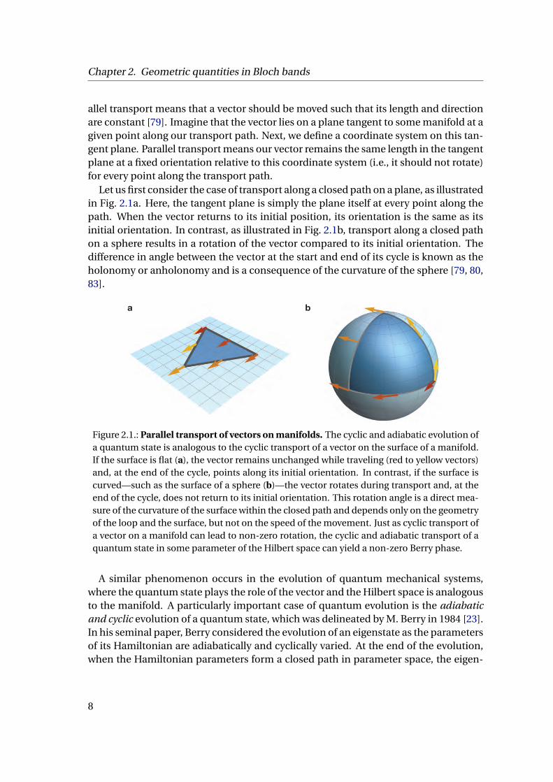
Let us first consider the case of transport along a closed path on a plane, as illustratedin Fig. 2.1a. Here, the tangent plane is simply the plane itself at every point along thepath. When the vector returns to its initial position, its orientation is the same as itsinitial orientation. In contrast, as illustrated in Fig. 2.1b, transport along a closed pathon a sphere results in a rotation of the vector compared to its initial orientation. Thedifference in angle between the vector at the start and end of its cycle is known as theholonomy or anholonomy and is a consequence of the curvature of the sphere [79, 80,83].
a b
Figure 2.1.: Parallel transport of vectors on manifolds. The cyclic and adiabatic evolution ofa quantum state is analogous to the cyclic transport of a vector on the surface of a manifold.If the surface is flat (a), the vector remains unchanged while traveling (red to yellow vectors)and, at the end of the cycle, points along its initial orientation. In contrast, if the surface iscurved—such as the surface of a sphere (b)—the vector rotates during transport and, at theend of the cycle, does not return to its initial orientation. This rotation angle is a direct mea-sure of the curvature of the surface within the closed path and depends only on the geometryof the loop and the surface, but not on the speed of the movement. Just as cyclic transport ofa vector on a manifold can lead to non-zero rotation, the cyclic and adiabatic transport of aquantum state in some parameter of the Hilbert space can yield a non-zero Berry phase.
A similar phenomenon occurs in the evolution of quantum mechanical systems,where the quantum state plays the role of the vector and the Hilbert space is analogousto the manifold. A particularly important case of quantum evolution is the adiabaticand cyclic evolution of a quantum state, which was delineated by M. Berry in 1984 [23].In his seminal paper, Berry considered the evolution of an eigenstate as the parametersof its Hamiltonian are adiabatically and cyclically varied. At the end of the evolution,when the Hamiltonian parameters form a closed path in parameter space, the eigen-
8
2.1. Geometric phases in brief
state returns to itself but has picked up a phase factor. This phase factor is comprisedof a dynamical part which depends on the time taken en-route, and a geometric partgiven by ∮
Ci ⟨Ψ|∇x|Ψ⟩ ·dx, (2.1)
where |Ψ⟩ is the state, ∇x takes partial derivatives with respect to the variable x, xparametrizes the change in the Hamiltonian, and the contour C forms a closed path inparameter space. Notably, this geometric phase, now commonly called Berry’s phase,depends only on the geometry of the path.
Returning to our example above, the Berry’s phase acquired in the cyclic evolutionof a quantum state in the Hilbert space is analogous to the holonomy acquired in thecyclic evolution of a vector on a manifold. Two important quantities associated withthe Berry phase are the Berry connection and the Berry curvature. The Berry connec-tion specifies the conditions for parallel transport of the quantum state [79], in analogyto our rules for parallel transport of the vector, i.e., that it does not change direction orlength. In Eq. 2.1, the Berry connection is the integrand. The Berry curvature, as itsname suggests, influences the Berry phase of the quantum state as the curvature of themanifold influences the holonomy of the vector. By Stokes’ theorem, the Berry curva-ture is curl of the Berry connection [84]. We shall later examine these terms in moredetail.
Since their inception, Berry’s ideas have found widespread applications in physicsand inspired a multitude of work [83]. A particularly important generalization ofBerry’s phase was made by Wilczek and Zee in 1984 when they considered adiabaticevolution in degenerate systems, where adiabatic now means that the evolution al-ways stays in the subspace of degenerate states [76]. In this case, the initial state istransformed by a matrix called the Wilson line, a term which originally comes from thefield of quantum chromodynamics [85]. In fact, in their paper, Wilczek and Zee werenot considering questions of band structures but rather noting the remarkable fact thatthe same mathematical structures arise in both the adiabatic evolution of simple quan-tum mechanical systems and the more complex gauge theories of fundamental inter-actions [76].
Since it is a matrix, the Wilson line can result in population changes between thedegenerate states, in contrast to Berry phases which result only in the acquisition of aphase factor. Furthermore, Wilson lines can be non-commuting. For example, imag-ine taking two closed paths in parameter space. When the evolution is described bythe Berry phase, the order in which the paths are taken does not matter because phasefactors always commute. However, if the evolution is in a degenerate system, the fi-nal state could differ depending on which closed path is first traversed. This non-commuting or non-abelian property is central to proposals on geometric quantumcomputing [86, 87].
9

Chapter 2. Geometric quantities in Bloch bands
Paralleling the relationship between the Berry phase and Berry connection, the Wil-son line is obtained by integrating a Berry connection matrix. Similar to the standardBerry connection, the Berry connection matrix specifies the rules for parallel trans-port, with the only difference being that the parallel transport now occurs in a morecomplex, degenerate subspace. Likewise, there is a quantity called the non-abelianBerry curvature that is analogous to the standard Berry curvature. However, in defin-ing it from the Berry connection matrix, the curl is replaced by the covariant deriva-tive [88]. Furthermore, in contrast to the standard, non-degenerate system, Stokes’theorem does not apply here, so there is no analogous formulation of the Wilson linein terms of the non-abelian Berry curvature [80]. In essence, there are related geomet-ric quantities in degenerate and non-degenerate systems. However, in the case of thelatter, the mathematics are often more involved and a physical picture less accessible.
2.2. Accessing geometric properties in Bloch bands
Having discussed geometric quantities arising from the evolution of general quantumsystems, we now turn our attention to the specific case of band structures. We beginthis section by defining some key quantities that will be used in calculating the equa-tions of motion for a single particle in a periodic potential subject to a constant externalforce. We will see that the equations of motion will contain both dynamical factors thatdepend on the time taken for the evolution and geometric factors that are determinedsolely by the band geometry. Furthermore, we examine the two limiting cases of a verysmall and a very large force and find that the unitary evolution operator is the Berryphase factor and the Wilson line, respectively.
2.2.1. Preliminaries
The solutions to the Schroedinger equation of a single-particle in a periodic potentialare given by the Bloch states Φn
q (r) and the energies E nq [1]. The index q is the quasi-
momentum or crystal momentum. Since the Brillouin zones are periodic, the quasi-momentum can always be confined to the first Brillouin zone. At every q, there are aninfinite number of discretely spaced eigenenergies, which are labeled with the bandindex n. From Bloch’s theorem, the Bloch state of band n at quasimomentum q can bewritten as:
Φnq (r) = e
iħq·run
q (r), (2.2)
where eiħq·r is a plane-wave and un
q (r) is called the cell-periodic Bloch function becauseit has the same periodicity as the potential. That is, if R is a direct lattice vector suchthat the potential V (r) =V (r+R), then un
q (r) = unq (r+R). For simplicity, we will hence-
10
2.2. Accessing geometric properties in Bloch bands
forth work in Dirac notation and set ħ= 1. In Dirac notation, the Bloch state is
|Φnq⟩ = e i q·r|un
q ⟩, (2.3)
where r is the position operator.1
When a constant force is applied to this periodic system, the quasimomentum be-comes time-dependent and the Bloch states are no longer the eigenstates of the (new)Hamiltonian [1]. For a force F, the quasimomentum evolves as [1, 89]:
q(t ) = q(0)+Ft . (2.4)
The quasimomentum is now the time-dependent parameter of the Hamiltonian, yield-ing a system analogous to the one originally considered by Berry. In our subsequentderivation, we will similarly see the Berry connection naturally arises in the equationsof motion.
In the Bloch bands, the Berry connection is defined by the cell-periodic Bloch func-tions as [26]:
An,n′q = i ⟨un
q |∇q|un′q ⟩. (2.5)
When n 6= n′, this quantity is often called the non-abelian Berry connection to distin-guish it from the standard Berry connection, where n = n′. The Berry phase, as definedin Eq. 2.1, is the line-integral of the standard Berry connection (where n = n′) in re-ciprocal space. There is no equivalent definition of a Berry phase for the non-abelianBerry conection. However, as we will later see, the non-abelian Berry connection ispart of the matrix-valued Wilson line.
1The equivalence of Eqs. 2.3 and 2.2 can be shown by projecting Eq. 2.2 into the position-basis:
⟨r|Φnq⟩ = ⟨r|e i q·r|un
q ⟩
= ⟨r|(i q · r+ (i q · r)2
2!+ ...)|un
q ⟩
= ⟨r|(i q · r+ (i q · r)2
2!+ ...)|un
q ⟩= ⟨r|e i q·r|un
q ⟩= e i q·r⟨r|un
q ⟩→Φn
q (r) = e i q·runq (r)
where we have expanded the exponential as (i q · r+ (i q·r)2
2! + ...) in the second line and used that thestate |r⟩ is an eigenstate of the position operator r as r|r⟩ = r|r⟩ in the third line. We put the powerseries back as an exponential in the fourth line and, in the fifth line, used that e i q·r commutes with⟨r|. This gives the Bloch state in Dirac notation projected onto the position-basis.
11
Chapter 2. Geometric quantities in Bloch bands
2.2.2. Derivation of the equations of motion
In the basis of the Bloch states, the Hamiltonian of the lattice is
H = ∑q,n
E nq |Φn
q⟩⟨Φnq |. (2.6)
where E nq is the energy of the nth band at quasimomentum q.
Adding a constant force F to the system results in a Schroedinger equation
i∂t |ψ(t )⟩ = (H −F · r)|ψ(t )⟩. (2.7)
We assume the initial state at t = 0 is localized in reciprocal space at quasimomentumq0 such that
|ψ(0)⟩ =∑nαn(0)|Φn
q0⟩ (2.8)
where |αn(0)|2 gives the population in the nth band at time t = 0. To solve Eq. 2.7, weexpress the time-evolved state |ψ(t )⟩ as a superposition of Bloch states:
|ψ(t )⟩ =∑nαn(t )|Φn
q(t )⟩ (2.9)
Substituting Eqs. 2.9 and the time-dependence of the quasimomentum (Eq. 2.4 withħ= 1) into Eq. 2.7 yields the following equation of motion for coefficient αn :
i∂tαn(t ) = E n
q(t )αn(t )−∑
n′An,n′
q(t ) ·F αn′(t ) (2.10)
where
An,n′q(t ) = i ⟨un
q |∇q|un′q ⟩|q=q(t ). (2.11)
This is precisely the Berry connection defined in Eq. 2.5. Therefore, from Eq. 2.10, we
see that the evolution depends on the energies E nq(t ) and the Berry connections An,n′
q(t ) .In the case of a single band, Eq. 2.5 reduces to an acquisition of the familiar dynamicaland Berry phase factors.
Although these equations apply to any number of bands, we will focus on two-bandsystems, which is the most relevant for the experiments in this thesis. For a two-bandsystem, the equations of motion in matrix-form are
i∂t
(α1(t )
α2(t )
)=
E 1q(t ) − A11
q(t ) ·F −A12q(t ) ·F
−A21q(t ) ·F E 2
q(t ) − A22q(t ) ·F
(α1(t )
α2(t )
)(2.12)
12
2.2. Accessing geometric properties in Bloch bands
Generally, Eq. 2.12 must be numerically solved. However, we can nonetheless gainsome intuition by examining some qualitative features. To this end, it is useful to em-ploy an analogy to the familiar quantum optics problem of a two-level atom in a laserfield. Recall that, after making the rotating-wave approximation, the diagonal termsspecify the detuning of the laser field to the atomic transition and the off-diagonal ele-ments give the Rabi frequency, which parametrizes the coupling strength between thetwo levels.
In our system, the time-dependent Rabi frequency is
−2A12q(t ) ·F. (2.13)
Hence, we see that the non-abelian Berry connection is responsible for interband tran-sitions. Similarly, the time-dependent detuning is
E 1q(t ) − A11
q(t ) ·F− (E 2q(t ) − A22
q(t ) ·F). (2.14)
Here, the dispersion and the standard Berry connections play the role of the detuning.
In the case of a two-level atom interacting with a light-field, if the detuning is muchlarger than the Rabi frequency, interband transitions are suppressed. Conversely, if theRabi frequency is much larger than the detuning, full population transfer can occur be-tween the ground and excited states. In our system, the "knob" for tuning the strengthof the Rabi frequency relative to the detuning is the magnitude of the force. Using avery small force enables us to neglect interband transitions, while using a very largeforce enables us to neglect the dispersion relation E n
q . Next, we more closely examinethese two limiting cases.
2.2.3. Adiabatic motion: the Berry phase
We define using a “very small force" to mean that the atoms move in the Bloch bandsbut do not make transitions to other bands, i.e., the motion is adiabatic. Hence, thefinal distribution of the atomic population at the end of the evolution will be identicalto that of the initial distribution of the atomic population. Consequently, the coeffi-cients of the Bloch states only pick up (individual) phase factors during the course ofthe evolution and Eq. 2.12 reduces to
i∂t
(α1(t )
α2(t )
)=
E 1q(t ) − A11
q(t ) ·F 0
0 E 2q(t ) − A22
q(t ) ·F
(α1(t )
α2(t )
)(2.15)
The unitary time-evolution operator governing the evolution of an initial state |ψ(0)⟩
13
Chapter 2. Geometric quantities in Bloch bands
Ener
gy
Wilson lineBerry phase degeneratelevels
W
qi qf qi qf
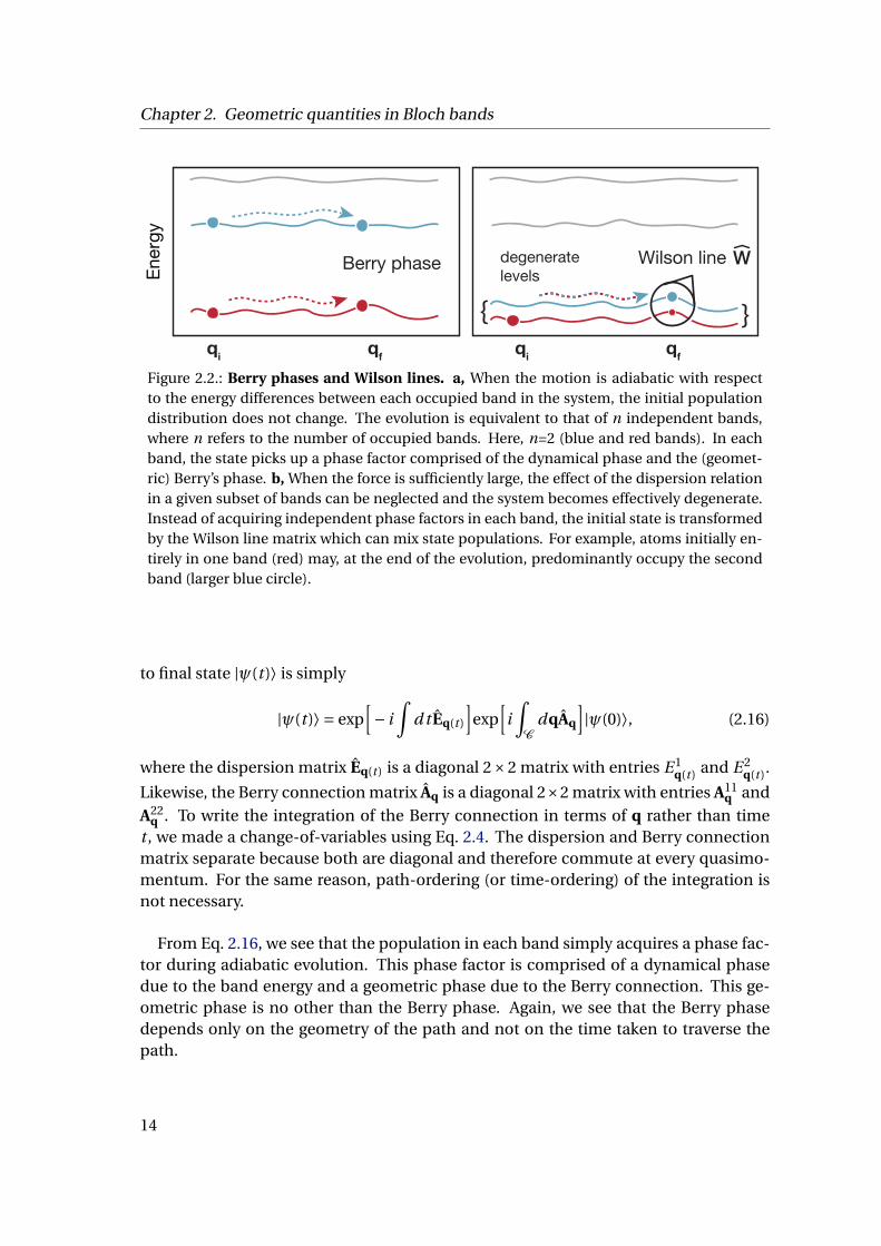
Figure 2.2.: Berry phases and Wilson lines. a, When the motion is adiabatic with respectto the energy differences between each occupied band in the system, the initial populationdistribution does not change. The evolution is equivalent to that of n independent bands,where n refers to the number of occupied bands. Here, n=2 (blue and red bands). In eachband, the state picks up a phase factor comprised of the dynamical phase and the (geomet-ric) Berry’s phase. b, When the force is sufficiently large, the effect of the dispersion relationin a given subset of bands can be neglected and the system becomes effectively degenerate.Instead of acquiring independent phase factors in each band, the initial state is transformedby the Wilson line matrix which can mix state populations. For example, atoms initially en-tirely in one band (red) may, at the end of the evolution, predominantly occupy the secondband (larger blue circle).
to final state |ψ(t )⟩ is simply
|ψ(t )⟩ = exp[− i
∫d t Eq(t )
]exp
[i∫C
dqAq
]|ψ(0)⟩, (2.16)
where the dispersion matrix Eq(t ) is a diagonal 2×2 matrix with entries E 1q(t ) and E 2
q(t ).
Likewise, the Berry connection matrix Aq is a diagonal 2×2 matrix with entries A11q and
A22q . To write the integration of the Berry connection in terms of q rather than time
t , we made a change-of-variables using Eq. 2.4. The dispersion and Berry connectionmatrix separate because both are diagonal and therefore commute at every quasimo-mentum. For the same reason, path-ordering (or time-ordering) of the integration isnot necessary.
From Eq. 2.16, we see that the population in each band simply acquires a phase fac-tor during adiabatic evolution. This phase factor is comprised of a dynamical phasedue to the band energy and a geometric phase due to the Berry connection. This ge-ometric phase is no other than the Berry phase. Again, we see that the Berry phasedepends only on the geometry of the path and not on the time taken to traverse thepath.
14
2.2. Accessing geometric properties in Bloch bands
2.2.4. Diabatic motion: the Wilson line
We define a “very large" force to mean that F is large enough such that the Berry con-
nection terms An,n′q(t ) ·F are much greater than the dispersion E n
q(t ). Neglecting the energyterm, Eq. 2.12 is
i∂t
(α1(t )
α2(t )
)=
−A11q(t ) ·F −A12
q(t ) ·F
−A21q(t ) ·F −A22
q(t ) ·F
(α1(t )
α2(t )
)(2.17)
Accordingly, the evolution of a state |ψ(0)⟩ to |ψ(t )⟩ is given by
|ψ(t )⟩ =T exp[
i∫
d t Aq(t ) ·F]|ψ(0)⟩
=Pexp[
i∫C
dqAq
]|ψ(0)⟩
≡ Wqi→q f |ψ(0)⟩ (2.18)
where C is the path taken from initial quasimomentum qi to the final quasimomen-tum q f , and P (T ) is the path (time)-ordering operator. In contrast to the adiabaticcase, path (time)-ordering is necessary because matrices Aq(q(t )), which are generallynot diagonal, may not commute at all integration points.
In contrast to the case of adiabatic evolution, which amounts to the independentacquisition of dynamical and geometric phase factors in each band, the unitary evolu-tion operator here is not diagonal and can therefore mix state populations. This matrixWqi→q f is called the Wilson loop or Wilson line, depending on whether the evolutionpath is a closed loop or an open line [85]. For generality, we shall most commonly usethe term Wilson line.
In our analysis, by neglecting the band energies, we effectively solved for the evolu-tion of a degenerate system. That is, by moving very fast in a non-degenerate system,we can reach a regime where the dynamics are equivalent to moving adiabatically in adegenerate system. Furthermore, in contrast to adiabatic evolution in the bands whichprobes both the dispersion and the Berry connection, the strong-gradient evolutionaccesses only the geometric quantities of the bands. As a concrete example, considera system containing only a single band. In this case, the Berry connection matrix hassize 1×1. Integrating this Berry connection “matrix" yields the standard Berry phaseof Sec. 2.2.3. Hence, Wilson lines are simply a generalization of the Berry phase factorto multiple, degenerate bands. In analogy, the eigenvalues of Wilson lines are knownas the non-abelian Berry phases [90].
15
Chapter 2. Geometric quantities in Bloch bands
2.3. Gauge invariance: which quantities are measurable?
In quantum mechanics, transforming a state |Ψ⟩ → |Ψ′⟩ = e iγ|Ψ⟩ by a phase factor istermed a gauge-transformation [81, 82]. Quantities that are not affected by this gauge-transformation are termed gauge-invariant. For example, the mean position ⟨Ψ|r|Ψ⟩of the state |Ψ⟩ is a gauge-invariant quantity because the gauge-transformed quantity⟨Ψ′|r|Ψ′⟩ is equivalent to the original quantity. In fact, physical observables are alwaysgauge-invariant, i.e., independent of basis choice.
In this section, we examine which geometric quantities are gauge-invariant andthereby measurable in the single- and multi-band case. Our analysis will show theimportance of taking closed paths in parameter space.
2.3.1. Single-band geometric quantities
We begin by checking if the standard Berry connections are gauge-invariant by makingthe gauge-transformation
|unq ⟩→ e iγn
q |unq ⟩ (2.19)
The Berry connection (n = n′) transforms as
An,nq → An,n
q +∇qγnq (2.20)
Our analysis shows that the Berry connection is not gauge-invariant and is thereforenot a measurable quantity.
Integrating the (standard) Berry connection over some path C in reciprocal spaceyields the Berry phase. Under the same transformation given in Eq. 2.19, the Berryphase transforms as: ∫
CdqAn,n
q →∫C
dq(An,nq +∇qγ
nq )
=∫C
dqAn,nq + (γn
q f−γn
qi), (2.21)
where q f and qi specify the final and initial points of the path C . Here, we see thatthe Berry phase is, in general, not gauge-invariant. However, for a closed path whereq f = qi , the term (γn
q f−γn
qi) = 0. Therefore, we see that for closed paths, the Berry phase
is indeed gauge-invariant and measurable.
Another way of formulating the Berry phase is to use Stokes’ theorem to relate theline-integral over a closed contour to an area integral [84]. Doing so gives an equivalent
16
2.3. Gauge invariance: which quantities are measurable?
expression of the Berry phase as∫C
dqAn,nq =
∫S
d 2q∇×An,nq (2.22)
where S is the surface enclosed by the path C = ∂S . The quantity
Ωnq =∇×An,n
q (2.23)
is called the Berry curvature and gauge-transforms as:
∇×An,nq →∇× (An,n
q +∇qγnq ) =∇×An,n
q (2.24)
Hence, the Berry curvature is gauge-invariant and therefore measurable. Since theBerry phase can be formulated in terms of an area integral, it is also sometimes calledthe Berry flux.
The gauge-invariance of the Berry curvature is particularly useful when we actuallywant to compute the Berry phase. This is because calculating the Berry connection re-quires the cell-periodic Bloch functions to be smooth and continuous because we needto take derivatives. However, numerical calculations generally assign random phasefactors to each cell-periodic Bloch function. Although there are some prescriptionson how to then modify the gauge to obtain differentiable cell-periodic Bloch func-tions [91], it is often easier to avoid this gauge-choice issue altogether and use the Berrycurvature to calculate the Berry phase [26].
2.3.2. Multi-band geometric quantities
Before examining the matrix-valued quantities, we first take a look at the non-abelian
Berry connection An,n′q , where n 6= n′. Although the (standard) Berry connection of a
single band was gauge-dependent, under the same gauge-transformation of Eq. 2.19,the non-abelian Berry connection becomes
An,n′q → e i (γn
q−γn′q )An,n′
q for n 6= n′ (2.25)
Since it is transformed only by a phase factor, the absolute value of the non-abelianBerry connection is gauge-invariant and therefore a physical observable. Recall in thediscussion near the end of Sec. 2.2.2 that the non-abelian Berry connection is respon-sible for coupling the bands. Therefore, the absolute value of the non-abelian Berryconnection corresponds to a Rabi frequency, which we will later measure in Sec. 7.1.1.
When writing a state in terms of n basis states, the system has U (n) gauge-freedom.For example, in the single-band case, we had U (1) gauge-freedom, meaning that wewere able to change the state by an arbitrary phase-factor. In the multi-band case, the
17

Chapter 2. Geometric quantities in Bloch bands
state |Ψq⟩ =(α1
q
α2q
)written in the basis of the Bloch states of the first and second band at
quasimomentum q transforms as
|Ψq⟩→ Uq|Ψq⟩, (2.26)
where Uq is a quasimomentum-dependent U (2) matrix.Under such a gauge-transformation, the Berry connection matrix Aq becomes
Aq → UqAqU †q − i (∇qUq)U †
q. (2.27)
Just like the standard Berry connection, the Berry connection matrix is gauge-dependent.
The Wilson line transforms as
Wqi→q f → Uq f Wqi→q f U †qi
(2.28)
and is also gauge-dependent. However, in analogy with the Berry phase, the eigen-values of a Wilson loop, i.e., the Wilson line of a closed path, are gauge-invariant. If astate |Ψqi ⟩ is an eigenstate of the Wilson line operator Wqi→q f with eigenvalue λ, thena gauge transformation yields:
W′qi→q f
|Ψ′qi⟩ = Uq f Wqi→q f U †
qiUqi |Ψqi ⟩
= Uq f λ|Ψqi ⟩=λ|Ψ′
qi⟩ if q f = qi (2.29)
The eigenvalues of a Wilson loop are often called the non-abelian Berry phases.Finally, for completeness, we note that the non-abelian Berry curvature is defined
as [26]
Fq =∇×Aq − i Aq ×Aq (2.30)
and gauge transforms as
Fq → UqFqU †q (2.31)
Unlike the standard Berry curvature, the non-abelian Berry curvature is not gauge-invariant and therefore not an observable quantity.
2.3.3. A summary
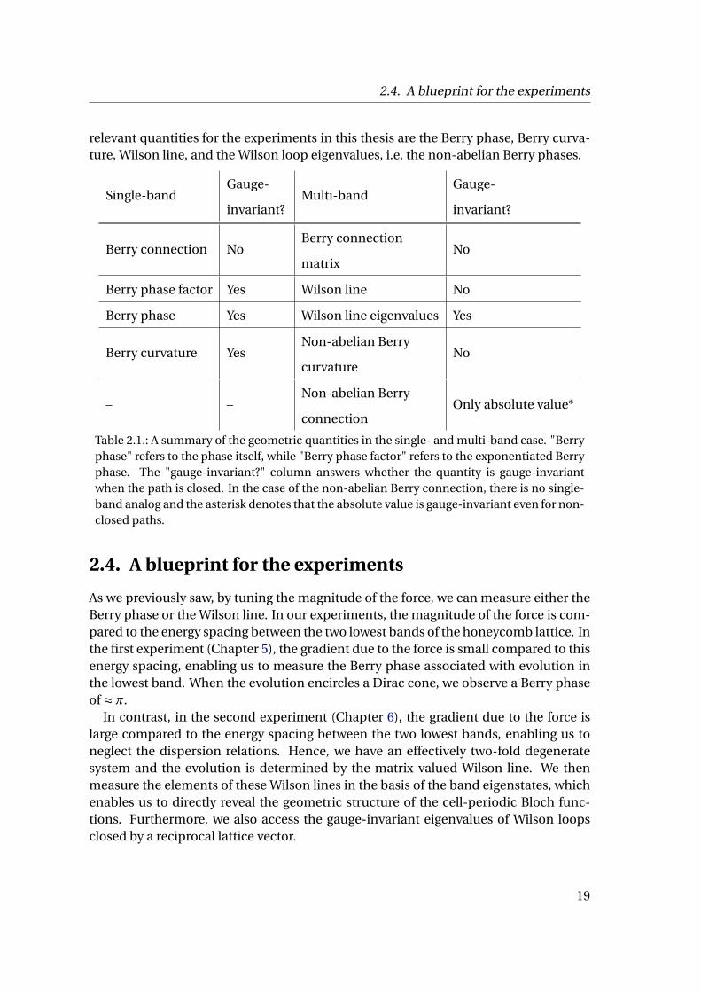
We summarize the results of our gauge-invariance discussion in Table 2.1, wheregauge-invariant quantities for a closed loop are denoted with an asterisk.. The most
18
2.4. A blueprint for the experiments
relevant quantities for the experiments in this thesis are the Berry phase, Berry curva-ture, Wilson line, and the Wilson loop eigenvalues, i.e, the non-abelian Berry phases.
Single-bandGauge-
invariant?Multi-band
Gauge-
invariant?
Berry connection NoBerry connection
matrixNo
Berry phase factor Yes Wilson line No
Berry phase Yes Wilson line eigenvalues Yes
Berry curvature YesNon-abelian Berry
curvatureNo
– –Non-abelian Berry
connectionOnly absolute value*
Table 2.1.: A summary of the geometric quantities in the single- and multi-band case. "Berryphase" refers to the phase itself, while "Berry phase factor" refers to the exponentiated Berryphase. The "gauge-invariant?" column answers whether the quantity is gauge-invariantwhen the path is closed. In the case of the non-abelian Berry connection, there is no single-band analog and the asterisk denotes that the absolute value is gauge-invariant even for non-closed paths.
2.4. A blueprint for the experiments
As we previously saw, by tuning the magnitude of the force, we can measure either theBerry phase or the Wilson line. In our experiments, the magnitude of the force is com-pared to the energy spacing between the two lowest bands of the honeycomb lattice. Inthe first experiment (Chapter 5), the gradient due to the force is small compared to thisenergy spacing, enabling us to measure the Berry phase associated with evolution inthe lowest band. When the evolution encircles a Dirac cone, we observe a Berry phaseof ≈π.
In contrast, in the second experiment (Chapter 6), the gradient due to the force islarge compared to the energy spacing between the two lowest bands, enabling us toneglect the dispersion relations. Hence, we have an effectively two-fold degeneratesystem and the evolution is determined by the matrix-valued Wilson line. We thenmeasure the elements of these Wilson lines in the basis of the band eigenstates, whichenables us to directly reveal the geometric structure of the cell-periodic Bloch func-tions. Furthermore, we also access the gauge-invariant eigenvalues of Wilson loopsclosed by a reciprocal lattice vector.
19
Chapter 2. Geometric quantities in Bloch bands
For both experiments, the three main ingredients required are similar. We must2:
1. Prepare a quantum state at an initial quasimomentum qi : |Ψqi ⟩2. Evolve the state to final quasimomentum q f : Wqi→q f |Ψqi ⟩
3. Detect the new state Wqi→q f |Ψqi ⟩These three ingredients are readily available in our cold-atom toolbox and detailed
in our discussion of the experimental setup in Chapter 4. First, in the next chapter, weintroduce the honeycomb lattice and examine its geometric attributes.
2 Here, we have used the Wilson line as the evolution operator for generality. Recall that in the case ofa single band, the Wilson line is simply the Berry phase factor.
20
Chapter 3.
The optical honeycomb lattice
We begin this chapter by deriving the single-particle tight-binding model for the hon-eycomb lattice, which contains two sites, A and B, in its unit cell. We examine thedispersion and eigenstates when A and B sites are degenerate and find a degeneracy inthe energy spectrum (sec. 3.1.1). In the vicinity of this degeneracy, the dispersion is lin-ear and resembles that of the massless Dirac equation. Appropriately, this degeneracypoint is called the Dirac point. We show that taking even an infinitesimal loop aroundthe Dirac point yields a Berry phase of π.
Next, we consider the dispersion and eigenstates when there is an energy offset be-tween A and B sites (sec. 3.1.2). To more conveniently analyze the scenario, we intro-duce the Bloch sphere picture, where the evolution of an eigenstate in reciprocal spaceis visualized as a rotation of a vector of unit length. We illustrate the difference betweenevolutions in a lattice with degenerate and non-degenerate A and B sites. Furthermore,we show that paths that encircle a Dirac point enclose a non-zero solid angle on theBloch sphere. We derive the relation between this solid angle and the Berry phase.
In the second part of this chapter, we introduce an ab-initio single-particle calcu-lation for the optical honeycomb potential (Sec. 3.2). We compare the ab-initio andtight-binding dispersions and find that, although a minimum lattice depth is requiredbefore the ab-initio dispersion begins to closely resemble the tight-binding dispersion,the Dirac points are always present even at very low lattice depths (Sec. 3.2.3). Lastly,in order to better understand the appearance of multiple sets of bands in the ab-initiocalculation, we consider the limiting cases of a vanishing and very deep lattice, wherethe system is that of a free-particle and a harmonic oscillator, respectively.
3.1. The tight-binding model
The honeycomb lattice is not a monoatomic Bravais lattice, but rather a Bravais latticewith a two-site unit cell. It can be decomposed into two triangular sublattices com-posed of A and B sites (see Fig. 3.1a). The primitive direct lattice vectors spanning the
21
Chapter 3. The optical honeycomb lattice
a
a1
a2
a
δ1
δ2
δ3
b
kL
A B
M
K
K’
Γ
x
y
qx
qy
b1
b2
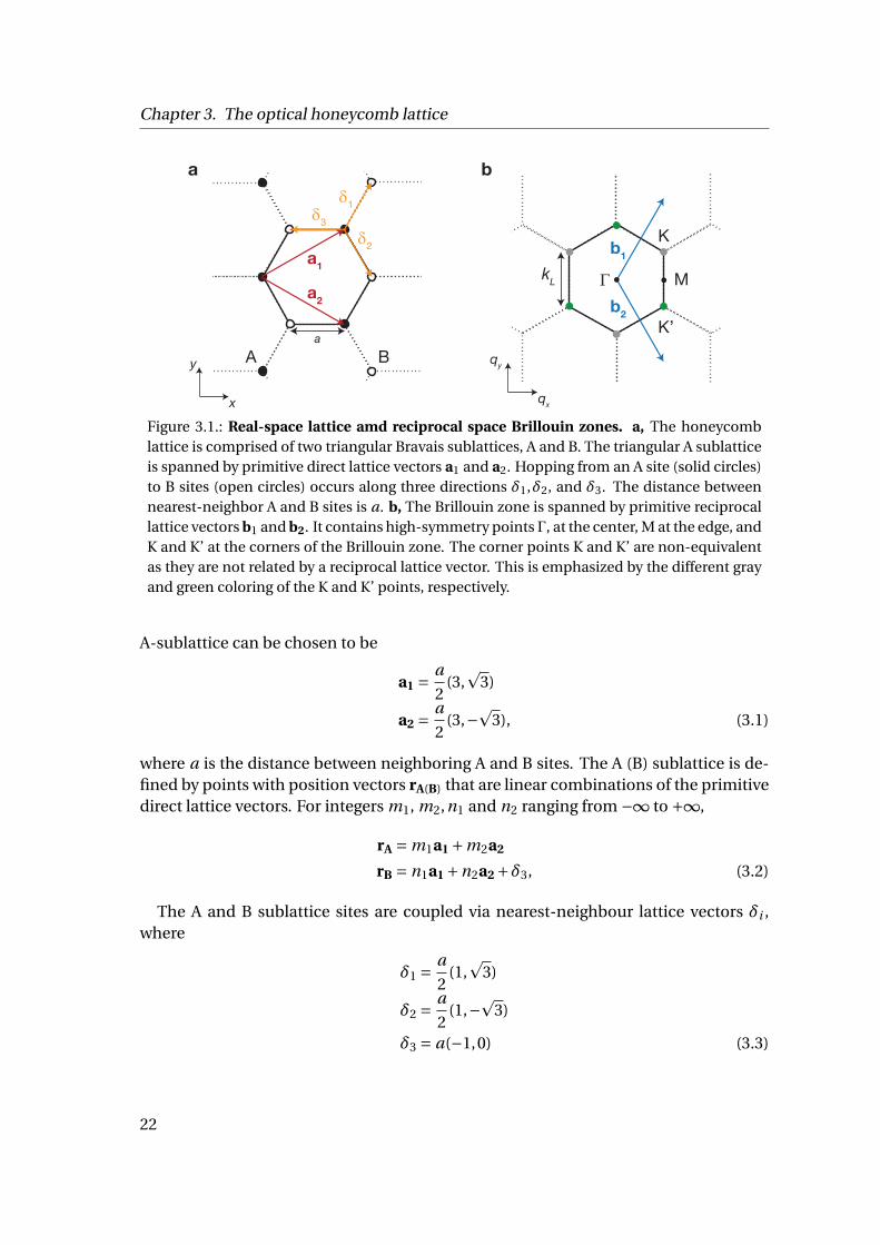
Figure 3.1.: Real-space lattice amd reciprocal space Brillouin zones. a, The honeycomblattice is comprised of two triangular Bravais sublattices, A and B. The triangular A sublatticeis spanned by primitive direct lattice vectors a1 and a2. Hopping from an A site (solid circles)to B sites (open circles) occurs along three directions δ1,δ2, and δ3. The distance betweennearest-neighbor A and B sites is a. b, The Brillouin zone is spanned by primitive reciprocallattice vectors b1 and b2. It contains high-symmetry pointsΓ, at the center, M at the edge, andK and K’ at the corners of the Brillouin zone. The corner points K and K’ are non-equivalentas they are not related by a reciprocal lattice vector. This is emphasized by the different grayand green coloring of the K and K’ points, respectively.
A-sublattice can be chosen to be
a1 = a
2(3,
p3)
a2 = a
2(3,−p3), (3.1)
where a is the distance between neighboring A and B sites. The A (B) sublattice is de-fined by points with position vectors rA(B) that are linear combinations of the primitivedirect lattice vectors. For integers m1, m2,n1 and n2 ranging from −∞ to +∞,
rA = m1a1 +m2a2
rB = n1a1 +n2a2 +δ3, (3.2)
The A and B sublattice sites are coupled via nearest-neighbour lattice vectors δi ,where
δ1 = a
2(1,
p3)
δ2 = a
2(1,−p3)
δ3 = a(−1,0) (3.3)
22
3.1. The tight-binding model
Associated with the real-space lattice is a reciprocal lattice. The primitive reciprocallattice vectors bi (i = 1,2) that fulfill the condition ai ·bi = 2πδi j [1], where δi j is theKronecker delta, are
b1 = 2π
3a(1,
p3) = kL(
p3
2,
3
2)
b2 = 2π
3a(1,−p3) = kL(
p3
2,−3
2), (3.4)
where we have defined kL = 4π3p
3a.
The reciprocal lattice, like the direct lattice, has a honeycomb structure. High-symmetry points Γ, located at the center of the Brillouin zone, M, located at the edge ofthe Brillouin zone, and K (K’), located at the corners of the Brillouin zone are illustratedin Fig. 3.1b. We emphasize that points K and K’ are inequivalent, as a K point cannot bereached from a K’ point by a reciprocal lattice vector. The importance of these points,known as Dirac points, will become apparent in the next sections.
The single-particle Hamiltonian describing nearest-neighbor hopping between Aand B sites with hopping amplitude J and an energy difference ∆ between A and Bsites can be written as
Htb =− J∑
⟨RB ,RA⟩|wRB ⟩⟨wRA |+ c.c
+ ∆2
∑⟨RA ,RA⟩
(|wRA⟩⟨wRA |− |wRB ⟩⟨wRB |), (3.5)
where |wRA(B)⟩ are the Wannier states localized on the A (B) sites.
Furthermore, in analogy to the Bloch states, we define quasimomentum-dependentstates |ΦA(B)
q ⟩ of the A (B) sites as
|ΦAq ⟩ =
1pN
∑rA
e i q·rA |wrA⟩ = e i q·r|u Aq ⟩ (3.6)
|ΦBq ⟩ =
1pN
∑rB
e i q·rB |wrB ⟩ = e i q·r|uBq ⟩, (3.7)
where N denotes the number of lattice sites and |u A (B)q ⟩ are the analogous cell-periodic
Bloch functions of the A (B) sites.
In the basis of |ΦAq ⟩ and |ΦB
q ⟩, the Hamiltonian describing the two lowest bands ofthe honeycomb lattice is
H tbq =
∆/2 tq
t∗q −∆/2
, (3.8)
23
Chapter 3. The optical honeycomb lattice
where
tq = ∣∣tq∣∣e iϑq = J
3∑i=1
e−i q·δi (3.9)
This Hamiltonian is diagonalized by eigenstates
|Φ1(2)q ⟩ = 1√∣∣∣ f 1(2)
q
∣∣∣2 +1
(f 1(2)
q e iϑq |ΦAq ⟩− |ΦB
q ⟩), (3.10)
where f 1(2)q = ∆−(+)
√∆2+4|tq|2
2|tq| .
The corresponding eigenenergies are
E 1(2)q =
−(+)√∆2 +4
∣∣tq∣∣2
2. (3.11)
3.1.1. ∆= 0: Dirac points and Berry phases
When ∆= 0, f 1(2)q =−(+)1 and the expression of the eigenstates in Eq. 3.10 reduces to
|Φ1(2)q ⟩ = 1p
2
(− (+)e iϑq |ΦA
q ⟩− |ΦBq ⟩
). (3.12)
That is, when the A and B sites are at the same energy, the eigenstates are in an equalsuperposition of the Bloch states of the A and B sites at every quasimomentum. UsingEq. 3.12, the standard Berry connections of the first and second band are
A11q = A22
q = 1
2∇qϑq (3.13)
and the off-diagonal or non-Abelian Berry connections are
A12q = A21
q =−1
2∇qϑq (3.14)
The dispersion (see Fig. 3.2a) at Γ ≡ (qx = 0, qy = 0) has an energy gap of 6J . AtM≡ kL(qx = p
3/2, qy = 0), the gap is 2J . At K≡ kL(qx = p3/2, qy = 1/2), however,
the bands are degenerate. Furthermore, in the vicinity of the K point, the dispersionlooks linear. To quantitatively examine the behavior of the dispersion and eigenstatesin the vicinity of the K point, we expand in q at quasimomentum K−q. This yields a
24
3.1. The tight-binding model
Hamiltonian
H Kq = νF
0 qx + i qy
qx − i qy 0
= νF∣∣q∣∣ 0 e iφ
e−iφ 0
, (3.15)
whereνF = 3Ja/2. In the second equality, we have expressed the matrix in polar coordi-nates such that q = ∣∣q∣∣e iφ. This change of coordinates enables us to more convenientlyanalyze the problem.
The eigenenergies are
±νF∣∣q∣∣ . (3.16)
Here, we see that the eigenenergies are indeed linear in the distance∣∣q∣∣ to the K point.
This dispersion resembles the massless Dirac equation, for which the K point is named,with the exception that the speed of light is replaced by νF , commonly refered to asthe Fermi velocity. In material graphene, where νF is about 300 times smaller than thespeed of light, this linear dispersion relation results in novel transport phenomena thatare of great interest both fundamentally and for technological applications [75, 92].
Next, we examine the Berry phase acquired by a particle traversing an infinitesimalloop around the Dirac point in the lowest band. Doing so requires the cell-periodicpart of the eigenvectors of the Hamiltonian, which, expressed in the basis of |u A
q ⟩ and
|uBq ⟩, are
|u1(2)φ ⟩ = 1p
2
(−(+)e iφ
1
). (3.17)
In polar coordinates, the Berry connection of the lowest band is
A11q = i ⟨u1
q|∇q|u1q⟩→
(i ⟨u1
φ|∂|q||u1φ⟩, i
∣∣q∣∣⟨u1φ|∂φ|u1
φ⟩), (3.18)
where we have split the Berry connection into its∣∣q∣∣ and φ components. There is no
dependence of∣∣q∣∣ in the eigenstate, so the
∣∣q∣∣ component is zero. Theφ component is
A11φ = 1
2∣∣q∣∣ (3.19)
The Berry phase can then be expressed as∫C
A11q dq =
∫ 2π
0A11φ
∣∣q∣∣dφ=∫ 2π
0
1
2dφ=π, (3.20)
where C refers to the closed loop around the K point. Therefore, an infinitesimal loop
25

Chapter 3. The optical honeycomb lattice
a
Γ ΓM K
3
2
1
0
-3
-2
-1
E q/J
q
∆/J=0∆/J=0.5∆/J=1∆/J=1.5∆/J=2
1
M KK’
b
q
∆/J=0.1∆/J=0.2∆/J=0.3∆/J=0.4
K’
K
q1
Figure 3.2.: The tight-binding dispersion and Berry curvature with varying Semenoff mass.a, The dispersion along the high-symmetry path Γ-M-K-Γ for hopping strength J = 1. WhenA and B sites are degenerate (∆ = 0), there is a Dirac point at the K (and K’) point. At finiteenergy offset between A and B sites, an energy gap opens at the K (and K’) point, breakingthe degeneracy between the first and second bands. This energy gap increases as the en-ergy offset between A and B sites increases. b, The Berry curvature Ω1
q of the first band atK and K’ points for increasing values of ∆ (decreasing shades of red). As the Semenoff massis increased, the HWHM of the Berry curvature increases. In the massless case, the Berrycurvature is a delta function [93, 94].
around the K point results in a Berry phase (or flux) of π. The same analysis holdsfor the other two K points (at kL(0, − 1) and kL(−p3/2, 1/2)). Performing the samecalculation around K’ points (located at kL(0, 1), kL(
p3/2, −1/2), or kL(−p3/2, −1/2))
results in a Berry phase of −π. Hence, when ∆ = 0, we cannot distinguish betweenencircling the K or K’ point—both yield a phase of π=−π. In contrast, we will later seethat these two scenarios are distinguishable when ∆ 6= 0.
3.1.2. ∆ 6= 0: Effect of the Semenoff mass and the Bloch sphere picture
We now examine what happens when there is an energy offset between A and B sub-lattice sites. Introducing this energy offset is commonly called adding a Semenoffmass [95]. We see from Eqs. 3.11 and 3.10 that the Semenoff mass influences the formof both the eigenstates and the eigenergies. At the Dirac point, for example, the energydifference between the two bands is given by ∆. Hence, the larger the Semenoff mass,the larger the energy splitting at the Dirac points, as illustrated in Fig. 3.2a.
In terms of the eigenstates, the Semenoff mass imbalances their composition of Aand B sites. When ∆ = 0, the eigenstate at every quasimomentum is an equal super-position of the A and B site states. In contrast, when ∆ is non-zero, the A and B sitecomposition of the eigenstates becomes dependent on the quasimomentum, sign of∆, and the band. For example, let us specifically consider the lowest eigenstates. When
26
3.1. The tight-binding model
A and B sites are at the same energy, atoms favor both sites equally. In contrast, whenthere is an energy offset such that, for example, A sites are lower in energy than B sites,atoms will be preferentially located on A sites.
To visualize this effect, it is convenient to examine the eigenstates on a Bloch sphere,where the north and south poles are |u A
q ⟩ and |uBq ⟩, respectively, as shown in Fig. 3.3.
For simplicity, we shall draw only the eigenstate of the lower band.1 In it’s most generalform, the lower eigenstate at quasimomentum q is
|u1q⟩ = cos
θq
2e iϕq |u A
q ⟩+ sinθq
2|uB
q ⟩, (3.21)
where θq parametrizes the composition of andϕq parametrizes the phase between theA and B site states2.
For ∆= 0, the eigenstate is constrained along the equatorial plane at θq = π/2 as anequal superposition of A and B site states for every quasimomentum q. The rotationof the eigenstate for two closed paths, one around the Γ point and the other around aDirac cone, is shown Fig. 3.3. In contrast, the rotation of the eigenstate for ∆ = J forthe same two paths occurs in lower hemisphere. Since the A sites are at energy ∆/2while the B sites are at energy −∆/2, the eigenstate is now mostly comprised of the Bsite states.
Acquired Berry phase as the enclosed solid angle
Lastly, we highlight the difference between paths that enclose and do not enclose aDirac cone. In the former case, the evolution of the eigenstate encloses a solid angleon the Bloch sphere, while in the latter case, it does not (see Fig. 3.3). This is directly re-lated to whether the state acquires a non-trivial Berry phase along its evolution path. Inmore suggestive language, it is directly related to whether the evolution path enclosessome Berry flux, which requires a non-zero area element.
To understand this link, we first write down the solid angle subtended by a surfacein spherical coordinates, where r , θ, and ϕ parametrize the distance to the origin, thepolar angle, and the azimuthal angle, respectively:
S =∫
dS =∫ ∫
sinθdθdϕ. (3.22)
In our case, the relevant surface is the surface of the Bloch sphere enclosed by the evo-
1 Since the eigenstates of the lower and upper band are orthogonal, their orientations are not indepen-dent. Namely, if the eigenstate of the lower band has coordinates (ϕ,θ), where ϕ is the azimuthalangle and θ is the polar angle, the eigenstate of the upper band has coordinates (ϕ+π,π−θ). That is,they point in opposite direction on the Bloch sphere.
2 Note that the Bloch sphere representation neglects global phases. That is, we can not distinguish |u1q⟩
from e iγ|u1q⟩, where γ is a constant.
27
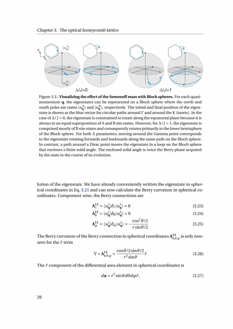
Chapter 3. The optical honeycomb lattice
∆/J=0 ∆/J=1
qx
qy
Figure 3.3.: Visualizing the effect of the Semenoff mass with Bloch spheres. For each quasi-momentum q, the eigenstates can be represented on a Bloch sphere where the north andsouth poles are states |u A
q ⟩ and |uBq ⟩, respectively. The initial and final position of the eigen-
state is shown as the blue vector for circular paths around Γ and around the K (insets). In thecase of∆/J = 0, the eigenstate is constrained to rotate along the equatorial plane because it isalways in an equal superposition of A and B site states. However, for∆/J = 1, the eigenstate iscomprised mostly of B site states and consequently rotates primarily in the lower hemisphereof the Bloch sphere. For both ∆ parameters, moving around the Gamma point correspondsto the eigenstate rotating forwards and backwards along the same path on the Bloch sphere.In contrast, a path around a Dirac point moves the eigenstate in a loop on the Bloch spherethat encloses a finite solid angle. The enclosed solid angle is twice the Berry phase acquiredby the state in the course of its evolution.
lution of the eigenstate. We have already conveniently written the eigenstate in spher-ical coordinates in Eq. 3.21 and can now calculate the Berry curvature in spherical co-ordinates. Component-wise, the Berry connections are
A11r = ⟨u1
q|∂r |u1q⟩ = 0 (3.23)
A11θ = ⟨u1
q|∂θ|u1q⟩ = 0 (3.24)
A11ϕ = ⟨u1
q|∂ϕ|u1q⟩ =−cos2θ/2
r sinθ/2(3.25)
The Berry curvature of the Berry connection in spherical coordinates A11r,θ,ϕ is only non-
zero for the r term
∇×A11r,θ,ϕ = cosθ/2sinθ/2
r 2 sinθr (3.26)
The r component of the differential area element in spherical coordinates is
da = r 2 sinθdθdϕr , (3.27)
28
3.1. The tight-binding model
giving
∇×A11r,θ,ϕ ·da =1
2sinθdθdϕ
= 1
2dS , (3.28)
where we have related the Berry curvature in a differential area to the solid angle fromEq. 3.22. Performing an area integral of the Berry curvature for the Berry phase gives
φBerry =∫
∇×A11r,θ,ϕda
= 1
2
∫ ∫sinθdθdϕ
= 1
2S (3.29)
We find that the Berry phase a state acquires is simply half of the solid-angle en-closed by the evolution of the state on the Bloch sphere. From this, we can imme-diately conclude that only the path enclosing a Dirac point yields a non-trivial Berryphase. Moreover, the π Berry phase that we analytically worked out in Sec. 3.1.1 can beunderstood here as resulting from a path that encloses half of the Bloch sphere (sincethe eigenstate is constrained on the equatorial plane). The solid angle of half a sphereis 2π, yielding a Berry phase of π.
In the presence of a Semenoff mass, the winding of the eigenstate is displaced fromthe equatorial plane. Consequently, the acquired Berry phase will be less than π, duethe decreased enclosure of solid angle. Moreover, if we acquire a phase of φBerry (thatis less than π) when encircling a K point, we will acquire a phase of −φBerry when en-circling a K’ point. Hence, in contrast to the massless (∆= 0) case, we would indeed beable to distinguish between encircling a K or K’ point. Visualized on the Bloch sphere,the eigenstates in these two scenarios would wind along the same path but in oppositedirections. For example, in Fig. 3.3, the eigenstate currently winds clockwise when en-circling a K point. When encircling a K’ point, it would instead wind counter-clockwise.
Lastly, as another way of understanding the effect of the Semenoff mass on the ac-quired Berry phase, we plot the Berry curvature of the first band as a function of quasi-momentum in Fig. 3.2b. When ∆ = 0, the Berry curvature is a delta function localizedat the K and K’ points [93, 94]. As ∆ is increased, the Berry curvature "spreads out" inthe sense that its half-width-half-max (HWHM) increases. Therefore, the Berry phaseacquired by encircling a K or K’ point decreases with increasing∆, due to the decreasedBerry flux in the enclosed area of the path. Furthermore, the opposite signs of the Berrycurvature at K and K’ yields Berry phases with opposite signs; this was previously un-derstood in the Bloch sphere picture as opposite winding directions of the eigenstates.The sign of the Berry curvature at the K and K’ points is determined by the symmetries
29
Chapter 3. The optical honeycomb lattice
of the Hamiltonian and has important implications for the topological character of thebands [22]. For example, since the Berry curvature at the K and K’ points have oppo-site sign in our case, we know that the Chern number, which is given by the integral ofthe Berry curvature over the whole Brillouin zone [8, 26], must be zero. Correspond-ingly, in, for example, the Haldane model, where the Chern number is finite, the Berrycurvature at K and K’ have the same sign.
3.2. The ab-initio calculation
Having derived a tight-binding model of the honeycomb lattice, we now provide an ab-initio calculation for a single particle confined in an optical honeycomb potential. Thisis necessary for the comparison of our actual experimental parameters to the tight-binding model.
3.2.1. Setting up the problem
We begin by writing down the Schroedinger equation of a single particle in a periodicpotential in the position basis:
HΨnq (r) =
( p2
2m+V (r)
)Ψn
q (r) = E nqΨ
nq (r), (3.30)
where p =−iħ∇ is the momentum operator and the potential V (r) is periodic such thatV (r+R) =V (r) for all Bravais lattice vectors R. This is a canonical problem in solid statetheory and can be found in any introductory solid state book (see e.g, Ref. [1]). FromBloch’s theorem, we know the Bloch functionsΨn
q (r) are plane waves multiplied by thecell-periodic Bloch functions which have the same periodicity as the potential:
Ψnq (r) = e
iħq·run
q (r). (3.31)
Substituting Eq. 3.31 into Eq. 3.30 yields an eigenvalue equation for the cell-periodicfunctions un
q (r):
HB unq (r) =
( (p+q)2
2m+V (r)
)un
q (r) = E nq un
q (r) (3.32)
Our goal now is to find the elements of the Hamiltonian HB such that we can numeri-cally diagonalize HB to obtain E n
q and unq (r). To this end, we expand un
q (r) in the planewave basis. Since un
q (r) has the same periodicity of the lattice, its plane wave expan-sion also contains only plane waves with the same periodicity of the lattice, i.e., its
30
3.2. The ab-initio calculation
plane wave expansion is comprised of the reciprocal lattice vectors K:
unq (r) =∑
Kc(n,q)
K e i K·r, (3.33)
where summation over K is to be understood as running over all reciprocal lattice vec-tors. Similarly, the potential V (r) can also be expanded as plane waves of the reciprocallattice vectors
V (r) =∑K′
VK′e i K′·r (3.34)
Substituting the plane wave expansions of Eq. 3.33 and Eq. 3.34 into Eq. 3.32 yields
∑K
((q+K)2
2mc(n,q)
K e i K·r +∑K′
VK′c(n,q)K e i (K+K′)·r = E n
q c(n,q)K e i K·r
)(3.35)
To select a particular plane wave coefficient c(n,q)K
with momentum K, we multiply both
sides of the equation by Ce−i K·r and integrate over all space, where C is a constant cho-sen to appropriately cancel out pre-factors in the integration. The resulting equationcan be written in matrix form as∑
KHKKc(n,q)
K = E nq c(n,q)
K(3.36)
where we have evaluated the Kronecker delta on the right-hand-side and
HKK = (q+K)2
2mδK,K +∑
K′VK′δK+K′,K (3.37)
3.2.2. Application to the optical honeycomb potential
Thus far, our analysis has been generic and applicable to any periodic potential. Toproceed further, we need to substitute in the reciprocal lattice vectors of the honey-comb potential. Although we already know what these vectors are from our tight-binding analysis, we would like to determine them using basic information on thesetup of the honeycomb optical lattice in the lab. Details on the experimental realiza-tion of the optical lattice are in Sec. 4.1; for now, we need only to know that the latticeis created by interfering three running-wave laser beams at 120 angles, as depicted in
31
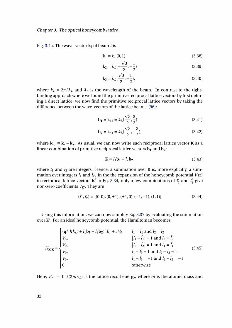
Chapter 3. The optical honeycomb lattice
Fig. 3.4a. The wave-vector ki of beam i is
k1 = kL(0,1) (3.38)
k2 = kL(−p
3
2,−1
2) (3.39)
k3 = kL(
p3
2,−1
2), (3.40)
where kL = 2π/λL and λL is the wavelength of the beam. In contrast to the tight-binding approach where we found the primitive reciprocal lattice vectors by first defin-ing a direct lattice, we now find the primitive reciprocal lattice vectors by taking thedifference between the wave-vectors of the lattice beams [96]:
b1 = k12 = kL(
p3
2,
3
2) (3.41)
b2 = k31 = kL(
p3
2,−3
2), (3.42)
where ki j ≡ ki −k j . As usual, we can now write each reciprocal lattice vector K as alinear combination of primitive reciprocal lattice vectors b1 and b2:
K = l1b1 + l2b2, (3.43)
where l1 and l2 are integers. Hence, a summation over K is, more explicitly, a sum-mation over integers l1 and l2. In the the expansion of the honeycomb potential V (r)in reciprocal lattice vectors K′ in Eq. 3.34, only a few combinations of l ′1 and l ′2 givenon-zero coefficients VK′ . They are
(l ′1, l ′2) = (0,0), (0,±1), (±1,0), (−1,−1), (1,1) (3.44)
Using this information, we can now simplify Eq. 3.37 by evaluating the summationover K′. For an ideal honeycomb potential, the Hamiltonian becomes
HK,K =
(q/(ħkL)+ l1b1 + l2b2)2Er +3V0, l1 = l1 and l2 = l2
V0,∣∣l1 − l1
∣∣= 1 and l2 = l2
V0,∣∣l2 − l2
∣∣= 1 and l1 = l1
V0, l1 − l1 = 1 and l2 − l2 = 1
V0, l1 − l1 =−1 and l2 − l2 =−1
0, otherwise
(3.45)
Here, Er = h2/(2mλL) is the lattice recoil energy, where m is the atomic mass and
32

3.2. The ab-initio calculation
a b c
E q/E
rn
0
2
4
6
8
10
12
Γ ΓM Kq
Γ ΓM Kq
E qn
k1
k2k3 v0=0.5Er
v0=2Er
v0=6Er
v0=10Er
tight-binding
- 0.4
- 0.2
0.0
0.2
0.4
0.6
/∆E
x
y
Figure 3.4.: Creating the optical honeycomb potential and the ab-initio dispersion. a, Inthe lab, the optical honeycomb lattice is created by interfering three running-wave beams at120 angles. The wave-vector of each beam i is denoted ki . b, The energies of the first sixbands as a function of quasimomentum q along the high-symmetry line Γ-M-K-Γ (inset) forlattice depth V0 = 3Er . Dirac points occur in the two lowest bands and the fourth and fifthbands at the K-point. c, The dispersion of the two lowest bands along Γ-M-K-Γ for increasinglattice depth (darker shades of blue) with an energy offset such the Dirac point occurs at zeroenergy. Starting around V0 = 6Er , the dispersion begins to be well-approximated by the tight-binding dispersion (orange line). Energies are plotted in units of ∆E , the energy differencebetween the two bands at Γ. The Dirac points are present even at low lattice depths when thedispersion does not match the tight-binding dispersion well.
h is Planck’s constant, and V0 is the single-beam light shift3 parametrizing the latticedepth. Furthermore, we have explicitly written the dependence of the matrix elementson K and K as a dependence on integers l1, l2 and l1, l2, respectively.
To numerically find the eigenvectors and eigenvalues of the matrix in Eq. 3.45, wemust of course truncate the sum at some finite lmax such that l1 and l2 range from−lmax to +lmax . This results in a matrix of size (2lmax +1)2×(2lmax +1)2 and yields theeigenenergies of the first (2lmax +1)2 bands. As the lattice depth increases, lmax mustalso be increased to account for the increasing population in higher order coefficients.For our lattice depths of ≈ 1−5 Er , we typically use lmax=6.
3.2.3. Energy bands from the ab-initio calculation
The energies of the first six bands obtained from diagonalizing the matrix in Eq. 3.45 areplotted along high symmetry lines Γ-M-K-Γ for a lattice depth of V0 = 3Er in Fig. 3.4b.Notably, there are two "sets" of bands comprised of the lowest two bands (blue) and thehighest four bands (red). The two lowest bands correspond to the s-bands previouslyderived in the tight-binding model.
To compare these two lowest bands to the tight-binding model, we plot the disper-sion along the high-symmetry path for increasing lattice depth in Fig. 3.4c. By a lattice
3A brief explanation on the origin of the light-shift, i.e. the dipole potential, can be found in Sec. 4.1.1.
33
Chapter 3. The optical honeycomb lattice
depth of V0 = 6Er , the ab-initio bands match the tight-binding bands quite well. At lowlattice depths, the deviation is due to non-negligible next-nearest-neighbor tunnel-ing, which was not included in our tight-binding model. However, even at low latticedepths, the Dirac points are still present. This is due to the symmetries of the lattice,which constrain the form of the Bloch Hamiltonian at q and −q. When the system hastime-reversal, inversion, and C3 symmetry, Dirac points must occur at the corners ofthe Brillouin zone, i.e., at the K and K’ points [22, 97, 98]. In other words, these threesymmetries guarantee the local stability of the Dirac points regardless of the detailsof the system, such as lattice depth. When C3 symmetry is broken but time-reversaland inversion symmetry remain, the Dirac points can shift away from the K and K’points and eventually annihilate at a finite time-reversal invariant quasimomentum,i.e, where q =−q [22]. We will experimentally probe the annihilation of the Dirac pointsin Sec. 5.3.3 by breaking the C3 symmetry. Lastly, if time-reversal or inversion symme-try is broken (which also breaks C3 symmetry), the Dirac points will gap. For example,adding a Semenoff mass opens the Dirac points via a broken inversion symmetry.
In Fig. 3.4b, the lowest two bands corresponding to the tight-binding bands are com-monly referred to as "s-bands" and the highest four bands are called the "p-bands." Tounderstand this terminology and the separation between these sets of bands, we exam-ine the dispersion relation for increasing lattice depth, which is plotted along M-Γ-Min Fig. 3.5 for maximally twelve bands.
In the case of vanishing lattice depth, the problem reduces to that of a free-particle.Hence, the dispersion is a free-particle parabola reduced to the first Brillouin zone.As lattice depth is increased, band gaps appear and increase while band widths de-crease. For deeper and deeper lattices, the lattice wells become more and more de-coupled, and the problem approaches that of a single harmonic oscillator potential.Consequently, we obtain bands that appear independent of quasimomentum and areseparated by quantized gaps, ħωho , whereωho is the harmonic oscillator frequency. Byexpanding the ideal honeycomb potential on a lattice site and assuming an isotropic2D harmonic potential, we obtain
ω2ho = 9k2
LV0
2m. (3.46)
In an isotropic 2D harmonic oscillator, the first band is not degenerate, the secondband is two-fold degenerate, the third band is three-fold degenerate, and so on [81]. Inanalogy with atomic orbitals, the non-degenerate ground state is commonly called thes-band, the doubly degenerate first-excited state is called the p-band, and the triplydegenerate second-excited state is called the d-band. Hence, in a monoatomic lattice,there is one s-band, two p-bands, and three d-bands. However, since the honeycomblattice has two sites per unit cell, the lowest band is split into two bands, correspondingto the A and B sublattice sites. Hence, there are instead two s-bands, four p-bands andsix d-bands.
34

3.2. The ab-initio calculation
0
2
4
6
8
0
5
10
15
20
25
30
ΓM M ΓM M ΓM M ΓM M
ΓM M ΓM M ΓM M ΓM M
q q q q
q q q q
E q/E
rn
E q/E
rn
V0=0 V0=0.5 V0=1 V0=3
V0=5 V0=10 V0=20 V0=30
Figure 3.5.: Band structure of the honeycomb lattice. We show the eigenenergies E nq of maxi-
mally twelve bands with increasing lattice depth along the path q =M-Γ-M (inset of V0 = 30Er
plot). In a lattice of vanishing depth, the dispersion is that of the free-particle. As lattice depthis increased, individual lattice wells decouple from each other, and the potential can be sim-ply approximated as an isotropic 2D harmonic oscillator. The grouping of the bands can beunderstood by considering the two-site unit cell of the honeycomb lattice and the excita-tion levels of the harmonic oscillator. In analogy with atomic orbitals, the two lowest bandsare the s-bands (blue), the third through sixth bands are the p-bands (red), and the sevenththrough twelfth bands are the d-bands (green). The zero-point energy of the 2D harmonicoscillator ħωho is shown as a dashed line.
35

Chapter 4.
An overview of the experimental setup
In this chapter, we overview the most relevant technical aspects of the experiments. Af-ter a brief review of how laser light traps atoms via interaction with their light-induceddipole moment, we describe the experimental realization of the optical honeycombpotential in Sec. 4.1. In particular, we exploit the high degree of control offered byoptical potentials to examine how the intensity and polarization of the beams can in-troduce non-isotropic tunnelings and a Semenoff mass, respectively. These two (con-trolled) deformations of the ideal honeycomb lattice are most relevant for the experi-ments in this thesis.
Directly paralleling the tools needed to probe geometric effects on the evolution ofa quantum state, the next three sections are divided as the preparation, evolution, anddetection of the state. In the first section (Sec. 4.2), we briefly introduce our experi-mental apparatus and the procedure for achieving BECs. A more detailed descriptionwith references can be found in Appendix A.
Next, in Sec. 4.3, we describe how to experimentally create a constant force to in-duce evolution of the state. We use either a magnetic field gradient from a single coilor accelerate the lattice. While the former method creates a gradient in the lab frame,the latter method creates a gradient in the lattice frame. Although the physics are cer-tainly the same in all reference frames, this difference is nonetheless important wheninterpreting our absorption images.
Absorption imaging of the atoms is our method of state detection (Sec. 4.4). Wealways image the atoms after a certain time-of-flight (TOF), during which they freelyexpand after all confining optical potentials have been switched off. Depending onwhether the lattice potential is suddenly switched off or gradually ramped down, weprocure different types of reciprocal-space information. The former method is used toprobe the similarity in the intensity of the three lattice beams as a quality-check beforeall experiments. The latter method, termed band mapping, is used in the experimentsto detect the relevant observable, which is the distribution of atoms in the bands at aspecific quasimomentum.
We conclude the chapter by putting these tools together to demonstrate some appli-cations in Sec. 4.5. We show adiabatic Bloch oscillations induced by the magnetic fieldgradient and by lattice acceleration to emphasize the difference in the absorption im-
37
Chapter 4. An overview of the experimental setup
ages due to the different frames of reference. Furthermore, we show non-adiabaticBloch oscillations, where atoms in the first and second band can be clearly distin-guished. Finally, we describe how the lattice depth can be calibrated through a pro-cedure called Stueckelberg interferometry, whereby the energy difference between thefirst and second bands is encoded in an oscillation of the band populations.
4.1. Creation of the optical honeycomb lattice
The honeycomb lattice is created by interfering three running-wave, coplanar laserbeams at 120 angles, as depicted in Fig. 4.1a. The wavelength of our laser is λL =755 nm when working with 87Rb atoms andλL = 740 nm when working with 39K atoms.Since the laser light is far-detuned from the ground- to excited- state resonance fre-quencies of 780 nm for 87Rb [99] and 767 nm for 39K [100], spontaneous emission pro-cesses can be neglected and the interaction between the light-induced electric dipolemoment of the atoms and laser light results in an energy shift of the atomic levels [101].This energy shift is known as the ac Stark effect and depends on the intensity of thelaser light. Due to the Gaussian profile of the laser beams, the atoms experience aspatially-dependent trapping potential that is the basis for the formation of opticaltraps, such as those used to cool atoms to quantum degeneracy or optical lattices. Webegin with a brief overview of the optical dipole potential before moving on to specificconfigurations of the honeycomb lattice.
4.1.1. The optical dipole potential
For alkali atoms, if the laser detuning from the D1 and D2 lines is large compared tothe hyperfine splitting of the excited states, the hyperfine splitting is not resolved. Inthis case, the dipole potential is given by [101]
V (r) =Vd I (r)
= πc2
2
(ΓD2
ω3D2
2+P gF mF
∆D2+ ΓD1
ω3D1
1−P gF mF
∆D1
)I (r), (4.1)
where I (r) is the intensity of the interference pattern, c is the speed of light, ΓD2(D1) isthe spontaneous decay rate of the D2 (D1) line of the alkali atom, ωD2(D1) is the transi-tion frequency from the ground state to the center of the D2 (D1) line, gF is the Landéfactor, mF is the magnetic quantum number, and P is 0 for π-polarized light and ±1for σ±-polarized light. The effective detuning of the laser frequency ωL from the theD1 (D2) line is given by
1
∆D1(D2)= 1
ωL −ωD1(D2)+ 1
ωL +ωD1(D2)(4.2)
38
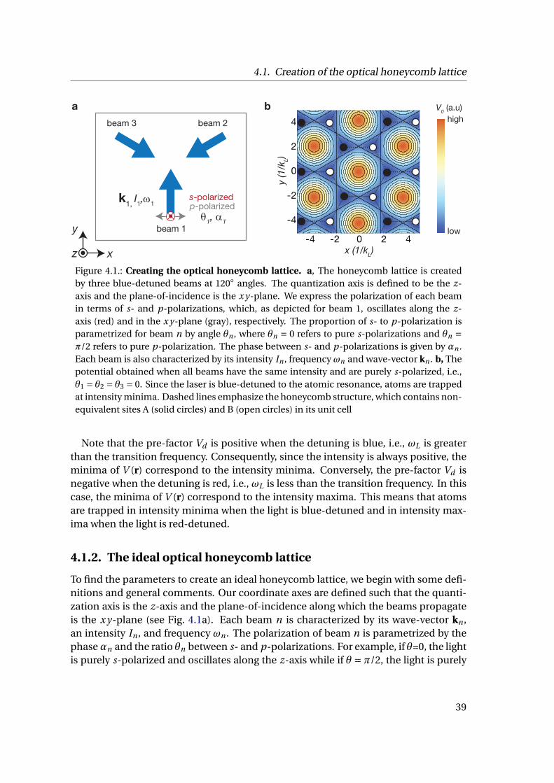
4.1. Creation of the optical honeycomb lattice
a b
x
y
z-4 -2 0 2 4
-4
-2
0
2
4
x (1/kL)
y (1
/kL)
V0 (a.u)high
low
k1, I1,ω1 p-polarizeds-polarized
θ1, α1beam 1
beam 2beam 3
Figure 4.1.: Creating the optical honeycomb lattice. a, The honeycomb lattice is createdby three blue-detuned beams at 120 angles. The quantization axis is defined to be the z-axis and the plane-of-incidence is the x y-plane. We express the polarization of each beamin terms of s- and p-polarizations, which, as depicted for beam 1, oscillates along the z-axis (red) and in the x y-plane (gray), respectively. The proportion of s- to p-polarization isparametrized for beam n by angle θn , where θn = 0 refers to pure s-polarizations and θn =π/2 refers to pure p-polarization. The phase between s- and p-polarizations is given by αn .Each beam is also characterized by its intensity In , frequency ωn and wave-vector kn . b, Thepotential obtained when all beams have the same intensity and are purely s-polarized, i.e.,θ1 = θ2 = θ3 = 0. Since the laser is blue-detuned to the atomic resonance, atoms are trappedat intensity minima. Dashed lines emphasize the honeycomb structure, which contains non-equivalent sites A (solid circles) and B (open circles) in its unit cell
Note that the pre-factor Vd is positive when the detuning is blue, i.e., ωL is greaterthan the transition frequency. Consequently, since the intensity is always positive, theminima of V (r) correspond to the intensity minima. Conversely, the pre-factor Vd isnegative when the detuning is red, i.e., ωL is less than the transition frequency. In thiscase, the minima of V (r) correspond to the intensity maxima. This means that atomsare trapped in intensity minima when the light is blue-detuned and in intensity max-ima when the light is red-detuned.
4.1.2. The ideal optical honeycomb lattice
To find the parameters to create an ideal honeycomb lattice, we begin with some defi-nitions and general comments. Our coordinate axes are defined such that the quanti-zation axis is the z-axis and the plane-of-incidence along which the beams propagateis the x y-plane (see Fig. 4.1a). Each beam n is characterized by its wave-vector kn ,an intensity In , and frequency ωn . The polarization of beam n is parametrized by thephaseαn and the ratio θn between s- and p-polarizations. For example, if θ=0, the lightis purely s-polarized and oscillates along the z-axis while if θ = π/2, the light is purely
39
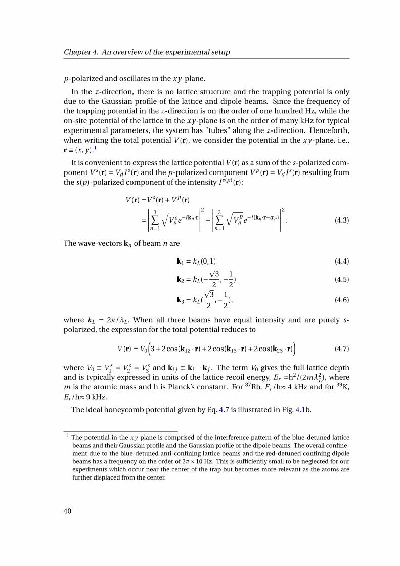
Chapter 4. An overview of the experimental setup
p-polarized and oscillates in the x y-plane.
In the z-direction, there is no lattice structure and the trapping potential is onlydue to the Gaussian profile of the lattice and dipole beams. Since the frequency ofthe trapping potential in the z-direction is on the order of one hundred Hz, while theon-site potential of the lattice in the x y-plane is on the order of many kHz for typicalexperimental parameters, the system has "tubes" along the z-direction. Henceforth,when writing the total potential V (r), we consider the potential in the x y-plane, i.e.,r ≡ (x, y).1
It is convenient to express the lattice potential V (r) as a sum of the s-polarized com-ponent V s(r) =Vd I s(r) and the p-polarized component V p (r) =Vd I s(r) resulting fromthe s(p)-polarized component of the intensity I s(p)(r):
V (r) =V s(r)+V p (r)
=∣∣∣∣∣ 3∑n=1
√V s
n e−i kn ·r∣∣∣∣∣2
+∣∣∣∣∣ 3∑n=1
√V p
n e−i (kn ·r−αn )
∣∣∣∣∣2
. (4.3)
The wave-vectors kn of beam n are
k1 = kL(0,1) (4.4)
k2 = kL(−p
3
2,−1
2) (4.5)
k3 = kL(
p3
2,−1
2), (4.6)
where kL = 2π/λL . When all three beams have equal intensity and are purely s-polarized, the expression for the total potential reduces to
V (r) =V0
(3+2cos(k12 · r)+2cos(k13 · r)+2cos(k23 · r)
)(4.7)
where V0 ≡ V s1 = V s
2 = V s3 and ki j ≡ ki −k j . The term V0 gives the full lattice depth
and is typically expressed in units of the lattice recoil energy, Er =h2/(2mλ2L), where
m is the atomic mass and h is Planck’s constant. For 87Rb, Er /h≈ 4 kHz and for 39K,Er /h≈ 9 kHz.
The ideal honeycomb potential given by Eq. 4.7 is illustrated in Fig. 4.1b.
1 The potential in the x y-plane is comprised of the interference pattern of the blue-detuned latticebeams and their Gaussian profile and the Gaussian profile of the dipole beams. The overall confine-ment due to the blue-detuned anti-confining lattice beams and the red-detuned confining dipolebeams has a frequency on the order of 2π×10 Hz. This is sufficiently small to be neglected for ourexperiments which occur near the center of the trap but becomes more relevant as the atoms arefurther displaced from the center.
40
4.1. Creation of the optical honeycomb lattice
V0 (a.u)high
lowy
x
δ1
δ2
δ3
1
23
Figure 4.2.: Realizing non-isotropic tunneling. When all beams have equal intensities, thehopping amplitudes along directions δ1,δ2, and δ3 are equivalent (center). Non-isotropictunneling occurs when the intensity of, e.g., beam 1 is changed. When the intensity of beam1 is decreased (light blue arrow, left panel), the tunneling amplitude along δ3 decreases com-pared to the tunneling amplitude along δ1 and δ2. When the intensity of beam is increased(dark blue arrow, right panel), the tunneling amplitude along δ3 increases.
4.1.3. Modifications on the ideal: non-isotropic tunneling andadding a Semenoff mass
Control over both the intensity and polarization of each beam affords the optical hon-eycomb lattice a high degree of tunability. For example, by changing the intensity ofa single beam, both the real-space and reciprocal-space structure of the honeycomblattice can be modified [31, 78, 102]. By changing the polarization of the beams, thehoneycomb lattice can become state-dependent [28, 103] or tuned into a triangularlattice [28]. In this section, we focus on experimentally implementing two methods ofC3-symmetry breaking: non-isotropic tunneling and the Semenoff mass.
Realizing non-isotropic tunneling
In the ideal honeycomb lattice, the magnitude of the hopping is equivalent in all threedirections, δ1,δ2, and δ3. The simplest way to break this equivalence is to change theintensity of the beams. For a purely s-polarized potential where the beams have in-equivalent intensities and contribute a potential V1,V2, and V3, where V j refers to thepotential due to beam j , the total potential is
V (r) =V1 +V2 +V3 +2√
V1V2 cos(k12 · r)
+2√
V1V3 cos(k13 · r)+2√
V2V3 cos(k23 · r) (4.8)
By changing the intensity of a single beam, we obtain a different potential barrieralong one hopping direction and have therefore broken C3 symmetry. The effect ofthis real-space change in reciprocal space is to shift the positions of the Dirac points,as was discussed in Sec. 3.2.3.
41
Chapter 4. An overview of the experimental setup
Realizing a Semenoff mass
To realize a Semenoff mass, we constrain the polarizations of each beam to have thesame (non-zero) composition of s- and p-polarizations, i.e., θ1 = θ2 = θ2 ≡ θ. The po-tentials arising from the interference of the s- and p- components of the three beams,which are shown separately in Fig. 4.3, have the form
V s(r) =V0 cos2θ(3+2cos(k12 · r)+2cos(k13 · r)+2cos(k23 · r)
)(4.9)
and
V p (r) =V0 sin2θ
(3−cos(k12 · r+α12)−cos(k13 · r+α13)−cos(k23 · r+α23)
)(4.10)
where αi j ≡ αi −α j . Note that in defining the same V0 for the s- and p-polarizations,we have neglected the state-dependence of the dipole potential, which is valid in ourcase of far-detuned light2.
By choosing the phase αn of each beam, we can shift the p-polarized potential rela-
2As a rough justification of this approximation, we note that Eq. 4.1 can be written as
V (r) = (2VD2 +VD1 +∆V P mF gF )I (r),
where we have defined
VD1(D2) =πc2ΓD1(D2)
2ω3D1(D2)
1
∆D1(D2)
∆V =VD2 −VD1.
The intensity can be separated into its polarization components as I (r) = I s (r)+ I p (r). Furthermore,we note that in our coordinate system, I s (r) = Iπ(r) and I p (r) = Iσ
+(r)+ Iσ
−(r). By substituting the
polarization-separated intensity into the expression for I (r), we clearly see that the potential is com-prised of a state-independent and a state-dependent part:
V (r) = (2VD2 +VD1 +∆V P mF gF )(Iπ(r)+ Iσ+
(r)+ Iσ−
(r))
= (2VD2 +VD1)I (r)+∆V mF gF (Iσ+
(r)− Iσ−
(r)),
where we have used that P = 0,±1 for π and σ± light in the second line. In neglecting the stateindependent part, our assumption is that
∆V mF gF (Iσ+
(r)− Iσ−
(r))
(2VD2 +VD1)I (r)¿ 1 (4.11)
Due to our large detuningω−ωL , the term∆V mF gF /(2VD2+VD1) is on the order 15%. Furthermore,the term (Iσ
+(r)− Iσ
−(r))/I (r) is maximally 1, but is, for experimentally relevant values of θ, on the
order of 10%. The product of these two terms yields that the state-dependent part of the potentialcontributes only on the percent level to the total potential. Hence, our approximation to neglect thestate-dependent part is valid. Ref. [78] contains a detailed derivation of the potential in terms of itspolarization components.
42

4.1. Creation of the optical honeycomb lattice
-4 -2 0 2 4
-4
-2
0
2
4
-4 -2 0 2 4 -4 -2 0 2 4
a
b
x (1/kL )
-4
-2
0
2
4
y (1
/kL )
V0 (a.u)high
lowy (1
/kL )
x (1/kL ) x (1/kL )
V s
(r) V (r)V p
(r)
Figure 4.3.: Realizing the Semenoff mass. We add an energy offset between A and B sublat-tice sites while maintaining isotropic tunneling by tuning the proportion of and phase be-tween the s- and p-polarizations of each beam. The p-polarized (left), s-polarized (center),and total potential (right) are shown for θ = π/4. The lattice structure is outlined in dashedgray lines with black (white) dots representing A (B) sites in the total potential. In a, bothpolarization components are in-phase, i.e., α1 = α2 = α3 = 0. Note that for the p-polarizedpotential, the minima form a triangular lattice. In b, α1 = 0,α2 = 2π/3, and α3 = 4π/3. Withthese parameters, the potential minima of the s-polarized potential coincide with the min-ima of the p-polarized potential on A sites and the maxima of the p-polarized potential on Bsites. Hence, there is an energy difference between A and B sites in the total potential.
43
Chapter 4. An overview of the experimental setup
tive to the s-polarized potential. Whenα1 =α2 =α3 = 0, the minima of the p-polarizedpotential and the maximima of the s-polarized potential coincide with the A and B sites(Fig. 4.3a). Consequently, atoms experience the same ac Stark shift on either an A orB site. However, by setting α12 = α23 = 4π/3 and α13 = 2π/3, the s-polarized potentialis shifted such that the potential maxima occur on B sites while the potential minimaoccur on A sites (Fig. 4.3b). Consequently, the potential on A sites is lower than thepotential on B sites, as illustrated in the right-most column of Fig. 4.3b.
4.2. State preparation: creating a BEC
The starting point of all experiments described in this thesis is the adiabatic loadingof a BEC of either 87Rb or 39K into an optical honeycomb lattice. To obtain a BEC, wecool an atomic vapor of 87Rb and/or 39K. When a 87Rb BEC is desired, only 87Rb iscooled. When a 39K BEC is desired, we cool both 39K and 87Rb atoms for later use insympathetic cooling. The cooling process begins in a two-species 2D+MOT [104–110],as shown in Fig. 4.4. From the 2D+MOT, the atoms enter the 3D-MOT [111], wherefurther cooling occurs. At the end of the 3D-MOT, the magnetic fields are switched offand the atoms are again cooled by an optical molasses [111]. Next, both 39K and 87Rbatoms are spin-polarized into their |F = 2,mF = 2⟩ state in preparation for magnetictransport. The atoms are then transported by a 100 G/cm magnetic quadrupole trapformed by pairs of overlapping coils [112]. We ramp the current through each pairof coils such that a magnetic quadrupole potential smoothly moves the atoms a totaldistance of 58cm from the 3D-MOT to the science cell.
Once the atoms reach the science cell, we begin microwave evaporation in aplugged quadrupole trap. The center of the quadrupole trap is plugged with a tightly-focused, blue-detuned beam in order to avoid Majorana losses [113–115]. Next, as thequadrupole gradient is being ramped down to zero, the intensity of a pair of crosseddipole beams is ramped up to initiate further evaporative cooling in the crossed-dipoletrap until condensation. Soon after the crossed-dipole trap has been ramped up, weperform an RF-sweep to transfer both 87Rb and 39K into their F=1 ground state man-ifold and blow away residual F=2 atoms via a resonant light-pulse. Evaporative cool-ing then proceeds with only F=1 atoms, thereby avoiding possible spin-changing colli-sions.
When cooling only 87Rb, we simply lower the intensity of the dipole beams. Thecrossed-beam dipole trap is formed from light of wavelength 1064 nm and is thereforered-detuned from the atomic transition. Hence, based on Eq. 4.1, a lower intensitymeans a lower trapping potential, from which hot atoms can escape. The remainingatoms efficiently thermalize to a lower temperature and eventually condense.
Condensation of 39K is achieved using the same principle, but we must addition-ally utilize Feshbach resonances, which allow us to tune the scattering length betweenatoms via a magnetic offset field [38] for efficient thermalization. We first utilize a Fes-
44

4.3. State evolution: creating a gradient
Ion pump
2D+ MOT
Glass science cell
3D MOT
Ion pump
a b
x
y
z
Transport coils in cooling block
Figure 4.4.: Experimental setup for preparing a BEC. a, An overview of the vacuum setupwith the path of the atoms shown in red. Atoms begin in the 2D+MOT, where they are pre-cooled before traveling into the 3D-MOT chamber for further cooling. Next, the atoms aremagnetically transported to the science cell, where they are evaporatively cooled to quantumdegeneracy before the experiments occur. b, The glass science cell has an asymmetric shape(black outline) to avoid back-reflections of beams onto the atoms (black dot) from the innersurface of the glass. The lattice beams (blue) propagate at 120 degree angles onto the atoms.The dipole beams (red) propagate perpendicular to each other, forming the crossed-dipoletrap. One dipole beam propagates nearly on the same axis as one of the lattice beams. Themain imaging beam (orange circle with cross)is centered on the atoms and travels verticallyinto the plane.
hbach resonance between 39K and 87Rb atoms, sympathetically cooling the 39K atomswith the microwave-evaporated 87Rb atoms [116, 117]. During this time, we continu-ously lower the dipole trap depth. Once the 87Rb atoms have dropped out of the trapdue to their larger mass, we use another Feshbach resonance between 39K atoms andcontinue evaporation until condensation [118]. We then decrease the scattering lengthto avoid losses before ramping the field to the desired scattering length for the experi-ments. Further details can be found in Appendix A.
After condensation has occured, the atoms are held in the low-intensity dipole trapas the intensity of the lattice beams is adiabatically ramped up. When the lattice is sta-tionary with respect to the atomic cloud, the BEC macroscopically occupies the groundstate of the lattice, given by the Bloch state |Ψ1
Γ⟩ at quasimomentum Γ in the first band.
4.3. State evolution: creating a gradient
In the presence of a constant external force, the quasimomentum of a Bloch state be-comes time-dependent [89]. In this section, we review how this force is realized us-ing either a magnetic field or by accelerating the lattice. While the force due to themagnetic field gradient is spin-dependent, the force due to the lattice acceleration isspin-independent. As we will later explain in Chapter 5, both a spin-dependent and a
45
Chapter 4. An overview of the experimental setup
spin-independent force is required to measure the Berry phase. Measuring elementsof the Wilson line requires only a spin-independent force.
4.3.1. Magnetic field
To create a magnetic field gradient, we use a single coil oriented along the x-axis, asshown in Fig. 4.5a. The positioning and geometry of the coil was chosen to maximizethe force felt by the atoms. The coil is conically shaped in order to fit as close as possi-ble to the experimental cell without obstructing the dipole and lattice beams. Since themagnetic field is proportional to the current, we could try to compensate for the dis-tance between the coil and the atoms by sending more current. However, this wouldresult in excess heating of the coil.
Near the position of the atoms, the magnitude of the magnetic field created by thecoil is, to first order, Ba(r) = B0 +∇B · r, where ∇B is the magnetic field gradient cre-ated by the coil evaluated at the position of the atoms. Due to the Zeeman effect, themagnetic field breaks the energy degeneracy between the magnetic sublevels mF ofthe hyperfine level F as
E(r) =µB mF gF Ba(r), (4.12)
where µB is the Bohr magneton and gF is the Landé g-factor. Since the coil is orientedalong the x-axis, the linear gradient E(r) is predominantly in the x-direction. Further-more, this gradient is associated with a force
F =∇E(r) =µB mF gF∇B (4.13)
Due to the dependence on gF and mF , the force will be different for different hyperfinestates.
4.3.2. Lattice acceleration
How do we accelerate the lattice?
To understand the acceleration of the lattice, it is instructive to first consider the inter-ference pattern formed by two counterpropagating beams along the x-direction. If thefrequencies of the beams are the same, the resulting interference pattern is a stand-ing wave. If, however, there is a frequency difference between the counterpropogatingbeams, the total interference pattern now moves with a velocity proportional to thefrequency difference. Accordingly, if the frequency difference is time-dependent, thenthe total interference pattern moves with a time-dependent velocity. In this case, wesay that the lattice is accelerating.
The same reasoning applies to the honeycomb lattice. Changing the frequency of,for example, beam 1 propagating along the y-direction, moves the entire interference
46

4.3. State evolution: creating a gradient
pattern along the y-direction, as illustrated in Fig. 4.5b. The velocity with which thelattice potential moves is
vy (t ) = 2
3λδν, (4.14)
where δν is the frequency difference between beam 1 and the other two beams. Itfollows that the acceleration of the lattice in the y-direction is given by
ay (t ) = d v(t )/d t = 2
3λ
d
d tδν. (4.15)
Generally, sweeping the frequency of beam i results in acceleration along the propaga-tion direction of beam i . The acceleration due to a frequency sweep of two beams is thevector sum of the accelerations from each individual beam. By tuning the parameterd
d t δν, which parametrizes the rate of the frequency sweep, we can tune the magnitudeof the acceleration of the lattice. Hence, by independently controlling the frequenciesof two beams, we can accelerate the lattice along arbitrary paths. In our experiments,we choose the frequency sweep rate d
d t δν to be constant to obtain a constant acceler-ation.
a b
+
=
-4 -2 0 2 4
-4
-2
0
2
4
x (1/kL)
y (1
/kL)
-4 -2 0 2 4x (1/kL)
V0 (a.u)high
low
x
y
ωω
ω
ω
ω+δω
ω
x
V(x)
Figure 4.5.: Methods of creating a force for state-evolution: magnetic field gradient and lat-tice acceleration. a, A (not-to-scale) schematic showing the relative positions of the latticebeams (blue arrows), atoms (red dot), and coil (brown conical shape). The single coil is cen-tered along the position of the atoms and creates a magnetic field gradient along the x-axis.The resulting potential along the x-direction (bottom blue in the inset box) is the sum of theoriginal lattice potential (top blue) and the gradient potential (brown). b, By changing thefrequency of beam n by δω while keeping the frequency of the other two beams fixed, theentire potential shifts along the propagation direction of beam n. We show the position ofthe potential at two different times for a constant frequency shift in beam 1, which movesthe lattice potential along the y-axis.
47
Chapter 4. An overview of the experimental setup
How does lattice acceleration create a gradient?
The lattice acceleration is equivalent to a gradient in the frame co-moving with the lat-tice. This can be seen by by first writing the time-dependent Hamiltonian for a latticepotential with varying position R(t ):
H(t ) = p2
2m+V (r−R (t )), (4.16)
where p and r are the momentum and position operators, respectively. To enter a frameco-moving with the lattice we use the a unitary transformation
U (t ) = e−i mR(t )·re i R(t )·p, (4.17)
where ħ= 1 and m is the atomic mass. These are translation operators of real and mo-mentum space. Hence, the unitary transformation takes into account both the vary-ing position and momentum of the atoms. The time-dependent Schrödinger equationiΨ= H(t )Ψ can then equivalently be expressed as i ˙Ψ= HΨ, where Ψ=UΨ and
H =U HU † + iUU † (4.18)
Noting that
U HU † = (p2 +m ˙R(t ))2
2m+V (r),
iUU † = mR(t ) · r− R(t ) · (p+mR(t )), (4.19)
we arrive at
H = p2
2m+V (r)+mR(t ) · r− mR(t )2
2(4.20)
In the co-moving frame, the atoms experience a force F =−mR(t ), i.e., in the opposite
direction of the lattice movement. The term mR(t )2
2 is an energy offset associated withthe momentum mR(t ) imparted by the moving lattice.
4.4. State detection: absorption imaging
Information about our atoms are attained through absorption imaging, one of themost standard techniques in ultracold atom experiments [119]. In absorption imaging,we shine a collimated beam of resonant light onto the atoms. The density-dependentintensity profile I (x, y) is then imaged onto a charge-coupled-device (CCD) camera.According to the Beer-Lambert law, an imaging beam propagating in the z-direction
48
4.4. State detection: absorption imaging
through an atomic sample with density n(x, y, z) has resultant intensity[120]
I (x, y) = I0eσ∫
n(x,y,z)d z
= I0eσncol (x,y), (4.21)
where ncol (x, y) is called the local column density and σ is the scattering cross-sectionof the atoms, which takes into account details of the atomic level structure and theintensity and polarization of the imaging beam. Solving for the local column density,which is the quantity of interest, we obtain
ncol (x, y) =− 1
σln
I (x, y)
I0(x, y)(4.22)
Experimentally, we obtain ncol (x, y) by taking four images: 1) one image with theatoms and the imaging beam, 2) one image with only the imaging beam, and 3) and 4)two dark images with neither atoms nor imaging beam to account for stray light hittingthe CCD chip. Image 3 is then subtracted from image 1, to give I (x, y), and image 4 issubtracted from image 2, to give I0(x, y).
In these experiments, we image the atoms after they have been released from allconfining potentials and have undergone free-flight expansion for a given time. Thesetime-of-flight (TOF) images reveal different aspects of the momentum composition ofthe atoms, depending on whether we suddenly shut off or gradually ramp down thelattice potential. The former method is primarily used to ensure that all three beamshave equal intensity at the position of the atoms, such that the lattice is as ideal aspossible. The latter method is used for state-detection in the experiments.
4.4.1. Sudden shut-off of the lattice: plane-wave decomposition
Assume we have adiabatically loaded the BEC into the lattice at q = Γ in the first band.When the lattice is suddenly shut off, the Bloch state |Ψ1
Γ⟩ is projected onto the realspace momentum states. In other words, a sudden shut-off of the lattice probes the(modulus-squared) coefficients of the plane wave expansion of the Bloch state. Recallfrom Eq. 3.33 that the plane wave expansion of un
q (r) is comprised only of reciprocallattice vectors. Consequently, as shown in Fig. 4.6a, only momenta that are a linearcombination of the primitive reciprocal lattice vectors b1 and b2 are occupied. In otherwords, a sudden shut-off of the real-space lattice images the reciprocal lattice points.These plane wave components are commonly called Bragg peaks or coherence peaks.
However, the Bloch state is of course not an equal superposition of all plane waves.This can be understood intuitively by noting that the BEC occupies a single plane wavestate without a lattice. As the lattice depth is increased, the potential deviates morefrom the free-space potential. Consequently, we require more plane waves to con-
49
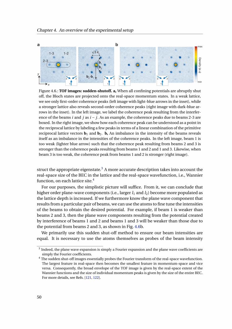
Chapter 4. An overview of the experimental setup
a b
Density (a.u)
min
max
x
y
2-3
1-21-3
b1b2
b2-b1
3 kL
1
23
1
23
1
23
1
23
Figure 4.6.: TOF images: sudden-shutoff. a, When all confining potentials are abruptly shutoff, the Bloch states are projected onto the real-space momentum states. In a weak lattice,we see only first-order coherence peaks (left image with light-blue arrows in the inset), whilea stronger lattice also reveals second-order coherence peaks (right image with dark-blue ar-rows in the inset). In the left image, we label the coherence peak resulting from the interfer-ence of the beams i and j as i − j . As an example, the coherence peaks due to beams 2-3 areboxed. In the right image, we show how each coherence peak can be understood as a point inthe reciprocal lattice by labeling a few peaks in terms of a linear combination of the primitivereciprocal lattice vectors b1 and b2. b, An imbalance in the intensity of the beams revealsitself as an imbalance in the intensities of the coherence peaks. In the left image, beam 1 istoo weak (lighter blue arrow) such that the coherence peak resulting from beams 2 and 3 isstronger than the coherence peaks resulting from beams 1 and 2 and 1 and 3. Likewise, whenbeam 3 is too weak, the coherence peak from beams 1 and 2 is stronger (right image).
struct the appropriate eigenstate.3 A more accurate description takes into account thereal-space size of the BEC in the lattice and the real-space wavefunction, i.e., Wannierfunction, on each lattice site.4
For our purposes, the simplistic picture will suffice. From it, we can conclude thathigher order plane-wave components (i.e., larger l1 and l2) become more populated asthe lattice depth is increased. If we furthermore know the plane wave component thatresults from a particular pair of beams, we can use the atoms to fine tune the intensitiesof the beams to obtain the desired potential. For example, if beam 1 is weaker thanbeams 2 and 3, then the plane wave components resulting from the potential createdby interference of beams 1 and 2 and beams 1 and 3 will be weaker than those due tothe potential from beams 2 and 3, as shown in Fig. 4.6b.
We primarily use this sudden shut-off method to ensure our beam intensities areequal. It is necessary to use the atoms themselves as probes of the beam intensity
3 Indeed, the plane wave expansion is simply a Fourier expansion and the plane wave coefficients aresimply the Fourier coefficients.
4 The sudden shut-off images essentially probes the Fourier transform of the real-space wavefunction.The largest feature in real-space then becomes the smallest feature in momentum-space and viceversa. Consequently, the broad envelope of the TOF image is given by the real-space extent of theWannier functions and the size of individual momentum peaks is given by the size of the entire BEC.For more details, see Refs. [121, 122].
50
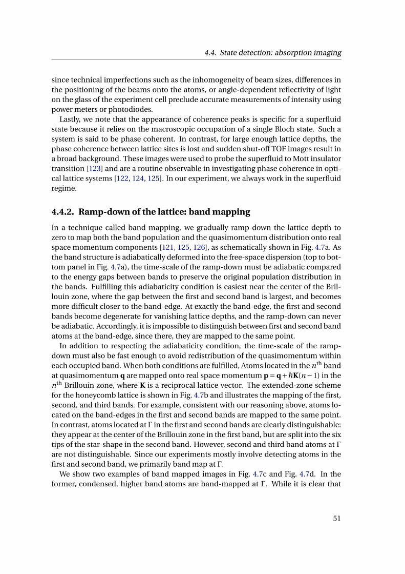
4.4. State detection: absorption imaging
since technical imperfections such as the inhomogeneity of beam sizes, differences inthe positioning of the beams onto the atoms, or angle-dependent reflectivity of lighton the glass of the experiment cell preclude accurate measurements of intensity usingpower meters or photodiodes.
Lastly, we note that the appearance of coherence peaks is specific for a superfluidstate because it relies on the macroscopic occupation of a single Bloch state. Such asystem is said to be phase coherent. In contrast, for large enough lattice depths, thephase coherence between lattice sites is lost and sudden shut-off TOF images result ina broad background. These images were used to probe the superfluid to Mott insulatortransition [123] and are a routine observable in investigating phase coherence in opti-cal lattice systems [122, 124, 125]. In our experiment, we always work in the superfluidregime.
4.4.2. Ramp-down of the lattice: band mapping
In a technique called band mapping, we gradually ramp down the lattice depth tozero to map both the band population and the quasimomentum distribution onto realspace momentum components [121, 125, 126], as schematically shown in Fig. 4.7a. Asthe band structure is adiabatically deformed into the free-space dispersion (top to bot-tom panel in Fig. 4.7a), the time-scale of the ramp-down must be adiabatic comparedto the energy gaps between bands to preserve the original population distribution inthe bands. Fulfilling this adiabaticity condition is easiest near the center of the Bril-louin zone, where the gap between the first and second band is largest, and becomesmore difficult closer to the band-edge. At exactly the band-edge, the first and secondbands become degenerate for vanishing lattice depths, and the ramp-down can neverbe adiabatic. Accordingly, it is impossible to distinguish between first and second bandatoms at the band-edge, since there, they are mapped to the same point.
In addition to respecting the adiabaticity condition, the time-scale of the ramp-down must also be fast enough to avoid redistribution of the quasimomentum withineach occupied band. When both conditions are fulfilled, Atoms located in the nth bandat quasimomentum q are mapped onto real space momentum p = q+ħK(n −1) in thenth Brillouin zone, where K is a reciprocal lattice vector. The extended-zone schemefor the honeycomb lattice is shown in Fig. 4.7b and illustrates the mapping of the first,second, and third bands. For example, consistent with our reasoning above, atoms lo-cated on the band-edges in the first and second bands are mapped to the same point.In contrast, atoms located at Γ in the first and second bands are clearly distinguishable:they appear at the center of the Brillouin zone in the first band, but are split into the sixtips of the star-shape in the second band. However, second and third band atoms at Γare not distinguishable. Since our experiments mostly involve detecting atoms in thefirst and second band, we primarily band map at Γ.
We show two examples of band mapped images in Fig. 4.7c and Fig. 4.7d. In theformer, condensed, higher band atoms are band-mapped at Γ. While it is clear that
51
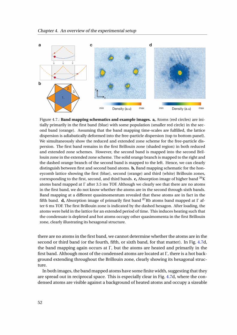
Chapter 4. An overview of the experimental setup
a
b
c
1.
2.3.
Density (a.u)min max Density (a.u)min max
y
x
d
Figure 4.7.: Band mapping schematics and example images. a, Atoms (red circles) are ini-tially primarily in the first band (blue) with some population (smaller red circle) in the sec-ond band (orange). Assuming that the band mapping time-scales are fulfilled, the latticedispersion is adiabatically deformed into the free-particle dispersion (top to bottom panel).We simultaneously show the reduced and extended zone scheme for the free-particle dis-persion. The first band remains in the first Brillouin zone (shaded region) in both reducedand extended zone schemes. However, the second band is mapped into the second Bril-louin zone in the extended zone scheme. The solid orange branch is mapped to the right andthe dashed orange branch of the second band is mapped to the left. Hence, we can clearlydistinguish between first and second band atoms. b, Band mapping schematic for the hon-eycomb lattice showing the first (blue), second (orange) and third (white) Brillouin zones,corresponding to the first, second, and third bands. c, Absorption image of higher band 39Katoms band mapped at Γ after 3.5 ms TOF. Although we clearly see that there are no atomsin the first band, we do not know whether the atoms are in the second through sixth bands.Band mapping at a different quasimomentum revealed that these atoms are in fact in thefifth band. d, Absorption image of primarily first band 87Rb atoms band mapped at Γ af-ter 6 ms TOF. The first Brillouin zone is indicated by the dashed hexagon. After loading, theatoms were held in the lattice for an extended period of time. This induces heating such thatthe condensate is depleted and hot atoms occupy other quasimomenta in the first Brillouinzone, clearly illustrating its hexagonal structure.
there are no atoms in the first band, we cannot determine whether the atoms are in thesecond or third band (or the fourth, fifth, or sixth band, for that matter). In Fig. 4.7d,the band mapping again occurs at Γ, but the atoms are heated and primarily in thefirst band. Although most of the condensed atoms are located at Γ, there is a hot back-ground extending throughout the Brillouin zone, clearly showing its hexagonal struc-ture.
In both images, the band mapped atoms have some finite width, suggesting that theyare spread out in reciprocal space. This is especially clear in Fig. 4.7d, where the con-densed atoms are visible against a background of heated atoms and occupy a sizeable
52
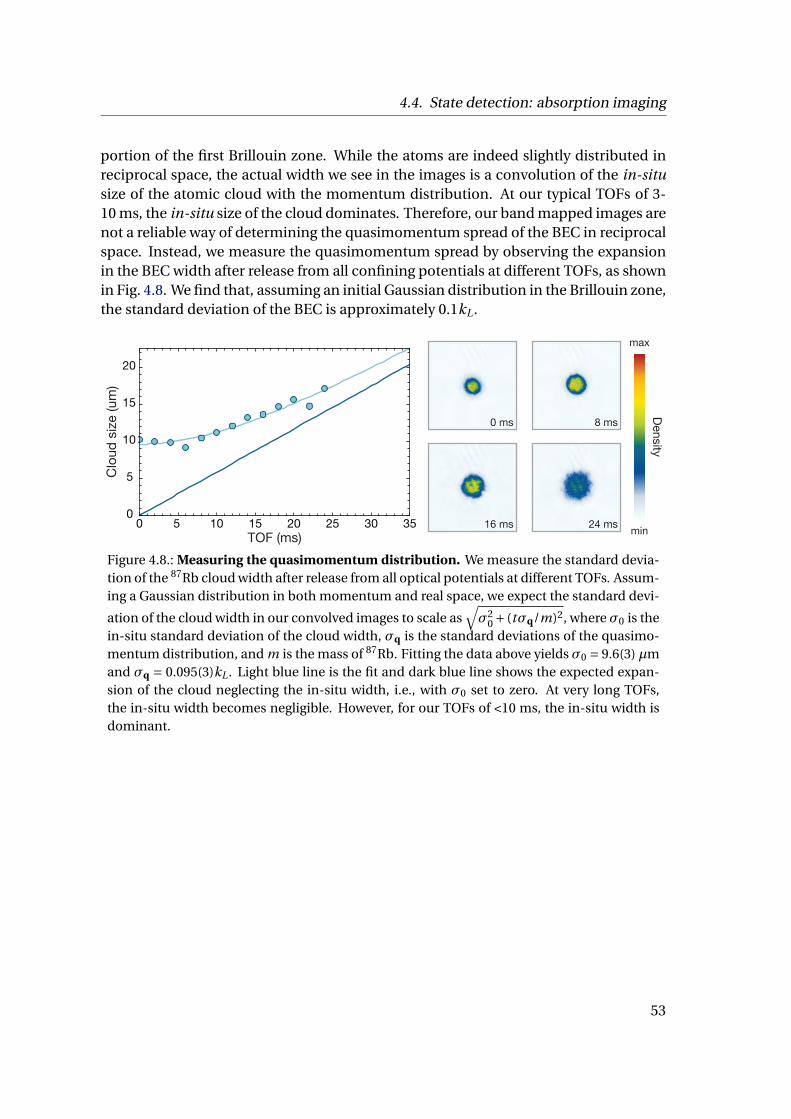
4.4. State detection: absorption imaging
portion of the first Brillouin zone. While the atoms are indeed slightly distributed inreciprocal space, the actual width we see in the images is a convolution of the in-situsize of the atomic cloud with the momentum distribution. At our typical TOFs of 3-10 ms, the in-situ size of the cloud dominates. Therefore, our band mapped images arenot a reliable way of determining the quasimomentum spread of the BEC in reciprocalspace. Instead, we measure the quasimomentum spread by observing the expansionin the BEC width after release from all confining potentials at different TOFs, as shownin Fig. 4.8. We find that, assuming an initial Gaussian distribution in the Brillouin zone,the standard deviation of the BEC is approximately 0.1kL .
0 5 10 15 20 25 30 350
5
10
15
20
TOF (ms)
Clo
ud s
ize (u
m)
Density
min
max
0 ms 8 ms
16 ms 24 ms
Figure 4.8.: Measuring the quasimomentum distribution. We measure the standard devia-tion of the 87Rb cloud width after release from all optical potentials at different TOFs. Assum-ing a Gaussian distribution in both momentum and real space, we expect the standard devi-
ation of the cloud width in our convolved images to scale as√σ2
0 + (tσq/m)2, whereσ0 is thein-situ standard deviation of the cloud width, σq is the standard deviations of the quasimo-mentum distribution, and m is the mass of 87Rb. Fitting the data above yields σ0 = 9.6(3) µmand σq = 0.095(3)kL . Light blue line is the fit and dark blue line shows the expected expan-sion of the cloud neglecting the in-situ width, i.e., with σ0 set to zero. At very long TOFs,the in-situ width becomes negligible. However, for our TOFs of <10 ms, the in-situ width isdominant.
53

Chapter 4. An overview of the experimental setup
4.5. Applications: Bloch oscillations and lattice depthcalibration
We conclude this chapter by applying the tools described in previous sections to exam-ine Bloch oscillations and calibrate the lattice depth. We show the difference in Blochoscillations between applying a small force, such that the evolution is adiabatic, and alarge force, such that the second band is also populated. Next, we utilize our ability tomove along arbitrary paths in the Brillouin zone with a non-adiabatic force to calibratethe lattice depth through a technique called Stueckelberg interferometry.
4.5.1. Bloch oscillations
Bloch oscillations originate from solid state physics and describe the response of anelectron in a perfect crystal to a constant electric field [1]. In contrast to a free-particlewhich accelerates uniformly along the field, Bloch electrons oscillate in real space.When we refer to Bloch oscillations here, we refer to the motion of the atoms in re-ciprocal space, where the quasimomentum scans the Brillouin zone at a rate linearlyproportional to the applied force. When the atoms have moved by one reciprocal lat-tice vector, we say that it has undergone a single Bloch oscillation. Although the move-ment in reciprocal space is related to the movement in real space, we cannot resolvethe real space movement in our experiment and restrict ourselves to looking at Blochoscillations in reciprocal space. The connection between real space Bloch oscillationsand reciprocal space movement in the context of cold atoms is detailed in Refs. [89,127, 128].
In Fig. 4.9, we show bandmapped images of atoms undergoing adiabatic Bloch oscil-lations due to a magnetic gradient and accelerating the lattice along the Γ-M direction.In the case of the gradient (Fig. 4.9a), the atoms move as they scan the Brillouin zone,which remains fixed in the lab frame. Here, the real space momentum we see directlygives the quasimomentum. In contrast, in the case of lattice acceleration (Fig. 4.9b),the atoms seem stationary. This is because their real space momentum consists ofboth the quasimomentum and the momentum imparted by the lattice, which is givenby the last term of Eq. 4.20. Furthermore, recall that the force the atoms experience is inthe opposite direction as the movement of the lattice. Hence, for a lattice moving withspeed |v | = |F| t/m at time t , where F is the applied force and m is the atomic mass, thereal space momentum is given by the difference between the quasimomentum, |F| tand the lattice momentum m |v | = |F| t . This difference is zero until the atoms reachthe edge of the Brillouin zone and suddenly Bragg-reflect to the opposite edge of theBrillouin zone. In the bottom row of Fig. 4.9b, we show band mapped images of atomsundergoing non-adiabatic Bloch oscillations due to lattice acceleration. The popula-tion in the second band is clearly visible after the atoms traverse the Brillouin zoneedge.
54
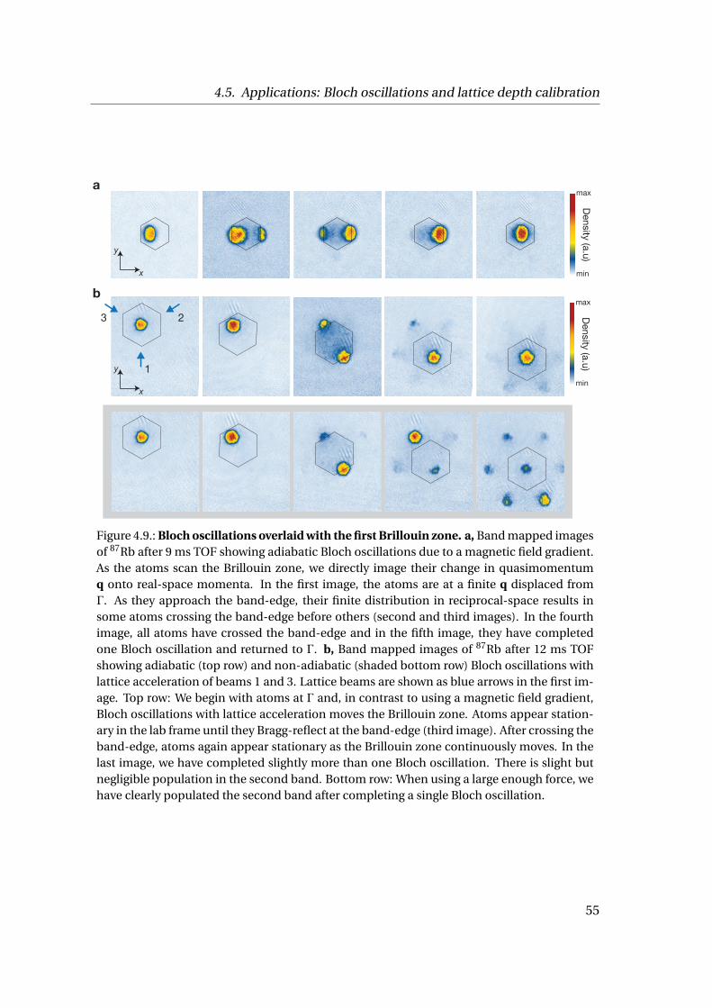
4.5. Applications: Bloch oscillations and lattice depth calibration
a
b
Density (a.u)
max
min
Density (a.u)
max
min
y
x
y
x
1
23
Figure 4.9.: Bloch oscillations overlaid with the first Brillouin zone. a, Band mapped imagesof 87Rb after 9 ms TOF showing adiabatic Bloch oscillations due to a magnetic field gradient.As the atoms scan the Brillouin zone, we directly image their change in quasimomentumq onto real-space momenta. In the first image, the atoms are at a finite q displaced fromΓ. As they approach the band-edge, their finite distribution in reciprocal-space results insome atoms crossing the band-edge before others (second and third images). In the fourthimage, all atoms have crossed the band-edge and in the fifth image, they have completedone Bloch oscillation and returned to Γ. b, Band mapped images of 87Rb after 12 ms TOFshowing adiabatic (top row) and non-adiabatic (shaded bottom row) Bloch oscillations withlattice acceleration of beams 1 and 3. Lattice beams are shown as blue arrows in the first im-age. Top row: We begin with atoms at Γ and, in contrast to using a magnetic field gradient,Bloch oscillations with lattice acceleration moves the Brillouin zone. Atoms appear station-ary in the lab frame until they Bragg-reflect at the band-edge (third image). After crossing theband-edge, atoms again appear stationary as the Brillouin zone continuously moves. In thelast image, we have completed slightly more than one Bloch oscillation. There is slight butnegligible population in the second band. Bottom row: When using a large enough force, wehave clearly populated the second band after completing a single Bloch oscillation.
55
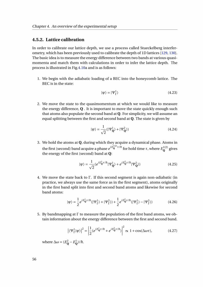
Chapter 4. An overview of the experimental setup
4.5.2. Lattice calibration
In order to calibrate our lattice depth, we use a process called Stueckelberg interfer-ometry, which has been previously used to calibrate the depth of 1D lattices [129, 130].The basic idea is to measure the energy difference between two bands at various quasi-momenta and match them with calculations in order to infer the lattice depth. Theprocess is illustrated in Fig.4.10a and is as follows:
1. We begin with the adiabatic loading of a BEC into the honeycomb lattice. TheBEC is in the state:
|ψ⟩ = |Ψ1Γ⟩ (4.23)
2. We move the state to the quasimomentum at which we would like to measurethe energy difference, Q . It is important to move the state quickly enough suchthat atoms also populate the second band at Q. For simplicity, we will assume anequal splitting between the first and second band at Q. The state is given by
|ψ⟩ = 1p2
(|Ψ1Q⟩+ |Ψ2
Q⟩) (4.24)
3. We hold the atoms at Q, during which they acquire a dynamical phase. Atoms in
the first (second) band acquire a phase e i E 1(2)Q τ/ħ for hold time τ, where E 1(2)
Q givesthe energy of the first (second) band at Q:
|ψ⟩ = 1p2
(e i E 1Qτ/ħ|Ψ1
Q⟩+e i E 2Qτ/ħ|Ψ2
Q⟩) (4.25)
4. We move the state back to Γ. If this second segment is again non-adiabatic (inpractice, we always use the same force as in the first segment), atoms originallyin the first band split into first and second band atoms and likewise for secondband atoms:
|ψ⟩ = 1
2e i E 1
Qτ/ħ(|Ψ1Γ⟩+ |Ψ2
Γ⟩)+1
2e i E 2
Qτ/ħ(|Ψ1Γ⟩− |Ψ2
Γ⟩) (4.26)
5. By bandmapping at Γ to measure the population of the first band atoms, we ob-tain information about the energy difference between the first and second band.
∣∣⟨Ψ1Γ|ψ⟩∣∣2 =
∣∣∣∣1
2(e i E 1
Qτ/ħ+e i E 2Qτ/ħ)
∣∣∣∣2
∝ 1+cos(∆ωτ), (4.27)
where ∆ω= (E 2Q −E 1
Q)/ħ.
56
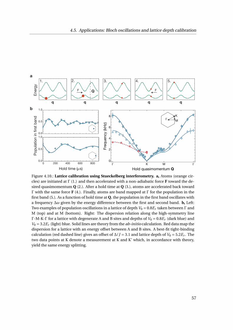
4.5. Applications: Bloch oscillations and lattice depth calibration
K M0
2
4
6
8
Freq
uenc
y (k
Hz)
Hold quasimomentum Q
MK
0.0
0.5
1.0
0 200 400 600 8000.0
0.5
1.0
Popu
latio
n in
firs
t ban
d
Hold time (µs)
a
b
Ener
gy
q
F
q
Q
F
1. 2. 3. 4. 5.
q
Figure 4.10.: Lattice calibration using Stueckelberg interferometry. a, Atoms (orange cir-cles) are initiated at Γ (1.) and then accelerated with a non-adiabatic force F toward the de-sired quasimomentum Q (2.). After a hold time at Q (3.), atoms are accelerated back towardΓ with the same force F (4.). Finally, atoms are band mapped at Γ for the population in thefirst band (5.). As a function of hold time at Q, the population in the first band oscillates witha frequency ∆ω given by the energy difference between the first and second band. b, Left:Two examples of population oscillations in a lattice of depth V0 = 0.8Er taken between Γ andM (top) and at M (bottom). Right: The dispersion relation along the high-symmetry lineΓ-M-K-Γ for a lattice with degenerate A and B sites and depths of V0 = 0.8Er (dark blue) andV0 = 3.2Er (light) blue. Solid lines are theory from the ab-initio calculation. Red data map thedispersion for a lattice with an energy offset between A and B sites. A best-fit tight-bindingcalculation (red dashed line) gives an offset of ∆/J = 3.1 and lattice depth of V0 = 5.2Er . Thetwo data points at K denote a measurement at K and K’ which, in accordance with theory,yield the same energy splitting.
57
Chapter 4. An overview of the experimental setup
Hence, as illustrated in the left panel Fig. 4.10b, by changing the hold time τ, we ob-tain an oscillation in the population of the first band. The contrast of the oscillationdepends on the splitting between bands, with a 50/50 splitting yielding the maximumcontrast. We, however, are more interested in the frequency of the oscillation, whichreveals the energy difference between the first and second bands. By repeating thismeasurement sequence at various Q, we obtain a map of the dispersion relation overthe entire Brillouin zone (right panel of Fig. 4.10b). We can then calculate the disper-sion at various lattice depths, choose the dispersion that best fits our data, and there-fore, find our lattice depth. The solid theory lines in Fig. 4.10b are ab-initio calculationsat lattice depths that match our data the best by eye. In practice, when calibrating ourlattice each day before experimental runs, we measure only the Γ point.
Due to the vanishing energy gap at the Dirac point, it becomes progressively moredifficult to measure the energy difference in the vicinity of the K point. The problemis two-fold: the period of the oscillations becomes longer, necessitating longer holdtimes near K, while dynamical instabilities due to our weakly-interacting BEC limit thelifetime of the condensate [131–133]. We can, however, open a gap at the Dirac point byadding an energy-offset between A and B sites of the lattice. This allows us to measurethe energy difference between first and second bands at K (red data in Fig. 4.10b). Byfitting our data to a tight-binding model, we obtain an energy-offset of ∆/J = 3.1.
58

Chapter 5.
Measuring the Berry phase
In this chapter, we measure the geometric phase acquired by a particle adiabaticallyencircling a Dirac point. We begin by drawing an analogy between our experiment andthe Aharonov-Bohm effect [134], in which electrons encircle an infinitely long solenoidof magnetic flux and experience a phase shift in their interference pattern despite al-ways traversing a region of zero magnetic field. We then present the spin-echo interfer-ometry used to perform our measurements in Sec. 5.2.1, followed by a brief descriptionof experimental parameters in Sec. 5.2.2. Although the interferometric sequence ide-ally yields only the geometric phase, technical imperfections preclude complete can-cellation of dynamical phases and contribute to our experimental uncertainty; theseissues are discussed in Sec. 5.2.3. Finally, we conclude with experimental results inSec. 5.3. A more thorough account of the contents of this chapter can be found inRef. [78].
5.1. An analogy with the Aharonov-Bohm effect
The Aharonov-Bohm effect clearly demonstrated the importance of electromagneticpotentials. Previously, in classical mechanics, these potentials were mainly consideredas convenient tools for formulating electromagnetic fields, with no physically mean-ingful consequences due to their gauge-dependence [134]. However, as we saw inSec. 2.3, a gauge-dependent quantity, such as the Berry connection, can yield gauge-invariant quantities under certain circumstances, such as the Berry phase. In fact, theAharonov-Bohm effect, which preceded Berry’s paper by more than two decades, canbe elegantly formulated in terms of Berry connections, phases, and curvatures [23,135].
In the Aharonov-Bohm effect, the particle encircling a confined magnetic field ac-quires a phase shift due to the electromagnetic vector potential. In Berry-terms, thevector potential is analogous to the Berry connection. Accordingly, the phase acquiredby the particles when traversing a closed path is simply the line-integral of the Berryconnection, i.e., the Berry phase. Just as the magnetic field is the curl of the electro-magnetic vector potential, the Berry curvature is the curl of the Berry connection. Sincethe Berry phase can be equivalently expressed as an area integral of the Berry curva-
59
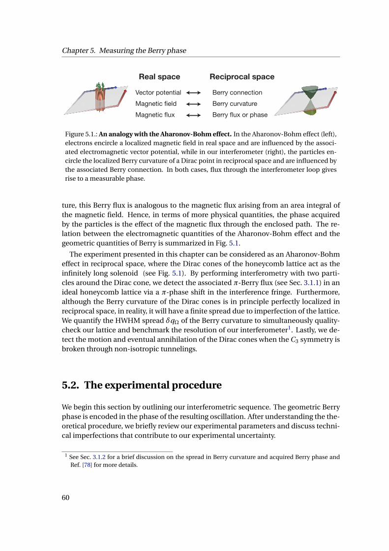
Chapter 5. Measuring the Berry phase
Real space Reciprocal space
Vector potentialMagnetic fieldMagnetic flux
Berry connectionBerry curvatureBerry flux or phase
Figure 5.1.: An analogy with the Aharonov-Bohm effect. In the Aharonov-Bohm effect (left),electrons encircle a localized magnetic field in real space and are influenced by the associ-ated electromagnetic vector potential, while in our interferometer (right), the particles en-circle the localized Berry curvature of a Dirac point in reciprocal space and are influenced bythe associated Berry connection. In both cases, flux through the interferometer loop givesrise to a measurable phase.
ture, this Berry flux is analogous to the magnetic flux arising from an area integral ofthe magnetic field. Hence, in terms of more physical quantities, the phase acquiredby the particles is the effect of the magnetic flux through the enclosed path. The re-lation between the electromagnetic quantities of the Aharonov-Bohm effect and thegeometric quantities of Berry is summarized in Fig. 5.1.
The experiment presented in this chapter can be considered as an Aharonov-Bohmeffect in reciprocal space, where the Dirac cones of the honeycomb lattice act as theinfinitely long solenoid (see Fig. 5.1). By performing interferometry with two parti-cles around the Dirac cone, we detect the associated π-Berry flux (see Sec. 3.1.1) in anideal honeycomb lattice via a π-phase shift in the interference fringe. Furthermore,although the Berry curvature of the Dirac cones is in principle perfectly localized inreciprocal space, in reality, it will have a finite spread due to imperfection of the lattice.We quantify the HWHM spread δqΩ of the Berry curvature to simultaneously quality-check our lattice and benchmark the resolution of our interferometer1. Lastly, we de-tect the motion and eventual annihilation of the Dirac cones when the C3 symmetry isbroken through non-isotropic tunnelings.
5.2. The experimental procedure
We begin this section by outlining our interferometric sequence. The geometric Berryphase is encoded in the phase of the resulting oscillation. After understanding the the-oretical procedure, we briefly review our experimental parameters and discuss techni-cal imperfections that contribute to our experimental uncertainty.
1 See Sec. 3.1.2 for a brief discussion on the spread in Berry curvature and acquired Berry phase andRef. [78] for more details.
60

5.2. The experimental procedure
2. 3. 4. 5.1. 6.
π/2, 0 π, 0 π/2, φMWDuration and phase of MW pulse
time
ϕ
qy
qx
Figure 5.2.: The interferometric procedure. The hexagons indicate the first Brillouin zoneand the spin state |↑⟩ (|↓⟩) is denoted by the red (blue) circle. After initializing the atoms in|↑⟩ (1), aπ/2-pulse is applied to create a superposition of states |↑⟩ and |↓⟩ (2). This is followedby an evolution time of τ= 0.8 ms (3). Next, a π-pulse is applied to swap the spin-states (4).After another evolution segment of time τ (5), a π/2-pulse is applied with variable phaseφMW to close the interferometer.
5.2.1. The sequence
To measure the geometric phase acquired by two states encircling the Dirac cone, weperform a spin-echo sequence inspired by Ref. [136]. We utilize hyperfine states withopposite magnetic moment as spin states |↑⟩ and |↓⟩. The procedure is as follows (seeFig. 5.2):
1. The sequence begins with a BEC of 87Rb in state |ψ⟩ = |↑⟩ at the center of theBrillouin zone.
2. We apply a π/2 microwave-pulse to create an equal superposition of |↑⟩ and |↓⟩.In general, the rotation matrix in the basis of the |↑⟩ and |↓⟩ states can be ex-pressed as
R(θ,φ) = cos(θ/2) −e iφ sin(θ/2)
e−iφ sin(θ/2) cos(θ/2),
(5.1)
where θ is the rotation angle andφ is the phase of the microwave pulse. The stateis now
|ψ⟩ = 1p2
(|↑⟩+ |↓⟩) (5.2)
3. We allow |ψ⟩ to evolve for a time τ in the presence of a lattice acceleration and amagnetic field gradient. These hyperfine states have opposite magnetic momentand therefore experience a force in opposite directions along the x-axis due tothe magnetic field gradient. In combination with the spin-independent lattice
61
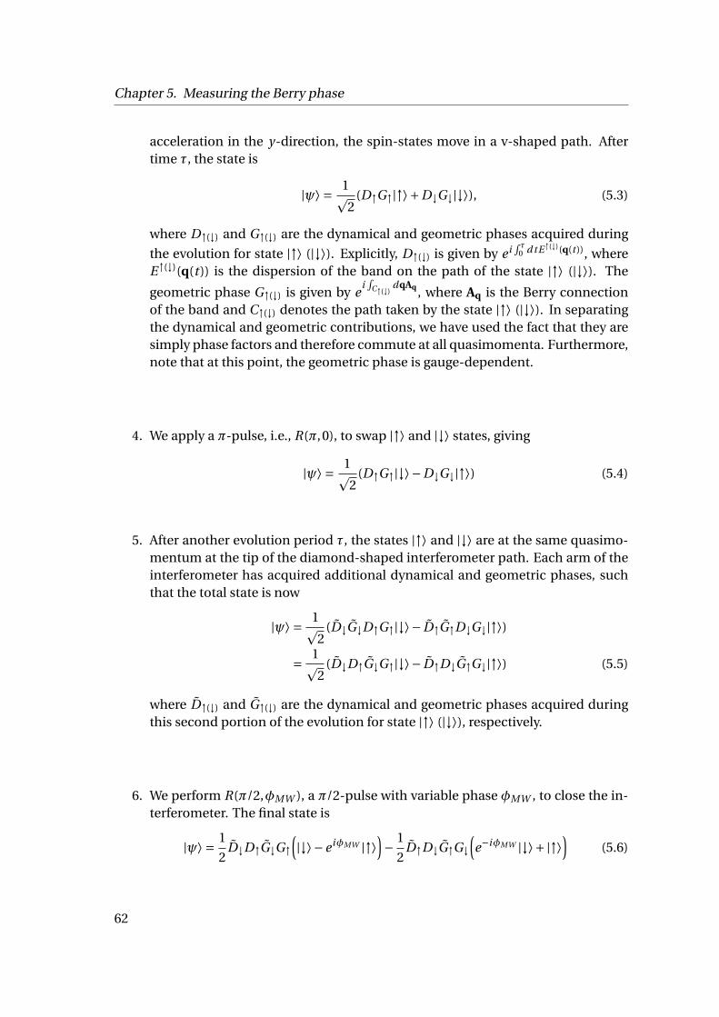
Chapter 5. Measuring the Berry phase
acceleration in the y-direction, the spin-states move in a v-shaped path. Aftertime τ, the state is
|ψ⟩ = 1p2
(D↑G↑|↑⟩+D↓G↓|↓⟩), (5.3)
where D↑(↓) and G↑(↓) are the dynamical and geometric phases acquired during
the evolution for state |↑⟩ (|↓⟩). Explicitly, D↑(↓) is given by e i∫ τ
0 d tE↑(↓)(q(t )), whereE↑(↓)(q(t )) is the dispersion of the band on the path of the state |↑⟩ (|↓⟩). The
geometric phase G↑(↓) is given by ei∫
C↑(↓)dqAq , where Aq is the Berry connection
of the band and C↑(↓) denotes the path taken by the state |↑⟩ (|↓⟩). In separatingthe dynamical and geometric contributions, we have used the fact that they aresimply phase factors and therefore commute at all quasimomenta. Furthermore,note that at this point, the geometric phase is gauge-dependent.
4. We apply a π-pulse, i.e., R(π,0), to swap |↑⟩ and |↓⟩ states, giving
|ψ⟩ = 1p2
(D↑G↑|↓⟩−D↓G↓|↑⟩) (5.4)
5. After another evolution period τ, the states |↑⟩ and |↓⟩ are at the same quasimo-mentum at the tip of the diamond-shaped interferometer path. Each arm of theinterferometer has acquired additional dynamical and geometric phases, suchthat the total state is now
|ψ⟩ = 1p2
(D↓G↓D↑G↑|↓⟩− D↑G↑D↓G↓|↑⟩)
= 1p2
(D↓D↑G↓G↑|↓⟩− D↑D↓G↑G↓|↑⟩) (5.5)
where D↑(↓) and G↑(↓) are the dynamical and geometric phases acquired duringthis second portion of the evolution for state |↑⟩ (|↓⟩), respectively.
6. We perform R(π/2,φMW ), a π/2-pulse with variable phase φMW , to close the in-terferometer. The final state is
|ψ⟩ = 1
2D↓D↑G↓G↑
(|↓⟩−e iφMW |↑⟩
)− 1
2D↑D↓G↑G↓
(e−iφMW |↓⟩+ |↑⟩
)(5.6)
62
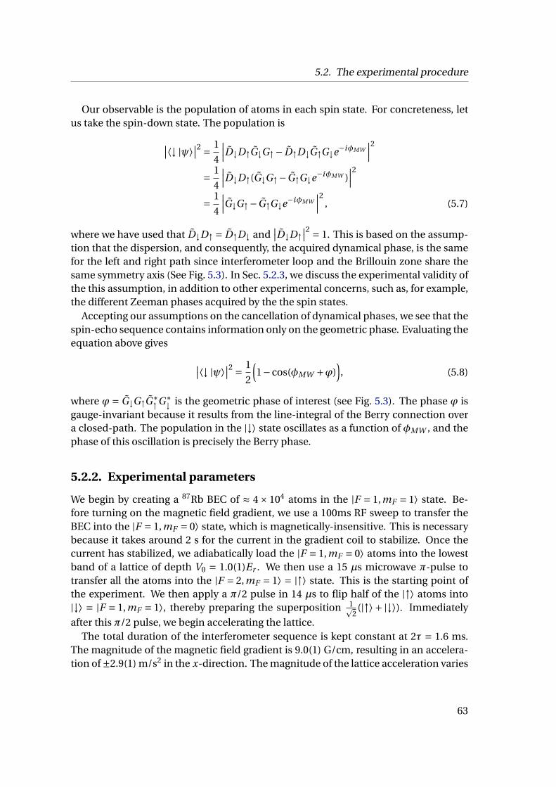
5.2. The experimental procedure
Our observable is the population of atoms in each spin state. For concreteness, letus take the spin-down state. The population is
∣∣⟨↓ |ψ⟩∣∣2 = 1
4
∣∣∣D↓D↑G↓G↑− D↑D↓G↑G↓e−iφMW
∣∣∣2
= 1
4
∣∣∣D↓D↑(G↓G↑−G↑G↓e−iφMW )∣∣∣2
= 1
4
∣∣∣G↓G↑−G↑G↓e−iφMW
∣∣∣2, (5.7)
where we have used that D↓D↑ = D↑D↓ and∣∣D↓D↑
∣∣2 = 1. This is based on the assump-tion that the dispersion, and consequently, the acquired dynamical phase, is the samefor the left and right path since interferometer loop and the Brillouin zone share thesame symmetry axis (See Fig. 5.3). In Sec. 5.2.3, we discuss the experimental validity ofthe this assumption, in addition to other experimental concerns, such as, for example,the different Zeeman phases acquired by the the spin states.
Accepting our assumptions on the cancellation of dynamical phases, we see that thespin-echo sequence contains information only on the geometric phase. Evaluating theequation above gives
∣∣⟨↓ |ψ⟩∣∣2 = 1
2
(1−cos(φMW +ϕ)
), (5.8)
where ϕ = G↓G↑G∗↑G∗
↓ is the geometric phase of interest (see Fig. 5.3). The phase ϕ isgauge-invariant because it results from the line-integral of the Berry connection overa closed-path. The population in the |↓⟩ state oscillates as a function of φMW , and thephase of this oscillation is precisely the Berry phase.
5.2.2. Experimental parameters
We begin by creating a 87Rb BEC of ≈ 4× 10⁴ atoms in the |F = 1,mF = 1⟩ state. Be-fore turning on the magnetic field gradient, we use a 100ms RF sweep to transfer theBEC into the |F = 1,mF = 0⟩ state, which is magnetically-insensitive. This is necessarybecause it takes around 2 s for the current in the gradient coil to stabilize. Once thecurrent has stabilized, we adiabatically load the |F = 1,mF = 0⟩ atoms into the lowestband of a lattice of depth V0 = 1.0(1)Er . We then use a 15 µs microwave π-pulse totransfer all the atoms into the |F = 2,mF = 1⟩ = |↑⟩ state. This is the starting point ofthe experiment. We then apply a π/2 pulse in 14 µs to flip half of the |↑⟩ atoms into|↓⟩ = |F = 1,mF = 1⟩, thereby preparing the superposition 1p
2(|↑⟩ + |↓⟩). Immediately
after this π/2 pulse, we begin accelerating the lattice.The total duration of the interferometer sequence is kept constant at 2τ = 1.6 ms.
The magnitude of the magnetic field gradient is 9.0(1) G/cm, resulting in an accelera-tion of ±2.9(1) m/s2 in the x-direction. The magnitude of the lattice acceleration varies
63
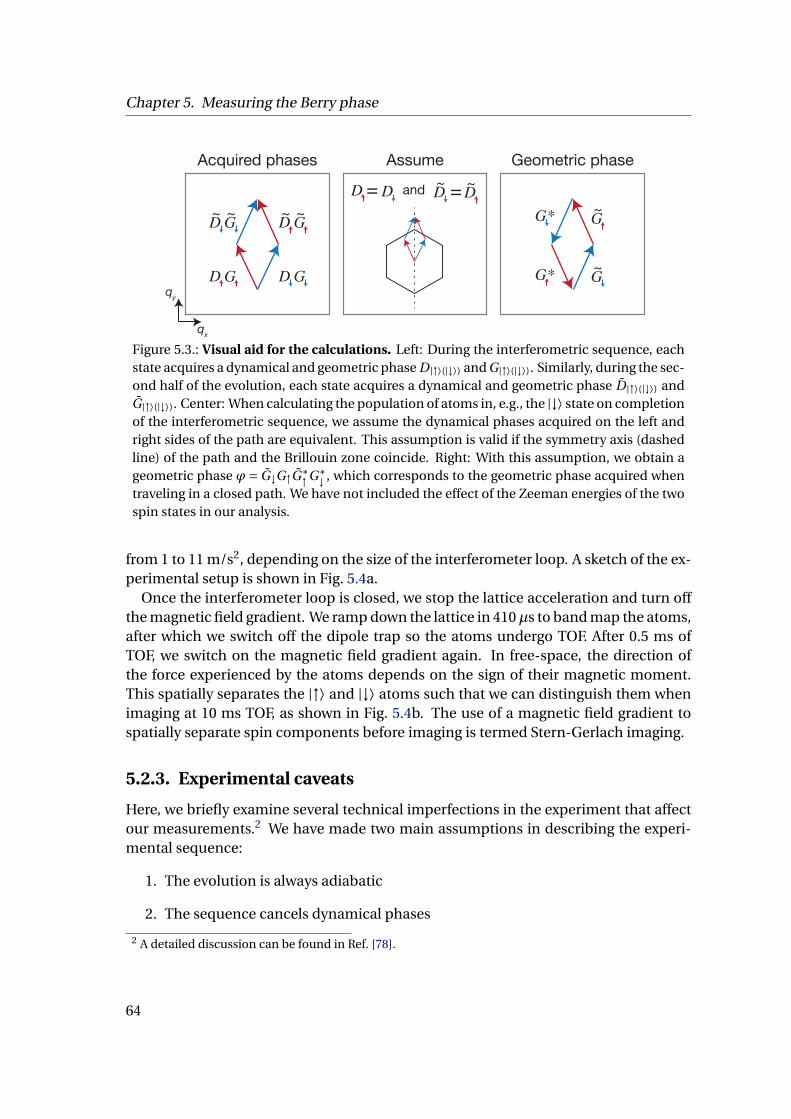
Chapter 5. Measuring the Berry phase
GD GD
G~
D~
G~
D~
Acquired phases Assume Geometric phase
G*
G*
G~
G~
D=D
qx
qy
D~D
~ =and
Figure 5.3.: Visual aid for the calculations. Left: During the interferometric sequence, eachstate acquires a dynamical and geometric phase D |↑⟩(|↓⟩) and G|↑⟩(|↓⟩). Similarly, during the sec-ond half of the evolution, each state acquires a dynamical and geometric phase D |↑⟩(|↓⟩) andG|↑⟩(|↓⟩). Center: When calculating the population of atoms in, e.g., the |↓⟩ state on completionof the interferometric sequence, we assume the dynamical phases acquired on the left andright sides of the path are equivalent. This assumption is valid if the symmetry axis (dashedline) of the path and the Brillouin zone coincide. Right: With this assumption, we obtain ageometric phase ϕ= G↓G↑G∗
↑G∗↓ , which corresponds to the geometric phase acquired when
traveling in a closed path. We have not included the effect of the Zeeman energies of the twospin states in our analysis.
from 1 to 11 m/s2, depending on the size of the interferometer loop. A sketch of the ex-perimental setup is shown in Fig. 5.4a.
Once the interferometer loop is closed, we stop the lattice acceleration and turn offthe magnetic field gradient. We ramp down the lattice in 410µs to band map the atoms,after which we switch off the dipole trap so the atoms undergo TOF. After 0.5 ms ofTOF, we switch on the magnetic field gradient again. In free-space, the direction ofthe force experienced by the atoms depends on the sign of their magnetic moment.This spatially separates the |↑⟩ and |↓⟩ atoms such that we can distinguish them whenimaging at 10 ms TOF, as shown in Fig. 5.4b. The use of a magnetic field gradient tospatially separate spin components before imaging is termed Stern-Gerlach imaging.
5.2.3. Experimental caveats
Here, we briefly examine several technical imperfections in the experiment that affectour measurements.2 We have made two main assumptions in describing the experi-mental sequence:
1. The evolution is always adiabatic
2. The sequence cancels dynamical phases
2 A detailed discussion can be found in Ref. [78].
64
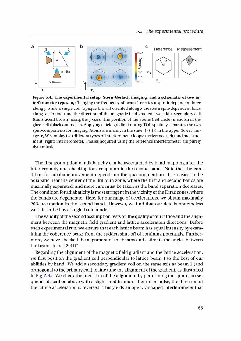
5.2. The experimental procedure
b
y
x
qy
qx
a
ωL+δω
B
Reference Measurement
y
x
Density (a.u)
min
max
ϕ
c
1
23
Figure 5.4.: The experimental setup, Stern-Gerlach imaging, and a schematic of two in-terferometer types. a, Changing the frequency of beam 1 creates a spin-independent forcealong y while a single coil (opaque brown) oriented along x creates a spin-dependent forcealong x. To fine-tune the direction of the magnetic field gradient, we add a secondary coil(translucent brown) along the y-axis. The position of the atoms (red circle) is shown in theglass cell (black outline). b, Applying a field gradient during TOF spatially separates the twospin-components for imaging. Atoms are mainly in the state |↑⟩ (|↓⟩) in the upper (lower) im-age. c, We employ two different types of interferometer loops: a reference (left) and measure-ment (right) interferometer. Phases acquired using the reference interferometer are purelydynamical.
The first assumption of adiabaticity can be ascertained by band mapping after theinterferomety and checking for occupation in the second band. Note that the con-dition for adiabatic movement depends on the quasimomentum. It is easiest to beadiabatic near the center of the Brillouin zone, where the first and second bands aremaximally separated, and more care must be taken as the band separation decreases.The condition for adiabaticity is most stringent in the vicinity of the Dirac cones, wherethe bands are degenerate. Here, for our range of accelerations, we obtain maximally20% occupation in the second band. However, we find that our data is nonethelesswell-described by a single-band model.
The validity of the second assumption rests on the quality of our lattice and the align-ment between the magnetic field gradient and lattice acceleration directions. Beforeeach experimental run, we ensure that each lattice beam has equal intensity by exam-ining the coherence peaks from the sudden shut-off of confining potentials. Further-more, we have checked the alignment of the beams and estimate the angles betweenthe beams to be 120(1).
Regarding the alignment of the magnetic field gradient and the lattice acceleration,we first position the gradient coil perpendicular to lattice beam 1 to the best of ourabilities by hand. We add a secondary gradient coil on the same axis as beam 1 (andorthogonal to the primary coil) to fine tune the alignment of the gradient, as illustratedin Fig. 5.4a. We check the precision of the alignment by performing the spin-echo se-quence described above with a slight modification–after the π-pulse, the direction ofthe lattice acceleration is reversed. This yields an open, v-shaped interferometer that
65
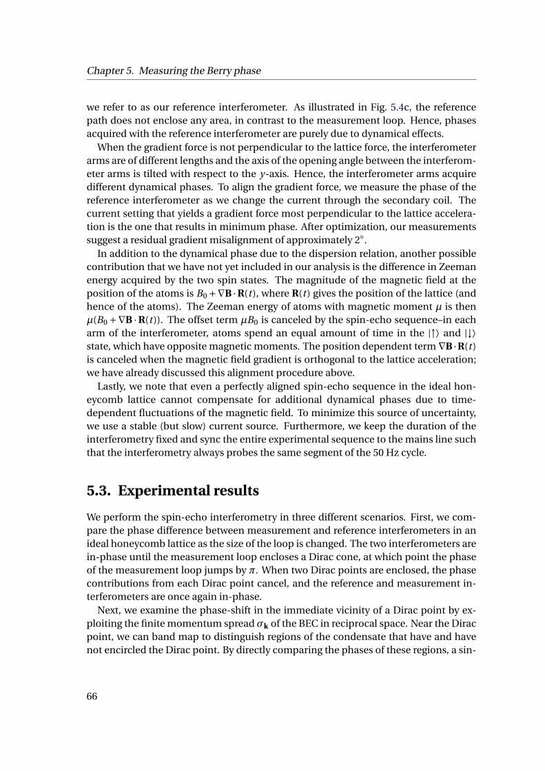
Chapter 5. Measuring the Berry phase
we refer to as our reference interferometer. As illustrated in Fig. 5.4c, the referencepath does not enclose any area, in contrast to the measurement loop. Hence, phasesacquired with the reference interferometer are purely due to dynamical effects.
When the gradient force is not perpendicular to the lattice force, the interferometerarms are of different lengths and the axis of the opening angle between the interferom-eter arms is tilted with respect to the y-axis. Hence, the interferometer arms acquiredifferent dynamical phases. To align the gradient force, we measure the phase of thereference interferometer as we change the current through the secondary coil. Thecurrent setting that yields a gradient force most perpendicular to the lattice accelera-tion is the one that results in minimum phase. After optimization, our measurementssuggest a residual gradient misalignment of approximately 2.
In addition to the dynamical phase due to the dispersion relation, another possiblecontribution that we have not yet included in our analysis is the difference in Zeemanenergy acquired by the two spin states. The magnitude of the magnetic field at theposition of the atoms is B0 +∇B ·R(t ), where R(t ) gives the position of the lattice (andhence of the atoms). The Zeeman energy of atoms with magnetic moment µ is thenµ(B0 +∇B ·R(t )). The offset term µB0 is canceled by the spin-echo sequence–in eacharm of the interferometer, atoms spend an equal amount of time in the |↑⟩ and |↓⟩state, which have opposite magnetic moments. The position dependent term ∇B ·R(t )is canceled when the magnetic field gradient is orthogonal to the lattice acceleration;we have already discussed this alignment procedure above.
Lastly, we note that even a perfectly aligned spin-echo sequence in the ideal hon-eycomb lattice cannot compensate for additional dynamical phases due to time-dependent fluctuations of the magnetic field. To minimize this source of uncertainty,we use a stable (but slow) current source. Furthermore, we keep the duration of theinterferometry fixed and sync the entire experimental sequence to the mains line suchthat the interferometry always probes the same segment of the 50 Hz cycle.
5.3. Experimental results
We perform the spin-echo interferometry in three different scenarios. First, we com-pare the phase difference between measurement and reference interferometers in anideal honeycomb lattice as the size of the loop is changed. The two interferometers arein-phase until the measurement loop encloses a Dirac cone, at which point the phaseof the measurement loop jumps by π. When two Dirac points are enclosed, the phasecontributions from each Dirac point cancel, and the reference and measurement in-terferometers are once again in-phase.
Next, we examine the phase-shift in the immediate vicinity of a Dirac point by ex-ploiting the finite momentum spreadσk of the BEC in reciprocal space. Near the Diracpoint, we can band map to distinguish regions of the condensate that have and havenot encircled the Dirac point. By directly comparing the phases of these regions, a sin-
66
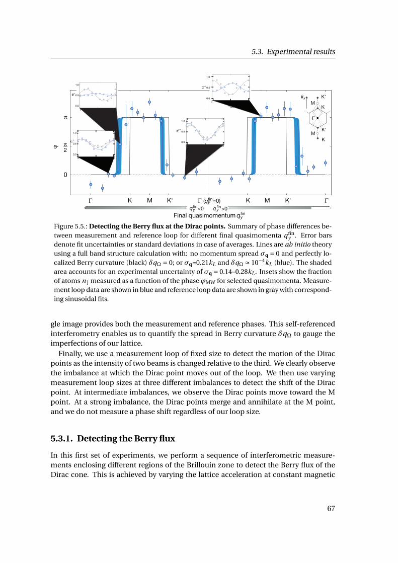
5.3. Experimental results
Γ (qy =0)Γ K'MK K M K' Γ
Final quasimomentum qyfin
ϕ
0
π2
π
↑n
ϕMW
0.0
1.0
0.5
0 2ππ
↑n
0.0
1.0
0.5
ϕMW
0 2ππ
Γ
K’
KM
ky
fin
K’
KM
qyfin<0 qy
fin>0
↑ n
0.0
1.0
0.5
0 2ππϕMW
↑ n
ϕMW
0.0
1.0
0 2ππ
0.5
Figure 5.5.: Detecting the Berry flux at the Dirac points. Summary of phase differences be-tween measurement and reference loop for different final quasimomenta qfin
y . Error barsdenote fit uncertainties or standard deviations in case of averages. Lines are ab initio theoryusing a full band structure calculation with: no momentum spread σq = 0 and perfectly lo-calized Berry curvature (black) δqΩ = 0; or σq=0.21kL and δqΩ ' 10−4kL (blue). The shadedarea accounts for an experimental uncertainty of σq = 0.14–0.28kL . Insets show the fractionof atoms n↓ measured as a function of the phase ϕMW for selected quasimomenta. Measure-ment loop data are shown in blue and reference loop data are shown in gray with correspond-ing sinusoidal fits.
gle image provides both the measurement and reference phases. This self-referencedinterferometry enables us to quantify the spread in Berry curvature δqΩ to gauge theimperfections of our lattice.
Finally, we use a measurement loop of fixed size to detect the motion of the Diracpoints as the intensity of two beams is changed relative to the third. We clearly observethe imbalance at which the Dirac point moves out of the loop. We then use varyingmeasurement loop sizes at three different imbalances to detect the shift of the Diracpoint. At intermediate imbalances, we observe the Dirac points move toward the Mpoint. At a strong imbalance, the Dirac points merge and annihilate at the M point,and we do not measure a phase shift regardless of our loop size.
5.3.1. Detecting the Berry flux
In this first set of experiments, we perform a sequence of interferometric measure-ments enclosing different regions of the Brillouin zone to detect the Berry flux of theDirac cone. This is achieved by varying the lattice acceleration at constant magnetic
67
Chapter 5. Measuring the Berry phase
field gradient to control the final quasimomentum qfiny (qfin
x = 0) of the diamond-shaped measurement loop. The resulting phase differences between measurementand reference loops are shown in Fig. 5.5. When the measurement loop does not en-close a Dirac point, measurement and reference loops are in-phase. When one Diracpoint is enclosed in the measurement loop, we observe a phase difference of ϕ ' π.When two Dirac points are enclosed, the phase difference is again zero, since the πcontribution to the phase difference from the first Dirac point is canceled by the −πcontribution from the second Dirac point.3
In comparison to the single-particle theory line, the position of the phase jump isshifted in our measurements. This discrepancy is primarily due to the finite momen-tum spread σq of our weakly-interacting BEC. When this is accounted for, we find verygood agreement with theory . The position of the phase jump shifts because atomsin different parts of the cloud sample slightly different paths in reciprocal space. Forinstance, atoms near the top of the cloud will reach the Dirac cone before atoms nearthe bottom of the cloud. We measure a phase jump only once the measurement loopfor at least half the atoms have enclosed the Dirac point. While the momentum spreadaffects the position of the phase jumps, it does not limit their sharpness. In fact, wewill next exploit the momentum spread to improve the precision of our measurementin the vicinity of the Dirac point.
5.3.2. Self-referenced interferometry near the Dirac point
To minimize systematic errors and improve our measurement precision, we performself-referenced interferometry close to the Dirac points. Due to the finite momentumspread, atoms near the Dirac point will be "sliced" by the Brillouin zone into sectionsthat have or have not crossed the edge of the Brillouin zone, as illustrated in Fig. 5.6a.These three slices will be band mapped onto three different corners of the first Brillouinzone, allowing us to separately analyze the phase of each slice. Combining the phasesof these three slices ϕL , ϕR and ϕB to
ϕ= (ϕL +ϕR )/2−ϕB , (5.9)
eliminates the need for a separate reference measurement and significantly reducesthe sensitivity to drifts in the experiment.
The phase ϕ exhibits a sudden jump from 0 to π as the atoms cross the edge of theband (see Fig. 5.6b). The position of the phase jump is in excellent agreement with anumerical calculation including an initial momentum spread of σq = 0.15(1)kL , con-sistent with an independent TOF measurement. Remarkably, the phase jump occurswithin a very small quasimomentum range of < 0.01kL , and an arctangent fit to the ex-
3 We know that, theoretically, the two inequivalent Dirac points contribute Berry phases of ±π. How-ever, we cannot experimentally determine whether the Dirac points have the same or opposite signbecause we cannot differentiate between a phase shift of 2π or zero.
68
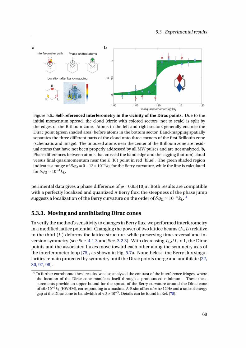
5.3. Experimental results
1.201.00 1.05 1.10 1.15finFinal quasimomentum qy /kL
π2
π
ϕ
0
K
K’
Interferometer path
R L
Phase-shifted atoms
Location after band-mapping
RL
B
B
ba
Figure 5.6.: Self-referenced interferometry in the vicinity of the Dirac points. Due to theinitial momentum spread, the cloud (circle with colored sectors, not to scale) is split bythe edges of the Brillouin zone. Atoms in the left and right sectors generally encircle theDirac point (green shaded area) before atoms in the bottom sector. Band-mapping spatiallyseparates the three different parts of the cloud onto three corners of the first Brillouin zone(schematic and image). The unboxed atoms near the center of the Brillouin zone are resid-ual atoms that have not been properly addressed by all MW pulses and are not analyzed. b,Phase differences between atoms that crossed the band edge and the lagging (bottom) cloudversus final quasimomentum near the K (K’) point in red (blue). The green shaded regionindicates a range of δqΩ = 0−12×10−4kL for the Berry curvature, while the line is calculatedfor δqΩ ' 10−4kL .
perimental data gives a phase difference of ϕ=0.95(10)π. Both results are compatiblewith a perfectly localized and quantized π Berry flux; the steepness of the phase jumpsuggests a localization of the Berry curvature on the order of δqΩ ' 10−4kL . 4
5.3.3. Moving and annihilating Dirac cones
To verify the method’s sensitivity to changes in Berry flux, we performed interferometryin a modified lattice potential. Changing the power of two lattice beams (I3, I2) relativeto the third (I1) deforms the lattice structure, while preserving time-reversal and in-version symmetry (see Sec. 4.1.3 and Sec. 3.2.3). With decreasing I3,2/I1 < 1, the Diracpoints and the associated fluxes move toward each other along the symmetry axis ofthe interferometer loop [75], as shown in Fig. 5.7a. Nonetheless, the Berry flux singu-larities remain protected by symmetry until the Dirac points merge and annihilate [22,30, 97, 98].
4 To further corroborate these results, we also analyzed the contrast of the interference fringes, wherethe location of the Dirac cone manifests itself through a pronounced minimum. These mea-surements provide an upper bound for the spread of the Berry curvature around the Dirac coneof <6×10⁻⁴kL (HWHM), corresponding to a maximal A-B site offset of ≈ h×12 Hz and a ratio of energygap at the Dirac cone to bandwidth of < 3×10⁻³. Details can be found in Ref. [78].
69
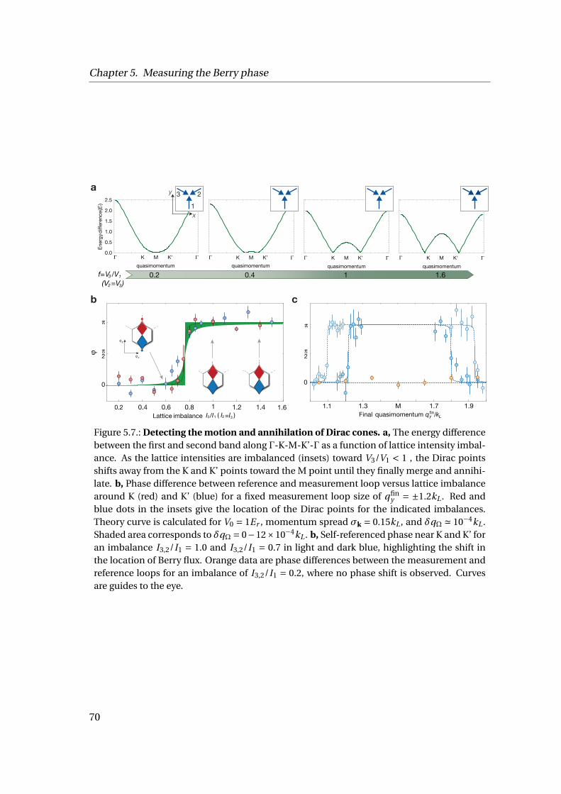
Chapter 5. Measuring the Berry phase
1.1 1.3 M 1.7 1.9fin/kL
π
0
π2
Final quasimomentum qy
y
q x
q
ϕ
Lattice imbalance I3/I1 ( I2 =I )3
0
π2
π
0.2 0.4 0.6 1.2 1.40.8 1 1.6
cb
MK K’Γ Γ
quasimomentumMK K’Γ Γ
quasimomentum
0.0
0.5
1.0
1.5
2.0
2.5
Ener
gydi
ffere
nce(
E r)
quasimomentumMK K’Γ Γ MK K’Γ Γ
quasimomentumV /V3 1
(V =V )2 3
1 1.60.2 0.4f=
a
x
y
123
Figure 5.7.: Detecting the motion and annihilation of Dirac cones. a, The energy differencebetween the first and second band along Γ-K-M-K’-Γ as a function of lattice intensity imbal-ance. As the lattice intensities are imbalanced (insets) toward V3/V1 < 1 , the Dirac pointsshifts away from the K and K’ points toward the M point until they finally merge and annihi-late. b, Phase difference between reference and measurement loop versus lattice imbalancearound K (red) and K’ (blue) for a fixed measurement loop size of qfin
y = ±1.2kL . Red andblue dots in the insets give the location of the Dirac points for the indicated imbalances.Theory curve is calculated for V0 = 1Er , momentum spread σk = 0.15kL , and δqΩ ' 10−4kL .Shaded area corresponds to δqΩ = 0−12×10−4kL . b, Self-referenced phase near K and K’ foran imbalance I3,2/I1 = 1.0 and I3,2/I1 = 0.7 in light and dark blue, highlighting the shift inthe location of Berry flux. Orange data are phase differences between the measurement andreference loops for an imbalance of I3,2/I1 = 0.2, where no phase shift is observed. Curvesare guides to the eye.
70
5.3. Experimental results
By using a fixed measurement loop that encloses one Dirac point in the intensity-balanced case, we can measure the change of the geometric phase as we imbalancethe lattice beam intensities. As shown in Fig. 5.7, the measured Berry phases drop fromπ to 0 as the Dirac point moves out of the loop, in very good agreement with ab initiocalculations.
To precisely map the location of the Berry flux in the imbalanced lattice, we again usethe self-referenced interferometry. As shown in Fig. 5.7, imbalancing the lattice by de-creasing I3,2/I1 narrows the range of final quasimomenta for which the interferometerencloses a single π flux, thereby shifting both the upward and downward phase jumpstowards the M point. For a stronger imbalance (I3,2/I1=0.2), the two Dirac points haveannihilated, and hence no phase jump is observed for any loop size.
71

Chapter 6.
Bloch state tomography with Wilsonlines
In this chapter, we realize strong-gradient dynamics described by Wilson lines to mapout the geometric structure of the s-bands. We begin by describing the two ways inwhich Wilson lines can be used to characterize band structures. First, the eigenvaluesof Wilson lines transporting a state by a reciprocal lattice vector G can be used to for-mulate the Z2 invariant [77, 90, 137]. Secondly, in certain situations, the form of theWilson line can be simplified and, when measured in the basis of the band eigenstates,enables a complete map of the cell-periodic Bloch functions over the entire Brillouinzone. Although the primary focus of the chapter is on the band tomography, the sameexperimental techniques can also be used to obtain the eigenvalues.
In Sec. 6.2, we introduce a Bloch sphere formalism which enables us to parametrizethe cell-periodic Bloch function |un
q ⟩ at any quasimomentum q in terms of two angles,θq and φq, that are directly related to the elements of the Wilson line. After describingthe experimental procedures used to measure these two angles, we move onto someexperimental details in Sec. 6.3. We note the experimental parameters necessary toreach the strong-gradient regime where dynamics are described by two-band Wilsonlines and consider the validity of our two-band approximation. Next, we explain ourdata analysis techniques before presenting our experimental results in Sec. 6.4. Unsur-prisingly, in addition to mapping the cell-periodic Bloch functions, our measurementsof θq and φq also reflect certain real-space attributes of the lattice.
Finally, in Sec. 6.5, we examine the situation more commonly considered in solidstate theory and obtain the eigenvalues of a Wilson line transporting by a single recip-rocal lattice vector. Since measuring θq and φq is equivalent to measuring the Wilsonline elements in the basis of the band eigenstates, we are able to reconstruct such aWilson line and extract its eigenvalues. We find the same eigenvalues for two differentlattice configurations with different geometric attributes, corroborating the fact thatthese eigenvalues reflect the topological structure of the bands.
73
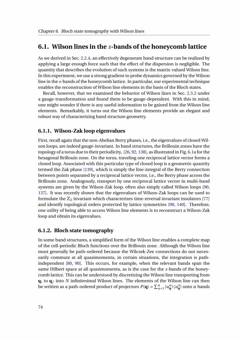
Chapter 6. Bloch state tomography with Wilson lines
6.1. Wilson lines in the s-bands of the honeycomb lattice
As we derived in Sec. 2.2.4, an effectively degenerate band structure can be realized byapplying a large enough force such that the effect of the dispersion is negligible. Thequantity that describes the evolution of such systems is the matrix-valued Wilson line.In this experiment, we use a strong gradient to probe dynamics governed by the Wilsonline in the s-bands of the honeycomb lattice. In particular, our experimental techniqueenables the reconstruction of Wilson line elements in the basis of the Bloch states.
Recall, however, that we examined the behavior of Wilson lines in Sec. 2.3.2 undera gauge-transformation and found them to be gauge-dependent. With this in mind,one might wonder if there is any useful information to be gained from the Wilson lineelements. Remarkably, it turns out the Wilson line elements provide an elegant androbust way of characterizing band structure geometry.
6.1.1. Wilson-Zak loop eigenvalues
First, recall again that the non-Abelian Berry phases, i.e., the eigenvalues of closed Wil-son loops, are indeed gauge-invariant. In band structures, the Brillouin zones have thetopology of a torus due to their periodicity, [26, 92, 138], as illustrated in Fig. 6.1a for thehexagonal Brillouin zone. On the torus, traveling one reciprocal lattice vector forms aclosed loop. Associated with this particular type of closed loop is a geometric quantitytermed the Zak phase [139], which is simply the line-integral of the Berry connectionbetween points separated by a reciprocal lattice vector, i.e., the Berry phase across theBrillouin zone. Analogously, transport by one reciprocal lattice vector in multi-bandsystems are given by the Wilson-Zak loop, often also simply called Wilson loops [90,137]. It was recently shown that the eigenvalues of Wilson-Zak loops can be used toformulate the Z2 invariant which characterizes time-reversal invariant insulators [77]and identify topological orders protected by lattice symmetries [90, 140]. Therefore,one utility of being able to access Wilson line elements is to reconstruct a Wilson-Zakloop and obtain its eigenvalues.
6.1.2. Bloch state tomography
In some band structures, a simplified form of the Wilson line enables a complete mapof the cell-periodic Bloch functions over the Brillouin zone. Although the Wilson linemust generally be path-ordered because the Wilczek-Zee connections do not neces-sarily commute at all quasimomenta, in certain situations, the integration is path-independent [80, 90]. This occurs, for example, when the relevant bands span thesame Hilbert space at all quasimomenta, as is the case for the s-bands of the honey-comb lattice. This can be understood by discretizing the Wilson line transporting fromqi to q f into N infinitesimal Wilson lines. The elements of the Wilson line can thenbe written as a path-ordered product of projectors P (q) =∑α
n=1 |unq ⟩⟨un
q | onto α bands
74

6.1. Wilson lines in the s-bands of the honeycomb lattice
sandwiched between the cell-periodic states at the initial and final quasimomenta [90]:
W mnq1→qN
= ⟨unqN
|N∏
i=1P (qi )|um
q1⟩ (6.1)
Since the projection operator reduces to identity, P (q) = ∑αn=1 |un
q ⟩⟨unq | = 1, when the
bands span the same Hilbert subspace at each quasimomentum, the Wilson line re-duces to
W mnq1→qN
= ⟨unqN
|umq1⟩. (6.2)
Consequently, the elements of the Wilson line are simply given by the projection of thefinal cell-periodic Bloch state onto the initial cell-periodic Bloch state. Accordingly, ifwe set a reference quasimomenta Q and compare the cell-periodic Bloch states at allother quasimomenta to the states at Q, we can map the structure of the eigenstatesover the entire Brillouin zone.
An alternative, more physical way of understanding this simplified form of the Wil-son line elements is to consider the dynamics in real-space. If the gradient F · r is thelargest energy scale of the system, it dominates the dynamics and the time-evolution
operator, i.e., the Wilson line, after time τ is simply eiħτF·r.
Since the application of a force F for period τ results in a change in quasimomentumgiven by Fτ/ħ [89], the Wilson line can be equivalently written as
Wqi→q f = e i∆q·r, (6.3)
where∆q = q f −qi is the change in quasimomentum. Here, we see that the Wilson lineis simply the quasimomentum translation operator. Measuring this Wilson line in thebasis of the band eigenstates yields
⟨Φnq f|Wqi→q f |Φm
qi⟩ = ⟨un
q f|e i∆q·r|um
qi⟩ = ⟨un
q f|um
qi⟩, (6.4)
since |Φmq ⟩ = e i q·r|um
q ⟩. Hence, we arrive at the same conclusion as our purely math-ematical analysis above–when the relevant bands span the same Hilbert space at allquasimomenta, the Wilson line elements enable a comparison between cell-periodicBloch states at any two quasimomenta.
In the remainder of the chapter, we primarily focus on exploiting Eq. 6.2 or Eq. 6.4 fora tomography of the cell-periodic Bloch states. It is important to note, however, thatthe experimental technique is applicable even in more complex scenarios when thebands do not fulfill a completeness relation. In this case, there is no obvious relationbetween the Wilson line elements and the cell-periodic Bloch states, but we can stillobtain information about the band structure through the eigenvalues of Wilson-Zakloops. In Sec. 6.5, we reconstruct a single Wilson-Zak loop and extract its eigenval-
75
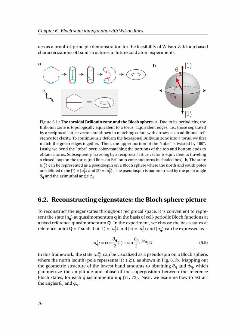
Chapter 6. Bloch state tomography with Wilson lines
ues as a proof-of-principle demonstration for the feasibility of Wilson-Zak loop basedcharacterizations of band structures in future cold atom experiments.
θq
φq
a b
=qy
qx
Figure 6.1.: The toroidal Brillouin zone and the Bloch sphere. a, Due to its periodicity, theBrillouin zone is topologically equivalent to a torus. Equivalent edges, i.e., those separatedby a reciprocal lattice vector, are shown in matching colors with arrows as an additional ref-erence for clarity. To continuously deform the hexagonal Brillouin zone into a torus, we firstmatch the green edges together. Then, the upper portion of the “tube" is twisted by 180.Lastly, we bend the “tube" over, color-matching the portions of the top and bottom ends toobtain a torus. Subsequently, traveling by a reciprocal lattice vector is equivalent to travelinga closed loop on the torus (red lines on Brillouin zone and torus in shaded box). b, The state|un
q ⟩ can be represented as a pseudospin on a Bloch sphere where the north and south polesare defined to be |1⟩ = |u1
Γ⟩ and |2⟩ = |u2Γ⟩. The pseudospin is parametrized by the polar angle
θq and the azimuthal angle φq.
6.2. Reconstructing eigenstates: the Bloch sphere picture
To reconstruct the eigenstates throughout reciprocal space, it is convenient to repre-sent the state |u1
q⟩ at quasimomentum q in the basis of cell-periodic Bloch functions ata fixed reference quasimomentum Q. In the experiment, we choose the basis states atreference point Q = Γ such that |1⟩ = |u1
Γ⟩ and |2⟩ = |u2Γ⟩ and |u1
q⟩ can be expressed as
|u1q⟩ = cos
θq
2|1⟩+ sin
θq
2e iφq |2⟩. (6.5)
In this framework, the state |unq ⟩ can be visualized as a pseudospin on a Bloch sphere,
where the north (south) pole represents |1⟩ (|2⟩), as shown in Fig. 6.1b. Mapping outthe geometric structure of the lowest band amounts to obtaining θq and φq, whichparametrize the amplitude and phase of the superposition between the referenceBloch states, for each quasimomentum q [71, 72]. Next, we examine how to extractthe angles θq and φq.
76
6.2. Reconstructing eigenstates: the Bloch sphere picture
6.2.1. Extracting the polar angle θq
The polar angle can be obtained from the quantity∣∣∣⟨u1q|1⟩
∣∣∣= ∣∣∣∣cosθq
2
∣∣∣∣⇒ θq = 2arccos
∣∣∣⟨u1q|1⟩
∣∣∣= 2arccos∣∣∣W 11
Γ→q
∣∣∣ (6.6)
Hence, the element∣∣∣W 11
Γ→q
∣∣∣ of the Wilson line directly gives θq. To experimentally mea-
sure this element, we perform the following steps:
1. Prepare the initial state as the Bloch state of the first band at quasimomentum Γ
|Φ1Γ⟩ (6.7)
2. Evolve the the state to a final quasimomentum q by applying a suitable force.The evolved state is given by
WΓ→q|Φ1Γ⟩ (6.8)
3. Band map at final quasimomentum q. This yields the population in the firstband, given by: ∣∣∣⟨Φ1
q|WΓ→q|Φ1Γ⟩
∣∣∣2 =∣∣∣W 11
Γ→q
∣∣∣2(6.9)
Taking the square-root of the population in the first band after transport yields theabsolute-value of W 11
Γ→q and, therefore, θq.
6.2.2. Extracting the azimuthal angle φq
The relative phase φq can be expressed as1
φq = Arg[⟨u1q|1⟩]−Arg[⟨u1
q|2⟩]= Arg[W 11
Γ→q]−Arg[W 12Γ→q] (6.10)
1 From Eq. 6.5, we have
Arg[⟨1|u1q⟩] = Arg[cos
θq
2] = 0
Arg[⟨2|u1q⟩] = Arg[e−iφq sin
θq
2] =−φq
Hence, φq = Arg[⟨1|u1q⟩]−Arg[⟨2|u1
q⟩].
77
Chapter 6. Bloch state tomography with Wilson lines
Therefore, to access φq, we must access the phases of the Wilson line elements. Thisis experimentally accomplished via a process similar to Ramsey interferometry. Thegeneral idea is to first create a superposition state with a time-varying phase at quasi-momentum Γ. In the basis of the band eigenstates at Γ, the superposition state is:
|ΨΓ⟩ =(
|α|∣∣β∣∣e i∆ωt
), (6.11)
where |α|2 (∣∣β∣∣2) denotes the population in first (second) band and ∆ωt is the phase-
difference between the basis states at time t . We then rapidly transport this state to thedesired quasimomentum q. Assuming the Wilson line operator has form
WΓ→q =W 11 W 12
W 21 W 22
,
the resulting state at the desired quasimomentum q is
|Ψq⟩ = WΓ→q|ΨΓ⟩ =(|α|W 11 + ∣∣β∣∣W 12e i∆ωt
|α|W 21 + ∣∣β∣∣W 22e i∆ωt
). (6.12)
The resulting population in the first band at q is given by∣∣∣⟨Φ1q|Ψq⟩
∣∣∣2 = ∣∣αW 11∣∣+ ∣∣βW 12
∣∣+2
∣∣αβW 11W 12∣∣cos
(∆ωt +Arg[W 11]−Arg[W 12]
). (6.13)
We see that the population oscillates as a function of time. The azimuthal phase φq isencoded in the phase of the oscillation.
The experimental procedure, as illustrated in Fig. 6.2a, is as follows:
1. The superposition state with time-varying phase is created by rapidly transport-ing atoms initialized in the first band at Γ−G by one reciprocal lattice vector.
2. We then hold the state at Γ for variable time. Written in the basis of the bandeigenstates at Γ, the state |ΨΓ⟩ after a hold time t is:
|ΨΓ⟩ = 1
2
(1p
3e i∆ωt
), (6.14)
where ħ∆ω= E 2Γ−E 1
Γ is the energy separation between the first and second bandat Γ.
3. We rapidly transport this superposition state to quasimomentum q, yielding the
78
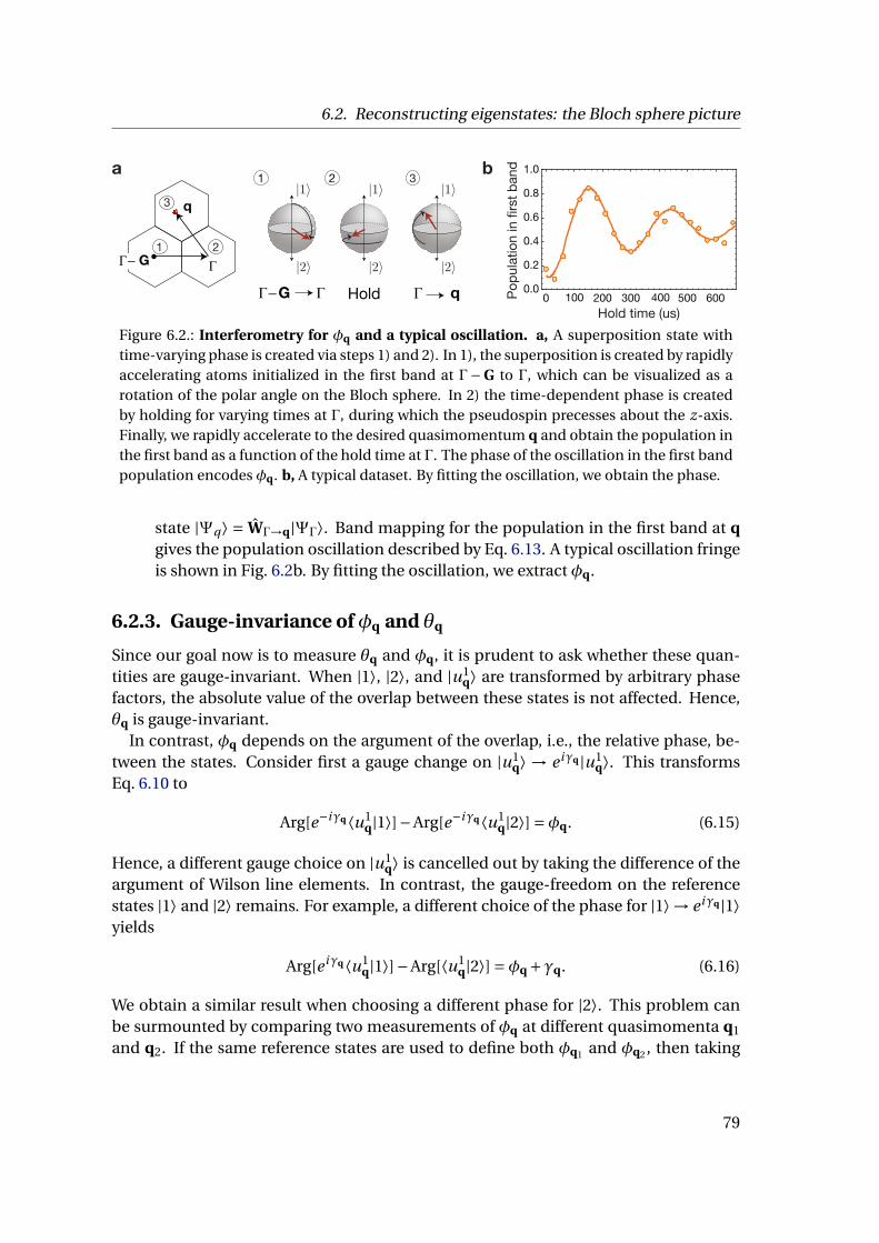
6.2. Reconstructing eigenstates: the Bloch sphere picture
G
q
1 2
HoldG q
a b
0 100 200 300 400 500 6000.0
0.2
0.4
0.6
0.8
1.0
Popu
latio
n in
firs
t ban
d
Hold time (us)
3
21
3
Figure 6.2.: Interferometry for φq and a typical oscillation. a, A superposition state withtime-varying phase is created via steps 1) and 2). In 1), the superposition is created by rapidlyaccelerating atoms initialized in the first band at Γ− G to Γ, which can be visualized as arotation of the polar angle on the Bloch sphere. In 2) the time-dependent phase is createdby holding for varying times at Γ, during which the pseudospin precesses about the z-axis.Finally, we rapidly accelerate to the desired quasimomentum q and obtain the population inthe first band as a function of the hold time at Γ. The phase of the oscillation in the first bandpopulation encodes φq. b, A typical dataset. By fitting the oscillation, we obtain the phase.
state |Ψq⟩ = WΓ→q|ΨΓ⟩. Band mapping for the population in the first band at qgives the population oscillation described by Eq. 6.13. A typical oscillation fringeis shown in Fig. 6.2b. By fitting the oscillation, we extract φq.
6.2.3. Gauge-invariance of φq and θq
Since our goal now is to measure θq and φq, it is prudent to ask whether these quan-tities are gauge-invariant. When |1⟩, |2⟩, and |u1
q⟩ are transformed by arbitrary phasefactors, the absolute value of the overlap between these states is not affected. Hence,θq is gauge-invariant.
In contrast, φq depends on the argument of the overlap, i.e., the relative phase, be-tween the states. Consider first a gauge change on |u1
q⟩ → e iγq |u1q⟩. This transforms
Eq. 6.10 to
Arg[e−iγq⟨u1q|1⟩]−Arg[e−iγq⟨u1
q|2⟩] =φq. (6.15)
Hence, a different gauge choice on |u1q⟩ is cancelled out by taking the difference of the
argument of Wilson line elements. In contrast, the gauge-freedom on the referencestates |1⟩ and |2⟩ remains. For example, a different choice of the phase for |1⟩→ e iγq |1⟩yields
Arg[e iγq⟨u1q|1⟩]−Arg[⟨u1
q|2⟩] =φq +γq. (6.16)
We obtain a similar result when choosing a different phase for |2⟩. This problem canbe surmounted by comparing two measurements of φq at different quasimomenta q1
and q2. If the same reference states are used to define both φq1 and φq2 , then taking
79

Chapter 6. Bloch state tomography with Wilson lines
the difference φq1 −φq2 cancels out the gauge-freedom of the reference states.In fact, a comparison of φq’s at different quasimomenta already implicitly occurs
in our measurement of φq, a detail we neglected to mention in Sec. 6.2.2. This detailoccurs in the creation of the superposition state using a Wilson line WΓ−G→Γ transport-ing a state from Γ−G to Γ. A more accurate description of the superposition state inEq. 6.11 would be
|ΨΓ⟩ =(
|α|∣∣β∣∣e i (∆ωt+φ′)
), (6.17)
where |α| = ∣∣W 11Γ−G→Γ
∣∣ ,∣∣β∣∣= ∣∣W 21
Γ−G→Γ∣∣ , and
φ′ = Arg[W 21Γ−G→Γ]−Arg[W 11
Γ−G→Γ]
= ⟨2|u1Γ⟩−⟨1|u1
Γ⟩=−φΓ (6.18)
The superposition state, by nature of its creation, already contains a gauge-dependentphase. Consequently, the phase of the oscillation in the first band population we mea-sure is actually
φq −φΓ, (6.19)
which is a gauge-invariant quantity, although both φq and φΓ are gauge-dependent.That we actually measure a difference between phases is of no concern since we areonly interested in how φq changes as we move around the Brillouin zone. In otherwords,φΓ can be thought of as a reference phase, just as |1⟩ and |2⟩ are reference states.
6.3. Experimental details
In this section, we describe the experimental parameters required to reach the regimewhere the dynamics are well-described by two-band Wilson lines. From Sec. 2.2.4, weknow that the applied force needs to be large and here, we determine the requiredmagnitude. Furthermore, since our band structure of course has an infinite amountof bands, we examine the validity of the two-band approximation. We conclude thesection with a description of our data analysis techniques.
6.3.1. Experimental parameters
Each experimental sequence begins by adiabatically loading a BEC of 87Rb into thelowest band of a lattice of depth V0 = 5.2(1)Er at quasimomentum q = Γ. At this depth,the combined width ε ≈ h× 3 kHz of the lowest two bands is much smaller than the
80
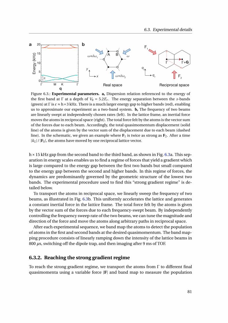
6.3. Experimental details
+1
+2
x
y
A B
Real space
F1
F2
qx
qy
+G
Reciprocal space
a b
Γ M K Γ0
5
10
15
20
Ener
gy (k
Hz)
q
ε
Figure 6.3.: Experimental parameters. a, Dispersion relation referenced to the energy ofthe first band at Γ at a depth of V0 = 5.2Er . The energy separation between the s-bands(green) at Γ is ε≈ h×3 kHz. There is a much larger energy gap to higher bands (red), enablingus to approximate our experiment as a two-band system. b, The frequency of two beamsare linearly swept at independently chosen rates (left). In the lattice frame, an inertial forcemoves the atoms in reciprocal space (right). The total force felt by the atoms is the vector sumof the forces due to each beam. Accordingly, the total quasimomentum displacement (solidline) of the atoms is given by the vector sum of the displacement due to each beam (dashedline). In the schematic, we given an example where F1 is twice as strong as F2. After a time|kL |/ |F1|, the atoms have moved by one reciprocal lattice vector.
h×15 kHz gap from the second band to the third band, as shown in Fig. 6.3a. This sep-aration in energy scales enables us to find a regime of forces that yield a gradient whichis large compared to the energy gap between the first two bands but small comparedto the energy gap between the second and higher bands. In this regime of forces, thedynamics are predominantly governed by the geometric structure of the lowest twobands. The experimental procedure used to find this “strong gradient regime" is de-tailed below.
To transport the atoms in reciprocal space, we linearly sweep the frequency of twobeams, as illustrated in Fig. 6.3b. This uniformly accelerates the lattice and generatesa constant inertial force in the lattice frame. The total force felt by the atoms is givenby the vector sum of the forces due to each frequency-swept beam. By independentlycontrolling the frequency sweep rate of the two beams, we can tune the magnitude anddirection of the force and move the atoms along arbitrary paths in reciprocal space.
After each experimental sequence, we band map the atoms to detect the populationof atoms in the first and second bands at the desired quasimomentum. The band map-ping procedure consists of linearly ramping down the intensity of the lattice beams in800 µs, switching off the dipole trap, and then imaging after 9 ms of TOF.
6.3.2. Reaching the strong gradient regime
To reach the strong gradient regime, we transport the atoms from Γ to different finalquasimomenta using a variable force |F| and band map to measure the population
81
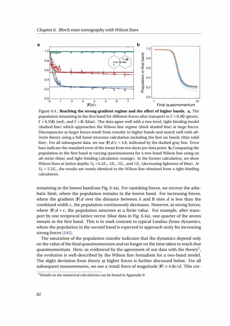
Chapter 6. Bloch state tomography with Wilson lines
0.0
0.2
0.4
0.6
0.8
1.0
Final quasimomentum
Popu
latio
n in
firs
t ban
d
Γ M
a1.0
0.0
0.2
0.4
0.6
0.8
5 6 70 1 2 3 4|F|d/ε
+G
b
Figure 6.4.: Reaching the strong-gradient regime and the effect of higher bands. a, Thepopulation remaining in the first band for different forces after transport to Γ+0.2G (green),Γ+0.55G (red), and Γ+G (blue). The data agree well with a two-level, tight-binding model(dashed line) which approaches the Wilson line regime (thick shaded line) at large forces.Discrepancies at larger forces result from transfer to higher bands and match well with ab-initio theory using a full band structure calculation including the first six bands (thin solidline). For all subsequent data, we use |F|d/ε = 4.8, indicated by the dashed gray line. Errorbars indicate the standard error of the mean from ten shots per data point. b, Comparing thepopulation in the first band at varying quasimomenta for a two-band Wilson line using anab-initio (blue) and tight-binding calculation (orange). In the former calculation, we showWilson lines at lattice depths V0 =5.2Er , 3Er , 2Er , and 1Er (decreasing lightness of blue). AtV0 = 5.2Er , the results are nearly identical to the Wilson line obtained from a tight-bindingcalculation.
remaining in the lowest band(see Fig. 6.4a). For vanishing forces, we recover the adia-batic limit, where the population remains in the lowest band. For increasing forces,where the gradient |F|d over the distance between A and B sites d is less than thecombined width ε, the population continuously decreases. However, at strong forces,where |F|d > ε, the population saturates at a finite value. For example, after trans-port by one reciprocal lattice vector (blue data in Fig. 6.4a), one quarter of the atomsremain in the first band. This is in stark contrast to typical Landau-Zener dynamics,where the population in the second band is expected to approach unity for increasingstrong forces [141].
The saturation of the population transfer indicates that the dynamics depend onlyon the value of the final quasimomentum and no longer on the time taken to reach thatquasimomentum. Here, as evidenced by the agreement of our data with the theory2,the evolution is well-described by the Wilson line formalism for a two-band model.The slight deviation from theory at higher forces is further discussed below. For allsubsequent measurements, we use a (total) force of magnitude |F| ≈ 4.8ε/d . This cor-
2Details on the numerical calculations can be found in Appendix B.
82

6.3. Experimental details
responds to an acceleration of 250 m/s2 and a Bloch period of ≈ 42 µs.
6.3.3. The effect of higher bands
Previously, we claimed that the system is well-described by a two-band model. How-ever, we already see deviations of the data from the two-band tight-binding theory inFig. 6.4a at larger forces. In this section, we determine whether this deviation is pri-marily due to the tight-binding approximation or the two-band approximation. To thisend, we compare two-band Wilson lines, i.e., neglecting the dispersion of the bands,from an ab-initio and tight-binding calculation in Fig. 6.4b. While deviations are signif-icant at shallow lattices, they are already small at a lattice depth of V0 = 5.2Er . Hence,we can conclude that it is not the tight-binding assumption, but rather the two-bandassumption at fault. This conclusion is further corroborated by the excellent agree-ment between data and theory when six bands are taken into account (solid lines inFig. 6.4a).
True two-band Wilson lines can only be realized by reaching the infinite gradientlimit for the two lowest bands while remaining adiabatic with respect to higher bands.This is of course not experimentally possible due to the presence of higher bands. Ingeneral, the choice of gradient strength is a compromise between realizing dynamicsthat are fast compared to the energy scale of the lowest two bands and minimizingexcitations into higher bands. We could, in principle, realize the two-band Wilson lineregime more precisely by increasing the lattice depth, which decreases the combinedwidth ε of the lowest two bands and increases the energy scale between the lowest twobands and higher bands. However, in the current work, the lattice depth was limitedby the band mapping technique. As the lattice depth is increased, it becomes moredifficult for the band mapping process to remain adiabatic with respect to ε.
6.3.4. Data analysis
ROI selection
To obtain the population of atoms in the first band, we identify regions of inter-est (ROIs) of first band and second band atoms. Example ROIs are depicted in Fig. 6.5afor atoms accelerated by approximately one reciprocal lattice vector. We count thenumber of atoms in the first band n1 and the atoms in the second zone n2. Subse-quently, the relative population in the first band is given by n1/(n1 +n2). Practically,“counting" the atoms means summing the pixel values within the specified regions ofinterest, i.e., the red circle for first band atoms (n1) and the six blue circles for secondband atoms (n2).
To obtain a quantitatively accurate fraction in the first band, we subtract from n1
the mean pixel value of the region enclosed by the dashed red circles. This accountsfor the hot background atoms. We do perform an additional background subtrac-
83
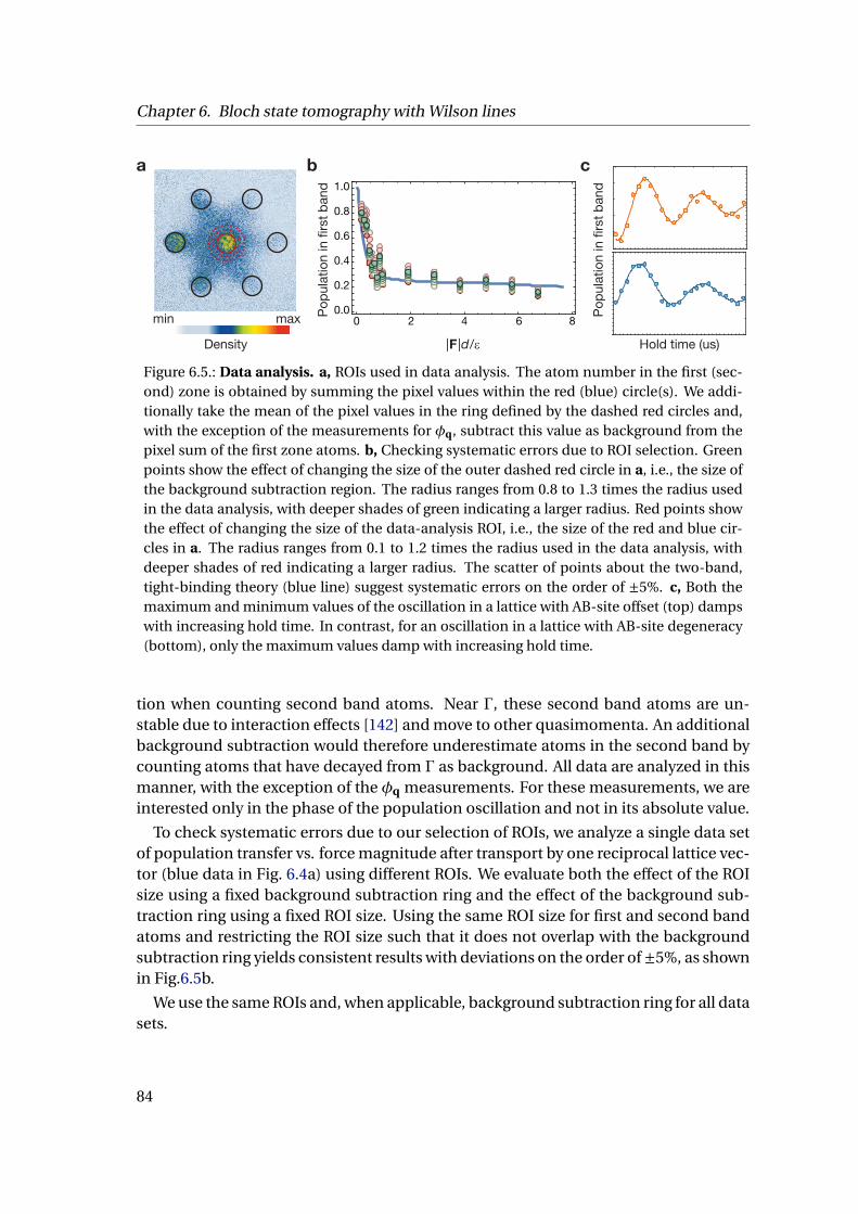
Chapter 6. Bloch state tomography with Wilson lines
a b
0 2 4 6 80.0
0.2
0.4
0.6
0.8
1.0
Popu
latio
n in
firs
t ban
d|F|d/ε
Popu
latio
n in
firs
t ban
d
Hold time (us)
c
Density
min max
Figure 6.5.: Data analysis. a, ROIs used in data analysis. The atom number in the first (sec-ond) zone is obtained by summing the pixel values within the red (blue) circle(s). We addi-tionally take the mean of the pixel values in the ring defined by the dashed red circles and,with the exception of the measurements for φq, subtract this value as background from thepixel sum of the first zone atoms. b, Checking systematic errors due to ROI selection. Greenpoints show the effect of changing the size of the outer dashed red circle in a, i.e., the size ofthe background subtraction region. The radius ranges from 0.8 to 1.3 times the radius usedin the data analysis, with deeper shades of green indicating a larger radius. Red points showthe effect of changing the size of the data-analysis ROI, i.e., the size of the red and blue cir-cles in a. The radius ranges from 0.1 to 1.2 times the radius used in the data analysis, withdeeper shades of red indicating a larger radius. The scatter of points about the two-band,tight-binding theory (blue line) suggest systematic errors on the order of ±5%. c, Both themaximum and minimum values of the oscillation in a lattice with AB-site offset (top) dampswith increasing hold time. In contrast, for an oscillation in a lattice with AB-site degeneracy(bottom), only the maximum values damp with increasing hold time.
tion when counting second band atoms. Near Γ, these second band atoms are un-stable due to interaction effects [142] and move to other quasimomenta. An additionalbackground subtraction would therefore underestimate atoms in the second band bycounting atoms that have decayed from Γ as background. All data are analyzed in thismanner, with the exception of the φq measurements. For these measurements, we areinterested only in the phase of the population oscillation and not in its absolute value.
To check systematic errors due to our selection of ROIs, we analyze a single data setof population transfer vs. force magnitude after transport by one reciprocal lattice vec-tor (blue data in Fig. 6.4a) using different ROIs. We evaluate both the effect of the ROIsize using a fixed background subtraction ring and the effect of the background sub-traction ring using a fixed ROI size. Using the same ROI size for first and second bandatoms and restricting the ROI size such that it does not overlap with the backgroundsubtraction ring yields consistent results with deviations on the order of±5%, as shownin Fig.6.5b.
We use the same ROIs and, when applicable, background subtraction ring for all datasets.
84
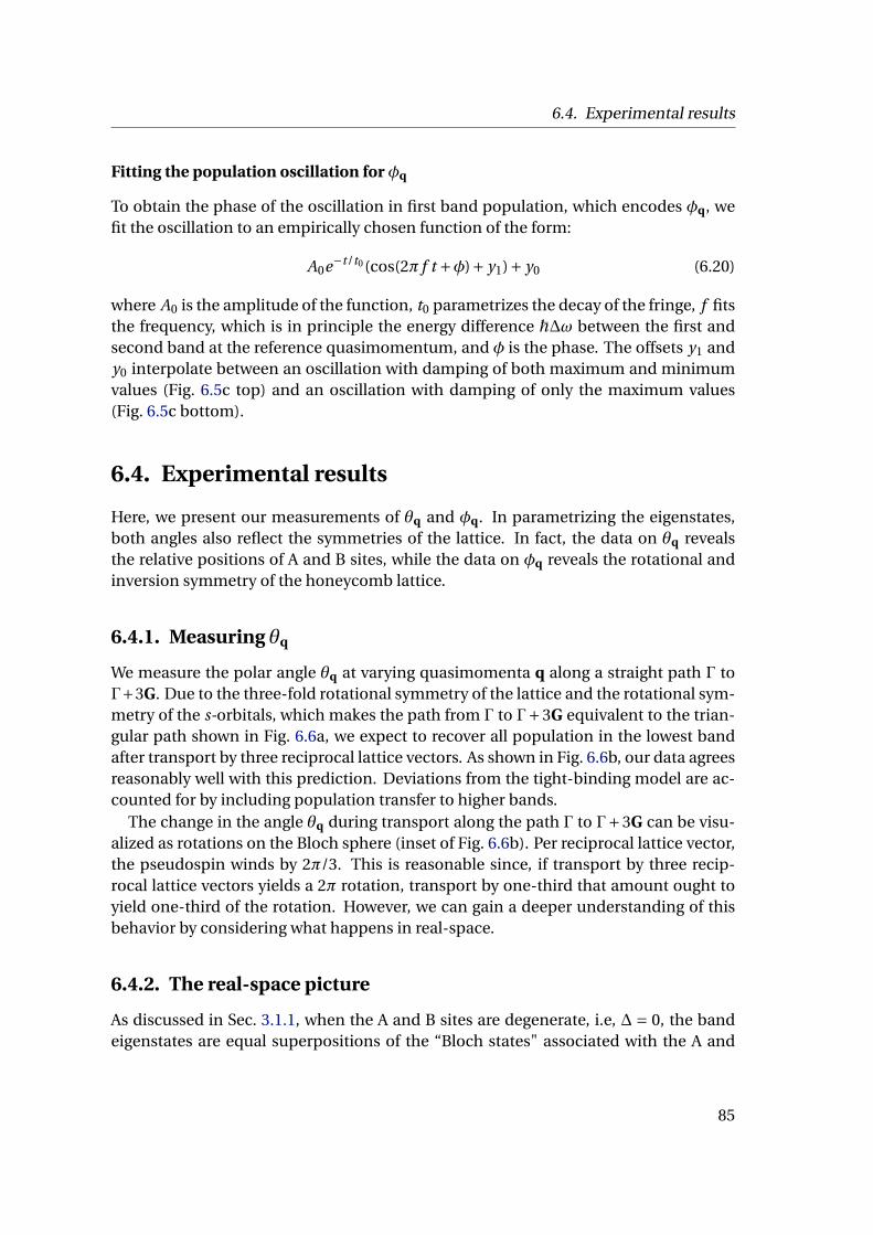
6.4. Experimental results
Fitting the population oscillation for φq
To obtain the phase of the oscillation in first band population, which encodes φq, wefit the oscillation to an empirically chosen function of the form:
A0e−t/t0 (cos(2π f t +φ)+ y1)+ y0 (6.20)
where A0 is the amplitude of the function, t0 parametrizes the decay of the fringe, f fitsthe frequency, which is in principle the energy difference ħ∆ω between the first andsecond band at the reference quasimomentum, and φ is the phase. The offsets y1 andy0 interpolate between an oscillation with damping of both maximum and minimumvalues (Fig. 6.5c top) and an oscillation with damping of only the maximum values(Fig. 6.5c bottom).
6.4. Experimental results
Here, we present our measurements of θq and φq. In parametrizing the eigenstates,both angles also reflect the symmetries of the lattice. In fact, the data on θq revealsthe relative positions of A and B sites, while the data on φq reveals the rotational andinversion symmetry of the honeycomb lattice.
6.4.1. Measuring θq
We measure the polar angle θq at varying quasimomenta q along a straight path Γ toΓ+3G. Due to the three-fold rotational symmetry of the lattice and the rotational sym-metry of the s-orbitals, which makes the path from Γ to Γ+3G equivalent to the trian-gular path shown in Fig. 6.6a, we expect to recover all population in the lowest bandafter transport by three reciprocal lattice vectors. As shown in Fig. 6.6b, our data agreesreasonably well with this prediction. Deviations from the tight-binding model are ac-counted for by including population transfer to higher bands.
The change in the angle θq during transport along the path Γ to Γ+3G can be visu-alized as rotations on the Bloch sphere (inset of Fig. 6.6b). Per reciprocal lattice vector,the pseudospin winds by 2π/3. This is reasonable since, if transport by three recip-rocal lattice vectors yields a 2π rotation, transport by one-third that amount ought toyield one-third of the rotation. However, we can gain a deeper understanding of thisbehavior by considering what happens in real-space.
6.4.2. The real-space picture
As discussed in Sec. 3.1.1, when the A and B sites are degenerate, i.e, ∆ = 0, the bandeigenstates are equal superpositions of the “Bloch states" associated with the A and
85
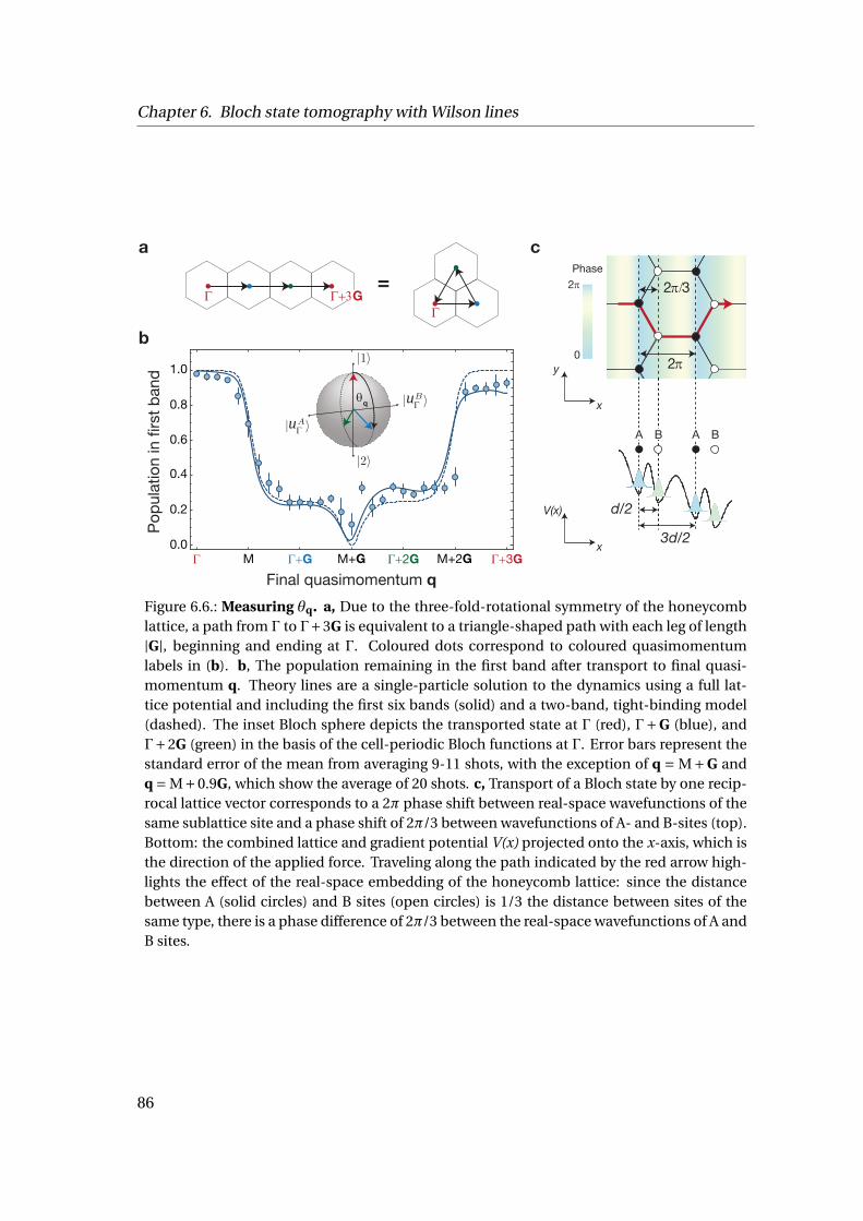
Chapter 6. Bloch state tomography with Wilson lines
M M+G M+2G0.0
0.2
0.4
0.6
0.8
1.0
Popu
latio
n in
firs
t ban
d
Final quasimomentum q
θq
Γ Γ+G Γ+2G Γ+3G
uΓ
uΓ
a
b
c
2π
2π/3
y
x
V(x)
x 3d/2
d/2
=Γ
ΓΓ+3G
0
2πPhase
A B A B
Figure 6.6.: Measuring θq. a, Due to the three-fold-rotational symmetry of the honeycomblattice, a path from Γ to Γ+3G is equivalent to a triangle-shaped path with each leg of length|G|, beginning and ending at Γ. Coloured dots correspond to coloured quasimomentumlabels in (b). b, The population remaining in the first band after transport to final quasi-momentum q. Theory lines are a single-particle solution to the dynamics using a full lat-tice potential and including the first six bands (solid) and a two-band, tight-binding model(dashed). The inset Bloch sphere depicts the transported state at Γ (red), Γ+G (blue), andΓ+2G (green) in the basis of the cell-periodic Bloch functions at Γ. Error bars represent thestandard error of the mean from averaging 9-11 shots, with the exception of q = M+G andq = M+0.9G, which show the average of 20 shots. c, Transport of a Bloch state by one recip-rocal lattice vector corresponds to a 2π phase shift between real-space wavefunctions of thesame sublattice site and a phase shift of 2π/3 between wavefunctions of A- and B-sites (top).Bottom: the combined lattice and gradient potential V(x) projected onto the x-axis, which isthe direction of the applied force. Traveling along the path indicated by the red arrow high-lights the effect of the real-space embedding of the honeycomb lattice: since the distancebetween A (solid circles) and B sites (open circles) is 1/3 the distance between sites of thesame type, there is a phase difference of 2π/3 between the real-space wavefunctions of A andB sites.
86
6.4. Experimental results
B sites, |ΦAq ⟩ and |ΦB
q ⟩3. Accordingly, the cell-periodic Bloch functions of the first andsecond band at Γ, which are our basis states |1⟩ and |2⟩, can also be expressed as equalsuperpositions of the “cell-periodic Bloch functions" associated with the A and B sites,|u AΓ ⟩ and |uB
Γ ⟩. These two states form an alternative set of basis states that can be rep-resented as an equatorial axis on the Bloch sphere. Furthermore, the state |un
q ⟩ must
rotate about this equatorial axis since |unq ⟩ remains an equal superposition of |u A
Γ ⟩ and
|uBΓ ⟩ throughout the evolution. Hence, as can be seen in the inset of Fig. 6.6b, the angle
θq, which parametrizes the superposition between states |1⟩ and |2⟩, also parametrizesthe phase between states |u A
Γ ⟩ and |uBΓ ⟩. Therefore, our aim now is to understand the
2π/3 rotation in θq by understanding why the states |u AΓ ⟩ and |uB
Γ ⟩ accumulate a phaseof 2π/3 when transporting by one reciprocal lattice vector.
In terms of states at Γ, the state |u1Γ+G⟩ can be represented as
|u1Γ+G⟩ = e i G·r|u1
Γ⟩= e i G·r 1p
2(|u A
Γ ⟩+ |uBΓ ⟩)
= e i G·r 1p2
(e−iΓ·r ∑rA
e iΓ·rA |wrA⟩+e−iΓ·r ∑rB
e iΓ·rB |wrB ⟩)
= e i G·r 1p2
(∑rA
|wrA⟩+∑rB
|wrB ⟩) (6.21)
In the equations above, we have explicitly expressed the Wilson line transporting fromΓ to Γ+G in its quasimomentum-translation operator form as e i G·r. In the second line,we write the state |u1
Γ⟩ in the basis of |u AΓ ⟩ and |uB
Γ ⟩. In the third line, we write the
quasimomentum-dependent state |u A (B)Γ ⟩ in terms of the real-space wavefunctions
|wrA (B)⟩ localized on the A (B) sites at positions rA (B). Lastly, we have used that thereal-space wavefunctions are eigenstates of the position operator, i.e., e−iΓ·r|wrA (B)⟩ =e−iΓ·rA (B) |wrA (B)⟩ [143]. From this last line, we see that the states |u A
Γ ⟩ and |uBΓ ⟩ are su-
perpositions of the real-space wavefunctions on the the A and B sites 4.
In the particular case of transport by one reciprocal lattice vector, we know that,since rA can be written as a sum of primitive lattice vectors, G ·rA = 2π. However, sincethe B-sites are displaced from the A-sites by δ3 (see Sec. 3.1), we have that G · rB =
3 Recall from Sec. 3.1 that states |ΦAq ⟩ and |ΦB
q ⟩ are Fourier transforms of the real-space wavefunctionslocalized on the A and B sites. We use the quotation marks because, although they are analogousto Bloch states, |ΦA
q ⟩ and |ΦBq ⟩ are not Bloch states. By definition, Bloch states are eigenstates of the
Hamiltonian.4 In fact, any |u A
q ⟩ and |uBq ⟩ can be written as a superposition of the real-space wavefunctions on the
A and B sites. Moreover, this superposition is quasimomentum-independent. This results from thecompleteness of the bands, i.e., that the bands span the same Hilbert space at all quasimomenta.
87
Chapter 6. Bloch state tomography with Wilson lines
G · (rA +δ3) = 2π+2π/3. Hence,
|u1Γ+G⟩ =
1p2
(∑rA
e i G·rA |wrA⟩+∑rB
e i G·rB |wrB ⟩)
= 1p2
(∑rA
|wrA⟩+∑rB
e i 2π/3|wrB ⟩)
= 1p2
(|u AΓ ⟩+e i 2π/3|uB
Γ ⟩) (6.22)
Finally, we see that the phase factor of 2π/3 is a consequence of the real-space dis-placement of the B-sites from the A-sites.
In summary, although transport by one reciprocal lattice vector results in a phasedifference of 2π between the real-space wavefunctions on lattice sites of the same typedue to the real-space embedding, i.e., the structure of the lattice, there is a phase differ-ence of 2π/3 between real-space wavefunctions on the A- and B-sites, as illustrated inFig. 6.6c. Consequently, the population transfer would be different if the same experi-ment were performed in a brick-wall incarnation [30] of the same tight-binding model.Furthermore, transport by three reciprocal lattice vectors results in unity overlap since3×2π/3 = 2π. We emphasize now (and will further discuss in Sec. 6.5.4) that this phys-ical picture of accumulating different phase factors between real-space wavefunctions|wrA⟩ and |wrA⟩ is applicable only in the strong-gradient regime.
6.4.3. Measuring φq
We measure the azimuthal angle of states that lie at the angular coordinate α on acircle of radius G centered at Γ (see Fig. 6.7a). The results are shown in Fig. 6.7b. Weobserve quantized jumps of π in the phase of the interference fringe each time α isswept through a Dirac point, i.e., every 60 (blue circles in Fig. 6.7b). This periodicity isa consequence of the three-fold rotational symmetry of the lattice. The binary natureof the phases is due to the degeneracy between A and B sites. As previously discussed,the pseudospin |un
q ⟩ in a lattice with degenerate A and B sites is constrained to rotate on
the meridian about an axis whose poles represent |u AΓ ⟩ and |uB
Γ ⟩. Therefore, the phasebetween states |1⟩ and |2⟩ must be zero or π. To remove this constraint, we introducean energy offset between A and B sites using elliptically polarized beams. This yieldssmoothly varying phases that are always less than π (red circles in Fig. 6.7b), indicatinga broken inversion symmetry. However, since the three-fold rotation symmetry of thelattice is preserved, the periodicity of the data remains.
88
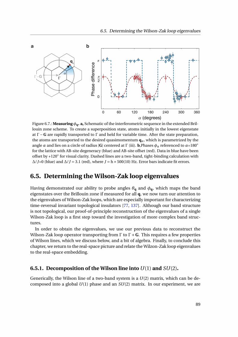
6.5. Determining the Wilson-Zak loop eigenvalues
0 60 120 180 240 300 360
0
2
Phas
e di
ffere
nce
(degrees)
a b
q
G
Figure 6.7.: Measuringφq. a, Schematic of the interferometric sequence in the extended Bril-louin zone scheme. To create a superposition state, atoms initially in the lowest eigenstateat Γ−G are rapidly transported to Γ and held for variable time. After the state preparation,the atoms are transported to the desired quasimomentum qα, which is parametrized by theangle α and lies on a circle of radius |G| centered at Γ (iii). b,Phases φα referenced to α=180
for the lattice with AB-site degeneracy (blue) and AB-site offset (red). Data in blue have beenoffset by +120 for visual clarity. Dashed lines are a two-band, tight-binding calculation with∆/J=0 (blue) and ∆/J = 3.1 (red), where J = h×500(10) Hz. Error bars indicate fit errors.
6.5. Determining the Wilson-Zak loop eigenvalues
Having demonstrated our ability to probe angles θq and φq, which maps the bandeigenstates over the Brillouin zone if measured for all q, we now turn our attention tothe eigenvalues of Wilson-Zak loops, which are especially important for characterizingtime-reversal invariant topological insulators [77, 137]. Although our band structureis not topological, our proof-of-principle reconstruction of the eigenvalues of a singleWilson-Zak loop is a first step toward the investigation of more complex band struc-tures.
In order to obtain the eigenvalues, we use our previous data to reconstruct theWilson-Zak loop operator transporting from Γ to Γ+G. This requires a few propertiesof Wilson lines, which we discuss below, and a bit of algebra. Finally, to conclude thischapter, we return to the real-space picture and relate the Wilzon-Zak loop eigenvaluesto the real-space embedding.
6.5.1. Decomposition of the Wilson line into U (1) and SU (2).
Generically, the Wilson line of a two-band system is a U (2) matrix, which can be de-composed into a global U (1) phase and an SU (2) matrix. In our experiment, we are
89
Chapter 6. Bloch state tomography with Wilson lines
able to measure only the SU (2) part. Indeed, the global phase does not show up onthe Bloch sphere, which represents a projected Hilbert space. That is, we obtain in-formation only about the rotations of a vector on the Bloch sphere, which is given bythe SU (2) part, while the entire Bloch sphere can be oriented in any way, which is theglobal gauge-freedom from the U (1) phase. Nonetheless, by examining the decompo-sition of the U (2) Wilson line, we can gain some insight into the quantities we are (andare not) measuring.
We begin by writing the Wilczek-Zee connection matrix Aq in a general form as
Aq =A1,1
q A1,2q
A2,1q A2,2
q
(6.23)
To simplify notation, we henceforth suppress the q subscript and note that all elementsare still to be understood as being q-dependent. Next, we decompose the matrix as
A =A1,1+A2,2
2 0
0 A1,1+A2,2
2
+A1,1−A2,2
2 A1,2
A2,1 −A1,1−A2,2
2
:= AU (1) + ASU (2) (6.24)
Noting that AU (1) is proportional to the identity matrix and therefore commutes withASU (2) and with itself for all quasimomenta, the Wilson line WQ→q transporting a statefrom initial quasimomentum Q to final quasimomentum q can be expressed as:
WQ→q =P e i∫C dqA
=P e i∫C dqAU (1)+ASU (2)
= e i∫C dqAU (1)P e i
∫C dqASU (2) (6.25)
where C denotes the path taken from Q to q. This completes the decomposition of theU (2) Wilson line into a U (1) global phase multiplied by a path-ordered SU (2) matrix.
Notably, the global U (1) phase is given by∫C
dqA1,1 +A2,2
2, (6.26)
which is simply the sum of the standard geometric phases acquired in the first andsecond band. That is, for a closed path, the U (1) phase is the sum of the Berry phasesand for a closed-by-a-reciprocal-lattice-vector path, the U (1) phase is sum of the Zakphases of the first and second band. Therefore, the U (1) phase encodes the first Chernnumber of the system [7, 90], which, for example, characterizes the celebrated integerquantum Hall effect [2, 144].
90
6.5. Determining the Wilson-Zak loop eigenvalues
For our purposes, we simply need to know that the experiment reconstructs an SU(2)matrix, which, in its most general form, can be written: W 11 W 12
−W 12∗ W 11∗
(6.27)
where∣∣W 11
∣∣2 + ∣∣W 12∣∣2 = 1. The eigenvalues e±iξ of this matrix are given by
Re[W 11]± i√∣∣W 12
∣∣2 + Im[W 11]2 (6.28)
Our measurements of θΓ+G give∣∣W 11
∣∣ and∣∣W 12
∣∣ = √1− ∣∣W 11
∣∣2. However, to find
the eigenvalues, we additionally need Arg[W 11] while our measurements of φΓ+G onlygive Arg[W 11]-Arg[W 12]. To find Arg[W 11], we will utilize a property of Wilson linescalled the back-tracking condition [145].
6.5.2. The back-tracking condition
For generic quasimomenta q and Q [145],
WQ→q = W†q→Q. (6.29)
Consequently, Wq→QWQ→q =1, such that going forward and back along the same pathresults in no transformation of the state vector. This is known as the back-trackingcondition.
In the case of the Wilson-Zak loop in the experiment, the relevant relation is
WΓ→Γ+G = W†Γ→Γ−G, (6.30)
where we have used that WΓ→Γ−G = WΓ+G→Γ which, assuming a periodic gauge choice,follows from the periodicity of the Brillouin zone. If the phase φΓ+G of the oscillationafter transport from Γ to Γ+G is given by
φΓ+G = Arg[W 11Γ→Γ+G]−Arg[W 12
Γ→Γ+G], (6.31)
then the phase φΓ−G of the oscillation after transport from Γ to Γ−G is
φΓ−G =−Arg[W 11Γ→Γ+G]−Arg[W 12
Γ→Γ+G]+π (6.32)
Therefore, taking the difference between the two oscillation phases extracts
91
Chapter 6. Bloch state tomography with Wilson lines
Arg[W 11Γ→Γ+G] as
φΓ+G −φΓ−G −π= 2Arg[W 11Γ→Γ+G] (6.33)
Note that there is an ambiguity in choosing±πwhen relatingφΓ+G toφΓ−G. This resultsin a global U (1) phase shift of π in the eigenvalue phases. However, the phase differ-ence between the eigenvalues is unaffected, which is sufficient to reconstruct, e.g., theZ2 invariant.
6.5.3. Wilson-Zak loop eigenvalues with and without inversionsymmetry
When the lattice is inversion symmetric, i.e., when A and B sites are degenerate, apply-ing Eq.6.33 to the phase of oscillations for α = 0 and α = 180 in the interferometricsequence (Fig. 6.7b) yields Arg[W 11
Γ→Γ+G]=0.03(7) rad. Combined with the direct trans-port data from Γ to Γ+G (Fig. 6.6b), which gives
∣∣W 11Γ→Γ+G
∣∣=0.47(2) and∣∣W 12
Γ→Γ+G
∣∣ =√1− ∣∣W 11
Γ→Γ+G
∣∣2=0.88(1), we obtain eigenvalue phases ξ = 1.03(2)π/3. These values
are in good agreement with the value of ξ=π/3 predicted from the two-band model.
In a lattice with AB-site offset, data for α = 0 and α = 180 from Fig. 6.7b yieldsArg[W 11
Γ→Γ+G]=-0.76(6) rad. We measure the absolute values by transporting atomsinitialized at Γ in the lowest eigenstate to Γ + G with increasing force. The re-maining population in the first band is shown in Fig. 6.8a. At |F|d/ε = 5, wherethe population transfer has saturated, we obtain
∣∣W 11Γ→Γ+G
∣∣=0.63(3) and∣∣W 12
Γ→Γ+G
∣∣ =√1− ∣∣W 11
Γ→Γ+G
∣∣2=0.77(2). This gives the eigenvalue phases of ξ = 1.04(4)π/3. Re-
markably, these eigenvalues are the same (within error bars) as the eigenvalues in aninversion-symmetric lattice.
Hence, while the data in, e.g., Fig. 6.7 measures different eigenstates, indicatingthat the (local) geometric structure of the bands have changed, the invariance of theWilson-Zak loop eigenvalues suggests that the (global) topological structure of thebands remains the same in lattices with and without inversion symmetry. This in-variance is a direct consequence of the real-space representation of the Wilson-Zakloop, WΓ→Γ+G = e i G·r. Since the Wilson-Zak loop depends only on the position oper-ator r, the eigenvalues are determined solely by the physical locations of the latticesites. Consequently, any perturbation, such as an energy offset between A and B sites,that does not invalidate the completeness assumption we used to formulate the path-independent Wilson line and does not change the position of the lattice sites will yieldthe same Wilson-Zak loop eigenvalues.
92
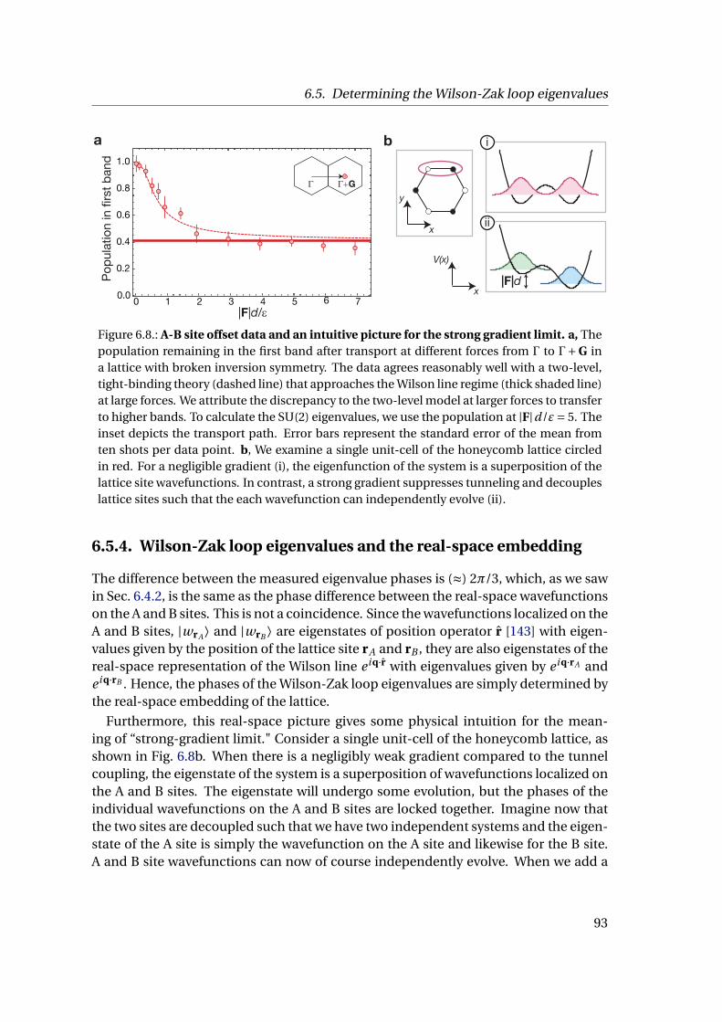
6.5. Determining the Wilson-Zak loop eigenvalues
0 1 2 3 4 5 6 70.0
0.2
0.4
0.6
0.8
1.0
|F|d/ε
Popu
latio
n in
firs
t ban
d
Γ Γ+G
a b
V(x)
x
y
x
|F|d
i
ii
Figure 6.8.: A-B site offset data and an intuitive picture for the strong gradient limit. a, Thepopulation remaining in the first band after transport at different forces from Γ to Γ+G ina lattice with broken inversion symmetry. The data agrees reasonably well with a two-level,tight-binding theory (dashed line) that approaches the Wilson line regime (thick shaded line)at large forces. We attribute the discrepancy to the two-level model at larger forces to transferto higher bands. To calculate the SU(2) eigenvalues, we use the population at |F|d/ε= 5. Theinset depicts the transport path. Error bars represent the standard error of the mean fromten shots per data point. b, We examine a single unit-cell of the honeycomb lattice circledin red. For a negligible gradient (i), the eigenfunction of the system is a superposition of thelattice site wavefunctions. In contrast, a strong gradient suppresses tunneling and decoupleslattice sites such that the each wavefunction can independently evolve (ii).
6.5.4. Wilson-Zak loop eigenvalues and the real-space embedding
The difference between the measured eigenvalue phases is (≈) 2π/3, which, as we sawin Sec. 6.4.2, is the same as the phase difference between the real-space wavefunctionson the A and B sites. This is not a coincidence. Since the wavefunctions localized on theA and B sites, |wrA⟩ and |wrB ⟩ are eigenstates of position operator r [143] with eigen-values given by the position of the lattice site rA and rB , they are also eigenstates of thereal-space representation of the Wilson line e i q·r with eigenvalues given by e i q·rA ande i q·rB . Hence, the phases of the Wilson-Zak loop eigenvalues are simply determined bythe real-space embedding of the lattice.
Furthermore, this real-space picture gives some physical intuition for the mean-ing of “strong-gradient limit." Consider a single unit-cell of the honeycomb lattice, asshown in Fig. 6.8b. When there is a negligibly weak gradient compared to the tunnelcoupling, the eigenstate of the system is a superposition of wavefunctions localized onthe A and B sites. The eigenstate will undergo some evolution, but the phases of theindividual wavefunctions on the A and B sites are locked together. Imagine now thatthe two sites are decoupled such that we have two independent systems and the eigen-state of the A site is simply the wavefunction on the A site and likewise for the B site.A and B site wavefunctions can now of course independently evolve. When we add a
93
Chapter 6. Bloch state tomography with Wilson lines
sufficiently strong gradient, we effectively decouple A and B sites by suppressing thetunneling, thereby enabling independent evolution of A and B site real-space wave-functions. Consequently, in this picture, entering the strong-gradient regime dependson whether the gradient over the distance between A and B sites, |F|d , is sufficientlylarger than the tunneling.
94
Chapter 7.
Conclusion and Outlook
Novel detection methods are essential in the study of band structure topology using ul-tracold atoms in optical lattices. Although classic transport measurements from con-densed matter physics [26] have been successfully used in ultracold atom setups [55–58], the ability to access new observables is a very compelling motivation for the devel-opment of techniques specific to cold atom systems [71, 146–157]. Notably, cold atomexperiments offer the unique opportunity to directly probe the band geometry [72, 136,137, 158]. In this thesis, we demonstrated two such detection methods using a BEC of87Rb in the s-bands of an optical honeycomb lattice.
Both methods can be understood by considering the general problem of a single-particle confined to a periodic potential and subjected to a constant, external force. Wederived the equations of motion for this problem in the basis of the band eigenstatesin Chapter 2 and discovered that the non-Abelian Berry connections are responsiblefor interband transitions. We then proceeded to analyze the two limiting cases of avery small and very large force, where very small and very large is defined relative tothe energy splitting between the bands. In the former scenario, interband transitionscan be neglected and atoms in each band independently acquire Berry phases, whilein the latter situation, the interband transitions dominate and the dispersion can beneglected. In this case, the unitary time evolution operator is no longer just a phasefactor, but a matrix-valued quantity termed the Wilson line. Our goal then, was tomeasure the Berry phase and the Wilson line in order to probe the geometric structureof the bands.
In the first set of experiments (Chapter 5), we realized an atomic interferometer tomeasure the π Berry flux associated with a Dirac cone in reciprocal space, in analogyto an Aharonov-Bohm interferometer that measures the magnetic flux penetrating agiven area in real space. Using a spin-echo sequence, we measured a Berry flux of0.95(10)π and constrained the spread in Berry curvature of a Dirac point to be smallerthan 10−3kL . Our results are consistent with a perfectly localized Berry curvature, in-dicating both the high resolution of our interferometer and the quality of our opticallattice. Furthermore, by imbalancing the lattice beams, we tracked the movement andeventual annihilation of the Dirac points.
In principle, by combining local measurements of the Berry flux in small interfer-
95
Chapter 7. Conclusion and Outlook
ometer loops, we could reconstruct the distribution of Berry curvature in the Brillouinzone and directly obtain the Chern number of the band. In practice, however, thismethod has a few disadvantages. First, the measurement crucially depends on the can-cellation of dynamical phases. This is accomplished by the spin-echo sequence whenthe symmetry axis of the interferometer loop coincides with the symmetry axis of thedispersion relation. However, for off-center loops, dynamical phases are not cancelled.Second, the spin-echo sequence requires a stable magnetic field, which, depending onthe level of stability, can be challenging to technically achieve. While neither issue isinsurmountable, it is prudent to consider whether there exists a simpler alternative.To this end, we examined a technique for Bloch state tomography using Wilson linesin Chapter 6.
By appropriately choosing the magnitude of the force, we realized strong-gradientdynamics that are described by the Wilson line operator and measured its elementsin the basis of the band eigenstates. We noted that, although Wilson lines are gener-ally path-ordered, they are in fact path-independent in the s-bands of the honeycomblattice, where the Hilbert subspace is the same at all quasimomenta. This simplifica-tion enabled us to relate the Wilson line elements to an overlap between cell-periodicBloch functions and thereby map the geometric structure of the bands over the en-tire Brillouin zone. We noted that even in more complex band structures where theHilbert space is quasimomentum-dependent, the same experimental techniques canbe used. To characterize such bands, we would reconstruct Wilson-Zak loops (in thebasis of the band eigenstates) and access the eigenvalues. As a proof-of-principle, wedemonstrated the reconstruction of a single Wilson-Zak loop in our standard honey-comb lattice. We showed that, although the band eigenstates change, the Wilson-Zakloop eigenvalues remain the same when inversion symmetry is broken, corroboratingthe fact that these eigenvalues identify the topological nature of the bands.
The Wilson line technique is a convenient and straight-forward way to character-ize band structures. It does not require a magnetic field, can be readily used to probethe entire Brillouin zone, and occurs at relatively fast time-scales which is advanta-geous for heating issues. However, a main limitation is the requirement of the strong-gradient condition. In other words, the technique is only applicable in band structuresthat contain a set of bands which are well-separated from other bands. This naturallyoccurs in lattices with multiple sites per unit cell, such as, for example, our familiarhoneycomb lattice, the Lieb lattice, or the Kagome lattice [159]. However, in alignmentwith the more general goal of band structure engineering, it may also be possible tocreate band structures that fulfill this condition.
7.1. Outlook
Equipped with our new detection techniques, the next goal is to engineer band struc-tures with the desired geometric or topological features. To this end, we have started
96

7.1. Outlook
a c
Ener
gy
Ener
gy
Ener
gy
Ener
gydetuning quasimomentum
rot. frame
rot. frame
b d quasimomentum quasimomentum
Figure 7.1.: An analogy between coupling a two-level atom and two energy bands. a, Twoenergy levels (red and green bars) of an atom are coupled by an electromagnetic field (bluearrow). Here, we show a field that is blue-detuned by δ from the atomic resonance. Right:Depiction of energy levels in a frame co-rotating with the electromagnetic field, where theground state (red) is shifted up in energy by the field frequency. b, Eigenenergies of the bareatomic Hamiltonian (solid lines) and coupled Hamiltonian (dashed lines) as function of de-tuning. c, Two energy bands (red and green) are coupled by a time-periodic modulation ofthe lattice (blue arrow). Here, we show a modulation frequency blue-detuned by δ from theΓ point. Since the energy bands are quasimomentum-dependent, the modulation becomesmore detuned at quasimomentum away from Γ. For clarity, the lowest two bands of a 1D lat-tice are depicted. However, the same picture applies to the more complex band structure of,e.g., a honeycomb lattice. Right: Energy bands in a frame co-rotating with the modulation.d, Energy bands of the static lattice (solid lines) and the modulated lattice (dashed lines) asfunction of quasimomentum. Note that the dashed red band exhibits two minima.
to investigate the effect of time-periodic modulations of the phase and intensity ofthe lattice beams. To form an intuition for how time-periodic modulations changesthe band structure, we draw an analogy to the problem of a two-level atom coupledby a semi-classical electromagnetic field, as depicted in Fig. 7.1a. By applying therotating-wave approximation and entering a frame co-rotating with the field, we ob-tain a time-dependent Hamiltonian parametrized only by the detuning and the cou-pling strength [160].
When there is no coupling, the eigenstates of this time-dependent Hamiltonian aresimply the bare atomic states and, at zero detuning, the eigenenergies are degener-ate (see Fig. 7.1b). When there is coupling, the new eigenstates, which are commonlycalled the dressed states, are superpositions of the bare atomic states. Furthermore,the degeneracy at zero detuning is broken . Hence, by coupling the ground and excited
97
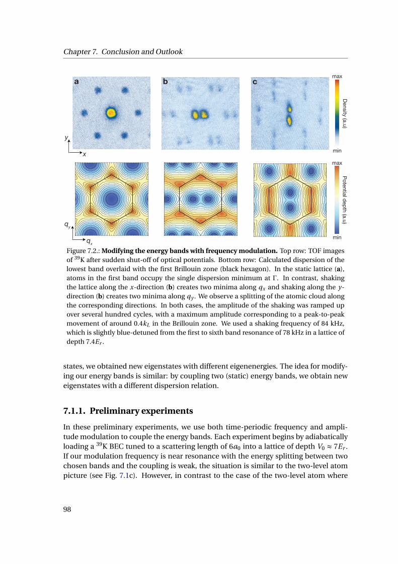
Chapter 7. Conclusion and Outlook
y
x
qy
qx
a b
Density (a.u)
min
max
Potential depth (a.u)
min
max
c
Figure 7.2.: Modifying the energy bands with frequency modulation. Top row: TOF imagesof 39K after sudden shut-off of optical potentials. Bottom row: Calculated dispersion of thelowest band overlaid with the first Brillouin zone (black hexagon). In the static lattice (a),atoms in the first band occupy the single dispersion minimum at Γ. In contrast, shakingthe lattice along the x-direction (b) creates two minima along qx and shaking along the y-direction (b) creates two minima along qy . We observe a splitting of the atomic cloud alongthe corresponding directions. In both cases, the amplitude of the shaking was ramped upover several hundred cycles, with a maximum amplitude corresponding to a peak-to-peakmovement of around 0.4kL in the Brillouin zone. We used a shaking frequency of 84 kHz,which is slightly blue-detuned from the first to sixth band resonance of 78 kHz in a lattice ofdepth 7.4Er .
states, we obtained new eigenstates with different eigenenergies. The idea for modify-ing our energy bands is similar: by coupling two (static) energy bands, we obtain neweigenstates with a different dispersion relation.
7.1.1. Preliminary experiments
In these preliminary experiments, we use both time-periodic frequency and ampli-tude modulation to couple the energy bands. Each experiment begins by adiabaticallyloading a 39K BEC tuned to a scattering length of 6a0 into a lattice of depth V0 ≈ 7Er .If our modulation frequency is near resonance with the energy splitting between twochosen bands and the coupling is weak, the situation is similar to the two-level atompicture (see Fig. 7.1c). However, in contrast to the case of the two-level atom where
98

7.1. Outlook
the detuning is a tunable attribute of the applied electromagnetic field, the detun-ing in the band structure is parametrized by the quasimomentum. That is, due to thequasimomentum-dependence of the energy bands, a given modulation frequency nat-urally results in a quasimomentum-dependent detuning. In Fig. 7.1d, we schematicallydepict coupling two bands with a frequency slightly blue of the energy gap atΓ to createa "dressed state" band with two minima. This has been already been experimentallyachieved in a 1D lattice [68].
In our first experiment, we modulate the frequency of the lattice beams at a fre-quency slightly blue-detuned of frequency gap between the first and the sixth bandat Γ. Similar to the 1D experiment [68], this creates a dispersion with two minima.After loading the BEC, we "shake" the lattice along one direction for roughly 10 ms,which corresponds to approximately 1000 modulation cycles. Here, "shaking" the lat-tice means that the entire lattice potential is moving back and forth1. Next, we abruptlyshut off all optical potentials and image the atoms after TOF. In contrast to TOF imagesfrom a static lattice, we see atoms occupy two distinct minima, which clearly indicatesa modified dispersion relation (see top row of Fig. 7.2). The direction along which thecloud splits depends on the direction of the shaking and is in good (qualitative) agree-ment with theory (bottom row of Fig. 7.2).
In addition to the modified dispersion relation, a second signature of coupling be-tween bands is the presence of Rabi oscillations. Similar to the two-level atom, wherethe population oscillates between the ground and the excited state, we expect the pop-ulation to oscillate between the ground band and the coupled band. Indeed, we ob-serve oscillations between bands when modulating either the frequency or the am-plitude of the lattice beams. We show a typical Rabi oscillation in Fig. 7.3, where theamplitude of a single beam was modulated resonant to the energy gap between thefirst and third band at Γ. In order to selectively transfer atoms into only the third band,we imbalanced the power of one beam relative to the other two. This breaks the C3
symmetry of the lattice and lifts the degeneracy between the third and fourth bands atΓ. We confirmed that the atoms populated primarily the third band by band mapping.
Beyond qualitative observations, the two-level atom analogy also helps in derivingan expression for the Rabi frequency of our system. This allows us to make quantita-tive comparisons between theory and experiment. We begin by Taylor expanding theHamiltonian in the time-periodic perturbation. That is, if the original Hamiltonian isH(V ), then our modulated Hamiltonian is H(V +εcos(ωt )), where V +εcos(ωt ) repre-sents the potential with a periodic modulation, ω is the frequency of the modulationand ε gives the amplitude of the modulation. Here, we have made no assumption onthe type of modulation—εcos(ωt ) can refer to either frequency2 or amplitude modu-
1 Recall from Sec. 4.3.2 that changing the frequency of a given lattice beam shifts the entire potentialalong the propagation direction of that beam. Accordingly, sinusoidal modulation of the frequencyof a lattice beam "shakes" the potential back and forth.
2 In the specific case of frequency modulation, this formalism can be connected to the equations ofmotion we derived in Sec. 2.2.2. There, we saw that the coupling between bands was given by the
99
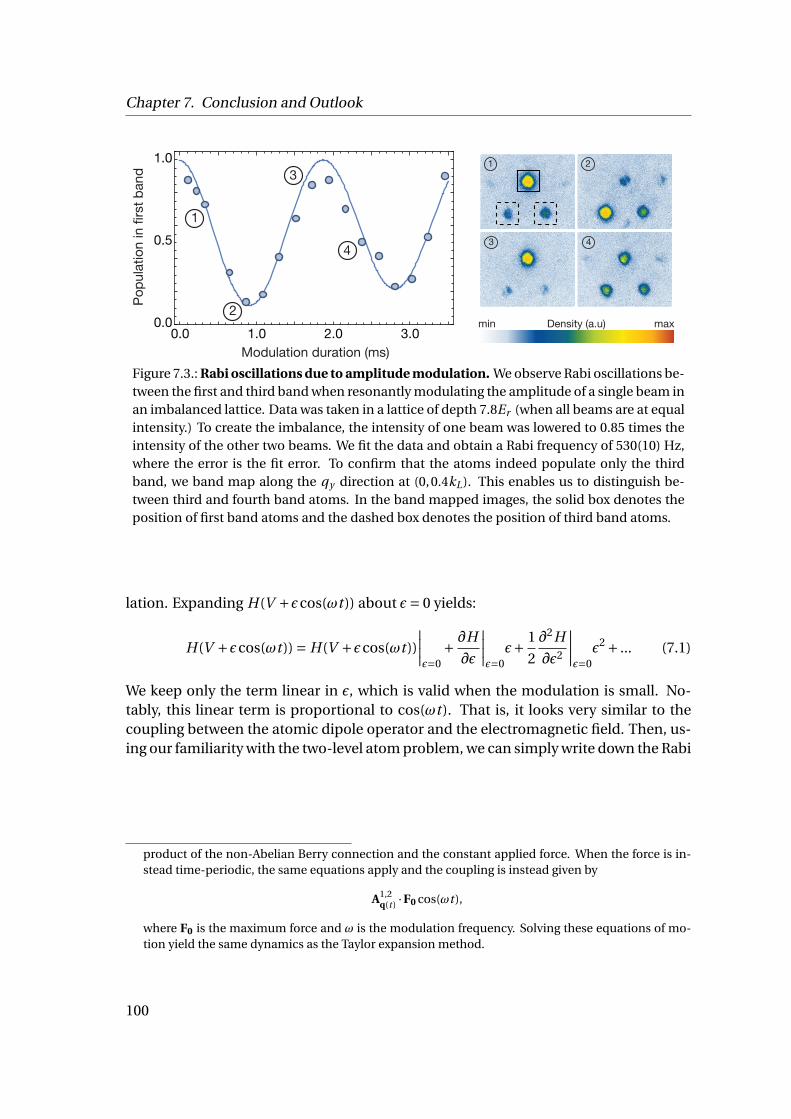
Chapter 7. Conclusion and Outlook
0.0 1.0 2.0 3.00.0
0.5
1.0Po
pula
tion
in fi
rst b
and
Modulation duration (ms)
Density (a.u)min max
1
2
3
4
1 2
3 4
Figure 7.3.: Rabi oscillations due to amplitude modulation. We observe Rabi oscillations be-tween the first and third band when resonantly modulating the amplitude of a single beam inan imbalanced lattice. Data was taken in a lattice of depth 7.8Er (when all beams are at equalintensity.) To create the imbalance, the intensity of one beam was lowered to 0.85 times theintensity of the other two beams. We fit the data and obtain a Rabi frequency of 530(10) Hz,where the error is the fit error. To confirm that the atoms indeed populate only the thirdband, we band map along the qy direction at (0,0.4kL). This enables us to distinguish be-tween third and fourth band atoms. In the band mapped images, the solid box denotes theposition of first band atoms and the dashed box denotes the position of third band atoms.
lation. Expanding H(V +εcos(ωt )) about ε= 0 yields:
H(V +εcos(ωt )) = H(V +εcos(ωt ))
∣∣∣∣ε=0
+ ∂H
∂ε
∣∣∣∣ε=0
ε+ 1
2
∂2H
∂ε2
∣∣∣∣ε=0
ε2 + ... (7.1)
We keep only the term linear in ε, which is valid when the modulation is small. No-tably, this linear term is proportional to cos(ωt ). That is, it looks very similar to thecoupling between the atomic dipole operator and the electromagnetic field. Then, us-ing our familiarity with the two-level atom problem, we can simply write down the Rabi
product of the non-Abelian Berry connection and the constant applied force. When the force is in-stead time-periodic, the same equations apply and the coupling is instead given by
A1,2q(t ) ·F0 cos(ωt ),
where F0 is the maximum force and ω is the modulation frequency. Solving these equations of mo-tion yield the same dynamics as the Taylor expansion method.
100
7.1. Outlook
frequencyΩ coupling the two bands as 3
Ω= ε
cos(ωt )
∂H
∂ε
∣∣∣∣ε=0
. (7.3)
Remarkably, this simple calculation yields Rabi frequencies that are well-matchedby experiment. For example, the data in Fig. 7.3 yields a Rabi frequency of 530(10) Hz,which is well within the predicted range of 465 Hz to 775 Hz for a modulation depth of2.0(5)%.4
7.1.2. Next steps
Our preliminary experiments demonstrate coherent coupling between bands of thehoneycomb lattice. As a next step, we would like to more thoroughly follow-up onthese encouraging results. For example, it would be interesting to examine how thesymmetry of the modulation influences which bands can be coupled. In a monoatomiclattice, the parity of the Bloch states determines which bands can be coupled with fre-quency or amplitude modulation [161]. Understanding the corresponding "selectionrules" in the honeycomb lattice, which has two sites per unit cell, informs us whetherto use phase or amplitude modulation or perhaps a combination of both to couple tothe desired band.
This coherent control could subsequently be used to observe quantum optics phe-nomena, such as electromagnetically-induced transparency [162], in the bands of anoptical lattice. Furthermore, coherent transfer of atoms into a higher band with nearlyunit efficiency allows for the exploration of orbital physics [163]. Moreover, we couldinvestigate flat band physics [94, 164, 165] by transferring atoms into the p-bands ofthe honeycomb lattice, which contain flat bands [166, 167], and adding interactionsvia Feshbach resonances. These directions all require first examining the lifetime ofthe atoms in the higher bands.
More closely related to the contents of this thesis, coherent coupling between bandsmay also offer a promising way to realize path-dependent and possible non-abelianWilson lines. The experiments in this thesis took place entirely within the s-bands
3 Explicitly: Let the potential and perturbation be f =V +εcosωt . Then,
∂H
∂ε
∣∣∣∣ε=0
ε= ∂H
∂ f
∂ f
∂ε
∣∣∣∣ε=0
ε= ∂H
∂ f
∣∣∣∣ε=0
εcosωt . (7.2)
This looks very similar to the coupling d ·Ecosω′t between the dipole moment of an atom d and theelectric field Ecosω′t , where E gives the amplitude and polarization of the electric field and ω′ is itsfrequency.
4 At the time the data was taken, our primary experimental uncertainty was the modulation depth be-cause of some technical issues. After resolving these problems, a more recent measurement yieldeda Rabi frequency of 616(6) Hz compared to the predicted value of 619 Hz.
101
Chapter 7. Conclusion and Outlook
of the honeycomb lattice, where the Hilbert subspace is the same at every quasimo-mentum, and, as a consequence, the Wilson lines are path-independent. To createa quasimomentum-dependent Hilbert subspace, we could couple an s-band to a p-band. This introduces a quasimomentum-dependent admixture of p-band characterinto the two lowest bands of the honeycomb lattice.
In addition to schemes that rely on coupling to higher orbital bands, we are also cur-rently investigating the possibility of realizing path-dependent Wilson lines by intro-ducing a spin degree of freedom. These experiments would require a spin-dependentlattice and coupling between both the s-bands and the spin states. The main challengein either case of using spin states or higher orbital bands is to ensure that the strong-gradient condition can still be fulfilled in the modified band structure.
In a broader context, our investigations into time-periodic modulations of the lat-tice are ultimately directed toward engineering the band geometry. While our two levelanalogy provides some intuition on how the dispersion of the bands are modified, Flo-quet theory is required for a full analysis. Floquet theory encompasses our simple two-level picture and is a general framework where a time-periodic Hamiltonian is mappedonto an effective time-independent Hamiltonian, commonly called the Floquet Hamil-tonian [65, 168]. It has recently been shown, both theoretically and experimentally,that Floquet Hamiltonians can have different topological properties from the original,static Hamiltonian [67, 168]. For example, in ultracold atom systems, Floquet theoryunderlies the recent work on the Haldane model [55] and the experiments realizingstrong artificial magnetic fields in optical lattices [56, 62, 63, 169, 170]. Therefore, rein-terpreted in terms of Floquet theory, our investigations into the details of amplitudeand frequency modulation are directly relevant for engineering the geometry of bandstructures.
7.1.3. Future endeavors
Beyond our more immediate goals, which can all be described within a single-particleframework, lies the exciting prospect of exploring phenomena that arise from the in-terplay between topology and strong interactions. One such example is the paradig-matic fractional quantum Hall effect [171–173], where elementary excitations canhost fractional charges and obey anyonic statistics, which are neither bosonic norfermionic [174, 175]. An experimental observation of non-abelian anyonic statisticswould be a breakthrough step toward topological quantum computing [176]. Further-more, while the fractional quantum Hall effect, like its integer counterpart, occurs atstrong magnetic fields and low temperatures, similar states, called fractional Chern in-sulators, are predicted to exist at zero magnetic field and room temperatures [177, 178];they have, however, not yet been experimentally realized. Finally, another intriguingdirection could be the investigation of topological Mott insulators, where interactionsinduce the transition into a topological phase [9, 179].
In all of these endeavors, control over the interactions between particles is central.
102
7.1. Outlook
This requirement is fulfilled in our ultracold atom systems by Feshbach resonances,which can be used to continuously tune interactions over a wide range [38]. In concertwith Floquet theory, this gives us the necessary tools with which to engineer topologi-cal systems with strong interactions. However, one primary challenge is to understandthe heating rates in periodically-modulated lattice systems. Indeed, in our preliminaryexperiments with amplitude and phase modulation, we used 39K atoms tuned to a lowscattering length for precisely this reason. Initial tries with 87Rb, which does not havean easily accessible Feshbach resonance, resulted in significant heating in the modu-lated lattice.
At present, the modulation-induced heating seen in experiments [62, 180] is poorlyunderstood. However, in recent years, there have been an increasing number of theo-retical investigations into the topic [181–189]. In parallel, experiments [190], includingours, have begun systematic studies into heating rates with various lattice and modu-lation parameters. A better understanding of the interaction effects in driven systemsand the identification of optimal modulation regimes are essential to the ultimate goalof exploring strongly-interacting topological systems with ultracold atom systems.
103

Appendix A.
Experimental details
We begin this section by describing details of the vacuum setup, coil configuration,and laser system. In particular, we explain the reasoning behind several main designdecisions and note the vendors from which we purchased key components.
Next, we outline our experimental sequence. Creating BECs is, by now, quite stan-dard fare. Rather than review the mechanisms of each step here, we instead commenton the specifics of our sequence. Reviews on the preparation of BECs can be found inRefs. [111, 191, 192]. Technical details can be found in Refs. [161, 193–195]. A compre-hensive overview of our setup can be also found in Ref. [78], which additionally dis-cusses the preparation of degenerate Fermi gases of 40K in our setup. Refs. [196, 197]discuss the construction and characterization of our 2D+-MOT and Ref. [198] detailsthe set-up of the laser system for our dipole trap.
A.1. The vacuum setup
The vacuum system consists of three chambers (see Fig. A.1a): the 2D+-MOT, the 3D-MOT, and the experiment cell. Each of these chambers is connected by a differentialpumping section, which enables a gradient of progressively lower pressure from the2D+-MOT to the experiment cell. A low pressure is desirable in the science cell to limitheating due to collisions with background atoms.
In the 2D+-MOT, which is connected to our sources of rubidium (Rb) and potassium(K), the pressure is 5 ×10⁻⁵ mbar. Our source of Rb was purchased from Alfa Aesar andcontains its two naturally occurring bosonic isotopes, 85Rb and 87Rb, in a respectiverelative abundance of 72.2% and 27.8% [99]. Our source of K was purchased from TraceSciences and is enriched to contain 3% of fermionic 40K, 9% of bosonic 41K, and 88%of bosonic 39K. These sources are contained in heated bellows which are connected tothe main 2D+-MOT chamber via a six-way cross, as shown in Fig. A.1b. The valves wereopened during the initial setup of the apparatus several years ago but are currentlyclosed.
The 2D+-MOT and its optics were built on a separate breadboard and are connectedto the 3D-MOT by a valve and a flexible bellow. The idea was to be able to slightly shiftthe entire 2D+-MOT apparatus relative to the 3D-MOT, in case the push beam of the
105
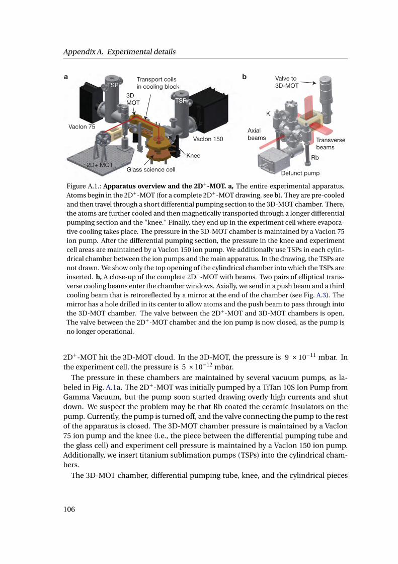
Appendix A. Experimental details
VacIon 75
2D+ MOTGlass science cell
3D MOT
a bTransport coils in cooling block
VacIon 150
TSP
TSP
Rb
K
Defunct pump
Transverse beams
Axial beams
Valve to 3D-MOT
Knee
Figure A.1.: Apparatus overview and the 2D+-MOT. a, The entire experimental apparatus.Atoms begin in the 2D+-MOT (for a complete 2D+-MOT drawing, see b). They are pre-cooledand then travel through a short differential pumping section to the 3D-MOT chamber. There,the atoms are further cooled and then magnetically transported through a longer differentialpumping section and the "knee." Finally, they end up in the experiment cell where evapora-tive cooling takes place. The pressure in the 3D-MOT chamber is maintained by a VacIon 75ion pump. After the differential pumping section, the pressure in the knee and experimentcell areas are maintained by a VacIon 150 ion pump. We additionally use TSPs in each cylin-drical chamber between the ion pumps and the main apparatus. In the drawing, the TSPs arenot drawn. We show only the top opening of the cylindrical chamber into which the TSPs areinserted. b, A close-up of the complete 2D+-MOT with beams. Two pairs of elliptical trans-verse cooling beams enter the chamber windows. Axially, we send in a push beam and a thirdcooling beam that is retroreflected by a mirror at the end of the chamber (see Fig. A.3). Themirror has a hole drilled in its center to allow atoms and the push beam to pass through intothe 3D-MOT chamber. The valve between the 2D+-MOT and 3D-MOT chambers is open.The valve between the 2D+-MOT chamber and the ion pump is now closed, as the pump isno longer operational.
2D+-MOT hit the 3D-MOT cloud. In the 3D-MOT, the pressure is 9 ×10⁻¹¹ mbar. Inthe experiment cell, the pressure is 5 ×10⁻¹² mbar.
The pressure in these chambers are maintained by several vacuum pumps, as la-beled in Fig. A.1a. The 2D+-MOT was initially pumped by a TiTan 10S Ion Pump fromGamma Vacuum, but the pump soon started drawing overly high currents and shutdown. We suspect the problem may be that Rb coated the ceramic insulators on thepump. Currently, the pump is turned off, and the valve connecting the pump to the restof the apparatus is closed. The 3D-MOT chamber pressure is maintained by a VacIon75 ion pump and the knee (i.e., the piece between the differential pumping tube andthe glass cell) and experiment cell pressure is maintained by a VacIon 150 ion pump.Additionally, we insert titanium sublimation pumps (TSPs) into the cylindrical cham-bers.
The 3D-MOT chamber, differential pumping tube, knee, and the cylindrical pieces
106
A.1. The vacuum setup
housing the titanium sublimation pumps were self-designed and machined out of(non-magnetic) stainless steel by Pink GmbH Vakuumtechnik.
The main chamber of the 2D+-MOT was self-designed and machined from titaniumby Vaqtec-scientific. Since the windows are directly glued onto the body of the cham-ber in our 2D+-MOT design, one concern was that vacuum leaks would be introduceddue to material deformation when heating the apparatus. To minimize this risk, wechose titanium for the body of the chamber and BK7 glass for the windows becausetitanium and BK7 have similar thermal expansion coefficients.
Other vacuum components, such as bellows, valves, and flanges, were purchasedfrom VAT Vakuumventile AG or VACOM. Flanged windows for, e.g, the 3D-MOT, werepurchased from Kurt J. Lesker.
Pictures of the actual experimental apparatus are shown in Fig. A.3.
A.1.1. The magnetic transport coils and the experiment cell
We self-wound the 2D+-MOT coils, the push coil, the experiment coils, and the biascoils around the 3D-MOT and the experiment cell. As its name suggests, the 2D+-MOTcoils provide the field gradient for the 2D+-MOT. These coils were soaked in thermallyconductive Electrolube ER2183 resin. The push coil is part of the magnetic transport,and the experiment coils provide the fields for the experiment cell. Each set of biascoils consist of a pair of coils along the x-, y-, and z-directions to offset, i.e., bias, theearth’s magnetic field and other constant fields in the lab (from assorted metal pieces,furniture, etc.). All other coils were wound by Oswald Elektromotoren GmbH.
The main magnetic transport setup consists of a push coil, one pair of 3D-MOT coils,15 pairs of transport coils, and one pair of experiment coils, as illustrated in Fig. A.2.The push coil is used to push the low-field seeking atoms toward the transport coils andcontrol the aspect ratio of the atomic cloud [112, 121, 196]. This is necessary becauseof the relatively large distance between the centers of the 3D-MOT coils and the first setof transport coils, which results in a weak gradient along the transport direction and anelongated atomic cloud
The 3D-MOT coils and all transport coils were glued into a self-designed coil hous-ing by Oswald Elektromotoren GmbH using Stycast FT 2850 and resined with AralditeF, which are both thermally conductive. Since we directly cool only the housing by run-ning water through it, good thermal conductivity between the housing and the coils iscrucial to keep the coils cool during experimental runs. The water flowing into thehousing is temperature stabilized at 20C by a Kühlmobil van der Heijden chiller. Thehousing was machined out of brass by the MPQ workshop.
The experiment coils
The design of the experiment coils required extra attention. There were certain re-quirements we wanted to meet: we desired a high gradient of around 300 G/cm for
107
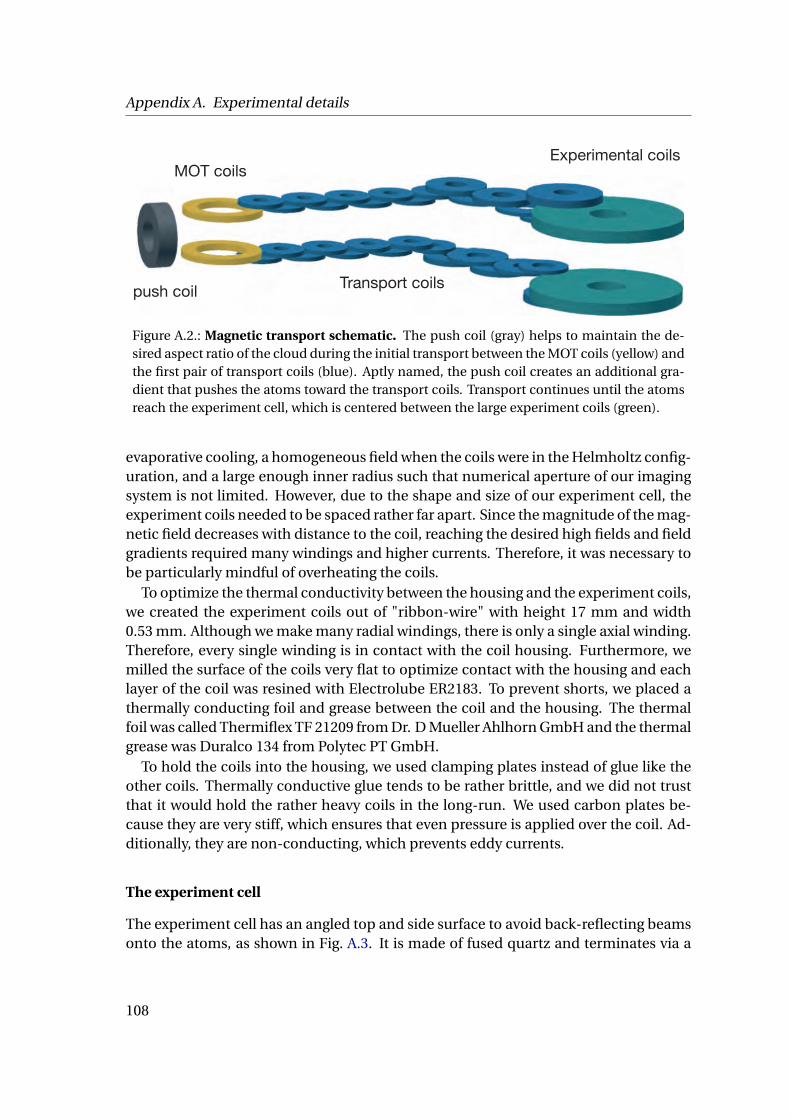
Appendix A. Experimental details
Push coil
MOT coilsTransport coils
Experiment coils
push coil
MOT coils
Transport coils
Experimental coils
Figure A.2.: Magnetic transport schematic. The push coil (gray) helps to maintain the de-sired aspect ratio of the cloud during the initial transport between the MOT coils (yellow) andthe first pair of transport coils (blue). Aptly named, the push coil creates an additional gra-dient that pushes the atoms toward the transport coils. Transport continues until the atomsreach the experiment cell, which is centered between the large experiment coils (green).
evaporative cooling, a homogeneous field when the coils were in the Helmholtz config-uration, and a large enough inner radius such that numerical aperture of our imagingsystem is not limited. However, due to the shape and size of our experiment cell, theexperiment coils needed to be spaced rather far apart. Since the magnitude of the mag-netic field decreases with distance to the coil, reaching the desired high fields and fieldgradients required many windings and higher currents. Therefore, it was necessary tobe particularly mindful of overheating the coils.
To optimize the thermal conductivity between the housing and the experiment coils,we created the experiment coils out of "ribbon-wire" with height 17 mm and width0.53 mm. Although we make many radial windings, there is only a single axial winding.Therefore, every single winding is in contact with the coil housing. Furthermore, wemilled the surface of the coils very flat to optimize contact with the housing and eachlayer of the coil was resined with Electrolube ER2183. To prevent shorts, we placed athermally conducting foil and grease between the coil and the housing. The thermalfoil was called Thermiflex TF 21209 from Dr. D Mueller Ahlhorn GmbH and the thermalgrease was Duralco 134 from Polytec PT GmbH.
To hold the coils into the housing, we used clamping plates instead of glue like theother coils. Thermally conductive glue tends to be rather brittle, and we did not trustthat it would hold the rather heavy coils in the long-run. We used carbon plates be-cause they are very stiff, which ensures that even pressure is applied over the coil. Ad-ditionally, they are non-conducting, which prevents eddy currents.
The experiment cell
The experiment cell has an angled top and side surface to avoid back-reflecting beamsonto the atoms, as shown in Fig. A.3. It is made of fused quartz and terminates via a
108
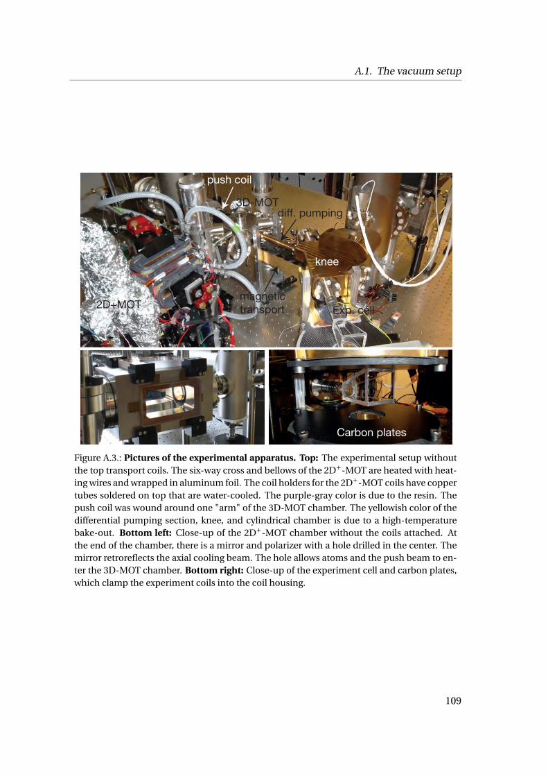
A.1. The vacuum setup
2D+MOT
3D-MOT
knee
push coil
magnetictransport
diff. pumping
Exp. cell
Carbon plates
Figure A.3.: Pictures of the experimental apparatus. Top: The experimental setup withoutthe top transport coils. The six-way cross and bellows of the 2D+-MOT are heated with heat-ing wires and wrapped in aluminum foil. The coil holders for the 2D+-MOT coils have coppertubes soldered on top that are water-cooled. The purple-gray color is due to the resin. Thepush coil was wound around one "arm" of the 3D-MOT chamber. The yellowish color of thedifferential pumping section, knee, and cylindrical chamber is due to a high-temperaturebake-out. Bottom left: Close-up of the 2D+-MOT chamber without the coils attached. Atthe end of the chamber, there is a mirror and polarizer with a hole drilled in the center. Themirror retroreflects the axial cooling beam. The hole allows atoms and the push beam to en-ter the 3D-MOT chamber. Bottom right: Close-up of the experiment cell and carbon plates,which clamp the experiment coils into the coil housing.
109

Appendix A. Experimental details
glass-to-metal seal in a metal flange that can be directly connected to the knee. Thecell was self-designed and constructed by Hellma Analytics.
A.2. The laser setup
A.2.1. Cooling in the 2D+-MOT and 3D-MOT
We use a total of 11 lasers to cool 87Rb and 39K in the 2D+-MOT and the 3D-MOT. Forcooling 87Rb, we have one reference laser, two repump lasers (one for each MOT), andtwo cooling lasers (one for each MOT). The reference and repump lasers are Toptica DLPros centered at 780 nm and have about 50 mW of output power. The cooling lasersare Toptica TA Pros (also centered at 780 nm) and have about 1 W of output power.
The hyperfine levels of the D2 line for 87Rb are shown in Fig. A.4 and labeled with therelevant transitions. The reference laser is so-called because it is the laser to which thefrequency of all the other lasers are referenced. To stabilize the frequency of the refer-ence laser, we use Doppler-free absorption spectroscopy and a frequency-modulationlock. All other lasers are locked using a delay-line lock which stabilizes the frequencydifference between a laser and the reference laser. In addition to being a frequency ref-erence, the reference laser is also used to spin polarize the atoms into |F = 2,mF = 2⟩state for magnetic transport and to image the atoms in the experiment cell.
The lasers used to cool 39K are very similar. We have one reference laser, two repumplasers, two cooling lasers, and one imaging laser. The reference and imaging lasers areToptica DL Pros and the cooling and repump lasers are Toptica TA Pros. These lasersare centered at 767 nm. The reason for using tapered-amplifier (TA) lasers with greaterpower for the repump light can be understood by considering the hyperfine splittingsfor 39K, as shown in Fig. A.4. Compared to the hyperfine splittings of 87Rb, those of 39Kare around an order of magnitude smaller. In fact, the detuning of both the repumpand cooling laser is roughly on the same order of magnitude as the hyperfine splitting.Consequently, the assumption of a cycling transition on the cooling line is not quitevalid; compared with the cooling transition of 87Rb, more atoms are being pumpedinto the |42S1/2,F = 1⟩ state and a greater repump intensity is required.
The light from the reference K laser is used only for locking purposes. The light fromthe imaging K laser is primarily used for imaging the atoms in the experiment cell, buta few mW is also used to spin polarize the atoms for magnetic transport.
All the lasers for the 2D+-MOT and 3D-MOT are on a separate optical table from theexperimental apparatus. The light is sent to the experiment via single-mode, polariza-tion maintaining fibers made by Nufern and sold by Thorlabs.
110
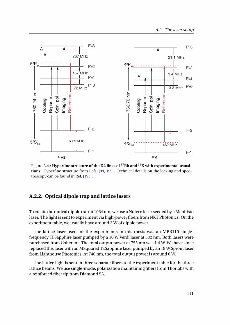
A.2. The laser setup
F'=0
F'=1
F'=2
F'=3
F=1
6835 MHz
F=2
∆
87Rb
52S1/2
52P3/2
F'=0
F'=1
F'=2
F'=3
F=1
21.1 MHz
462 MHz
9.4 MHz
3.3 MHz
F=276
6.70
nm
39K
42S1/2
42P3/2
Coo
ling
Repu
mp
Imag
ing
Refe
renc
e
Spin
pol
72 MHz
Coo
ling
Repu
mp
Imag
ing
Refe
renc
e
Spin
pol
157 MHz
267 MHz
780.
24 n
m
Figure A.4.: Hyperfine structure of the D2 lines of 87Rb and 39K with experimental transi-tions. Hyperfine structure from Refs. [99, 199]. Technical details on the locking and spec-troscopy can be found in Ref. [193].
A.2.2. Optical dipole trap and lattice lasers
To create the optical dipole trap at 1064 nm, we use a Nufern laser seeded by a Mephistolaser. The light is sent to experiment via high-power fibers from NKT Photonics. On theexperiment table, we usually have around 2 W of dipole power.
The lattice laser used for the experiments in this thesis was an MBR110 single-frequency Ti:Sapphire laser pumped by a 10 W Verdi laser at 532 nm. Both lasers werepurchased from Coherent. The total output power at 755 nm was 1.4 W. We have sincereplaced this laser with an MSquared Ti:Sapphire laser pumped by an 18 W Sprout laserfrom Lighthouse Photonics. At 740 nm, the total output power is around 6 W.
The lattice light is sent in three separate fibers to the experiment table for the threelattice beams. We use single-mode, polarization maintaining fibers from Thorlabs witha reinforced fiber tip from Diamond SA.
111
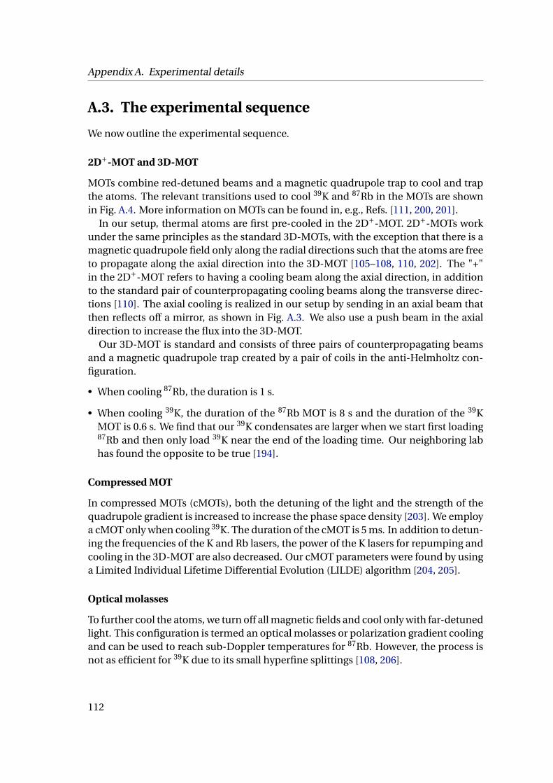
Appendix A. Experimental details
A.3. The experimental sequence
We now outline the experimental sequence.
2D+-MOT and 3D-MOT
MOTs combine red-detuned beams and a magnetic quadrupole trap to cool and trapthe atoms. The relevant transitions used to cool 39K and 87Rb in the MOTs are shownin Fig. A.4. More information on MOTs can be found in, e.g., Refs. [111, 200, 201].
In our setup, thermal atoms are first pre-cooled in the 2D+-MOT. 2D+-MOTs workunder the same principles as the standard 3D-MOTs, with the exception that there is amagnetic quadrupole field only along the radial directions such that the atoms are freeto propagate along the axial direction into the 3D-MOT [105–108, 110, 202]. The "+"in the 2D+-MOT refers to having a cooling beam along the axial direction, in additionto the standard pair of counterpropagating cooling beams along the transverse direc-tions [110]. The axial cooling is realized in our setup by sending in an axial beam thatthen reflects off a mirror, as shown in Fig. A.3. We also use a push beam in the axialdirection to increase the flux into the 3D-MOT.
Our 3D-MOT is standard and consists of three pairs of counterpropagating beamsand a magnetic quadrupole trap created by a pair of coils in the anti-Helmholtz con-figuration.
• When cooling 87Rb, the duration is 1 s.
• When cooling 39K, the duration of the 87Rb MOT is 8 s and the duration of the 39KMOT is 0.6 s. We find that our 39K condensates are larger when we start first loading87Rb and then only load 39K near the end of the loading time. Our neighboring labhas found the opposite to be true [194].
Compressed MOT
In compressed MOTs (cMOTs), both the detuning of the light and the strength of thequadrupole gradient is increased to increase the phase space density [203]. We employa cMOT only when cooling 39K. The duration of the cMOT is 5 ms. In addition to detun-ing the frequencies of the K and Rb lasers, the power of the K lasers for repumping andcooling in the 3D-MOT are also decreased. Our cMOT parameters were found by usinga Limited Individual Lifetime Differential Evolution (LILDE) algorithm [204, 205].
Optical molasses
To further cool the atoms, we turn off all magnetic fields and cool only with far-detunedlight. This configuration is termed an optical molasses or polarization gradient coolingand can be used to reach sub-Doppler temperatures for 87Rb. However, the process isnot as efficient for 39K due to its small hyperfine splittings [108, 206].
112
A.3. The experimental sequence
• When cooling 87Rb, the duration is 3 ms. We increase the detuning (more red) anddecrease the power of the Rb 3D-MOT cooling laser.
• When cooling 39K, the duration is 4.2 ms. We increase the detuning (more red) anddecrease the power of the Rb 3D-MOT cooling laser, the K 3D-MOT cooling laser,and the K 3D-MOT repumping laser. We found it particularly crucial to decrease thepower of the K 3D-MOT cooling laser.
Spin polarization
In this step, we pump the atoms into their |F = 2,mF = 2⟩ state in preparation for trans-port. Since only low-field seeking atoms are magnetically trappable, omitting this stepwould result in the loss of many atoms during magnetic transport. This procedure isalso called optical pumping.
The basic idea is to use a small offset field along, in our case, the z-axis to definea quantization axis and lift the degeneracy between magnetic sublevels. We then ap-ply σ+-polarized light resonant on the F = 2 to F ′ = 2 transition to induce transitionsthat increase the magnetic sublevel number. We also use σ+-polarized repump lightaddress atoms that decay into the F = 1 manifold. This optical pumping is quite effi-cient for both 87Rb and 39K. We end up with around 70% to 80% of both species in the|F = 2,mF = 2⟩ state.
These parameters were optimized using LILDE.
• For only 87Rb, the optical pumping duration is 0.7 ms.
• For 39K, the optical pumping duration is 0.8 ms for 87Rb and 0.5 ms for 39K.
Magnetic transport
After the spin polarization, we suddenly switch on a magnetic quadrupole field in the3D-MOT to a gradient strength of 45 G/cm to trap the atoms. As an additional pre-caution to transport primarily |F = 2,mF = 2⟩ atoms, we then ramp down the field in150 ms and hold at a lowered gradient of 28 G/cm for 200 ms. Holding at this loweredgradient ensures that 87Rb atoms in |F = 2,mF = 1⟩ leave the trap, since trapping 87Rbatoms in |F = 2,mF = 1⟩ requires a gradient strength of at least 30 G/cm, while trapping87Rb atoms in |F = 2,mF = 2⟩ requires only half that strength. (The gradients requiredfor 39K scale with the mass and require 13 G/cm and 6.5 G/cm. We cannot use thisramp down to remove |F = 2,mF = 2⟩ 39K atoms.)
Next, we ramp up the quadrupole field in 200 ms to the transport gradient of100 G/cm and move the atoms over a distance of 58 cm into the experiment cell [112,121, 196]. We lose about 80% of 87Rb atoms and 95% of 39K atoms once we hit the dif-ferential pumping section. This is due to both the small size of the differential pump-ing hole and an imperfect alignment of the transport coils relative to the center of the
113
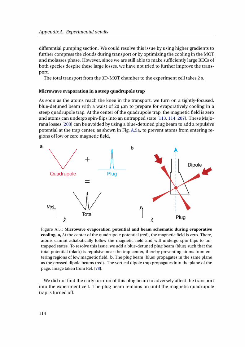
Appendix A. Experimental details
differential pumping section. We could resolve this issue by using higher gradients tofurther compress the clouds during transport or by optimizing the cooling in the MOTand molasses phase. However, since we are still able to make sufficiently large BECs ofboth species despite these large losses, we have not tried to further improve the trans-port.
The total transport from the 3D-MOT chamber to the experiment cell takes 2 s.
Microwave evaporation in a steep quadrupole trap
As soon as the atoms reach the knee in the transport, we turn on a tightly-focused,blue-detuned beam with a waist of 20 µm to prepare for evaporatively cooling in asteep quadrupole trap. At the center of the quadrupole trap, the magnetic field is zeroand atoms can undergo spin-flips into an untrapped state [113, 114, 207]. These Majo-rana losses [208] can be avoided by using a blue-detuned plug beam to add a repulsivepotential at the trap center, as shown in Fig. A.5a, to prevent atoms from entering re-gions of low or zero magnetic field.
ba
x
y
Plug
+
=
x
V(x)
DipoleQuadrupole Plug
Total
Figure A.5.: Microwave evaporation potential and beam schematic during evaporativecooling. a, At the center of the quadrupole potential (red), the magnetic field is zero. There,atoms cannot adiabatically follow the magnetic field and will undergo spin-flips to un-trapped states. To resolve this issue, we add a blue-detuned plug beam (blue) such that thetotal potential (black) is repulsive near the trap center, thereby preventing atoms from en-tering regions of low magnetic field. b, The plug beam (blue) propagates in the same planeas the crossed dipole beams (red). The vertical dipole trap propagates into the plane of thepage. Image taken from Ref. [78].
We did not find the early turn-on of this plug beam to adversely affect the transportinto the experiment cell. The plug beam remains on until the magnetic quadrupoletrap is turned off.
114
A.3. The experimental sequence
Once the atoms are in the experiment cell, we ramp up the magnetic quadrupolefield to 240 G/cm in 200 ms and start microwave evaporation. In microwave evapo-ration, hotter atoms are selectively removed from the quadrupole trap by exploitingthe position-dependent Zeeman shift due to the magnetic field gradient [209]. Themicrowave field induces transitions from the trapped |F = 2,mF = 2⟩ to the untrapped|F = 1,mF = 1⟩ state. By sweeping the microwave frequency from a high to low value,we can first address hotter atoms further away from the the trap center and then gradu-ally address colder atoms closer to the trap center. This technique is entirely analogousto RF evaporation, which addresses magnetic sublevels within a hyperfine manifoldand was used to create the first BECs [210, 211].
After the microwave evaporation, we ramp down the quadrupole trap in 470 ms. Ourparameters, such as the duration and form of the microwave sweep, were optimizedusing LILDE.
• When cooling only 87Rb, the microwave evaporation takes 9 s.
• When cooling 39K, the microwave evaporation takes 11 s. In this case, the microwavefrequencies are still tuned to address 87Rb, and the 39K atoms are cooled throughthermalizing collision with 87Rb atoms.
Optical evaporation
Immediately after the end of the microwave evaporation, i.e, 470 ms before thequadrupole trap ramps to zero, we ramp up the crossed dipole beams. The crosseddipole beams are highly elliptical, with a vertical waist of 35 µm and a horizontal waistof 300 µm. The positioning of these beams is schematically shown in Fig. A.5b. Tomaintain the spin-polarization, we ramp up an offset field of magnitude ≈1 G alongthe vertical axis in 10 ms to provide a quantization axis. The ramp-up begins 70 msbefore we start ramping down the quadrupole trap.
We ramp the dipole trap to maximum power in 140 ms and then hold at maximumpower for 1 s. During this hold time, 30 ms after the quadrupole trap has rampeddown to zero field, we transfer the 87Rb atoms from the |F = 2,mF = 2⟩ state to the|F = 1,mF = 1⟩ state. We do this using a microwave sweep of duration 120 ms. If we arecooling 39K, we then similarly transfer the 39K atoms to the |F = 1,mF = 1⟩ state usingan RF sweep of duration 60 ms. After both species are in |F = 1,mF = 1⟩, we use a lightpulse resonant on the F=2 to F’=3 transition to blow out all remaining |F = 2,mF = 2⟩atoms from the trap. Then, we begin the optical evaporation ramps, which are detailedbelow for 87Rb and 39K. In both cases, after the end of the evaporation, as the dipoletrap is being ramped up to its experimental value, we additionally ramp up a verticaldipole trap in 0.4 s to provide an additional confinement in the horizontal plane. Thisvertical dipole trap has a waist of 180 µm. A schematic of the optical evaporation se-quence is shown in Fig. A.6.
115

Appendix A. Experimental details
a
0 2 4 6 8 10
Dipo
le la
ser p
ower
(a.u
)
Time (s)
b
0 5 10 15Time (s)
Switch to Helmholtz
Cur
rent
(a.u
)
Latti
ce la
ser p
ower
(a.u
)
87Rb 39K
Figure A.6.: Dipole trap intensity and current in experiment coils. The time axis is ref-erenced to when we begin to ramp up the power of the crossed-dipole beams (red). Theschematic in a (b) details optical evaporative cooling of 87Rb (39K). For both atomic species,the dipole trap is ramped up immediately as the quadrupole trap current (brown) is rampeddown. For 87Rb, after a short hold at maximum dipole power, we exponentially ramp downthe power until condensation. For 39K, we first switch the coils into the Helmholtz config-uration after the quadrupole trap ramps down (dashed line). Then, the evaporative coolingoccurs in two main segments. In the first segment, we utilize a Feshbach resonance between39K and 87Rb. In the second segment, 87Rb has dropped out of the dipole trap, and we rampthe Helmholtz field for an intra-species Feshbach resonance between 39K atoms until con-densation. For both species, after a brief hold at a low power just above the trap bottom, weslightly ramp up the dipole power to its experimental value. Simultaneously, we ramp upa vertical dipole beam (yellow) to provide additional confinement in the horizontal plane.Once the horizontal and vertical dipole beams are at their experimental values, we ramp upthe lattice power (blue).
Successful evaporative cooling relies on two simultaneous processes: hot atomsmust leave the trap and the remaining atoms must efficiently thermalize to a lowertemperature [111, 119, 212]. Thermalization occurs via collisions, which, in the lowenergy limit, are commonly parametrized by the s-wave scattering length as in units ofthe Bohr radius, a0.
• When cooling only 87Rb, we exponentially ramp down the power of the dipole trapin 8 s, just above the trap bottom. We hold at this low power for 0.5 s during which
116
A.3. The experimental sequence
evaporation continues. Since the scattering length between 87Rb atoms is decentlyhigh at as = 100a0 [213, 214], the remaining atoms efficiently thermalize to a lowertemperature and eventually condense. We then ramp up the dipole trap power in 1 sto the desired value for the experiments. This is usually just slightly above the trapbottom to compensate for the blue-detuned lattice.
• When cooling 39K, the optical evaporation requires Feshbach resonances, which uti-lize magnetic fields to modify the scattering lengths between particles [38] for effi-cient thermalization. Once the quadrupole field has been ramped down to zero, weswitch the experiment coils into a Helmholtz configuration, i.e., with currents run-ning in the same direction in both coils, to generate homogeneous fields.
After transferring both atomic species into |F = 1,mF = 1⟩, we turn on a field of 317 Gto tune the scattering length between 39K and 87Rb atoms to as = 100a0 [117]. Thisscattering length is large enough for efficient cooling of the 39K atoms via thermal-izing collisions with 87Rb atoms but still small enough to avoid excessive three-bodylosses [215]. At this field, we exponentially ramp down the dipole power in 6 s, end-ing at a trap depth where 87Rb atoms drop out and 39K atoms still remain. The 87Rbatoms drop out of the optical trap before the 39K atoms because 87Rb is heavier andtherefore requires a higher optical potential to compensate for gravity.
Next, once the 87Rb atoms are gone, we utilize a second Feshbach resonance to ad-just the intra-species scattering length between the |F = 1,mF = 1⟩ 39K atoms. Wetune the field to 392 G for a scattering length of as=110a0 [118] and continue to rampdown the dipole trap power for another 7 s.
In the final part of the evaporative cooling, we hold at this low dipole power, whichis just above the critical trap depth for 39K. During this hold time, we ramp the fieldto 383 G for a scattering length of as =45a0 because we observed atom losses at ascattering length of as = 110a0.
Finally, as we ramp up the dipole trap in 0.5 s to slightly above the trap bottom tocompensate for the blue-detuned lattice, we also ramp the Feshbach field to the de-sired interaction strength. In our experiments with 39K, we use a scattering length ofas = 6a0
Adiabatic loading into the lattice
After we have ramped up the dipole trap and the vertical dipole trap to their experi-mental values, we load the atoms adiabatically into the ground state of the lattice po-tential by ramping up lattice power in 100 ms. We then perform the experiments.
Each lattice beam has a vertical waist of 80 µm and a horizontal waist of 350 µm.
117

Appendix B.
Numerical calculation of the Wilson line
In our system, the equations of motion that describe the evolution of populationsα1(t )and α2(t ) in the first and second band in the presence of a constant external forceare (see Chapter 2)
i∂t
(α1(t )
α2(t )
)=
E 1q(t ) − A11
q(t ) ·F −A12q(t ) ·F
−A21q(t ) ·F E 2
q(t ) − A22q(t ) ·F
(α1(t )
α2(t )
), (B.1)
where F is the applied force, E nq(t ) gives the energy in band n at quasimomentum q(t )
and Anmq(t ) gives the Berry connection between bands n and m at quasimomentum q(t ).
Solving for the Wilson line transporting from quasimomentum q(t = 0) to quasimo-mentum q(t = T ) yields
Wq(0)→q(T ) = e−i∫ T
0 H(t )d t , (B.2)
where
H(t ) =E 1
q(t ) − A11q(t ) ·F −A12
q(t ) ·F
−A21q(t ) ·F E 2
q(t ) − A22q(t ) ·F
(B.3)
To numerically calculate the Wilson line, we compute the Trotter product of n time-independent matrices evaluated at discrete time-steps of size ∆t = T /n:
Wq(0)→q(T ) = e−i∫ T
0 H(t )d t (B.4)
≈n∏
j=1e−i H(t j )∆t .
In our calculations, we use several hundred time-steps, depending on the length of thepath.
In the tight-binding model, we have analytical expressions for the eigenenergies andthe Berry connections (see Chapter 2); it is therefore straight-forward to calculate H(t )
119
Appendix B. Numerical calculation of the Wilson line
for any time t . In the ab-initio calculation, obtaining the Berry connections requiresa particular gauge-choice to ensure that the cell-periodic Bloch functions are numer-ically differentiable. Similar to the approach in Ref. [91], we choose our gauge suchthat the Bloch functions of the s-bands are entirely real on a lattice site and the Blochfunctions of the p-bands are entirely imaginary midway between neighboring latticesites. This gauge-choice allows us to numerically differentiate the cell-periodic Blochfunctions along the qx direction, which is sufficient for our experiments.
120
Bibliography
[1] N. D. M. Neil W. Ashcroft, Solid State Physics (Holt, Rinehart, and Winston, 1976)(cit. on pp. 1, 10, 11, 23, 30, 54).
[2] K. v. Klitzing, G. Dorda, and M. Pepper, “New Method for High-Accuracy Deter-mination of the Fine-Structure Constant Based on Quantized Hall Resistance”,Phys. Rev. Lett. 45, 494–497 (1980) (cit. on pp. 1, 90).
[3] B. Jeckelmann and B. Jeanneret, “The quantum Hall effect as an electrical resis-tance standard”, Rep. Prog. Phys. 64, 1603 (2001) (cit. on p. 1).
[4] F. Delahaye and D. Dominguez, “Precise comparisons of quantized Hall resis-tances”, IEEE Trans. Instrum. Meas. IM-36, 226–229 (1987) (cit. on p. 1).
[5] P. J. Mohr, B. N. Taylor, and D. B. Newell, “CODATA recommended values of thefundamental physical constants: 2010*”, Rev. Mod. Phys. 84, 1527–1605 (2012)(cit. on p. 1).
[6] M. Nakahara, Geometry, topology, and physics (Institute of Physics Publishing,2004) (cit. on p. 1).
[7] D. J. Thouless, M. Kohmoto, M. P. Nightingale, and M. den Nijs, “Quantized hallconductance in a two-dimensional periodic potential”, Phys. Rev. Lett. 49, 405–408 (1982) (cit. on pp. 2, 90).
[8] M. Z. Hasan and C. L. Kane, “Colloquium: Topological Insulators”, Rev. Mod.Phys. 82, 3045–3067 (2010) (cit. on pp. 2, 3, 30).
[9] X.-L. Qi and S.-C. Zhang, “Topological insulators and superconductors”, Rev.Mod. Phys. 83, 1057–1110 (2011) (cit. on pp. 2, 3, 102).
[10] M. Z. Hasan and J. E. Moore, “Three-dimensional topological insulators”, An-nual Review of Condensed Matter Physics 2, 55–78 (2011) (cit. on p. 2).
[11] J. E. Moore, “The birth of topological insulators”, Nature 464, 194–198 (2010)(cit. on p. 2).
[12] P. W. Anderson, Basic notions of condensed matter physics (Westview Press, 1997)(cit. on p. 2).
[13] J. Moore, “Topological insulators: the next generation”, Nat. Phys. 5, 378–380(2009) (cit. on p. 2).
[14] C. L. Kane and E. J. Mele, “Z2 Topological Order and the Quantum Spin HallEffect”, Phys. Rev. Lett. 95, 146802 (2005) (cit. on p. 2).
121
Bibliography
[15] Y. Ando, “Topological Insulator Materials”, Journal of the Physical Society ofJapan 82, 102001 (2013) (cit. on pp. 2, 4, 7).
[16] B. A. Bernevig, T. L. Hughes, and S.-C. Zhang, “Quantum Spin Hall Effect andTopological Phase Transition in HgTe Quantum Wells”, Science 314, 1757–1761(2006) (cit. on p. 2).
[17] M. König, S. Wiedmann, C. Brüne, A. Roth, H. Buhmann, L. W. Molenkamp, X.-L. Qi, and S.-C. Zhang, “Quantum Spin Hall Insulator State in HgTe QuantumWells”, Science 318, 766–770 (2007) (cit. on p. 2).
[18] J. E. Moore and L. Balents, “Topological invariants of time-reversal-invariantband structures”, Phys. Rev. B 75, 121306 (2007) (cit. on p. 2).
[19] L. Fu, C. L. Kane, and E. J. Mele, “Topological insulators in three dimensions”,Phys. Rev. Lett. 98, 106803 (2007) (cit. on p. 2).
[20] L. Fu and C. L. Kane, “Topological insulators with inversion symmetry”, Phys.Rev. B 76, 045302 (2007) (cit. on p. 2).
[21] D Hsieh, D Qian, L Wray, Y Xia, Y. S. Hor, R. J. Cava, and M. Z. Hasan, “A topo-logical Dirac insulator in a quantum spin Hall phase.”, Nature 452, 970–4 (2008)(cit. on p. 3).
[22] B. Bernevig and T. Hughes, Topological Insulators and Topological Superconduc-tors (Princeton University Press, 2013) (cit. on pp. 3, 5, 30, 34, 69).
[23] M. V. Berry, “Quantal phase factors accompanying adiabatic changes”, Proc. R.Soc. Lond. A 392, 45–57 (1984) (cit. on pp. 3, 8, 59).
[24] M. Berry, “Geometric phase memories”, Nat. Phys. 6, 148–150 (2010) (cit. onpp. 3, 7).
[25] B. Simon, “Holonomy, the Quantum Adiabatic Theorem, and Berry’s Phase”,Phys. Rev. Lett. 51, 2167–2170 (1983) (cit. on p. 3).
[26] D. Xiao, M.-C. Chang, and Q. Niu, “Berry phase effects on electronic properties”,Rev. Mod. Phys. 82, 1959–2007 (2010) (cit. on pp. 3, 5, 7, 11, 17, 18, 30, 74, 95).
[27] I. Bloch, “Ultracold quantum gases in optical lattices”, Nat. Phys. 1, 23–30 (2005)(cit. on pp. 3, 4).
[28] C Becker, P Soltan-Panahi, J Kronjäger, S Dörscher, K Bongs, and K Sengstock,“Ultracold quantum gases in triangular optical lattices”, New Journal of Physics12, 065025 (2010) (cit. on pp. 3, 41).
[29] G.-B. Jo, J. Guzman, C. K. Thomas, P. Hosur, A. Vishwanath, and D. M. Stamper-Kurn, “Ultracold atoms in a tunable optical kagome lattice”, Phys. Rev. Lett. 108,045305 (2012) (cit. on p. 3).
122
[30] L. Tarruell, D. Greif, T. Uehlinger, G. Jotzu, and T. Esslinger, “Creating, movingand merging Dirac points with a Fermi gas in a tunable honeycomb lattice.”,Nature 483, 302–5 (2012) (cit. on pp. 3, 69, 88).
[31] L. Duca, T. Li, M. Reitter, I. Bloch, M. Schleier-Smith, and U. Schneider, “AnAharonov-Bohm interferometer for determining Bloch band topology”, Science347, 288–292 (2015) (cit. on pp. 3, 5, 41).
[32] S. Taie, H. Ozawa, T. Ichinose, T. Nishio, S. Nakajima, and Y. Takahashi, “Coher-ent driving and freezing of bosonic matter wave in an optical Lieb lattice”, Sci.Adv. 1 (2015) 10.1126/sciadv.1500854 (cit. on p. 3).
[33] M. Pasienski, D. McKay, M. White, and B. DeMarco, “A disordered insulator inan optical lattice”, Nat. Phys. 6, 677–680 (2010) (cit. on p. 3).
[34] G. Roati, C. D/’Errico, L. Fallani, M. Fattori, C. Fort, M. Zaccanti, G. Modugno, M.Modugno, and M. Inguscio, “Anderson localization of a non-interacting bose-einstein condensate”, Nature 453, 895–898 (2008) (cit. on p. 3).
[35] M. White, M. Pasienski, D. McKay, S. Q. Zhou, D. Ceperley, and B. DeMarco,“Strongly interacting bosons in a disordered optical lattice”, Phys. Rev. Lett. 102,055301 (2009) (cit. on p. 3).
[36] M. Schreiber, S. S. Hodgman, P. Bordia, H. P. Lüschen, M. H. Fischer, R. Vosk,E. Altman, U. Schneider, and I. Bloch, “Observation of many-body localizationof interacting fermions in a quasi-random optical lattice”, Science (2015) 10.1126/science.aaa7432 (cit. on p. 3).
[37] M. Lewenstein, A. Sanpera, V. Ahufinger, B. Damski, A. Sen(De), and U. Sen, “Ul-tracold atomic gases in optical lattices: mimicking condensed matter physicsand beyond”, Adv. Phys. 56, 243–379 (2007) (cit. on pp. 3, 4).
[38] C. Chin, R. Grimm, P. Julienne, and E. Tiesinga, “Feshbach resonances in ultra-cold gases”, Rev. Mod. Phys. 82, 1225–1286 (2010) (cit. on pp. 3, 44, 103, 117).
[39] W. S. Bakr, J. I. Gillen, A. Peng, S. Folling, and M. Greiner, “A quantum gas mi-croscope for detecting single atoms in a Hubbard-regime optical lattice”, Nature462, 74–77 (2009) (cit. on p. 4).
[40] J. F. Sherson, C. Weitenberg, M. Endres, M. Cheneau, I. Bloch, and S. Kuhr,“Single-atom-resolved fluorescence imaging of an atomic Mott insulator”, Na-ture 467, 68–72 (2010) (cit. on p. 4).
[41] R. Yamamoto, J. Kobayashi, T. Kuno, K. Kato, and Y. Takahashi, “An ytter-bium quantum gas microscope with narrow-line laser cooling”, New Journalof Physics 18, 023016 (2016) (cit. on p. 4).
[42] M. Miranda, R. Inoue, Y. Okuyama, A. Nakamoto, and M. Kozuma, “Site-resolved imaging of ytterbium atoms in a two-dimensional optical lattice”,Phys. Rev. A 91, 063414 (2015) (cit. on p. 4).
123

Bibliography
[43] E. Haller, J. Hudson, A. Kelly, D. A. Cotta, B. Peaudecerf, G. D. Bruce, and S. Kuhr,“Single-atom imaging of fermions in a quantum-gas microscope”, Nat. Phys.11, Letter, 738–742 (2015) (cit. on p. 4).
[44] M. F. Parsons, F. Huber, A. Mazurenko, C. S. Chiu, W. Setiawan, K. Wooley-Brown,S. Blatt, and M. Greiner, “Site-Resolved Imaging of Fermionic 6Li in an OpticalLattice”, Phys. Rev. Lett. 114, 213002 (2015) (cit. on p. 4).
[45] G. J. A. Edge, R. Anderson, D. Jervis, D. C. McKay, R. Day, S. Trotzky, and J. H.Thywissen, “Imaging and addressing of individual fermionic atoms in an opti-cal lattice”, Phys. Rev. A 92, 063406 (2015) (cit. on p. 4).
[46] A. Omran, M. Boll, T. A. Hilker, K. Kleinlein, G. Salomon, I. Bloch, and C. Gross,“Microscopic Observation of Pauli Blocking in Degenerate Fermionic LatticeGases”, Phys. Rev. Lett. 115, 263001 (2015) (cit. on p. 4).
[47] I. Bloch, J. Dalibard, and W. Zwerger, “Many-body physics with ultracold gases”,Rev. Mod. Phys. 80, 885–964 (2008) (cit. on p. 4).
[48] I. Bloch, J. Dalibard, and S. Nascimbene, “Quantum simulations with ultracoldquantum gases”, Nat. Phys. 8, 267–276 (2012) (cit. on p. 4).
[49] T. Esslinger, “Fermi-Hubbard Physics with Atoms in an Optical Lattice”, Annu.Rev. Condens. Matter Phys. 1, 129–152 (2010) (cit. on p. 4).
[50] I. B. Spielman, “Detection of topological matter with quantum gases”, Ann.Phys. (Berlin) 525, 797–807 (2013) (cit. on p. 4).
[51] N Goldman, G JuzeliÅnnas, P ÃUhberg, and I. B. Spielman, “Light-inducedgauge fields for ultracold atoms”, Rep. Prog. Phys. 77, 126401 (2014) (cit. on p. 4).
[52] J. Dalibard, F. Gerbier, G. Juzeli unas, and P. Öhberg, “Colloquium : artificialgauge potentials for neutral atoms”, Rev. Mod. Phys. 83, 1523–1543 (2011) (cit.on p. 4).
[53] U.-J. Wiese, “Ultracold quantum gases and lattice systems: quantum simulationof lattice gauge theories”, Ann. Phys. (Berlin) 525, 777–796 (2013) (cit. on p. 4).
[54] E. Zohar, J. I. Cirac, and B. Reznik, “Quantum simulations of lattice gauge theo-ries using ultracold atoms in optical lattices”, Reports on Progress in Physics 79,014401 (2016) (cit. on p. 4).
[55] G. Jotzu, M. Messer, R. Desbuquois, M. Lebrat, T. Uehlinger, D. Greif, and T.Esslinger, “Experimental realization of the topological Haldane model with ul-tracold fermions”, Nature 515, 237–240 (2014) (cit. on pp. 4, 5, 95, 102).
[56] M. Aidelsburger, M. Lohse, C. Schweizer, M. Atala, J. T. Barreiro, S. Nascimbène,N. R. Cooper, I. Bloch, and N. Goldman, “Measuring the Chern number of Hof-stadter bands with ultracold bosonic atoms”, Nature Physics 11, 162–166 (2014)(cit. on pp. 4, 5, 95, 102).
124

[57] B. K. Stuhl, H.-I. Lu, L. M. Aycock, D. Genkina, and I. B. Spielman, “Visualizingedge states with an atomic bose gas in the quantum hall regime”, Science 349,1514–1518 (2015) (cit. on pp. 4, 5, 95).
[58] M. Mancini, G. Pagano, G. Cappellini, L. Livi, M. Rider, J. Catani, C. Sias, P. Zoller,M. Inguscio, M. Dalmonte, and L. Fallani, “Observation of chiral edge states withneutral fermions in synthetic hall ribbons”, Science 349, 1510–1513 (2015) (cit.on pp. 4, 95).
[59] Y.-J. Lin, K. Jimenez-Garcia, and I. B. Spielman, “Spin-orbit-coupled Bose-Einstein condensates”, Nature 471, 83–86 (2011) (cit. on p. 4).
[60] Y.-J. Lin, A. R. Perry, R. L. Compton, I. B. Spielman, and J. V. Porto, “Rapid pro-duction of 87Rb Bose-Einstein condensates in a combined magnetic and opticalpotential”, Phys. Rev. A 79, 063631 (2009) (cit. on p. 4).
[61] D Jaksch and P Zoller, “Creation of effective magnetic fields in optical lattices:the Hofstadter butterfly for cold neutral atoms”, New Journal of Physics 5, 56(2003) (cit. on p. 4).
[62] M. Aidelsburger, M. Atala, S. Nascimbène, S. Trotzky, Y.-A. Chen, and I. Bloch,“Experimental Realization of Strong Effective Magnetic Fields in an Optical Lat-tice”, Phys. Rev. Lett. 107, 255301 (2011) (cit. on pp. 4, 102, 103).
[63] M. Aidelsburger, M. Atala, M. Lohse, J. T. Barreiro, B. Paredes, and I. Bloch, “Real-ization of the Hofstadter Hamiltonian with Ultracold Atoms in Optical Lattices”,Phys. Rev. Lett. 111, 185301 (2013) (cit. on pp. 4, 102).
[64] D. R. Hofstadter, “Energy levels and wave functions of bloch electrons in ratio-nal and irrational magnetic fields”, Phys. Rev. B 14, 2239–2249 (1976) (cit. onp. 4).
[65] T. Kitagawa, E. Berg, M. Rudner, and E. Demler, “Topological characterizationof periodically driven quantum systems”, Phys. Rev. B 82, 235114 (2010) (cit. onpp. 4, 102).
[66] T. Oka and H. Aoki, “Photovoltaic hall effect in graphene”, Phys. Rev. B 79,081406 (2009) (cit. on p. 4).
[67] N. H. Lindner, G. Refael, and V. Galitski, “Floquet topological insulator in semi-conductor quantum wells”, Nat. Phys. 7, 490–495 (2011) (cit. on pp. 4, 102).
[68] C. V. Parker, L.-C. Ha, and C. Chin, “Direct observation of effective ferromag-netic domains of cold atoms in a shaken optical lattice”, Nat. Phys. 9, Letter,769–774 (2013) (cit. on pp. 4, 99).
[69] F. D. M. Haldane, “Model for a Quantum Hall Effect without Landau Levels:Condensed-Matter Realization of the "Parity Anomaly"”, Phys. Rev. Lett. 61,2015–2018 (1988) (cit. on p. 4).
125

Bibliography
[70] M.-C. Chang and Q. Niu, “Berry phase, hyperorbits, and the Hofstadter spec-trum: Semiclassical dynamics in magnetic Bloch bands”, Phys. Rev. B 53, 7010–7023 (1996) (cit. on p. 5).
[71] E. Alba, X. Fernandez-Gonzalvo, J. Mur-Petit, J. K. Pachos, and J. J. Garcia-Ripoll,“Seeing topological order in time-of-flight measurements”, Phys. Rev. Lett. 107,235301 (2011) (cit. on pp. 5, 76, 95).
[72] P. Hauke, M. Lewenstein, and A. Eckardt, “Tomography of band insulators fromquench dynamics”, Phys. Rev. Lett. 113, 045303 (2014) (cit. on pp. 5, 76, 95).
[73] N. Fläschner, B. S. Rem, M. Tarnowski, D. Vogel, D.-S. Lühmann, K. Sengstock,and C. Weitenberg, “Experimental reconstruction of the Berry curvature in atopological Bloch band”, ArXiv e-prints (2015) (cit. on p. 5).
[74] T. Li, L. Duca, M. Reitter, F. Grusdt, E. Demler, M. Endres, M. Schleier-Smith,I. Bloch, and U. Schneider, “Bloch state tomography using Wilson lines”, ArXive-prints (2015) (cit. on p. 5).
[75] A. H. Castro Neto, F. Guinea, N. M. R. Peres, K. S. Novoselov, and A. K. Geim, “Theelectronic properties of graphene”, Rev. Mod. Phys. 81, 109–162 (2009) (cit. onpp. 5, 25, 69).
[76] F. Wilczek and A Zee, “Appearance of gauge structure in simple dynamical sys-tems”, Phys. Rev. Lett 52, 2111–2114 (1984) (cit. on pp. 5, 7, 9).
[77] R. Yu, X. L. Qi, A. Bernevig, Z. Fang, and X. Dai, “Equivalent expression of Z2
topological invariant for band insulators using the non-Abelian Berry connec-tion”, Phys. Rev. B 84, 075119 (2011) (cit. on pp. 5, 73, 74, 89).
[78] L. Duca, “Probing topological properties of Bloch bands with ultracold atomsin a honeycomb optical lattice”, PhD thesis (Ludwig-Maximilian-UniversitätMünchen, 2015) (cit. on pp. 6, 41, 42, 59, 60, 64, 69, 105, 114).
[79] J. Anandan, “The geometric phase”, Nature 360, 307–313 (1992) (cit. on pp. 7–9).
[80] J. W. Zwanziger, M. Koenig, and A. Pines, “Berry’s phase”, Annu. Rev. Phys.Chem. 41, 601–646 (1990) (cit. on pp. 7, 8, 10, 74).
[81] D. J. Griffiths, Introduction to Quantum Mechanics (Dorling Kindersley (India)Pvt. Ltd., 2005) (cit. on pp. 7, 16, 34).
[82] R. Shankar, Principles of Quantum Mechanics (Plenum Publishing Corporation,1994) (cit. on pp. 7, 16).
[83] A. Shapere and F. Wilczek, Advanced Series in Mathematical Physics: Volume 5,Geometric Phases in Physics (World Scientific, Singapore, 1989) (cit. on pp. 7–9).
[84] H. Schey, Div, grad, curl, and all that: an informal text on vector calculus (W.W.Norton & Company, Inc., 2005) (cit. on pp. 9, 16).
126
[85] M. E. Peskin and D. V. Schroeder, An Introduction to Quantum Field Theory(Frontiers in Physics) (Westview Press, 1995) (cit. on pp. 9, 15).
[86] A. A. Abdumalikov Jr, J. M. Fink, K. Juliusson, M. Pechal, S. Berger, A. Wallraff,and S. Filipp, “Experimental realization of non-abelian non-adiabatic geomet-ric gates”, Nature 496, Letter, 482–485 (2013) (cit. on p. 9).
[87] C. Zu, W.-B. Wang, L. He, W.-G. Zhang, C.-Y. Dai, F. Wang, and L.-M. Duan, “Ex-perimental realization of universal geometric quantum gates with solid-statespins”, Nature 514, 72–75 (2014) (cit. on p. 9).
[88] R. Shindou and K.-I. Imura, “Noncommutative geometry and non-abelian berryphase in the wave-packet dynamics of bloch electrons”, Nuclear Physics B 720,399 –435 (2005) (cit. on p. 10).
[89] M. Ben Dahan, E. Peik, J. Reichel, Y. Castin, and C. Salomon, “Bloch Oscillationsof Atoms in an Optical Potential”, Phys. Rev. Lett. 76, 4508–4511 (1996) (cit. onpp. 11, 45, 54, 75).
[90] A Alexandradinata, X. Dai, and B. Bernevig, “Wilson-loop characterization ofinversion-symmetric topological insulators”, Phys. Rev. B 89, 155114 (2014) (cit.on pp. 15, 73–75, 90).
[91] W. Kohn, “Analytic Properties of Bloch Waves and Wannier Functions”, Phys.Rev. 115, 809–821 (1959) (cit. on pp. 17, 120).
[92] J. Cayssol, “Introduction to dirac materials and topological insulators”, C. R.Phys. 14, 760 –778 (2013) (cit. on pp. 25, 74).
[93] G. P. Mikitik and Y. V. Sharlai, “Manifestation of berry’s phase in metal physics”,Phys. Rev. Lett. 82, 2147–2150 (1999) (cit. on pp. 26, 29).
[94] D. L. Bergman, C. Wu, and L. Balents, “Band touching from real-space topologyin frustrated hopping models”, Phys. Rev. B 78, 125104 (2008) (cit. on pp. 26, 29,101).
[95] G. W. Semenoff, “Condensed-matter simulation of a three-dimensionalanomaly”, Phys. Rev. Lett. 53, 2449–2452 (1984) (cit. on p. 26).
[96] K. I. Petsas, A. B. Coates, and G. Grynberg, “Crystallography of optical lattices”,Phys. Rev. A 50, 5173–5189 (1994) (cit. on p. 32).
[97] J. L. Mañes, F. Guinea, and M. A. H. Vozmediano, “Existence and topological sta-bility of fermi points in multilayered graphene”, Phys. Rev. B 75, 155424 (2007)(cit. on pp. 34, 69).
[98] Y. Hasegawa, R. Konno, H. Nakano, and M. Kohmoto, “Zero modes of tight-binding electrons on the honeycomb lattice”, Phys. Rev. B 74, 033413 (2006) (cit.on pp. 34, 69).
127
Bibliography
[99] D. A. Steck, Rubidium 87 D Line Data, Available online at http://steck.us/alkalidata/ (revision 2.1.5), 2015 (cit. on pp. 38, 105, 111).
[100] S. Falke, E. Tiemann, C. Lisdat, H. Schnatz, and G. Grosche, “Transition frequen-cies of the D lines of 39K, 40K, and 41K measured with a femtosecond laser fre-quency comb”, Phys. Rev. A 74, 032503 (2006) (cit. on p. 38).
[101] R. Grimm, M. Weidemüller, and Y. B. Ovchinnikov, “Optical dipole traps for neu-tral atoms”, Adv. At. Mol. Opt. Phy. 42, edited by B. Bederson and H. Walther, 95–170 (2000) (cit. on p. 38).
[102] K. L. Lee, B. Grémaud, R. Han, B.-G. Englert, and C. Miniatura, “Ultracoldfermions in a graphene-type optical lattice”, Phys. Rev. A 80, 043411 (2009) (cit.on p. 41).
[103] P. Soltan-Panahi, J. Struck, P. Hauke, a. Bick, W. Plenkers, G. Meineke, C. Becker,P. Windpassinger, M. Lewenstein, and K. Sengstock, “Multi-component quan-tum gases in spin-dependent hexagonal lattices”, Nature Physics 7, 434–440(2011) (cit. on p. 41).
[104] S. Ospelkaus-Schwarzer, “Quantum Degenerate Fermi-Bose Mixtures of 40Kand 87Rb in 3D Optical Lattices”, PhD thesis (Universität Hamburg, 2006) (cit.on p. 44).
[105] S. Chaudhuri, S. Roy, and C. S. Unnikrishnan, “Realization of an intense cold Rbatomic beam based on a two-dimensional magneto-optical trap: Experimentsand comparison with simulations”, Phys. Rev. A 74, 023406 (2006) (cit. on pp. 44,112).
[106] T. G. Tiecke, S. D. Gensemer, A. Ludewig, and J. T. M. Walraven, “High-flux two-dimensional magneto-optical-trap source for cold lithium atoms”, Phys. Rev. A80, 013409 (2009) (cit. on pp. 44, 112).
[107] J. Schoser, A. Batär, R. Löw, V. Schweikhard, A. Grabowski, Y. B. Ovchinnikov,and T. Pfau, “Intense source of cold rb atoms from a pure two-dimensionalmagneto-optical trap”, Phys. Rev. A 66, 023410 (2002) (cit. on pp. 44, 112).
[108] V. Gokhroo, G Rajalakshmi, R. K. Easwaran, and C. S. Unnikrishnan, “Sub-Doppler deep-cooled bosonic and fermionic isotopes of potassium in a com-pact 2D+-3D MOT set-up”, J. Phys. B. At. Mol. Opt. Phys. 44, 115307 (2011) (cit.on pp. 44, 112).
[109] J. Catani, P. Maioli, L. De Sarlo, F. Minardi, and M. Inguscio, “Intense slow beamsof bosonic potassium isotopes”, Phys. Rev. A 73, 033415 (2006) (cit. on p. 44).
[110] K. Dieckmann, R. J. C. Spreeuw, M. Weidemüller, and J. T. M. Walraven, “Two-dimensional magneto-optical trap as a source of slow atoms”, Phys. Rev. A 58,3891–3895 (1998) (cit. on pp. 44, 112).
128
[111] H. J. Metcalf and P. van der Straten, Laser Cooling and Trapping (Springer-VerlagNew York, Inc., 1999) (cit. on pp. 44, 105, 112, 116).
[112] M. Greiner, I. Bloch, T. W. Hänsch, and T. Esslinger, “Magnetic transport oftrapped cold atoms over a large distance”, Phys. Rev. A 63, 031401 (2001) (cit.on pp. 44, 107, 113).
[113] D. M. Brink and C. V. Sukumar, “Majorana spin-flip transitions in a magnetictrap”, Phys. Rev. A 74, 035401 (2006) (cit. on pp. 44, 114).
[114] D. S. Naik and C. Raman, “Optically plugged quadrupole trap for Bose-Einsteincondensates”, Phys. Rev. A 71, 033617 (2005) (cit. on pp. 44, 114).
[115] E. Majorana, “Teoria Relativistica di Particelle Con Momento Intrinseco Arbi-trario”, Il Nuovo Cimento (1924-1942) 9, 335–344 (2008) (cit. on p. 44).
[116] L. De Sarlo, P. Maioli, G. Barontini, J. Catani, F. Minardi, and M. Inguscio, “Colli-sional properties of sympathetically cooled 39K”, Phys. Rev. A 75, 022715 (2007)(cit. on p. 45).
[117] F. Ferlaino, C. D’Errico, G. Roati, M. Zaccanti, M. Inguscio, G. Modugno, andA. Simoni, “Feshbach spectroscopy of a K-Rb atomic mixture”, Phys. Rev. A 73,040702 (2006) (cit. on pp. 45, 117).
[118] C. D’Errico, M. Zaccanti, M. Fattori, G. Roati, M. Inguscio, G. Modugno, and A.Simoni, “Feshbach resonances in ultracold 39 K”, New Journal of Physics 9, 223(2007) (cit. on pp. 45, 117).
[119] W. Ketterle and M. Zwierlein, “Making, probing and understanding ultracoldFermi gases”, Nuovo Cimento Rivista Serie 31, 247–422 (2008) (cit. on pp. 48,116).
[120] P. Törmä and K. Sengstock, Quantum Gas Experiments: Exploring Many-BodyStates (World Scientific Publishing Co, 2015) (cit. on p. 49).
[121] M. Greiner, “Ultracold quantum gases in three-dimensional optical lattice po-tentials”, PhD thesis (Ludwig-Maximilians-Universität München, 2003) (cit. onpp. 50, 51, 107, 113).
[122] F. Gerbier, A. Widera, S. Fölling, O. Mandel, T. Gericke, and I. Bloch, “Interfer-ence pattern and visibility of a Mott insulator”, Phys. Rev. A 72, 053606 (2005)(cit. on pp. 50, 51).
[123] M. Greiner, O. Mandel, T. Esslinger, T. W. Hansch, and I. Bloch, “Quantum phasetransition from a superfluid to a Mott insulator in a gas of ultracold atoms”,Nature 415, 39–44 (2002) (cit. on p. 51).
[124] F. Gerbier, A. Widera, S. Fölling, O. Mandel, T. Gericke, and I. Bloch, “Phase Co-herence of an Atomic Mott Insulator”, Phys. Rev. Lett. 95, 050404 (2005) (cit. onp. 51).
129
Bibliography
[125] M. Greiner, I. Bloch, O. Mandel, T. W. Hänsch, and T. Esslinger, “Exploring PhaseCoherence in a 2D Lattice of Bose-Einstein Condensates”, Phys. Rev. Lett. 87,160405 (2001) (cit. on p. 51).
[126] A. Kastberg, W. D. Phillips, S. L. Rolston, R. J. C. Spreeuw, and P. S. Jessen, “Adi-abatic Cooling of Cesium to 700 nK in an Optical Lattice”, Phys. Rev. Lett. 74,1542–1545 (1995) (cit. on p. 51).
[127] E. Peik, M. Ben Dahan, I. Bouchoule, Y. Castin, and C. Salomon, “Bloch oscilla-tions of atoms, adiabatic rapid passage, and monokinetic atomic beams”, Phys.Rev. A 55, 2989–3001 (1997) (cit. on p. 54).
[128] M. Atala, “Measuring Topological Invariants and Chiral Meissner Currentswith Ultracold Bosonic Atoms”, PhD thesis (Ludwig-Maximilian-UniversitätMünchen, 2014) (cit. on p. 54).
[129] A. Zenesini, D. Ciampini, O. Morsch, and E. Arimondo, “Observation of Stückel-berg oscillations in accelerated optical lattices”, Phys. Rev. A 82, 065601 (2010)(cit. on p. 56).
[130] S. Kling, T. Salger, C. Grossert, and M. Weitz, “Atomic Bloch-Zener Oscillationsand Stückelberg Interferometry in Optical Lattices”, Phys. Rev. Lett. 105, 215301(2010) (cit. on p. 56).
[131] M. Cristiani, O. Morsch, N. Malossi, M. Jona-Lasinio, M. Anderlini, E. Cour-tade, and E. Arimondo, “Instabilities of a Bose-Einstein condensate in a periodicpotential: an experimental investigation”, Opt. Express 12, 4–10 (2004) (cit. onp. 58).
[132] B. Wu and Q. Niu, “Landau and dynamical instabilities of the superflow of Bose-Einstein condensates in optical lattices”, Phys. Rev. A 64, 061603 (2001) (cit. onp. 58).
[133] M. Modugno, C. Tozzo, and F. Dalfovo, “Role of transverse excitations in theinstability of Bose-Einstein condensates moving in optical lattices”, Phys. Rev.A 70, 043625 (2004) (cit. on p. 58).
[134] Y. Aharonov and D. Bohm, “Significance of Electromagnetic Potentials in theQuantum Theory”, Phys. Rev. 115, 485–491 (1959) (cit. on p. 59).
[135] F. Wilczek and A. Shapere, Geometric Phases in Physics, Advanced series inmathematical physics (World Scientific, 1989) (cit. on p. 59).
[136] M. Atala, M. Aidelsburger, J. T. Barreiro, D. Abanin, T. Kitagawa, E. Demler, and I.Bloch, “Direct measurement of the Zak phase in topological Bloch bands”, Nat.Phys. 9, 795–800 (2013) (cit. on pp. 61, 95).
[137] F. Grusdt, D. Abanin, and E. Demler, “MeasuringZ2 topological invariants in op-tical lattices using interferometry”, Phys. Rev. A 89, 043621 (2014) (cit. on pp. 73,74, 89, 95).
130
[138] M. Fruchart and D. Carpentier, “An introduction to topological insulators”, C.R. Phys. 14, 779 –815 (2013) (cit. on p. 74).
[139] J. Zak, “Berry’s phase for energy bands in solids”, Phys. Rev. Lett. 62, 2747–2750(1989) (cit. on p. 74).
[140] A. Alexandradinata and B. A. Bernevig, “Berry-phase description of TopologicalCrystalline Insulators”, ArXiv e-prints (2014) (cit. on p. 74).
[141] S. Shevchenko, S. Ashhab, and F. Nori, “Landau-Zener-Stückelberg interferom-etry”, Phys. Rep. 492, 1–30 (2010) (cit. on p. 82).
[142] L. Fallani, L. De Sarlo, J. E. Lye, M. Modugno, R. Saers, C. Fort, and M. Ingus-cio, “Observation of Dynamical Instability for a Bose-Einstein Condensate in aMoving 1D Optical Lattice”, Phys. Rev. Lett. 93, 140406 (2004) (cit. on p. 84).
[143] S. Kivelson, “Wannier functions in one-dimensional disordered systems: appli-cation to fractionally charged solitons”, Phys. Rev. B 26, 4269–4277 (1982) (cit.on pp. 87, 93).
[144] K. von Klitzing, “The quantized Hall effect”, Rev. Mod. Phys. 58, 519–531 (1986)(cit. on p. 90).
[145] Y. Makeenko, Methods of Contemporary Gauge Theory (Cambridge UniversityPress, 2005) (cit. on p. 91).
[146] N. Goldman, J. Beugnon, and F. Gerbier, “Detecting Chiral Edge States in theHofstadter Optical Lattice”, Phys. Rev. Lett. 108, 255303 (2012) (cit. on p. 95).
[147] N. Goldman, J. Dalibard, A. Dauphin, F. Gerbier, M. Lewenstein, P. Zoller, and I.B. Spielman, “Direct imaging of topological edge states in cold-atom systems”,Proceedings of the National Academy of Sciences 110, 6736–6741 (2013) (cit. onp. 95).
[148] A. Dauphin and N. Goldman, “Extracting the Chern Number from the Dynamicsof a Fermi Gas: Implementing a Quantum Hall Bar for Cold Atoms”, Phys. Rev.Lett. 111, 135302 (2013) (cit. on p. 95).
[149] X.-J. Liu, K. T. Law, T. K. Ng, and P. A. Lee, “Detecting Topological Phases in ColdAtoms”, Phys. Rev. Lett. 111, 120402 (2013) (cit. on p. 95).
[150] M. Buchhold, D. Cocks, and W. Hofstetter, “Effects of smooth boundaries ontopological edge modes in optical lattices”, Phys. Rev. A 85, 063614 (2012) (cit.on p. 95).
[151] H. Price and N. Cooper, “Mapping the Berry curvature from semiclassical dy-namics in optical lattices”, Phys. Rev. A 85, 1–12 (2012) (cit. on p. 95).
[152] E. Zhao, N. Bray-Ali, C. J. Williams, I. B. Spielman, and I. I. Satija, “Chern num-bers hiding in time-of-flight images”, Phys. Rev. A 84, 063629 (2011) (cit. onp. 95).
131
Bibliography
[153] L. Wang, A. A. Soluyanov, and M. Troyer, “Proposal for Direct Measurement ofTopological Invariants in Optical Lattices”, Phys. Rev. Lett. 110, 166802 (2013)(cit. on p. 95).
[154] T. D. Stanescu, V. Galitski, and S. Das Sarma, “Topological states in two-dimensional optical lattices”, Phys. Rev. A 82, 013608 (2010) (cit. on p. 95).
[155] X.-J. Liu, X. Liu, C. Wu, and J. Sinova, “Quantum anomalous Hall effect with coldatoms trapped in a square lattice”, Phys. Rev. A 81, 033622 (2010) (cit. on p. 95).
[156] M. Killi, S. Trotzky, and A. Paramekanti, “Anisotropic quantum quench in thepresence of frustration or background gauge fields: a probe of bulk currents andtopological chiral edge modes”, Phys. Rev. A 86, 063632 (2012) (cit. on p. 95).
[157] M. Killi and A. Paramekanti, “Use of quantum quenches to probe the equilib-rium current patterns of ultracold atoms in an optical lattice”, Phys. Rev. A 85,061606 (2012) (cit. on p. 95).
[158] D. A. Abanin, T. Kitagawa, I. Bloch, and E. Demler, “Interferometric Approach toMeasuring Band Topology in 2D Optical Lattices”, Phys. Rev. Lett. 110, 165304(2013) (cit. on p. 95).
[159] W. Beugeling, J. C. Everts, and C. Morais Smith, “Topological phase transitionsdriven by next-nearest-neighbor hopping in two-dimensional lattices”, Phys.Rev. B 86, 195129 (2012) (cit. on p. 96).
[160] D. A. Steck, Quantum and Atom Optics, Available online at http://steck.us/teaching, 2006 (cit. on p. 97).
[161] S. Will, “Interacting bosons and fermions in three-dimensional optical latticepotentials”, PhD thesis (Johannes Gutenberg-Universität Mainz, 2011) (cit. onpp. 101, 105).
[162] K.-J. Boller, A. Imamo glu, and S. E. Harris, “Observation of electromagneticallyinduced transparency”, Phys. Rev. Lett. 66, 2593–2596 (1991) (cit. on p. 101).
[163] G. Wirth, M. Olschlager, and A. Hemmerich, “Evidence for orbital superfluidityin the p-band of a bipartite optical square lattice”, Nat. Phys. 7, 147–153 (2011)(cit. on p. 101).
[164] D. Green, L. Santos, and C. Chamon, “Isolated flat bands and spin-1 coni-cal bands in two-dimensional lattices”, Phys. Rev. B 82, 075104 (2010) (cit. onp. 101).
[165] V. Apaja, M. Hyrkäs, and M. Manninen, “Flat bands, Dirac cones, and atom dy-namics in an optical lattice”, Phys. Rev. A 82, 041402 (2010) (cit. on p. 101).
[166] C. Wu and S. Das Sarma, “px,y -orbital counterpart of graphene: Cold atoms inthe honeycomb optical lattice”, Phys. Rev. B 77, 235107 (2008) (cit. on p. 101).
132
[167] C. Wu, D. Bergman, L. Balents, and S. Das Sarma, “Flat Bands and Wigner Crys-tallization in the Honeycomb Optical Lattice”, Phys. Rev. Lett. 99, 070401 (2007)(cit. on p. 101).
[168] J. Cayssol, B. Dòra, F. Simon, and R. Moessner, “Floquet topological insulators”,Phys. Status Solidi Rapid Res. Lett. 7, 101–108 (2013) (cit. on p. 102).
[169] M. Aidelsburger, “Artificial gauge fields with ultracold atoms in optical lattices”,PhD thesis (Ludwig-Maximilian-Universität München, 2015) (cit. on p. 102).
[170] H. Miyake, G. A. Siviloglou, C. J. Kennedy, W. C. Burton, and W. Ketterle, “Realiz-ing the Harper Hamiltonian with Laser-Assisted Tunneling in Optical Lattices”,Phys. Rev. Lett. 111, 185302 (2013) (cit. on p. 102).
[171] D. C. Tsui, H. L. Stormer, and A. C. Gossard, “Two-Dimensional Magnetotrans-port in the Extreme Quantum Limit”, Phys. Rev. Lett. 48, 1559–1562 (1982) (cit.on p. 102).
[172] R. Willett, J. P. Eisenstein, H. L. Störmer, D. C. Tsui, A. C. Gossard, and J. H. En-glish, “Observation of an even-denominator quantum number in the fractionalquantum Hall effect”, Phys. Rev. Lett. 59, 1776–1779 (1987) (cit. on p. 102).
[173] H. L. Stormer, “Nobel Lecture: The fractional quantum Hall effect”, Rev. Mod.Phys. 71, 875–889 (1999) (cit. on p. 102).
[174] R. B. Laughlin, “Anomalous quantum hall effect: an incompressible quantumfluid with fractionally charged excitations”, Phys. Rev. Lett. 50, 1395–1398 (1983)(cit. on p. 102).
[175] X.-G. Wen, “Topological orders and edge excitations in fractional quantum Hallstates”, Adv. Phys. 44, 405–473 (1995) (cit. on p. 102).
[176] C. Nayak, S. H. Simon, A. Stern, M. Freedman, and S. Das Sarma, “Non-abeliananyons and topological quantum computation”, Rev. Mod. Phys. 80, 1083–1159(2008) (cit. on p. 102).
[177] S. A. Parameswaran, R. Roy, and S. L. Sondhi, “Fractional quantum hall physicsin topological flat bands”, C. R. Phys. 14, 816 –839 (2013) (cit. on p. 102).
[178] E. J. Bergholtz and Z. Liu, “Topological flat band models and fractional Cherninsulators”, Int. J. of Mod. Phys. B 27, 1330017 (2013) (cit. on p. 102).
[179] S. Raghu, X.-L. Qi, C. Honerkamp, and S.-C. Zhang, “Topological Mott Insula-tors”, Phys. Rev. Lett. 100, 156401 (2008) (cit. on p. 102).
[180] C. J. Kennedy, W. C. Burton, W. C. Chung, and W. Ketterle, “Observation of Bose-Einstein condensation in a strong synthetic magnetic field”, Nat. Phys. 11, Arti-cle, 859–864 (2015) (cit. on p. 103).
[181] M. Bukov, L. D’Alessio, and A. Polkovnikov, “Universal high-frequency behaviorof periodically driven systems: from dynamical stabilization to Floquet engi-neering”, Adv. Phys. 64, 139–226 (2015) (cit. on p. 103).
133
Bibliography
[182] T. Bilitewski and N. R. Cooper, “Scattering theory for Floquet-Bloch states”,Phys. Rev. A 91, 033601 (2015) (cit. on p. 103).
[183] C. E. Creffield, “Instability and control of a periodically driven Bose-Einsteincondensate”, Phys. Rev. A 79, 063612 (2009) (cit. on p. 103).
[184] M. Genske and A. Rosch, “Floquet-Boltzmann equation for periodically drivenFermi systems”, Phys. Rev. A 92, 062108 (2015) (cit. on p. 103).
[185] S. Choudhury and E. J. Mueller, “Transverse collisional instabilities of a Bose-Einstein condensate in a driven one-dimensional lattice”, Phys. Rev. A 91,023624 (2015) (cit. on p. 103).
[186] S. Choudhury and E. J. Mueller, “Stability of a Floquet Bose-Einstein conden-sate in a one-dimensional optical lattice”, Phys. Rev. A 90, 013621 (2014) (cit. onp. 103).
[187] M. Bukov, S. Gopalakrishnan, M. Knap, and E. Demler, “Prethermal FloquetSteady States and Instabilities in the Periodically Driven, Weakly InteractingBose-Hubbard Model”, Phys. Rev. Lett. 115, 205301 (2015) (cit. on p. 103).
[188] M. Bukov, M. Heyl, D. A. Huse, and A. Polkovnikov, “Heating and Many-BodyResonances in a Periodically-Driven Two-Band System”, ArXiv e-prints (2015)(cit. on p. 103).
[189] C. Sträter and A. Eckardt, “Orbital-driven melting of a bosonic Mott insulator ina shaken optical lattice”, Phys. Rev. A 91, 053602 (2015) (cit. on p. 103).
[190] M. Weinberg, C. Ölschläger, C. Sträter, S. Prelle, A. Eckardt, K. Sengstock, and J.Simonet, “Multiphoton interband excitations of quantum gases in driven opti-cal lattices”, Phys. Rev. A 92, 043621 (2015) (cit. on p. 103).
[191] W. Ketterle, D. S. Durfee, and D. M. Stamper-Kurn, “Making, probing and under-standing Bose-Einstein condensates”, in Proceedings of the International Schoolof Physics Enrico Fermi Course CXL, edited by M. Inguscio, S. Stringari, and C.Wieman (IOS Press, 1994), pp. 67–176 (cit. on p. 105).
[192] C. J. Pethick and H. Smith, Bose Einstein Condensation in Dilute Gases (Cam-bridge University Press, Cambridge, 2001) (cit. on p. 105).
[193] T. Rom, “Bosonische und fermionische Quantengase in dreidimensionalen op-tischen Gittern: Präparation, Manipulation und Analyse”, PhD thesis (Ludwig-Maximilian-Universität München, 2009) (cit. on pp. 105, 111).
[194] J. P. Ronzheimer, “Non-Equilibrium Dynamics of Ultracold Atoms in OpticalLattices”, PhD thesis (Ludwig-Maximilian-Universität München, 2013) (cit. onpp. 105, 112).
[195] T. Best, “Interacting Bose-Fermi mixtures in optical lattices”, PhD thesis (Jo-hannes Gutenberg-Universität Mainz, 2011) (cit. on p. 105).
134
[196] T. Li, “An Apparatus for Probing Fermions in a Quasi-Two-Dimensional Geom-etry”, Master’s thesis (Ludwig-Maximilians-Universität München, 2011) (cit. onpp. 105, 107, 113).
[197] M. Boll, “A 2D+ -3D MOT system for producing laser-cooled K-Rb mixtures”,Master’s thesis (Ludwig-Maximilians-Universität München, Johannes Guten-berg Universität Mainz, 2011) (cit. on p. 105).
[198] M. Reitter, “Ultracold Fermions in a novel 2D setup”, Master’s thesis (Ludwig-Maximilians-Universität München, 2012) (cit. on p. 105).
[199] T. G. Tiecke, “Feshbach resonances in ultracold mixtures of the fermionic quan-tum gases 6Li and 40K”, PhD thesis (University of Amsterdam, 2009) (cit. onp. 111).
[200] W. D. Phillips, “Nobel lecture: laser cooling and trapping of neutral atoms”, Rev.Mod. Phys. 70, 721–741 (1998) (cit. on p. 112).
[201] C. Adams and E. Riis, “Laser cooling and trapping of neutral atoms”, Prog.Quant. Electr. 21, 1 –79 (1997) (cit. on p. 112).
[202] A. Ridinger, S. Chaudhuri, T. Salez, U. Eismann, D. R. Fernandes, K. Magal-hães, D. Wilkowski, C. Salomon, and F. Chevy, “Large atom number dual-speciesmagneto-optical trap for fermionic 6Li and 40K atoms”, The European PhysicalJournal D 65, 223–242 (2011) (cit. on p. 112).
[203] W. Petrich, M. H. Anderson, J. R. Ensher, and E. A. Cornell, “Behavior of atomsin a compressed magneto-optical trap”, J. Opt. Soc. Am. B 11, 1332–1335 (1994)(cit. on p. 112).
[204] I. Geisel, K. Cordes, J. Mahnke, S. Jöllenbeck, J. Ostermann, J. Arlt, W. Ert-mer, and C. Klempt, “Evolutionary optimization of an experimental apparatus”,Appl. Phys. Lett. 102, 214105 (2013) (cit. on p. 112).
[205] F. Draxler, “Evolutionäre Optimierung einer Kühlsequenz zur Erzeugung ultra-kalter Atome”, B.Sc thesis (Ludwig-Maximilians-Universität München, 2014)(cit. on p. 112).
[206] M. Landini, S. Roy, L. Carcagní, D. Trypogeorgos, M. Fattori, M. Inguscio, andG. Modugno, “Sub-Doppler laser cooling of Potassium atoms”, Phys. Rev. A 84,043432 (2011) (cit. on p. 112).
[207] A. L. Migdall, J. V. Prodan, W. D. Phillips, T. H. Bergeman, and H. J. Metcalf, “FirstObservation of Magnetically Trapped Neutral Atoms”, Phys. Rev. Lett. 54, 2596–2599 (1985) (cit. on p. 114).
[208] E. Majorana and M. Inguscio, “Oriented atoms in a variable magnetic field”, inEttore Majorana Scientific Papers, edited by G. F. Bassani (Springer Berlin Hei-delberg, 2006), pp. 113–136 (cit. on p. 114).
135
Bibliography
[209] G. Modugno, G. Ferrari, G. Roati, R. J. Brecha, A. Simoni, and M. Inguscio, “Bose-Einstein Condensation of Potassium Atoms by Sympathetic Cooling”, Science294, 1320–1322 (2001) (cit. on p. 115).
[210] K. B. Davis, M.-O. Mewes, M. A. Joffe, M. R. Andrews, and W. Ketterle, “Evapo-rative Cooling of Sodium Atoms”, Phys. Rev. Lett. 74, 5202–5205 (1995) (cit. onp. 115).
[211] M. H. Anderson, J. R. Ensher, M. R. Matthews, C. E. Wieman, and E. A. Cornell,“Observation of Bose-Einstein Condensation in a Dilute Atomic Vapor”, Science269, 198–201 (1995) (cit. on p. 115).
[212] W. Ketterle and N. V. Druten, “Evaporative cooling of trapped atoms”, Adv. At.Mol. Opt. Phy. 37, edited by B. Bederson and H. Walther, 181 –236 (1996) (cit. onp. 116).
[213] E. G. M. van Kempen, S. J. J. M. F. Kokkelmans, D. J. Heinzen, and B. J. Verhaar,“Interisotope Determination of Ultracold Rubidium Interactions from ThreeHigh-Precision Experiments”, Phys. Rev. Lett. 88, 093201 (2002) (cit. on p. 117).
[214] A. Marte, T. Volz, J. Schuster, S. Dürr, G. Rempe, E. G. M. van Kempen, and B.J. Verhaar, “Feshbach Resonances in Rubidium 87: Precision Measurement andAnalysis”, Phys. Rev. Lett. 89, 283202 (2002) (cit. on p. 117).
[215] P. F. Bedaque, E. Braaten, and H.-W. Hammer, “Three-body Recombination inBose Gases with Large Scattering Length”, Phys. Rev. Lett. 85, 908–911 (2000)(cit. on p. 117).
136
Acknowledgements
I would like to begin by thanking Lucia Duca and Martin Reitter, the two people withwhom I worked most closely. Lucia has been there since the beginning. She wasmy comrade in the trenches as we labored through the practicalities of building a laband confronted the more mundane aspects of experimental physics. Those early dayswould have been far more taxing without her. Martin joined about a year and a halflater. He readily participated in the gluing and cabling and winding, quickly learnedhow to run the machine, and brought essential German skills (language and other-wise). Together, we built up a functioning experiment. Even though there were theinevitable setbacks, the hard times were less hard because we shared them. Similarly,the excellent company made the good times even better. I feel very fortunate to havehad such dedicated and reliable teammates who are both great physicists and greatpeople.
Near the end of my PhD, we were joined by Jakob Näger and Karen Wintersperger.Jakob and Karen are already fully contributing to the lab work, and I trust the experi-ment will produce exciting results in their capable hands.
Most great teams have great leaders, and ours is no exception. I have tremendouslybenefited from the guidance of Monika Schleier-Smith, Ulrich Schneider, and Im-manuel Bloch. I have the utmost respect for Monika, whose deep knowledge of physicsand incredible work ethic are constant sources of inspiration. I learned a great dealfrom her in the two years she was our post-doc and thank her for cultivating an atmo-sphere of openness, where I always felt comfortable asking many questions, even thesame ones multiple times. I could not have asked for a better mentor and look forwardto working with her in the future.
Even from the beginning, Uli trusted us enough to leave us alone in the lab. At thesame time, he was always there to help when we were stuck, and I am continuouslyimpressed by his breadth of knowledge on both physics and technical issues. More-over, although his success as group leader was certainly tied to mine as a PhD student,Uli was never overbearing and patiently allowed me to learn from my mistakes. I amdeeply grateful to him for giving me both support and the freedom to develop my ownideas.
Immanuel is an exceptional physicist, whose high standards are balanced by ahealthy dose of practicality. I strive to emulate his ability to form an intuitive physi-cal understanding from a mess of formalism and greatly admire how he maintains aclear view on the big picture while simultaneously paying careful attention to the de-tails (e.g., in figure design). Despite his busy schedule, Immanuel stayed fully involved
137
Acknowledgements
in our experiments and always took the time to deeply discuss physics, listen to myconcerns, and offer advice. I thank Immanuel for providing an excellent research envi-ronment and giving me the opportunity to learn from him.
In addition to my experimentalist colleagues, there are a few theorists who havebeen instrumental to the work in this thesis. Fabian Grusdt and Eugene Demler of-fered important insights into the Wilson line experiment. I greatly value my continuedcorrespondence with Fabian, who has an abundance of clever ideas and is incrediblypatient and kind in answering my experimentalist questions.
The work on selection rules in the outlook of this thesis grew out of a collaborationwith Aris Alexandradinata and Judith Höller. They, too, have been patient. As true con-densed matter theorists, I imagine it must have been sometimes perplexing to com-municate with me. We understand each other much better now, and I have high hopesfor our nascent projects.
The diversity of experiments in the Bloch group meant that the answer to manyof my questions was usually just next door, down the stairs, or a phone call away.I would particularly like to thank current and former members of the Boson team,Monika Aidelsburger, Marcos Atala, Michael Lohse, and Christian Schweizer. Theirexperiments are most closely related to ours, and they have always been very accom-modating whenever I burst in for an impromptu discussion. Our neighboring lab, theFermi I team, have kindly tolerated our equipment raids. I thank Pranjal Bordia, HenrikLüschen, and Michael Schreiber for their generosity and good will.
Bodo Hecker, our electronics engineer, has been crucial to the success of our ex-periments. His thorough help in all our electronics woes is greatly appreciated. I haveenjoyed the many group retreats and events organized by our secretaries, Zohra Hauck,Ildiko Kecskesi, Marianne Kargl, and Kristina Schuldt. I am especially grateful to Ildikofor her help in so many things. From smoothing out my residence permit issues to find-ing a doctor, I always felt more emboldened to face German bureaucracy with Ildiko atmy side.
I was initially encouraged to come to Munich by Vladan Vuletic. My time in his labwas very formative, and I thank him for giving me the opportunity early on to meet andlearn from so many excellent physicists. Having now been a graduate student myself,I appreciate even more the patient guidance I received from Haruka Tanji-Suzuki. Shewas wonderful teacher, and I owe very much to her indeed.
Outside of lab, but not apart from it, friends provided community and welcomeddistractions. Here, I find myself thanking many of the same people again. I’vehad thought-provoking discussions about physics and other things with Pranjal, myalmost-neighbor, and Ahmed Omran, my fellow cat-enthusiast. I met Zhenkai Lu dur-ing my undergraduate days and am glad we could also share our PhD years.
Somewhat remarkably, I have never tired of seeing Lucia and Martin. I thank themfor many memories, some clearer than others, many made on nights that bled intomornings. On multiple occasions, we were accompanied by Friedrich Hönig and Flo-rian Rättich. I thank Fritz for broadening my knowledge of things sci-fi and Flo for
138
Acknowledgements
improving my communication skills.Scattered on different countries are others that I hold dear. I am fortunate to have
spent most of my life now knowing Eniko Horváth. I thank her for keeping close despitethe distance. My parents have gifted me with the opportunity to choose my own path. Iam especially grateful to my mother, who, for my sake, has traveled so far and sacrificedso much. Finally, I thank Manuel Endres, who shared the weight of my blue days andwas unwavering in his encouragement and support. I look forward to ending our timeapart.
139