
Probability Theory: The Coupling Method
73
Probability Theory: The Coupling Method Frank den Hollander Mathematical Institute, Leiden University, P.O. Box 9512, 2300 RA Leiden, The Netherlands email: [email protected] First draft: June 2010, L A T E X-file prepared by H. Nooitgedagt. Second draft: September 2012, figures prepared by A. Troiani. Third draft: December 2012. 1
Transcript of Probability Theory: The Coupling Method
Probability Theory:
The Coupling Method
Frank den Hollander
Mathematical Institute, Leiden University,P.O. Box 9512, 2300 RA Leiden, The Netherlands
email: [email protected]
First draft: June 2010, LATEX-file prepared by H. Nooitgedagt.Second draft: September 2012, figures prepared by A. Troiani.Third draft: December 2012.
1
ABSTRACT
Coupling is a powerful method in probability theory through which random variables canbe compared with each other. Coupling has been applied in a broad variety of contexts, e.g.to prove limit theorems, to derive inequalities, or to obtain approximations.
The present course is intended for master students and PhD students. A basic knowledgeof probability theory is required, as well as some familiarity with measure theory. The coursefirst explains what coupling is and what general framework it fits into. After that a number ofapplications are described. These applications illustrate the power of coupling and at the sametime serve as a guided tour through some key areas of modern probability theory. Examplesinclude: random walks, card shuffling, Poisson approximation, Markov chains, correlationinequalities, percolation, interacting particle systems, and diffusions.
2
PRELUDE 1: A game with random digits.
Draw 100 digits randomly and independently from the set of numbers 1, 2, . . . , 9, 0. Considertwo players who each do the following:
1. Randomly choose one of the first 10 digits.
2. Move forward as many digits as the number that is hit(move forward 10 digits when a 0 is hit).
3. Repeat.
4. Stop when the next move goes beyond digit 100.
5. Record the last digit that is hit.
It turns out that the probability that the two players record the same last digit is approxi-mately 0.974.
Why is this probability so close to 1? What if N digits are drawn randomly instead of 100digits? Can you find a formula for the probability that the two players record the same lastdigit before moving beyond digit N?
PRELUDE 2: A game with two biased coins.
You are given two coins with success probabilities p, p′ ∈ (0, 1) satisfying p < p′ (head =success = 1; tail = failure = 0). Clearly, it is less likely for the p-coin to be successful thanfor the p′-coin. However, if you throw the two coins independently, then it may happen thatthe p-coin is successful while the p′-coin is not. Can you throw the two coins together in sucha way that the outcome is always ordered?
The answer is yes! Let p′′ = (p′−p)/(1−p) ∈ (0, 1). Take a third coin with success probabilityp′′. Throw the p-coin and the p′′-coin independently. Let X be the outcome of the p-coin andX ′′ the outcome of the p′′-coin, and put X ′ = X ∨X ′′. Because p′ = p+(1− p)p′′, X ′ has thesame distribution as the outcome of the p′-coin (check this statement!). Since X ′ ≥ X, youhave thus achieved the ordering.
3
Contents
1 Introduction 61.1 Markov chains . . . . . . . . . . . . . . . . . . . . . . . . . . . . . . . . . . . . 61.2 Birth-Death processes . . . . . . . . . . . . . . . . . . . . . . . . . . . . . . . . 71.3 Poisson approximation . . . . . . . . . . . . . . . . . . . . . . . . . . . . . . . . 8
2 Basic theory of coupling 102.1 Definition of coupling . . . . . . . . . . . . . . . . . . . . . . . . . . . . . . . . 102.2 Coupling inequalities . . . . . . . . . . . . . . . . . . . . . . . . . . . . . . . . . 11
2.2.1 Random variables . . . . . . . . . . . . . . . . . . . . . . . . . . . . . . 112.2.2 Sequences of random variables . . . . . . . . . . . . . . . . . . . . . . . 122.2.3 Mappings . . . . . . . . . . . . . . . . . . . . . . . . . . . . . . . . . . . 13
2.3 Rates of convergence . . . . . . . . . . . . . . . . . . . . . . . . . . . . . . . . . 132.4 Distributional coupling . . . . . . . . . . . . . . . . . . . . . . . . . . . . . . . . 142.5 Maximal coupling . . . . . . . . . . . . . . . . . . . . . . . . . . . . . . . . . . . 15
3 Random walks 173.1 Random walks in dimension 1 . . . . . . . . . . . . . . . . . . . . . . . . . . . . 17
3.1.1 Simple random walk . . . . . . . . . . . . . . . . . . . . . . . . . . . . . 173.1.2 Beyond simple random walk . . . . . . . . . . . . . . . . . . . . . . . . . 18
3.2 Random walks in dimension d . . . . . . . . . . . . . . . . . . . . . . . . . . . . 203.2.1 Simple random walk . . . . . . . . . . . . . . . . . . . . . . . . . . . . . 203.2.2 Beyond simple random walk . . . . . . . . . . . . . . . . . . . . . . . . . 20
3.3 Random walks and the discrete Laplacian . . . . . . . . . . . . . . . . . . . . . 21
4 Card shuffling 234.1 Random shuffles . . . . . . . . . . . . . . . . . . . . . . . . . . . . . . . . . . . 234.2 Top-to-random shuffle . . . . . . . . . . . . . . . . . . . . . . . . . . . . . . . . 24
5 Poisson approximation 285.1 Coupling . . . . . . . . . . . . . . . . . . . . . . . . . . . . . . . . . . . . . . . . 285.2 Stein-Chen method . . . . . . . . . . . . . . . . . . . . . . . . . . . . . . . . . . 29
5.2.1 Sums of dependent Bernoulli random variables . . . . . . . . . . . . . . 295.2.2 Bound on total variation distance . . . . . . . . . . . . . . . . . . . . . . 31
5.3 Two applications . . . . . . . . . . . . . . . . . . . . . . . . . . . . . . . . . . . 33
6 Markov Chains 356.1 Case 1: Positive recurrent . . . . . . . . . . . . . . . . . . . . . . . . . . . . . . 356.2 Case 2: Null recurrent . . . . . . . . . . . . . . . . . . . . . . . . . . . . . . . . 376.3 Case 3: Transient . . . . . . . . . . . . . . . . . . . . . . . . . . . . . . . . . . . 386.4 Perfect simulation . . . . . . . . . . . . . . . . . . . . . . . . . . . . . . . . . . 39
7 Probabilistic inequalities 407.1 Fully ordered state spaces . . . . . . . . . . . . . . . . . . . . . . . . . . . . . . 407.2 Partially ordered state spaces . . . . . . . . . . . . . . . . . . . . . . . . . . . . 41
7.2.1 Ordering for probability measures . . . . . . . . . . . . . . . . . . . . . 417.2.2 Ordering for Markov chains . . . . . . . . . . . . . . . . . . . . . . . . . 43
7.3 The FKG inequality . . . . . . . . . . . . . . . . . . . . . . . . . . . . . . . . . 45
4

7.4 The Holley inequality . . . . . . . . . . . . . . . . . . . . . . . . . . . . . . . . 48
8 Percolation 508.1 Ordinary percolation . . . . . . . . . . . . . . . . . . . . . . . . . . . . . . . . . 508.2 Invasion percolation . . . . . . . . . . . . . . . . . . . . . . . . . . . . . . . . . 518.3 Invasion percolation on regular trees . . . . . . . . . . . . . . . . . . . . . . . . 53
9 Interacting particle systems 579.1 Definitions . . . . . . . . . . . . . . . . . . . . . . . . . . . . . . . . . . . . . . . 579.2 Shift-invariant attractive spin-flip systems . . . . . . . . . . . . . . . . . . . . . 589.3 Convergence to equilibrium . . . . . . . . . . . . . . . . . . . . . . . . . . . . . 599.4 Three examples . . . . . . . . . . . . . . . . . . . . . . . . . . . . . . . . . . . . 60
9.4.1 Example 1: Stochastic Ising Model . . . . . . . . . . . . . . . . . . . . . 609.4.2 Example 2: Contact Process . . . . . . . . . . . . . . . . . . . . . . . . 619.4.3 Example 3: Voter Model . . . . . . . . . . . . . . . . . . . . . . . . . . . 61
9.5 A closer look at the Contact Process . . . . . . . . . . . . . . . . . . . . . . . . 629.5.1 Uniqueness of the critical value . . . . . . . . . . . . . . . . . . . . . . . 629.5.2 Lower bound on the critical value . . . . . . . . . . . . . . . . . . . . . . 629.5.3 Upper bound on the critical value . . . . . . . . . . . . . . . . . . . . . 639.5.4 Finite critical value in dimension 1 . . . . . . . . . . . . . . . . . . . . . 64
10 Diffusions 6810.1 Diffusions in dimension 1 . . . . . . . . . . . . . . . . . . . . . . . . . . . . . . 68
10.1.1 General properties . . . . . . . . . . . . . . . . . . . . . . . . . . . . . . 6810.1.2 Coupling on the half-line . . . . . . . . . . . . . . . . . . . . . . . . . . 6910.1.3 Coupling on the full-line . . . . . . . . . . . . . . . . . . . . . . . . . . . 70
10.2 Diffusions in dimension d . . . . . . . . . . . . . . . . . . . . . . . . . . . . . . 71
5
1 Introduction
In Sections 1.1–1.3 we describe three examples of coupling illustrating both the method andits usefulness. Each of these examples will be worked out in more detail later. The symbolN0
is used for the set N ∪ 0 with N = 1, 2, . . .. The symbol tv is used for the total variationdistance, which is defined at the beginning of Chapter 2. The symbols P and E are used todenote probability and expectation.
Lindvall [10] explains how coupling was invented in the late 1930’s by Wolfgang Doeblin,and provides some historical context. Standard references for coupling are Lindvall [11] andThorisson [15].
1.1 Markov chains
Let X = (Xn)n∈N0be a Markov chain on a countable state space S, with initial distribution
λ = (λi)i∈S and transition matrix P = (Pij)i,j∈S. If X is irreducible, aperiodic and positiverecurrent, then it has a unique stationary distribution π solving the equation π = πP , and
limn→∞
λPn = π componentwise on S. (1.1)
This is the standard Markov Chain Convergence Theorem (MCCT) (see e.g. Haggstrom [5],Chapter 5, or Kraaikamp [7], Section 2.2).
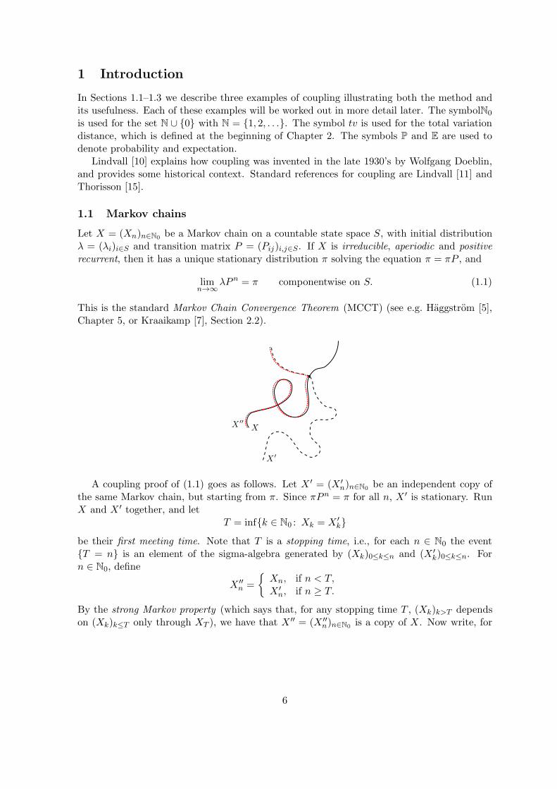
A coupling proof of (1.1) goes as follows. Let X ′ = (X ′n)n∈N0
be an independent copy ofthe same Markov chain, but starting from π. Since πPn = π for all n, X ′ is stationary. RunX and X ′ together, and let
T = infk ∈ N0 : Xk = X ′k
be their first meeting time. Note that T is a stopping time, i.e., for each n ∈ N0 the eventT = n is an element of the sigma-algebra generated by (Xk)0≤k≤n and (X ′
k)0≤k≤n. Forn ∈ N0, define
X ′′n =
Xn, if n < T,X ′
n, if n ≥ T.By the strong Markov property (which says that, for any stopping time T , (Xk)k>T dependson (Xk)k≤T only through XT ), we have that X ′′ = (X ′′
n)n∈N0is a copy of X. Now write, for
6
i ∈ S,
(λPn)i − πi = P(X ′′n = i)− P(X ′
n = i)
= P(X ′′n = i, T ≤ n) + P(X ′′
n = i, T > n)
−P(X ′n = i, T ≤ n)− P(X ′
n = i, T > n)
= P(X ′′n = i, T > n)− P(X ′
n = i, T > n),
where we use P as the generic symbol for probability (in later Chapters we will be more carefulwith the notation). Hence
‖λPn − π‖tv =∑
i∈S|(λPn)i − πi|
≤∑
i∈S
[P(X ′′
n = i, T > n) + P(X ′n = i, T > n)
]= 2P(T > n).
The left-hand side is the total variation norm of λPn − π. The conditions in the MCCTguarantee that P(T <∞) = 1 (as will be explained in Chapter 6). The latter is expressed bysaying that the coupling is successful. Hence the claim in (1.1) follows by letting n→∞.
1.2 Birth-Death processes
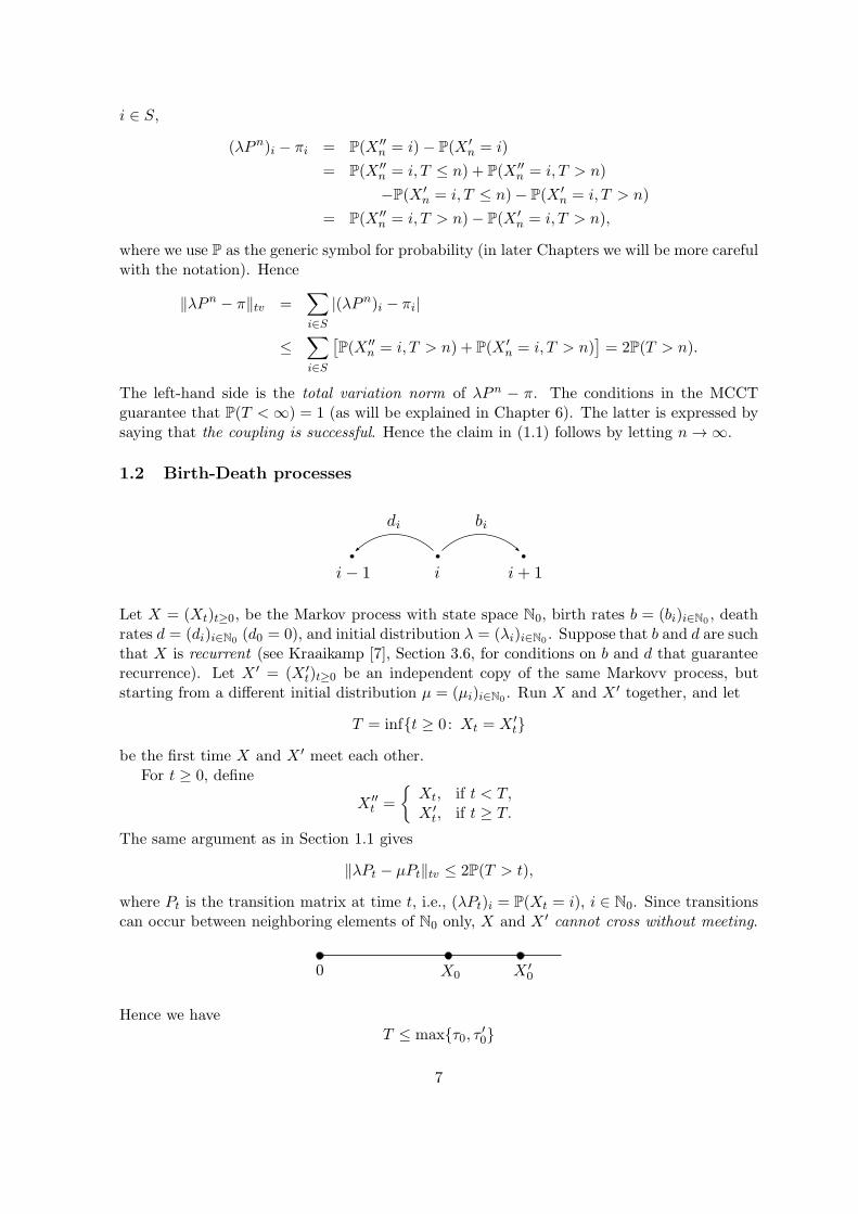
Let X = (Xt)t≥0, be the Markov process with state space N0, birth rates b = (bi)i∈N0, death
rates d = (di)i∈N0(d0 = 0), and initial distribution λ = (λi)i∈N0
. Suppose that b and d are suchthat X is recurrent (see Kraaikamp [7], Section 3.6, for conditions on b and d that guaranteerecurrence). Let X ′ = (X ′
t)t≥0 be an independent copy of the same Markovv process, butstarting from a different initial distribution µ = (µi)i∈N0
. Run X and X ′ together, and let
T = inft ≥ 0: Xt = X ′t
be the first time X and X ′ meet each other.For t ≥ 0, define
X ′′t =
Xt, if t < T,X ′
t, if t ≥ T.The same argument as in Section 1.1 gives
‖λPt − µPt‖tv ≤ 2P(T > t),
where Pt is the transition matrix at time t, i.e., (λPt)i = P(Xt = i), i ∈ N0. Since transitionscan occur between neighboring elements of N0 only, X and X ′ cannot cross without meeting.
Hence we haveT ≤ maxτ0, τ ′0
7
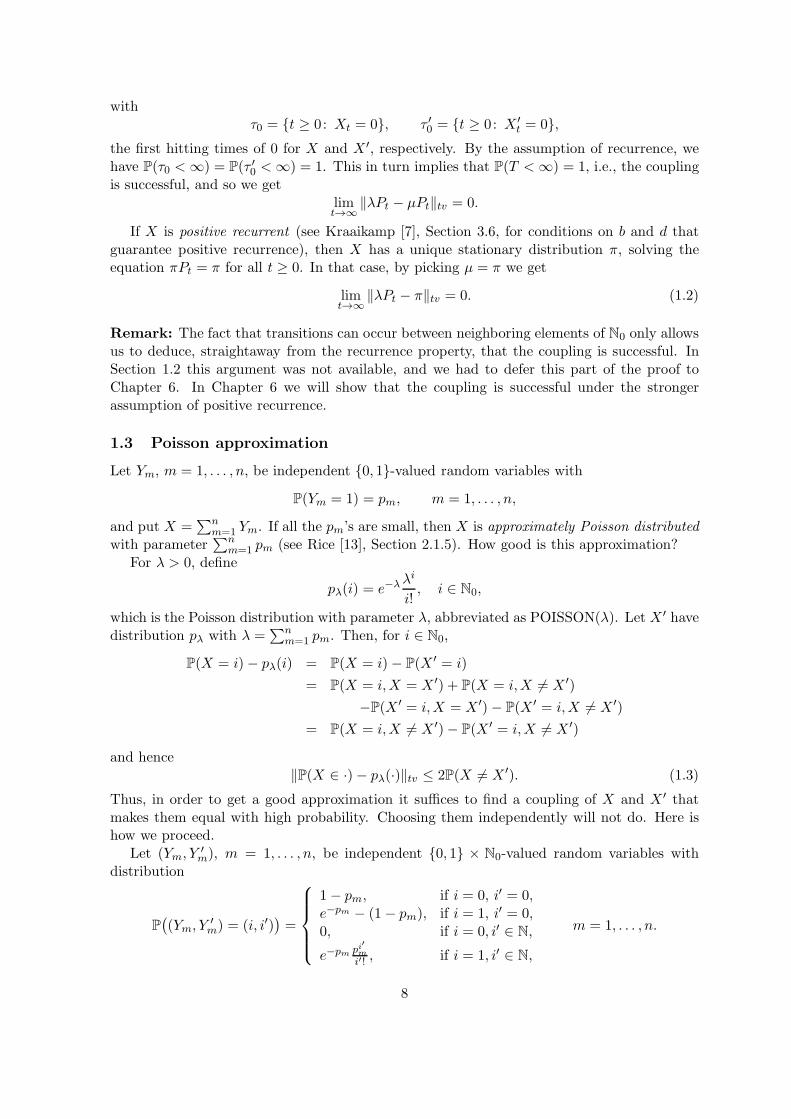
withτ0 = t ≥ 0: Xt = 0, τ ′0 = t ≥ 0: X ′
t = 0,the first hitting times of 0 for X and X ′, respectively. By the assumption of recurrence, wehave P(τ0 <∞) = P(τ ′0 <∞) = 1. This in turn implies that P(T <∞) = 1, i.e., the couplingis successful, and so we get
limt→∞
‖λPt − µPt‖tv = 0.
If X is positive recurrent (see Kraaikamp [7], Section 3.6, for conditions on b and d thatguarantee positive recurrence), then X has a unique stationary distribution π, solving theequation πPt = π for all t ≥ 0. In that case, by picking µ = π we get
limt→∞
‖λPt − π‖tv = 0. (1.2)
Remark: The fact that transitions can occur between neighboring elements of N0 only allowsus to deduce, straightaway from the recurrence property, that the coupling is successful. InSection 1.2 this argument was not available, and we had to defer this part of the proof toChapter 6. In Chapter 6 we will show that the coupling is successful under the strongerassumption of positive recurrence.
1.3 Poisson approximation
Let Ym, m = 1, . . . , n, be independent 0, 1-valued random variables with
P(Ym = 1) = pm, m = 1, . . . , n,
and put X =∑n
m=1 Ym. If all the pm’s are small, then X is approximately Poisson distributedwith parameter
∑nm=1 pm (see Rice [13], Section 2.1.5). How good is this approximation?
For λ > 0, define
pλ(i) = e−λλi
i!, i ∈ N0,
which is the Poisson distribution with parameter λ, abbreviated as POISSON(λ). Let X ′ havedistribution pλ with λ =
∑nm=1 pm. Then, for i ∈ N0,
P(X = i)− pλ(i) = P(X = i)− P(X ′ = i)
= P(X = i,X = X ′) + P(X = i,X 6= X ′)
−P(X ′ = i,X = X ′)− P(X ′ = i,X 6= X ′)
= P(X = i,X 6= X ′)− P(X ′ = i,X 6= X ′)
and hence‖P(X ∈ ·)− pλ(·)‖tv ≤ 2P(X 6= X ′). (1.3)
Thus, in order to get a good approximation it suffices to find a coupling of X and X ′ thatmakes them equal with high probability. Choosing them independently will not do. Here ishow we proceed.
Let (Ym, Y′m), m = 1, . . . , n, be independent 0, 1 × N0-valued random variables with
distribution
P((Ym, Y
′m) = (i, i′)
)=
1− pm, if i = 0, i′ = 0,e−pm − (1− pm), if i = 1, i′ = 0,0, if i = 0, i′ ∈ N,
e−pm pi′m
i′! , if i = 1, i′ ∈ N,
m = 1, . . . , n.
8
By summing out over i′, respectively, i we see that
P(Ym = i) =
1− pm, if i = 0,pm, if i = 1,
P(Y ′m = i′) = e−pm p
i′m
i′!, i′ ∈ N0,
so that the marginal distributions are indeed correct and we have a proper coupling. Nowestimate
P(X 6= X ′) = P
(n∑
m=1
Ym 6=n∑
m=1
Y ′m
)
≤ P(∃m ∈ 1, . . . , n : Ym 6= Y ′
m
)
≤n∑
m=1
P(Ym 6= Y ′m)
=n∑
m=1
[e−pm − (1− pm) +
∞∑
i′=2
e−pm pi′m
i′!
]
=
n∑
m=1
pm(1− e−pm)
≤n∑
m=1
p2m.
Hence, for λ =∑n
m=1 pm, we have proved that
‖P(X ∈ ·)− pλ(·)‖tv ≤ 2λM
with M = maxm=1,...,n pm. This quantifies the extent to which the approximation is goodwhen M is small. Both λ and M will in general depend on n. Typical applications will haveλ of order 1 and M tending to zero as n→∞.
Remark: The coupling produced above will turn out to be the best possible: it is a maximalcoupling (see Chapter 2.5). The crux is that (Ym, Y
′m) = (0, 0) and (1, 1) are given the largest
possible probabilities. More details will be given in Chapter 5.
9
2 Basic theory of coupling
Chapters 2 and 7 provide the theoretical basis for the theory of coupling and consequently aretechnical in nature. It is here that we arm ourselves with a number of basic facts about couplingthat are needed to deal with the applications described in Chapters 3–6 and Chapters 8–10. InSection 2.1 we give the definition of a coupling of two probability measures, in Section 2.2 westate and derive the basic coupling inequality, bounding the total variation distance betweentwo probability measures in terms of their coupling time, in Section 2.3 we look at boundson the coupling time of two random sequences, in Section 2.4 we introduce the notion ofdistributional coupling, while in Section 2.5 we prove the existence of a maximal coupling forwhich the coupling inequality is optimal.
In what follows we use some elementary ingredients from measure theory, for which werefer the reader to standard textbooks.
Definition 2.1 Given a bounded signed measure M on a measurable space (E, E) such thatM(E) = 0, the total variation norm of M is defined as
‖M‖tv = 2 supA∈E
M(A).
Remark: The total variation norm of M is defined as
‖M‖tv = sup‖f‖∞≤1
∣∣∣∣∫
Ef dM
∣∣∣∣ ,
where the supremum runs over all functions f : E → R that are bounded and measurable w.r.t.E , and ‖f‖∞ = supx∈E |f(x)| is the supremum norm. By the Jordan-Hahn decompositiontheorem, there exists a set D ∈ E such that M+(·) = M( · ∩D) and M−(·) = −M( · ∩Dc) areboth non-negative measures on (E, E). Clearly, M = M+ −M− and supA∈E M(A) = M(D) =M+(E). It therefore follows that ‖M‖tv =
∫E(1D − 1Dc) dM = M+(E) +M−(E) (note that
the absolute value sign disappears). If M(E) = 0, then M+(E) = M−(E), in which case‖M‖tv = 2M+(E) = 2 supA∈E M(A).
2.1 Definition of coupling
A probability space is a triple (E, E ,P), with (E, E) a measurable space consisting of a samplespace E and a σ-algebra E of subsets of E, and with P a probability measure on E . Typically,E is a Polish space (i.e., complete, separable and metric) and E consists of its Borel sets.
Definition 2.2 A coupling of two probability measures P and P′ on the same measurable space(E, E) is any (!) probability measure P on the product measurable space (E×E, E ⊗E) (whereE ⊗ E is the smallest sigma-algebra containing E × E) whose marginals are P and P′, i.e.,
P = P π−1, P′ = P π′−1,
where π is the left-projection and π′ is the right-projection, defined by
π(x, x′) = x, π′(x, x′) = x′, (x, x′) ∈ E × E.A similar definition holds for random variables. Given a probability space (Ω,F ,Q), a
random variable X is a measurable mapping from (Ω,F) to (E, E). The image of Q underX is P, the probability measure of X on (E, E). When we are interested in X only, we mayforget about (Ω,F ,Q) and work with (E, E ,P) only.
10
Definition 2.3 A coupling of two random variable X and X ′ taking values in (E, E) is any(!) pair of random variables (X, X ′) taking values in (E × E, E ⊗ E) whose marginals havethe same distribution as X and X ′, i.e.,
XD=X, X ′ D=X ′,
withD= denoting equality in distribution.
Remark: The law P of (X, X ′) is a coupling of the laws P,P′ of X,X ′ in the sense ofDefinition 2.2.
Remark: Couplings are not unique. Two trivial examples are:
P = P× P′ with P,P′ arbitrary ⇐⇒ X, X ′ are independent,
P = P′ and P lives on the diagonal ⇐⇒ X = X ′.
Non-trivial examples were given in Chapter 1.
In applications the challenge is to find a coupling that makes ‖P−P′‖tv as small as possible.For this reason coupling is an art, not a recipe. We will see plenty of examples as we go along.
2.2 Coupling inequalities
2.2.1 Random variables
The basic coupling inequality for two random variables X,X ′ with probability distributionsP,P′ reads as follows:
Theorem 2.4 Given two random variables X,X ′ with probability distributions P,P′, any (!)coupling P of P,P′ satisfies
‖P− P′‖tv ≤ 2P(X 6= X ′).
Proof. Pick any A ∈ E and write
P(X ∈ A)− P′(X ′ ∈ A) = P(X ∈ A)− P(X ′ ∈ A)= P(X ∈ A, X = X ′) + P(X ∈ A, X 6= X ′)
−P(X ′ ∈ A, X = X ′)− P(X ′ ∈ A, X 6= X ′)
= P(X ∈ A, X 6= X ′)− P(X ′ ∈ A, X 6= X ′).
Hence, by Definition 2.1 (where we write P(A) = P(X ∈ A)),
‖P− P′‖tv = 2 supA∈E
[P(A)− P′(A)]
= 2 supA∈E
[P(X ∈ A)− P′(X ′ ∈ A)]
≤ 2 supA∈E
P(X ∈ A, X 6= X ′)
= 2P(X 6= X ′),
where the last equality holds because the supremum is achieved at A = E ∈ E .
11
Exercise 2.5 Let U, V be random variables on N0 with probability mass functions
fU(x) =12 10,1(x), fV (x) =
13 10,1,2(x), x ∈ N0,
where 1S is the indicator function of the set S. (a) Compute the total variation distance.(b) Give two different couplings of U and V . (c) Give a coupling of U and V under whichU ≥ V with probability 1.
Exercise 2.6 Let U, V be random variables on [0,∞) with probability density functions
fU (x) = 2e−2x, fV (x) = e−x, x ∈ [0,∞).
Answer the same questions as in Exercise 2.5.
2.2.2 Sequences of random variables
There is also a version of the coupling inequality for sequences of random variables. LetX = (Xn)n∈N0
and X ′ = (X ′n)n∈N0
be two sequences of random variables taking values in(EN0 , E⊗N0). Let (X, X ′) be a coupling of X and X ′. Define
T = infn ∈ N0 : Xm = X ′m for all m ≥ n,
which is the coupling time of X and X ′, i.e., the first time from which the two sequences agreeonwards (possibly T =∞).
Theorem 2.7 For two sequences of random variables X = (Xn)n∈N0and X ′ = (X ′
n)n∈N0
taking values in (EN0 , E⊗N0), let (X, X ′) be a coupling of X and X ′, and let T be the couplingtime. Then
‖P(Xn ∈ ·)− P′(Xn ∈ ·)‖tv ≤ 2P(T > n).
Proof. This follows from Theorem 2.4 because Xn 6= X ′n ⊆ T > n.
Remark: In Section 1.3 we already saw an example of sequence coupling, namely, X andX ′ were two copies of a Birth-Death process starting from different initial distributions. TheMarkov property implies that T is equal in distribution to the first time X and X ′ meet eachother.
A stronger form of sequence coupling can be obtained by introducing the left-shift θ onEN0 , defined by
θ(x0, x1, . . .) = (x1, x1, . . .),
i.e., θ drops the first element of the sequence.
Theorem 2.8 Let X, X ′ and T be defined as in Theorem 2.7. Then
‖P(θnX ∈ ·)− P′(θnX ′ ∈ ·)‖tv ≤ 2P(T > n).
Proof. BecauseXm 6= X ′
m for some m ≥ n ⊆ T > n,the claim again follows from Theorem 2.4.
Remark: Similar inequalities hold for continuous-time random processes X = (Xt)t≥0 andX ′ = (X ′
t)t≥0.
12
2.2.3 Mappings
Since total variation distance never increases under a mapping, we have the following corollary.
Corollary 2.9 Let ψ be a measurable map from (E, E) to (E∗, E∗). Let Q = P ψ−1 andQ′ = P′ ψ−1 (i.e., Q(B) = P(ψ−1(B)) and Q′(B) = P′(ψ−1(B)) for B ∈ E∗). Then
‖Q−Q′‖tv ≤ ‖P− P′‖tv ≤ 2P(X 6= X ′).
Proof. Simply estimate
‖Q −Q′‖tv = 2 supB∈E∗
[Q(B)−Q′(B)]
= 2 supB∈E∗
[P(ψ(X) ∈ B)− P′(ψ(X ′) ∈ B)]
≤ 2 supA∈E
[P(X ∈ A)− P′(X ′ ∈ A)] (A = ψ−1(B))
= ‖P− P′‖tv ,
where the inequality comes from the fact that E may be larger than ψ−1(E∗). Use Theorem 2.4to get the bound.
2.3 Rates of convergence
Suppose that we have some control on the moments of the coupling time T , e.g. for someφ : N0 → [0,∞) non-decreasing with limn→∞ φ(n) =∞ we know that
E(φ(T )) <∞.
Theorem 2.10 Let X,X ′ and φ be as above. Then
‖P(θnX ∈ ·)− P′(θnX ′ ∈ ·)‖tv = o(1/φ(n)
)as n→∞.
Proof. Estimateφ(n) P(T > n) ≤ E
(φ(T )1T>n
).
Note that the right-hand side tends to zero as n → ∞ by dominated convergence, becauseE(φ(T )) <∞. Use Theorem 2.8 to get the claim.
Typical examples are:
φ(n) = nα, α > 0 (polynomial rate),φ(n) = eβn, β > 0 (exponential rate).
For instance, for finite-state irreducible aperiodic Markov chains, there exists an M <∞ suchthat P(T > 2M | T > M) ≤ 1
2 (see Haggstrom [5], Chapter 5), which implies that there exists
a β > 0 such that E(eβT ) < ∞. In Section 3 we will see that for random walks we typicallyhave E(Tα) <∞ for all 0 < α < 1
2 .
13
2.4 Distributional coupling
Suppose that a coupling (X, X ′) of two random sequences X = (Xn)n∈N0and X ′ = (X ′
n)n∈N0
comes with two random times T and T ′ such that not only
XD=X, X ′ D=X ′,
but also (θT X, T
) D=(θT
′X ′, T ′).
Here we compare the two sequences shifted over different random times, rather than the samerandom time.
Theorem 2.11 Let X, X ′, T , T ′ be as above. Then
‖P(θnX ∈ ·)− P′(θnX ′ ∈ ·)‖tv ≤ 2P(T > n)[= 2P(T ′ > n)
].
Proof. Write, for A ∈ E⊗N0 ,
P(θnX ∈ A,T ≤ n) =n∑
m=0
P(θn−m(θmX) ∈ A,T = m)
=
n∑
m=0
P(θn−m(θmX ′) ∈ A,T ′ = m)
= P(θnX ′ ∈ A,T ′ ≤ n).
It follows that
P(θnX ∈ A)− P(θnX ′ ∈ A) = P(θnX ∈ A,T > n)− P(θnX ′ ∈ A,T ′ > n)
≤ P(T > n),
and hence
‖P(θnX ∈ ·)− P′(θnX ′ ∈ ·)‖tv = 2 supA∈E⊗N0
[P(θnX ∈ A)− P′(θnX ′ ∈ A)]
= 2 supA∈E⊗N0
[P(θnX ∈ A)− P(θnX ′ ∈ A)]
≤ 2P(T > n).
Remark: A restrictive feature of distributional coupling is that TD=T ′, i.e., the two ran-
dom times must have the same distribution. Therefore distributional coupling is more of atheoretical than a practical tool. We will see in Chapter 4 that it plays a role in card shuffling.
Remark: In Section 6.2 we will encounter yet another form of coupling, called shift-coupling.This requires the existence of random times T, T ′ such that
θTX = θT′X ′
(which is stronger than θTXD= θT
′X ′), but does not require that T
D=T ′. This form of coupling
is useful for dealing with time averages. Thorisson [15] contains a critical analysis of howdifferent forms of coupling compare with each other.
14
2.5 Maximal coupling
Does there exist a “best possible” coupling, one that gives the sharpest estimate on the totalvariation distance, in the sense that the inequality in Theorem 2.4 becomes an equality? Theanswer is yes!
Theorem 2.12 For any two probability measures P and P′ on a measurable space (E, E) thereexists a coupling P such that
(i) ‖P− P′‖tv = 2P(X 6= X ′).
(ii) X and X ′ are independent conditional on X 6= X ′, provided the latter event haspositive probability.
Proof. We give an abstract construction of a maximal coupling. Let ∆ = (x, x) : x ∈ E bethe diagonal of E × E. Let ψ : E → E × E be the map defined by ψ(x) = (x, x).
Exercise 2.13 Show that ψ is measurable because E is a Polish.
Put
λ = P+ P′, g =dP
dλ, g′ =
dP′
dλ,
and note that g and g′ are well defined because P and P′ are both absolutely continuous w.r.t.λ. Define Q on (E, E) and Q on (E × E, E ⊗ E) by
dQ
dλ= g ∧ g′, Q = Q ψ−1.
(Both are sub-probability measures.) Then Q puts all its mass on ∆. Call this mass γ = Q(∆),and put
ν = P−Q, ν ′ = P′ −Q, P =ν × ν ′1− γ + Q.
Then
P(A× E) =ν(A)× ν ′(E)
1− γ + Q(A× E) = P(A),
because ν(A) = P(A)−Q(A), ν ′(E) = P′(E)−Q(E) = 1−γ and Q(A×E) = Q(A). Similarly,P(E ×A) = P′(A), so that the marginals are indeed correct and we have a proper coupling.
To get (i), compute
‖P− P′‖tv =
∫
E|g − g′| dλ = 2
[1−
∫
E(g ∧ g′) dλ
]
= 2 [1−Q(E)] = 2(1 − γ) = 2P(∆c) = 2P(X 6= X ′).
Here, the first equality uses the Jordan-Hahn decomposition of signed measures into a differ-ence of non-negative measures, the second equality uses the identity |g−g′| = g+g′−2(g∧g′),the third equality uses the definition of Q, the fourth equality uses that Q(E) = Q(∆) = γ,the fifth equality uses that Q(∆c) = 0 and (ν × ν ′)(∆c) = ν(E)ν ′(E) = (1 − γ)2, while thesixth equality uses the definition of ∆.
Exercise 2.14 Prove the first equality. Hint: use a splitting as in the remark below Defini-tion 2.1 with M = P− P′ and D = x ∈ E : g(x) ≥ g′(x).
15
To get (ii), note that
P( · | X 6= X ′) = P( · | ∆c) =
(ν
1− γ ×ν ′
1− γ
)(·).
Remark: What Theorem 2.12 says is that we can in principle find a coupling that gives thecorrect value for the total variation. Such a coupling is called a maximal coupling. However, inpractice it is often difficult to write out this coupling explicitly (the above is only an abstractconstruction), and we have to content ourselves with good estimates or approximations. Wewill encounter examples in Chapter 9.
Exercise 2.15 Give a maximal coupling of U and V in Exercise 2.5.
Exercise 2.16 Give a maximal coupling of U and V in Exercise 2.6.
Exercise 2.17 Is the coupling of the two coins in PRELUDE 2 a maximal coupling?
16
3 Random walks
Random walks on Zd, d ≥ 1, are special cases of Markov chains: the transition probability togo from site x to site y only depends on the difference vector y−x. Because of this translationinvariance, random walks can be analyzed in great detail. A standard reference is Spitzer [14].One key fact we will use below is that any irreducible random walk whose step distributionhas zero mean and finite variance is recurrent in d = 1, 2 and transient in d ≥ 3. In d = 1 anyrandom walk whose step distribution has zero mean and finite first moment is recurrent.
In Section 3.1 we look at random walks in dimension 1, in Section 3.2 at random walksin dimension d. In Section 3.3 we use random walks in dimension d to show that boundedharmonic functions on Zd are constant. This result has an interesting interpretation in physics:a system in thermal equilibrium has a constant temperature.
3.1 Random walks in dimension 1
3.1.1 Simple random walk
Let S = (Sn)n∈N0be a simple random walk on Z starting at 0, i.e., S0 = 0 and Sn =
∑ni=1 Yi,
n ∈ N, where Y = (Yi)i∈N are i.i.d. with
P(Yi = −1) = P(Yi = 1) = 12 .
The following theorem says that, modulo period 2, the distribution of Sn becomes flat forlarge n.
Theorem 3.1 Let S be a simple random walk. Then, for every k ∈ Z even,
limn→∞
‖P(Sn ∈ · )− P(Sn + k ∈ · )‖tv = 0.
Proof. Let S′ denote an independent copy of S starting at S′0 = k. Write P for the joint
probability distribution of (S, S′), and let
T = minn ∈ N0 : Sn = S′n.
Then‖P(Sn ∈ · )− P(Sn + k ∈ · )‖tv = ‖P(Sn ∈ · )− P(S′
n ∈ · )‖tv ≤ 2P(T > n).
Now, S = (Sn)n∈N0defined by Sn = S′
n − Sn is a random walk on Z starting at S0 = k withi.i.d. increments Y = (Yi)i∈N given by
P(Yi = −2) = P(Yi = 2) = 14 , P(Yi = 0) = 1
2 .
This is a simple random walk on 2Z with a “random time delay”, namely, it steps only halfof the time. Since
T = τ0 = n ∈ N0 : Sn = 0and k is even, it follows from the recurrence of S that P(T <∞) = 1. Let n→∞ to get theclaim.
In analytical terms, Theorem 3.1 says the following. Let p(·, ·) denote the transition kernelof the simple random walk, let pn(·, ·), n ∈ N, denote the n-fold composition of p(·, ·), and
17
let δk(·), k ∈ Z, denote the vector whose components are 1 at k and 0 elsewhere. ThenTheorem 3.1 says that for k even
limn→∞
‖δkpn(·) − δ0pn(·)‖tv = 0.
(This short-hand notation comes from the fact that δkpn(·) = P(Sn ∈ · | S0 = k).) It
is possible to prove the latter statement by hand, i.e., by computing δkpn(·) and δ0p
n(·),evaluating their total variation distance and letting n→∞. However, this computation turnsout to be somewhat involved.
Exercise 3.2 Do the computation. Hint: Use the formula
δkpn(l) = (12)
n
(n
12(n+ |k − l|)
), k, l ∈ Z, n+ |k − l| even.
The result in Theorem 3.1 cannot be extended to k odd. In fact, because the simplerandom walk has period 2, the laws of Sn and Sn + k have disjoint support when k is odd,irrespective of n, and so
‖P(Sn ∈ · )− P(Sn + k ∈ · )‖tv = 2 ∀n ∈ N0, k ∈ Z odd.
3.1.2 Beyond simple random walk
Does the same result as in Theorem 3.1 hold for random walks other than the simple randomwalk? Yes, it does! To formulate the appropriate statement, let S be the random walk on Z
with i.i.d. increments Y satisfying the aperiodicity condition
gcdz′ − z : z, z′ ∈ Z, P(Y1 = z)P(Y1 = z′) > 0
= 1. (3.1)
Theorem 3.3 Subject to (3.1),
limn→∞
‖P(Sn ∈ · )− P(Sn + k ∈ · )‖tv = 0 ∀ k ∈ Z.
Proof. We try to use the same coupling as in the proof of Theorem 3.1. Namely, we putSn = S′
n − Sn, n ∈ N0, we note that S = (Sn)n∈N0is a random walk starting at S0 = k whose
i.i.d. increments Y = (Yi)i∈N are given by
P(Y1 = z) =∑
z,z′∈Z
z′−z=z
P(Y1 = z)P(Y1 = z′), z ∈ Z,
we further note that (3.1) written in terms of P transforms into
gcdz ∈ Z : P(Y1 = z) > 0 = 1, (3.2)
so that S is an aperiodic random walk, and finally we argue that S is recurrent, i.e.,
P(τ0 <∞) = 1,
to complete the proof. However, there is a problem: recurrence may fail ! Indeed, even thoughS is a symmetric random walk (because P(Y1 = z) = P(Y1 = −z), z ∈ Z), the distribution of
18
Y1 may have a thick tail resulting in E(|Y1|) =∞, in which case S is not necessarily recurrent(see Spitzer [14], Section 3).
The lack of recurrence may be circumvented by slightly adapting the coupling. Namely,instead of letting the two copies of the random walk S and S′ step independently, we letthem make independent small steps, but dependent large steps. Formally, we let Y ′′ be anindependent copy of Y , and we define Y ′ by putting
Y ′i =
Y ′′i if |Yi − Y ′′
i | ≤ N,Yi if |Yi − Y ′′
i | > N,(3.3)
i.e., S′ copies the jumps of S′′ when they differ from the jumps of S by at most N , otherwiseS′ copies the jumps of S. The value of N ∈ N is arbitrary and will later be taken large enough.
First, we check that S′ is a copy of S. This is so because, for every z ∈ Z,
P′(Y ′1 = z) = P(Y ′
1 = z, |Y1 − Y ′′1 | ≤ N) + P(Y ′
1 = z, |Y1 − Y ′′1 | > N)
= P(Y ′′1 = z, |Y1 − Y ′′
1 | ≤ N) + P(Y1 = z, |Y1 − Y ′′1 | > N),
and the first term in the right-hand side equals P(Y1 = z, |Y1 − Y ′′1 | ≤ N) by symmetry (use
that Y and Y ′′ are independent), so that we get P′(Y ′1 = z) = P(Y1 = z).
Next, we note from (3.3) that the difference random walk S = S − S′ has increments
Yi = Y ′i − Yi =
Y ′′i − Yi if |Yi − Y ′′
i | ≤ N,0 if |Yi − Y ′′
i | > N,
i.e., no jumps larger than N can occur. Moreover, by picking N large enough we also havethat
P(Y1 6= 0) > 0 and (3.2) holds.
Exercise 3.4 Prove the last two statements.
Thus, S is an aperiodic symmetric random walk on Z with bounded step size. Consequently,S is recurrent and therefore we have P(τ0 <∞) = 1, so that the proof of Theorem 3.3 can becompleted in the same way as the proof of Theorem 3.1.
Remark: The coupling in (3.3) is called the Ornstein coupling. The idea is that S′ managesto stay close to S by copying its large jumps.
Remark: Theorem 3.1 may be sharpened by noting that
P(T > n) = O
(1√n
).
Indeed, this follows from a classical result for random walks in d = 1 with zero mean andfinite variance, namely P(τz > n) = O( 1√
n) for all z 6= 0 with τz the first hitting time of z (see
Spitzer [14], Section 3). Consequently,
‖P(Sn ∈ · )− P(Sn + k ∈ · )‖tv = O
(1√n
)∀ k ∈ Z even.
A direct proof of this estimate without coupling turns out to be rather hard, especially foran arbitrary random walk in d = 1 with zero mean and finite variance. Even a well-trainedanalyst typically does not manage to cook up a proof in a day! Exercise 3.2 shows how toproceed for simple random walk.
Exercise 3.5 Show that, without (3.1), Theorem 3.3 holds if and only if k is a multiple ofthe period.
19
3.2 Random walks in dimension d
Question: What about random walks on Zd, d ≥ 2? We know that an arbitrary irreduciblerandom walk in d ≥ 3 is transient, and so the Ornstein coupling does not work to bring thetwo coupled random walks together with probability 1.
Answer: It still works, provided we do the Ornstein coupling componentwise.
3.2.1 Simple random walk
Here is how the componentwise coupling works. We first consider a simple random walk onZd, d ≥ 2. Pick direction 1, i.e., look at the x1-coordinate of the random walks S and S′, andcouple these as follows:
Yi ∈ −e1, e1 =⇒ draw Y ′i ∈ −e1, e1 independently with probability 1
2 each,
Yi /∈ −e1, e1 =⇒ put Y ′i = Yi.
The difference random walk S = S′ − S has increments Y given by
P(Yi = −2e1) = P(Yi = 2e1) =(
12d
)2, P(Yi = 0) = 1− 2
(12d
)2.
Start at S0 = z ∈ Zd with all components z1, . . . , zd even, and use that S is recurrent indirection 1, to get that
τ1 = infn ∈ N0 : S1n = 0
satisfies P(τ1 <∞). At time τ1 change the coupling to direction 2, i.e., do the same but nowidentify the steps in all directions different from 2 and allow for independent steps only indirection 2. Put
τ2 = infn ≥ τ1 : S2n = 0
and note that P(τ2 − τ1 <∞) = 1. Continue until all d directions are exhausted. At time
τd = infn ≥ τd−1 : Sdn = 0,
for which P(τd − τd−1 < ∞) = 1, the two walks meet. Since P(τd < ∞) = 1, the coupling issuccessful and the proof is complete.
To get the same result when z1 + · · · + zd is even (rather than all z1, . . . , zd being even),we argue as follows. There is an even number of directions i for which zi is odd. Pairthese directions in an arbitrary manner, say, (i1, j1), . . . , (il, jl) for some 1 ≤ l ≤ d. Doa componentwise coupling in the directions (i1, j1), i.e., the jumps of S in direction i1 areindependent of the jumps of S′ in direction j1, while the jumps in all directions other than i1and j1 are copied. Wait until S′− S is even in directions i1 and j1, switch to the pair (i2, j2),etc., until all components of S′ − S are even. After that do the componentwise coupling asbefore.
Exercise 3.6 Write out the details of the last argument.
3.2.2 Beyond simple random walk
The general statement is as follows. Suppose thatz′ − z : z, z′ ∈ Zd, P(Y1 = z)P(Y1 = z′) > 0
is not contained in any sublattice of Zd, (3.4)
which is the analogue of (3.1).
20
Theorem 3.7 Subject to (3.4),
limn→∞
‖P(Sn ∈ · )− P(Sn + z ∈ · )‖tv = 0 ∀ z ∈ Zd.
Proof. Combine the componentwise coupling with the “cut out large steps” in the Ornsteincoupling (3.3).
Exercise 3.8 Write out the details of the proof. Warning: The argument is easy when therandom walk can move in only one direction at a time (like simple random walk). For otherrandom walks a projection argument is needed.
Exercise 3.9 Show that, without (3.4), Theorem 3.7 holds if and only if z is an element ofthe minimal sublattice containing
z′ − z : z, z′ ∈ Zd, P(Y1 = z)P(Y1 = z′) > 0
.
3.3 Random walks and the discrete Laplacian
The result in Theorem 3.7 has an interesting corollary. Let ∆ denote the discrete Laplacianacting on functions f : Zd → R as
(∆f)(x) =1
2d
∑
y∈Zd
‖y−x‖=1
[f(y)− f(x)], x ∈ Zd.
A function f is called harmonic when ∆f ≡ 0, i.e., f is at every site equal to the average ofits values at neighboring sites.
Theorem 3.10 All bounded harmonic functions on Zd are constant.
Proof. Let S be a simple random walk starting at 0. Then, by the harmonic property of f ,we have
E(f(Sn)) = E(E(f(Sn) | Sn−1)
)= E(f(Sn−1)),
where we use that E(f(Sn) | Sn−1 = x) = f(x) + (∆f)(x) = f(x). Iteration gives E(f(Sn)) =f(0). Now pick any x, y ∈ Zd such that all components of x− y are even, and estimate
|f(x)− f(y)| = |E(f(Sn + x))− E(f(Sn + y))|
=∣∣∣∑
z∈Zd
[f(z + x)− f(z + y)]P(Sn = z)∣∣∣
=∣∣∣∑
z∈Zd
f(z)[P(Sn = z − x)− P(Sn = z − y)
]∣∣∣
≤ M∑
z∈Zd
|P(Sn + x = z)− P(Sn + y = z)|
= M‖P(Sn + x ∈ · )− P(Sn + y ∈ · )‖tv
with M = supz∈Zd |f(z)| <∞. Let n→∞ and use Theorem 3.7 to get f(x) = f(y). Extendthis equality to x, y ∈ Zd with ‖x− y‖ even by first doing the coupling in paired directions, asin Section 3.2. Hence we conclude that f is constant on the even and on the odd sublattice ofZd, say, f ≡ ceven and f ≡ codd. But codd = E(f(S1)) = f(0) = ceven, and so f is constant.
21
Remark: Theorem 3.10 has an interesting interpretation. Simple random walk can be used todescribe the flow of heat in a physical system. Space is discretized to Zd and time is discretizedto N0. Each site has a temperature that evolves with time according to the Laplace operator.Indeed, if x 7→ f(x) is the temperature profile at time n, then
x 7→ 1
2d
∑
y∈Zd
‖y−x‖=1
f(y) = f(x) + (∆f)(x)
is the temperature profile at time n+1: heat flows to neighboring sites proportionally to tem-perature differences. A temperature profile that is in equilibrium must therefore be harmonic,i.e., ∆f ≡ 0. Theorem 3.10 shows that on Zd the only temperature profile in equilibrium thatis bounded is the one where the temperature is constant.
Exercise 3.11 Give an example of an unbounded harmonic function on Z.
22
4 Card shuffling
Card shuffling is a topic that combines coupling, algebra and combinatorics. Diaconis [3] giveskey ideas. Levin, Peres and Wilmer [8] provides a broad panorama on mixing poperties ofMarkov chains, with Chapter 8 devoted to card shuffling. Two examples of random shufflesare described in the MSc-thesis by H. Nooitgedagt [12].
In Section 4.1 we present a general theory of random shuffles. In Section 4.2 we look ata specific random shuffle, called the “top-to-random shuffle”, for which we carry out explicitcomputations.
4.1 Random shuffles
Consider a deck with N ∈ N cards, labeled 1, . . . , N . An arrangement of the deck is anelement of the set PN of permutations of (1, . . . , N). We think of the first coordinate in thepermutation as the label of the “top card” and the last coordinate as the label of the “bottomcard”.
Definition 4.1 A shuffle of the deck is a permutation drawn from PN and applied to thedeck. A random shuffle is a shuffle drawn according to some probability distribution on PN .
Applying independent random shuffles to the deck, we get a Markov chainX = (Xn)n∈N0on
PN . If each shuffle uses the same probability distribution on PN , thenX is time-homogeneous.In typical cases, X is irreducible and aperiodic, with a unique invariant distribution π thatis uniform on PN . (The latter corresponds to a random shuffle that leads to a “randomdeck” after it is applied many times.) Since PN is finite, we know that the distribution of Xn
converges to π exponentially fast as n→∞, i.e.,
‖P(Xn ∈ · )− π(·)‖tv ≤ e−δn
for some δ = δ(N) > 0 and n ≥ n(N, δ).In what follows we will be interested in establishing a threshold time, written tN , around
which the total variation norm drops from being close to 2 to being close to 0, i.e., we want toidentify the time of approach to the invariant distribution (tN is also called a “mixing time”).
Definition 4.2 (tN )N∈N is called a sequence of threshold times if limN→∞ tN = ∞ and, forall ǫ > 0 small enough,
limN→∞
infn≤(1−ǫ)tN
‖P(Xn ∈ · )− π(·)‖tv = 2,
limN→∞
supn≥(1+ǫ)tN
‖P(Xn ∈ · )− π(·)‖tv = 0.
It turns out that for card shuffling threshold times typically grow with N in a polynomialfashion.
To capture the phenomenon of threshold time, we need the notion of strong uniform time.
Definition 4.3 T is a strong uniform time if the following hold:1. T is a stopping time, i.e., for all n ∈ N0 the event T = n is an element of the σ-algebraFn = σ(X0,X1, . . . ,Xn) containing all events that involve X up to time n.
2. XTD=π.
23
3. XT and T are independent.
Remark: Think of T = TN as the random time at which the random shuffling of the deckis stopped such that the arrangement of the deck is “completely random” (this is a form ofdistributional coupling defined in Section 2.4). In typical cases the threshold times (tN )N∈Nare such that
limN→∞
E(TN )/tN = 1, limN→∞
P(1− δ < TN/tN < 1 + δ) = 1 ∀ δ > 0. (4.1)
In Section 4.2 we will construct TN for a special example of a random shuffle.
Theorem 4.4 If T is a strong uniform time, then
‖P(Xn ∈ · )− π(·)‖tv ≤ 2P(T > n) ∀n ∈ N0.
Proof. By now the intuition behind this inequality should be obvious. For n ∈ N0 and A ⊂ PN ,write
P(Xn ∈ A,T ≤ n) =∑
σ∈PN
n∑
i=0
P(Xn ∈ A | Xi = σ, T = i)P(Xi = σ, T = i)
=
n∑
i=0
P(T = i)
∑
σ∈PN
P(Xn−i ∈ A | X0 = σ)π(σ)
=n∑
i=0
P(T = i) π(A)
= π(A)P(T ≤ n),where the second equality uses that P(Xn ∈ A | Xi = σ, T = i) = P(Xn−i ∈ A | X0 = σ)by the strong Markov property of X, and P(Xi = σ, T = i) = P(Xi = σ | T = i)P(T =i) = π(σ)P(T = i) by Definition 4.3, while the third equality holds because π is the invariantdistribution. Hence
P(Xn ∈ A)− π(A) = P(Xn ∈ A,T > n)− π(A)P(T > n)
=[P(Xn ∈ A | T > n)− π(A)
]P(T > n),
from which the claim follows after taking the supremum over A.
Remark: Note that T really is the coupling time to a parallel deck that starts in π, eventhough this deck is not made explicit.
4.2 Top-to-random shuffle
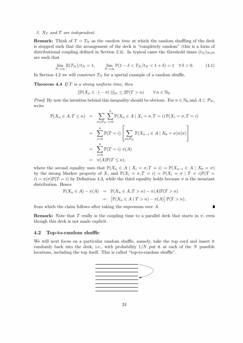
We will next focus on a particular random shuffle, namely, take the top card and insert itrandomly back into the deck, i.e., with probability 1/N put it at each of the N possiblelocations, including the top itself. This is called “top-to-random shuffle”.
24
Theorem 4.5 For the top-to-random shuffle the sequence (tN )N∈N with tN = N logN is asequence of threshold times.
Proof. Let T = τ∗ + 1, with
τ∗ = the first time that the original bottom card comes on top.
Exercise 4.6 Show that T is a strong uniform time. Hint: The +1 represents the insertionof the original bottom card at a random position in the deck after it has come on top.
For the proof it is convenient to view T differently, namely,
TD=V (4.2)
with V the number of random draws with replacement from an urn with N balls until eachball has been drawn at least once. To see why this holds, for i = 0, 1, . . . , N put
Ti = the first time there are i cards below the original bottom card,
Vi = the number of draws necessary to draw i distinct balls.
Then
Ti+1 − Ti D=VN−i − VN−(i+1)D=GEO
(i+ 1
N
), i = 0, 1 . . . , N − 1, are independent, (4.3)
where GEO(p) = p(1 − p)k−1 : k ∈ N denotes the geometric distribution with parameterp ∈ [0, 1].
Exercise 4.7 Prove (4.3).
Since T = TN =∑N−1
i=0 (Ti+1−Ti) and V = VN =∑N−1
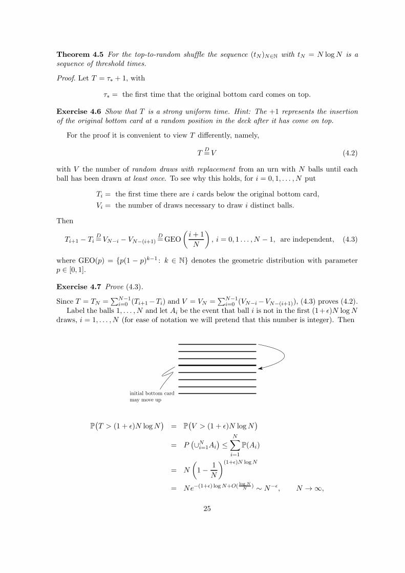
i=0 (VN−i−VN−(i+1)), (4.3) proves (4.2).Label the balls 1, . . . , N and let Ai be the event that ball i is not in the first (1+ ǫ)N logN
draws, i = 1, . . . , N (for ease of notation we will pretend that this number is integer). Then
P(T > (1 + ǫ)N logN
)= P
(V > (1 + ǫ)N logN
)
= P(∪Ni=1Ai
)≤
N∑
i=1
P(Ai)
= N
(1− 1
N
)(1+ǫ)N logN
= Ne−(1+ǫ) logN+O( logNN
) ∼ N−ǫ, N →∞,
25
which yields the second line of Definition 4.2 via Theorem 4.4.To get the first line of Definition 4.2, pick δ > 0, pick j = j(δ) so large that 1/j! < 1
2δ, anddefine
BN =σ ∈ PN : σN−j+1 < σN−j+2 < . . . < σN
= set of permutations whose last j terms are ordered upwards, N ≥ j.
Then π(BN ) = 1/j!, and Xn ∈ BN is the event that the order of the original j bottomcards is retained at time n. Since the first time the card with label N − j + 1 comes to thetop is distributed like VN−j+1, we have
P(X(1−ǫ)N logN ∈ BN
)≥ P
(VN−j+1 > (1− ǫ)N logN
). (4.4)
Indeed, for the upward ordering to be destroyed, the card with label N − j + 1 must come tothe top and must subsequently be inserted below the card with label N − j+1. We will showthat, for N ≥ N(δ),
P(VN−j+1 ≤ (1− ǫ)N logN
)< 1
2δ. (4.5)
From this it follows that∥∥P(X(1−ǫ)N logN) ∈ · )− π(·)
∥∥tv≥ 2
[P(X(1−ǫ)N logN) ∈ BN )− π(BN )
]
≥ 2[1− P
(VN−j+1 ≤ (1− ǫ)N logN
)− π(BN )
]
≥ 2 [1− 12δ − 1
2δ] = 2(1− δ).
The first inequality uses the definition of total variation, the third inequality uses (4.4) and(4.5). By letting N →∞ followed by δ ↓ 0, we get the first line of Definition 4.2.
To prove (4.5), we compute
E(VN−j+1) =
N−1∑
i=j−1
E(VN−i − VN−i−1)
=
N−1∑
i=j−1
N
i+ 1∼ N log
N
j∼ N logN
Var(VN−j+1) =N−1∑
i=j−1
Var(VN−i − VN−i−1)
=
N−1∑
i=j−1
(N
i+ 1
)2(1− i+ 1
N
)∼ cjN2, cj =
∑
k≥j
k−2.
Here we use that E(GEO(p)) = 1/p and Var(GEO(p)) = (1 − p)/p2. Chebyshev’s inequalitytherefore gives
P(VN−j+1 ≤ (1− ǫ)N logN
)= P
(VN−j+1 − E(VN−j+1) ≤ −ǫN logN [1 + o(1)]
)
≤ P([VN−j+1 − E(VN−j+1)]
2 ≥ ǫ2N2 log2N [1 + o(1)])
≤ Var(VN−j+1)
ǫ2E(VN−j+1)2[1 + o(1)]
∼ cjN2
ǫ2N2 log2N= O
(1
log2N
).
26
This proves (4.5).
Remark: We have shown that E(TN ) = 1 +∑N
i=1(N/i) ∼ N logN and Var(TN/E(TN ))→ 0as N →∞. This in turn implies that tN/TN → 1 in probability as N →∞ and identifies thescaling of the threshold time as tN ∼ E(TN ), in accordance with the prediction made in (4.1).
27
5 Poisson approximation
In Section 1.3 we already briefly described coupling in the context of Poisson approximation.We now return to this topic. Let BINOM(n, p) =
(nk
)pk(1 − p)n−k : k = 0, . . . , n be the
binomial distribution with parameters n ∈ N and p ∈ [0, 1]. A classical result from probabilitytheory is that, for every c ∈ (0,∞), BINOM(n, c/n) is close to POISSON(c) when n is large.In this section we will quantify how close, by developing a general theory for approximationsto the Poisson distribution called the Stein-Chen method. After suitable modification, thesame method also works for approximation to other types of distributions, e.g. the Gaussiandistribution, but this will not be pursued.
In Section 5.1 we derive a crude bound for sums of independent 0, 1-valued randomvariables. In Section 5.2 we describe the Stein-Chen method, which not only leads to a betterbound, but also applies to dependent random variables. In Section 5.3 we look at two specificapplications.
5.1 Coupling
Fix n ∈ N and p1, . . . , pn ∈ [0, 1). Let
YiD=BER(pi), i = 1, . . . , n, be independent,
i.e., P(Yi = 1) = pi and P(Yi = 0) = 1− pi, and put X =∑n
i=1 Yi.
Theorem 5.1 With the above definitions,
‖P(X ∈ · )− pλ(·)‖tv ≤n∑
i=1
λ2i
with λi = − log(1− pi), λ =∑n
i=1 λi and pλ = POISSON(λ).
Proof. Let Y ′iD=POISSON(λi), i = 1, . . . , n, be independent, and put X ′ =
∑ni=1 Y
′i . Then
YiD=Y ′
i ∧ 1, i = 1, . . . , n,
X ′ D=POISSON(λ),
where the first line uses that e−λi = 1− pi and the second line uses that the independent sumof Poisson random variables with given parameters is again Poisson, with parameter equal tothe sum of the constituent parameters. It follows that
P(X 6= X ′) ≤n∑
i=1
P(Yi 6= Y ′i ) =
n∑
i=1
P(Y ′i ≥ 2),
P(Y ′i ≥ 2) =
∞∑
k=2
e−λiλkik!≤ 1
2λ2i
∞∑
l=0
e−λiλlil!
= 12λ
2i ,
where the second inequality uses that k! ≥ 2(k − 2)! for k ≥ 2. Since
‖P(X ∈ · )− pλ(·)‖tv = ‖P(X ∈ · )− P(X ′ ∈ · )‖tv ≤ 2P(X 6= X ′),
the claim follows.
28
Remark: The interest in Theorem 5.1 is when n is large, p1, . . . , pn are small and λ is of order1. (Note that
∑ni=1 λ
2i ≤Mλ with M = maxλ1, . . . , λn.) A typical example is pi ≡ c/n, in
which case∑n
i=1 λ2i = n[− log(1− c/n)]2 ∼ c2/n as n→∞.
Remark: In Section 1.3 we derived a bound similar to Theorem 5.1 but with λi = pi. Forpi ↓ 0 we have λi ∼ pi, and so the difference between the two bounds is minor.
5.2 Stein-Chen method
We next turn our attention to a more sophisticated way of achieving a Poisson approximation,which is called the Stein-Chen method. Not only will this lead to better bounds, it will alsobe possible to deal with random variables that are dependent. For details, see Barbour, Holstand Janson [2].
5.2.1 Sums of dependent Bernoulli random variables
Again, we fix n ∈ N and p1, . . . , pn ∈ [0, 1], and we let
YiD=BER(pi), i = 1, . . . , n.
However, we do not require the Yi’s to be independent. We abbreviate (note the change ofnotation compared to Section 5.1)
W =
n∑
i=1
Yi, λ =
n∑
i=1
pi, (5.1)
and, for j = 1, . . . , n, define random variables Uj and Vj satisfying
UjD=W : P(Uj ∈ · ) = P(W ∈ · ),
VjD=W − 1 | Yj = 1: P(Vj ∈ · ) = P(W − 1 ∈ · | Yj = 1),
(5.2)
where we note that W − 1 =∑
i 6=j Yi when Yj = 1 (and we put Vj = 0 when P(Yj = 1) = 0).No condition of independence of Uj and Vj is required. Clearly, if Uj = Vj, j = 1 . . . , n, withlarge probability, then we expect the Yi’s to be weakly dependent. In that case, if the pi’s aresmall, then we expect a good Poisson approximation to be possible.
Before we proceed, we state two core ingredients in the Stein-Chen method. These will beexploited in Section 5.2.2.
Lemma 5.2 If ZD=POISSON(λ) for some λ ∈ (0,∞), then for any bounded function f : N→
R,E(λf(Z + 1) − Zf(Z)
)= 0. (5.3)
Proof. In essence, (5.3) is a recursion relation that is specific to the Poisson distribution.Indeed, let pλ(k) = e−λλk/k!, k ∈ N0, denote the coefficients of POISSON(λ). Then
λpλ(k) = (k + 1)pλ(k + 1), k ∈ N0, (5.4)
29
and hence
E(λf(Z + 1)
)=
∑
k∈N0
λpλ(k)f(k + 1)
=∑
k∈N0
(k + 1)pλ(k + 1)f(k + 1)
=∑
l∈Npλ(l)lf(l)
= E(Zf(Z)).
Lemma 5.3 For λ ∈ (0,∞) and A ⊂ N0, let gλ,A : N0 → R be the solution of the recursiveequation
λgλ,A(k + 1)− kgλ,A(k) = 1A(k)− pλ(A), k ∈ N0,gλ,A(0) = 0.
(5.5)
Then, uniformly in A,
‖∆gλ,A‖∞ = supk∈N0
|gλ,A(k + 1)− gλ,A(k)| ≤ 1 ∧ λ−1.
Proof. For k ∈ N0, let Uk = 0, 1, . . . , k. Then the solution of the recursive equation is givenby gλ,A(0) = 0 and
gλ,A(k + 1) =1
λpλ(k)
[pλ(A ∩ Uk)− pλ(A)pλ(Uk)
], k ∈ N0, (5.6)
as may be checked by induction on k. From this formula we deduce two facts:
gλ,A =∑
j∈Agλ,j, (5.7)
gλ,A = −gλ,Ac, (5.8)
with Ac = N0 \ A.
Exercise 5.4 Check the claims in (5.6–5.8).
For A = j, the solution reads
gλ,j(k + 1) =
− pλ(j)
λpλ(k)
∑kl=0 pλ(l), k < j,
+ pλ(j)λpλ(k)
∑∞l=k+1 pλ(l), k ≥ j,
(5.9)
from which we see that
k 7→ gλ,j(k + 1) is
negative and decreasing for k < j,positive and decreasing for k ≥ j.
30
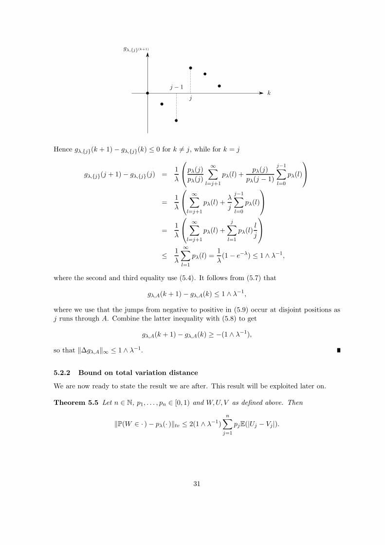
Hence gλ,j(k + 1)− gλ,j(k) ≤ 0 for k 6= j, while for k = j
gλ,j(j + 1)− gλ,j(j) =1
λ
pλ(j)pλ(j)
∞∑
l=j+1
pλ(l) +pλ(j)
pλ(j − 1)
j−1∑
l=0
pλ(l)
=1
λ
∞∑
l=j+1
pλ(l) +λ
j
j−1∑
l=0
pλ(l)
=1
λ
∞∑
l=j+1
pλ(l) +
j∑
l=1
pλ(l)l
j
≤ 1
λ
∞∑
l=1
pλ(l) =1
λ(1− e−λ) ≤ 1 ∧ λ−1,
where the second and third equality use (5.4). It follows from (5.7) that
gλ,A(k + 1)− gλ,A(k) ≤ 1 ∧ λ−1,
where we use that the jumps from negative to positive in (5.9) occur at disjoint positions asj runs through A. Combine the latter inequality with (5.8) to get
gλ,A(k + 1)− gλ,A(k) ≥ −(1 ∧ λ−1),
so that ‖∆gλ,A‖∞ ≤ 1 ∧ λ−1.
5.2.2 Bound on total variation distance
We are now ready to state the result we are after. This result will be exploited later on.
Theorem 5.5 Let n ∈ N, p1, . . . , pn ∈ [0, 1) and W,U, V as defined above. Then
‖P(W ∈ · )− pλ(· )‖tv ≤ 2(1 ∧ λ−1)
n∑
j=1
pjE(|Uj − Vj|).
31
Proof. Pick any A ⊂ N0 and write
P(W ∈ A)− pλ(A) = E(1A(W )− pλ(A)
)
= E(λgλ,A(W + 1)−Wgλ,A(W )
)
=
n∑
j=1
[pjE(gλ,A(W + 1)
)− E
(Yjgλ,A(W )
)]
=n∑
j=1
pj[E(gλ,A(W + 1)
)− E
(gλ,A(W ) | Yj = 1
)]
=
n∑
j=1
pjE(gλ,A(Uj + 1)− gλ,A(Vj + 1)
),
where the second equality uses (5.5), the third equality uses (5.1), while the fifth equality uses(5.2). Applying (5.5) once more, we get
|P(W ∈ A)− pλ(A)| ≤ (1 ∧ λ−1)
n∑
j=1
pjE(|Uj − Vj |),
and taking the supremum over A we get the claim.
To put Theorem 5.5 to use, we look at a subclass of dependent Y1, . . . , Yn.
Definition 5.6 The above random variables Y1, . . . , Yn are said to be negatively related ifthere exist arrays of random variables
Yj1, . . . , YjnY ′j1, . . . , Y
′jn
j = 1, . . . , n,
such that, for each j with P(Yj = 1) > 0,
(Yj1, . . . , Yjn)D=(Y1, . . . , Yn),
(Y ′j1, . . . , Y
′jn)
D=(Y1, . . . , Yn) | Yj = 1,
Y ′ji ≤ Yji ∀ i 6= j,
while, for each j with P(Yj = 1) = 0, Y ′ji = 0 for j 6= i and Y ′
jj = 1.
What negative relation means is that the condition Yj = 1 has a tendency to force Yi = 0for i 6= j. Thus, negative relation is like negative correlation (although the notion is in factstronger).
An important consequence of negative relation is that there exists a coupling such thatUj ≥ Vj for all j. Indeed, we may pick
Uj =
n∑
i=1
Yji, Vj = −1 +n∑
i=1
Y ′ji,
in which case (5.2) is satisfied and, moreover,
Uj − Vj =∑
i=1,...,ni6=j
(Yji − Y ′ji)︸ ︷︷ ︸
≥0
+(1− Y ′jj)︸ ︷︷ ︸
≥0
+ Yjj︸︷︷︸≥0
≥ 0.
The ordering Uj ≥ Vj has the following important consequence.
32
Theorem 5.7 If Y1, . . . , Yn are negatively related, then
‖P(W ∈ ·)− pλ(·)‖tv ≤ 2(1 ∧ λ−1)[λ−Var(W )].
Proof. The ordering Uj ≥ Vj allows us to compute the sum that appears in the bound inTheorem 5.5:
n∑
j=1
pjE(|Uj − Vj|) =
n∑
j=1
pjE(Uj − Vj)
=n∑
j=1
pjE(W )−n∑
j=1
pjE(W | Yj = 1) +n∑
j=1
pj
= E(W )2 −n∑
j=1
E(YjW ) + λ
= E(W )2 − E(W 2) + λ
= −Var(W ) + λ,
where the second equality uses (5.2).
Remark: The upper bound in Theorem 5.7 only contains the unknown quantity Var(W ). Itturns out that in many examples this quantity can be either computed or estimated.
5.3 Two applications
1. Let Y1, . . . , Yn be independent (as assumed previously). Then Var(W ) =∑n
i=1Var(Yi) =∑ni=1 pi(1− pi) = λ−∑n
i=1 p2i , and the bound in Theorem 5.7 reads
2(1 ∧ λ−1)
n∑
i=1
p2i ,
which is better than the bound derived in Section 1.3 when λ ≥ 1.
2. Consider N ≥ 2 urns and 1 ≤ m < N balls. Each urn can contain at most one ball. Placethe balls “randomly” into the urns, i.e., each of the
(Nm
)configurations has equal probability.
For i = 1, . . . , N , letYi = 1urn i contains a ball.
Pick n < N and let W =∑n
i=1 Yi. Then the probability distribution of W is hypergeometric,i.e.,
P(W = k) =
(n
k
)(N − nm− k
)(N
m
)−1
, k = 0 ∨ (m+ n−N), . . . ,m ∧ n,
where(nk
)is the number of ways to place k balls in urns 1, . . . , n and
(N−nm−k
)in the number of
ways to place m− k balls in urns n+ 1, . . . , N .
Exercise 5.8 Check that the right-hand side is a probability distribution. Show that
E(W ) = nmN = λ,
Var(W ) = nmN (1− m
N )N−nN−1 .
33
It is intuitively clear that Y1, . . . , Yn are negatively related: if we condition on urn j tocontain a ball, then urn i with i 6= j is less likely to contain a ball. More formally, recallDefinition 5.6 and, for j = 1, . . . , n, define Yj1, . . . , Yjn and Y ′
j1, . . . , Y′jn as follows:
• Place a ball in urn j.• Place the remaining m− 1 balls randomly in the other N − 1 urns.• Put Y ′
ji = 1urn i contains a ball.• Toss a coin that produces head with probability m
N .• If head comes up, then put (Yj1, . . . , Yjn) = (Y ′
j1, . . . , Y′jn).
• If tail comes up, then pick the ball in urn j, place it randomly in one of the N −m − 1urns that are empty, and put Yji = 1urn i contains a ball.
Exercise 5.9 Check that the above construction produces arrays with the properties requiredby Definition 5.6.
We expect that if m/N,n/N ≪ 1, then W is approximately Poisson distributed. Theformal computation goes as follows. Using Theorem 5.7 and Exercise 5.9, we get
‖P(W ∈ · )− pλ(·)‖tv ≤ 2(1 ∧ λ−1)[λ−Var(W )]
= 2(1 ∧ λ−1)λ
[1−
(1− m
N
) N − nN − 1
]
= 2(1 ∧ λ−1)λ(m+ n− 1)N −mn
N(N − 1)
≤ 2m+ n− 1
N − 1.
Indeed, this is small when m/N,n/N ≪ 1.
34
6 Markov Chains
In Section 1.1 we already briefly described coupling for Markov chains. We now return to thistopic. We recall that X = (Xn)n∈N0
is a Markov chain on a countable state space S, with aninitial distribution λ = (λi)i∈S and with a transition matrix P = (Pij)i,j∈S that is irreducibleand aperiodic.
There are three cases, which will be treated in Sections 6.1–6.3:1. positive recurrent,2. null recurrent,3. transient.
In case 1 there exists a unique stationary distribution π, solving the equation π = πP andsatisfying π > 0, such that limn→∞ λPn = π componentwise on S. The latter is the standardMarkov Chain Convergence Theorem, and we want to investigate the rate of convergence. Incases 2 and 3 there is no stationary distribution, and limn→∞ λPn = 0 componentwise. Wewant to investigate the rate of convergence as well, and see what the role is of the initialdistribution λ.
In Section 6.4 we take a brief look at “perfect simulation”, where coupling of Markov chainsis used to simulate random variables with no error.
6.1 Case 1: Positive recurrent
For i ∈ S, letTi = minn ∈ N : Xn = i,mi = Ei(Ti) = E(Ti | X0 = i),
which, by positive recurrence, are finite. A basic result of Markov chain theory is that πi =1/mi, i ∈ S (see Haggstrom [5], Chapter 5, and Kraaikamp [7], Section 2.2).
We want to compare two copies of the Markov chain starting from different initial distri-butions λ = (λi)i∈S and µ = (µi)i∈S , which we denote by X = (Xn)n∈N0
and X ′ = (X ′n)n∈N0
,respectively. Let
T = minn ∈ N0 : Xn = X ′n
denote their first meeting time. Then the standard coupling inequality in Theorem 2.7 gives
‖λPn − µPn‖tv ≤ 2Pλ,µ(T > n),
where Pλ,µ denotes any probability measure that couples X and X ′. We will choose the
independent coupling Pλ,µ = Pλ ⊗ Pµ, and instead of T focus on
T ∗ = minn ∈ N0 : Xn = X ′n = ∗,
their first meeting time at ∗ (where ∗ is any chosen state in S). Since T ∗ ≥ T , we have
‖λPn − µPn‖tv ≤ 2Pλ,µ(T∗ > n). (6.1)
The key fact that we will uses is the following.
Theorem 6.1 Under positive recurrence,
Pλ,µ(T∗ <∞) = 1 ∀λ, µ.
35
Proof. The successive visits to ∗ by X and X ′, given by the 0, 1-valued random sequences
Y = (Yk)k∈N0with Yk = 1Xk=∗,
Y ′ = (Y ′k)k∈N0
with Y ′k = 1X′
k=∗,
constitute a renewal process: each time ∗ is hit the process of returns to ∗ starts from scratch.Define
Yk = YkY′k, k ∈ N0.
Then also Y = (Yk)k∈N0is a renewal process. Let
I = Yk = 1 for infinitely many k.
It suffices to show that Pλ,µ(I) = 1 for all λ, µ.
If λ = µ = π, then Y is stationary and, since Pπ,π(Y0 = 1) = π20 > 0, it follows from the
renewal property that Pπ,π(I) = 1. Since π > 0, the latter in turn implies that
Pλ,µ(I) = 1,
which yields the claim.
Exercise 6.2 Check the last statement in the proof.
Theorem 6.1 combined with (6.1) implies that
limn→∞
‖λPn − µPn‖tv = 0,
and by picking µ = π we get the Markov Chain Convergence Theorem.
Remark: If |S| <∞, then the convergence is exponentially fast. Indeed, pick k so large that
mini,j∈S
(P k)ijdef= ρ > 0,
which is possible by irreducibility and aperiodicity. Then
Pλ,µ(Xk 6= X ′k) ≤ 1− ρ ∀λ, µ,
and hence, by the Markov property,
Pλ,µ(T > n) ≤ (1− ρ)⌊n/k⌋ ∀λ, µ, n,
where ⌊·⌋ denotes the lower integer part. Via the standard coupling inequality this shows that
‖λPn − µPn‖tv ≤ 2(1− ρ)⌊n/k⌋ = exp[−cn+ o(n)],
with c = 1k log[1/(1 − ρ)] > 0.
Remark: All rates of decay are possible when |S| = ∞: sometimes exponential, sometimespolynomial. With the help of Theorem 2.10 it is possible to estimate the rate when someadditional control on the moments of T or T ∗ is available (recall Section 2.3). This typicallyrequires additional structure. For simple random walk on Z and Z2 it is known that P(T >n) ≍ 1/
√n, respectively, P(T ∗ > n) ≍ 1/ log n (Spitzer [14], Section 3).
36
6.2 Case 2: Null recurrent
Null recurrent Markov chains do not have a stationary distribution. Consequently,
limn→∞
λPn = 0 pointwise ∀λ. (6.2)
Is it still the case thatlimn→∞
‖λPn − µPn‖tv = 0 ∀λ, µ? (6.3)
It suffices to show that there exists a coupling Pλ,µ such that Pλ,µ(T∗ < ∞) = 1. The proof
of Theorem 6.1 for positive recurrent Markov chains does not carry over because there is nostationary distribution. However, it is enough to show that there exists a coupling Pλ,µ such
that Pλ,µ(T < ∞) = 1, which seems easier because the two copies of the Markov chain onlyneed to meet somewhere, not necessarily at ∗.
Theorem 6.3 Under null recurrence,
Pλ,µ(T <∞) = 1 ∀λ, µ.
Proof. A proof of this theorem and hence of (6.3) is beyond the scope of the present course.We refer to Lindvall [11], Section III.21, for more details. As a weak substitute we prove the“Cesaro average” version of (6.3):
X recurrent =⇒ limN→∞
∥∥∥∥∥1
N
N−1∑
n=0
λPn − 1
N
N−1∑
n=0
µPn
∥∥∥∥∥tv
= 0 ∀λ, µ.
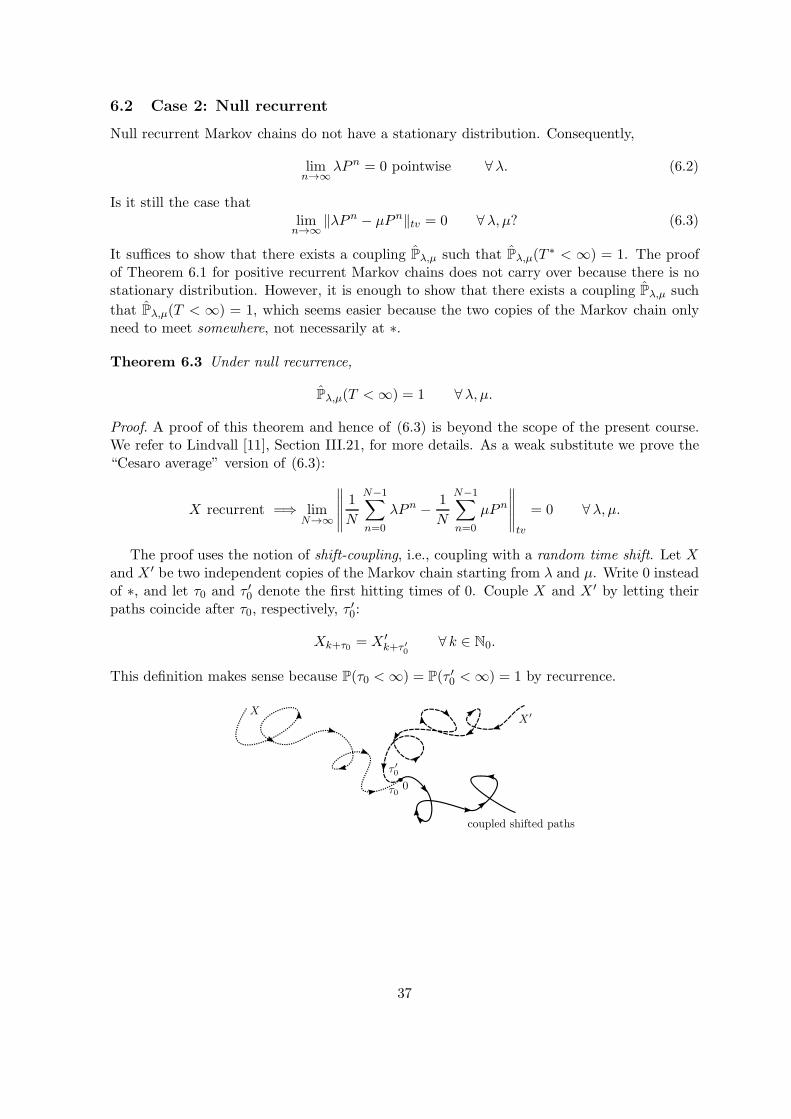
The proof uses the notion of shift-coupling, i.e., coupling with a random time shift. Let Xand X ′ be two independent copies of the Markov chain starting from λ and µ. Write 0 insteadof ∗, and let τ0 and τ ′0 denote the first hitting times of 0. Couple X and X ′ by letting theirpaths coincide after τ0, respectively, τ
′0:
Xk+τ0 = X ′k+τ ′0
∀ k ∈ N0.
This definition makes sense because P(τ0 <∞) = P(τ ′0 <∞) = 1 by recurrence.
37
Fix any event A. Write
∣∣∣∣∣1
N
N−1∑
n=0
(λPn)(A)− 1
N
N−1∑
n=0
(µPn)(A)
∣∣∣∣∣
=1
N
∣∣∣∣∣
N−1∑
n=0
Pλ,µ(Xn ∈ A)−N−1∑
n=0
Pλ,µ(X′n ∈ A)
∣∣∣∣∣
=1
N
∑
m,m′∈N0
Pλ,µ
((τ0, τ
′0) = (m,m′)
)
×∣∣∣∣∣
N−1∑
n=0
Pλ,µ
(Xn ∈ A | (τ0, τ ′0) = (m,m′)
)−
N−1∑
n=0
Pλµ
(X ′
n ∈ A | (τ0, τ ′0) = (m,m′))∣∣∣∣∣
≤ Pλ,µ(τ0 ∨ τ ′0 ≥M) +1
N
∑
m,m′∈N0m∨m′<M
Pλ,µ
((τ0, τ
′0) = (m,m′)
)
×2(m ∨m′) +
∣∣∣∣∣
(N−m−1)∧(N−m′−1)∑
k=0
[Pλ,µ
(Xm+k ∈ A | (τ0, τ ′0) = (m,m′)
)− Pλ,µ
(X ′
m′+k ∈ A | (τ0, τ ′0) = (m,m′))]∣∣∣∣∣
≤ Pλ,µ(τ0 ∨ τ ′0 ≥M) +2
NE((τ0 ∨ τ ′0)1τ0∨τ ′0<M
).
In the first inequality we take M ≤ N and note that m+m′ + |m−m′| = 2(m ∨m′) is thenumber of summands that are lost by letting the sums start at n = m, respectively, n = m′,shifting them bym, respectively, m′, and afterwards cutting them at (N−m−1)∧(N−m′−1).In the second inequality the sum over k is zero by the shift-coupling.
Since the bound is uniform in A, we get the claim by taking the supremum over A andletting N →∞ followed by M →∞.
6.3 Case 3: Transient
There is no general result for transient Markov chains: (6.2) always holds, but (6.3) may holdor may fail. For the special case of random walks on Zd, d ≥ 1, we saw with the help of theOrnstein coupling that (6.3) holds. We also mentioned that for arbitrary random walk
Pλ,µ(T > n) = O(1/√n),
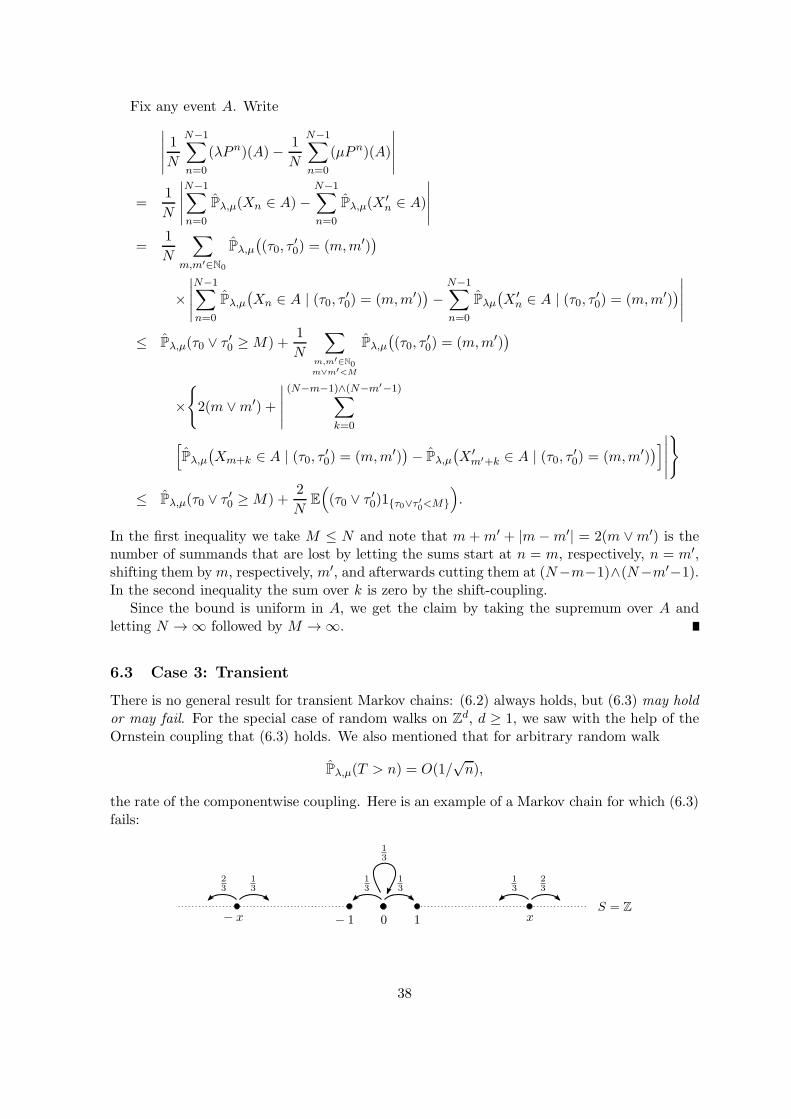
the rate of the componentwise coupling. Here is an example of a Markov chain for which (6.3)fails:
38
At site x the random walk has:
zero drift with pausing for x = 0,positive drift for x > 0,negative drift for x < 0.
This Markov chain is irreducible and aperiodic, with limx→∞ Px(τ0 =∞) = limx→−∞ Px(τ0 =∞) = 1. As a result, we have
limx→∞
lim infn→∞
‖δxPn − δ−xPn‖tv = 2.
6.4 Perfect simulation
The results in Section 6.1 are important for simulation. Suppose that we are given a finite setS, and a probability distribution ρ on S from which we want to draw random samples. Thenwe can proceed as follows. Construct an irreducible and aperiodic Markov chain on S whosestationary distribution is ρ. The Markov Chain Convergence Theorem tells us that if we startthis Markov chain at any site i∗ ∈ S, then after a long time its distribution will be close to ρ.Thus, any late observation of the Markov chain provides us with a good approximation of arandom draw from ρ.
The above approach needs two ingredients:
1. A way to find a transition matrix P on S whose stationary distribution π is equal tothe given probability distribution ρ.
2. A rate of convergence estimate that provides an upper bound on the total variationdistance n 7→ ‖δi∗Pn − π‖tv for a given i∗ ∈ S, so that any desired accuracy of theapproximation can be achieved by running the Markov chain long enough.
Both these ingredients give rise to a theory of simulation, for which an extensive literatureexists (see e.g. Levin, Peres and Williams [8]).
The drawback is that the simulation is at best approximate: no matter how long we runthe Markov chain, its distribution is never perfectly equal to ρ (at least in typical situations).Haggstrom [5], Chapters 10–12, contain an outline of a different approach, through which itis possible to achieve a perfect simulation, i.e., to obtain a random sample whose distributionis equal to ρ with no error (!) In this approach, independent copies of the Markov chain arestarted from each site of S “far back in the past”, and the simulation is stopped at time zerowhen all the copies “have collided prior to time zero”. The observation of the Markov chainat time zero provides the perfect sample.
The details of the construction are somewhat delicate and we refer the reader to the relevantliterature. Concrete examples are discussed in [5].
39
7 Probabilistic inequalities
In Chapters 1 and 3–6 we have seen coupling at work in a number of different situations. Wenow return to the basic theory that was started in Chapter 2. Like the latter, the presentchapter is somewhat technical.
We will show that the existence of an ordered coupling between random variables or ran-dom processes is equivalent to the respective probability measures being ordered themselves.In Sections 7.1 we look at fully ordered state spaces, in Section 7.2 at partially ordered statespaces. In Section 7.3 we state and derive the Fortuin-Kasteleyn-Ginibre inequality, in Sec-tion 7.4 the Holley inequality. Both are inequalities for expectations of functions on partiallyordered state spaces.
7.1 Fully ordered state spaces
Let P,P′ be two probability measures on R such that
P([x,∞)) ≤ P′([x,∞)) ∀x ∈ R,
We say that P′ stochastically dominates P, and write P P′. In terms of the respective cumu-lative distribution functions F,F ′, defined by F (x) = P((−∞, x]) and F ′(x) = P′((−∞, x]),x ∈ R, this property is the same as
F ′(x) ≤ F (x) ∀x ∈ R,
i.e., F ′ ≤ F pointwise.
Theorem 7.1 Let X,X ′ be R-valued random variables with probability measures P,P′. IfP P′, then there exists a coupling (X, X ′) of X and X ′ with probability measure P such that
P(X ≤ X ′) = 1.
Proof. The proof provides an explicit coupling of X and X ′. Let F ∗, F ′∗ denote the generalizedinverse of F,F ′ defined by
F ∗(u) = infx ∈ R : F (x) ≥ u,F ′∗(u) = infx ∈ R : F ′(x) ≥ u, u ∈ (0, 1).
Let U = UNIF(0, 1), and put
X = F ∗(U), X ′ = F ′∗(U).
Then XD=X, X ′ D=X ′, and X ≤ X ′ because F ′ ≤ F implies F ∗ ≤ F ′∗. This construction, via
a common U , provides the desired coupling.
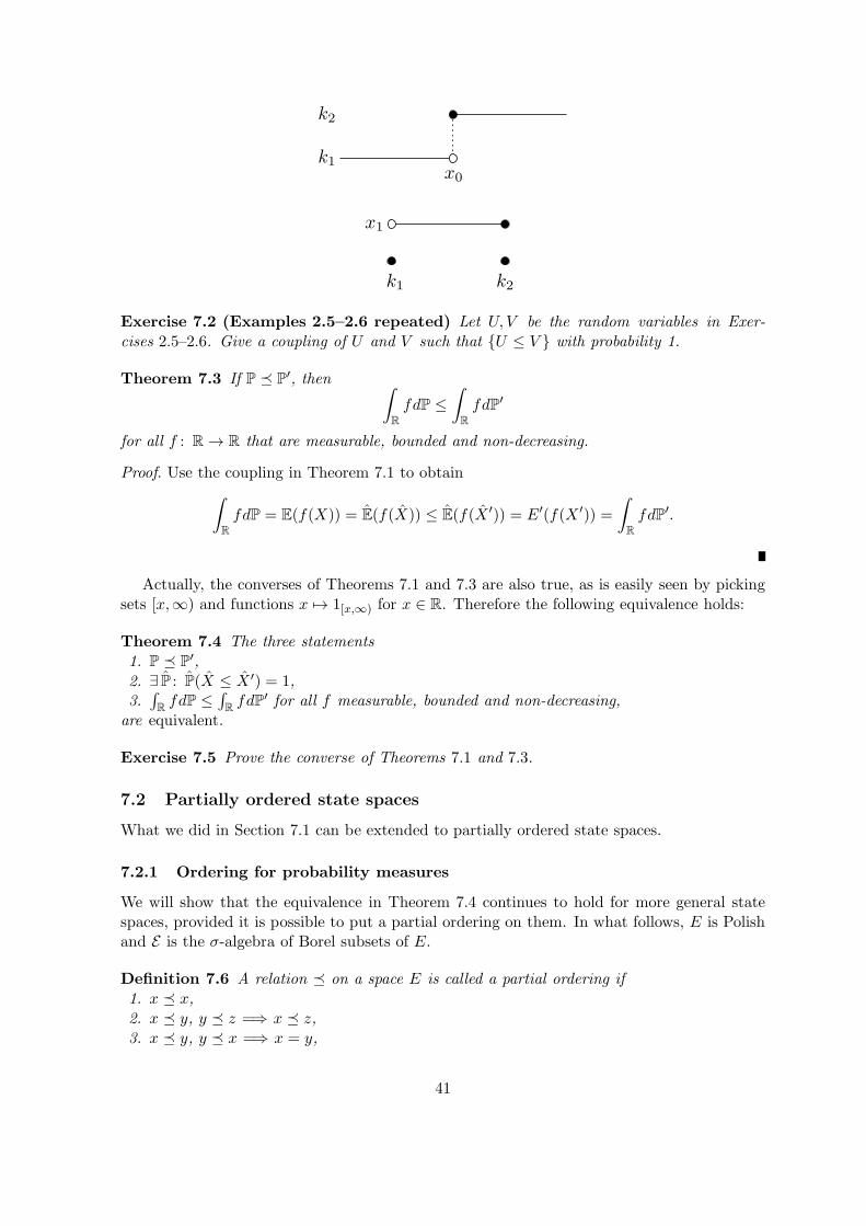
If F has a point mass (k2 − k1)δx0for some k2 > k1 and x0 ∈ R, then this pointmass gives
rise to a flat piece in F ∗ over the interval (k1, k2] at height x1 that solves F (x1) = k2.
40
Exercise 7.2 (Examples 2.5–2.6 repeated) Let U, V be the random variables in Exer-cises 2.5–2.6. Give a coupling of U and V such that U ≤ V with probability 1.
Theorem 7.3 If P P′, then ∫
R
fdP ≤∫
R
fdP′
for all f : R→ R that are measurable, bounded and non-decreasing.
Proof. Use the coupling in Theorem 7.1 to obtain
∫
R
fdP = E(f(X)) = E(f(X)) ≤ E(f(X ′)) = E′(f(X ′)) =∫
R
fdP′.
Actually, the converses of Theorems 7.1 and 7.3 are also true, as is easily seen by pickingsets [x,∞) and functions x 7→ 1[x,∞) for x ∈ R. Therefore the following equivalence holds:
Theorem 7.4 The three statements1. P P′,2. ∃ P : P(X ≤ X ′) = 1,3.∫RfdP ≤
∫RfdP′ for all f measurable, bounded and non-decreasing,
are equivalent.
Exercise 7.5 Prove the converse of Theorems 7.1 and 7.3.
7.2 Partially ordered state spaces
What we did in Section 7.1 can be extended to partially ordered state spaces.
7.2.1 Ordering for probability measures
We will show that the equivalence in Theorem 7.4 continues to hold for more general statespaces, provided it is possible to put a partial ordering on them. In what follows, E is Polishand E is the σ-algebra of Borel subsets of E.
Definition 7.6 A relation on a space E is called a partial ordering if1. x x,2. x y, y z =⇒ x z,3. x y, y x =⇒ x = y,
41
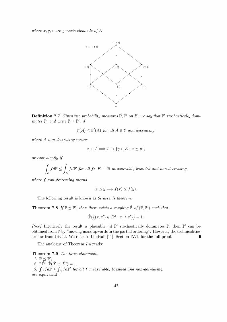
where x, y, z are generic elements of E.
Definition 7.7 Given two probability measures P,P′ on E, we say that P′ stochastically dom-inates P, and write P P′, if
P(A) ≤ P′(A) for all A ∈ E non-decreasing,
where A non-decreasing means
x ∈ A =⇒ A ⊃ y ∈ E : x y,
or equivalently if∫
EfdP ≤
∫
EfdP′ for all f : E → R measureable, bounded and non-decreasing,
where f non-decreasing means
x y =⇒ f(x) ≤ f(y).
The following result is known as Strassen’s theorem.
Theorem 7.8 If P P′, then there exists a coupling P of (P,P′) such that
P((x, x′) ∈ E2 : x x′
)= 1.
Proof. Intuitively the result is plausible: if P′ stochastically dominates P, then P′ can beobtained from P by “moving mass upwards in the partial ordering”. However, the technicalitiesare far from trivial. We refer to Lindvall [11], Section IV.1, for the full proof.
The analogue of Theorem 7.4 reads:
Theorem 7.9 The three statements1. P P′,2. ∃ P : P(X X ′) = 1,3.∫E fdP ≤
∫E fdP
′ for all f measurable, bounded and non-decreasing,are equivalent.
42
Examples:
• E = 0, 1Z, x = (xi)i∈Z ∈ E, x y if and only if xi ≤ yi for all i ∈ Z. For p ∈ [0, 1],let Pp denote the probability measure on E under which X = (Xi)i∈Z has i.i.d. BER(p)components. Then Pp Pp′ if and only if p ≤ p′.
• It is possible to build in dependency. For instance, let Y = (Yi)i∈Z be defined by
Yi = 1Xi−1=Xi=1,
and let Pp be the law of Y induced by the law Pp of X. Then the components of Y are
not independent, but again Pp Pp′ if and only if p ≤ p′.
Exercise 7.10 Prove the last two claims.
More examples will be encountered in Chapter 9.
Exercise 7.11 Does in Definition 7.7 define a partial ordering on the space of probabilitymeasures?
7.2.2 Ordering for Markov chains
The notions of partial ordering and stochastic domination are important also for Markovchains. Let E be a polish space equipped with a partial ordering . A transition kernel Kon E × E is a mapping from E × E to [0, 1] such that:
1. K(x, ·) is a probability measure on E for every x ∈ E;2. K(·, A) is a measurable mapping from E to [0, 1] for every A ∈ E .The meaning of K(x,A) is the probability for the Markov chain to jump from x into A.
An example is
E = Rd, K(x,A) =1
|B1(x)||B1(x) ∩A|,
which corresponds to a “Levy flight” on Rd, i.e., a random walk that makes i.i.d. jumps drawnrandomly from the unit ball B1(0) around the origin. The special case where E is a countableset leads to transition kernels taking the form K(i, A) =
∑j∈A Pij , i ∈ E, for some transition
matrix P = (Pij)i,j∈E.
Definition 7.12 Given two transition kernels K and K ′ on E × E, we say that K ′ stochas-tically dominates K if
K(x, ·) K ′(x′, ·) for all x x′.If K = K ′ and the latter condition holds, then we say that K is monotone.
Remark: Not all transition kernels are monotone, which is why we cannot write K K ′
for the property in Definition 7.12, i.e., there is no partial ordering on the set of transitionkernels.
Lemma 7.13 If λ µ and K ′ stochastically dominates K, then
λKn µK ′n for all n ∈ N0.
43
Proof. The proof is by induction on n. The ordering holds for n = 0. Suppose that theordering holds for n. Let f be an arbitrary bounded and non-decreasing function on En+2.Then ∫
En+2
f(x0, . . . , xn, xn+1)(λKn+1)(dx0, . . . , dxn, dxn+1)
=
∫
En+1
(λKn)(dx0, . . . , dxn)
∫
Ef(x0, . . . , xn, xn+1)K(xn, dxn+1),
(7.1)
where (λKn)(dx0, . . . , dxn) is an abbreviation for λ(dx0)K(x0, dx1) × · · · × K(xn−1, dxn).The last integral is a function of x0, . . . , xn. Since f is non-decreasing and K ′ stochasticallydominates K, this integral is bounded from above by
∫
Ef(x0, . . . , xn, xn+1)K
′(xn, dxn+1), (7.2)
where we use Definitions 7.7 and 7.12.
Exercise 7.14 Check the above computation.
Since the ordering holds for n and (7.2) is a non-decreasing function of (x0, . . . , xn), theright-hand side of (7.1) is bounded from above by
∫
En+1
(µK ′n)(dx0, . . . , dxn)∫
Ef(x0, . . . , xn, xn+1)K
′(xn, dxn+1),
which equals ∫
En+2
f(x0, . . . , xn, xn+1)(µK′n+1)(dx0, . . . , dxn, dxn+1).
This proves the claim by Definition 7.6.
By using the Kolmogorov extension theorem, the result in Lemma 7.13 can be extended ton =∞, i.e., the ordering also holds for infinite sequences. This has the following consequence.
Theorem 7.15 If λ µ and K ′ stochastically dominates K, then there exist E-valued ran-dom processes
Z = (Zn)n∈N0, Z ′ = (Z ′
n)n∈N0,
such that
(Z0, . . . , Zn)D=λKn,
(Z ′0, . . . , Z
′n)
D=µK ′n,
∀n ∈ N0,
and Z0 Z ′0, Z1 Z ′
1, . . . a.s. w.r.t. the joint law of (Z,Z ′).
Remark: The last ordering is denoted by Z ∞ Z ′. All components are ordered w.r.t. .Examples:
1. E = R, becomes ≤. The result says that if λD≤µ and K(x, ·)
D≤K ′(x, ·) for all x ≤ x′,
then the two Markov chains on R can be coupled so that they are ordered for all times.2. E = 0, 1Z. Think of an infinite sequence of lamps, labelled by Z, that can be either
“off” or “on”. The initial distributions are λ = Pp and µ = Pp′ with p < p′. The transitionkernels K and K ′ are such that the lamps change their state independently at rates
K : 0u−→1, 1
v−→0,
K ′ : 0u′
−→1, 1v′−→0,
with u′ > u and v′ < v, i.e., K ′ flips more rapidly on and less rapidly off compared to K.
44
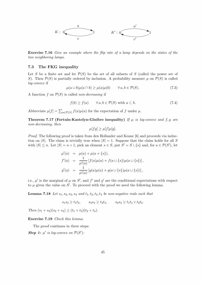
Exercise 7.16 Give an example where the flip rate of a lamp depends on the states of thetwo neighboring lamps.
7.3 The FKG inequality
Let S be a finite set and let P(S) be the set of all subsets of S (called the power set ofS). Then P(S) is partially ordered by inclusion. A probability measure µ on P(S) is calledlog-convex if
µ(a ∪ b)µ(a ∩ b) ≥ µ(a)µ(b) ∀ a, b ∈ P(S). (7.3)
A function f on P(S) is called non-decreasing if
f(b) ≥ f(a) ∀ a, b ∈ P(S) with a ⊂ b. (7.4)
Abbreviate µ[f ] =∑
a∈P(S) f(a)µ(a) for the expectation of f under µ.
Theorem 7.17 (Fortuin-Kastelyn-Ginibre inequality) If µ is log-convex and f, g arenon-decreasing, then
µ[fg] ≥ µ[f ]µ[g].
Proof. The following proof is taken from den Hollander and Keane [6] and proceeds via induc-tion on |S|. The claim is trivially true when |S| = 1. Suppose that the claim holds for all Swith |S| ≤ n. Let |S| = n+ 1, pick an element s ∈ S, put S′ = S \ s and, for a ∈ P(S′), let
µ′(a) = µ(a) + µ(a+ s),
f ′(a) =1
µ′(a)[f(a)µ(a) + f(a ∪ s)µ(a ∪ s)] ,
g′(a) =1
µ′(a)[g(a)µ(a) + g(a ∪ s)µ(a ∪ s)] ,
i.e., µ′ is the marginal of µ on S′, and f ′ and g′ are the conditional expectations with respectto µ given the value on S′. To proceed with the proof we need the following lemma.
Lemma 7.18 Let s1, s2, s3, s4 and t1, t2, t3, t4 be non-negative reals such that
s1s2 ≥ t1t2, s3s4 ≥ t3t4, s2s3 ≥ t1t4 ∨ t2t3.
Then (s1 + s3)(s2 + s4) ≥ (t1 + t3)(t2 + t4).
Exercise 7.19 Check this lemma.
The proof continues in three steps:
Step 1: µ′ is log-convex on P(S′):
45
Use (7.3) and Lemma 7.18 with a, b ∈ P(S′) and
s1 = µ(a ∪ b) t1 = µ(a)s2 = µ(a ∩ b) t2 = µ(b)s3 = µ([a ∪ b] ∪ s) t3 = µ(a ∪ s)s4 = µ([a ∩ b] ∪ s) t4 = µ(b ∪ s)
to obtain µ′(a ∪ b)µ′(a ∩ b) ≥ µ′(a)µ′(b).
Exercise 7.20 Check the latter inequality.
Step 2: f ′, g′ are non-decreasing on P(S′):
For a, b ∈ P(S′) with a ⊂ b, write
f ′(b)− f ′(a) = 1
µ′(a)µ′(b)
[µ(a) + µ(a ∪ s)][f(b)µ(b) + f(b ∪ s)µ(b ∪ s)]
− [µ(b) + µ(b ∪ s)][f(a)µ(a) + f(a ∪ s)µ(a ∪ s)]
=1
µ′(a)µ′(b)[µ(a) + µ(a ∪ s)]
×[f(b)− f(a)]︸ ︷︷ ︸
≥0
µ(b) + [f(b ∪ s)− f(a ∪ s)]︸ ︷︷ ︸≥0
µ(b ∪ s)
+ [f(a ∪ s)− f(a)]︸ ︷︷ ︸≥0
[µ(a)µ(b ∪ s)− µ(a ∪ s)µ(b)]︸ ︷︷ ︸≥0
≥ 0.
The right-hand side is a sum of products of non-negative terms (use (7.3–7.4)), and so f ′(b) ≥f ′(a).
Step 3: µ[fg] ≥ µ′[f ′g′]:Write
µ[fg] =∑
a∈P(S)
(fg)(a)µ(a) =∑
a∈P(S′)
(fg)′(a)µ′(a),
and use that
µ′(a)2[(fg)′(a)− f ′(a)g′(a)
]
= [µ(a) + µ(a ∪ s)] [(fg)(a)µ(a) + (fg)(a ∪ s)µ(a ∪ s)]− [f(a)µ(a) + f(a ∪ s)µ(a ∪ s)] [g(a)µ(a) + g(a ∪ s)µ(a ∪ s)]
= µ(a)µ(a ∪ s) [f(a ∪ s)− f(a)]︸ ︷︷ ︸≥0
[g(a ∪ s)− g(a)]︸ ︷︷ ︸≥0
≥ 0.
Henceµ[fg] ≥
∑
a∈P(S)
f ′(a)g′(a)µ′(a).
By the induction assumption in combination with Steps 1 and 2, we have
µ′[f ′g′] ≥ µ′[f ′]µ′[g′].
But µ′[f ′] = µ[f ] and µ′[g′] = µ[g], and so with Step 3 we are done when µ > 0 on P(S).
46
Exercise 7.21 Explain how to remove the restriction that µ > 0 on P(S).
Remark: By taking a “projective limit” |S| → ∞, it is trivial to extend Theorem 7.17 tocountable sets S. The inequality in (7.3) must then be assumed for arbitrary cylinder sets. Itis even possible to extend to uncountable sets S.
Remark: The condition of log-convexity of µ is not necessary on fully ordered spaces. Indeed,pick S = R, let f, g be any two non-decreasing functions on R, and write
µ[fg]− µ[f ]µ[g] =∫
R
µ(dx) f(x)g(x) −∫
R
µ(dx) f(x)
∫
R
µ(dy) g(y)
= 12
∫
R
µ(dx)
∫
R
µ(dy) [f(x)− f(y)][g(x) − g(y)]︸ ︷︷ ︸≥0
≥ 0.
The two factors in the integrand are either both ≥ 0 or both ≤ 0, and hence µ[fg] ≥ µ[f ]µ[g].Remark: The intuition behind log-convexity is the following. First, note that the inequalityin (7.3) holds for all a, b ∈ P(S) if and only if
µ(a ∪ s)µ(a)
≥ µ(s)µ(∅) ∀ a ∈ P(S), s ∈ S\a. (7.5)
Next, let X ∈ P(S) be the random variable with distribution P(X = a) = µ(a), a ∈ P(S).Define
p(a, s) = P(s ∈ X | X ∩ S\s = a
), ∀ a ∈ P(S), s ∈ S\a, (7.6)
and note that
p(a, s) =(1 +
(µ(a ∪ s)µ(a)
)−1)−1
.
Therefore (7.5) is the same as
p(a, s) ≥ p(∅, s) a ∈ P(S), s ∈ S\a.
In view of (7.6), the latter says: “larger X are more likely to contain an extra point thansmaller X”, a property referred to as “attractiveness”.
Example: [Percolation model]Take S to be a finite set in Zd, P(S) = 0, 1S ,
µ(a) = p|a|(1− p)|S\a| with p ∈ (0, 1), (7.7)
A,B ⊂ S and f(·) = 1·⊃A, g(·) = 1·⊃B. Then
µ(all 1′s on A ∪B) ≥ µ(all 1′s on A)µ(all 1′s on B). (7.8)
Exercise 7.22 Prove (7.8) by checking that µ is log-convex.
Under the probability distribution in (7.7), each site in S carries a particle (= 1) with prob-ability p or a vacancy (= 0) with probability 1 − p, independently for different sites. This isreferred to as percolation and will be treated in more detail in Chapter 8.
47

Example: [Ising model]Take S to be a finite torus in Zd (with periodic boundary conditions), P(S) = 0, 1S ,
µ(a) = 1Zβ
exp[β|x, y ∈ a : ‖x− y‖ = 1|
]with β ∈ (0,∞),
where Zβ is the normalizing constant,(7.9)
A,B ⊂ S and f(·) = 1·⊃A, g(·) = 1·⊃B.
Exercise 7.23 Prove (7.8) by checking that µ is log-convex.
The probability distribution in (7.9) gives a probabilistic reward eβ to every pair of 1’s in Sthat are located at nearest-neighbor sites. It is used in statistical physics to describe a systemconsisting of particles that have a tendency to stick to each other when they are close to eachother, due to the so-called van der Waals force (1 = particle, 0 = vacancy). The parameterβ plays the role of the “inverse temperature”: the lower the temperature, the larger β, andhence the larger the tendency to stick to each other. This is referred to as ferromagnetismand will be treated in more detail in Chapter 9.
7.4 The Holley inequality
A variant of the FKG-inequality is the following. Given two probability measures µ1, µ2 onP(S), we say that µ1 is log-convex with respect to µ2 if
µ1(a ∪ b)µ2(a ∩ b) ≥ µ1(a)µ2(b) ∀ a, b ∈ P(S). (7.10)
Note that a probability measure µ on P(S) is log-convex with respect to itself if and only itis log-convex in the sense of (7.3).
Theorem 7.24 If µ1 is log-convex with respect to µ2 and f is non-decreasing, then
µ1[f ] ≥ µ2[f ].Proof. See den Hollander and Keane [6] for a proof similar to that of Theorem 7.17. Here wegive a proof that uses Lemma 7.13. Again we assume that µ1, µ2 > 0 on P(S), a restrictionthat is easily removed afterwards.
We construct a coupling of two continuous-time Markov chains
η = (ηt)t≥0, ζ = (ζt)t≥0,
on P(S), with S finite, such that:
(1) η has stationary distribution µ2,(2) ζ has stationary distribution µ1,(3) the coupling prevents the pair (η, ζ) to exit the set (a, b) ∈ P(S)2 : a ⊂ b.
The rates of the coupled Markov chain are chosen as follows. For s ∈ S, let ηs denotethe element of P(S) = 0, 1S obtained from η by flipping the variable at s (either 0 → 1 or1→ 0). Allow only the following transitions:
(η, ζ)→ (ηs, ζ) at rate
1 if (η(s), ζ(s)) = (0, 1),µ2(ηs)µ2(η)
− µ1(ζs)µ1(ζ)
if (η(s), ζ(s)) = (1, 1),
(η, ζ)→ (η, ζs) at rate µ1(ζs)µ1(ζ)
if (η(s), ζ(s)) = (0, 1),
(η, ζ)→ (ηs, ζs) at rate
1 if (η(s), ζ(s)) = (0, 0),µ1(ζs)µ1(ζ)
if (η(s), ζ(s)) = (1, 1).
48
Exercise 7.25 Check property (3) by showing that the allowed transitions preserve the order-ing of the Markov chains, i.e., if η ⊆ ζ, then the same is true after every allowed transition.Consequently,
η0 ⊆ ζ0 =⇒ ηt ⊆ ζt ∀ t > 0. (7.11)
Check properties (1) and (2). Condition (7.10) is needed to ensure that
µ2(ηs)
µ2(η)≥ µ1(ζ
s)
µ1(ζ)when η ⊆ ζ with (η(s), ζ(s)) = (1, 1).
From (7.11) we get Eη0(f(ηt)) ≤ Eζ0(f(ζt)) for all t ≥ 0 when η0 ⊂ ζ0, and the Holleyinequality follows because Eη0(f(ηt))→ µ2[f ] and Eζ0(f(ζt))→ µ1[f ] as t→∞. Pick η0 = ∅and ζ0 = S to make sure that η0 ⊆ ζ0.
Remark: The coupling used in the above proof is a maximal coupling in the sense of Sec-tion 2.5.
Remark: By viewing the above rates locally, we can extend the Holley inequality to countablesets S via a “projective limit” argument. The inequality in (7.10) must then be assumed forarbitrary cylinder sets. It is even possible to extend to uncountable sets S.
What is important about Theorem 7.24 is that it provides an explicit criterion on µ1, µ2such that µ2 µ1, as is evident from Theorem 7.9. Note that “log-convex with respect to” isnot a partial ordering: as noted above, µ is log-convex with respect to itself if and only if itis log-convex. In particular, the reverse of Theorem 7.24 is false.
Exercise 7.26 Return to the example of the Ising model at the end of Section 7.3. Pickβ1 > β2, and let µi = µβi
, i = 1, 2, with µβ the probability measure in (7.9). Show that µβ1is
log-convex with respect to µβ2.
Remark: FKG follows from Holley by choosing
µ1 =µg
µ[g], µ2 = µ. (7.12)
Exercise 7.27 Check this claim.
49
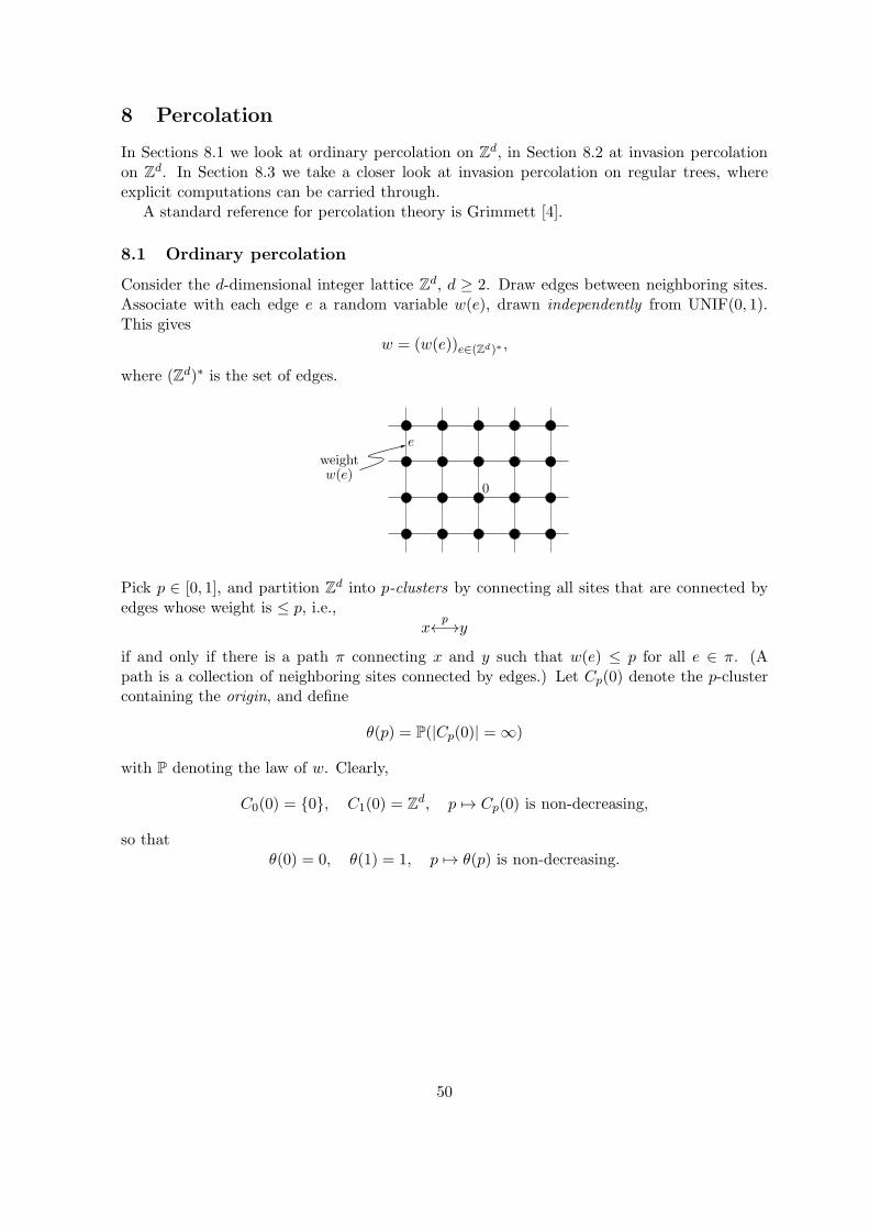
8 Percolation
In Sections 8.1 we look at ordinary percolation on Zd, in Section 8.2 at invasion percolationon Zd. In Section 8.3 we take a closer look at invasion percolation on regular trees, whereexplicit computations can be carried through.
A standard reference for percolation theory is Grimmett [4].
8.1 Ordinary percolation
Consider the d-dimensional integer lattice Zd, d ≥ 2. Draw edges between neighboring sites.Associate with each edge e a random variable w(e), drawn independently from UNIF(0, 1).This gives
w = (w(e))e∈(Zd)∗ ,
where (Zd)∗ is the set of edges.
Pick p ∈ [0, 1], and partition Zd into p-clusters by connecting all sites that are connected byedges whose weight is ≤ p, i.e.,
xp←→y
if and only if there is a path π connecting x and y such that w(e) ≤ p for all e ∈ π. (Apath is a collection of neighboring sites connected by edges.) Let Cp(0) denote the p-clustercontaining the origin, and define
θ(p) = P(|Cp(0)| =∞)
with P denoting the law of w. Clearly,
C0(0) = 0, C1(0) = Zd, p 7→ Cp(0) is non-decreasing,
so thatθ(0) = 0, θ(1) = 1, p 7→ θ(p) is non-decreasing.
50
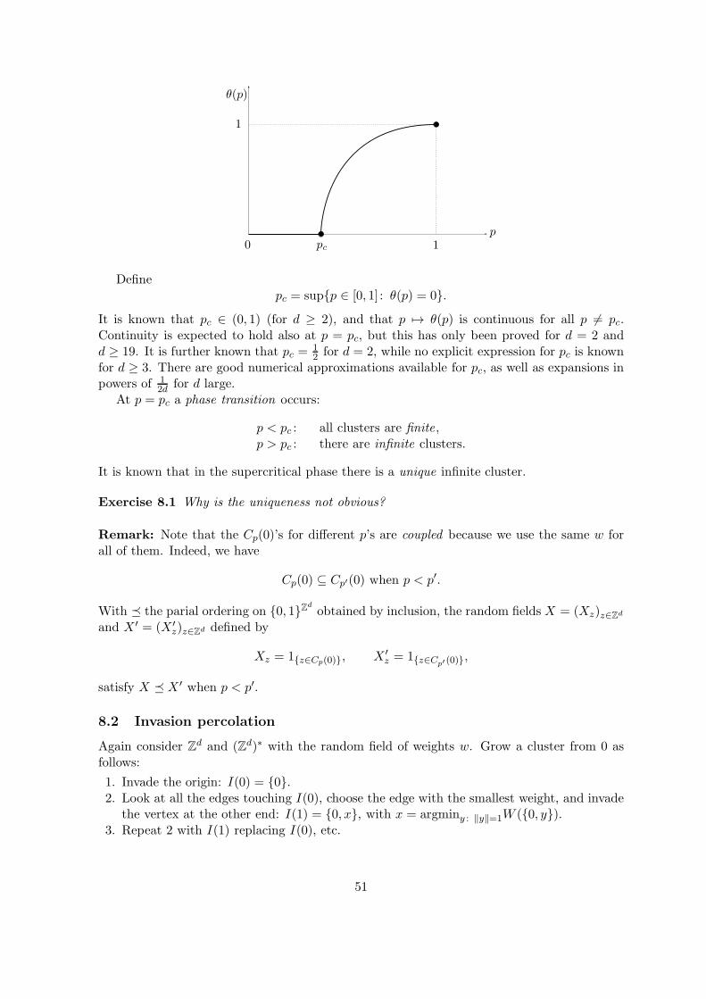
Definepc = supp ∈ [0, 1] : θ(p) = 0.
It is known that pc ∈ (0, 1) (for d ≥ 2), and that p 7→ θ(p) is continuous for all p 6= pc.Continuity is expected to hold also at p = pc, but this has only been proved for d = 2 andd ≥ 19. It is further known that pc =
12 for d = 2, while no explicit expression for pc is known
for d ≥ 3. There are good numerical approximations available for pc, as well as expansions inpowers of 1
2d for d large.At p = pc a phase transition occurs:
p < pc : all clusters are finite,p > pc : there are infinite clusters.
It is known that in the supercritical phase there is a unique infinite cluster.
Exercise 8.1 Why is the uniqueness not obvious?
Remark: Note that the Cp(0)’s for different p’s are coupled because we use the same w forall of them. Indeed, we have
Cp(0) ⊆ Cp′(0) when p < p′.
With the parial ordering on 0, 1Zdobtained by inclusion, the random fields X = (Xz)z∈Zd
and X ′ = (X ′z)z∈Zd defined by
Xz = 1z∈Cp(0), X ′z = 1z∈Cp′ (0),
satisfy X X ′ when p < p′.
8.2 Invasion percolation
Again consider Zd and (Zd)∗ with the random field of weights w. Grow a cluster from 0 asfollows:
1. Invade the origin: I(0) = 0.2. Look at all the edges touching I(0), choose the edge with the smallest weight, and invade
the vertex at the other end: I(1) = 0, x, with x = argminy : ‖y‖=1W (0, y).3. Repeat 2 with I(1) replacing I(0), etc.
51
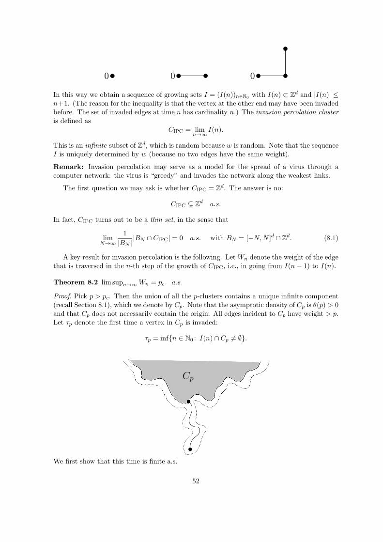
In this way we obtain a sequence of growing sets I = (I(n))n∈N0with I(n) ⊂ Zd and |I(n)| ≤
n+1. (The reason for the inequality is that the vertex at the other end may have been invadedbefore. The set of invaded edges at time n has cardinality n.) The invasion percolation clusteris defined as
CIPC = limn→∞
I(n).
This is an infinite subset of Zd, which is random because w is random. Note that the sequenceI is uniquely determined by w (because no two edges have the same weight).
Remark: Invasion percolation may serve as a model for the spread of a virus through acomputer network: the virus is “greedy” and invades the network along the weakest links.
The first question we may ask is whether CIPC = Zd. The answer is no:
CIPC ( Zd a.s.
In fact, CIPC turns out to be a thin set, in the sense that
limN→∞
1
|BN ||BN ∩CIPC| = 0 a.s. with BN = [−N,N ]d ∩ Zd. (8.1)
A key result for invasion percolation is the following. LetWn denote the weight of the edgethat is traversed in the n-th step of the growth of CIPC, i.e., in going from I(n − 1) to I(n).
Theorem 8.2 lim supn→∞Wn = pc a.s.
Proof. Pick p > pc. Then the union of all the p-clusters contains a unique infinite component(recall Section 8.1), which we denote by Cp. Note that the asymptotic density of Cp is θ(p) > 0and that Cp does not necessarily contain the origin. All edges incident to Cp have weight > p.Let τp denote the first time a vertex in Cp is invaded:
τp = infn ∈ N0 : I(n) ∩ Cp 6= ∅.
We first show that this time is finite a.s.
52
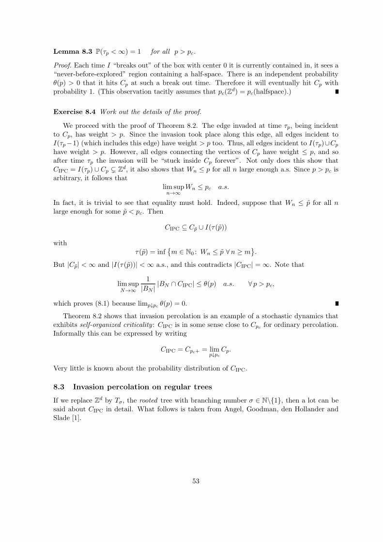
Lemma 8.3 P(τp <∞) = 1 for all p > pc.
Proof. Each time I “breaks out” of the box with center 0 it is currently contained in, it sees a“never-before-explored” region containing a half-space. There is an independent probabilityθ(p) > 0 that it hits Cp at such a break out time. Therefore it will eventually hit Cp withprobability 1. (This observation tacitly assumes that pc(Z
d) = pc(halfspace).)
Exercise 8.4 Work out the details of the proof.
We proceed with the proof of Theorem 8.2. The edge invaded at time τp, being incidentto Cp, has weight > p. Since the invasion took place along this edge, all edges incident toI(τp−1) (which includes this edge) have weight > p too. Thus, all edges incident to I(τp)∪Cp
have weight > p. However, all edges connecting the vertices of Cp have weight ≤ p, and soafter time τp the invasion will be “stuck inside Cp forever”. Not only does this show thatCIPC = I(τp) ∪ Cp ( Zd, it also shows that Wn ≤ p for all n large enough a.s. Since p > pc isarbitrary, it follows that
lim supn→∞
Wn ≤ pc a.s.
In fact, it is trivial to see that equality must hold. Indeed, suppose that Wn ≤ p for all nlarge enough for some p < pc. Then
CIPC ⊆ Cp ∪ I(τ(p))
withτ(p) = inf
m ∈ N0 : Wn ≤ p ∀n ≥ m
.
But |Cp| <∞ and |I(τ(p))| <∞ a.s., and this contradicts |CIPC| =∞. Note that
lim supN→∞
1
|BN ||BN ∩ CIPC| ≤ θ(p) a.s. ∀ p > pc,
which proves (8.1) because limp↓pc θ(p) = 0.
Theorem 8.2 shows that invasion percolation is an example of a stochastic dynamics thatexhibits self-organized criticality : CIPC is in some sense close to Cpc for ordinary percolation.Informally this can be expressed by writing
CIPC = Cpc+ = limp↓pc
Cp.
Very little is known about the probability distribution of CIPC.
8.3 Invasion percolation on regular trees
If we replace Zd by Tσ, the rooted tree with branching number σ ∈ N\1, then a lot can besaid about CIPC in detail. What follows is taken from Angel, Goodman, den Hollander andSlade [1].
53
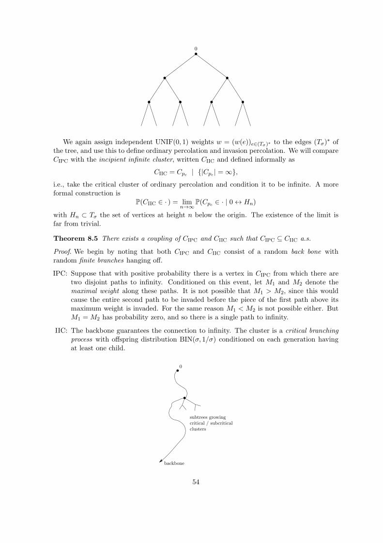
We again assign independent UNIF(0, 1) weights w = (w(e))e∈(Tσ )∗ to the edges (Tσ)∗ of
the tree, and use this to define ordinary percolation and invasion percolation. We will compareCIPC with the incipient infinite cluster, written CIIC and defined informally as
CIIC = Cpc | |Cpc | =∞,i.e., take the critical cluster of ordinary percolation and condition it to be infinite. A moreformal construction is
P(CIIC ∈ · ) = limn→∞
P(Cpc ∈ · | 0↔ Hn)
with Hn ⊂ Tσ the set of vertices at height n below the origin. The existence of the limit isfar from trivial.
Theorem 8.5 There exists a coupling of CIPC and CIIC such that CIPC ⊆ CIIC a.s.
Proof. We begin by noting that both CIPC and CIIC consist of a random back bone withrandom finite branches hanging off.
IPC: Suppose that with positive probability there is a vertex in CIPC from which there aretwo disjoint paths to infinity. Conditioned on this event, let M1 and M2 denote themaximal weight along these paths. It is not possible that M1 > M2, since this wouldcause the entire second path to be invaded before the piece of the first path above itsmaximum weight is invaded. For the same reason M1 < M2 is not possible either. ButM1 =M2 has probability zero, and so there is a single path to infinity.
IIC: The backbone guarantees the connection to infinity. The cluster is a critical branchingprocess with offspring distribution BIN(σ, 1/σ) conditioned on each generation havingat least one child.
54
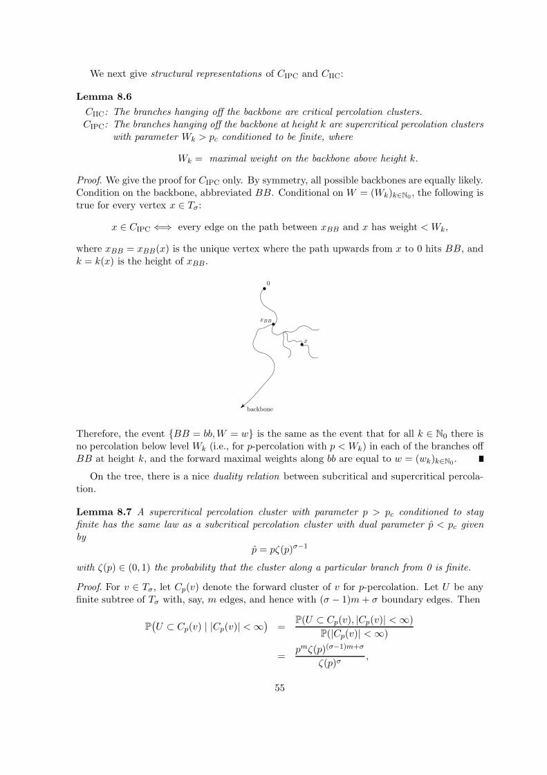
We next give structural representations of CIPC and CIIC:
Lemma 8.6
CIIC: The branches hanging off the backbone are critical percolation clusters.CIPC: The branches hanging off the backbone at height k are supercritical percolation clusters
with parameter Wk > pc conditioned to be finite, where
Wk = maximal weight on the backbone above height k.
Proof. We give the proof for CIPC only. By symmetry, all possible backbones are equally likely.Condition on the backbone, abbreviated BB. Conditional on W = (Wk)k∈N0
, the following istrue for every vertex x ∈ Tσ:
x ∈ CIPC ⇐⇒ every edge on the path between xBB and x has weight < Wk,
where xBB = xBB(x) is the unique vertex where the path upwards from x to 0 hits BB, andk = k(x) is the height of xBB .
Therefore, the event BB = bb,W = w is the same as the event that for all k ∈ N0 there isno percolation below level Wk (i.e., for p-percolation with p < Wk) in each of the branches offBB at height k, and the forward maximal weights along bb are equal to w = (wk)k∈N0
.
On the tree, there is a nice duality relation between subcritical and supercritical percola-tion.
Lemma 8.7 A supercritical percolation cluster with parameter p > pc conditioned to stayfinite has the same law as a subcritical percolation cluster with dual parameter p < pc givenby
p = pζ(p)σ−1
with ζ(p) ∈ (0, 1) the probability that the cluster along a particular branch from 0 is finite.
Proof. For v ∈ Tσ, let Cp(v) denote the forward cluster of v for p-percolation. Let U be anyfinite subtree of Tσ with, say, m edges, and hence with (σ − 1)m+ σ boundary edges. Then
P(U ⊂ Cp(v) | |Cp(v)| <∞
)=
P(U ⊂ Cp(v), |Cp(v)| <∞)
P(|Cp(v)| <∞)
=pmζ(p)(σ−1)m+σ
ζ(p)σ,
55
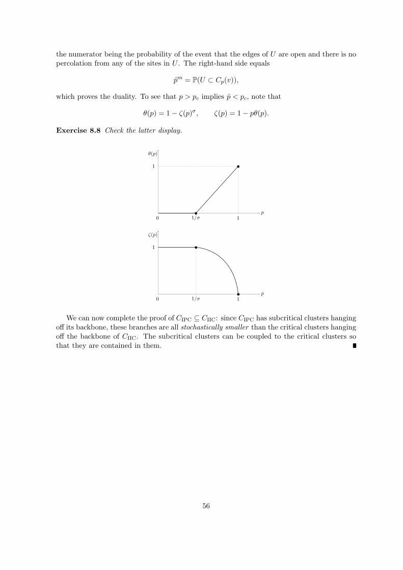
the numerator being the probability of the event that the edges of U are open and there is nopercolation from any of the sites in U . The right-hand side equals
pm = P(U ⊂ Cp(v)),
which proves the duality. To see that p > pc implies p < pc, note that
θ(p) = 1− ζ(p)σ, ζ(p) = 1− pθ(p).
Exercise 8.8 Check the latter display.
We can now complete the proof of CIPC ⊆ CIIC: since CIPC has subcritical clusters hangingoff its backbone, these branches are all stochastically smaller than the critical clusters hangingoff the backbone of CIIC. The subcritical clusters can be coupled to the critical clusters sothat they are contained in them.
56
9 Interacting particle systems
In Section 9.1 we define what an interacting particle system is. In Sections 9.2–9.3 we focus onshift-invariant spin-flip systems, which constitute a particularly tractable class of interactingparticle systems, and look at their convergence to equilibrium. In Section 9.4 we give threeexamples in this class: Stochastic Ising Model, Contact Process, Voter Model. In Section 9.5we take a closer look at the Contact Process.
The standard reference for interacting particle systems is Liggett [9].
9.1 Definitions
An Interacting Particle System (IPS) is a Markov process ξ = (ξt)t≥0 on the state space
Ω = 0, 1Zd(or Ω = −1, 1Zd
), d ≥ 1, where
ξt = ξt(x) : x ∈ Zd
denotes the configuration at time t, with ξt(x) = 1 or 0 meaning that there is a “particle” or“hole” at site x at time t, respectively. Alternative interpretations are
1 = infected/spin-up/democrat0 = healthy/spin-down/republican.
The configuration changes with time and this models how a virus spreads through a popula-tion, how magnetic atoms in iron flip up and down as a result of noise due to temperature, orhow the popularity of two political parties evolves in an election campaign.
The evolution is modeled by specifying a set of local transition rates
c(x, η), x ∈ Zd, η ∈ Ω, (9.1)
playing the role of the rate at which the state at site x changes in the configuration η, i.e.,
η → ηx
with ηx the configuration obtained from η by changing the state at site x (either 0 → 1 or1→ 0). Since there are only two possible states at each site, such systems are called spin-flipsystems.
Remark: It is possible to allow more than two states, e.g. −1, 0, 1 or N0. It is also possibleto allow more than one site to change state at a time, e.g. swapping of states 01 → 10 or10→ 01. In what follows we focus entirely on spin-flip systems.
If c(x, η) depends on η only via η(x), the value of the spin at x, then ξ consists of indepen-dent spin-flips. In general, however, the rate to flip the spin at x may depend on the spins inthe neighborhood of x (possibly even on all spins). This dependence models an “interaction”between the spins at different sites. In order for ξ to be well-defined, some restrictions mustbe placed on the family in (9.1), e.g. c(x, η) must depend only “weakly” on the states at “faraway” sites (formally, η 7→ c(x, η) is continuous in the product topology), and must not be“too large” (formally, bounded away from infinity in some appropriate sense).
57
9.2 Shift-invariant attractive spin-flip systems
Typically it is assumed that
c(x, η) = c(x+ y, τyη) ∀ y ∈ Zd (9.2)
with τy the shift of space over y, i.e., (τyη)(x) = η(x−y), x ∈ Zd. Property (9.2) says that theflip rate at x only depends on the configuration η as seen relative to x, which is natural whenthe interaction between spins is “homogeneous in space”. Another useful and frequently usedassumption is that the interaction favors spins that are alike, i.e.,
η η′ →c(x, η) ≤ c(x, η′) if η(x) = η′(x) = 0,c(x, η) ≥ c(x, η′) if η(x) = η′(x) = 1.
(9.3)
Property (9.3) says that the spin at x flips up faster in η′ than in η when η′ is everywherelarger than η, but flips down slower. In other words, the dynamics preserves the order .Spin-flip systems with this property are called attractive.
Exercise 9.1 Give the proof of the above statement with the help of maximal coupling.
We next give three examples of systems satisfying properties (9.2) and (9.3).
1. (ferromagnetic) Stochastic Ising model (SIM):
This model is defined on Ω = −1, 1Zdwith rates
c(x, η) = exp[−βη(x)∑
y∼x
η(y)], β ≥ 0,
which means that spins prefer to align with the majority of the neighboring spins.
2. Contact process (CP):
This model is defined on Ω = 0, 1Zdwith rates
c(x, η) =
λ∑y∼x
η(y), if η(x) = 0,
1, if η(x) = 1,λ > 0,
which means that infected sites become healthy at rate 1 and healthy sites becomeinfected at rate λ times the number of infected neighbors.
3. Voter model (VM):
This model is defined on Ω = 0, 1Zdwith rates
c(x, η) =1
2d
∑
y∼x
1η(y)6=η(x) ,
which means that sites choose a random neighbor at rate 1 and adopt the opinion ofthat neighbor.
Exercise 9.2 Check that these three examples indeed satisfy properties (9.2) and (9.3).
In the sequel we will discuss each model in some detail, with coupling techniques playinga central role. We will see that properties (9.2) and (9.3) allow for a number of interestingconclusions about the equilibrium behavior of these systems, as well as the convergence toequilibrium.
58
9.3 Convergence to equilibrium
Write [0] and [1] to denote the configurations η ≡ 0 and η ≡ 1, respectively. These are thesmallest, respectively, the largest configurations in the partial order, and hence
[0] η [1], ∀ η ∈ Ω.
Since the dynamics preserves the partial order, we can obtain information about what happenswhen the system starts from any η ∈ Ω by comparing with what happens when it starts from[0] or [1].
Interacting particles can be described by semigroups of transition kernels P = (Pt)t≥0.Formally, Pt is an operator acting on Cb(Ω), the space of bounded continuous functions on Ω,as
(Ptf)(η) = Eη[f(ξt)], η ∈ Ω, f ∈ Cb(Ω).
If this definition holds on a dense subset of Cb(Ω), then it uniquely determines Pt.
Exercise 9.3 Check that P0 is the identity and that Ps+t = Pt Ps for all s, t ≥ 0 (where denotes composition). For the latter, use the Markov property of ξ at time s.
Alternatively, the semigroup can be viewed as acting on the space of probability measures µon Ω via the duality relation
∫
Ωf d(µPt) =
∫
Ω(Ptf) dµ, f ∈ Cb(Ω).
See Liggett [9] for more details.
Lemma 9.4 Let P = (Pt)t≥0 denote the semigroup of transition kernels associated with ξ.Write δηPt to denote the law of ξt conditional on ξ0 = η (which is a probability distributionon Ω). Then
t 7→ δ[0]Pt is stochastically increasing,
t 7→ δ[1]Pt is stochastically decreasing.
Proof. For t, h ≥ 0,δ[0]Pt+h = (δ[0]Ph)Pt δ[0]Pt,
δ[1]Pt+h = (δ[1]Ph)Pt δ[1]Pt,
where we use that δ[0]Ph δ[0] and δ[1]Ph δ[1] for any h ≥ 0, and also use Strassen’s theorem(Theorem 7.8) to take advantage of the coupling representation that goes with the partialorder.
Corollary 9.5 Bothν = lim
t→∞δ[0]Pt (“lower stationary law”),
ν = limt→∞
δ[1]Pt (“upper stationary law”),
exist as probability distributions on Ω and are equilibria for the dynamics. Any other equilib-rium π satisfies ν π ν.
59
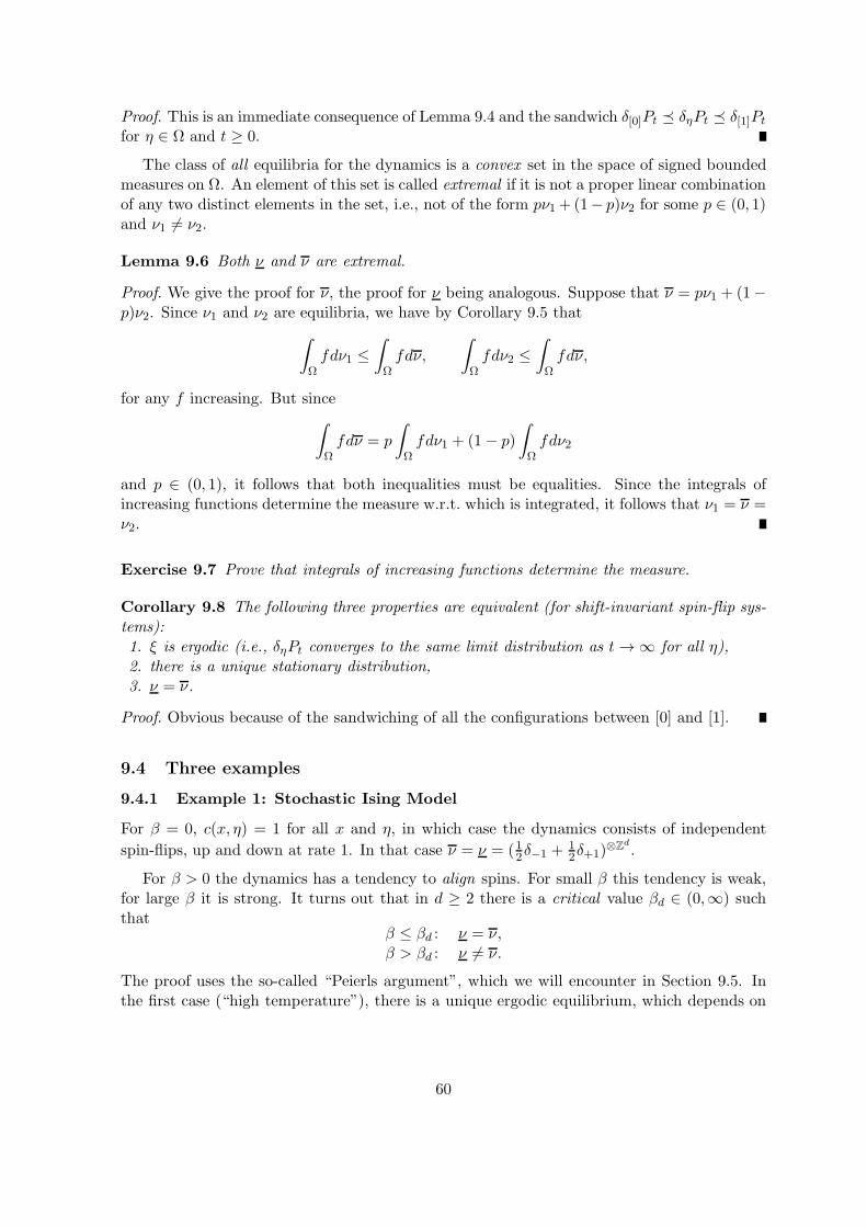
Proof. This is an immediate consequence of Lemma 9.4 and the sandwich δ[0]Pt δηPt δ[1]Pt
for η ∈ Ω and t ≥ 0.
The class of all equilibria for the dynamics is a convex set in the space of signed boundedmeasures on Ω. An element of this set is called extremal if it is not a proper linear combinationof any two distinct elements in the set, i.e., not of the form pν1 +(1− p)ν2 for some p ∈ (0, 1)and ν1 6= ν2.
Lemma 9.6 Both ν and ν are extremal.
Proof. We give the proof for ν, the proof for ν being analogous. Suppose that ν = pν1 + (1−p)ν2. Since ν1 and ν2 are equilibria, we have by Corollary 9.5 that
∫
Ωfdν1 ≤
∫
Ωfdν,
∫
Ωfdν2 ≤
∫
Ωfdν,
for any f increasing. But since
∫
Ωfdν = p
∫
Ωfdν1 + (1− p)
∫
Ωfdν2
and p ∈ (0, 1), it follows that both inequalities must be equalities. Since the integrals ofincreasing functions determine the measure w.r.t. which is integrated, it follows that ν1 = ν =ν2.
Exercise 9.7 Prove that integrals of increasing functions determine the measure.
Corollary 9.8 The following three properties are equivalent (for shift-invariant spin-flip sys-tems):1. ξ is ergodic (i.e., δηPt converges to the same limit distribution as t→∞ for all η),2. there is a unique stationary distribution,3. ν = ν.
Proof. Obvious because of the sandwiching of all the configurations between [0] and [1].
9.4 Three examples
9.4.1 Example 1: Stochastic Ising Model
For β = 0, c(x, η) = 1 for all x and η, in which case the dynamics consists of independent
spin-flips, up and down at rate 1. In that case ν = ν = (12δ−1 +12δ+1)
⊗Zd.
For β > 0 the dynamics has a tendency to align spins. For small β this tendency is weak,for large β it is strong. It turns out that in d ≥ 2 there is a critical value βd ∈ (0,∞) suchthat
β ≤ βd : ν = ν,β > βd : ν 6= ν.
The proof uses the so-called “Peierls argument”, which we will encounter in Section 9.5. Inthe first case (“high temperature”), there is a unique ergodic equilibrium, which depends on
60

β and is denoted by νβ. In the second case (“low temperature”), there are two extremalequilibria, both of which depend on β and are denoted by
ν+β = “plus state” with∫Ω η(0)ν
+β (dη) > 0,
ν−β = “minus-state” with∫Ω η(0)ν
+β (dη) < 0,
which are called the magnetized states. Note that ν+β and ν−β are images of each other underthe swapping of +1’s and −1’s. It can be shown that in d = 2 all equilibria are a convexcombination of ν+β and ν−β , while in d ≥ 3 also other equilibria are possible (e.g. not shift-invariant) when β is large enough. It turns out that β1 = 0, i.e., in d = 1 the SIM is ergodicfor all β > 0.
9.4.2 Example 2: Contact Process
Note that [0] is a trap for the dynamics (if all sites are healthy, then no infection will everoccur), and so
ν = δ[0].
For small λ infection is transmitted slowly, for large λ rapidly. It turns out that in d ≥ 1 thereis a critical value λd ∈ (0,∞) such that
λ ≤ λd : ν = δ[0] (“extinction”, no epidemic),
λ > λd : ν 6= δ[0] (“survival”, epidemic).
Lemma 9.9 (i) dλd ≤ λ1,(ii) 2dλd ≥ 1,(iii) λ1 <∞.
The proof of this lemma will be given in Section 9.5. It uses a number of comparisonarguments based on coupling. Note that (i–iii) combine to yield that 0 < λd <∞ for all d ≥ 1,so that the phase transition occurs at a non-trivial value of the infection rate parameter.
Remark: Sharp estimates are available for λ1, but these require heavy machinery. Also, aseries expansion of λd in powers of 1/2d is known up to several orders, but again the proof isvery technical.
9.4.3 Example 3: Voter Model
Note that [0] and [1] are both traps for the dynamics (if all sites have the same opinion, thenno change of opinion occurs), and so
ν = δ[0], ν = δ[1].
It turns out that in d = 1, 2 these are the only extremal equilibria, while in d ≥ 3 there is a1-parameter family of extremal equilibria
(νρ)ρ∈[0,1]
with ρ the density of 1’s, i.e., νρ(η(0) = 1) = ρ. This is remarkable because the VM hasno parameter to play with. For ρ = 0 and ρ = 1 these equilibria coincide with δ[0] and δ[1],respectively.
Remark: The dichotomy d = 1, 2 versus d ≥ 3 is directly related to simple random walkbeing recurrent in d = 1, 2 and transient in d ≥ 3.
61
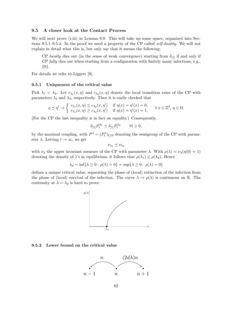
9.5 A closer look at the Contact Process
We will next prove (i-iii) in Lemma 9.9. This will take up some space, organized into Sec-tions 9.5.1–9.5.4. In the proof we need a property of the CP called self-duality. We will notexplain in detail what this is, but only say that it means the following:
CP locally dies out (in the sense of weak convergence) starting from δ[1] if and only ifCP fully dies out when starting from a configuration with finitely many infections, e.g.,0.
For details we refer to Liggett [9].
9.5.1 Uniqueness of the critical value
Pick λ1 < λ2. Let cλ1(x, η) and cλ2
(x, η) denote the local transition rates of the CP withparameters λ1 and λ2, respectively. Then it is easily checked that
η η′ →cλ1
(x, η) ≤ cλ2(x, η′) if η(x) = η′(x) = 0,
cλ1(x, η) ≥ cλ2
(x, η′) if η(x) = η′(x) = 1,∀x ∈ Zd, η ∈ Ω.
(For the CP the last inequality is in fact an equality.) Consequently,
δ[1]Pλ1t δ[1]P λ2
t ∀t ≥ 0,
by the maximal coupling, with P λ = (P λt )t≥0 denoting the semigroup of the CP with param-
eter λ. Letting t→∞, we getνλ1 νλ2
with νλ the upper invariant measure of the CP with parameter λ. With ρ(λ) = νλ(η(0) = 1)denoting the density of 1’s in equilibrium, it follows that ρ(λ1) ≤ ρ(λ2). Hence
λd = infλ ≥ 0: ρ(λ) > 0 = supλ ≥ 0: ρ(λ) = 0defines a unique critical value, separating the phase of (local) extinction of the infection fromthe phase of (local) survival of the infection. The curve λ 7→ ρ(λ) is continuous on R. Thecontinuity at λ = λd is hard to prove.
9.5.2 Lower bound on the critical value
62
Pick A0 finite and consider the CP in dimension d with parameter λ starting from the set A0
as the set of infected sites. Let A = (At)t≥0 with At the set of infected sites at time t. Then
|At| decreases by 1 at rate |At|,|At| increases by 1 at rate ≤ 2dλ|At|,
where the latter holds because each site in At has at most 2d non-infected neighbors. Nowconsider the two random process X = (Xt)t≥0 with Xt = |At| and Y = (Yt)t≥0 given by thebirth-death process on N0 that moves at rate n from n to n − 1 (death) and at rate (2dλ)nfrom n to n + 1 (birth), both starting from n0 = |A0|. Then X and Y can be coupled suchthat
P(Xt ≤ Yt ∀ t ≥ 0) = 1,
where P denotes the coupling measure. Note that n = 0 is a trap for both X and Y . If2dλ < 1, then this trap is hit with probability 1 by Y , i.e., limt→∞ Yt = 0 a.s., and hence alsoby X, i.e., limt→∞Xt = 0 a.s. Therefore νλ = δ[0] when 2dλ < 1. Consequently, 2dλd ≥ 1.
9.5.3 Upper bound on the critical value
The idea is to couple two CP’s that live in dimensions 1 and d. Again, let A = (At)t≥0 withAt the set of infected sites at time t of the CP in dimension d with parameter λ, this timestarting from A0 = 0. Let B = (Bt)t≥0 be the same as A, but for the CP in dimension 1with parameter λd, starting from B0 = 0.
Define the projection πd : Zd → Z as
πd(x1, . . . , xd) = x1 + · · ·+ xd.
We will construct a coupling P of A and B such that
P(Bt ⊆ πd(At) ∀ t ≥ 0) = 1.
From this we get
P(At 6= ∅ | A0 = 0
)= P
(πd(At) 6= ∅ | A0 = 0
)≥ P
(Bt 6= ∅ | B0 = 0
),
which implies that if A dies out then also B dies out. In other words, if λ ≤ λd, then λd ≤ λ1,which implies that dλd ≤ λ1 as claimed.
The construction of the coupling is as follows. Fix t ≥ 0. Suppose that At = A and Bt = Bwith B ⊂ πd(A). For each y ∈ B there is at least one x ∈ A with y = πd(x). Pick one such xfor every y (e.g. choose the closest up or the closest down). Now couple:
– If x becomes healthy, then y becomes healthy too.– If x infects any of the d sites x− ei with i = 1, . . . , d, then y infects y − 1.– If x infects any of the d sites x+ ei with i = 1, . . . , d, then y infects y + 1.– Anything that occurs at other x′’s such that πd(x
′) = y, has no effect on y.
(This is a mapping that defines how Bt evolves given how At evolves.)
Exercise 9.10 Check that this coupling has the right marginals and preserves the inclusionBt ⊆ πd(At).
Since A0 = B0 = 0 and 0 ⊂ πd(0), the proof is complete.
63
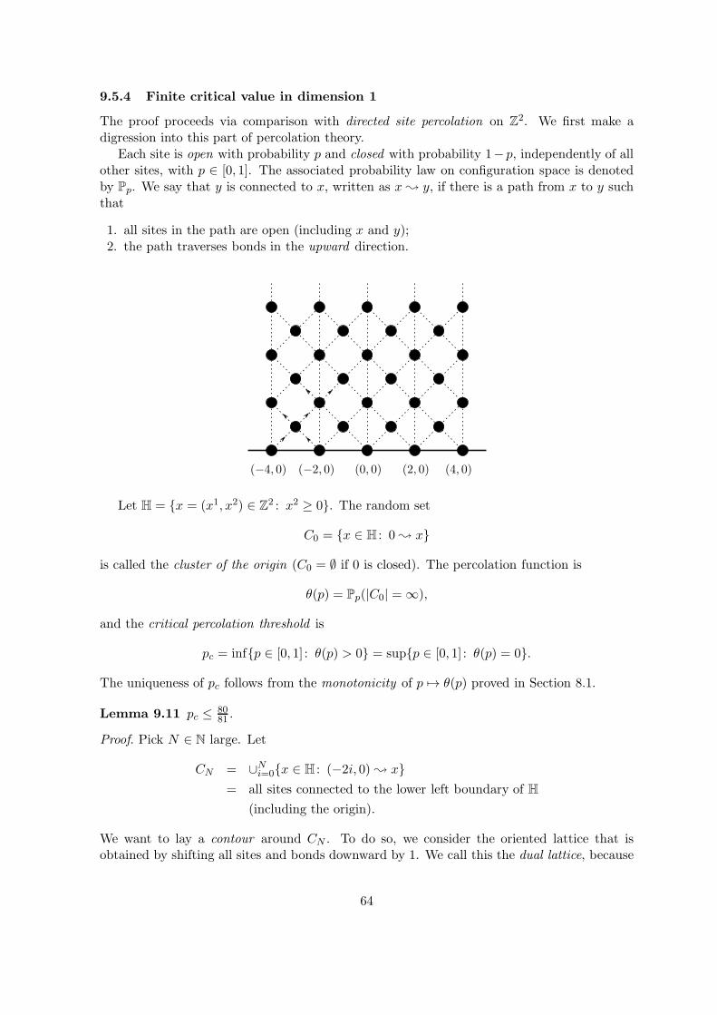
9.5.4 Finite critical value in dimension 1
The proof proceeds via comparison with directed site percolation on Z2. We first make adigression into this part of percolation theory.
Each site is open with probability p and closed with probability 1− p, independently of allother sites, with p ∈ [0, 1]. The associated probability law on configuration space is denotedby Pp. We say that y is connected to x, written as x; y, if there is a path from x to y suchthat
1. all sites in the path are open (including x and y);2. the path traverses bonds in the upward direction.
Let H = x = (x1, x2) ∈ Z2 : x2 ≥ 0. The random set
C0 = x ∈ H : 0 ; x
is called the cluster of the origin (C0 = ∅ if 0 is closed). The percolation function is
θ(p) = Pp(|C0| =∞),
and the critical percolation threshold is
pc = infp ∈ [0, 1] : θ(p) > 0 = supp ∈ [0, 1] : θ(p) = 0.
The uniqueness of pc follows from the monotonicity of p 7→ θ(p) proved in Section 8.1.
Lemma 9.11 pc ≤ 8081 .
Proof. Pick N ∈ N large. Let
CN = ∪Ni=0x ∈ H : (−2i, 0) ; x= all sites connected to the lower left boundary of H
(including the origin).
We want to lay a contour around CN . To do so, we consider the oriented lattice that isobtained by shifting all sites and bonds downward by 1. We call this the dual lattice, because
64

the two lattices together make up Z2 (with upward orientation). Now define
ΓN = the exterior boundary of the set of all faces in the dual lattice
containing a site of CN or one of the boundary sites(−2i+ 1,−1),with i = 1, . . . , N.
Think of ΓN as a path from (0,−1) to (−2N,−1) in the dual lattice, enclosing CN andbeing allowed to cross bonds in both directions. We call ΓN the contour of CN (this contourmay be infinite). We need the following observations:
(i) There are at most 4 3n−2 contours of length n.(ii) Any contour of length n has at least n/4 closed sites adjacent to it on the outside.
Exercise 9.12 Prove the observations above.
We can now complete the proof as follows. Since the shortest possible contour has length2N , it follows from (i) and (ii) that
Pp(|CN | <∞) = Pp(|ΓN | <∞) ≤∞∑
n=2N
4 3n−2(1− p)n/4.
If p > 80/81, then 3(1− p)1/4 < 1 and the sum is < 1 for N sufficiently large, i.e., Pp(|CN | =∞) > 0 for N ≥ N0(p). Using the translation invariance, we have
Pp(|CN | =∞) ≤ (N + 1)Pp(|C0| =∞).
Hence, if p > 80/81, then Pp(|C0| =∞) > 0, which implies that pc ≤ 80/81.
The contour argument above is referred to as a Peierls argument. A similar argumentworks for many other models as well (such as SIM).
65
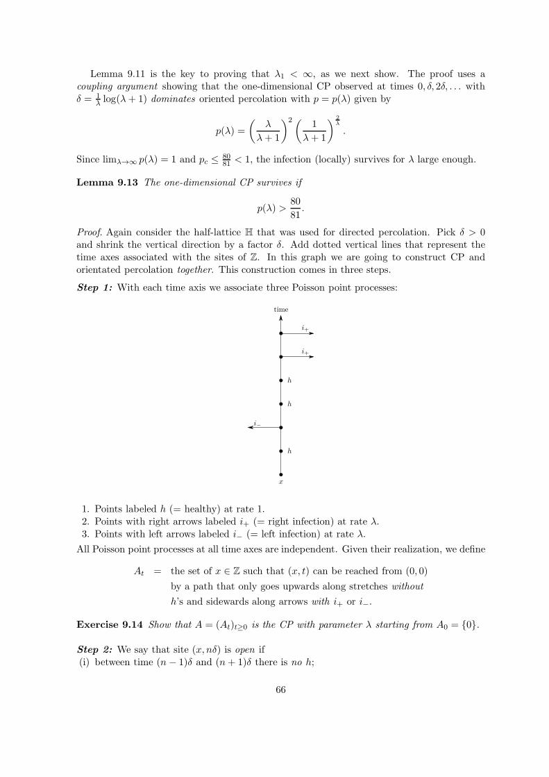
Lemma 9.11 is the key to proving that λ1 < ∞, as we next show. The proof uses acoupling argument showing that the one-dimensional CP observed at times 0, δ, 2δ, . . . withδ = 1
λ log(λ+ 1) dominates oriented percolation with p = p(λ) given by
p(λ) =
(λ
λ+ 1
)2( 1
λ+ 1
) 2λ
.
Since limλ→∞ p(λ) = 1 and pc ≤ 8081 < 1, the infection (locally) survives for λ large enough.
Lemma 9.13 The one-dimensional CP survives if
p(λ) >80
81.
Proof. Again consider the half-lattice H that was used for directed percolation. Pick δ > 0and shrink the vertical direction by a factor δ. Add dotted vertical lines that represent thetime axes associated with the sites of Z. In this graph we are going to construct CP andorientated percolation together. This construction comes in three steps.
Step 1: With each time axis we associate three Poisson point processes:
1. Points labeled h (= healthy) at rate 1.2. Points with right arrows labeled i+ (= right infection) at rate λ.3. Points with left arrows labeled i− (= left infection) at rate λ.
All Poisson point processes at all time axes are independent. Given their realization, we define
At = the set of x ∈ Z such that (x, t) can be reached from (0, 0)
by a path that only goes upwards along stretches without
h’s and sidewards along arrows with i+ or i−.
Exercise 9.14 Show that A = (At)t≥0 is the CP with parameter λ starting from A0 = 0.
Step 2: We say that site (x, nδ) is open if(i) between time (n − 1)δ and (n+ 1)δ there is no h;
66

(ii) between time nδ and (n+ 1)δ there are both an i+ and an i−.Define
Bnδ = the set of x ∈ Z such that 0 ; (x, nδ).
Exercise 9.15 Show that Bnδ = x ∈ Z : (x, nδ) ∈ C0, where C0 is the cluster at the originin orientated percolation with p = e−2δ(1− e−δλ)2.
Step 3: The key part of the coupling is
Anδ ⊃ Bnδ ∀n ∈ N0.
Exercise 9.16 Prove this inclusion.
Let P denote the joint law of the three Poisson point processes at all the sites. By combiningSteps 1–3 and noting that
P(Anδ 6= ∅ ∀n ∈ N0 | A0 = 0
)≥ P
(Bnδ 6= ∅ ∀n ∈ N0 | B0 = 0
)
= Pp(|C0| =∞),
we obtain, with the help of Fact 9.11, that the one-dimensional CP with parameter λ survivesif
supδ>0
e−2δ(1− e−δλ)2 >80
81,
where in the left-hand side we optimize over δ, which is allowed because the previous estimateshold for all δ > 0. The supremum is attained at
δ =1
λlog(λ+ 1),
which yields the claim in Fact 9.13.
Since limλ→∞ p(λ) = 1, it follows from Lemma 9.13 that λ1 <∞.
Remark: The bound in Lemma 9.13 yields λ1 ≤ 1318. This is a large number because theestimates that were made are crude. The true value is λ1 ≈ 1.6494, based on simulations andapproximation techniques.
67
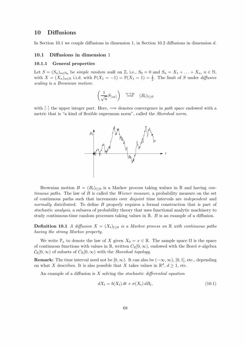
10 Diffusions
In Section 10.1 we couple diffusions in dimension 1, in Section 10.2 diffusions in dimension d.
10.1 Diffusions in dimension 1
10.1.1 General properties
Let S = (Sn)n∈N0be simple random walk on Z, i.e., S0 = 0 and Sn = X1 + . . . +Xn, n ∈ N,
with X = (Xn)n∈N i.i.d. with P(X1 = −1) = P(X1 = 1) = 12 . The limit of S under diffusive
scaling is a Brownian motion:
(1√nS⌈nt⌉
)n→∞=⇒ (Bt)t≥0
with ⌈·⌉ the upper integer part. Here, =⇒ denotes convergence in path space endowed with ametric that is “a kind of flexible supremum norm”, called the Skorohod norm.
Brownian motion B = (Bt)t≥0 is a Markov process taking walues in R and having con-tinuous paths. The law of B is called the Wiener measure, a probability measure on the setof continuous paths such that increments over disjoint time intervals are independent andnormally distributed. To define B properly requires a formal construction that is part ofstochastic analysis, a subarea of probability theory that uses functional analytic machinery tostudy continuous-time random processes taking values in R. B is an example of a diffusion.
Definition 10.1 A diffusion X = (Xt)t≥0 is a Markov process on R with continuous pathshaving the strong Markov property.
We write Px to denote the law of X given X0 = x ∈ R. The sample space Ω is the spaceof continuous functions with values in R, written CR[0,∞), endowed with the Borel σ-algebraCR[0,∞) of subsets of CR[0,∞) with the Skorohod topology.
Remark: The time interval need not be [0,∞). It can also be (−∞,∞), [0, 1], etc., dependingon what X describes. It is also possible that X takes values in Rd, d ≥ 1, etc.
An example of a diffusion is X solving the stochastic differential equation
dXt = b(Xt) dt+ σ(Xt) dBt, (10.1)
68
where b(Xt) denotes the local drift function and σ(Xt) the dispersion function. The integralform of (10.1) reads
Xt = X0 +
∫ t
0b(Xs) ds+
∫ t
oσ(Xs) dBs,
where the last integral is a so-called “Ito-integral”. Equation (10.1) is short-hand for thestatement:
The increments of X over the infinitesimal time interval [t, t+ dt) is a sum of twoparts, b(Xt)dt and σ(Xt)dBt, with dBt the increment of B over the same timeinterval.
Again, a formal definition of (10.1) requires functional analytic machinery. The functionsb : R → R and σ : R → R need to satisfy mild regularity properties, e.g. locally Lipschitzcontinuous and modest growth at infinity. The solution of (10.1) is called an Ito-diffusion.The special case with b ≡ 0, σ ≡ 1 is Brownian motion itself. The interpretation of X is:
X is a Brownian motion whose increments are blown up by a factor σ(·) andshifted by a factor b(·), both of which depend on the value of the process itself.
Definition 10.2 A diffusion is called regular if
Px(τy <∞) > 0 ∀x, y ∈ R
with τy = inft ∈ [0,∞) : Xt = y the hitting time of y.
Regularity is analogous to irreducibility for Markov processes taking values in countablestate spaces. Every regular diffusion has the property
Px(τb < τa) =s(x)− s(a)s(b)− s(a) ∀ a, b ∈ R, a < x < b,
for some s : R → R continuous and strictly increasing. This s is called the scale function forX. A diffusion is “in natural scale” when s is the identity. An example of such a diffusion isBrownian motion B. More generally, Y = (Yt)t≥0 with Yt = s(Xt) is in natural scale, and isan Ito-diffusion with b ≡ 0.
Exercise 10.3 Check the last claim.
Definition 10.4 A diffusion is called recurrent if
Px(τy <∞) = 1 ∀x, y ∈ R.
10.1.2 Coupling on the half-line
For recurrent diffusions on the half-line we have a successful coupling starting from any twostarting points. Indeed, let
T = inft ∈ [0,∞) : Xt = X ′t
be the coupling time of X = (Xt)t≥0 and X ′ = (X ′t)t≥0. Because X and X ′ are continuous
(“skip-free”), we haveT ≤ τ0 ∨ τ ′0,
69
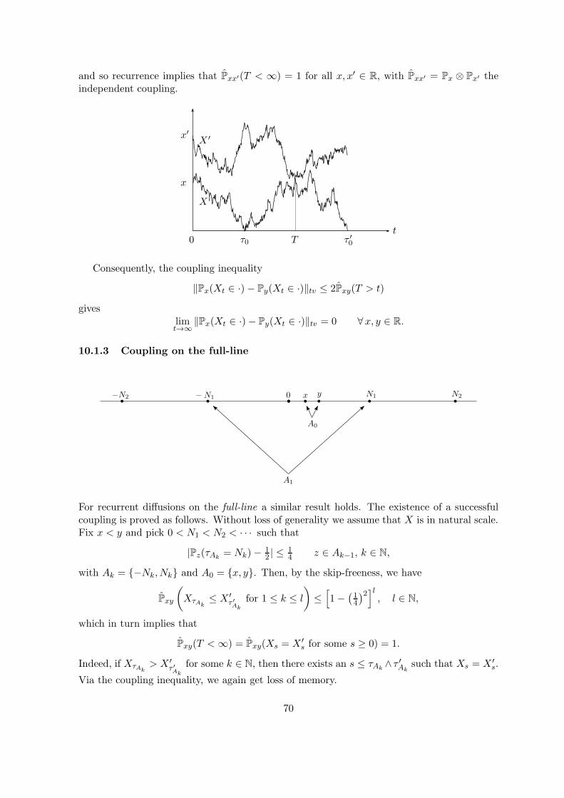
and so recurrence implies that Pxx′(T < ∞) = 1 for all x, x′ ∈ R, with Pxx′ = Px ⊗ Px′ theindependent coupling.
Consequently, the coupling inequality
‖Px(Xt ∈ ·)− Py(Xt ∈ ·)‖tv ≤ 2Pxy(T > t)
giveslimt→∞‖Px(Xt ∈ ·)− Py(Xt ∈ ·)‖tv = 0 ∀x, y ∈ R.
10.1.3 Coupling on the full-line
For recurrent diffusions on the full-line a similar result holds. The existence of a successfulcoupling is proved as follows. Without loss of generality we assume that X is in natural scale.Fix x < y and pick 0 < N1 < N2 < · · · such that
|Pz(τAk= Nk)− 1
2 | ≤ 14 z ∈ Ak−1, k ∈ N,
with Ak = −Nk, Nk and A0 = x, y. Then, by the skip-freeness, we have
Pxy
(XτAk
≤ X ′τ ′Ak
for 1 ≤ k ≤ l)≤[1−
(14
)2]l, l ∈ N,
which in turn implies that
Pxy(T <∞) = Pxy(Xs = X ′s for some s ≥ 0) = 1.
Indeed, if XτAk> X ′
τ ′Ak
for some k ∈ N, then there exists an s ≤ τAk∧ τ ′Ak
such that Xs = X ′s.
Via the coupling inequality, we again get loss of memory.
70

Theorem 10.5 Regular diffusions X have the strong Feller property, i.e., for any boundedf : R→ R and any t > 0, the function Ptf defined by
(Ptf)(x) = Ex[f(Xt)], x ∈ R,
is continuous.
Proof. Fix t > 0. Let X and X ′ be independent copies of the diffusion starting from x and x′,respectively. Then
∣∣(Ptf)(x)− (Ptf)(x′)∣∣ =
∣∣∣Exx′[f(Xt)]− Exx′[f(X ′t)∣∣∣
≤ 2Pxx′(T > t) ‖f‖∞.
The claim follows from the fact that
limx′→x
Pxx′(T > t) = 0 ∀ t > 0,
which is intuitively obvious.
Exercise 10.6 Prove the latter statement by using an argument of the type given for thesuccessful coupling on the full-line, but now with shrinking rather than growing intervals.
The Feller property is important because it says that the space of bounded continuousfunctions is preserved by the semigroup P = (Pt)t≥0. Since this set is dense in the space ofcontinuous functions, the Feller property allows us to control very large sets of functionals ofdiffusions.
Theorem 10.7 Let P = (Pt)t≥0 be the semigroup of a regular diffusion. Then
λ ≤ µ =⇒ λPt ≤ µPt ∀ t ≥ 0.
Proof. This is immediate from the skip-freeness, by which λ ≤ µ allows X0 ≤ X ′0, and hence
Xt ≤ X ′t for all t ≥ 0, when X0,X
′0 start from λ, µ.
10.2 Diffusions in dimension d
Let S = (Sn)n∈N be simple random walk on Zd, d ≥ 1: S0 = 0, Sn = X1 + · · · +Xn, n ∈ N,with X = (Xn)n∈N i.i.d. with P(X1 = −ei) = P(X1 = ei) =
12d , i = 1 . . . , d, where e1, . . . , ed
are the unit vectors in Zd.The limit of S under diffusive scaling is Brownian motion on Rd:
(1√nS⌈nt⌉
)n→∞=⇒ (Bt)t≥0,
where the right-hand side is Markov process with values in Rd and with continuous paths. Infact,
Bt = (B1t , . . . , B
nt )
such that the d components form independent Brownian motions on R (moving at 1/d timesthe rate of one-dimensional Brownian motion). The main definitions of what a diffusion is onRd carry over from d = 1. Regularity becomes
Px(τBǫ(y) <∞) > 0 ∀x, y ∈ Rd, ǫ > 0,
71
and recurrence becomes
Px(τBǫ(y) <∞) = 1 ∀x, y ∈ Rd, ǫ > 0,
i.e., points are replaced by small balls around points in all statements about hitting times.Ito-diffusions are defined by
dXt = b(Xt) dt+ σ(Xt) dBt, (10.2)
where b : Rd → Rd and σ : RdRd×Rd are the vector local drift function and the matrix localdispersion function, both subject to regularity properties.
Diffusions in Rd, d ≥ 2, are more difficult to analyze than in R. A lot is known for specialclasses of diffusions (e.g. with certain symmetry properties). Stochastic analysis has developeda vast arsenal of ideas, results and techniques. The stochastic differential equation in (10.2) isvery important because it has a wide range of application, e.g. in transport, finance, filtering,coding, statistics, genetics, etc.
72
References
[1] O. Angel, J. Goodman, F. den Hollander and G. Slade, Invasion percolation on regulartrees, Annals of Probability 36 (2008) 420–466.
[2] A.D. Barbour, L. Holst and S. Janson, Poisson Approximation, Oxford Studies in Prob-ability 2, Clarendon Press, Oxford, 1992.
[3] P. Diaconis, The cutoff phenomenon in finite Markov chains, Proc. Natl. Acad. Sci. USA93 (1996) 1659–1664.
[4] G.R. Grimmett, Percolation, Springer, Berlin, 1989.
[5] O. Haggstrom, Finite Markov Chains and Algorithmic Applications, London Mathemat-ical Society Student Texts 52, Cambridge University Press, Cambridge, 2002.
[6] F. den Hollander and M.S. Keane, Inequalities of FKG type, Physica 138A (1986) 167–182.
[7] C. Kraaikamp, Markov Chains: an introduction, lecture notes TU Delft, 2010.
[8] D.A. Levin, Y. Peres and E.L. Wilmer, Markov Chains and Mixing Times, AmericanMathematical Society, Providence RI, 2009.
[9] T.M. Liggett, Interacting Particle Systems, Grundlehren der mathematische Wis-senschaften 276, Springer, New York, 1985.
[10] T. Lindvall, W. Doeblin 1915–1940, Annals of Probability 19 (1991) 929–934.
[11] T. Lindvall, Lectures on the Coupling Method, John Wiley & Sons, New York, 1992.Reprint: Dover paperback edition, 2002.
[12] H. Nooitgedagt, Two convergence limits of Markov chains: Cut-off and Metastability,MSc thesis, Mathematical Institute, Leiden University, 31 August 2010.
[13] J.A. Rice, Mathematical Statistics and Data Analysis (3rd edition), Duxbury AdvancedSeries, Thomson Brooks/Cole, Belmont, California, 2007.
[14] F. Spitzer, Principles of Random Walk, Springer, New York, 1976.
[15] H. Thorisson, Coupling, Stationarity and Regeneration, Springer, New York, 2000.
73