Probability and Statistics

2141-375 Measurement and Instrumentation

Statistical Measurement Theory

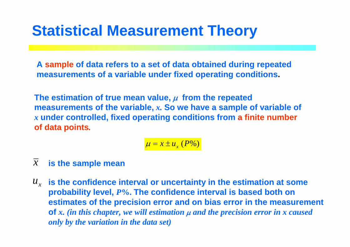
A sample of data refers to a set of data obtained during repeate d measurements of a variable under fixed operating cond itions .

The estimation of true mean value, µµµµ from the repeated measurements of the variable, x. So we have a sample of variable ofx under controlled, fixed operating conditions from a finite number of data points.

%)( Pux x±=µ

x is the sample mean

xu is the confidence interval or uncertainty in the estim ation at some probability level, P%. The confidence interval is based both on estimates of the precision error and on bias error in the measurement of x. (in this chapter, we will estimation µµµµ and the precision error in x caused only by the variation in the data set)

Infinite Statistics: Normal Distribution

µµµµ is the true mean and σσσσ2 is the true variance of x

A common distribution found in measurements e.g. th e measurement of length, temperature, pressure etc.

])(

2

1exp[

2

1)(

2

2

σµ

πσ−

−=x

xp

The probability density function for a random varia ble, x having normal distribution is defined as

The probability, P(x) within the interval a and b is given by the area under p(x)

∫=≤≤b

a

dxxpbxaP )()(

),(~ 2σµNX

Notation for random variable X has a normal distribution with mean µµµµ and σσσσvariance

The Standard Normal Distribution

for -∞∞∞∞ ≤≤≤≤ x ≤≤≤≤ ∞∞∞∞

The standard normal distribution:

]2

1exp[

2

1)( 2xxp −=

π

The cumulative distribution function of a standard normal distribution

The Normal error function

∫ −=≤≤a

dxx

axP0

2

]2

exp[2

1)0(

π

)1,0(~ NX

The probability density function has the notation, p(x)

dyypxPx

)()( ∫ ∞−= ∫

∞−

−=≤≤−∞a

dxx

axP ]2

exp[2

1)(

2

π

The Standard Normal Distribution

-3 -2 -1 0 1 2 3

]2

1exp[

2

1)( 2xxp −=

π

)1,0(N

1=σ 1=σ

∫∞−

−=x

dzzxP ]2

1exp[

2

1)( 2

π

-3 -2 -1 0 1 2 3

0.5

1

The standard normal distribution The cumulative distribution of the standard normal distribution

0=µ

x x

T h e S t a n d a r d N o r m a l D i s t r i b u t i o n

N(0,1)

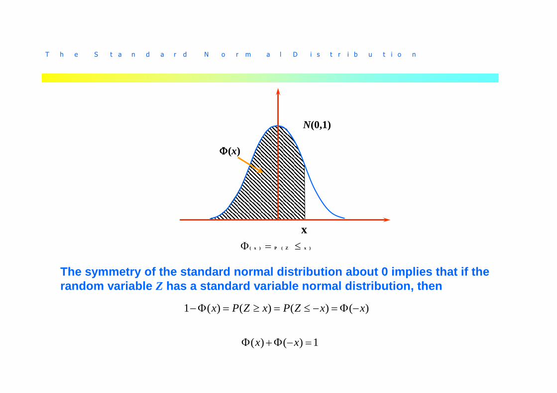
ΦΦΦΦ(x)

x)()( xZPx ≤=Φ

The symmetry of the standard normal distribution ab out 0 implies that if the random variable Z has a standard variable normal distribution, then

)()()()(1 xxZPxZPx −Φ=−≤=≥=Φ−

1)()( =−Φ+Φ xx

Probability Calculations for Normal Distribution

If X ~ N(µµµµ,σσσσ2), then

−≤−

−≤=≤≤

σµ

σµ a

ZPb

ZPbxaP )(

The random variable Z is known as the “standardized” version of the random variable, X. This results implies that the probability values o f a general normal distribution can be related to the cumulative distr ibution of the standard normal distribution ΦΦΦΦ(x) through the relation

)1,0(~ NX

Zσµ−

=

−Φ−

−Φ=

σµ

σµ ab

The Normal Distribution

-3 -2 -1 0 1 2 3

)(xp

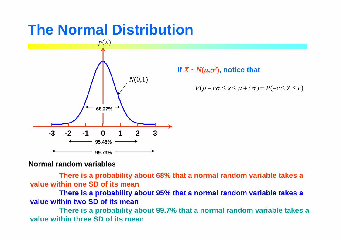
68.27%

95.45%

99.73%

N(0,1)

There is a probability about 68% that a normal rand om variable takes a value within one SD of its mean

There is a probability about 95% that a normal rand om variable takes a value within two SD of its mean

There is a probability about 99.7% that a normal ra ndom variable takes a value within three SD of its mean

Normal random variables

)()( cZcPcxcP ≤≤−=+≤≤− σµσµ

If X ~ N(µµµµ,σσσσ2), notice that

The Normal Distribution

Example: It is known that the statistics of a well-defined voltage signal are given by µ = 8.5 V and σ2 = 2.25 V2. If a single measurement of the voltage signal is made, determine the probability that the measured value will be between 10.0 and 11.5 V

Known: µµµµ = 8.5 V and σσσσ2 = 2.25 V2

P(10.0 ≤ x ≤ 11.5) = P(x ≤ 11.5) –P(x ≤ 10.0)

Solution:

Assume: Signal has a normal distribution

P(10.0 ≤ x ≤ 11.5) = 0.1359

=P[Z ≤ (11.5-8.5)/1.5] –P[Z ≤ (10.0-8.5)/1.5]

=P[Z ≤ 2] – P[Z ≤ 1]

=0.9772 – 0.8413

Finite Statistics: Sample Versus Population

Population Sample

Populationparameters

Samplestatistics

StatisticalInference

Randomselection

(experiment)

The finite sample versus the infinite population

Parameter is a quantity that is a property of unkno wn probability distribution. This may be the mean, variance or a particular quantity.

Statistic is a quantity that is a property of sampl e. This may be the mean, variance or a particular quantity. Statistics can be calcula ted from a set of data observations.

Estimation is a procedure by which the information contained within a sample is used to investigate properties of the population fr om which the sample is drawn.

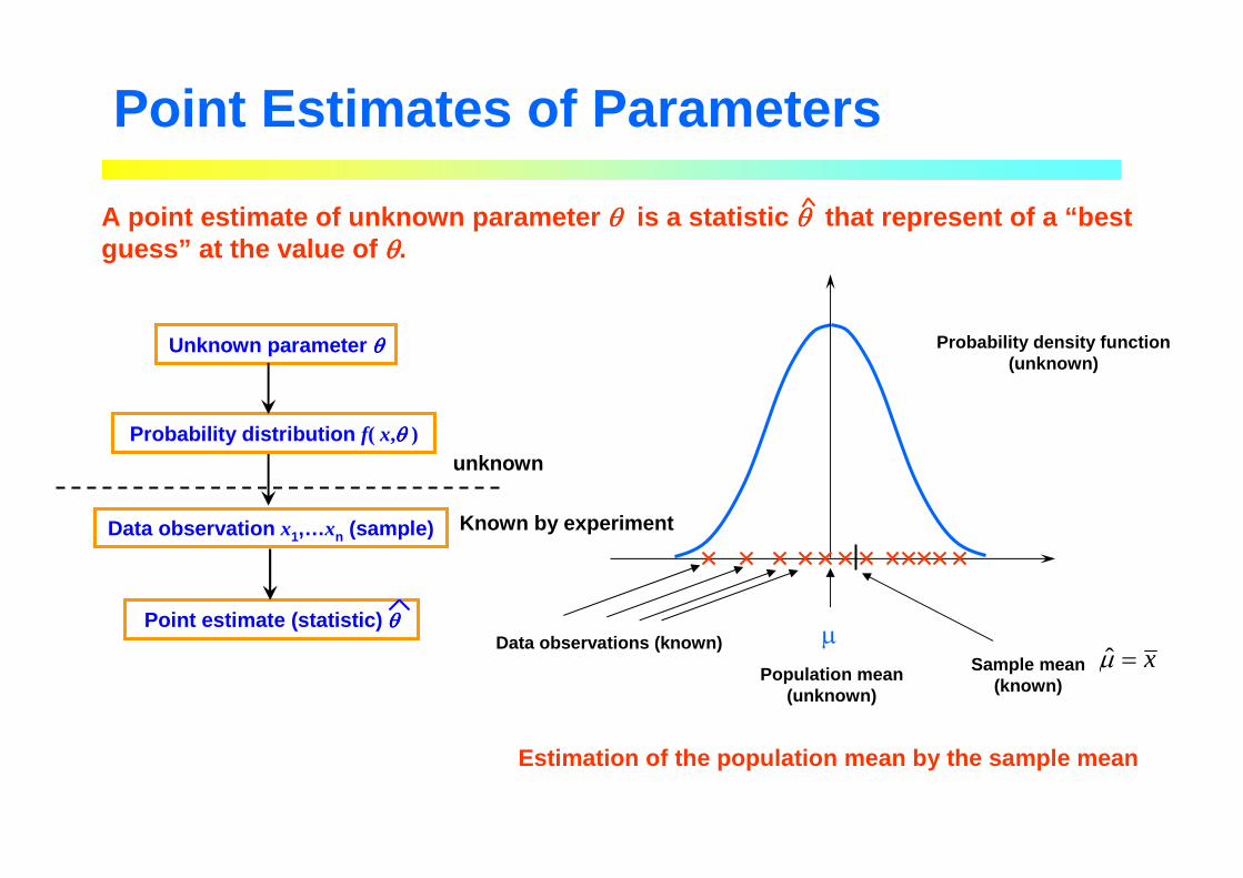
Population mean(unknown)

µData observations (known)Sample mean

(known)x=µ̂

Probability density function(unknown)

Point Estimates of Parameters

A point estimate of unknown parameter θθθθ is a statistic θθθθ that represent of a “best guess” at the value of θθθθ.

Estimation of the population mean by the sample mea n

Unknown parameter θθθθ

Probability distribution f( x,θθθθ )

Data observation x1,…xn (sample)

Point estimate (statistic) θθθθ

unknown

Known by experiment

Point Estimation of Mean and Variance

Sample mean: Point Estimate of a Population Mean

∑=

==N

iix

Nx

1

1µ̂

( )∑=

−−

==N

iix xx

NS

1

222

1

1σ̂

If X1, …, Xn is a sample of observation from a probability distr ibution which a mean µµµµ, then the sample mean

is the best guess of the point estimate of the popu lation mean µµµµ

Sample variance: Point Estimate of a Population Vari ance:

If X1, …, Xn is a sample of observation from a probability distr ibution which a variance σσσσ2, then the sample variance

is the best guess of the point estimate of the popu lation variance σσσσ2

Inference of Population Mean

%)( , PStxx xPvi ±∈

Where the variable tv,p is a function of the probability P, and the degree of freedom v = n - 1 of the Student- t distribution.

The estimate of the true mean value based on a fini te data set is

For a normal distribution of x about some sample mean value, x one can state that

( ) ( ) or , ,,,, xPvxPvxPvxPv Stx,n/StxStxStx +−∈+−∈ µµ

The standard deviation of the mean

N

SS x

x =

Inference of Population Mean

( ) %)( , Puxux xx +−∈µ

x

µ̂

xux − xux +

Precision error ux

with confident level P or 1 -αααα

Inference methods on a population mean based on the t-procedure for large sample size n ≥≥≥≥ 30 and also for small sample sizes as long as the data can reasonably be taken to be approximately normally di stributed. Nonparametric techniques can be employed for small sample sizes w ith data that are clearly not normally distributed

Example: Consider the data in the table below. (a) Compute the sample statistics for this data set. (b) Estimate the interval of values over which 95% of the measurements of the measurand should be expected to lie. (c) Estimate the true mean value of the measurand at 95% probability based on this finite data set

Known: the given table, N = 20

Solution:

Assume: data set follows a normal distribution

Inference of Population Mean

i x i i x i

1 0.98 11 1.022 1.07 12 1.263 0.86 13 1.084 1.16 14 1.025 0.96 15 0.946 0.68 16 1.117 1.34 17 0.998 1.04 18 0.789 1.21 19 1.06

10 0.86 20 0.96

Inference of Population Variance

222 /~ σχ xvS

with the degree of freedom v = n - 1

For a normal distribution of x, sample variance S 2 has a probability density function of chi-square χχχχ2

Precision Interval in a Sample Variance

ααα −=≤≤ 1)χχχ( 2/2

22/2-1P

ασ αα −=≤≤ 1)/χ/χ( 2/2-1

222/2

2xx vSvSP

)1( )/χ,/χ( 2/2-1

22/2

22 ασ αα −=∈ PvSvS xx

with a probability of P(χχχχ2) = 1-αααα

Example: Ten steel tension specimens are tested from a large batch, and a sample variance of (200 kN/m2)2 is found. State the true variance expected at 95% confidence.

Known: S 2 = 40000 (kN/m2)2, N = 10

Solution: assume data set follows a normal distrib ution, with v = n - 1 = 9

Inference of Population Variance

From chi-square table χχχχ2 = 19 at αααα = 0.025 and χχχχ2 = 2.7 at αααα = 0.975

7.2/40000919/400009 2 ⋅≤≤⋅ σ

%)95( 365138 222 ≤≤σ

Pooled Statistics

Consider M replicates of a measurement of a variable, x, each of Nrepeated readings so as to yield that data set xij, where i = 1,2,…, N and j = 1, 2, …, M.

∑∑= =

=M

j

N

iijx

MNx

1 1

1

The pooled mean of x

With degree of freedom v = M(N-1)

The pooled standard deviation of x

∑∑∑== =

=−−

=M

jx

M

j

N

ijijx j

SM

xxNM

S1

2

1 1

2 1)(

)1(

1

The pooled standard deviation of the means of x

2/1)(MN

SS x

x =

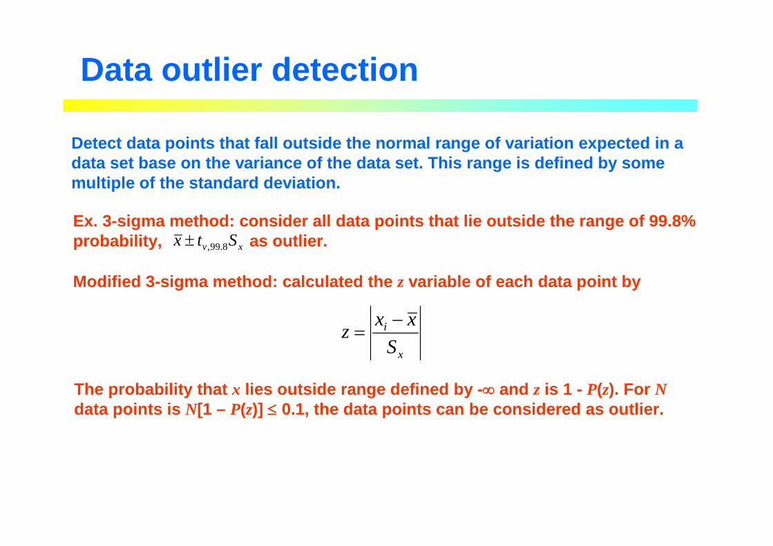
Data outlier detection

Detect data points that fall outside the normal ran ge of variation expected in a data set base on the variance of the data set. This range is defined by some multiple of the standard deviation.

Ex. 3-sigma method: consider all data points that l ie outside the range of 99.8% probability, as outlier. 8.99, xv Stx ±

Modified 3-sigma method: calculated the z variable of each data point by

x

i

S

xxz

−=

The probability that x lies outside range defined by - ∞∞∞∞ and z is 1 - P(z). For Ndata points is N[1 – P(z)] ≤≤≤≤ 0.1, the data points can be considered as outlier.

Example: Consider the data given here for 10 measurements of tire pressure taken with an inexpensive handheld gauge. Compute the statistics of the data set; then test for outlier by using the modified three-sigma test

Known: N = 10

Solution:

Assume: Each measurement obtained under fixed condi tions

Data outlier detection

n i x [psi] |z| P (|z|) N(1-P(|z|)

1 28 0.3 0.6199 3.80102 31 1.1 0.8724 1.27643 27 0.0 0.5111 4.88934 28 0.3 0.6199 3.80105 29 0.6 0.7199 2.80056 24 0.8 0.7895 2.10517 29 0.6 0.7199 2.80058 28 0.3 0.6199 3.80109 18 2.5 0.9932 0.067710 27 0.0 0.5111 4.8893

N = 10: x = 27, Sx = 3.604

N = 9: x = 28, Sx = 2.0, t8,95 = 2.306

(95%) psi 6.128 , ±=±=N

Stx xPvµ

After removing the spurious data

Statistics at start

Number of Measurement

The precision interval is two sided about sample me an that true mean to be within. to . Here, we define the one-side precision value d as

/, NSt xPv− /, NSt xPv+

N

Std xv,P =

The required number of measurement is estimated by

%

2

Pd

StN xv,P

≈

The estimated of sample variance is needed. If we d o a preliminary small number of measurements, N1 for estimate sample variance, S1. The total number of measurements, NT will be

%

2

111 Pd

StN ,PN

T

≈ −

NT – N1 additional measurements will be required.

Example: Determine the number of measurements required to reduce the confidential interval of the mean value of a variable to within 1 unit if the variance of the variable is estimated to be ~64 units.Known: P = 95% d = ½ σσσσ2 = 64 units

N = 983Solution:

Assume: σσσσ2 ≈≈≈≈ S2x

Number of Measurement

5%9

2

≈

d

StN xv,P

The regression analysis for a single variable of th e form y = f(x) provides an mth order polynomial fit of the data in the form. varia ble

Least-Square Regression Analysis

Where yc is the value of the dependent variable obtained dir ectly from the polynomial equation for a given value of x. For N different values of independent and dependent value included in the ana lysis, the highest order, m, of the polynomial that can be determined is restric ted to m ≤≤≤≤ N – 1.

The values of the m + 1 coefficients a0, a1, …, am are determined by the least square method. The least-squares technique attempts to minimize the sum of the square of the deviations between the actual dat a and the polynomial fit

mmc xaxaxaay ++++= ...2

210

∑=

−=N

ici yyD

1

2)(Minimize

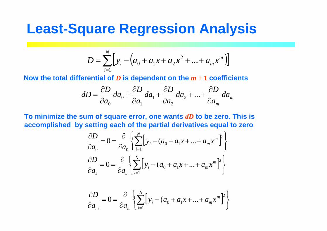
Least-Square Regression Analysis

( )[ ]∑=

++++−=N

i

mmi xaxaxaayD

1

2210 ...

To minimize the sum of square error, one wants dD to be zero. This is accomplished by setting each of the partial deriva tives equal to zero

Now the total differential of D is dependent on the m + 1 coefficients

mm

daa

Dda

a

Dda

a

Dda

a

DdD

∂∂

++∂∂

+∂∂

+∂∂

= ...22

11

00

[ ]

[ ]

[ ]

+++−∂∂

==∂∂

+++−∂∂

==∂∂

+++−∂∂

==∂∂

∑

∑

∑

=

=

=

N

i

mmi

mm

N

i

mmi

N

i

mmi

xaxaayaa

D

xaxaayaa

D

xaxaayaa

D

1

2

10

1

2

1011

1

2

1000

...(0

...(0

...(0

Least-Square Regression Analysis

This yields m + 1 equations, which are solved simultaneously to yield the unknown regression coefficients, a0, a1, …, am

v

yyS

N

ici

yx

∑=

−= 1

2)(

Standard deviation based on the deviation of the ea ch data point and the fit by

A measure of the precision

We can state that the curve fit with its precision interval as

%)( , PSty yxPvc ±

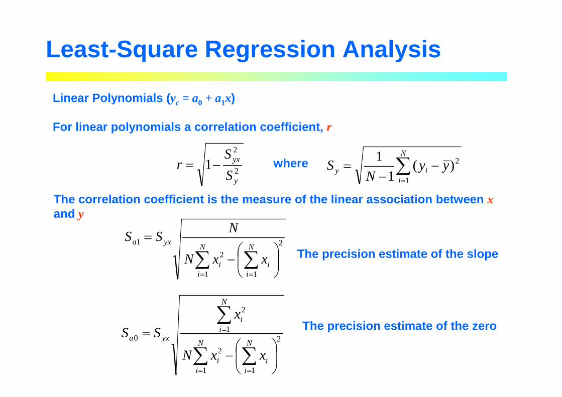
Least-Square Regression Analysis

where

2

11

2

1

−

=

∑∑==

N

ii

N

ii

yxa

xxN

NSS

The correlation coefficient is the measure of the l inear association between x and y

The precision estimate of the slope

Linear Polynomials ( yc = a0 + a1x)

For linear polynomials a correlation coefficient, r

2

2

1y

yx

S

Sr −= ∑

=

−−

=N

iiy yy

NS

1

2)(1

1

2

11

2

1

2

0

−

=

∑∑

∑

==

=

N

ii

N

ii

N

ii

yxa

xxN

xSS The precision estimate of the zero

Least-Square Regression Analysis

Example: The following data are suspected to follow a linear relationship. Find an appropriate equation of the first-order form

Known: Independent variable, xDependent variable, yN = 5

Solution:

Assume: Linear relation

x [cm] y [V]1 1.22 1.93 3.24 4.15 5.3

yc = a0 + a1x

x[cm] y[V] x 2 y2 xy1 1.2 1 1.44 1.22 1.9 4 3.61 3.83 3.2 9 10.24 9.64 4.1 16 16.81 16.45 5.3 25 28.09 26.5

ΣΣΣΣ 15 15.7 55 60.19 57.5

yc = 0.02 + 1.04x

νννν = N - (m+1) = 5 - (1+1) = 3