Probabilistic Wind Turbine System Models in Three Courses ... · Probabilistic Wind Turbine System...
25
Probabilistic Wind Turbine System Models in Three Courses: Composite Materials, Aerodynamics, Grid Integration Dr. Curran Crawford Department of Mechanical Engineering University of Victoria 4th Workshop on Systems Engineering for Wind Energy DTU Vindenergi, September 13, 2017 1/ 26
Transcript of Probabilistic Wind Turbine System Models in Three Courses ... · Probabilistic Wind Turbine System...

Probabilistic Wind Turbine System Models in Three Courses Composite Materials
Aerodynamics Grid Integration
Dr Curran Crawford
Department of Mechanical Engineering University of Victoria
4th Workshop on Systems Engineering for Wind Energy DTU Vindenergi September 13 2017
1 26
Outline
Why Probabilistic Models
Composite Structures
Turbulent Aero(structural) dynamics
(Smart) Grid Integration
2 26
Table of Contents
Why Probabilistic Models
Composite Structures
Turbulent Aero(structural) dynamics
(Smart) Grid Integration
3 26
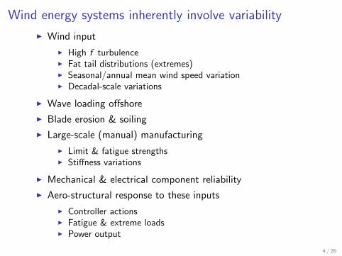
Wind energy systems inherently involve variability
Wind input
High f turbulence Fat tail distributions (extremes) Seasonalannual mean wind speed variation Decadal-scale variations
Wave loading offshore
Blade erosion amp soiling
Large-scale (manual) manufacturing
Limit amp fatigue strengths Stiffness variations
Mechanical amp electrical component reliability
Aero-structural response to these inputs
Controller actions Fatigue amp extreme loads Power output
4 26
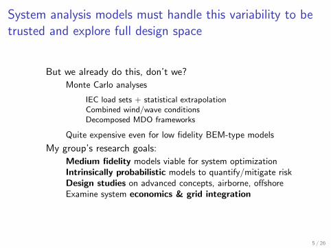
System analysis models must handle this variability to be trusted and explore full design space
But we already do this donrsquot we Monte Carlo analyses
IEC load sets + statistical extrapolation Combined windwave conditions Decomposed MDO frameworks
Quite expensive even for low fidelity BEM-type models
My grouprsquos research goals Medium fidelity models viable for system optimization Intrinsically probabilistic models to quantifymitigate risk Design studies on advanced concepts airborne offshore Examine system economics amp grid integration
5 26
Table of Contents
Why Probabilistic Models
Composite Structures
Turbulent Aero(structural) dynamics
(Smart) Grid Integration
6 26
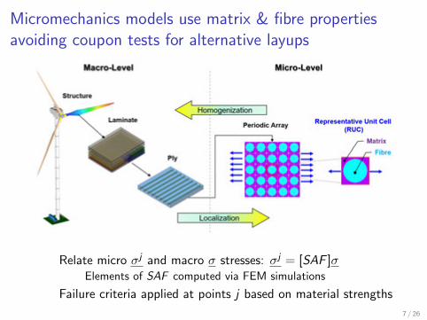
Micromechanics models use matrix amp fibre properties avoiding coupon tests for alternative layups
Relate micro σj and macro σ stresses σj = [SAF ]σ Elements of SAF computed via FEM simulations
Failure criteria applied at points j based on material strengths
7 26
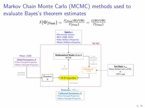
Markov Chain Monte Carlo (MCMC) methods used to evaluate Bayesrsquos theorem estimates
f (ytest |Θ)f (Θ) L(Θ)f (Θ)f (Θ|ytest ) = = f (ytest ) f (ytest )
8 26
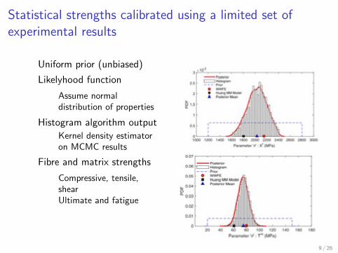
Statistical strengths calibrated using a limited set of experimental results
Uniform prior (unbiased)
Likelyhood function
Assume normal distribution of properties
Histogram algorithm output Kernel density estimator on MCMC results
Fibre and matrix strengths
Compressive tensile shear Ultimate and fatigue
9 26
Forward statistical analysis of candidate layups is then possible (ultimate amp fatigue)
10 26
Table of Contents
Why Probabilistic Models
Composite Structures
Turbulent Aero(structural) dynamics
(Smart) Grid Integration
11 26
To explore new (multi-MW scale floating) concepts need to get beyond BEM
Physics not captured by BEM
Non-linear motion amp deflections Sweptwinglet blades
Unsteady aerodynamics
CFD still to costly for unsteady design
Vortex-based methods appropriate
But costly for unsteady design
Also want gradients for unsteady performance
12 26
stochastic input process solve system
equations
several realizations(only if needed)
analyze results
Γξ i(t)=f (uξ i(t))
Γ(t ξ)=f (u(t ξ))
several realizations
one stochastic solution
several deterministic solutions
Fundamentally we want to replace many time-domain simulations with a single solution in the stochastic space
13 26
We have adopted intrusive chaos (polynomial) methods to analyze in the stochastic domain
Expand wind inflow model with random phase angles ξ isin [minusπ π] as
Rminus1R uinfin(tn ξ) = ur (tn)Ψr (ξ)
r=0
Lots of groundwork on describing correlated wind fields with minimum number of ξ phase angles Expand circulate strength Γ (lift) as
Rminus1R Γ(tn ξ) = gr (tn)Ψr (ξ)
r =0
Functionals Ψr (ξ) define polynomials (exponentials) of random variable ξ
Choose form based on PDF of ξ Legendre polynomials for uniform distributions
14 26
Solution procedure is equivalent to one time-domain solve but obtain results for all possible ξ values
Use inner product (D Ψr (ξ)) lsquostochastic Galerkinrsquo projection
Orthogonality property of Ψr (ξ) when chosen correctly Equations for coefficients in time fall out
ur (tn) gr (tn)
Note that these solutions are functions of time
Not a Fourier transform Can handle non-linear time dependent effects
Output quantity calculations
Time-domain for specific ξ realization
Validation with time dependent code
Directly compute statistical moments from gr (tn) PDF reconstruction methods
All possible wind input fields evaluated simultaneously
15 26
Wersquove applied the stochastic Galerkin method to stationary bladeswings (lifting line)
tra
iling
fila
men
ts
Γ j(k
+1
)
k =
1
k =
M
i = N
+1
j= N
j= 1
i = 1
c)
xx
xx
x
r ijk
Γikshed
elements
x
x xxx
xxx x x x
x
xx
xx
xx
xxx
xxx
xX
ik
X(i+
1)k
x
x xxx
x
y
γ20
γ10
γ50 γN b N t
γ12Γ1(t n)
Γ2(t n)
Γ3(tn)
Γ4(tn)
Γ5(tn)
Γs 11
Γs 21
Γs 42H 3(s 51)
G3(s 23)
Γt 13
Γt 51
Nt elements
Nb e
lem
ents
γ31
16 26
Wersquove applied the stochastic Galerkin method to stationary bladeswings (lifting line)
span position [m]-25 -15 -5 5 15 25
circula
tion [m
2s
]
5
10
15
steady state stochastic at t=[68101214] s
wind speed [ms]8 10 12 8 10 12 8 10 12 8 10 12 8 10 12 8 10 12
tim
e [s]
0
5
10
15
wind bound circulation (deterministic) bound circulation (stochstic)
circulation [m2s]
9 11 13 9 11 13 9 11 13 9 11 13 9 11 13 9 11 13
17 26
and simplified BEM compared to 100 deterministic sample wind inputs
3 6 9 12 15 18
time [s]
0
10
20
30
element at rR=014
element at rR=086
18 26
Table of Contents
Why Probabilistic Models
Composite Structures
Turbulent Aero(structural) dynamics
(Smart) Grid Integration
19 26
Wind energyrsquos value depends on the grid-delivered product hopefully greater than the costs to provide it
Various components in levelized cost of energy Base materials ndash capital costs Aerostructural performance ndash power captureloads Variability in system costs captured with previous approaches
But value is different than costs Levelized avoided cost of energy (LACE)
LCOE estimates revenue requirements LACE estimates revenues available
Firming services costs
How to model variable grid system performance
20 26
The interconnected grid is large and complicated requiring efficient solutions methods
BPAT
BCHAAESO
WAUWNWMT
IPCO
AVA
PGE
PACW
PACE
WACM
PSCO
PNM
EPE
WALC
SRP
AZPS
IID
PSEISCL
TPWR
DOPDCHPD
DEAAGRMA
HGMATEPC
LDWP
BANC
TIDC
CFE
CISO
GCPDWWA
GRIF
GWA
NEVP
GRID
Boundaries are approximate and for illustrative purposes only
Western InterconnectionBalancing Authorities (38)
AESO - Alberta Electric System OperatorAZPS - Arizona Public Service CompanyAVA - Avista CorporationBANC - Balancing Authority of Northern CaliforniaBPAT - Bonneville Power Administration - TransmissionBCHA - British Columbia Hydro AuthorityCISO - California Independent System OperatorCFE - Comision Federal de ElectricidadDEAA - Arlington Valley LLCEPE - El Paso Electric CompanyGRMA - Gila River Power LPGRID - GridforceGRIF - Grith Energy LLCIPCO - Idaho Power Company
IID - Imperial Irrigation DistrictLDWP - Los Angeles Department of Water and PowerGWA - NaturEner Power Watch LLCNEVP - Nevada Power CompanyHGMA - New Harquahala Generating Company LLCNWMT - NorthWestern EnergyPACE - PaciCorp EastPACW - PaciCorp WestPGE - Portland General Electric CompanyPSCO - Public Service Company of ColoradoPNM - Public Service Company of New MexicoCHPD - PUD No 1 of Chelan CountyDOPD - PUD No 1 of Douglas CountyGCPD - PUD No 2 of Grant County
PSEI - Puget Sound EnergySRP - Salt River ProjectSCL - Seattle City LightTPWR - City of Tacoma Department of Public Utilities TEPC - Tucson Electric Power CompanyTIDC - Turlock Irrigation DistrictWACM - Western Area Power Administration Colorado-Missouri RegionWALC - Western Area Power Administration Lower Colorado RegionWAUW - Western Area Power Administration Upper Great Plains WestWWA - NaturEner Wind Watch LLC
011915hr
21 26
The power grid is modeled by a set of (non-)linear power flow equations
Distribution and transmission grid governing equations
[Pi Qi ] = f (Vi δi ) [Pik Qik ] = f (Vi Vk δik )
22 26
Cumulant-based analysis methods to handle stochastic generation and loads on each bus
Input definition Real Pi and imaginary Qi power injections represent generation and loads on each bus
Compute moments microv of the distributions Convert moments to cumulants κv of those distributions
Analysis method
Basic cumulant arithmetic for Y = AX κY v = Av κX v
We extended to cumulant tensors for correlated variables and polynomial functionals
Linearize polar form of equations amp truncate Rectangular form of power flow equation expansion rArr exact quadratic equation
Post-process results
[Vi δi Pik Qik ] outputs impacting costs etc Maximum-entropy PDF reconstruction from κv
23 26
IEEE 14 bus example with wind power generation and plug-in vehicle loads
24 26
Thanks for listening
Dr Curran Crawford
E-mail currancuvicca
Website wwwssdluvicca
Twitter SSDLab
Students
Composites Ghulam Mustafa
Aero Manuel Fluck Rad Haghi
Grid Trevor Williams Pouya Amid
25 26
- Why Probabilistic Models
- Composite Structures
- Turbulent Aero(structural) dynamics
- (Smart) Grid Integration
-
Outline
Why Probabilistic Models
Composite Structures
Turbulent Aero(structural) dynamics
(Smart) Grid Integration
2 26
Table of Contents
Why Probabilistic Models
Composite Structures
Turbulent Aero(structural) dynamics
(Smart) Grid Integration
3 26
Wind energy systems inherently involve variability
Wind input
High f turbulence Fat tail distributions (extremes) Seasonalannual mean wind speed variation Decadal-scale variations
Wave loading offshore
Blade erosion amp soiling
Large-scale (manual) manufacturing
Limit amp fatigue strengths Stiffness variations
Mechanical amp electrical component reliability
Aero-structural response to these inputs
Controller actions Fatigue amp extreme loads Power output
4 26
System analysis models must handle this variability to be trusted and explore full design space
But we already do this donrsquot we Monte Carlo analyses
IEC load sets + statistical extrapolation Combined windwave conditions Decomposed MDO frameworks
Quite expensive even for low fidelity BEM-type models
My grouprsquos research goals Medium fidelity models viable for system optimization Intrinsically probabilistic models to quantifymitigate risk Design studies on advanced concepts airborne offshore Examine system economics amp grid integration
5 26
Table of Contents
Why Probabilistic Models
Composite Structures
Turbulent Aero(structural) dynamics
(Smart) Grid Integration
6 26
Micromechanics models use matrix amp fibre properties avoiding coupon tests for alternative layups
Relate micro σj and macro σ stresses σj = [SAF ]σ Elements of SAF computed via FEM simulations
Failure criteria applied at points j based on material strengths
7 26
Markov Chain Monte Carlo (MCMC) methods used to evaluate Bayesrsquos theorem estimates
f (ytest |Θ)f (Θ) L(Θ)f (Θ)f (Θ|ytest ) = = f (ytest ) f (ytest )
8 26
Statistical strengths calibrated using a limited set of experimental results
Uniform prior (unbiased)
Likelyhood function
Assume normal distribution of properties
Histogram algorithm output Kernel density estimator on MCMC results
Fibre and matrix strengths
Compressive tensile shear Ultimate and fatigue
9 26
Forward statistical analysis of candidate layups is then possible (ultimate amp fatigue)
10 26
Table of Contents
Why Probabilistic Models
Composite Structures
Turbulent Aero(structural) dynamics
(Smart) Grid Integration
11 26
To explore new (multi-MW scale floating) concepts need to get beyond BEM
Physics not captured by BEM
Non-linear motion amp deflections Sweptwinglet blades
Unsteady aerodynamics
CFD still to costly for unsteady design
Vortex-based methods appropriate
But costly for unsteady design
Also want gradients for unsteady performance
12 26
stochastic input process solve system
equations
several realizations(only if needed)
analyze results
Γξ i(t)=f (uξ i(t))
Γ(t ξ)=f (u(t ξ))
several realizations
one stochastic solution
several deterministic solutions
Fundamentally we want to replace many time-domain simulations with a single solution in the stochastic space
13 26
We have adopted intrusive chaos (polynomial) methods to analyze in the stochastic domain
Expand wind inflow model with random phase angles ξ isin [minusπ π] as
Rminus1R uinfin(tn ξ) = ur (tn)Ψr (ξ)
r=0
Lots of groundwork on describing correlated wind fields with minimum number of ξ phase angles Expand circulate strength Γ (lift) as
Rminus1R Γ(tn ξ) = gr (tn)Ψr (ξ)
r =0
Functionals Ψr (ξ) define polynomials (exponentials) of random variable ξ
Choose form based on PDF of ξ Legendre polynomials for uniform distributions
14 26
Solution procedure is equivalent to one time-domain solve but obtain results for all possible ξ values
Use inner product (D Ψr (ξ)) lsquostochastic Galerkinrsquo projection
Orthogonality property of Ψr (ξ) when chosen correctly Equations for coefficients in time fall out
ur (tn) gr (tn)
Note that these solutions are functions of time
Not a Fourier transform Can handle non-linear time dependent effects
Output quantity calculations
Time-domain for specific ξ realization
Validation with time dependent code
Directly compute statistical moments from gr (tn) PDF reconstruction methods
All possible wind input fields evaluated simultaneously
15 26
Wersquove applied the stochastic Galerkin method to stationary bladeswings (lifting line)
tra
iling
fila
men
ts
Γ j(k
+1
)
k =
1
k =
M
i = N
+1
j= N
j= 1
i = 1
c)
xx
xx
x
r ijk
Γikshed
elements
x
x xxx
xxx x x x
x
xx
xx
xx
xxx
xxx
xX
ik
X(i+
1)k
x
x xxx
x
y
γ20
γ10
γ50 γN b N t
γ12Γ1(t n)
Γ2(t n)
Γ3(tn)
Γ4(tn)
Γ5(tn)
Γs 11
Γs 21
Γs 42H 3(s 51)
G3(s 23)
Γt 13
Γt 51
Nt elements
Nb e
lem
ents
γ31
16 26
Wersquove applied the stochastic Galerkin method to stationary bladeswings (lifting line)
span position [m]-25 -15 -5 5 15 25
circula
tion [m
2s
]
5
10
15
steady state stochastic at t=[68101214] s
wind speed [ms]8 10 12 8 10 12 8 10 12 8 10 12 8 10 12 8 10 12
tim
e [s]
0
5
10
15
wind bound circulation (deterministic) bound circulation (stochstic)
circulation [m2s]
9 11 13 9 11 13 9 11 13 9 11 13 9 11 13 9 11 13
17 26
and simplified BEM compared to 100 deterministic sample wind inputs
3 6 9 12 15 18
time [s]
0
10
20
30
element at rR=014
element at rR=086
18 26
Table of Contents
Why Probabilistic Models
Composite Structures
Turbulent Aero(structural) dynamics
(Smart) Grid Integration
19 26
Wind energyrsquos value depends on the grid-delivered product hopefully greater than the costs to provide it
Various components in levelized cost of energy Base materials ndash capital costs Aerostructural performance ndash power captureloads Variability in system costs captured with previous approaches
But value is different than costs Levelized avoided cost of energy (LACE)
LCOE estimates revenue requirements LACE estimates revenues available
Firming services costs
How to model variable grid system performance
20 26
The interconnected grid is large and complicated requiring efficient solutions methods
BPAT
BCHAAESO
WAUWNWMT
IPCO
AVA
PGE
PACW
PACE
WACM
PSCO
PNM
EPE
WALC
SRP
AZPS
IID
PSEISCL
TPWR
DOPDCHPD
DEAAGRMA
HGMATEPC
LDWP
BANC
TIDC
CFE
CISO
GCPDWWA
GRIF
GWA
NEVP
GRID
Boundaries are approximate and for illustrative purposes only
Western InterconnectionBalancing Authorities (38)
AESO - Alberta Electric System OperatorAZPS - Arizona Public Service CompanyAVA - Avista CorporationBANC - Balancing Authority of Northern CaliforniaBPAT - Bonneville Power Administration - TransmissionBCHA - British Columbia Hydro AuthorityCISO - California Independent System OperatorCFE - Comision Federal de ElectricidadDEAA - Arlington Valley LLCEPE - El Paso Electric CompanyGRMA - Gila River Power LPGRID - GridforceGRIF - Grith Energy LLCIPCO - Idaho Power Company
IID - Imperial Irrigation DistrictLDWP - Los Angeles Department of Water and PowerGWA - NaturEner Power Watch LLCNEVP - Nevada Power CompanyHGMA - New Harquahala Generating Company LLCNWMT - NorthWestern EnergyPACE - PaciCorp EastPACW - PaciCorp WestPGE - Portland General Electric CompanyPSCO - Public Service Company of ColoradoPNM - Public Service Company of New MexicoCHPD - PUD No 1 of Chelan CountyDOPD - PUD No 1 of Douglas CountyGCPD - PUD No 2 of Grant County
PSEI - Puget Sound EnergySRP - Salt River ProjectSCL - Seattle City LightTPWR - City of Tacoma Department of Public Utilities TEPC - Tucson Electric Power CompanyTIDC - Turlock Irrigation DistrictWACM - Western Area Power Administration Colorado-Missouri RegionWALC - Western Area Power Administration Lower Colorado RegionWAUW - Western Area Power Administration Upper Great Plains WestWWA - NaturEner Wind Watch LLC
011915hr
21 26
The power grid is modeled by a set of (non-)linear power flow equations
Distribution and transmission grid governing equations
[Pi Qi ] = f (Vi δi ) [Pik Qik ] = f (Vi Vk δik )
22 26
Cumulant-based analysis methods to handle stochastic generation and loads on each bus
Input definition Real Pi and imaginary Qi power injections represent generation and loads on each bus
Compute moments microv of the distributions Convert moments to cumulants κv of those distributions
Analysis method
Basic cumulant arithmetic for Y = AX κY v = Av κX v
We extended to cumulant tensors for correlated variables and polynomial functionals
Linearize polar form of equations amp truncate Rectangular form of power flow equation expansion rArr exact quadratic equation
Post-process results
[Vi δi Pik Qik ] outputs impacting costs etc Maximum-entropy PDF reconstruction from κv
23 26
IEEE 14 bus example with wind power generation and plug-in vehicle loads
24 26
Thanks for listening
Dr Curran Crawford
E-mail currancuvicca
Website wwwssdluvicca
Twitter SSDLab
Students
Composites Ghulam Mustafa
Aero Manuel Fluck Rad Haghi
Grid Trevor Williams Pouya Amid
25 26
- Why Probabilistic Models
- Composite Structures
- Turbulent Aero(structural) dynamics
- (Smart) Grid Integration
-
Table of Contents
Why Probabilistic Models
Composite Structures
Turbulent Aero(structural) dynamics
(Smart) Grid Integration
3 26
Wind energy systems inherently involve variability
Wind input
High f turbulence Fat tail distributions (extremes) Seasonalannual mean wind speed variation Decadal-scale variations
Wave loading offshore
Blade erosion amp soiling
Large-scale (manual) manufacturing
Limit amp fatigue strengths Stiffness variations
Mechanical amp electrical component reliability
Aero-structural response to these inputs
Controller actions Fatigue amp extreme loads Power output
4 26
System analysis models must handle this variability to be trusted and explore full design space
But we already do this donrsquot we Monte Carlo analyses
IEC load sets + statistical extrapolation Combined windwave conditions Decomposed MDO frameworks
Quite expensive even for low fidelity BEM-type models
My grouprsquos research goals Medium fidelity models viable for system optimization Intrinsically probabilistic models to quantifymitigate risk Design studies on advanced concepts airborne offshore Examine system economics amp grid integration
5 26
Table of Contents
Why Probabilistic Models
Composite Structures
Turbulent Aero(structural) dynamics
(Smart) Grid Integration
6 26
Micromechanics models use matrix amp fibre properties avoiding coupon tests for alternative layups
Relate micro σj and macro σ stresses σj = [SAF ]σ Elements of SAF computed via FEM simulations
Failure criteria applied at points j based on material strengths
7 26
Markov Chain Monte Carlo (MCMC) methods used to evaluate Bayesrsquos theorem estimates
f (ytest |Θ)f (Θ) L(Θ)f (Θ)f (Θ|ytest ) = = f (ytest ) f (ytest )
8 26
Statistical strengths calibrated using a limited set of experimental results
Uniform prior (unbiased)
Likelyhood function
Assume normal distribution of properties
Histogram algorithm output Kernel density estimator on MCMC results
Fibre and matrix strengths
Compressive tensile shear Ultimate and fatigue
9 26
Forward statistical analysis of candidate layups is then possible (ultimate amp fatigue)
10 26
Table of Contents
Why Probabilistic Models
Composite Structures
Turbulent Aero(structural) dynamics
(Smart) Grid Integration
11 26
To explore new (multi-MW scale floating) concepts need to get beyond BEM
Physics not captured by BEM
Non-linear motion amp deflections Sweptwinglet blades
Unsteady aerodynamics
CFD still to costly for unsteady design
Vortex-based methods appropriate
But costly for unsteady design
Also want gradients for unsteady performance
12 26
stochastic input process solve system
equations
several realizations(only if needed)
analyze results
Γξ i(t)=f (uξ i(t))
Γ(t ξ)=f (u(t ξ))
several realizations
one stochastic solution
several deterministic solutions
Fundamentally we want to replace many time-domain simulations with a single solution in the stochastic space
13 26
We have adopted intrusive chaos (polynomial) methods to analyze in the stochastic domain
Expand wind inflow model with random phase angles ξ isin [minusπ π] as
Rminus1R uinfin(tn ξ) = ur (tn)Ψr (ξ)
r=0
Lots of groundwork on describing correlated wind fields with minimum number of ξ phase angles Expand circulate strength Γ (lift) as
Rminus1R Γ(tn ξ) = gr (tn)Ψr (ξ)
r =0
Functionals Ψr (ξ) define polynomials (exponentials) of random variable ξ
Choose form based on PDF of ξ Legendre polynomials for uniform distributions
14 26
Solution procedure is equivalent to one time-domain solve but obtain results for all possible ξ values
Use inner product (D Ψr (ξ)) lsquostochastic Galerkinrsquo projection
Orthogonality property of Ψr (ξ) when chosen correctly Equations for coefficients in time fall out
ur (tn) gr (tn)
Note that these solutions are functions of time
Not a Fourier transform Can handle non-linear time dependent effects
Output quantity calculations
Time-domain for specific ξ realization
Validation with time dependent code
Directly compute statistical moments from gr (tn) PDF reconstruction methods
All possible wind input fields evaluated simultaneously
15 26
Wersquove applied the stochastic Galerkin method to stationary bladeswings (lifting line)
tra
iling
fila
men
ts
Γ j(k
+1
)
k =
1
k =
M
i = N
+1
j= N
j= 1
i = 1
c)
xx
xx
x
r ijk
Γikshed
elements
x
x xxx
xxx x x x
x
xx
xx
xx
xxx
xxx
xX
ik
X(i+
1)k
x
x xxx
x
y
γ20
γ10
γ50 γN b N t
γ12Γ1(t n)
Γ2(t n)
Γ3(tn)
Γ4(tn)
Γ5(tn)
Γs 11
Γs 21
Γs 42H 3(s 51)
G3(s 23)
Γt 13
Γt 51
Nt elements
Nb e
lem
ents
γ31
16 26
Wersquove applied the stochastic Galerkin method to stationary bladeswings (lifting line)
span position [m]-25 -15 -5 5 15 25
circula
tion [m
2s
]
5
10
15
steady state stochastic at t=[68101214] s
wind speed [ms]8 10 12 8 10 12 8 10 12 8 10 12 8 10 12 8 10 12
tim
e [s]
0
5
10
15
wind bound circulation (deterministic) bound circulation (stochstic)
circulation [m2s]
9 11 13 9 11 13 9 11 13 9 11 13 9 11 13 9 11 13
17 26
and simplified BEM compared to 100 deterministic sample wind inputs
3 6 9 12 15 18
time [s]
0
10
20
30
element at rR=014
element at rR=086
18 26
Table of Contents
Why Probabilistic Models
Composite Structures
Turbulent Aero(structural) dynamics
(Smart) Grid Integration
19 26
Wind energyrsquos value depends on the grid-delivered product hopefully greater than the costs to provide it
Various components in levelized cost of energy Base materials ndash capital costs Aerostructural performance ndash power captureloads Variability in system costs captured with previous approaches
But value is different than costs Levelized avoided cost of energy (LACE)
LCOE estimates revenue requirements LACE estimates revenues available
Firming services costs
How to model variable grid system performance
20 26
The interconnected grid is large and complicated requiring efficient solutions methods
BPAT
BCHAAESO
WAUWNWMT
IPCO
AVA
PGE
PACW
PACE
WACM
PSCO
PNM
EPE
WALC
SRP
AZPS
IID
PSEISCL
TPWR
DOPDCHPD
DEAAGRMA
HGMATEPC
LDWP
BANC
TIDC
CFE
CISO
GCPDWWA
GRIF
GWA
NEVP
GRID
Boundaries are approximate and for illustrative purposes only
Western InterconnectionBalancing Authorities (38)
AESO - Alberta Electric System OperatorAZPS - Arizona Public Service CompanyAVA - Avista CorporationBANC - Balancing Authority of Northern CaliforniaBPAT - Bonneville Power Administration - TransmissionBCHA - British Columbia Hydro AuthorityCISO - California Independent System OperatorCFE - Comision Federal de ElectricidadDEAA - Arlington Valley LLCEPE - El Paso Electric CompanyGRMA - Gila River Power LPGRID - GridforceGRIF - Grith Energy LLCIPCO - Idaho Power Company
IID - Imperial Irrigation DistrictLDWP - Los Angeles Department of Water and PowerGWA - NaturEner Power Watch LLCNEVP - Nevada Power CompanyHGMA - New Harquahala Generating Company LLCNWMT - NorthWestern EnergyPACE - PaciCorp EastPACW - PaciCorp WestPGE - Portland General Electric CompanyPSCO - Public Service Company of ColoradoPNM - Public Service Company of New MexicoCHPD - PUD No 1 of Chelan CountyDOPD - PUD No 1 of Douglas CountyGCPD - PUD No 2 of Grant County
PSEI - Puget Sound EnergySRP - Salt River ProjectSCL - Seattle City LightTPWR - City of Tacoma Department of Public Utilities TEPC - Tucson Electric Power CompanyTIDC - Turlock Irrigation DistrictWACM - Western Area Power Administration Colorado-Missouri RegionWALC - Western Area Power Administration Lower Colorado RegionWAUW - Western Area Power Administration Upper Great Plains WestWWA - NaturEner Wind Watch LLC
011915hr
21 26
The power grid is modeled by a set of (non-)linear power flow equations
Distribution and transmission grid governing equations
[Pi Qi ] = f (Vi δi ) [Pik Qik ] = f (Vi Vk δik )
22 26
Cumulant-based analysis methods to handle stochastic generation and loads on each bus
Input definition Real Pi and imaginary Qi power injections represent generation and loads on each bus
Compute moments microv of the distributions Convert moments to cumulants κv of those distributions
Analysis method
Basic cumulant arithmetic for Y = AX κY v = Av κX v
We extended to cumulant tensors for correlated variables and polynomial functionals
Linearize polar form of equations amp truncate Rectangular form of power flow equation expansion rArr exact quadratic equation
Post-process results
[Vi δi Pik Qik ] outputs impacting costs etc Maximum-entropy PDF reconstruction from κv
23 26
IEEE 14 bus example with wind power generation and plug-in vehicle loads
24 26
Thanks for listening
Dr Curran Crawford
E-mail currancuvicca
Website wwwssdluvicca
Twitter SSDLab
Students
Composites Ghulam Mustafa
Aero Manuel Fluck Rad Haghi
Grid Trevor Williams Pouya Amid
25 26
- Why Probabilistic Models
- Composite Structures
- Turbulent Aero(structural) dynamics
- (Smart) Grid Integration
-
Table of Contents
Why Probabilistic Models
Composite Structures
Turbulent Aero(structural) dynamics
(Smart) Grid Integration
6 26
Micromechanics models use matrix amp fibre properties avoiding coupon tests for alternative layups
Relate micro σj and macro σ stresses σj = [SAF ]σ Elements of SAF computed via FEM simulations
Failure criteria applied at points j based on material strengths
7 26
Markov Chain Monte Carlo (MCMC) methods used to evaluate Bayesrsquos theorem estimates
f (ytest |Θ)f (Θ) L(Θ)f (Θ)f (Θ|ytest ) = = f (ytest ) f (ytest )
8 26
Statistical strengths calibrated using a limited set of experimental results
Uniform prior (unbiased)
Likelyhood function
Assume normal distribution of properties
Histogram algorithm output Kernel density estimator on MCMC results
Fibre and matrix strengths
Compressive tensile shear Ultimate and fatigue
9 26
Forward statistical analysis of candidate layups is then possible (ultimate amp fatigue)
10 26
Table of Contents
Why Probabilistic Models
Composite Structures
Turbulent Aero(structural) dynamics
(Smart) Grid Integration
11 26
To explore new (multi-MW scale floating) concepts need to get beyond BEM
Physics not captured by BEM
Non-linear motion amp deflections Sweptwinglet blades
Unsteady aerodynamics
CFD still to costly for unsteady design
Vortex-based methods appropriate
But costly for unsteady design
Also want gradients for unsteady performance
12 26
stochastic input process solve system
equations
several realizations(only if needed)
analyze results
Γξ i(t)=f (uξ i(t))
Γ(t ξ)=f (u(t ξ))
several realizations
one stochastic solution
several deterministic solutions
Fundamentally we want to replace many time-domain simulations with a single solution in the stochastic space
13 26
We have adopted intrusive chaos (polynomial) methods to analyze in the stochastic domain
Expand wind inflow model with random phase angles ξ isin [minusπ π] as
Rminus1R uinfin(tn ξ) = ur (tn)Ψr (ξ)
r=0
Lots of groundwork on describing correlated wind fields with minimum number of ξ phase angles Expand circulate strength Γ (lift) as
Rminus1R Γ(tn ξ) = gr (tn)Ψr (ξ)
r =0
Functionals Ψr (ξ) define polynomials (exponentials) of random variable ξ
Choose form based on PDF of ξ Legendre polynomials for uniform distributions
14 26
Solution procedure is equivalent to one time-domain solve but obtain results for all possible ξ values
Use inner product (D Ψr (ξ)) lsquostochastic Galerkinrsquo projection
Orthogonality property of Ψr (ξ) when chosen correctly Equations for coefficients in time fall out
ur (tn) gr (tn)
Note that these solutions are functions of time
Not a Fourier transform Can handle non-linear time dependent effects
Output quantity calculations
Time-domain for specific ξ realization
Validation with time dependent code
Directly compute statistical moments from gr (tn) PDF reconstruction methods
All possible wind input fields evaluated simultaneously
15 26
Wersquove applied the stochastic Galerkin method to stationary bladeswings (lifting line)
tra
iling
fila
men
ts
Γ j(k
+1
)
k =
1
k =
M
i = N
+1
j= N
j= 1
i = 1
c)
xx
xx
x
r ijk
Γikshed
elements
x
x xxx
xxx x x x
x
xx
xx
xx
xxx
xxx
xX
ik
X(i+
1)k
x
x xxx
x
y
γ20
γ10
γ50 γN b N t
γ12Γ1(t n)
Γ2(t n)
Γ3(tn)
Γ4(tn)
Γ5(tn)
Γs 11
Γs 21
Γs 42H 3(s 51)
G3(s 23)
Γt 13
Γt 51
Nt elements
Nb e
lem
ents
γ31
16 26
Wersquove applied the stochastic Galerkin method to stationary bladeswings (lifting line)
span position [m]-25 -15 -5 5 15 25
circula
tion [m
2s
]
5
10
15
steady state stochastic at t=[68101214] s
wind speed [ms]8 10 12 8 10 12 8 10 12 8 10 12 8 10 12 8 10 12
tim
e [s]
0
5
10
15
wind bound circulation (deterministic) bound circulation (stochstic)
circulation [m2s]
9 11 13 9 11 13 9 11 13 9 11 13 9 11 13 9 11 13
17 26
and simplified BEM compared to 100 deterministic sample wind inputs
3 6 9 12 15 18
time [s]
0
10
20
30
element at rR=014
element at rR=086
18 26
Table of Contents
Why Probabilistic Models
Composite Structures
Turbulent Aero(structural) dynamics
(Smart) Grid Integration
19 26
Wind energyrsquos value depends on the grid-delivered product hopefully greater than the costs to provide it
Various components in levelized cost of energy Base materials ndash capital costs Aerostructural performance ndash power captureloads Variability in system costs captured with previous approaches
But value is different than costs Levelized avoided cost of energy (LACE)
LCOE estimates revenue requirements LACE estimates revenues available
Firming services costs
How to model variable grid system performance
20 26
The interconnected grid is large and complicated requiring efficient solutions methods
BPAT
BCHAAESO
WAUWNWMT
IPCO
AVA
PGE
PACW
PACE
WACM
PSCO
PNM
EPE
WALC
SRP
AZPS
IID
PSEISCL
TPWR
DOPDCHPD
DEAAGRMA
HGMATEPC
LDWP
BANC
TIDC
CFE
CISO
GCPDWWA
GRIF
GWA
NEVP
GRID
Boundaries are approximate and for illustrative purposes only
Western InterconnectionBalancing Authorities (38)
AESO - Alberta Electric System OperatorAZPS - Arizona Public Service CompanyAVA - Avista CorporationBANC - Balancing Authority of Northern CaliforniaBPAT - Bonneville Power Administration - TransmissionBCHA - British Columbia Hydro AuthorityCISO - California Independent System OperatorCFE - Comision Federal de ElectricidadDEAA - Arlington Valley LLCEPE - El Paso Electric CompanyGRMA - Gila River Power LPGRID - GridforceGRIF - Grith Energy LLCIPCO - Idaho Power Company
IID - Imperial Irrigation DistrictLDWP - Los Angeles Department of Water and PowerGWA - NaturEner Power Watch LLCNEVP - Nevada Power CompanyHGMA - New Harquahala Generating Company LLCNWMT - NorthWestern EnergyPACE - PaciCorp EastPACW - PaciCorp WestPGE - Portland General Electric CompanyPSCO - Public Service Company of ColoradoPNM - Public Service Company of New MexicoCHPD - PUD No 1 of Chelan CountyDOPD - PUD No 1 of Douglas CountyGCPD - PUD No 2 of Grant County
PSEI - Puget Sound EnergySRP - Salt River ProjectSCL - Seattle City LightTPWR - City of Tacoma Department of Public Utilities TEPC - Tucson Electric Power CompanyTIDC - Turlock Irrigation DistrictWACM - Western Area Power Administration Colorado-Missouri RegionWALC - Western Area Power Administration Lower Colorado RegionWAUW - Western Area Power Administration Upper Great Plains WestWWA - NaturEner Wind Watch LLC
011915hr
21 26
The power grid is modeled by a set of (non-)linear power flow equations
Distribution and transmission grid governing equations
[Pi Qi ] = f (Vi δi ) [Pik Qik ] = f (Vi Vk δik )
22 26
Cumulant-based analysis methods to handle stochastic generation and loads on each bus
Input definition Real Pi and imaginary Qi power injections represent generation and loads on each bus
Compute moments microv of the distributions Convert moments to cumulants κv of those distributions
Analysis method
Basic cumulant arithmetic for Y = AX κY v = Av κX v
We extended to cumulant tensors for correlated variables and polynomial functionals
Linearize polar form of equations amp truncate Rectangular form of power flow equation expansion rArr exact quadratic equation
Post-process results
[Vi δi Pik Qik ] outputs impacting costs etc Maximum-entropy PDF reconstruction from κv
23 26
IEEE 14 bus example with wind power generation and plug-in vehicle loads
24 26
Thanks for listening
Dr Curran Crawford
E-mail currancuvicca
Website wwwssdluvicca
Twitter SSDLab
Students
Composites Ghulam Mustafa
Aero Manuel Fluck Rad Haghi
Grid Trevor Williams Pouya Amid
25 26
- Why Probabilistic Models
- Composite Structures
- Turbulent Aero(structural) dynamics
- (Smart) Grid Integration
-
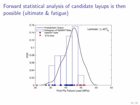
Table of Contents
Why Probabilistic Models
Composite Structures
Turbulent Aero(structural) dynamics
(Smart) Grid Integration
11 26
To explore new (multi-MW scale floating) concepts need to get beyond BEM
Physics not captured by BEM
Non-linear motion amp deflections Sweptwinglet blades
Unsteady aerodynamics
CFD still to costly for unsteady design
Vortex-based methods appropriate
But costly for unsteady design
Also want gradients for unsteady performance
12 26
stochastic input process solve system
equations
several realizations(only if needed)
analyze results
Γξ i(t)=f (uξ i(t))
Γ(t ξ)=f (u(t ξ))
several realizations
one stochastic solution
several deterministic solutions
Fundamentally we want to replace many time-domain simulations with a single solution in the stochastic space
13 26
We have adopted intrusive chaos (polynomial) methods to analyze in the stochastic domain
Expand wind inflow model with random phase angles ξ isin [minusπ π] as
Rminus1R uinfin(tn ξ) = ur (tn)Ψr (ξ)
r=0
Lots of groundwork on describing correlated wind fields with minimum number of ξ phase angles Expand circulate strength Γ (lift) as
Rminus1R Γ(tn ξ) = gr (tn)Ψr (ξ)
r =0
Functionals Ψr (ξ) define polynomials (exponentials) of random variable ξ
Choose form based on PDF of ξ Legendre polynomials for uniform distributions
14 26
Solution procedure is equivalent to one time-domain solve but obtain results for all possible ξ values
Use inner product (D Ψr (ξ)) lsquostochastic Galerkinrsquo projection
Orthogonality property of Ψr (ξ) when chosen correctly Equations for coefficients in time fall out
ur (tn) gr (tn)
Note that these solutions are functions of time
Not a Fourier transform Can handle non-linear time dependent effects
Output quantity calculations
Time-domain for specific ξ realization
Validation with time dependent code
Directly compute statistical moments from gr (tn) PDF reconstruction methods
All possible wind input fields evaluated simultaneously
15 26
Wersquove applied the stochastic Galerkin method to stationary bladeswings (lifting line)
tra
iling
fila
men
ts
Γ j(k
+1
)
k =
1
k =
M
i = N
+1
j= N
j= 1
i = 1
c)
xx
xx
x
r ijk
Γikshed
elements
x
x xxx
xxx x x x
x
xx
xx
xx
xxx
xxx
xX
ik
X(i+
1)k
x
x xxx
x
y
γ20
γ10
γ50 γN b N t
γ12Γ1(t n)
Γ2(t n)
Γ3(tn)
Γ4(tn)
Γ5(tn)
Γs 11
Γs 21
Γs 42H 3(s 51)
G3(s 23)
Γt 13
Γt 51
Nt elements
Nb e
lem
ents
γ31
16 26
Wersquove applied the stochastic Galerkin method to stationary bladeswings (lifting line)
span position [m]-25 -15 -5 5 15 25
circula
tion [m
2s
]
5
10
15
steady state stochastic at t=[68101214] s
wind speed [ms]8 10 12 8 10 12 8 10 12 8 10 12 8 10 12 8 10 12
tim
e [s]
0
5
10
15
wind bound circulation (deterministic) bound circulation (stochstic)
circulation [m2s]
9 11 13 9 11 13 9 11 13 9 11 13 9 11 13 9 11 13
17 26
and simplified BEM compared to 100 deterministic sample wind inputs
3 6 9 12 15 18
time [s]
0
10
20
30
element at rR=014
element at rR=086
18 26
Table of Contents
Why Probabilistic Models
Composite Structures
Turbulent Aero(structural) dynamics
(Smart) Grid Integration
19 26
Wind energyrsquos value depends on the grid-delivered product hopefully greater than the costs to provide it
Various components in levelized cost of energy Base materials ndash capital costs Aerostructural performance ndash power captureloads Variability in system costs captured with previous approaches
But value is different than costs Levelized avoided cost of energy (LACE)
LCOE estimates revenue requirements LACE estimates revenues available
Firming services costs
How to model variable grid system performance
20 26
The interconnected grid is large and complicated requiring efficient solutions methods
BPAT
BCHAAESO
WAUWNWMT
IPCO
AVA
PGE
PACW
PACE
WACM
PSCO
PNM
EPE
WALC
SRP
AZPS
IID
PSEISCL
TPWR
DOPDCHPD
DEAAGRMA
HGMATEPC
LDWP
BANC
TIDC
CFE
CISO
GCPDWWA
GRIF
GWA
NEVP
GRID
Boundaries are approximate and for illustrative purposes only
Western InterconnectionBalancing Authorities (38)
AESO - Alberta Electric System OperatorAZPS - Arizona Public Service CompanyAVA - Avista CorporationBANC - Balancing Authority of Northern CaliforniaBPAT - Bonneville Power Administration - TransmissionBCHA - British Columbia Hydro AuthorityCISO - California Independent System OperatorCFE - Comision Federal de ElectricidadDEAA - Arlington Valley LLCEPE - El Paso Electric CompanyGRMA - Gila River Power LPGRID - GridforceGRIF - Grith Energy LLCIPCO - Idaho Power Company
IID - Imperial Irrigation DistrictLDWP - Los Angeles Department of Water and PowerGWA - NaturEner Power Watch LLCNEVP - Nevada Power CompanyHGMA - New Harquahala Generating Company LLCNWMT - NorthWestern EnergyPACE - PaciCorp EastPACW - PaciCorp WestPGE - Portland General Electric CompanyPSCO - Public Service Company of ColoradoPNM - Public Service Company of New MexicoCHPD - PUD No 1 of Chelan CountyDOPD - PUD No 1 of Douglas CountyGCPD - PUD No 2 of Grant County
PSEI - Puget Sound EnergySRP - Salt River ProjectSCL - Seattle City LightTPWR - City of Tacoma Department of Public Utilities TEPC - Tucson Electric Power CompanyTIDC - Turlock Irrigation DistrictWACM - Western Area Power Administration Colorado-Missouri RegionWALC - Western Area Power Administration Lower Colorado RegionWAUW - Western Area Power Administration Upper Great Plains WestWWA - NaturEner Wind Watch LLC
011915hr
21 26
The power grid is modeled by a set of (non-)linear power flow equations
Distribution and transmission grid governing equations
[Pi Qi ] = f (Vi δi ) [Pik Qik ] = f (Vi Vk δik )
22 26
Cumulant-based analysis methods to handle stochastic generation and loads on each bus
Input definition Real Pi and imaginary Qi power injections represent generation and loads on each bus
Compute moments microv of the distributions Convert moments to cumulants κv of those distributions
Analysis method
Basic cumulant arithmetic for Y = AX κY v = Av κX v
We extended to cumulant tensors for correlated variables and polynomial functionals
Linearize polar form of equations amp truncate Rectangular form of power flow equation expansion rArr exact quadratic equation
Post-process results
[Vi δi Pik Qik ] outputs impacting costs etc Maximum-entropy PDF reconstruction from κv
23 26
IEEE 14 bus example with wind power generation and plug-in vehicle loads
24 26
Thanks for listening
Dr Curran Crawford
E-mail currancuvicca
Website wwwssdluvicca
Twitter SSDLab
Students
Composites Ghulam Mustafa
Aero Manuel Fluck Rad Haghi
Grid Trevor Williams Pouya Amid
25 26
- Why Probabilistic Models
- Composite Structures
- Turbulent Aero(structural) dynamics
- (Smart) Grid Integration
-
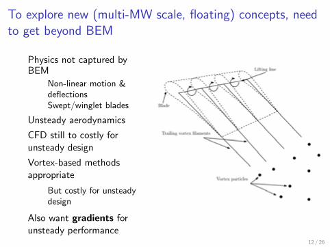
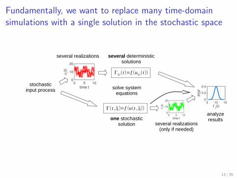
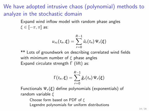
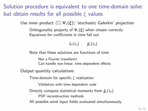
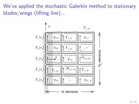
Wersquove applied the stochastic Galerkin method to stationary bladeswings (lifting line)
tra
iling
fila
men
ts
Γ j(k
+1
)
k =
1
k =
M
i = N
+1
j= N
j= 1
i = 1
c)
xx
xx
x
r ijk
Γikshed
elements
x
x xxx
xxx x x x
x
xx
xx
xx
xxx
xxx
xX
ik
X(i+
1)k
x
x xxx
x
y
γ20
γ10
γ50 γN b N t
γ12Γ1(t n)
Γ2(t n)
Γ3(tn)
Γ4(tn)
Γ5(tn)
Γs 11
Γs 21
Γs 42H 3(s 51)
G3(s 23)
Γt 13
Γt 51
Nt elements
Nb e
lem
ents
γ31
16 26
Wersquove applied the stochastic Galerkin method to stationary bladeswings (lifting line)
span position [m]-25 -15 -5 5 15 25
circula
tion [m
2s
]
5
10
15
steady state stochastic at t=[68101214] s
wind speed [ms]8 10 12 8 10 12 8 10 12 8 10 12 8 10 12 8 10 12
tim
e [s]
0
5
10
15
wind bound circulation (deterministic) bound circulation (stochstic)
circulation [m2s]
9 11 13 9 11 13 9 11 13 9 11 13 9 11 13 9 11 13
17 26
and simplified BEM compared to 100 deterministic sample wind inputs
3 6 9 12 15 18
time [s]
0
10
20
30
element at rR=014
element at rR=086
18 26
Table of Contents
Why Probabilistic Models
Composite Structures
Turbulent Aero(structural) dynamics
(Smart) Grid Integration
19 26
Wind energyrsquos value depends on the grid-delivered product hopefully greater than the costs to provide it
Various components in levelized cost of energy Base materials ndash capital costs Aerostructural performance ndash power captureloads Variability in system costs captured with previous approaches
But value is different than costs Levelized avoided cost of energy (LACE)
LCOE estimates revenue requirements LACE estimates revenues available
Firming services costs
How to model variable grid system performance
20 26
The interconnected grid is large and complicated requiring efficient solutions methods
BPAT
BCHAAESO
WAUWNWMT
IPCO
AVA
PGE
PACW
PACE
WACM
PSCO
PNM
EPE
WALC
SRP
AZPS
IID
PSEISCL
TPWR
DOPDCHPD
DEAAGRMA
HGMATEPC
LDWP
BANC
TIDC
CFE
CISO
GCPDWWA
GRIF
GWA
NEVP
GRID
Boundaries are approximate and for illustrative purposes only
Western InterconnectionBalancing Authorities (38)
AESO - Alberta Electric System OperatorAZPS - Arizona Public Service CompanyAVA - Avista CorporationBANC - Balancing Authority of Northern CaliforniaBPAT - Bonneville Power Administration - TransmissionBCHA - British Columbia Hydro AuthorityCISO - California Independent System OperatorCFE - Comision Federal de ElectricidadDEAA - Arlington Valley LLCEPE - El Paso Electric CompanyGRMA - Gila River Power LPGRID - GridforceGRIF - Grith Energy LLCIPCO - Idaho Power Company
IID - Imperial Irrigation DistrictLDWP - Los Angeles Department of Water and PowerGWA - NaturEner Power Watch LLCNEVP - Nevada Power CompanyHGMA - New Harquahala Generating Company LLCNWMT - NorthWestern EnergyPACE - PaciCorp EastPACW - PaciCorp WestPGE - Portland General Electric CompanyPSCO - Public Service Company of ColoradoPNM - Public Service Company of New MexicoCHPD - PUD No 1 of Chelan CountyDOPD - PUD No 1 of Douglas CountyGCPD - PUD No 2 of Grant County
PSEI - Puget Sound EnergySRP - Salt River ProjectSCL - Seattle City LightTPWR - City of Tacoma Department of Public Utilities TEPC - Tucson Electric Power CompanyTIDC - Turlock Irrigation DistrictWACM - Western Area Power Administration Colorado-Missouri RegionWALC - Western Area Power Administration Lower Colorado RegionWAUW - Western Area Power Administration Upper Great Plains WestWWA - NaturEner Wind Watch LLC
011915hr
21 26
The power grid is modeled by a set of (non-)linear power flow equations
Distribution and transmission grid governing equations
[Pi Qi ] = f (Vi δi ) [Pik Qik ] = f (Vi Vk δik )
22 26
Cumulant-based analysis methods to handle stochastic generation and loads on each bus
Input definition Real Pi and imaginary Qi power injections represent generation and loads on each bus
Compute moments microv of the distributions Convert moments to cumulants κv of those distributions
Analysis method
Basic cumulant arithmetic for Y = AX κY v = Av κX v
We extended to cumulant tensors for correlated variables and polynomial functionals
Linearize polar form of equations amp truncate Rectangular form of power flow equation expansion rArr exact quadratic equation
Post-process results
[Vi δi Pik Qik ] outputs impacting costs etc Maximum-entropy PDF reconstruction from κv
23 26
IEEE 14 bus example with wind power generation and plug-in vehicle loads
24 26
Thanks for listening
Dr Curran Crawford
E-mail currancuvicca
Website wwwssdluvicca
Twitter SSDLab
Students
Composites Ghulam Mustafa
Aero Manuel Fluck Rad Haghi
Grid Trevor Williams Pouya Amid
25 26
- Why Probabilistic Models
- Composite Structures
- Turbulent Aero(structural) dynamics
- (Smart) Grid Integration
-
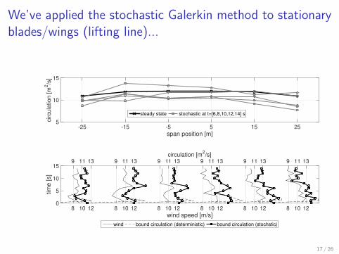
Wersquove applied the stochastic Galerkin method to stationary bladeswings (lifting line)
span position [m]-25 -15 -5 5 15 25
circula
tion [m
2s
]
5
10
15
steady state stochastic at t=[68101214] s
wind speed [ms]8 10 12 8 10 12 8 10 12 8 10 12 8 10 12 8 10 12
tim
e [s]
0
5
10
15
wind bound circulation (deterministic) bound circulation (stochstic)
circulation [m2s]
9 11 13 9 11 13 9 11 13 9 11 13 9 11 13 9 11 13
17 26
and simplified BEM compared to 100 deterministic sample wind inputs
3 6 9 12 15 18
time [s]
0
10
20
30
element at rR=014
element at rR=086
18 26
Table of Contents
Why Probabilistic Models
Composite Structures
Turbulent Aero(structural) dynamics
(Smart) Grid Integration
19 26
Wind energyrsquos value depends on the grid-delivered product hopefully greater than the costs to provide it
Various components in levelized cost of energy Base materials ndash capital costs Aerostructural performance ndash power captureloads Variability in system costs captured with previous approaches
But value is different than costs Levelized avoided cost of energy (LACE)
LCOE estimates revenue requirements LACE estimates revenues available
Firming services costs
How to model variable grid system performance
20 26
The interconnected grid is large and complicated requiring efficient solutions methods
BPAT
BCHAAESO
WAUWNWMT
IPCO
AVA
PGE
PACW
PACE
WACM
PSCO
PNM
EPE
WALC
SRP
AZPS
IID
PSEISCL
TPWR
DOPDCHPD
DEAAGRMA
HGMATEPC
LDWP
BANC
TIDC
CFE
CISO
GCPDWWA
GRIF
GWA
NEVP
GRID
Boundaries are approximate and for illustrative purposes only
Western InterconnectionBalancing Authorities (38)
AESO - Alberta Electric System OperatorAZPS - Arizona Public Service CompanyAVA - Avista CorporationBANC - Balancing Authority of Northern CaliforniaBPAT - Bonneville Power Administration - TransmissionBCHA - British Columbia Hydro AuthorityCISO - California Independent System OperatorCFE - Comision Federal de ElectricidadDEAA - Arlington Valley LLCEPE - El Paso Electric CompanyGRMA - Gila River Power LPGRID - GridforceGRIF - Grith Energy LLCIPCO - Idaho Power Company
IID - Imperial Irrigation DistrictLDWP - Los Angeles Department of Water and PowerGWA - NaturEner Power Watch LLCNEVP - Nevada Power CompanyHGMA - New Harquahala Generating Company LLCNWMT - NorthWestern EnergyPACE - PaciCorp EastPACW - PaciCorp WestPGE - Portland General Electric CompanyPSCO - Public Service Company of ColoradoPNM - Public Service Company of New MexicoCHPD - PUD No 1 of Chelan CountyDOPD - PUD No 1 of Douglas CountyGCPD - PUD No 2 of Grant County
PSEI - Puget Sound EnergySRP - Salt River ProjectSCL - Seattle City LightTPWR - City of Tacoma Department of Public Utilities TEPC - Tucson Electric Power CompanyTIDC - Turlock Irrigation DistrictWACM - Western Area Power Administration Colorado-Missouri RegionWALC - Western Area Power Administration Lower Colorado RegionWAUW - Western Area Power Administration Upper Great Plains WestWWA - NaturEner Wind Watch LLC
011915hr
21 26
The power grid is modeled by a set of (non-)linear power flow equations
Distribution and transmission grid governing equations
[Pi Qi ] = f (Vi δi ) [Pik Qik ] = f (Vi Vk δik )
22 26
Cumulant-based analysis methods to handle stochastic generation and loads on each bus
Input definition Real Pi and imaginary Qi power injections represent generation and loads on each bus
Compute moments microv of the distributions Convert moments to cumulants κv of those distributions
Analysis method
Basic cumulant arithmetic for Y = AX κY v = Av κX v
We extended to cumulant tensors for correlated variables and polynomial functionals
Linearize polar form of equations amp truncate Rectangular form of power flow equation expansion rArr exact quadratic equation
Post-process results
[Vi δi Pik Qik ] outputs impacting costs etc Maximum-entropy PDF reconstruction from κv
23 26
IEEE 14 bus example with wind power generation and plug-in vehicle loads
24 26
Thanks for listening
Dr Curran Crawford
E-mail currancuvicca
Website wwwssdluvicca
Twitter SSDLab
Students
Composites Ghulam Mustafa
Aero Manuel Fluck Rad Haghi
Grid Trevor Williams Pouya Amid
25 26
- Why Probabilistic Models
- Composite Structures
- Turbulent Aero(structural) dynamics
- (Smart) Grid Integration
-
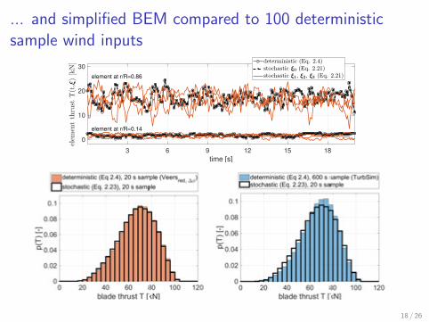
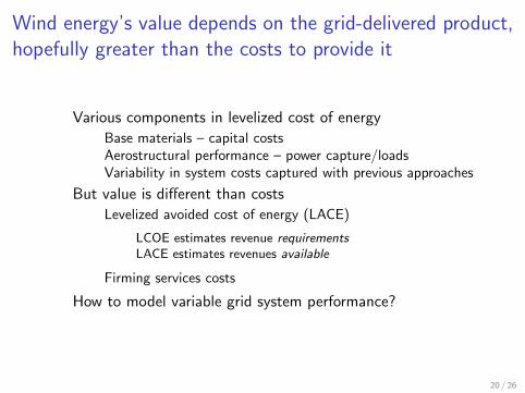
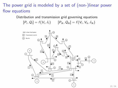
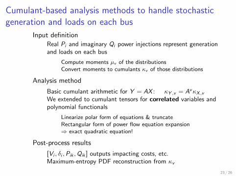
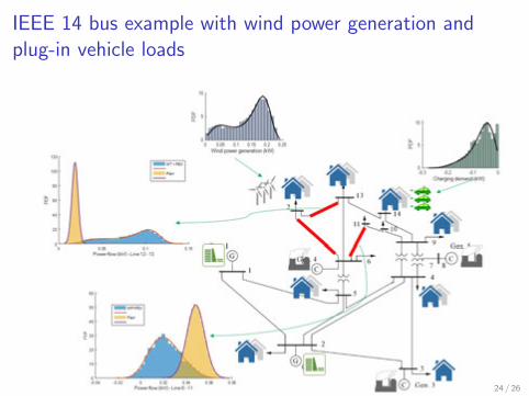