Probabilistic wind contouring and hazard mapping of ...philsciletters.org/2014/PSL...

ARTICLE

Probabilistic wind contouring

and hazard mapping of

barangay San Juan, Surigao City,

Surigao del Norte, Philippines

Marvin Aldrich R. Salazar1 and Lessandro Estelito O. Garciano2,* 1Undergraduate Student, Department of Civil Engineering, De La Salle University, Manila, Philippines

2Associate Professor, Department of Civil Engineering, De La Salle University, Manila, Philippines

E ach year the resilience of the Filipino people is

challenged by several natural disasters such as ty-

phoons, floods and storm surges. Typhoons, which

have the highest frequency and which cost the most

damage continue to take their toll on lives, prop-

erty, livelihood and, worse, inflict untold trauma on affected

families. In view of the risks posed by extreme wind speeds

(during typhoons), the authors take a step to address this problem

by developing a probabilistic wind contour map and wind hazard

map of a specific barangay. The maps developed for barangay

San Juan, Surigao City, Surigao del Norte, can be used by the

local government unit and residents to evaluate and possibly

reduce the risks in this area during strong typhoons. The high-

lights in the development of the maps are the following: (a) the

generalized extreme value distribution was used to model the

annual extreme wind speeds and the extrapolation of 50, 100 and

150 year return wind speeds, (b) application of correction factors

to account for shielding effects of houses, and (c) the use of geo-

graphic information technology to create contour and hazard

maps. Hopefully, the results can be replicated for other areas in

the country as a step towards “climate-proofing” our communi-

ties.

275 Vol. 7 | No. 2 | 2014 Philippine Science Letters

*Corresponding author

Email Address: [email protected]

Submitted: June 11, 2014

Revised: July 23, 2014

Accepted: June 13, 2014

Published: July 30, 2014

Editor-in-charge: Amador C. Muriel

Reviewer: Amador C. Muriel

INTRODUCTION

Recent typhoons such as Pablo and super typhoon Yolanda

have exceeded the basic wind speeds of the three wind zones of

the current National Structural Code of the Philippines (NSCP).

These extreme events left everybody pondering how we can

adapt to the changing weather patterns that have caused a lot of

damage to life, livelihood and infrastructure. It can be seen from

Table 1 that the total cost of damage for selected natural disas-

ters in the country from 2000 to 2012 was around US$ 3 billion

(CRED 2013). In Table 2 we can see that storm had the highest

occurrence of seven in 2012 (CRED 2013). During this year, the

most significant natural disaster was due to typhoon Pablo

(international code name: Bopha). This typhoon was considered

to be the strongest to hit Mindanao in decades (Legaspi 2012)

that left more than 9700 families homeless (ANC 2012). The

National Disaster Risk Reduction and Management Council

(NDRRMC 2012) estimated 1067 deaths and about US$ 86 mil-

lion worth of damage caused by typhoon Pablo. This total dam-

age is about 91% of the total damage from significant natural

disasters in the country as shown in Table 2.

It is even alarming that stronger-than-before typhoons are

increasingly making landfall in Southern Philippines (Alonzo

2011, BBC News Asia 2009). Figure 1 shows Typhoon Pablo

making landfall near Baganga, Davao Oriental with maximum

sustained winds of 185 kph and a maximum wind speed of 280

kph. In 2013, super typhoon Yolanda made landfall in Guian,

KEYWORDS

extreme wind speeds, generalized extreme value distribution,

resilience, typhoons, wind hazard map

Samar with a reported speed of 300 kph, considered the strongest

in the world to make landfall. This typhoon left 6,200 deaths,

30,000 injured, and 1,140,332 damaged houses with a total dam-

age of 40 billion pesos (NDRRMC 2013). Figure 2 shows a part

of the roof attached to a steel truss that was blown away in

Northern Cebu during typhoon Yolanda. The current NSCP

(ASEP 2010) divides the country into three wind zones with 125,

200 and 250 kph as the basic wind speeds. Using new methods

in extreme value theory, there have been several proposals to

update this map. Garciano et al. (2005) proposed a six-zone map


with 10 m/s interval per zone, while Pacheco et al. (2007) pro-

posed a 5-zone map with intervals of 125, 150, 200, 250 and

300. Recently De Leoz et al. (2014) prepared a four-zone wind

map and contour maps using the generalized extreme value

(GEV) distribution and recent extreme wind speed data from the

Philippine Atmospheric, Geophysical and Astronomical Services

(PAGASA). Unfortunately, damage to roofs and cladding still

Year Death

Toll Homeless Injured Affected

Cost of Damage Million

(USD)

2000 748 125,250 393 6,425,002 89.76

2001 630 100,000 480 3,624,958 109.64

2002 320 3,000 233 1,211,212 17.54

2003 352 83,203 75 678,761 42.30

2004 1,950 8,700 1,321 3,263,076 138.87

2005 39 - - 213,057 2.52

2006 2,984 - 2,703 8,612,817 347.28

2007 129 - 24 2,023,092 16.82

2008 959 54,645 1,015 8,459,896 481.20

2009 1,307 110 900 13,352,484 962.11

2010 1,113 - 124,096 5,581,507 335.09

2011 1,989 - 6,703 11,729,947 730.03

2012 379 - 173 5,889,176 94.39

Total 12,899 374,908 138,116 71,073,985 3,367.53

Table 1. Cost of damage due to selected natural disasters in the

Philippines (CRED 2013).

Year Drought Earthquake Epidemic Flood

Mass

movement

dry

Mass

movement

wet

Storm Volcano Total

2000 0 0 1 3 1 1 6 1 13

2001 0 0 0 3 0 0 6 2 11

2002 1 1 0 4 0 0 6 0 12

2003 0 0 1 1 0 1 8 0 11

2004 0 0 1 3 0 1 8 0 13

2005 0 0 0 2 0 0 2 0 4

2006 0 0 0 6 0 3 10 1 20

2007 1 0 0 5 0 0 9 1 16

2008 0 0 0 8 0 0 11 0 19

2009 0 1 0 8 0 0 14 1 24

2010 0 0 1 9 0 0 3 1 14

2011 0 1 3 15 0 0 12 2 33

2012 0 3 1 5 0 0 7 0 18

Total 2 6 8 72 1 7 102 9 207

Table 2. Natural Disasters in the Philippines (CRED 2013).

Figure 1. Track of the typhoon Pablo (source: PAGASA).

Figure 2. Damage due to Supertyphoon Yolanda (source R.

Harmer).

Vol. 7 | No. 2 | 2014 277 Philippine Science Letters

In this paper, the authors take into account gusts of different

return periods and apply a correction factor for the shielding

effect that was developed through a study using wind tunnel test-

ing. The application of the model to the wind speed maxima

gives the scenario for the extreme wind speeds that may be ex-

perienced by the point in the area considered. Each layer is then

classified through techniques of interpolation to arrive at a con-

toured map showing the different levels of wind that can be felt.

METHODOLOGY

Probabilistic Wind Hazard Analysis (PWHA)

Figure 4. Probabilistic Wind Hazard Analysis (PWHA).

The key steps in developing the PWHA are shown in Figure

4 (Salazar 2014). The details of each task are discussed below.

A. Data collection and assimilation

In this stage, the site and its demarcation are identi-

fied. A desk study is then conducted to determine the

following: the plan dimensions of the structures and the eleva-

tion

the grouping and aggregating of the structures, if

possible (grid spacing is also established)

the horizontal and displacement angles for the cor-

rection factor model of each grouping

the longitude and latitude of the structures

a digital elevation map of the site

Handheld Global Positioning System (GPS) devices are

occurs for low-rise and low-cost residential structures and, espe-

cially, for informal settlements during extreme wind events. In

the authors opinion, these roof and cladding failures continue to

occur due to the following: (a) the structural components were

not “engineered”, but were based on design prescription or con-

struction experience, rather than by calculating demand, e.g., live

load, dead load, earthquake, wind, etc., and comparing it with

the capacity of the structural component, (b) the critical struc-

tural component may have deteriorated over time increasing the

probability of failure, (c) extreme wind speeds may have signifi-

cantly increased in strength due to climate change patterns, and

(d) areas rarely hit by strong typhoons are experiencing these

phenomena. Figure 3 is a graphical representation of the reasons

that contribute to the increase in the probability of failure of

roofs and cladding during extreme wind speed events.

Figure 3. Increase in the probability of failure due to an increas-ing load (S) and a deteriorating resistance (R).

In this regard, the authors see a need to develop a method for

a site-specific wind hazard mapping of a particular area. There

are several ways to create a wind hazard map. One of the com-

mon methods used is through zoning the entire country. The

current NSCP used zoning by gathering the annual wind speed

for each PAGASA station and dividing the country into three

major zones. This however does not take into account specific

areas with high wind speeds that are included inside a zone with

a weaker wind provision such as in zone 3. A study in the United

States proposes that a single wind zone map of the United States

should be changed into three regions (Vickery et al. 2010). This

divides a country into three separate entities and, in each region,

zoning is done per group of wind stations. Another approach to

hazard mapping is through region scaling and testing using a

wind tunnel. This takes into account the topography of the struc-

tures, as well as shielding effects. The sensors in the model pro-

duces different wind speeds that are then contoured resulting in a

hazard map.

structural dimen-

sions

Data Collection

and

assimilation grid spacing

annual extreme

wind speeds

angular dimen-

sions

effective wind

area

MLE of GEV

parameters

correction factor

for shielding

effects

GEV modeling of

extreme wind

speeds

Wind speed

modeling

and simulation

group structure

wind speed

Wind Contour

Map

and Hazard Map

Validation of results through site measure-

ments

kriging interpolation

method Geostatistical analysis

Geographic Information Technology


(3)

where αh and αv are the horizontal and vertical angles in degrees,

respectively, and Co = 0.8548, C1 = 0.7677, C2 = 0.6261. Note

that any value of αh above 140° does not significantly change the

value of the correction factor.

Figure 5. Orthogonal set-up for correction factor.

In the house groups, there were displacements that had oc-

curred when measuring the structural dimensions. These dis-

placements are the description of the horizontal shift that occurs

when the line bisecting the horizontal angle does not coincide

with the line that connects the centers of the shielding and

shielded structures (see Figure 6). A new angle (αd) is introduced

to describe this relationship.

Figure 6. Correction of Orthogonal Model.

The orthogonal pressure coefficient is now denoted by:

where αd is the displacement angle, e is the Euler’s number, C0 =

0.5046, C1= 0.2216 and C2 = -0.4718. The displacement angle

was limited to be in the range of 0 – 90o as observed in the study.

used to verify the longitude and latitude of the struc-

tures.

data gathering of available yearly extreme wind

speeds from PAGASA

B. Wind speed modeling and simulation

The obtained extreme wind speeds are fitted to a

GEV distribution using a maximum likelihood estimate

(MLE). The parameters of the GEV are used to extrapo-

late 50, 100 and 150-year return wind speeds. Estimat-

ing shielding factors that determine the orthogonal cor-

rection factor due to shielding effects and correction

due to displacement.

C. GIT (geographic information technology)

Data obtained during the above stages are con-

verted into shape files and encoded into a GIT software

such as ArcGIS (Kennedy 2009). Contour and hazard

mapping are developed using geostatistical analysis and

the Kriging interpolation method.

D. Validation of results through site measurements

Generalized extreme value (GEV) model

The GEV model encompasses the three distributions, e.g.,

Gumbel, Frechet and Weibull, and is defined by the following

equation (Coles 2001):

(1)

where μ is the location parameter, ξ is the shape parameter and σ

(>0) is the scale parameter.

The parameters of this distribution are estimated using MLE.

Extrapolation of return level wind speeds is determined using the

following equation:

(2)

where xp is the return level.

Orthogonal Correction factor

When multiple structures stand in the area where wind will

flow, shielding effects occur between these structures. The appli-

cation of a correction factor is based on the orthogonal model

where two buildings are parallel aligned for a wind tunnel ex-

periment (Sharag-Eldin 2007). The test was done considering

two structures that are parallel to each other, one shielding an-

other. The line connecting the center of both buildings is perpen-

dicular to the face of each one and parallel to the wind direction

(see Figure 5).

The correction factor considering the orthogonal model is

shown below.

αh

Shielding Structure Shielded Structure Wind

αh / 2

αd

Win

d D

irec

tio

n

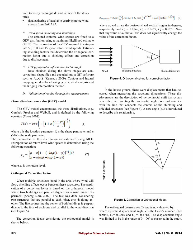
RESULTS AND ANALYSIS

Study Area

Surigao City is the capital city of Surigao del Norte (Figure 7a)

located in the southeastern part of the Philippines. The city falls

under Type II climate in a country with four main climate re-

gimes. This means there is no definite dry season, but with a

very pronounced maximum rainfall from November to January.

The monthly extreme precipitation recorded in Surigao City was

around 583 mm during the month of November 2008. The city

proper is composed of three barangays namely: Washington,

Taft and San Juan (which is the study area) as shown in Figure

7b. Barangay San Juan has a total land area of 0.45 sq. km. It is

bounded by the sea in the north and by barangays Rizal, Wash-

ington and Sabang in the south, east and west, respectively. In

2005, the number of households in barangay San Juan was 2,665

according to the minimum basic needs survey of the City Plan-

ning and Development Office of Surigao City. This number is

expected to increase to 3,413 by 2020.

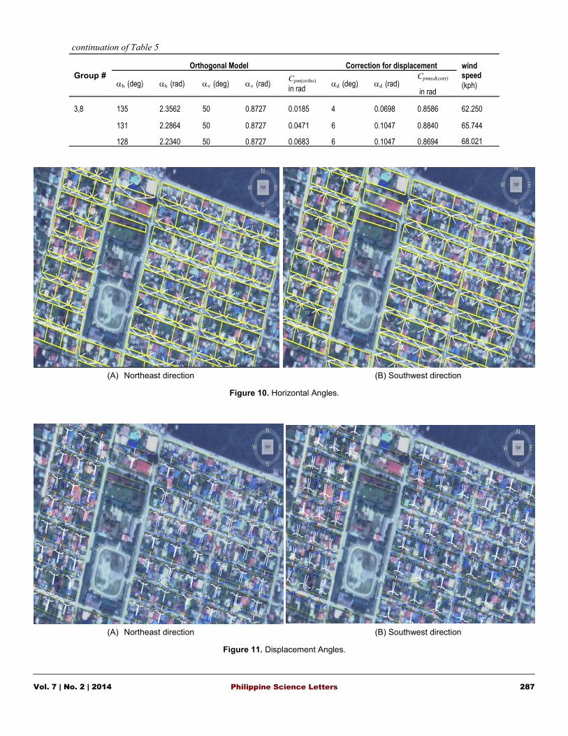
House grouping, angle determination and establishing coor-

dinates

Using the raster images of Surigao City, house groupings

were created using AutoCAD. The school (in the middle of Fig-

ure 8) was not included because it is considered an essential fa-

cility hence no wind reduction is applied. The determination of

angles was done for two directions: one when wind is expected

to come from the northeast (NE), the other when the wind is

expected from the southwest (SW). The angles were determined

using the dim-angular function of AutoCAD. The horizontal

angle (αh) defines the angle set by the shielding block, with the

reference point being the midpoint of the shielded structure.


Since two directions are considered, two sets of horizontal an-

gles are also considered as shown in Figure 8. The displacement

angle (αd) is a function of the horizontal angle. The projected

line from half of the horizontal angle (αh) would intersect the

shielding block. The angle formed by the perpendicular of the

projected line and the intersection between the projected line and

shielding block is defined as the displacement angle. Since the

houses are arranged in a grid manner, only a few changes in the

horizontal angles were noted. Since the displacement angle is a

function of the horizontal angle, only a small difference is ob-

servable.

Figure 8. Barangay San Juan house grouping.

The coordinates of each midpoint of the face of the shielded

group were determined because these are the points at which the

(A) Surigao del Norte (B) Barangay San Juan

Figure 7. Barangay San Juan, Surigao City, Surigao del Norte.

wind speed is tabulated. Table 3 is the complete list of the coor-

dinates of each house grouping.


Table 3. Coordinates of midpoints for NE and SW direction.

Group No.

Northeast Southwest

Longitude Latitude Longitude Latitude

1,1 125.487213° 9.788275° 125.487905° 9.790911°

125.486763° 9.788393° 125.487461° 9.791028°

125.486319° 9.788529° 125.486999° 9.791149°

1,2 125.487263° 9.788658° 125.487823° 9.790488°

125.486885° 9.788767° 125.487361° 9.790600°

125.486441° 9.788901° 125.486919° 9.790729°

1,3 125.487356° 9.789037° 125.487710° 9.790083°

125.486949° 9.789123° 125.487199° 9.790218°

125.486516° 9.789263° 125.486767° 9.790345°

1,4 125.487444° 9.789426° 125.487620° 9.789721°

125.487087° 9.789522° 125.487124° 9.789859°

125.486633° 9.789651° 125.486742° 9.789966° 1,5

125.487587° 9.789786° 125.487484° 9.789356°

125.487158° 9.789910° 125.487011° 9.789480°

125.486743° 9.790032° 125.486592° 9.789601° 1,6

125.487713° 9.790148° 125.487356° 9.788967°

125.487242° 9.790289° 125.486884° 9.789098°

125.486862° 9.790398° 125.486461° 9.789228° 1,7

125.487769° 9.790566° 125.487267° 9.788604°

125.487378° 9.790660° 125.486834° 9.788735°

125.486945° 9.790792° 125.486363° 9.788867° 1,8

125.487909° 9.790954° 125.487146° 9.788224°

125.487500° 9.791075° 125.486701° 9.788343°

125.487052° 9.791196° 125.486253° 9.788463° 2,1

125.485355° 9.787592° 125.486499° 9.791287°

125.484929° 9.787697° 125.486095° 9.791419°

125.484510° 9.787810° 125.485595° 9.791543° 2,2

125.485489° 9.787957° 125.486406° 9.790864°

125.485056° 9.788069° 125.485941° 9.791007°

125.484595° 9.788190° 125.485425° 9.791141° 2,3

125.485627° 9.788303° 125.486327° 9.790460°

125.485143° 9.788454° 125.485827° 9.790593°

125.484722° 9.788587° 125.485295° 9.790746°

Group No.

Northeast Southwest


2,4 125.485747° 9.788694° 125.486169° 9.790115°

125.485291° 9.788831° 125.485711° 9.790243°

125.484822° 9.788958° 125.485203° 9.790384° 2,5

125.485829° 9.789074° 125.486109° 9.789734°

125.485423° 9.789201° 125.485599° 9.789881°

125.484965° 9.789325° 125.485076° 9.790025° 2,6

125.485930° 9.789431° 125.485971° 9.789362°

125.485490° 9.789574° 125.485513° 9.789478°

125.485051° 9.789701° 125.484991° 9.789624° 2,7

125.486087° 9.789804° 125.485853° 9.788991°

125.485634° 9.789935° 125.485398° 9.789123°

125.485141° 9.790068° 125.484826° 9.789279° 2,8

125.486215° 9.790168° 125.485754° 9.788602°

125.485728° 9.790318° 125.485293° 9.788745°

125.485280° 9.790446° 125.484751° 9.788908° 2,9

125.486304° 9.790544° 125.485611° 9.788241°

125.485854° 9.790683° 125.485160° 9.788384°

125.485333° 9.790838° 125.484665° 9.788524° 2,10

125.486425° 9.790948° 125.485458° 9.787873°

125.485971° 9.791078° 125.485022° 9.787999°

125.485497° 9.791206° 125.484572° 9.788131° 2,11

125.486548° 9.791355° 125.485342° 9.787540°

125.486105° 9.791466° 125.484863° 9.787659°

125.485597° 9.791591° 125.484393° 9.787776° 3,1

125.483309° 9.789344° 125.484003° 9.792011°

125.482951° 9.789449° 125.483705° 9.792087°

125.482618° 9.789541° 125.483317° 9.792183° 3,2

125.483388° 9.789735° 125.483919° 9.791588°

125.483025° 9.789851° 125.483584° 9.791675°

125.482697° 9.789942° 125.483203° 9.791781° 3,3

125.483489° 9.790120° 125.483792° 9.791177°

125.483120° 9.790225° 125.483445° 9.791268°

125.482772° 9.790317° 125.483102° 9.791372°

Continuation of Table 3

Continued on

the next page

Shielding effect

With all the parameters determined, by the application of the

shielding effect equation given in Eq. 3, orthogonal effects were

obtained. Correction for the equation was then done to account

for the displacement angle. The output is the correction factor for

the shielding effect Cpmαd(corr). Two directions were considered as

shown in Tables 4 (NE) and 5 (SW).

Monthly extreme wind data from the Surigao, Surigao del

Norte station were obtained. The time frame was from 1961 to

2012. The data obtained were found to have two prevailing di-

rections: SW and NE as shown in Figures 10 and 11. The zero

values in these figures signify no data for that year.

Using R-software, the GEV parameters were obtained using

MLE. For NE extreme wind speeds, the following parameters

were obtained: μ = 13.68, σ = 3.36 and ξ = 0.17, and for SW

extreme wind speeds: μ = 16.70, σ = 5.62 and ξ = 0.11. From

these values, we can see that wind from the SW direction will be

greater compared to the NE despite having the highest recorded

wind speed of 56 m/s or 201 kph. Table 6 shows the extrapolated

50, 100 and 150-year return wind speeds obtained using Eq. 2.

Validating the results

The theoretical model in Eq. 4 was validated through man-

ual gathering of wind speeds for both shielding (Figure 12a) and


shielded (Figure 12b) blocks. Handheld anemometers were used

for this purpose. The correction factor is then applied to the wind

speed of the shielding structure and then compared with the ac-

tual wind speed observed from the shielded block.

Figure 13 shows the points (dots) where the actual wind

speeds were observed at the site. This represents the first row

shielding the second row and the second row shielding the third

row of the structure. The condition of “no obstruction” was also

tested by placing the instruments on the roadside (facing Surigao

sea) where there are no shielding structures to be considered.

Ten-minute average wind speeds were gathered as used by PA-

GASA.

Table 7 shows the 10-minute average wind speed gathered

at the locations indicated above. A comparison of the actual

gathered data of the shielded block and the theoretical applica-

tion of the correction factor to the shielding block was done

through an Analysis of Variance (ANOVA, Zar 1984). The re-

sults show that the F-values are less than the F-critical values.

This means that there are no significant differences between the

theoretical values and the actual values. The variance is accept-

able and thus supports the model given in Eq. 4. However, group

1,1,3 did not exhibit this support. The plausible cause of this is

the sudden change in wind direction, which invalidates Eq. 4

since the theory assumes that the wind is perpendicular to the

structure. The maximum three-second gusts every 10 minutes

were also gathered at the same points. The results show an ac-

ceptable support for the theoretical model. This means that on

most test points the F-value is less than the F-critical value.

The data confirm that there is, in fact, a decrease in wind

speed due to shielding effects of an obstructing structure.

Contour maps

With the correction factor obtained, based on per row of

houses, applied on the gust per return period, and determination

of the coordinates through GPS, contouring and spatial analysis

were done. The basis for the contour maps is the wind speed per

structure at elevation Z and an equal method of contouring. The

results are six maps that consider NE (Figure 14) and SW

(Figure 15) directions, and the 50, 100 and 150-year return lev-

els.

The contour maps are divided into 10 kph intervals of wind

speeds. This shows how the shielding blocks affect wind. It is

notable that at the beginning and at the end, the contour may be a

little distorted. The plausible cause for this is the data points at

which the contour is done. The end points for the map may not

be well defined in the contour, causing some errors in the lines.

This, however, does not affect the results because it can still be

interpreted that the wind speed at the nearby contour lines is of

the value it is denoted by. The contour lines therefore show how

the wind is reduced per house group due to the shielding effect.

Group No.

Northeast Southwest


3,4 125.483609° 9.790509° 125.483681° 9.790823°

125.483275° 9.790616° 125.483357° 9.790897°

125.482937° 9.790710° 125.482968° 9.791016°

3,5 125.483737° 9.790889° 125.483584° 9.790451°

125.483378° 9.790989° 125.483221° 9.790557°

125.483004° 9.791074° 125.482854° 9.790648°

3,6 125.483802° 9.791255° 125.483492° 9.790065°

125.483475° 9.791341° 125.483108° 9.790161°

125.483095° 9.791437° 125.482748° 9.790250°

3,7 125.483929° 9.791650° 125.483348° 9.789721°

125.483609° 9.791758° 125.483018° 9.789795°

125.483244° 9.791859° 125.482654° 9.789896°

3,8 125.484005° 9.792052° 125.483264° 9.789264°

125.483711° 9.792148° 125.482914° 9.789367°

125.483374° 9.792246° 125.482520° 9.789482°

Continuation of Table 3

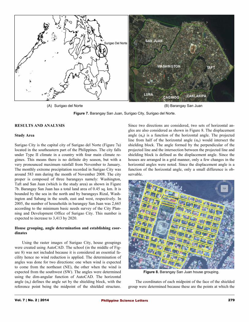
Table 4. Shielding correction factors for NE direction and corresponding wind speed.


Group

No.

Orthogonal Model Correction for displacement wind speed

(kph) h (deg) h (rad) v (deg) v (rad) Cpm(ortho) in rad

d (deg) d (rad) Cpmd(corr)

in rad

1,1 137 2.3911 50 0.8727 0.0040 6 0.1047 0.9211 106.789

137 2.3911 50 0.8727 0.0040 7 0.1222 0.9425 109.262

137 2.3911 50 0.8727 0.0040 6 0.1047 0.9211 106.789

1,2 133 2.3213 50 0.8727 0.0328 8 0.1396 0.9474 101.172

133 2.3213 50 0.8727 0.0328 8 0.1396 0.9474 103.514

133 2.3213 50 0.8727 0.0328 8 0.1396 0.9474 101.172

1,3 129 2.2515 50 0.8727 0.0613 10 0.1745 0.9914 100.303

129 2.2515 50 0.8727 0.0613 10 0.1745 0.9914 102.625

129 2.2515 50 0.8727 0.0613 6 0.1047 0.8740 88.427

1,4 133 2.3213 50 0.8727 0.0328 8 0.1396 0.9474 95.027

133 2.3213 50 0.8727 0.0328 8 0.1396 0.9474 97.227

133 2.3213 50 0.8727 0.0328 8 0.1396 0.9474 83.775

1,5 131 2.2864 50 0.8727 0.0471 5 0.0873 0.8545 81.201

131 2.2864 50 0.8727 0.0471 5 0.0873 0.8545 83.081

131 2.2864 50 0.8727 0.0471 5 0.0873 0.8545 71.586

1,6 128 2.2340 50 0.8727 0.0683 6 0.1047 0.8694 70.598

127 2.2166 50 0.8727 0.0753 6 0.1047 0.8651 71.872

127 2.2166 50 0.8727 0.0753 6 0.1047 0.8651 61.929

1,7 133 2.3213 50 0.8727 0.0328 4 0.0698 0.8401 59.310

132 2.3038 50 0.8727 0.0400 6 0.1047 0.8894 63.926

132 2.3038 50 0.8727 0.0400 5 0.0873 0.8611 53.330

1,8 131 2.2864 50 0.8727 0.0471 5 0.0873 0.8545 50.681

131 2.2864 50 0.8727 0.0471 5 0.0873 0.8545 54.625

131 2.2864 50 0.8727 0.0471 5 0.0873 0.8545 45.571

2,1 137 2.3911 50 0.8727 0.0040 5 0.0873 0.9000 104.343

137 2.3911 50 0.8727 0.0040 4 0.0698 0.8791 101.918

137 2.3911 50 0.8727 0.0040 5 0.0873 0.9000 104.343

2,2 129 2.2515 50 0.8727 0.0613 6 0.1047 0.8740 91.198

129 2.2515 50 0.8727 0.0613 10 0.1745 0.9914 101.043

129 2.2515 50 0.8727 0.0613 10 0.1745 0.9914 103.446

2,3 131 2.2864 50 0.8727 0.0471 8 0.1396 0.9404 85.760

131 2.2864 50 0.8727 0.0471 8 0.1396 0.9404 95.017

131 2.2864 50 0.8727 0.0471 8 0.1396 0.9404 97.278

continued on the next page

continuation of Table 4


Group

No.




in rad

2,4 140 2.4435 50 0.8727 -0.0178 4 0.0698 0.9141 78.393

140 2.4435 50 0.8727 -0.0178 4 0.0698 0.9141 86.855

140 2.4435 50 0.8727 -0.0178 4 0.0698 0.9141 88.921

2,5 133 2.3213 50 0.8727 0.0328 4 0.0698 0.8401 65.858

133 2.3213 50 0.8727 0.0328 6 0.1047 0.8951 77.748

133 2.3213 50 0.8727 0.0328 4 0.0698 0.8401 74.703

2,6 143 2.4958 50 0.8727 -0.0399 2 0.0349 0.9593 63.178

143 2.4958 50 0.8727 -0.0399 2 0.0349 0.9593 74.584

143 2.4958 50 0.8727 -0.0399 2 0.0349 0.9593 71.663

2,7 138 2.4086 50 0.8727 -0.0032 2 0.0349 0.8549 54.008

138 2.4086 50 0.8727 -0.0032 3 0.0524 0.8720 65.040

138 2.4086 50 0.8727 -0.0032 3 0.0524 0.8720 62.493

2,8 132 2.3038 50 0.8727 0.0400 4 0.0698 0.8316 44.910

132 2.3038 50 0.8727 0.0400 4 0.0698 0.8316 54.085

132 2.3038 50 0.8727 0.0400 4 0.0698 0.8316 51.966

2,9 141 2.4609 50 0.8727 -0.0252 1 0.0175 0.9215 41.386

141 2.4609 50 0.8727 -0.0252 1 0.0175 0.9215 49.841

141 2.4609 50 0.8727 -0.0252 1 0.0175 0.9215 47.889

2,10 137 2.3911 50 0.8727 0.0040 4 0.0698 0.8791 36.384

134 2.3387 50 0.8727 0.0257 4 0.0698 0.8491 42.320

130 2.2689 50 0.8727 0.0542 5 0.0873 0.8482 40.619

2,11 134 2.3387 50 0.8727 0.0257 7 0.1222 0.9263 33.703

137 2.3911 50 0.8727 0.0040 3 0.0524 0.8583 36.324

140 2.4435 50 0.8727 -0.0178 2 0.0349 0.8930 36.274

3,1 135 2.3562 50 0.8727 0.0185 6 0.1047 0.9075 105.207

131 2.2864 50 0.8727 0.0471 6 0.1047 0.8840 102.486

127 2.2166 50 0.8727 0.0753 5 0.0873 0.8313 96.369

3,2 129 2.2515 50 0.8727 0.0613 4 0.0698 0.8085 85.062

128 2.2340 50 0.8727 0.0683 4 0.0698 0.8017 82.159

126 2.1991 50 0.8727 0.0823 4 0.0698 0.7890 76.038

3,3 126 2.1991 50 0.8727 0.0823 4 0.0698 0.7890 67.117

123 2.1468 50 0.8727 0.1033 5 0.0873 0.8128 66.776

119 2.0769 50 0.8727 0.1308 6 0.1047 0.8386 63.766




Group

No.




in rad

3,4 128 2.2340 50 0.8727 0.0683 7 0.1222 0.9009 60.463

127 2.2166 50 0.8727 0.0753 7 0.1222 0.8974 59.925

126 2.1991 50 0.8727 0.0823 6 0.1047 0.8610 54.902

3,5 124 2.1642 50 0.8727 0.0963 5 0.0873 0.8170 49.397

127 2.2166 50 0.8727 0.0753 4 0.0698 0.7952 47.650

129 2.2515 50 0.8727 0.0613 4 0.0698 0.8085 44.390

3,6 130 2.2689 50 0.8727 0.0542 4 0.0698 0.8158 40.297

128 2.2340 50 0.8727 0.0683 4 0.0698 0.8017 38.199

126 2.1991 50 0.8727 0.0823 5 0.0873 0.8262 36.675

3,7 129 2.2515 50 0.8727 0.0613 4 0.0698 0.8085 32.581

127 2.2166 50 0.8727 0.0753 4 0.0698 0.7952 30.374

125 2.1817 50 0.8727 0.0893 3 0.0524 0.7410 27.178

3,8 125 2.1817 50 0.8727 0.0893 5 0.0873 0.8215 26.764

127 2.2166 50 0.8727 0.0753 5 0.0873 0.8313 25.249

129 2.2515 50 0.8727 0.0613 6 0.1047 0.8740 23.754

Table 5. Shielding correction factors for SW direction and corresponding wind speed.

Group # Orthogonal Model Correction for displacement wind

speed

(kph) h (deg) h (rad) v (deg) v (rad) Cpm(ortho)

in rad d (deg) d (rad)

Cpmd(corr)

in rad

1,1 131 2.2864 50 0.8727 0.0471 8 0.1396 0.9404 148.533

131 2.2864 50 0.8727 0.0471 8 0.1396 0.9404 148.533

131 2.2864 50 0.8727 0.0471 8 0.1396 0.9404 148.533

1,2 133 2.3213 50 0.8727 0.0328 8 0.1396 0.9474 140.720

132 2.3038 50 0.8727 0.0400 6 0.1047 0.8894 132.111

132 2.3038 50 0.8727 0.0400 6 0.1047 0.8894 132.111

1,3 129 2.2515 50 0.8727 0.0613 5 0.0873 0.8422 118.520

128 2.2340 50 0.8727 0.0683 6 0.1047 0.8694 114.861

128 2.2340 50 0.8727 0.0683 6 0.1047 0.8694 114.861

1,4 131 2.2864 50 0.8727 0.0471 6 0.1047 0.8840 104.774

131 2.2864 50 0.8727 0.0471 5 0.0873 0.8545 98.149

131 2.2864 50 0.8727 0.0471 7 0.1222 0.9125 104.815






speed



Cpmd(corr)

in rad

1,5 133 2.3213 50 0.8727 0.0328 4 0.0698 0.8401 88.021

133 2.3213 50 0.8727 0.0328 4 0.0698 0.8401 82.455

133 2.3213 50 0.8727 0.0328 5 0.0873 0.8681 90.995

1,6 129 2.2515 50 0.8727 0.0613 6 0.1047 0.8740 76.932

129 2.2515 50 0.8727 0.0613 5 0.0873 0.8422 69.447

129 2.2515 50 0.8727 0.0613 6 0.1047 0.8740 79.532

1,7 133 2.3213 50 0.8727 0.0328 6 0.1047 0.8951 68.866

133 2.3213 50 0.8727 0.0328 5 0.0873 0.8681 60.291

133 2.3213 50 0.8727 0.0328 5 0.0873 0.8681 69.046

1,8 137 2.3911 50 0.8727 0.0040 3 0.0524 0.8583 59.108

137 2.3911 50 0.8727 0.0040 3 0.0524 0.8583 51.748

137 2.3911 50 0.8727 0.0040 4 0.0698 0.8791 60.699

2,1 133 2.3213 50 0.8727 0.0328 8 0.1396 0.9474 149.644

136 2.3736 50 0.8727 0.0113 6 0.1047 0.9141 144.391

139 2.4260 50 0.8727 -0.0105 7 0.1222 0.9546 150.788

2,2 137 2.3911 50 0.8727 0.0040 8 0.1396 0.9640 144.258

133 2.3213 50 0.8727 0.0328 6 0.1047 0.8951 129.251

129 2.2515 50 0.8727 0.0613 7 0.1222 0.9045 136.392

2,3 141 2.4609 50 0.8727 -0.0252 2 0.0349 0.9138 131.829

141 2.4609 50 0.8727 -0.0252 2 0.0349 0.9138 118.115

141 2.4609 50 0.8727 -0.0252 3 0.0524 0.9179 125.197

2,4 132 2.3038 50 0.8727 0.0400 6 0.1047 0.8894 117.253

132 2.3038 50 0.8727 0.0400 5 0.0873 0.8611 101.714

132 2.3038 50 0.8727 0.0400 5 0.0873 0.8611 107.813

2,5 138 2.4086 50 0.8727 -0.0032 6 0.1047 0.9285 108.868

138 2.4086 50 0.8727 -0.0032 5 0.0873 0.9090 92.463

138 2.4086 50 0.8727 -0.0032 5 0.0873 0.9090 98.008

2,6 143 2.4958 50 0.8727 -0.0399 2 0.0349 0.9593 104.437

143 2.4958 50 0.8727 -0.0399 2 0.0349 0.9593 88.700

143 2.4958 50 0.8727 -0.0399 2 0.0349 0.9593 94.019

2,7 133 2.3213 50 0.8727 0.0328 5 0.0873 0.8681 90.667

133 2.3213 50 0.8727 0.0328 6 0.1047 0.8951 79.400

133 2.3213 50 0.8727 0.0328 5 0.0873 0.8681 81.623





speed



Cpmd(corr)

in rad

2,8 140 2.4435 50 0.8727 -0.0178 3 0.0524 0.9018 81.764

140 2.4435 50 0.8727 -0.0178 2 0.0349 0.8930 70.906

140 2.4435 50 0.8727 -0.0178 2 0.0349 0.8930 72.891

2,9 131 2.2864 50 0.8727 0.0471 5 0.0873 0.8545 69.868

131 2.2864 50 0.8727 0.0471 5 0.0873 0.8545 60.589

131 2.2864 50 0.8727 0.0471 5 0.0873 0.8545 62.286

2,10 129 2.2515 50 0.8727 0.0613 7 0.1222 0.9045 63.197

129 2.2515 50 0.8727 0.0613 7 0.1222 0.9045 54.805

129 2.2515 50 0.8727 0.0613 7 0.1222 0.9045 56.339

2,11 137 2.3911 50 0.8727 0.0040 5 0.0873 0.9000 56.880

137 2.3911 50 0.8727 0.0040 5 0.0873 0.9000 49.326

137 2.3911 50 0.8727 0.0040 4 0.0698 0.8791 49.529

3,1 126 2.1991 50 0.8727 0.0823 8 0.1396 0.9261 146.283

127 2.2166 50 0.8727 0.0753 9 0.1571 0.9590 151.475

129 2.2515 50 0.8727 0.0613 8 0.1396 0.9341 147.547

3,2 131 2.2864 50 0.8727 0.0471 8 0.1396 0.9404 137.560

129 2.2515 50 0.8727 0.0613 8 0.1396 0.9341 141.496

126 2.1991 50 0.8727 0.0823 8 0.1396 0.9261 136.646

3,3 129 2.2515 50 0.8727 0.0613 8 0.1396 0.9341 128.497

128 2.2340 50 0.8727 0.0683 7 0.1222 0.9009 127.468

126 2.1991 50 0.8727 0.0823 8 0.1396 0.9261 126.550

3,4 126 2.1991 50 0.8727 0.0823 7 0.1222 0.8941 114.896

128 2.2340 50 0.8727 0.0683 6 0.1047 0.8694 110.825

131 2.2864 50 0.8727 0.0471 5 0.0873 0.8545 108.138

3,5 129 2.2515 50 0.8727 0.0613 6 0.1047 0.8740 100.422

128 2.2340 50 0.8727 0.0683 6 0.1047 0.8694 96.354

127 2.2166 50 0.8727 0.0753 8 0.1396 0.9286 100.418

3,6 125 2.1817 50 0.8727 0.0893 5 0.0873 0.8215 82.492

122 2.1293 50 0.8727 0.1102 7 0.1222 0.8831 85.089

128 2.2340 50 0.8727 0.0683 8 0.1396 0.9313 93.517

3,7 130 2.2689 50 0.8727 0.0542 6 0.1047 0.8789 72.501

129 2.2515 50 0.8727 0.0613 6 0.1047 0.8740 74.370

128 2.2340 50 0.8727 0.0683 5 0.0873 0.8366 78.236



speed



Cpmd(corr)

in rad

3,8 135 2.3562 50 0.8727 0.0185 4 0.0698 0.8586 62.250

131 2.2864 50 0.8727 0.0471 6 0.1047 0.8840 65.744

128 2.2340 50 0.8727 0.0683 6 0.1047 0.8694 68.021


(A) Northeast direction (B) Southwest direction

Figure 10. Horizontal Angles.

(A) Northeast direction (B) Southwest direction

Figure 11. Displacement Angles.

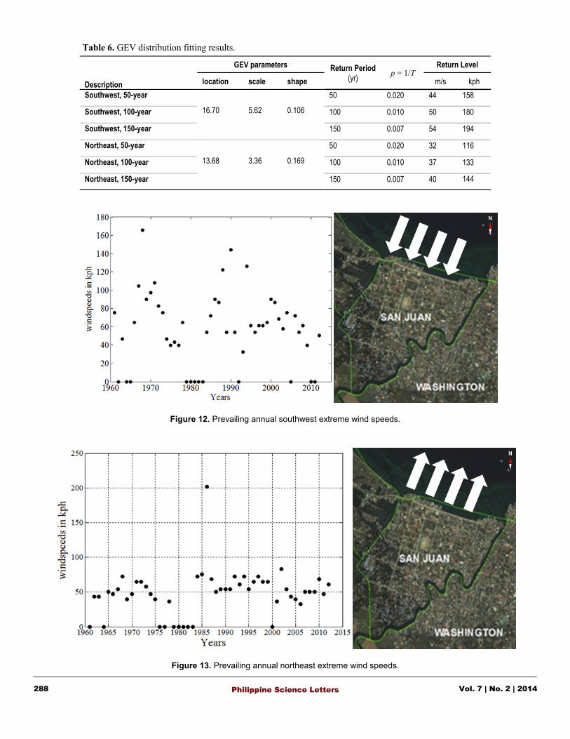
Table 6. GEV distribution fitting results.


Description

GEV parameters Return Period

(yr) p = 1/T

Return Level

location scale shape m/s kph

Southwest, 50-year

16.70

5.62

0.106

50 0.020 44 158

Southwest, 100-year 100 0.010 50 180

Southwest, 150-year 150 0.007 54 194

Northeast, 50-year

13.68

3.36

0.169

50 0.020 32 116

Northeast, 100-year 100 0.010 37 133

Northeast, 150-year 150 0.007 40 144

Figure 12. Prevailing annual southwest extreme wind speeds.

Figure 13. Prevailing annual northeast extreme wind speeds.


Group No

Case

Wind speed (kph) F-value F-critical

unobstructed theoretical actual

2,1,1 1st row shielding 2nd row

group 1

4.5 4.05 4.30

0.0225 7.709 2.6 2.34 2.10

2.8 2.52 2.10

2,1,2

1st row shielding 2nd row

group 2

4.5 3.96 2.10

0.926 7.709 1.6 1.41 1.10

1.7 1.58 1.20

1,1,3

1st row shielding 2nd row

group 3

3.1 2.86 2.20

30.962 5.987 2.8 2.58 2.30

2.9 2.67 2.30

3.2 2.95 2.10

2,2,1

2nd row shielding 3rd row

group 1

3.7 3.23 2.20

6.417 7.709 3.0 2.62 2.20

2.9 2.53 2.30

2,2,2


group 2

1.5 1.49 1.30

0.074 7.709 0.9 0.89 0.80

0.6 0.59 0.60

1,2,3


group 3

0.70 0.61 0.80

0.941 5.987 1.60 1.40 1.20

1.00 0.87 0.90

0.50 0.44 0.50

Table 7. Observed 10-minute average wind speeds.

(A) Unshielded condition (B) Shielded condition

Figure 14. Site observation of wind speeds.


Hazard maps

The hazard map also takes into account two directions and

three levels of return period each. These maps were developed

using ordinary Kriging as the method for spatial analysis. An

increment of 20 kph of wind was used to divide the map into

different zones denoted by different colors. A visible reduction

of wind speed per distance can be observed due to the effects of

shielding. This is not to say, however, that with a sufficient

number of houses the wind effect would be null. Two direc-

tions should always be considered when determining the hazard

of the specific point, and the higher wind speed value should

govern.

CONCLUSION

Six different contour and hazard maps were developed

using ArcGIS for barangay San Juan, Surigao City, Surigao del

Norte. This method promises acceptable results since it takes

into account historical, analytical, and experimental methods in

determining the hazard of wind. Extreme wind speed data gath-

ered by the Surigao PAGASA station were fitted to a GEV

distribution. To validate the simulated values, wind data were

gathered at the site to support the shielding effect correction

factor.

It is recommended that long-term gathering of wind data

(10-minute and 3-second wind speeds) is needed to further im-

prove the GEV distribution inference. These data can also be

used for reliability studies (of vulnerable structures) and to

validate the probability of failure estimates of low-cost and low

-rise residential structures after an extreme wind event.

ACKNOWLEDGEMENTS

The authors wish to acknowledge Professor Sharag-Eldin

for the fruitful e-mail exchange regarding the correction factor

used in this study, Mr. Abel Tejo of Surigao del Norte Land

Use and Planning Department for the assistance in the data

gathering, and PAGASA (Manila and Surigao office) for the

extreme wind speed data used in this study.

CONFLICTS OF INTEREST

There are no conflicts of interest.

CONTRIBUTION OF INDIVIDUAL AUTHORS

Marvin Salazar is the main author of this research. This

research is part of his undergraduate thesis at the Civil Engi-

neering Department of De La Salle University - Manila. Les-

sandro Garciano proposed the idea, revised and reviewed the

paper in its final form. He is also the adviser of the first author

in his undergraduate thesis.

Figure 15. Locations where the wind speeds were observed.


(A) 50-year (B) 100-year (C) 150-year

Figure 16. Extreme wind speed contour maps (NE direction).


Figure 17. Extreme wind speed contour maps (SW direction).


Figure 18. Extreme wind speed hazard maps (NE direction).


Figure 19. Extreme wind speed hazard maps (SW direction).


REFERENCES

Alonzo A. “’Sendong’ among deadliest cyclones to enter PHL

in 12 years”. Available: http://www.gmanetwork.com/

news/story/242058/news/nation/sendong-among-

deadliest-cyclones-to-enter-phl-in-12-years. GMA news

online 2011: (Accessed on March 7, 2014).

ANC (ABS-CBN News Channel). Pablo tears up roofs in Suri-

gao; blackouts remain. Retrieved from http://www.abs-

cbnnews.com/video/nation/regions/12/04/12/pablo-tears-

roofs-surigao-blackouts-remain. 2012: (Accessed on

March 7, 2014).

ASEP (Association of Structural Engineers of the Philippines).

National Structural Code of the Philippines, 6th edition,

Vol. 1, Quezon City, Philippines. 2010.

BBC News Asia. Dozens dead in Philippine floods. http://

news.bbc.co.uk/2/hi/asia-pacific/8276347.stm.

2009:(Accessed on April 10, 2014).

Coles S. An introduction to statistical modelling of extreme

values, Springer-Verlag, 2001.

CRED (Centre for Research on the Epidemiology of Disasters).

Emergency Events Database. http://www.emdat.be/

disaster-list. 2013: (Accessed on August 16, 2013).

De Leoz TB, Kaw ER, Quidilla A, Valbuena JG, Garciano LE.

Updating the wind zone map and developing contour

maps for the Philippines: Adaptation strategies for ex-

treme wind speeds. In Proceedings of the 4th ASEP Con-

vention on Concrete Engineering Practice and Technol-

ogy 2014; 13 pages.

Garciano LE, Hoshiya M, Maruyama O. Development of a

regional map of extreme wind speeds in the Philippines.

JSCE Journal of Structural Eng / Earthquake Eng 2005;

22(1): 21-32.

Kennedy M. Introducing Geographic Information systems with

ArcGIS: A Workbook Approach to learning GIS. 2nd

edition: John Wiley & Sons, 2009.

Legaspi A. Typhoon pablo is strongest storm to hit Mindanao

in two decades. http://www.gmanetwork.com/news/

story/284922/news/nation/typhoon-pablo-is-strongest-

storm-to-hit-mindanao-in-two-decades. GMA NEWS

Network: 2012 (Accessed on April 10, 2014).

NDRRMC (National Disaster Risk Reduction and Management

Council). Effects of Typhoon Yolanda. 2013.

NDRRMC (National Disaster Risk Reduction and Management

Council). Situation report on the effects of typhoon

Pablo. 2012.

Pacheco BM, Tanzo WT, Aquino RE. Recent Wind Engineer-

ing Developments in the Philippines: 2007 - 2009. In

Proceedings of the 5th Workshop on Regional Harmoni-

zation of Wind Loading and Wind Environmental Speci-

fications in Asia-Pacific Economies. Taiwan: 2009.

Salazar MA. A methodology for site-specific wind contouring

and hazard mapping: A case study in Surigao City. Un-

dergraduate thesis of the Department of Civil Engineer-

ing, De La Salle University 2014; 85 pages.

Sharag-Eldin A. A parametric model for predicting wind-

induced pressures on low-rise vertical surfaces in

shielded environments. Solar Energy 2007; 81: 52-61.

Vickery PJ, Masters FJ, Powell MD, Wadhera D. Ultimate

wind load design gust wind speed in the United States

for use in ASCE-7. Journal of Structural Engineering

2010; 136(5): 613-625.

Zar JH. Biostatistical Analysis. 2nd ed. Englewood Cliffs, NJ:

Prentice-Hall, Inc, 1984.

Probabilistic wind contouring and hazard mapping of ...philsciletters.org/2014/PSL...

Documents

Transcript of Probabilistic wind contouring and hazard mapping of ...philsciletters.org/2014/PSL...