J Intell Inf SystDOI 10.1007/s10844-010-0141-4

Probabilistic skylines on uncertain data: modeland bounding-pruning-refining methods

Bin Jiang · Jian Pei · Xuemin Lin · Yidong Yuan

Received: 29 November 2009 / Revised: 5 November 2010 / Accepted: 9 November 2010© Springer Science+Business Media, LLC 2010

Abstract Uncertain data are inherent in some important applications. Although aconsiderable amount of research has been dedicated to modeling uncertain dataand answering some types of queries on uncertain data, how to conduct advancedanalysis on uncertain data remains an open problem at large. In this paper, we tacklethe problem of skyline analysis on uncertain data. We propose a novel probabilisticskyline model where an uncertain object may take a probability to be in the skyline,and a p-skyline contains all objects whose skyline probabilities are at least p (0 <

p ≤ 1). Computing probabilistic skylines on large uncertain data sets is challenging.We develop a bounding-pruning-refining framework and three algorithms systemat-ically. The bottom-up algorithm computes the skyline probabilities of some selectedinstances of uncertain objects, and uses those instances to prune other instancesand uncertain objects effectively. The top-down algorithm recursively partitionsthe instances of uncertain objects into subsets, and prunes subsets and objects

This research is supported in part by an NSERC Discovery Grant, an NSERC DiscoveryAccelerator Supplement Grant, the ARC Discovery Grants (DP110102937, DP0987557,DP0881035), and a Google research Award. All opinions, findings, conclusions andrecommendations in this paper are those of the authors and do not necessarilyreflect the views of the funding agencies.

B. Jiang (B) · J. PeiSchool of Computing Science, Simon Fraser University, Burnaby, BC, Canadae-mail: bjiang@cs.sfu.ca

J. Peie-mail: jpei@cs.sfu.ca

X. Lin · Y. YuanSchool of Computer Science and Engineering,The University of New South Wales and NICTA, Sydney, NSW, Australia

X. Line-mail: lxue@cse.unsw.edu.au

Y. Yuane-mail: yyidong@cse.unsw.edu.au

J Intell Inf Syst

aggressively. Combining the advantages of the bottom-up algorithm and the top-down algorithm, we develop a hybrid algorithm to further improve the performance.Our experimental results on both the real NBA player data set and the benchmarksynthetic data sets show that probabilistic skylines are interesting and useful, and ouralgorithms are efficient on large data sets.

Keywords Uncertain data · Skyline queries · Probabilistic queries · Algorithms

1 Introduction

Uncertain data are inherent in some important applications, such as environmentalsurveillance, market analysis, and quantitative economics research. Uncertain datain those applications are generally caused by factors like data randomness andincompleteness, limitations of measuring equipment, delayed data updates, etc.Due to the importance of those applications and the rapidly increasing amount ofuncertain data collected and accumulated, analyzing large collections of uncertaindata has become an important task. Although a considerable amount of research hasbeen dedicated to modeling uncertain data and answering some types of queries onuncertain data (please see Section 7 for a brief review), how to conduct advancedanalysis on uncertain data remains an open problem at large. Particularly in thisstudy, we will address the problem of skyline analysis.

1.1 Motivating examples

Many previous studies (e.g., Borzsonyi et al. 2001; Chan et al. 2006a; Huang et al.2006; Lin et al. 2005; Pei et al. 2005, 2007a; Sharifzadeh and Shahabi 2006; Tao et al.2006; Yuan et al. 2005) showed that skyline analysis is very useful in multi-criteriadecision making applications. As an example, consider analyzing NBA players usingmultiple technical statistics criteria (e.g., the number of assists and the number ofrebounds). Ideally, we want to find the perfect player who can achieve the bestperformance in all aspects. Such a player, however, does not exist. The skylineanalysis here is meaningful since it discloses the tradeoff among the merits of multipleaspects.

A player U is in the skyline if there exists no other player V such that V is betterthan U in one aspect, and is not worse than U in all other aspects. Skyline analysis onthe technical statistics data of NBA players can identify excellent players and theiroutstanding merits.

We argue that skyline analysis is also meaningful on uncertain data. Consider theskyline analysis on NBA players again. Since the annual statistics are used as certaindata in previous studies (Pei et al. 2005), it has never been addressed in the skylineanalysis that players may have different performances in different games. If the game-by-game performance data are considered, which players should be in the skyline andwhy?

For example, let us use the number of assists and the number of rebounds, both thelarger the better, to examine the players. The two measures may vary substantiallyplayer by player and game by game. Uncertainty is inherent due to many factors suchas the fluctuations of players’ conditions, the locations of the games, and the supportfrom audience. How can we def ine the skyline given the uncertain data?

J Intell Inf Syst

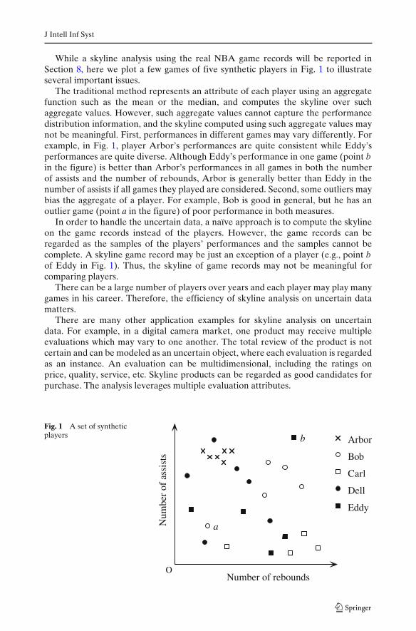
While a skyline analysis using the real NBA game records will be reported inSection 8, here we plot a few games of five synthetic players in Fig. 1 to illustrateseveral important issues.

The traditional method represents an attribute of each player using an aggregatefunction such as the mean or the median, and computes the skyline over suchaggregate values. However, such aggregate values cannot capture the performancedistribution information, and the skyline computed using such aggregate values maynot be meaningful. First, performances in different games may vary differently. Forexample, in Fig. 1, player Arbor’s performances are quite consistent while Eddy’sperformances are quite diverse. Although Eddy’s performance in one game (point bin the figure) is better than Arbor’s performances in all games in both the numberof assists and the number of rebounds, Arbor is generally better than Eddy in thenumber of assists if all games they played are considered. Second, some outliers maybias the aggregate of a player. For example, Bob is good in general, but he has anoutlier game (point a in the figure) of poor performance in both measures.

In order to handle the uncertain data, a naïve approach is to compute the skylineon the game records instead of the players. However, the game records can beregarded as the samples of the players’ performances and the samples cannot becomplete. A skyline game record may be just an exception of a player (e.g., point bof Eddy in Fig. 1). Thus, the skyline of game records may not be meaningful forcomparing players.

There can be a large number of players over years and each player may play manygames in his career. Therefore, the efficiency of skyline analysis on uncertain datamatters.

There are many other application examples for skyline analysis on uncertaindata. For example, in a digital camera market, one product may receive multipleevaluations which may vary to one another. The total review of the product is notcertain and can be modeled as an uncertain object, where each evaluation is regardedas an instance. An evaluation can be multidimensional, including the ratings onprice, quality, service, etc. Skyline products can be regarded as good candidates forpurchase. The analysis leverages multiple evaluation attributes.

Fig. 1 A set of syntheticplayers

Num

ber

of a

ssis

ts

Number of reboundsO

Arbor

Bob

Carl

Dell

Eddy

b

a

J Intell Inf Syst

To evaluate the effect of therapies in medical practice, test cases are collected,and a few measures are used. Generally, the measures may vary, sometimes evensubstantially, among the test cases of one therapy. Uncertainty is inherent due to theincompleteness of the samples and many other factors (e.g., the physical conditionsof patients). Finding the skyline therapies on the uncertain data helps to identifygood therapies and understand the tradeoff among multiple factors in question.

As one more example, consider damage control of typhoons (or hurricanes).Tens of thousands of automatic observation stations can be deployed in the areaaffected by typhoons to collect data like wind intensity and precipitation. A locationis likely more seriously damaged if its wind intensity and precipitation are both largeunder a typhoon attack. However, there are more than ten typhoons every year,and each typhoon takes a different route. Thus, it will be useful to model a locationas an uncertain object and the wind intensity and precipitation as the attributes.When a location is affected by a typhoon, the data are recorded as an occurrenceof the uncertain object. Based on the data, we can analyze the most likely seriouslydamaged locations.

In summary, uncertain data pose a few new challenges for skyline analysis andcomputation. Specifically, we need a meaningful yet simple model for skylines onuncertain data. Moreover, we need to develop efficient algorithms for such skylinecomputation.

1.2 Challenges and our contributions

In this paper, we address two major challenges about skyline analysis and computa-tion on uncertain data.

1.2.1 Challenge 1: modeling skylines on uncertain data

In a set of uncertain objects, each object has multiple instances, or alternatively, eachobject is associated with a probability density function. A model about skylines onuncertain data needs to answer two questions:

– How can we capture the dominance relation between uncertain objects?– What should be the skyline on those uncertain objects?

Our contributions We introduce the probabilistic nature of uncertain objects intothe skyline analysis. We follow the possible world model (Abiteboul et al. 1987;Imielinski and Witold Lipski 1984; Sarma et al. 2006) which has been adoptedextensively in recent studies on uncertain data processing, such as Soliman et al.(2007), Benjelloun et al. (2006) and Burdick et al. (2005).

Essentially, to compare the advantages between two objects, we calculate theprobability that one object dominates the other. Based on the probabilistic domi-nance relation, we propose the notion of probabilistic skyline. The probability of anobject being in the skyline is the probability that the object is not dominated by anyother objects.

Given a probability threshold p (0 ≤ p ≤ 1), the p-skyline is the set of uncertainobjects each of which takes a probability of at least p to be in the skyline.

J Intell Inf Syst

Comparing to the traditional skyline analysis, probabilistic skyline analysis is moreinformative on uncertain objects.

– First, traditional skylines, computed either using aggregates or individual in-stances, can be biased by outliers and do not consider the distribution of theinstances of an uncertain object. Probabilistic skylines, on the other hand, take allinstances of an object and their distribution together to determine the dominancerelationship, thus can provide more reliable results.

– Second, the size of the traditional skyline can be large when the data sethas a large cardinality or dimensionality (Chan et al. 2006a, c). Users cannotfurther compare objects in the skyline and have to turn to other analytical tools.This makes the result difficult to process. However, probabilistic skylines cannaturally rank objects according to their skyline probabilities. The size of the p-skyline can be controlled by tuning the probability threshold p. This provides amore user-friendly interaction to digest the results.

For example, in a case study (details in Section 8) using the game-by-gametechnical statistics of 1,313 NBA players in 339,721 games, the traditional skylinecomputed on average player statistics has 20 players. By contrast, the 0.3-skylineincludes five players, the 0.2-skyline includes 14 players, and the 0.1-skyline includes42 players. Among them, some players that have relatively high skyline probabilities,such as Hakeem Olajuwon (0.204) and Kobe Bryant (0.2), are not in the traditionalskyline where only the aggregate statistics are used. On the other hand, some playersthat are in the traditional skyline have a low skyline probability, such as Gary Payton(0.126) and Lamar Odom (0.102). These are due to their biased game records.We will provide more explanation in Section 8. Clearly, this information cannot beobtained using the traditional skyline analysis.

To the best of our knowledge, we are the first to study skyline analysis onuncertain objects.

1.2.2 Challenge 2: ef f icient computation of probabilistic skylines

Computing a probabilistic skyline is much more complicated than computing askyline on certain data. Particularly, in many applications, the probability densityfunction of an uncertain object is often unavailable explicitly. Instead, a set ofinstances are collected in the hope of approximating the probability density function.According to the possible world model, the probabilistic skyline should be derivedfrom an exponential number of possible worlds. Thus, it is challenging to computeprobabilistic skylines on uncertain objects, each of which is represented by a set ofinstances.

In this paper, we focus on the discrete case of probabilistic skylines computation,i.e., each uncertain object is represented by a set of instances. There are severalchallenges associated with computing probabilistic skylines in the discrete case. First,each uncertain object may have many instances to be processed. Second, we have toconsider many probabilities in deriving the probabilistic skylines. For example, asreported in Section 8, a straightforward method takes more than 1 h to computethe 0.3-skyline on the NBA data set. Using the techniques developed in this paper,we are able to compute probabilistic skylines efficiently and outperform exhaustivesearch methods by orders of magnitude.

J Intell Inf Syst

Our contributions We develop a bounding-pruning-refining framework. As theimplementation of the framework, we devise three algorithms to tackle the problem.

– The bottom-up algorithm computes the skyline probabilities of some selectedinstances of uncertain objects, and uses those instances to prune other instancesand uncertain objects effectively.

– The top-down algorithm recursively partitions the instances of uncertain objectsinto subsets, and prunes subsets and objects aggressively.

– Combining the advantages of the bottom-up algorithm and the top-down algo-rithm, we develop a hybrid algorithm to further improve the performance. Wegreedily assign objects to the bottom-up method or the top-down method forprocessing according to the distribution of the instances and the relationship withrespect to other objects.

Our methods are efficient and scalable. As verified by our extensive experimentalresults, our methods are at least one order of magnitude faster than the exhaustivemethod.

1.2.3 Paper organization

The rest of the paper is organized as follows. In Section 2, we propose the modelof probabilistic skylines on uncertain data. In Section 3, we propose the bounding-pruning-refining framework. The bottom-up method and the top-down methodare developed in Sections 4 and 5, respectively. We devise the hybrid method inSection 6. We review the related work in Section 7. A systematic performance studyis reported in Section 8. We conclude the paper in Section 9.

2 Probabilistic skylines

In this section, we present the probabilistic skyline model. For reference, a summaryof notations is given in Table 1.

We first recall the notions of the dominance relation and skylines on certainobjects. Then, we extend the dominance relation to probabilistic dominance relationon uncertain objects. Last, we extend the skylines on certain objects to probabilisticskylines on uncertain objects.

Table 1 The summary ofnotations

Notation Definition

U , V Uncertain objectsu, v Instances of uncertain objects|U | The number of instances of UfU The probability density function of Upu The probability of u to appearPr[U ≺ V] The probability that U dominates VPr(·) Skyline probability of U or uPr+(·) The upper bound of Pr(U) or Pr(u)

Pr−(·) The lower bound of Pr(U) or Pr(u)

U.MBB The minimum bounding box of UUmax(Umin) The upper (lower) corner of U.MBB

J Intell Inf Syst

2.1 Skylines on certain objects

By default, we consider points in an n-dimensional numeric space D = (D1, . . . , Dn).The dominance relation is built on the preferences in attributes D1, . . . , Dn. Withoutloss of generality, we assume that, on D1, . . . , Dn, smaller values are more preferable.

For two points u and v, u is said to dominate v, denoted by u ≺ v, if for everydimension Di (1 ≤ i ≤ n), u.Di ≤ v.Di, and there exists a dimension Di0 (1 ≤ i0 ≤ n)

such that u.Di0 < v.Di0 .Given a set of points S, a point u ∈ S is a skyline point if there exists no other point

v ∈ S such that v dominates u. The skyline on S is the set of all skyline points.

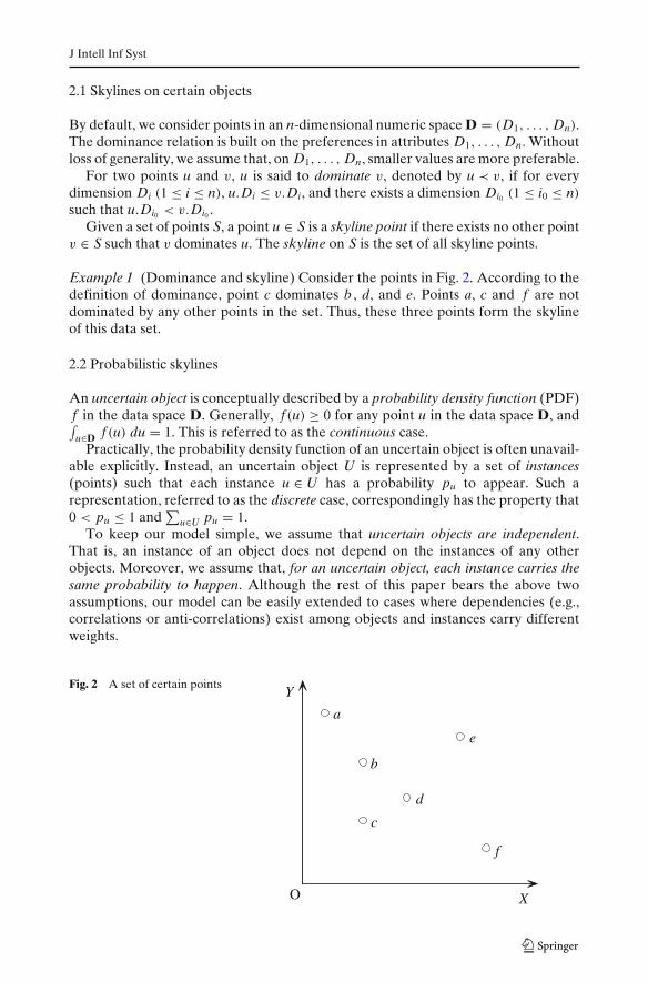
Example 1 (Dominance and skyline) Consider the points in Fig. 2. According to thedefinition of dominance, point c dominates b , d, and e. Points a, c and f are notdominated by any other points in the set. Thus, these three points form the skylineof this data set.

2.2 Probabilistic skylines

An uncertain object is conceptually described by a probability density function (PDF)f in the data space D. Generally, f (u) ≥ 0 for any point u in the data space D, and∫u∈D f (u) du = 1. This is referred to as the continuous case.

Practically, the probability density function of an uncertain object is often unavail-able explicitly. Instead, an uncertain object U is represented by a set of instances(points) such that each instance u ∈ U has a probability pu to appear. Such arepresentation, referred to as the discrete case, correspondingly has the property that0 < pu ≤ 1 and

∑u∈U pu = 1.

To keep our model simple, we assume that uncertain objects are independent.That is, an instance of an object does not depend on the instances of any otherobjects. Moreover, we assume that, for an uncertain object, each instance carries thesame probability to happen. Although the rest of this paper bears the above twoassumptions, our model can be easily extended to cases where dependencies (e.g.,correlations or anti-correlations) exist among objects and instances carry differentweights.

Fig. 2 A set of certain points

a

e

c

b

f

d

Y

XO

J Intell Inf Syst

Now, let us extend the dominance relation to uncertain objects, and show how thiscan straightforwardly define skylines on uncertain objects.

Let U and V be two uncertain objects, and fU and fV be the correspondingprobability density functions, respectively. Then, the probability that V dominatesU is

Pr[V ≺ U] =∫

u∈DfU (u)

(∫

v≺ufV(v) dv

)

du

=∫

u∈D

∫

v≺ufU (u) fV(v) dvdu (1)

In the discrete case, the probability that V dominates U is given by

Pr[V ≺ U] =∑

u∈U

pu ·⎛

⎝∑

v∈V,v≺u

pv

⎞

⎠ (2)

Since any two points u and v in the data space must have one of the following threerelations: u ≺ v, v ≺ u, or u and v do not dominate each other, for two uncertainobjects U and V, Pr[U ≺ V] + Pr[V ≺ U] ≤ 1.

Example 2 (Probabilistic dominance relation) Consider the set of three uncertainobjects in Fig. 3. Each object has two instances. Assume each instance takes equalprobability to appear, that is, the appearance probability of each instance is 0.5.

For instances of object C, c1 is dominated by every instance of A, and c2 isdominated by instance a2 of A. Thus, the probability that A dominates C is Pr[A ≺C] = 0.5 × 1 + 0.5 × 0.5 = 0.75. Similarly, we can calculate Pr[B ≺ C] = 0.5.

Since c1 is dominated by every instance of object A and c2 is dominated by everyinstance of object B, the probability that C is dominated by A or B is 1. In otherwords, C cannot be in the skyline.

Because Pr[A ≺ C] and Pr[B ≺ C] are not independent, an important obser-vation here is that, although Pr[A ≺ C] = 0.75 < 1 and Pr[B ≺ C] = 0.5 < 1, theprobability of C being dominated by A or B is 1. Moreover, Pr[(A �≺ C) ∧ (B �≺C)] �= (1 − Pr[A ≺ C]) · (1 − Pr[B ≺ C]).

Fig. 3 A set of uncertainobjects

a1

a2b2

b1

c1

c2

Object A

Object B

Object C

Y

XO

J Intell Inf Syst

The observation in Example 2 indicates that the probabilistic dominance relationsare not independent and cannot be used straightforwardly to def ine skylines onuncertain objects. Then, what is the probability that an uncertain object is in theskyline?

We first illustrate our probabilistic skyline model in the discrete case. Then weshow the model in the continuous case.

Given a set of uncertain objects S = {U1, · · · , Um}, a possible world w ={u1, · · · , um} is a set of m instances such that each uncertain object in S has oneinstance in w. The probability of w to appear is

Pr(w) =m∏

i=1

pui .

Let � be the set of all possible worlds, then∑

w∈�

Pr(w) = 1.

Let Sky(w) denote the set of objects such that for every object U ∈ Sky(w), theinstance of U in w is in the skyline of w. Then, the probability that U appears in theskylines of the possible worlds is

Pr(U) =∑

U∈Sky(w),w∈�

Pr(w).

Pr(U) is called the skyline probability of U .

Example 3 (Probabilistic skylines) Consider the set of uncertain objects in Fig. 3again. We have eight possible worlds in total. Each possible world has the probability0.53 = 0.125 to appear.

P(A) = 1 since a1 and a2 are in the skyline of every possible world. Moreover,P(C) = 0 because c1 and c2 are not in the skyline of any possible world.

Note that B is in the skylines of four possible worlds {a1, b 1, c1}, {a1, b 1, c2},{a1, b 2, c1}, and {a1, b 2, c2}. Therefore, P(B) = 4 × 0.125 = 0.5.

For each instance u of U ∈ S, Pr(u), the probability of u being in the skyline, is

Pr(u) =∏

V∈S\{U}

⎛

⎝1 −∑

v∈V,v≺u

pv

⎞

⎠ . (3)

Pr(u) is called the skyline probability of instance u.By the above definition, it can be immediately verified that

Pr(U) =∑

u∈U

pu · Pr(u). (4)

Consequently, we have

P(U) =∑

u∈U

pu · Pr(u) =∑

u∈U

⎛

⎝pu ·∏

V∈S\{U}

⎛

⎝1 −∑

v∈V,v≺u

pv

⎞

⎠

⎞

⎠ . (5)

J Intell Inf Syst

Similarly, in the continuous case, the skyline probability Pr(U) is defined as

Pr(U) =∫

u∈DfU (u)

∏

V �=U

(

1 −∫

v≺ufV(v) dv

)

du. (6)

An uncertain object may take a probability to be in the skyline. It is natural toextend the notion of skyline to probabilistic skyline. For a set of uncertain objects Sand a probability threshold p (0 ≤ p ≤ 1), the p-skyline is the subset of objects in Seach of which takes a probability of at least p to be in the skyline. That is,

Sky(p) = {U ∈ S|Pr(U) ≥ p}.

Problem Definition 1 Given a set of uncertain objects S and a probability thresholdp (0 ≤ p ≤ 1), the problem of probabilistic skyline computation is to compute thep-skyline on S.

Particularly, in this paper, we tackle the discrete case problem. That is, given a setof uncertain objects where each object is a set of sample instances and a probabilitythreshold p, compute the p-skyline.

Although we will focus on the discrete case in this paper, some of our ideas canbe applied to handle the continuous case, which will be discussed briefly in Section 9.Moreover, we only address the exact algorithms in this paper. The developmentof approximation algorithms for probabilistic skylines is very interesting and isinvestigated systematically in another study we are conducting.

3 The bounding-pruning-refining framework

On a large uncertain data set, the number of possible worlds can be huge. Forexample, consider a data set of 1,000 uncertain objects. If each uncertain object hasfour instances, the number of possible worlds |�| = 41,000 > 10602. It is impracticalto compute the skylines in all possible worlds one by one and derive the skylineprobability for each uncertain object.

To tackle the problem, we propose a bounding-pruning-refining framework. Aprobabilistic skyline computation method can conduct iterations in the followingthree steps.

Bounding For an uncertain object U , we try to obtain an upper bound and a lowerbound on the skyline probability of U . This can be achieved by, forexample, computing the skyline probabilities of some selected instancesof U , or partitioning U into some subsets where the skyline probabilityof each subset can be bounded.

Pruning For an uncertain object U , if the lower bound of Pr(U) is larger than orequal to p, the probability threshold, then U is in the p-skyline. If theupper bound of Pr(U) is smaller than p, then U is not in the p-skyline.In both cases, we do not need to compute the skyline probabilities ofinstances in U anymore.

Refining If p is between the lower bound and the upper bound of Pr(U), thenwe need to get tighter bounds of the skyline probabilities by the nextiteration of bounding, pruning and refining.

J Intell Inf Syst

The above iteration goes on until for every uncertain object we can determinewhether it is in the p-skyline or not.

In the next two sections, we will propose two methods implementing the abovebounding-pruning-refining framework. The two methods differ in how to computeand refine the bounds and how to prune uncertain objects. The bottom-up method isdescribed in Section 4 and the top-down method is presented in Section 5.

4 The bottom-up method

In the bottom-up method, in the bounding step, we compute the skyline probabilitiesof a small subset of instances. In the pruning step, an uncertain object may be prunedusing the skyline probabilities of its instances, or those of some other objects. Themethod is called bottom-up since the bound computation and refinement start fromthe instance level (bottom) and go up to the object level.

4.1 Bounding skyline probabilities

Given an uncertain object U and an instance u of U , trivially, we have 0 ≤ Pr(U) ≤ 1and 0 ≤ Pr(u) ≤ 1. Let

Umin =( |U |

mini=1

{ui.D1}, . . . ,|U |

mini=1

{ui.Dn})

and

Umax =(

|U |maxi=1

{ui.D1}, . . . , |U |maxi=1

{ui.Dn})

be the minimum and the maximum corners of the minimum bounding box (MBBfor short) of U , respectively. Note that, Umin and Umax are not necessary two actualinstances of U . In this case, we treat them as virtual instances and define their skylineprobabilities following (3). That is,

Pr(Umin) =∏

V �=U

(

1 − |{v ∈ V | v ≺ Umin}||V|

)

, and

Pr(Umax) =∏

V �=U

(

1 − |{v ∈ V | v ≺ Umax}||V|

)

.

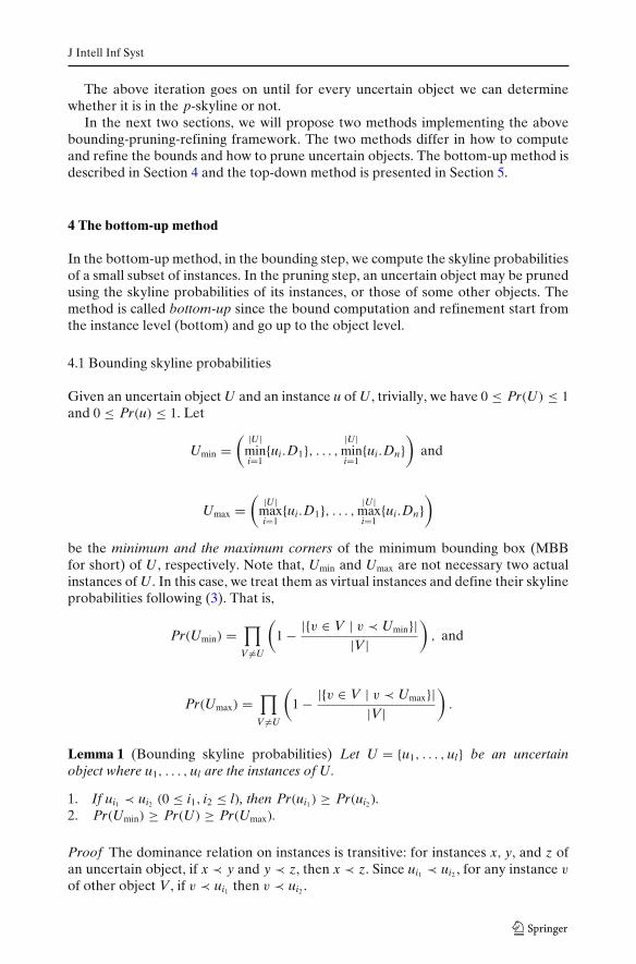
Lemma 1 (Bounding skyline probabilities) Let U = {u1, . . . , ul} be an uncertainobject where u1, . . . , ul are the instances of U.

1. If ui1 ≺ ui2 (0 ≤ i1, i2 ≤ l), then Pr(ui1) ≥ Pr(ui2).2. Pr(Umin) ≥ Pr(U) ≥ Pr(Umax).

Proof The dominance relation on instances is transitive: for instances x, y, and z ofan uncertain object, if x ≺ y and y ≺ z, then x ≺ z. Since ui1 ≺ ui2 , for any instance v

of other object V, if v ≺ ui1 then v ≺ ui2 .

J Intell Inf Syst

Applying the transitivity to (3), we have

Pr(ui1) =∏

V �=U

(

1 − |{v ∈ V | v ≺ ui1}||V|

)

≥∏

V �=U

(

1 − |{v ∈ V | v ≺ ui2}||V|

)

= Pr(ui2)

The first item in the lemma is proved.According to item 1 in this lemma, for any ui (1 ≤ i ≤ l), Pr(Umin) ≥ Pr(ui) ≥

Pr(Umax). Item 2 in the lemma follows with the above inequality and (4). �

Lemma 1 provides a means to compute the upper bounds and the lower boundsof instances and uncertain objects using the skyline probabilities of other instances.

According to the first inequality in the lemma, the skyline probability of aninstance can be bounded by those of other instances dominating or dominated by it.In other words, when the skyline probability of an instance is calculated, the boundsof the skyline probabilities of some other instances of the same object may be refinedaccordingly.

The second inequality in the lemma indicates that the minimum and the maximumcorners of the MBB can play important roles in bounding the skyline probability ofa set of instances.

4.2 Pruning techniques

If the skyline probability of an uncertain object or an instance of an uncertain objectis computed, can we use this information to prune the other uncertain instancesor objects? Following with Lemma 1, we immediately have the following rule todetermine the p-skyline membership of an uncertain object using its minimum ormaximum corners.

Pruning Rule 1 For an uncertain object U and probability threshold p, if Pr(Umin) <

p, then U is not in the p-skyline. If Pr(Umax) ≥ p, then U is in the p-skyline.

Moreover, we can prune an uncertain object using the upper bounds and the lowerbounds of the skyline probabilities of instances.

Pruning Rule 2 Let U be an uncertain object. For each instance u ∈ U, let Pr+(u)

and Pr−(u) be the upper bound and the lower bound of Pr(u), respectively. If1

|U |∑

u∈U Pr+(u) < p, then U is not in the p-skyline. If 1|U |

∑u∈U Pr−(u) ≥ p, then

U is in the p-skyline.

We can also use the information about one uncertain object to prune otheruncertain instances or objects. First, if an instance u of an uncertain object U isdominated by the maximum corner of another uncertain object V, then u can neverbe in the skyline in any possible world. Figure 4 illustrates this pruning rule.

Pruning Rule 3 Let U and V be uncertain objects such that U �= V. If u is an instanceof U and Vmax ≺ u, then Pr(u) = 0.

By pruning some instances in an uncertain object using the above rule, we canreduce the cost of computing the skyline probability of the object.

J Intell Inf Syst

Fig. 4 An illustration ofPruning Rule 3

U u

V

Vmax

When the skyline probabilities of some instances of an uncertain object arecomputed, we can use the information to prune some other uncertain objects.

Pruning Rule 4 Let U and V be two uncertain objects and U ′ ⊆ U be a subset ofinstances of U such that U ′

max � Vmin. If

|U − U ′||U | · min

u∈U ′{Pr(u)} < p,

then Pr(V) < p and thus V is not in the p-skyline.

Proof Figure 5 illustrates the situation. Since Vmin is dominated by all instances in U ′.An instance of V can be in the skyline only if U does not appear as any instance inU ′. Even if no instance in (U − U ′) dominates any instance of V, the probability thatV is in the skyline still cannot reach the probability threshold p, since U ′

max � Vmin

and |U−U ′ ||U | · minu∈U ′ {Pr(u)} < p. Thus V cannot be in the p-skyline.

Formally, since every instance of V is dominated by all instances in U ′, only whenU takes an instance in (U − U ′), V may have a chance of not being dominated by U .The probability that an instance of V is not dominated by an instance of U cannot be

Fig. 5 An illustration ofPruning Rule 4

U

V

U'max

Vmin

U'

J Intell Inf Syst

more than (1 − |U ′ ||U | ) = |U−U ′ |

|U | . Moreover, since U ′max � Vmin, all instances of objects

other than U and V dominating U ′max also dominate Vmin.

Thus,

Pr(V) ≤ Pr(Vmin) ≤(

1 − |U ′||U |

)

· Pr(U ′max) = |U − U ′|

U· Pr(U ′

max)

≤ |U − U ′|U

· minu∈U ′{Pr(u)} < p

V is not in the p-skyline. �

As a special case of Pruning Rule 4, if there exists an instance u ∈ U such thatPr(u) < p and u � Vmin, then Pr(V) < p and V can be pruned.

The pruning rule is powerful since even an uncertain object partially computedcan be used to prune other objects.

4.3 Refinement strategies

For an uncertain object U , we want to determine whether U is in the p-skyline bycomputing the skyline probabilities of as few instances of U as possible. Finding anoptimal subset of instances to compute is a very difficult online problem since, with-out computing the probabilities of the instances, we do not know their distribution.Here, we propose a layer-by-layer heuristic method.

4.3.1 Layers of instances

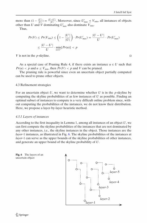
According to the first inequality in Lemma 1, among all instances of an object U , wecan first compute the skyline probabilities of the instances that are not dominated byany other instances, i.e., the skyline instances in the object. Those instances are thelayer-1 instances, as illustrated in Fig. 6. The skyline probabilities of the instances atlayer-1 can serve as the upper bounds of the skyline probabilities of other instances,and generate an upper bound of the skyline probability of U .

Fig. 6 The layers of anuncertain object

layer-1layer-2

layer-3

layer-4

layer-5

J Intell Inf Syst

If the upper bounds using the layer-1 instances are not enough to qualify ordisqualify U in the p-skyline, we need to refine the upper bounds. We can computethe skyline probabilities of the instances at layer-2 which are dominated only by theinstances at layer-1, as shown in Fig. 6, too. Similarly, we can partition the instancesof an object into layers.

Formally, for an uncertain object U , an instance u ∈ U is at layer-1 if u is notdominated by any other instance in U . An instance v is at layer-k (k > 1) if, v is notat the 1st, . . . , (k − 1)-th layers, and v is not dominated by any instances except forthose at the 1st, . . . , (k − 1)-th layers.

The advantage of partitioning instances of an object into layers is that, once theskyline probabilities of all instances at one layer are calculated, the probabilities canbe used as the upper bounds of the instances at the higher layers.

Lemma 2 In an uncertain object U, let u1,1, . . . , u1,l1 be the instances at layer-k1, andu2,1, . . . , u2,l2 be the instances at layer-k2, k1 < k2. Then, for any instance at layer-k2 u2, j2 (1 ≤ j2 ≤ l2), there exists an instance at layer-k1 u1, j1 (1 ≤ j1 ≤ l1) such that

Pr(u1, j1) ≥ Pr(u2, j2). Moreover,l1max

i=1{Pr(u1,i)} ≥ l2max

j=1{Pr(u2, j)}.

Proof Since k1 < k2, instance u2, j2 must be dominated by an instance at layer-k1.Otherwise, u2, j2 is at layer-k1 or some lower layer. Let u1, j1 be an instance at layer-k1 that dominates u2, j2 . Then, the first inequality follows with Lemma 1. The secondinequality follows with the first inequality. �

4.3.2 Partitioning instances to layers

How can instances of an object be assigned quickly into layers?For each instance u, we define the key of the instance as the sum of its values

in all attributes, that is, u.key =n∑

i=1

u.Di. Then, we sort all the instances in the key

ascending order. This is motivated by the SFS algorithm (Chomicki et al. 2003). Thesorted list of instances has a nice property: for instances u and v such that u ≺ v, uprecedes v in the sorted list.

We scan the sorted list once. The first instance has the minimum key value, and isassigned to layer-1. We compare the second instance with the first one. If the secondone is dominated, then it is assigned to layer-2; otherwise it is assigned to layer-1.

Generally, when we process an instance u, suppose at the time there already existh layers. We compare u with the instances currently at layer- h

2 �. One of the twocases may happen.

– If u is dominated by an instance at that layer, then u must be at some layer higherthan h

2 �.– Otherwise, u is neither dominated by, nor dominates, any instance at that layer.

Then, u must be at that layer or some lower layer.

We conduct this binary search recursively until u is assigned to a layer.Lemma 1 indicates that the minimum corner of the MBB of an uncertain object

leads to the upper bounds of the skyline probabilities of all instances as well as the

J Intell Inf Syst

object itself. As a special case, we assign this minimum corner as a virtual instance atlayer-0.

The above partitioning method has a nice property: all instances at a layer aresorted in the key ascending order.

4.3.3 Scheduling objects

From which objects should we start the skyline probability computation?In order to use the pruning rules discussed in Section 4.2 as much as possible, those

instances in uncertain objects that likely dominate many other objects or instancesshould be computed early. Heuristically, those instances which are close to the originmay have a better chance to dominate other objects and instances.

The instances of an uncertain object are processed layer by layer. Within eachlayer, the instances are processed in the key ascending order. As discussed inSection 4.2, some pruning rules enable us to use the partial information of someuncertain objects to prune other objects and instances, we interleave the processingof different objects.

Technically, all instances of an uncertain object are kept in a list. The minimumcorner of its MBB is treated as a special instance and put at the head of the list. Theheads of lists of all uncertain objects are organized into a heap. We iteratively processthe top instance in the heap. If an object cannot be pruned after its minimum corneris processed, we organize the rest of instances in its list in the layer and key valueascending order. Once an instance from an object is processed, the object sends thenext instance into the heap if its skyline membership is not determined. The properpruning rules are triggered if the conditions are satisfied.

4.4 Algorithm and implementation

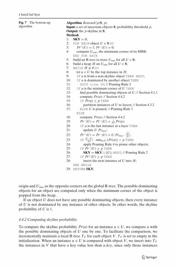
The bottom-up algorithm is shown in Fig. 7. We explain some critical implementationdetails here.

4.4.1 Finding possible dominating objects

For an object U , we want to find all the other objects that may contain some instancesdominating U . Those objects are called the possible dominating objects of U . Theskyline membership of U depends on only those possible dominating objects. Allother objects that do not contain any instances dominating U do not need to beconsidered.

To speed up the search of possible dominating objects, we employ R-trees (Guttman 1984). An R-tree is a tree data structure for indexing multidimen-sional data, such as points, etc. A node of an R-tree contains a set of entries. Eachentry at a leaf node is in the form of 〈pI D, coords〉 where pI D refers to the pointID and coords is the coordinates of the point. Each entry in a non-leaf node is in theform of 〈child, child.MBB〉 where child refers to a child node, and child.MBB is theminimum bounding box of all entries in this child node. Approximately, an R-treecan be built in time O(n log n) where n is the number of points indexed. A rangequery can be answered in time O(log n).

We organize the minimum corners of MBBs of all objects into a global R-tree.To find the possible dominating objects of U , we issue a window query with the

J Intell Inf Syst

Fig. 7 The bottom-upalgorithm

origin and Umax as the opposite corners on the global R-tree. The possible dominatingobjects for an object are computed only when the minimum corner of the object ispopped from the heap.

If an object U does not have any possible dominating objects, then every instanceof U is not dominated by any instance of other objects. In other words, the skylineprobability of U is 1.

4.4.2 Computing skyline probability

To compute the skyline probability Pr(u) for an instance u ∈ U , we compare u withthe possible dominating objects of U one by one. To facilitate the comparison, weincrementally maintain a local R-tree TV for each object V. TV is set to empty in theinitialization. When an instance u ∈ U is compared with object V, we insert into TV

the instances in V that have a key value less than u.key, since only those instances

J Intell Inf Syst

in V may dominate u. Then, we issue a window query with the origin and u as theopposite corners to compute |{v ∈ V|v ≺ u}|.

After comparing u with all possible dominating objects of U , using (4), we cancalculate Pr(u). We also update the lower bound of the probability of object Uimmediately as

Pr−(U) = Pr−(U) + 1|U | Pr(u).

Once all instances in a layer are processed, as discussed in Lemma 2, we usethe maximum probability of instances in this layer as the upper bound (denoted byU.Prmax) of the probabilities of instances in the higher layers. Moreover, the upperbound of the probability of U is updated as

Pr+(U) = Pr−(U) + U.Prmax · |U ||U | ,

where U ⊆ U is the set of instances whose probabilities are not calculated yet.

4.4.3 Using Pruning Rule 4

In order to use Pruning Rule 4 to prune other objects, for each object U , wemaintain U ′ as the set of instances which precede the current processing instancein its instance list. The skyline probability of those instances are already computed.Once U ′ satisfies the condition in the rule, we compute U ′

max, the maximum cornerof the MBB of U ′, and issue a window query on the global R-tree described inSection 4.4.1 with U ′

max and the maximum corner of the MBB of all objects in thedata set as the opposite corners. For each minimum corner returned from this query,the corresponding uncertain object satisfies the pruning rule and thus is not in the p-skyline. We note that for each object, this rule is applied at most once. This is becauseonce this condition is satisfied, it will be always satisfied afterwards.

4.5 Cost analysis of the bottom-up algorithm

It can be immediately verified that the cost of the bottom-up algorithm is pre-dominated by computing the skyline probabilities of instances as presented inSection 4.4.2. Suppose that R is the average cost of querying the local R-trees ofpossible dominating objects, with all pruning techniques are applied, for computingthe skyline probabilities of instances. Let Wtotal denote the number of instanceswhose skyline probabilities are computed in the algorithm. Then, the average costof the algorithm is O(Wtotal · R).

As shown in our experimental results, in practice many instances and objects canbe pruned sharply. The bottom-up algorithm only has to compute a small portion ofinstances. That is, Wtotal is much smaller than the total number of instances. Thus,the bottom-up algorithm has good scalability on the large data sets used in ourexperiments.

J Intell Inf Syst

5 The top-down method

In this section, we present a top-down method for probabilistic skyline computation.The method starts with the whole set of instances of an uncertain object. The skylineprobability of the object can be bounded using the maximum and the minimumcorners of the MBB of the object. To improve the bounds, we can recursivelypartition the instances into subsets. The skyline probability of each subset can bebounded using its MBB in the same way. Facilitated by (4), the skyline probability ofthe uncertain object can be bounded as the weighted mean of the bounds of subsets.Once the p-skyline membership of the uncertain object is determined, the recursivebounding process stops.

5.1 Partition trees

To facilitate the partitioning process, we use a partition tree data structure for eachuncertain object. A partition tree is binary. Each leaf node contains a set of instancesand the corresponding MBB. Each internal node maintains the MBB of all instancesin its descendants and the total number of instances.

The construction of a partition tree for an uncertain object is somewhat similar tothat of kd-trees (Bentley 1975). We start with a tree of only one node—the root nodewhich contains all instances of the object and the MBB. The tree grows in rounds. Ineach round, a leaf node with l instances (l > 1) is partitioned into two children nodesaccording to one attribute such that the left child and the right child contain l

2� and� l

2� instances, respectively.We take a simple round robin method to choose the attributes to grow a partition

tree. The attributes are sorted into D1, . . . , Dn in an arbitrary order. The root node(level-0) is partitioned into two children in attribute D1, those children (level-1) aresplit into grand-children in attribute D2, and so on. To split the nodes at level-n,attribute D1 is used again.

The time complexity to grow one level of the tree for an uncertain object U isO(|U |). The cost to fully grow a partition tree (i.e., each leaf node contains only oneinstance) is O(|U | log2 |U |) since the tree has at most log2 |U | levels.

5.2 Bounding using partition trees

For a node N in a partition tree, we also use N to denote the set of instances allocatedto N. Let N.MBB be the MBB of the instances allocated to N, and Nmax and Nmin

be the maximum and the minimum corners, respectively. Then, by Lemma 1, for anyinstance u ∈ N, the skyline probability of u can be bounded by

Pr(Nmax) ≤ Pr(u) ≤ Pr(Nmin). (7)

Moreover, if the partition tree of uncertain object U has l leaf nodes N1, . . . , Nl , then

1|U |

l∑

i=1

|Ni|·Pr(Ni,max)≤ Pr(U) ≤ 1|U |

l∑

i=1

|Ni|·Pr(Ni,min), (8)

where Ni,max and Ni,min are the maximum and the minimum corners of Ni.MBB,respectively, and |Ni| is the number of instances in Ni.

J Intell Inf Syst

Computing the exact skyline probabilities for all corners can be costly. Instead,we estimate the bounds. To bound the skyline probabilities for Nmin and Nmax for anode N in the partition tree of uncertain object U , we query the possible dominatingobjects of U as described in Section 4.4.1. We traverse the partition tree of eachpossible dominating object V of U in the depth-first manner. When a node M in thepartition tree of V is met, one of the following three cases happens.

– If Mmax dominates Nmin (as shown in Fig. 8a), then Nmin and Nmax are dominatedby all instances in M. That is, Pr(Nmin) ≤ Pr(Mmax).

– If Mmin does not dominate Nmax (as shown in Fig. 8b), then no instance in M candominate either Nmin or Nmax.

– If the above two situations do not happen, then some instances in M maydominate some instances in N (as shown in Fig. 8c). If M is an internal node, wetraverse the left and the right children of M recursively. Otherwise, M is a leafnode. Then, we estimate a lower bound of Pr(Nmax) by assuming all instances inM dominate Nmax, and an upper bound of Pr(Nmin) by assuming no instance inM dominates Nmin.

By traversing all partition trees of the possible dominating objects, we apply (3)to compute the upper bound for Pr(Nmin) and the lower bound for Pr(Nmax). Withthe two bounds and inequality (8), we can immediately bound the skyline probabilityof object U . We use only the maximum and the minimum corners of the MBBs, andnever compute the skyline probability of any one in a subset of instances.

5.3 Pruning and refinement using partition trees

When one level is grown for the partition trees of all uncertain objects whose skylinememberships are not determined, the possible dominating objects of them are alsopartitioned to the same level. For all new leaf nodes grown in this round, we boundtheir probabilities by traversing the partition trees of the corresponding possibledominating objects. We note that the computation of such bounding for the leafnodes which have the same MBB can be shared.

After that, we check whether some uncertain objects or some leaf nodes in somepartition trees may be pruned. That is, their skyline probabilities do not need to becomputed any more. Pruning those nodes can make the skyline computation faster.

M

N

Mmax

Nmin

(a)

M

NNmax

Mmin

(b)

M

N

(c)

Fig. 8 Three cases of bounding Pr(N)

J Intell Inf Syst

Consider a node N in the partition tree of uncertain object U . If there existsanother uncertain object V �= U such that Nmin is dominated by Vmax, then anyinstance in N cannot be in the skyline. In other words, Pr(u) = 0 for any u ∈ N. Wedo not need to compute any subset of N anymore since the instances there cannotcontribute to the skyline probability of U . Figure 9 illustrates this pruning rule.

Pruning Rule 5 Let N be a node in the partition tree of uncertain object U. If thereexists an object V �= U such that Vmax � Nmin, then node N can be pruned.

Moreover, if Pr(Nmin) = Pr(Nmax), according to inequality (7), the skyline proba-bility of any instance in N is determined. N can be pruned.

Pruning Rule 6 Let N be a node in the partition tree of uncertain object U. IfPr(Nmin) = Pr(Nmax), then for each u ∈ N, Pr(u) = Pr(Nmin) = Pr(Nmax) and nodeN can be pruned.

Last, once the skyline probability of an uncertain object can be bounded at leastp or less than p, then whether the object is in the p-skyline is determined. We do notneed to refine the estimation of the probability of this object anymore.

Pruning Rule 7 Let p be the probability threshold. Suppose the partition tree of anuncertain object U has l leaf nodes N1, . . . , Nl. Let Ni,max and Ni,min be the maximumand the minimum corners of Ni.MBB, respectively.

– If 1|U |

l∑

i=1

|Ni| · Pr(Ni,max) ≥ p, then U is in the p-skyline.

– If 1|U |

l∑

i=1

|Ni| · Pr(Ni,min) < p, then U is not in the p-skyline.

In both cases, the partition tree of U can be pruned.

Fig. 9 An illustration ofPruning Rule 5

U

Nmin

V

Vmax

N

J Intell Inf Syst

After the pruning step using the above rules, only the partition trees of thoseuncertain objects which cannot be determined in the p-skyline or not are left. Insuch trees, only those nodes whose skyline probabilities are not determined survive.

In a refinement step, we partition those surviving leaf nodes and their possibledominating objects to one more level. With the refinement, the bounds of skylineprobabilities are tighter.

5.4 The top-down algorithm and cost analysis

The top-down algorithm is shown in Fig. 10. In the implementation, we use an R-tree to index the minimum corners of the MBBs of all objects so that the search ofpossible dominating objects can be conducted efficiently.

Let P be the average cost of querying partition trees of possible dominatingobjects for bounding the skyline probabilities of the minimum and maximum cornersof MBBs, and Mtotal be the number of tree nodes whose skyline probabilities arebounded in the algorithm. Then, the average cost of the algorithm is O(Mtotal · P).

As will be shown in our experimental results, many nodes can be pruned sharplyby the pruning rules. The top-down algorithm only has to grow a small number of

Fig. 10 The top-downalgorithm

J Intell Inf Syst

tree nodes (i.e., Mtotal is small), and has good scalability with respect to cardinality ofthe data sets.

6 The hybrid method

In this section, we develop a hybrid method combining the advantages of the bottom-up method and the top-down method. The general idea is to partition the set S ofuncertain objects into two subsets SBU and ST D such that they likely can be processedby the bottom-up method and the top-down method efficiently, respectively.

In Section 6.1, we analyze the advantages and the disadvantages of the bottom-upmethod and the top-down method, and present the framework of the hybrid method.In Section 6.2, we discuss how to partition uncertain objects into two subsets SBU andST D. In Section 6.3, we apply the layer structure in the bottom-up method to improvethe top-down method.

6.1 The framework of the hybrid method

In our bounding-pruning-refining framework, we refine the upper bound and thelower bound of the skyline probability of every uncertain object. If the upper boundof the skyline probability of an uncertain object is less than p, the probabilitythreshold, the object is not in the p-skyline and thus can be pruned. If the lowerbound of the skyline probability of an uncertain object is at least p, the object is inthe p-skyline and can be removed from further refinement. Interestingly, the bottom-up method and the top-down method have different edges in bounding the skylineprobabilities of uncertain objects and pruning them.

The bottom-up method is good at pruning non-skyline objects. A non-skylineobject has a skyline probability smaller than the probability threshold. For a non-skyline object U , the bottom-up method can quickly obtain a tight upper boundof Pr(U) using the layer structure, since the instances in U having large skylineprobabilities are processed before those having small skyline probabilities. Once theupper bound of the skyline probability of U is determined lower than the probabilitythreshold, U can be pruned.

However, for a skyline object U ′, the lower bound of Pr(U ′) may not increase fastin the bottom-up method, since the lower bound is the sum of the skyline probabili-ties of the instances of U ′ processed so far. For example, if the probability thresholdp = 0.9 and every instance in an uncertain object U ′ takes the same probability toappear, in the bottom-up method, we have to process at least 90% of the instancesof U ′ before the lower bound can be at least 0.9. In such a situation, U ′ cannotbe determined early. However, the top-down algorithm is good at determining theskyline membership of skyline objects quickly.

In the top-down method, the recursive partitioning isolating the instances of lowskyline probabilities quickly and thus the lower bound of the skyline probability ofan uncertain object can be estimated tighter and quicker than the bottom-up method.

Based on the above discussion, we propose a hybrid method. Using a method willbe given in Section 6.2, we quickly estimate whether an uncertain object may be in theskyline. For the subset of uncertain objects ST D whose estimations are positive (i.e.,the objects are likely in the skyline), we use the top-down method. For the subset

J Intell Inf Syst

Fig. 11 The hybrid algorithm

of uncertain objects SBU whose estimations are negative (i.e., the objects are likelynot in the skyline), we apply the bottom-up method. The framework of the hybridmethod is shown in Fig. 11.

6.2 Estimating skyline probability

How can we quickly estimate whether an uncertain object has a good chance to bein the p-skyline? The skyline probability of an uncertain object U depends on twoaspects.

– Instance distribution: the distribution of the instances of U ; and– Uncertain object distribution: the distribution of the instances of other uncertain

objects.

To quickly estimate the skyline probability of an object, we assume that theinstances of an uncertain object are uniformly distributed within its MBB, so thatwe can approximate the estimation using the MBBs of uncertain objects.

For an uncertain object U , let V be a possible dominating object of U . LetDAVmin(U) denote the area of U dominated by the minimum corners of V, i.e., thegray area in Fig. 12. Moreover, let DAVmax(U) denote the area of U dominated by themaximum corner of V, i.e., the shaded area in Fig. 12. Then, under the assumption

Fig. 12 Estimate skylineprobability U

V

Vmin

Vmax

J Intell Inf Syst

that the instances in U and V are uniformly distributed in their MBBs, we estimatethe probability of V dominating U as

Prest[V ≺ U] = DAVmin(U) + DAVmax(U)

2 · area(U)(9)

where area(U) is the area of the MBB of U .We can see that the larger DAVmin(U) and DAVmax(U), the larger the probability

of V dominating U . As an extreme case, when Vmax dominates Umin, that is, everyinstance of V dominates all instances of U , DAVmin(U)= DAVmax(U)=area(U),then Prest[V ≺ U] = 1. And when Vmin does not dominate Umax, DAVmin(U) =DAVmax(U) = 0, then Prest[V ≺ U] = 0.

Let PDO(U) denote the set of possible dominating objects of U . Then, theestimated skyline probability of U is the product of the estimated probability of everyV ∈ PDO(U) not dominating U . That is,

Prest(U) =∏

V∈PDO(U)

(1 − Prest[V ≺ U]). (10)

In the hybrid algorithm (Step 3 in Fig. 11), for each uncertain object U , weestimate its skyline probability using the above method. If the estimated skylineprobability is less than the probability threshold p, then U is assigned to subset SBU

which will be processed by the bottom-up method. Otherwise, U is assigned to subsetST D which will be processed by the top-down method.

6.3 Improving the top-down method using the layer structure

We can improve the top-down method by applying the layer structure developed inthe bottom-up method (Section 4.3) to obtain a good processing order of leaf nodesin every iteration of partitioning.

In the top-down method (Fig. 10), for each object U in an iteration, we grow onelevel of the partition tree of U , and bound the skyline probabilities of the maximumand the minimum corners of every leaf node to obtain the upper bound and the lowerbound of Pr(U). Any arbitrary order can be used in the top-down method to processthe leaf nodes. Fortunately, we can schedule the leaf nodes in a good order so thatthe efficiency can be improved. Although we cannot obtain an optimal order withoutknowing the skyline probabilities of the instances, the layer structure developed inthe bottom-up method provides a heuristically good processing order.

For a partition tree, we define the key of a node N as the sum of all attribute values

of Nmin, i.e.,n∑

i=1

Nmin.Di. Then, we partition all leaf nodes into layers in the same

way as we partition the instances of an uncertain object in the bottom-up method(Section 4.3.2). We have the following result based on Lemma 2.

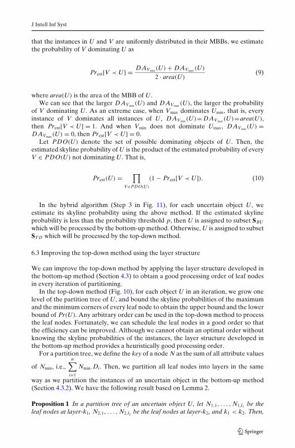
Proposition 1 In a partition tree of an uncertain object U, let N1,1, . . . , N1,l1 be theleaf nodes at layer-k1, N2,1, . . . , N2,l2 be the leaf nodes at layer-k2, and k1 < k2. Then,

J Intell Inf Syst

for any leaf node at layer-k2 N2, j2 (1 ≤ j2 ≤ l2), there exists a leaf node at layer-k1

N1, j1 (1 ≤ j1 ≤ l1) such that Pr(N1, j1 min) ≥ Pr(N2, j2 min), where N1, j1 min and N2, j2 minare the minimum corners of the MBBs of N1, j1 and N2, j2 , respectively. Moreover,

l1maxi=1

{Pr(N1,imin)} ≥ l2maxj=1

{Pr(N2, jmin)}.

According to Proposition 1, we process the leaf nodes of the partition tree of everyuncertain object U layer by layer so that the upper bound and the lower bound ofPr(U) both approach the actual value of Pr(U) quickly. Using Proposition 1, we canestimate the upper bound of Pr(Nmin) for an unprocessed leaf node N. Thus, aftera leaf node is processed, we can obtain a tighter upper bound of Pr(U) accordingto (8). Moreover, heuristically, the skyline probabilities of leaf nodes decrease as thelayer number increases. When we process the leaf nodes in the layer increasing order,the lower bound of Pr(U) also increases in a faster pace heuristically.

7 Related work

A preliminary version of this paper appeared as Pei et al. (2007b), which is thefirst paper to explore skyline analysis on uncertain data. Our study is related to theprevious work on querying uncertain data and skyline computation. In this section,we review the major existing results in these two aspects and also the work of Peiet al. (2007b) on probabilistic skyline computation.

7.1 Querying uncertain spatial data

In statistics, there are a number of tools dealing with uncertain and probabilisticdata, such as graphical models including Bayesian networks, Markov Random Fields,Influence Diagrams, etc. (Deshpande and Sarawagi 2007). Graphical models presentan option for representing the uncertainty in the data and evaluating queries overuncertain data (Dalvi and Suciu 2007; Sen et al. 2007). Particularly, they are usefulto model dependence between objects. In this paper, we assume that objects areindependent to each other. For future work, we would like to explore graphical mod-els to handle more complex relationship between objects in computing probabilisticskylines.

Modeling and querying uncertain data have also attracted considerable attentionfrom the database research community (see Aggarwal and Yu 2007; Sarma et al.2006; Dalvi and Suciu 2004, and the references therein). The work that relates closestto our problem is management and query processing of uncertain data in spatial-temporal databases (Cheng et al. 2003, 2004; Tao et al. 2005; Dai et al. 2005; Kriegelet al. 2006).

Cheng et al. (2003) proposed a broad classification of probabilistic queries overuncertain data, and developed novel techniques for evaluating probabilistic queries.Cheng et al. (2004) are the first to study probabilistic range queries. They developedtwo auxiliary index structures to support querying uncertain intervals effectively.Tao et al. (2005) investigated probabilistic range queries on multi-dimensional spacewith arbitrary probability density functions. They identified and formulated several

J Intell Inf Syst

pruning rules and proposed a new access method to optimize both I/O cost and CPUtime. Dai et al. (2005) introduced an interesting concept of ranking probabilisticspatial queries on uncertain data which selects the objects with highest probabilitiesto qualify the spatial predicates. On the uncertain data indexed by R-tree, severalefficient algorithms were developed to support ranking probabilistic range queriesand nearest neighbor queries. Kriegel et al. (2006) proposed to use probabilisticdistance functions to measure the similarity between uncertain objects. They pre-sented both the theoretical foundation and some effective pruning techniques ofprobabilistic similarity joins.

Different from the previous work on querying uncertain spatial data, our studyintroduces skyline queries and analysis to uncertain data. As shown in Sections 1and 8, skyline queries are meaningful for uncertain data and can disclose some inte-resting knowledge that cannot be identified by the existing queries on uncertain data.

7.2 Skyline computation and analysis

Computing skylines was first investigated by Kung et al. (1975) in computationalgeometry. Bentley et al. (1978) proposed an efficient algorithm with an expectedlinear runtime if the data distribution on each dimension is independent.

Borzsonyi et al. (2001) introduced the concept of skylines in the context ofdatabases and proposed a SQL syntax for skyline queries. They also developed theskyline computation techniques based on block-nested-loop and divide-and-conquerparadigms, respectively. Chomicki et al. (2003) proposed another block-nested-loopbased computation technique, SFS (sort-f ilter-skyline), to take the advantages ofpre-sorting. The SFS algorithm was further significantly improved by Godfrey et al.(2005).

The first progressive technique that can output skyline points without scanning thewhole dataset was delveloped by Tan et al. (2001). Kossmann et al. (2002) presentedanother progressive algorithm based on the nearest neighbor search technique,which adopts a divide-and-conquer paradigm on the dataset. Papadias et al. (2003)proposed a branch-and-bound algorithm (BBS) to progressively output skylinepoints on datasets indexed by an R-tree. One of the most important properties ofBBS is that it minimizes the I/O cost.

Variations of skyline computation have been explored. Pei et al. (2005, 2007a)and Yuan et al. (2005) proposed a skyline cube data structure that completely pre-computes the skylines of all possible subspaces for a given data set. Xia and Zhang(2006) addressed the incremental maintenance of skyline cubes. Tao et al. (2006)developed the SUBSKY algorithm to answer subspace skyline queries efficientlyin any subspaces. To tackle the problem of skylines in high dimensional spaces,Chan et al. (2006b) relaxed the notion of dominance to k-dominance and proposedk-dominant skylines. Dellis and Seeger (2007) proposed the reverse skyline query,which consists of objects whose dynamic skyline contains a given query point q. Thedynamic skyline of an object p corresponds to a transformed data space where pbecomes the origin and all other points are represented by their distance vectors top. Denis Mindolin (2009) investigated skylines in a case where some attributes areconsidered to be more important than the others. Lin et al. (2005), Tao and Papadias(2006), and Morse et al. (2006) answered skyline queries over data streams, where

J Intell Inf Syst

the skyline keeps updating as new data elements come and old data elements expire.Sarma et al. (2009) developed a randomized skyline algorithm for streaming. Jiangand Pei (2009) applied skyline analysis on time series data, where every data object isa time series. Balke et al. (2004) and Wu et al. (2006) computed skylines in distributedsystems. Park et al. (2009) computed skyline on multicore architectures. Huanget al. (2006) computed skyline on mobile lightweight devices such as MANETs.Sharifzadeh and Shahabi (2006) proposed spatial skyline queries, where a dimensionof a data point is the distance to some query point. Chan et al. (2005) and Sacharidiset al. (2009) considered skyline computation in partially ordered domains. Chenand Lian (2008) considered skyline queries in metric spaces. Zhang et al. (2009b)worked on skyline maintenance to handle frequent updates of the data set. Zhanget al. (2009c) estimated the skyline cardinality based on density estimation. Wonget al. (2007) and Jiang et al. (2008) used skylines to mine user preferences and makerecommendations.

All of the studies on skyline computation and analysis reviewed above focus oncertain data. Our study extends the skyline computation and analysis to uncertaindata. As shown in the previous section, extending skyline queries to uncertain datais far from straightforward. It involves both the development of skyline models andthe design of novel algorithms for efficient computation.

7.3 Probabilistic skyline computation on uncertain data

After our preliminary work (Pei et al. 2007b) introduced the concept of probabilisticskyline on uncertain data, there are some following studies adopting our probabilisticskyline model (Section 2).

Lian and Chen (2008) studied the bichromatic probabilistic reverse skyline(BPRS) queries over uncertain data. A BPRS query takes two data sets A, B anda query object q as the input, and outputs those objects o ∈ A such that the dynamicskyline of o in the data set B contains q. The dynamic skyline of an object pcorresponds to a transformed data space where p becomes the origin and all otherpoints are represented by their distance vectors to p. The main techniques to answera BPRS query also follow our bounding-pruning-refining framework.

Atallah and Qi (2009) proposed to compute the skyline probability of all instancesof all objects without setting a threshold. They developed algorithms based on aspace partitioning technique. The worst-case time complexity is sub-quadratic to thenumber of objects, however, exponential to the dimensionality. So, their algorithmsmainly focus on the 2-dimensional case, and it is not practical for higher dimensionalcases.

Böhm et al. (2009) studied the continuous case of the probabilistic skyline querywhere every object is modeled as a mixture Gaussian distribution. Their techniquescannot be applied directly to the discrete case.

Zhang et al. (2009a) extended the probabilistic skyline operator to data streamsusing a sliding window model. Their techniques are also under the bounding-pruning-refining framework with an index structure to efficiently handle updates.

The above studies investigated the variations of our p-skyline query in differentenvironments under the probabilistic skyline model. The techniques developedwithin either follow the bounding-pruning-refining framework or cannot be applieddirectly to answer p-skyline queries.

J Intell Inf Syst

8 Empirical study

In this section, we report an extensive empirical study to examine the effectivenessand the efficiency of probabilistic skyline analysis on uncertain data. All the experi-ments were conducted on a PC with Intel P4 3.0 GHz CPU and 2 GB main memoryrunning the Debian Linux operating system. All algorithms were implemented inC++.

8.1 Effectiveness of probabilistic skylines

To verify the effectiveness of probabilistic skylines on uncertain data, we use a realdata set of the NBA game-by-game technical statistics from 1991 to 2005 downloadedfrom www.NBA.com. The NBA data set contains 339,721 records about 1,313players. We treat each player as an uncertain object and the records of the player asthe instances of the object. Three attributes are selected in our analysis: number ofpoints, number of assists, and number of rebounds. The larger those attribute values,the better.

Table 2 shows the 0.1-skyline players in the skyline probability descending order.We also conducted the traditional skyline analysis. We calculated the average statis-tics for each player in each attribute. That is, each player has only one record in theaggregate data set. We computed the skyline on the aggregate data set, which is calledthe aggregate skyline for short hereafter. All skyline players in the aggregate skylineare annotated by a “*” sign in Table 2. We obtain several interesting observations.

Table 2 0.1-skyline players in skyline probability descending order

Name Skyline Name Skylineprobability probability

LeBron James* 0.350699 Magic Johnson* 0.151813Dennis Rodman* 0.327592 Chris Paul* 0.149264Shaquille O’Neal* 0.323401 Gilbert Arenas 0.142883Charles Barkley* 0.309311 Clyde Drexler 0.138993Kevin Garnett* 0.302531 Patrick Ewing 0.13577Jason Kidd* 0.293569 Rod Strickland 0.135735Allen Iverson* 0.269871 Brad Daugherty 0.133572Michael Jordan* 0.250633 Steve Francis 0.131061Tim Duncan* 0.241252 Dirk Nowitzki 0.130301Karl Malone* 0.239737 Paul Pierce 0.127079Chris Webber* 0.22153 Gary Payton* 0.126328Kevin Johnson* 0.208991 Baron Davis 0.125298Hakeem Olajuwon 0.203641 Vince Carter 0.122946Kobe Bryant 0.200272 Antoine Walker 0.121745Dwyane Wade 0.199065 Steve Nash 0.115874Tracy Mcgrady 0.198185 Andre Miller 0.11275Grant Hill* 0.191164 Isiah Thomas 0.11076John Stockton* 0.183591 Elton Brand 0.10966David Robinson 0.177437 Scottie Pippen 0.108941Stephon Marbury* 0.16683 Dominique Wilkins 0.104323Tim Hardaway* 0.166206 Lamar Odom* 0.101803

J Intell Inf Syst

First, probabilistic skylines can capture the knowledge obtained from traditionalskyline analysis. The top-12 players with the largest skyline probabilities are also inthe aggregate skyline. All of them are great players. Those players not only have goodaverage performance so that they are in the aggregate skyline, but also performedoutstandingly in some games so that they have a high skyline probability.

Second, traditional skylines can be biased by outliers. Some players that are not inthe aggregate skyline may still have a high skyline probability. There are 22 playerswho are not in the aggregate skyline, but have a higher skyline probability thanOdom who is a skyline player in the aggregate data set. Olajuwon is an example.Figure 13 plots the number of points and the number of rebounds of the game recordsof Olajuwon and Odom at a sample rate of 5% (so that the figure is readable). Weobserve that Olajuwon has some bad games (e.g, zero point and three rebounds)which hinder his average statistics. On the other hand, Odom has a few good games(e.g, more than 25 points and 12 rebounds) which help his average statistics. Butoverall, Olajuwon could be a better player since he has many more great games (e.g.,40 points and 19 rebounds).

In more details, Olajuwon is dominated by four other players in the aggregatedata set: O’Neal, Barkley, Duncan, and Webber. In Fig. 14, we plot their gamerecords. Olajuwon has some records (e.g., 40 points and 19 rebounds) dominatingmost records of other players. On the other hand, he also has some records (e.g.,zero point and three rebounds) that are dominated by many records of other players.Comparing to the four players dominating him, Olajuwon’s performance has asparser distribution.

Comparing to the aggregate skyline, the probabilistic skyline finds not only playersconsistently performing well, but also outstanding players with relatively inconsistentperformance possibly due to aging or injuries.

Third, a player A may have a higher skyline probability than a player B whodominates A in the aggregate data set. As an example, Ewing has a higher skylineprobability than Brand, though Ewing is dominated by Brand in the aggregate dataset. We plot a sample with ratio 5% of both players in Fig. 15. Their aggregate valuesare also shown in the figure. The performance of Ewing is more diverse than that

0

5

10

15

20

25

0 5 10 15 20 25 30 35 40 45

rebo

unds

points

OlajuwonOdom

Fig. 13 Comparing Olajuwon’s and Odom’s records

J Intell Inf Syst

0

5

10

15

20

25

0 5 10 15 20 25 30 35 40 45

rebo

unds

points

OlajuwonO’Neal

BarkleyDuncanWebber

Fig. 14 Olajuwon’s and some other players’ records

of Brand. Ewing played very well in a few games, which explains why Ewing has ahigher skyline probability.

In summary, probabilistic skylines disclose more knowledge about uncertain databy considering the instance distributions of objects which cannot be captured bytraditional skyline analysis, and provide a more comprehensive view on advantagesof uncertain objects than skylines using only the aggregate of such objects. Inter-estingly, we can rank uncertain objects using skyline probabilities, while the skylineon aggregate of uncertain data cannot reflect the differences on the opportunities ofuncertain objects not to be dominated by other objects. This is another significantadvantage of probabilistic skyline analysis.

8.2 Performance evaluation

To verify the efficiency and the scalability of our algorithms, we use the NBA realdata set as well as synthetic data sets in anti-correlated, independent, and correlated

0

5

10

15

20

25

0 5 10 15 20 25 30 35 40

rebo

unds

points

EwingEwing-Agg

BrandBrand-Agg

Fig. 15 Ewing’s and Brand’s records

J Intell Inf Syst

distributions. For the synthetic data sets, the domain of each dimension is [0, 1]. Thedimensionality d by default is 4. The cardinality (i.e., number of uncertain objects)m by default is 10,000. We first generated the centers of all uncertain objects usingthe benchmark data generator described in Borzsonyi et al. (2001). Then, for eachuncertain object, we use the center to generate a hyper-rectangle region where theinstances of the object appear. The edge size of the hyper-rectangle region followsa normal distribution in range [0, 0.2] with expectation 0.1 and standard deviation0.025. The instances of the object distributed uniformly in the region. The number ofinstances of an uncertain object follows uniform distribution in range [1, l], where l is400 by default. Thus, in expectation, each object has l

2 instances, and the total numberof instances in a data set is ml

2 (2,000,000 by default). The probability threshold p is0.3 unless otherwise specified. Table 3 summarizes the experiment settings.

8.2.1 Probabilistic skyline size

Figure 16 shows the size of probabilistic skylines (i.e., the number of objects ina probabilistic skyline) with respect to three important factors: the probabilitythreshold, the dimensionality and the cardinality. Generally, anti-correlated data setshave the largest skyline size. Correlated data sets have the smallest skyline size. Thisis similar to the situations of skylines on certain objects. As shown in Fig. 16a, thehigher the probability threshold, the smaller the skyline size. This is because a p-skyline contains a p′-skyline if p < p′. Figure 16b shows the results on the NBAdata set, which is in a consistent trend. Figure 16c and d show that the skyline sizeincreases with higher dimensionality and larger cardinality, which is also similar tothe situations of skylines on certain data sets. As the dimensionality increases, thedata set becomes sparser. An object has a better opportunity not to be dominated inall dimensions. As the cardinality increases, more objects may have chances not tobe dominated.

8.2.2 Ef f iciency and scalability

Figure 17 shows the overall performance of the bottom-up algorithm (BU), the top-down algorithm (TD), the hybrid algorithm (HY), and an exhaustive algorithm (EX)for benchmarking purpose. To compute the p-skyline on a data set, without anypruning techniques, EX has to compute the skyline probability for each uncertainobject. The numbers on the bars give the exact runtime of the algorithms on the datasets.

BU, TD, and HY are much faster than EX. The results clearly indicate thatthe pruning techniques in BU and TD significantly save the cost of computing theexact skyline probabilities of many instances and objects. HY is the fastest on anti-correlated and independent data sets while it is a little slower than BU on the NBAdata set.

Table 3 The summary ofexperiment settings

Notation Definition (default values)

m Cardinality of the data set (10,000)d Dimensionality of the data set (4)l Maximum number of instances per object (400)p Probability threshold (0.3)

J Intell Inf Syst

0

400

800

1200

1600

2000

2400

0.1 0.3 0.5 0.7 0.9

size

of p

-sky

line

antiindecorr

(a) Effect of p

0

20

40

60

80

100

0.05 0.1 0.15 0.2 0.25 0.3 0.35

size

of p

-sky

line

NBA

(b) Effect of p

2k

4k

6k

8k

10k

2d 4d 6d 8d 10d

size

of p

-sky

line

antiindecorr

(c) Effect of d

0

300

600

900

1200

2k 4k 6k 8k 10k

size

of p

-sky

line

antiindecorr

(d) Effect of m

Fig. 16 The size of p-skyline with respect to probability threshold p, dimensionality d, andcardinality m

Computing skylines on anti-correlated data sets is much more challenging thanthe other cases as reflected the runtime in Fig. 17. In the rest of this section, we focuson analyzing in detail the performance of our algorithms on anti-correlated data sets.

Figure 18 compares BU, TD, and HY with respect to probability threshold,dimensionality, and cardinality. All algorithms follow similar trends. The hybrid

Fig. 17 Overall performance

100

101

102

103

104

NBA anti inde corr

time(

s)

3870 4037

1434

9485170

90

7

110182

120

6

90 11368

7

EX BU TD HY

J Intell Inf Syst

0

50

100

150

200

250

0.1 0.3 0.5 0.7 0.9

time

(s)

BUTDHY

(a) Effect of p

0

50

100

150

200

250

300

2d 4d 6d 8d 10d

time

(s)

BUTDHY

(b) Effect of d

0

100

200

300

400

500

600

2k 4k 6k 8k 10k 15k 20k

time

(s)

BUTDHY

(c) Effect of m

Fig. 18 Scalability with respect to probability threshold

algorithm outperforms BU and TD and reduces the worst case runtime by 50% (e.g.,case 6d in Fig. 18b and case 20k in Fig. 18c).

Figure 18a shows that the runtime of the three algorithms decreases as theprobability threshold p increases from 0.1 to 0.9, because when p becomes larger,there are less p-skyline objects and it is easier to prune non-skyline objects. We canalso see that BU performs better than TD when p < 0.5, while worse when p ≥ 0.5.As described in Section 6, BU needs to process at least p × 100% instances of askyline object to boost the lower bound to at least p. Thus, BU runs slower than TDwhen p is large.

In Fig. 18b, the runtime of the three algorithms increases when the dimensionalityincreases from 2 to 6, but decreases afterward. On the one hand, the cost ofdominance testing between two instances, which is the basic operation in bothalgorithms, increases as the dimensionality increases. On the other hand, the averagenumber of possible dominating objects for an uncertain object decreases since thedata set becomes sparser when the dimensionality increases. The trend of runtimereflects the compromise of the two factors.

The higher the dimensionality, the sparser the data set. The larger the cardinality,the denser the data set. Figure 18b and c indicate that TD performs better when thedata set is sparser. In sparse data sets, the subset instances of uncertain objects mayhave a smaller chance to overlap, and a better chance to be pruned by some subsetinstances of other objects. Besides, objects in sparse data sets are likely to have largeskyline probabilities, since for each object, there are less possible dominating objects

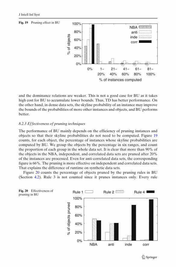
J Intell Inf Syst

Fig. 19 Pruning effect in BU

0%

20%

40%

60%

80%

100%

0% 1~ 21~ 41~ 61~ 81~%

of o

bjec

ts

% of instances computed

20% 40% 60% 80% 100%

NBAantiindecorr

and the dominance relations are weaker. This is not a good case for BU as it takeshigh cost for BU to accumulate lower bounds. Thus, TD has better performance. Onthe other hand, in dense data sets, the skyline probability of an instance may improvethe bounds of the probabilities of more other instances and objects, and BU performsbetter.

8.2.3 Ef fectiveness of pruning techniques

The performance of BU mainly depends on the efficiency of pruning instances andobjects so that their skyline probabilities do not need to be computed. Figure 19counts, for each object, the percentage of instances whose skyline probabilities arecomputed by BU. We group the objects by the percentage in six ranges, and countthe proportion of each group in the whole data set. It is clear that more than 90% ofthe objects in the NBA, independent, and correlated data sets are pruned after 20%of the instances are processed. Even for anti-correlated data sets, the correspondingfigure is 66%. The pruning is more effective on independent and correlated data sets.That explains the difference of runtime on synthetic data sets.

Figure 20 counts the percentage of objects pruned by the pruning rules in BU(Section 4.2). Rule 3 is not counted since it prunes instances only. Every rule

Fig. 20 Effectiveness ofpruning in BU

0%

20%

40%

60%

80%

100%

NBA anti inde corr

% o

f obj

ects

pru

ned

Rule 1 Rule 2 Rule 4

J Intell Inf Syst

0

10

20

30

40

0 1 2 3 4 5 6 7 8 9 10

time

(s)

partition round

(a) NBA data set

0

20

40

60

80

0 1 2 3 4 5 6 7 8 9

time

(s)

partition round

antiindecorr

(b) Synthetic data sets

Fig. 21 Pruning effect in TD—runtime in each round

takes effect in some situations. Rule 4 is particularly effective on independent andcorrelated data sets where 84 and 97% objects are pruned, respectively. In thosedata sets, it is more likely that an object is completely dominated by another.

Figures 21 and 22 examine the effectiveness of the pruning techniques in TD.Figure 21a and b show the runtime of each round of partitioning on the NBA dataset and the synthetic data sets, respectively. On all data sets, the runtime increasesat first, since after such a round the leaf nodes not pruned are partitioned into morenodes. The runtime decreases in the later rounds. This is because the effectivenessof pruning in TD becomes stronger when the leaf nodes are smaller, such that thenumbers of remaining objects and nodes decrease significantly.

Figure 22 shows in each round the number of objects whose probabilistic skylinememberships are determined. Recall that in round 0, the top-down method prunesuncertain objects using their MBBs. On the NBA data set, rounds 2–8 prune mostof the objects, while on the synthetic data sets, most of the objects are pruned in thefirst round. Again, the pruning is more effective on independent and correlated datasets.

In summary, our two algorithms are effective and efficient in computing proba-bilistic skylines. They are also scalable on our large data sets containing millions ofinstances.

0%

10%

20%

30%

0 1 2 3 4 5 6 7 8 9 10

% o

f obj

ects

pru

ned

partition round

(a) NBA data set

0%

20%

40%

60%

80%

100%

0 1 2 3 4 5 6 7 8 9

% o

f obj

ects

pru

ned

partition round

antiindecorr

(b) Synthetic data sets

Fig. 22 Pruning effect in TD—percentage of objects pruned in each round

J Intell Inf Syst

9 Discussion and conclusions

In this paper, we extended the well-known skyline analysis to uncertain data, and de-veloped four efficacious algorithms to tackle the problem of computing probabilisticskylines on uncertain data. Using real data sets and synthetic data sets, we illustratedthe effectiveness of probabilistic skylines and the efficiency and scalability of ouralgorithms.

Although we focused on the discrete case, some of our ideas can be applied tohandle the continuous case, i.e., each uncertain object is represented by a probabilitydensity function. For example, in the top-down algorithm, for each uncertain object,we can initially partition the space into two regions such that the probability of theobject in each region is 0.5. Each region can be represented by a bounding box. Wecan estimate the skyline probabilities of the bounding boxes and recursively partitionthe bounding boxes into smaller ones until the skyline probabilities of uncertainobjects can be determined against the threshold. A detailed exploration on efficientmethods for computing probabilistic skylines on continuous data will be given byanother study.

Advanced data analysis on uncertain data is an interesting direction. In the future,we plan to exploit the probabilistic skyline analysis in real applications, and exploremore analytical tasks on uncertain data.

References

Abiteboul, S., Kanellakis, P., & Grahne, G. (1987). On the representation and querying of setsof possible worlds. In Proceedings of the 1987 ACM SIGMOD international conference onManagement of data (SIGMOD’87) (pp. 34–48). New York: ACM Press.

Aggarwal, C. C., & Yu, P. S. (2007). A survey of uncertain data algorithms and applications. IBMtechnical report (RC 24394).

Atallah, M. J., & Qi, Y. (2009). Computing all skyline probabilities for uncertain data. In Proceedingsof the twenty-eigth ACM SIGMOD-SIGACT-SIGART symposium on principles of databasesystems, PODS (pp. 279–287).

Balke, W. T., Güntzer, U., & Zheng, J. X. (2004). Efficient distributed skylining for web informationsystems. In EDBT 2004, 9th international conference on extending database technology (pp. 256–273).

Benjelloun, O., Sarma, A. D., Halevy, A., & Widom, J. (2006). Uldbs: Databases with uncertaintyand lineage. In VLDB’2006: Proceedings of the 32nd international conference on very large databases, VLDB endowment (pp. 953–964).

Bentley, J. L. (1975). Multidimensional binary search trees used for associative searching. Commu-nications of the ACM (CACM), 18(9), 509–517.

Bentley, J. L., Kung, H. T., Schkolnick, M., & Thompson, C. D. (1978). On the average number ofmaxima in a set of vectors and applications. Journal of the ACM, 25(4), 536–543.

Böhm, C., Fiedler, F., Oswald, A., Plant, C., & Wackersreuther, B. (2009). Probabilistic skylinequeries. In Proceedings of the 18th ACM conference on information and knowledge management,CIKM (pp. 651–660).

Borzsonyi, S., Kossmann, D., & Stocker, K. (2001). The skyline operator. In Proceedings of 2001international conferences on data engineering (ICDE’01). Heidelberg, Germany.

Burdick, D., Deshpande, P. M., Jayram, T. S., Ramakrishnan, R., & Vaithyanathan, S. (2005). OLAPover uncertain and imprecise data. In VLDB ’05: Proceedings of the 31st international conferenceon very large data bases, VLDB endowment (pp. 970–981).

Chan, C. Y., Eng, P. K., & Tan, K. L. (2005). Stratified computation of skylines with partially-ordereddomains. In Proceedings of the 2005 ACM SIGMOD international conference on management ofdata (SIGMOD) (pp. 203–214).

J Intell Inf Syst

Chan, C. Y., Jagadish, H. V., Tan, K. L., Tung, A. K. H., & Zhang, Z. (2006a). Finding k-dominantskylines in high dimensional space. In Proceedings of the 2006 ACM SIGMOD internationalconference on management of data (SIGMOD) (pp. 503–514).

Chan, C. Y., Jagadish, H. V., Tan, K. L., Tung, A. K. H., & Zhang, Z. (2006b). Finding k-dominantskylines in high dimensional space. In SIGMOD (pp. 503–514). New York: ACM Press.

Chan, C. Y., Jagadish, H. V., Tan, K. L., Tung, A. K. H., & Zhang, Z. (2006c). On high dimensionalskylines. In 10th international conference on extending database technology (EDBT) (pp. 478–495).

Chen, L., & Lian, X. (2008). Dynamic skyline queries in metric spaces. In EDBT (pp. 333–343).Cheng, R., Kalashnikov, D. V., & Prabhakar, S. (2003). Evaluating probabilistic queries over impre-

cise data. In Proceedings of the 2003 ACM SIGMOD international conference on management ofdata (SIGMOD’03) (pp. 551–562). New York: ACM Press.

Cheng, R., Xia, Y., Prabhakar, S., Shah, R., & Vitter, J. S. (2004). Efficient indexing methodsfor probabilistic threshold queries over uncertain data. In Proceedings of 30th internationalconference on very large data bases (VLDB) (pp. 876–887).

Chomicki, J., Godfrey, P., Gryz, J., & Liang, D. (2003). Skyline with presorting. In Proceedings of the19th international conference on data engineering (ICDE) (pp. 717–816).

Dai, X., Yiu, M. L., Mamoulis, N., Tao, Y., & Vaitis, M. (2005). Probabilistic spatial queries onexistentially uncertain data. In Proceeding of the 9th international symposium on spatial andtemporal databases (SSTD) (pp. 400–417).

Dalvi, N. N., & Suciu, D. (2004). Efficient query evaluation on probabilistic databases. In Proceedingsof 30th international conference on very large data bases (VLDB) (pp. 864–875).

Dalvi, N. N., & Suciu, D. (2007). Management of probabilistic data: Foundations and challenges. InProceedings of the twenty-sixth ACM SIGACT-SIGMOD-SIGART symposium on principles ofdatabase systems (pp. 1–12). New York: ACM Press.

Dellis, E., & Seeger, B. (2007). Efficient computation of reverse skyline queries. In Proceedings ofthe 33rd international conference on very large data bases (VLDB) (pp. 291–302).

Denis Mindolin, J. C. (2009). Discovering relative importance of skyline attributes. In Proceedingsof the 35th international conference on very large data bases (VLDB).

Deshpande, A., & Sarawagi, S. (2007). Probabilistic graphical models and their role in databases. InProceedings of the 33rd international conference on very large data bases (pp. 1435–1436).

Godfrey, P., Shipley, R., & Gryz, J. (2005). Maximal vector computation in large data sets. In VLDB.Trondheim, Norway.

Guttman, A. (1984). R-tree: A dynamic index structure for spatial searching. In Proc. 1984 ACM-SIGMOD int. conf. management of data (SIGMOD’84) (pp. 47–57). Boston, MA.

Huang, Z., Jensen, C. S., Lu, H., & Ooi, B. C. (2006). Skyline queries against mobile lightweightdevices in manets. In Proceedings of the 22nd international conference on data engineering(ICDE’06). New York: IEEE.

Imielinski, T., & Witold Lipski, J. (1984). Incomplete information in relational databases. Journal ofthe ACM, 31(4), 761–791.

Jiang, B., & Pei, J. (2009). Online interval skyline queries on time series. In Proceedings of the 25thinternational conference on data engineering (ICDE’09). Shanghai, China.

Jiang, B., Pei, J., Lin, X., Cheung, D. W., & Han, J. (2008). Mining preferences from superior andinferior examples. In KDD ’08: Proceeding of the 14th ACM SIGKDD international conferenceon knowledge discovery and data mining (pp. 390–398). New York: ACM Press.

Kossmann, D., Ramsak, F., & Rost, S. (2002). Shooting stars in the sky: An online algorithmfor skyline queries. In Proc. 2002 int. conf. on very large data bases (VLDB’02). Hong Kong,China.

Kriegel, H. P., Kunath, P., Pfeifle, M., & Renz, M. (2006). Probabilistic similarity join on uncertaindata. In Proceeding of the 11th international conference on database systems for advanced appli-cations (DASFAA) (pp. 295–309).

Kung, H. T., Luccio, F., & Preparata, F. P. (1975). On finding the maxima of a set of vectors. Journalof the ACM, 22(4), 469–476.

Lian, X., & Chen, L. (2008). Monochromatic and bichromatic reverse skyline search over uncertaindatabases. In SIGMOD conference (pp. 213–226).

Lin, X., Yuan, Y., Wang, W., & Lu, H. (2005). Stabbing the sky: Efficient skyline computation oversliding windows. In Proceedings of the 21st international conference on data engineering (ICDE)(pp. 502–513).

Morse, M. D., Patel, J. M., & Grosky, W. I. (2006). Efficient continuous skyline computation. InProceedings of the 22nd international conference on data engineering (ICDE) (p. 108).

J Intell Inf Syst

Papadias, D., Tao, Y., Fu, G., & Seeger, B. (2003). An optimal and progressive algorithm for skylinequeries. In Proceedings of the 2003 ACM SIGMOD international conference on management ofdata (SIGMOD) (pp. 467–478).

Park, S., Kim, T., Park, J., Kim, J., & Im, H. (2009). Parallel skyline computation on multicorearchitectures. In Proceedings of the 25th international conference on data engineering, ICDE(pp. 760–771).

Pei, J., Jin, W., Ester, M., & Tao, Y. (2005). Catching the best views in skyline: A semantic approach.In Proceedings of the 31st international conference on very large data bases (VLDB’05).

Pei, J., Fu, A. W. C., Lin, X., & Wang, H. (2007a). Computing compressed skyline cubes efficiently. InProceedings of the 23rd international conference on data engineering (ICDE’07). IEEE, Istanbul.

Pei, J., Jiang, B., Lin, X., & Yuan, Y. (2007b). Probabilistic skylines on uncertain data. In Proceedingsof the 33rd international conference on very large data bases (VLDB’07). Viena, Austria.

Sacharidis, D., Papadopoulos, S., & Papadias, D. (2009). Topologically sorted skylines for partiallyordered domains. In Proceedings of the 25th international conference on data engineering, ICDE(pp. 1072–1083).

Sarma, A. D., Benjelloun, O., Halevy, A. Y., & Widom, J. (2006). Working models for uncertaindata. In Proceedings of the 22nd international conference on data engineering (ICDE) (p. 7).

Sarma, A. D., Lall, A., Nanongkai, D., & Xu, J. (2009). Randomized multi-pass streaming skylinealgorithms. In Proceedings of the 35th international conference on very large data bases.

Sen, P., Deshpande, A., & Getoor, L. (2007). Representing tuple and attribute uncertainty in prob-abilistic databases. In Workshops proceedings of the 7th IEEE international conference on datamining (ICDM) (pp. 507–512). Los Alamitos: IEEE Computer Society.

Sharifzadeh, M., & Shahabi, C. (2006). The spatial skyline queries. In Proceedings of the 32ndinternational conference on very large data bases (VLDB) (pp. 751–762).

Soliman, M. A., Ilyas, I. F., & Chang, K. C. C. (2007). Top-k query processing in uncertain databases.In Proceedings of the 23rd international conference on data engineering (ICDE’07). New York:IEEE.

Tan, K. L., Eng, P. K., & Ooi, B. C. (2001). Efficient progressive skyline computation. In Proceedingsof 27th international conference on very large data bases (VLDB) (pp. 301–310).

Tao, Y., & Papadias, D. (2006). Maintaining sliding window skylines on data streams. IEEE Trans-actions on Knowledge and Data Engineering, 18(2), 377–391.

Tao, Y., Cheng, R., Xiao, X., Ngai, W. K., Kao, B., & Prabhakar, S. (2005). Indexing multi-dimensional uncertain data with arbitrary probability density functions. In Proceedings of 31stinternational conference on very large data bases (VLDB) (pp. 922–933).

Tao, Y., Xiao, X., & Pei, J. (2006). Subsky: Efficient computation of skylines in subspaces. InProceedings of the 22nd international conference on data engineering (ICDE’06). New York:IEEE.

Wong, R. C. W., Pei, J., Fu, A. W. C., & Wang, K. (2007). Mining favorable facets. In KDD ’07:Proceedings of the 13th ACM SIGKDD international conference on knowledge discovery anddata mining (pp. 804–813). New York: ACM.

Wu, P., Zhang, C., Feng, Y., Zhao, B. Y., Agrawal, D., & Abbadi, A. E. (2006). Parallelizing skylinequeries for scalable distribution. In Proceedings of the 10th international conference on extendingdatabase technology (EDBT’06). Munich: Springer.

Xia, T., & Zhang, D. (2006). Refreshing the sky: The compressed skycube with efficient supportfor frequent updates. In Proceedings of the 2006 ACM SIGMOD international conference onmanagement of data (SIGMOD’06) (pp. 491–502). New York: ACM Press.

Yuan, Y., Lin, X., Liu, Q., Wang, W., Yu, J. X., & Zhang, Q. (2005). Efficient computation of theskyline cube. In Proceedings of the 31st international conference on very large data bases (VLDB)(pp. 241–252).

Zhang, W., Lin, X., Zhang, Y., Wang, W., & Yu, J. X. (2009a). Probabilistic skyline operator oversliding windows. In Proceedings of the 25th international conference on data engineering, ICDE(pp. 1060–1071).

Zhang, Z., Cheng, R., Papadias, D., & Tung, A. K. H. (2009b). Minimizing the communicationcost for continuous skyline maintenance. In Proceedings of the ACM SIGMOD internationalconference on management of data. Providence, RI, USA.

Zhang, Z., Yang, Y., Cai, R., Papadias, D., & Tung, A. K. H. (2009c). Kernel-based skyline cardinal-ity estimation. In Proceedings of the ACM SIGMOD international conference on management ofdata.