PROBABILISTIC MODELS FOR REGION-BASED SCENE A …
203
PROBABILISTIC MODELS FOR REGION-BASED SCENE UNDERSTANDING A DISSERTATION SUBMITTED TO THE DEPARTMENT OF ELECTRICAL ENGINEERING AND THE COMMITTEE ON GRADUATE STUDIES OF STANFORD UNIVERSITY IN PARTIAL FULFILLMENT OF THE REQUIREMENTS FOR THE DEGREE OF DOCTOR OF PHILOSOPHY Stephen Gould June 2010
Transcript of PROBABILISTIC MODELS FOR REGION-BASED SCENE A …

PROBABILISTIC MODELS FOR REGION-BASED SCENE
UNDERSTANDING
A DISSERTATION
SUBMITTED TO THE DEPARTMENT OF ELECTRICAL
ENGINEERING
AND THE COMMITTEE ON GRADUATE STUDIES
OF STANFORD UNIVERSITY
IN PARTIAL FULFILLMENT OF THE REQUIREMENTS
FOR THE DEGREE OF
DOCTOR OF PHILOSOPHY
Stephen Gould
June 2010

c© Copyright by Stephen Gould 2010
All Rights Reserved
ii

I certify that I have read this dissertation and that, in my opinion, it
is fully adequate in scope and quality as a dissertation for the degree
of Doctor of Philosophy.
(Daphne Koller) Principal Adviser
I certify that I have read this dissertation and that, in my opinion, it
is fully adequate in scope and quality as a dissertation for the degree
of Doctor of Philosophy.
(Andrew Y. Ng)
I certify that I have read this dissertation and that, in my opinion, it
is fully adequate in scope and quality as a dissertation for the degree
of Doctor of Philosophy.
(Stephen P. Boyd)
Approved for the University Committee on Graduate Studies.
iii

iv

Abstract
One of the long-term goals of computer vision is to be able to understand the world
through visual images. This daunting task involves reasoning simultaneously about
objects, regions and the 3D geometric relationship between them. Traditionally, com-
puter vision research has tackled this reasoning in isolation: independent detectors
for finding objects, image segmentation algorithms for defining regions, and special-
ized monocular depth perception methods for reconstructing geometry. This method
of isolated reasoning, however, can lead to inconsistent interpretations of the scene.
For example, one algorithm may reason that a particular bounding box contains an
object while another algorithm reasons that those same pixels be labeled something
completely different, e.g., sky or grass.
In this thesis we present a unified probabilistic model that avoids these inconsis-
tencies. We develop our model in stages: First, we introduce a region-based represen-
tation of the scene in which pixels are grouped together into consistent regions, and
each region is annotated with a semantic and geometric class label. Our semantic
labels consist of a number of background classes (e.g., sky, grass, road) and a single
generic foreground object class. Importantly, all pixels are uniquely explained by this
representation. Our model defines an energy function, or factored scoring function,
over this representation which allows us to evaluate the quality of any given decom-
position of the scene. We present an efficient move-making algorithm that allows us
to perform approximate maximum a posteriori (MAP) inference in this model given
a novel image.
Next, we extend our model by introducing the concept of objects. Here, we build
v

on the region-based representation by allowing foreground regions to be grouped to-
gether into coherent objects. For example, grouping separate head, torso and legs re-
gions into a single person object. We add corresponding terms to our energy function
that allow us to recognize these objects and model contextual relationships between
objects and adjacent regions. For example, we would expect to find cars on road and
boats on water. We also extend our inference algorithm to allow for larger top-down
moves to be evaluated.
Last, we show how our region-based approach can be used to interpret the 3D
structure of the scene and estimate depth, resulting in a complete understanding of
regions, objects, and geometry.
vi

For Lesley.
vii

viii

Acknowledgments
I feel truly privileged to have had the opportunity to work with Daphne Koller, who
always puts the needs of her students above anything else. Thank you, Daphne, for
your encouragement and support, but most importantly the inspiration that you have
provided me over the past five years. Your technical brilliance, research insight, and
professional standards make you an ideal role model and mentor.
I am also profoundly grateful to Andrew Ng, with whom I worked during the first
few years of my Ph.D., and who has continued to offer guidance and show interest in
my work. Thank you, Andrew, for your generous advice over the years.
I would like to thank Stephen Boyd, who was my Masters academic advisor (way
back in 1997) and has been an inspiration to me ever since. His casual style com-
bined with technical clarity have been a great example to me. Thank you to Kalanit
Grill-Spector for chairing my defense at short notice and for providing a different
perspective on my research.
I am indebted to Gal Elidan, Geremy Heitz, and Ben Packer who helped induct
me into the DAGS research group and, almost as important, the morning coffee
ritual. I will always cherish the memories of our excursions to Peet’s Coffee. Thanks
also to Pawan Kumar for his guidance during the later stages of my thesis (and for
introducing a bit of British tea into our morning coffee).
I also owe a great deal to the many friends and colleagues that I have met at
Stanford—Pieter Abbeel, Fernando Amat, Alexis Battle, Vasco Chatalbashev, Gal
Chechik, Adam Coates, David Cohen, James Diebel, Yoni Donner, John Duchi, Varun
Ganapathi, Tianshi Gao, Vladimir Jojic, Adrian Kaehler, Joni Laserson, Quoc Le,
Honglak Lee, Su-in Lee, Beyang Liu, Farshid Moussavi, Suchi Saria, Christina Pop,
ix

Morgan Quigley, Jim Rodgers, Olga Russakovsky, Ashutosh Saxena, David Vickrey,
Haidong Wang, Huayan Wang—and to the numerous undergraduate and masters
students with whom I’ve worked—Ravi Parikh, Rick Fulton, Evan Rosen, Ben Sapp,
Marius Meissner, Ian Goodfellow, Sid Batra, Paul Baumstarck, and many others.
Thank you all for the ideas, advice, and contributions you have made to my research.
I am also indebted to the many academics and visiting researchers with whom I’ve
interacted over the past several years. In particular, I give warm thanks to Jana
Kosecka, Richard Zemel, Gary Bradski and Fei-Fei Li for providing external view-
points.
Most importantly, I would like to thank my wonderful family. First, to my dad,
Arnold, my sister, Hayley, and all my family back in Australia, I thank you for your
continued support and encouragement from abroad. Last, to my wife Naomi: the
decision to move from our comfortable professional lives in Australia to the life of a
“graduate student couple” at Stanford has been an adventure. Thank you, Naomi,
for plunging into this adventure with me, for your continued love and support, and
for keeping our lives normal. While all I had to do was write some scientific papers
and a couple of lines of code, you had the formidable task of raising a family—a task
at which you have excelled. To my two gorgeous daughters, Ariella and Bronte, I
thank you for your smiles, your laughs, your 4am wake-ups, your tantrums, and your
questions—as a scientist there is no better question to hear than “Why, daddy?”.
When you get older, I hope you appreciate how much all of these mean to me.
x

Contents
Abstract v
Acknowledgments ix
1 Introduction 1
1.1 Contributions . . . . . . . . . . . . . . . . . . . . . . . . . . . . . . . 5
1.2 Thesis Outline . . . . . . . . . . . . . . . . . . . . . . . . . . . . . . . 7
1.3 Related Work . . . . . . . . . . . . . . . . . . . . . . . . . . . . . . . 9
1.4 Previously Published Work . . . . . . . . . . . . . . . . . . . . . . . . 17
2 Background 19
2.1 Machine Learning and Graphical Models . . . . . . . . . . . . . . . . 19
2.1.1 Classification and Regression . . . . . . . . . . . . . . . . . . . 20
2.1.2 Probabilistic Graphical Models . . . . . . . . . . . . . . . . . 25
2.2 Computer Vision . . . . . . . . . . . . . . . . . . . . . . . . . . . . . 32
2.2.1 Image Formation . . . . . . . . . . . . . . . . . . . . . . . . . 32
2.2.2 Low Level Image Features . . . . . . . . . . . . . . . . . . . . 35
2.2.3 Sliding-Window Object Detection . . . . . . . . . . . . . . . . 38
2.2.4 Image Segmentation . . . . . . . . . . . . . . . . . . . . . . . 46
2.3 Chapter Summary . . . . . . . . . . . . . . . . . . . . . . . . . . . . 51
3 Image Datasets and Dataset Construction 53
3.1 Standard Image Datasets . . . . . . . . . . . . . . . . . . . . . . . . . 54
3.2 Stanford Background Dataset . . . . . . . . . . . . . . . . . . . . . . 58
xi

3.2.1 Amazon Mechanical Turk . . . . . . . . . . . . . . . . . . . . 58
3.3 Chapter Summary . . . . . . . . . . . . . . . . . . . . . . . . . . . . 61
4 Scene Decomposition 67
4.1 Scene Decomposition Model . . . . . . . . . . . . . . . . . . . . . . . 70
4.1.1 Predicting Horizon Location . . . . . . . . . . . . . . . . . . . 71
4.1.2 Characterizing Individual Region Appearance . . . . . . . . . 72
4.1.3 Individual Region Potentials . . . . . . . . . . . . . . . . . . . 74
4.1.4 Inter-Region Potentials . . . . . . . . . . . . . . . . . . . . . . 76
4.2 Inference and Learning . . . . . . . . . . . . . . . . . . . . . . . . . . 79
4.2.1 Inference Algorithm . . . . . . . . . . . . . . . . . . . . . . . . 79
4.2.2 Learning Algorithm . . . . . . . . . . . . . . . . . . . . . . . . 81
4.3 Experiments . . . . . . . . . . . . . . . . . . . . . . . . . . . . . . . . 83
4.3.1 Baselines . . . . . . . . . . . . . . . . . . . . . . . . . . . . . . 84
4.3.2 Region-based Approach . . . . . . . . . . . . . . . . . . . . . 84
4.3.3 Comparison with Other Methods . . . . . . . . . . . . . . . . 86
4.4 Chapter Summary . . . . . . . . . . . . . . . . . . . . . . . . . . . . 87
5 Object Detection and Outlining 93
5.1 Region-based Model for Object Detection . . . . . . . . . . . . . . . . 96
5.1.1 Energy Function . . . . . . . . . . . . . . . . . . . . . . . . . 97
5.1.2 Object Features . . . . . . . . . . . . . . . . . . . . . . . . . . 102
5.2 Inference and Learning . . . . . . . . . . . . . . . . . . . . . . . . . . 107
5.2.1 Inference . . . . . . . . . . . . . . . . . . . . . . . . . . . . . . 107
5.2.2 Proposal Moves . . . . . . . . . . . . . . . . . . . . . . . . . . 108
5.2.3 Learning . . . . . . . . . . . . . . . . . . . . . . . . . . . . . . 112
5.3 Experiments . . . . . . . . . . . . . . . . . . . . . . . . . . . . . . . . 113
5.3.1 Street Scenes Dataset . . . . . . . . . . . . . . . . . . . . . . . 113
5.3.2 Cascaded Classification Models Dataset . . . . . . . . . . . . . 116
5.4 Chapter Summary . . . . . . . . . . . . . . . . . . . . . . . . . . . . 120
xii

6 Scene Reconstruction 125
6.1 Geometric Reconstruction . . . . . . . . . . . . . . . . . . . . . . . . 128
6.2 Depth Estimation . . . . . . . . . . . . . . . . . . . . . . . . . . . . . 131
6.2.1 Encoding Geometric Constraints . . . . . . . . . . . . . . . . 133
6.2.2 Features and Pointwise Depth Estimation . . . . . . . . . . . 134
6.2.3 MRF Model for Depth Reconstruction . . . . . . . . . . . . . 137
6.3 Experiments . . . . . . . . . . . . . . . . . . . . . . . . . . . . . . . . 139
6.4 Chapter Summary . . . . . . . . . . . . . . . . . . . . . . . . . . . . 143
7 Conclusions and Future Directions 149
7.1 Summary . . . . . . . . . . . . . . . . . . . . . . . . . . . . . . . . . 149
7.2 Open Problems and Future Directions . . . . . . . . . . . . . . . . . 151
7.2.1 Learning from Multiple Sources . . . . . . . . . . . . . . . . . 151
7.2.2 Structure and Occlusion . . . . . . . . . . . . . . . . . . . . . 152
7.2.3 Expanding the Object Classes . . . . . . . . . . . . . . . . . . 153
7.2.4 Hierarchical Decomposition . . . . . . . . . . . . . . . . . . . 154
7.2.5 Activity Recognition . . . . . . . . . . . . . . . . . . . . . . . 155
7.3 Conclusion . . . . . . . . . . . . . . . . . . . . . . . . . . . . . . . . . 155
A Implementation Details 157
A.1 Region Appearance Features . . . . . . . . . . . . . . . . . . . . . . . 158
A.2 Checking for Connected Components . . . . . . . . . . . . . . . . . . 161
Bibliography 181
xiii

xiv

List of Tables
4.1 Local pixel appearance features, αp. . . . . . . . . . . . . . . . . . . . 73
4.2 Summary of the features φr(Ar,Pr) used to describe regions. . . . . . 75
4.3 Summary of the features φrs(Ar,Pr, As,Ps) used to describe the pair-
wise relationship between two adjacent regions. . . . . . . . . . . . . 78
4.4 Multi-class image segmentation and surface orientation (geometry) ac-
curacy on the Stanford Background Dataset. . . . . . . . . . . . . . . 84
4.5 Comparison with state-of-the-art 21-class MSRC results against our
restricted model. . . . . . . . . . . . . . . . . . . . . . . . . . . . . . 87
4.6 Comparison with state-of-the-art Geometric Context results against
our restricted model. . . . . . . . . . . . . . . . . . . . . . . . . . . . 87
5.1 Summary of the features φor(Po,Pr) used to describe the contextual
pairwise relationship between an object o and adjacent region r. . . . 102
5.2 Summary of the features φo(Po, vhz, I) used to describe an object in
our model. . . . . . . . . . . . . . . . . . . . . . . . . . . . . . . . . . 106
5.3 Object detections results for the Street Scenes dataset. . . . . . . . . 114
5.4 Precision and recall for each object category calculated on the MAP
assignment. . . . . . . . . . . . . . . . . . . . . . . . . . . . . . . . . 118
5.5 Object detections results for the CCM dataset. . . . . . . . . . . . . . 119
6.1 Quantitative results comparing variants of our “semantic-aware” ap-
proach with strong baselines and other state-of-the-art methods. . . . 140
6.2 Quantitative results by predicted semantic class (log10 error). . . . . . 142
6.3 Quantitative results by predicted semantic class (relative error). . . . 142
xv

xvi
List of Figures
1.1 Inconsistent results in attempting to understanding a scene using sep-
arate computer vision tasks. . . . . . . . . . . . . . . . . . . . . . . . 3
1.2 Illustration of the aim of this thesis to understanding outdoor scenes
in terms of regions, objects and geometry. . . . . . . . . . . . . . . . 4
1.3 Hierarchical model of a scene. . . . . . . . . . . . . . . . . . . . . . . 6
2.1 Example of a simple pairwise CRF. . . . . . . . . . . . . . . . . . . . 27
2.2 The geometry of image formation. . . . . . . . . . . . . . . . . . . . . 33
2.3 Convolution of an image with a filter. . . . . . . . . . . . . . . . . . . 35
2.4 The SIFT feature descriptor. . . . . . . . . . . . . . . . . . . . . . . . 37
2.5 Illustration of the 17-dimensional “texton” filters used in multi-class
image segmentation. . . . . . . . . . . . . . . . . . . . . . . . . . . . 38
2.6 Application of 17-dimensional “texton” filters to an image. . . . . . . 39
2.7 Sliding-window object detection. . . . . . . . . . . . . . . . . . . . . . 40
2.8 Feature construction for HOG-based object detector. . . . . . . . . . 41
2.9 Feature construction for patch-based object detector. . . . . . . . . . 42
2.10 Measuring object detection performance. . . . . . . . . . . . . . . . . 44
2.11 Comparison of different unsupervised image segmentation algorithms. 47
2.12 Illustration of a conditional Markov random field for multi-class image
labeling. . . . . . . . . . . . . . . . . . . . . . . . . . . . . . . . . . . 51
3.1 Screenshot of an Amazon Mechanical Turk HIT for labeling regions in
an image. . . . . . . . . . . . . . . . . . . . . . . . . . . . . . . . . . 62
3.2 Typical label quality obtained from AMT jobs. . . . . . . . . . . . . . 63
xvii
3.3 Comparison of the label quality obtained from our AMT jobs versus
the 21-class MSRC dataset. . . . . . . . . . . . . . . . . . . . . . . . 64
3.4 Two examples of poorly labeled images obtained from a semantic la-
beling job on Amazon Mechanical Turk (AMT). . . . . . . . . . . . . 65
4.1 Example of a typical urban scene. . . . . . . . . . . . . . . . . . . . . 68
4.2 Example over-segmentation dictionary, Ω, for a given image. . . . . . 80
4.3 Examples of typical scene decompositions produced by our method. . 86
4.4 Representative results when our scene decomposition model does well. 90
4.5 Examples of where our scene decomposition algorithm makes mistakes. 91
5.1 Contextual information is critical for recognizing small objects. . . . . 96
5.2 An illustration of random variables defined by our joint object detec-
tion and scene decomposition model. . . . . . . . . . . . . . . . . . . 98
5.3 Illustration of soft masks for proposed object regions. . . . . . . . . . 105
5.4 Illustration of a preprocessed top-down object proposal move. . . . . 111
5.5 Illustration of eroding a top-down bounding box move. . . . . . . . . 112
5.6 Object detection precision-recall curves for patch-based and HOG-
based detectors on the Street Scenes dataset. . . . . . . . . . . . . . . 115
5.7 Example output from our joint scene decomposition and object detec-
tion algorithm. . . . . . . . . . . . . . . . . . . . . . . . . . . . . . . 116
5.8 Qualitative object detection results for the Street Scenes dataset. . . 117
5.9 Object detection precision-recall curves for patch-based and HOG-
based detectors on the CCM dataset. . . . . . . . . . . . . . . . . . . 120
5.10 Qualitative object detection results for the CCM dataset. . . . . . . . 123
5.11 Failure modes of our scene understanding algorithm. . . . . . . . . . 124
6.1 Example output from our semantically-aware depth estimation model. 126
6.2 Schematic illustrating geometric reconstruction of a simple scene. . . 129
6.3 Novel views of a scene with foreground objects generated by geometric
reconstruction. . . . . . . . . . . . . . . . . . . . . . . . . . . . . . . 131
6.4 Illustration of semantically derived geometric constraints. . . . . . . . 133
xviii

6.5 Smoothed per-pixel log-depth prior for each semantic class. . . . . . . 135
6.6 Graph showing the effect of using the Huber penalty for constraining
depth range. . . . . . . . . . . . . . . . . . . . . . . . . . . . . . . . . 138
6.7 Plot of log10 error metric versus relative error metric comparing algo-
rithms from Table 6.1. . . . . . . . . . . . . . . . . . . . . . . . . . . 141
6.8 Quantitative depth estimation results on the Make3d dataset. . . . . 146
6.9 Novel 3D views of different scenes generated from our semantically-
aware depth reconstruction model. . . . . . . . . . . . . . . . . . . . 147
A.1 Feature matrices for storing pixel feature vectors. . . . . . . . . . . . 158
A.2 Integral images and row integrals. . . . . . . . . . . . . . . . . . . . . 160
A.3 4-connected and 8-connected neighborhoods. . . . . . . . . . . . . . . 162
xix

xx

List of Algorithms
2.1 Discrete AdaBoost . . . . . . . . . . . . . . . . . . . . . . . . . . . . . 24
2.2 Iterated Conditional Modes (ICM) . . . . . . . . . . . . . . . . . . . . 28
2.3 Factor Addition . . . . . . . . . . . . . . . . . . . . . . . . . . . . . . 30
2.4 Min-Sum Message Passing . . . . . . . . . . . . . . . . . . . . . . . . . 31
2.5 Mean-shift Segmentation . . . . . . . . . . . . . . . . . . . . . . . . . 48
4.1 Scene Decomposition Inference. . . . . . . . . . . . . . . . . . . . . . . 81
5.1 Scene Decomposition with Objects Inference. . . . . . . . . . . . . . . 109
A.1 Compute Region Features. . . . . . . . . . . . . . . . . . . . . . . . . . 164
A.2 Find Connected Components. . . . . . . . . . . . . . . . . . . . . . . . 165
xxi

xxii

Chapter 1
Introduction
One of the long-term goals of Artificial Intelligence (AI) is to develop autonomous
agents (i.e., machines) that can reason about their environments from visual in-
puts [Russell and Norvig, 2002]. This ambitious goal manifests itself in many appli-
cations including robot perception for navigation, inventory taking and manipulation
(e.g., [Newman et al., 2006, Klingbeil et al., 2010, Quigley et al., 2009, Saxena et al.,
2007]); surveillance for physical security and environmental monitoring (e.g., [Thirde
et al., 2006]); interpretation of medical images for diagnosis and computer-assisted
surgery (e.g., [Mirota et al., 2009]); and understanding of Internet images for search
and knowledge acquisition (e.g., [Lew et al., 2006, Li et al., 2007]). Each of these
diverse applications requires complex reasoning about the interactions between the
real-world entities that give rise to the visual inputs that we, or our machines, per-
ceive. For example, to understand a photograph of a visual scene we need to reason
about objects (some of which may be partially occluded), background regions, sur-
face color and reflectance properties, 3D structure, image scale, lighting, the complex
interactions between all of them.
To further appreciate the challenges of automatic scene understanding, consider
that a machine is presented with a description of the scene as a rectangular array
of numbers. (We will discuss image formation in more detail in Section 2.2.1.) It is
from this very plain representation that we need to bring the scene back to life by
discovering the underlying structure and objects within it.
1

2 CHAPTER 1. INTRODUCTION
Many early computer vision researchers undertook the challenge of understanding
an image of a scene and some impressive systems were built [Waltz, 1975, Ohta et al.,
1978, Hanson and Riseman, 1978, Brooks, 1983]. These early systems, however, were
brittle and failed to scale to large real-world problems. It is not surprising that, to
make progress towards AI’s long-term goal, researchers turned to tackling individual
aspects of the scene understanding problem in isolation.
Coupled with advances in machine learning and computational resources, much
progress has been made in the last 30 years on isolated vision tasks such as object
detection [Viola and Jones, 2004, Dalal and Triggs, 2005], multi-class image segmen-
tation and labeling [He et al., 2004, Shotton et al., 2006, Gould et al., 2008, Ladicky
et al., 2009], and 3D perception [Delage et al., 2006, Hoiem et al., 2007a, Saxena et al.,
2008, Hedau et al., 2009]. In fact, some tasks, such as face detection which aims to
place a bounding box around all faces in an image, can now perform robustly enough
to be employed in commercial applications (e.g., digital cameras). Unfortunately, as
we shall see, this “divide and conquer” approach to scene understanding can only
take us so far, and leads to inconsistent conclusions about the scene.
Consider two standard (isolated) tasks in computer vision. The first, object detec-
tion, aims to place a bounding box around all objects of a particular class within the
scene. The second, multi-class image labeling, aims to assign each pixel with a class
label from a predetermined set. Figure 1.1 shows the output from state-of-the-art
algorithms developed for these two tasks run on two different images. In the first
row, the object detection algorithm has incorrectly classified a patch of grass to be
a cow, while the pixel labeling algorithm correctly classifies the same patch. The
second row shows the opposite situation. Here, the object detection algorithm does
well at identifying the man, whereas the pixel labeling algorithm performs poorly and
mislabels the torso of the man as tree.
These simple examples highlight one of the key problems with treating computer
vision tasks in isolation—they produce incoherent results. When treating scene un-
derstanding tasks separately, there is no guarantee that the algorithm will produce
consistent output. We, along with many other contemporary researchers [Hoiem
et al., 2008a, Heitz et al., 2008b, Li et al., 2009], believe that the time has come to

3
(a) Image of grass (b) False object detection (c) Correct pixel labeling
(d) Image of roadside scene (e) Correct object detection (f) Incorrect pixel labeling
Figure 1.1: Inconsistent results in attempting to understanding a scene using separatecomputer vision tasks. In the first row, an object detector, looking at local image features,incorrectly detects a cow. However, a separate pixel labeling algorithm correctly determinesthat the image is all grass. In the second row, the pixel labeling algorithm incorrectly labelsthe man’s shirt as tree, while an object detector run on the same image correctly finds theman. Resolving these inconsistencies requires joint reasoning over both tasks.
unite separate scene understanding tasks into a single holistic model. By moving to
such a model, we enforce coherence between related tasks and thereby resolve any
inconsistency.
A second reason for combining computer vision tasks is that sharing information
between tasks can only help improve results [Heitz et al., 2008b]. Consider the mis-
classification of the patch of grass as a cow in Figure 1.1(b). Although this error
seems ridiculous to us, it is less absurd when we consider the limited information
(i.e., local features) available to the object detector’s classification engine. By utiliz-
ing information from the pixel labeling task, we hope that, these sorts of errors can
be avoided.
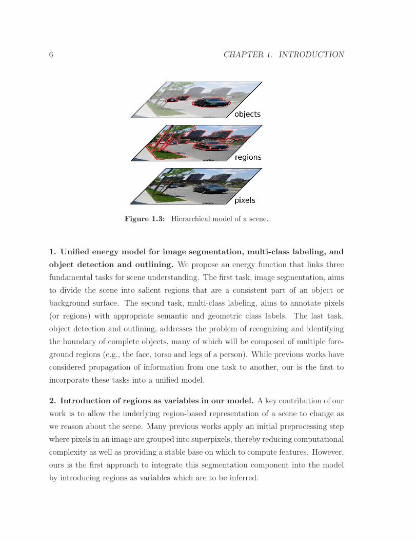
Figure 1.2 illustrates the three different tasks that we aim to unite in this thesis.
The first task (in Figure 1.2(b)) aims to divide the scene into regions and labels each

4 CHAPTER 1. INTRODUCTION
(a) Image (b) Regions
(c) Objects (d) Geometry
Figure 1.2: Illustration of the aim of this thesis to understanding outdoor scenes in termsof regions, objects and geometry.
one with a semantic class label. We call this task scene decomposition. It is similar
to pixel labeling, which assigns a label to each pixel, but in addition groups pixels
into coherent regions so that two adjacent pixels can have the same class label but
be grouped into different regions, thereby separating adjacent objects of the same
class. As we shall discuss in Chapter 4, there are many different ways in which a
scene can be decomposed. For example, we could naively treat each pixel as its own
region. For now, it is sufficient for us to loosely define scene decomposition to be the
segmentation of an image into semantically and geometrically consistent regions with
respect to a predefined set of possible labels. In our work, this label set includes a
1.1. CONTRIBUTIONS 5
generic object label for modeling the wide variety of foreground object classes that
we are likely to encounter.
The second task, shown in Figure 1.2(c), is in some sense an enhancement of the
first. Here, we would like to refine generic class labels, such as object, into specific
categories, and identify individual instances of these categories. The last task (shown
in Figure 1.2(d)) involves understanding the 3D structure of the scene, including the
location of the horizon and the relative placement of objects and dominant back-
ground regions. It is only, by understanding all three aspects—regions, objects and
geometry—that we can really claim to have understood the scene. Of course, there
are other tasks that can build on these (e.g., activity recognition), and we will discuss
some of these as future research directions in Chapter 7.
This thesis contributes to bridging the gap between low-level image representa-
tion (i.e., pixels) and high-level scene understanding in terms of regions, objects and
geometry. As discussed above, our aim is to decompose a scene into semantic and
geometrically consistent regions. Each region is annotated with a semantic and ge-
ometric class labels. From this region-level description of the scene we will progress
to identifying the objects in the scene and its geometry. This hierarchical model,
illustrated in Figure 1.3, shares much in common with early computer vision systems
which attempted to fully interpret the scene (e.g., [Ohta et al., 1978]). However, un-
like these early feed-forward systems, our framework allows feedback from high-level
scene entities to the low-level decomposition. Specifically, our model is holistic and we
allow probabilistic influence to flow in both directions. Furthermore, the parameters
of our models are learned from data allowing us to consider many more features and
making our models more robust.
The following section summarizes our main contributions. We then provide a brief
outline for the remainder of this dissertation and contrast our research with related
work in the field.
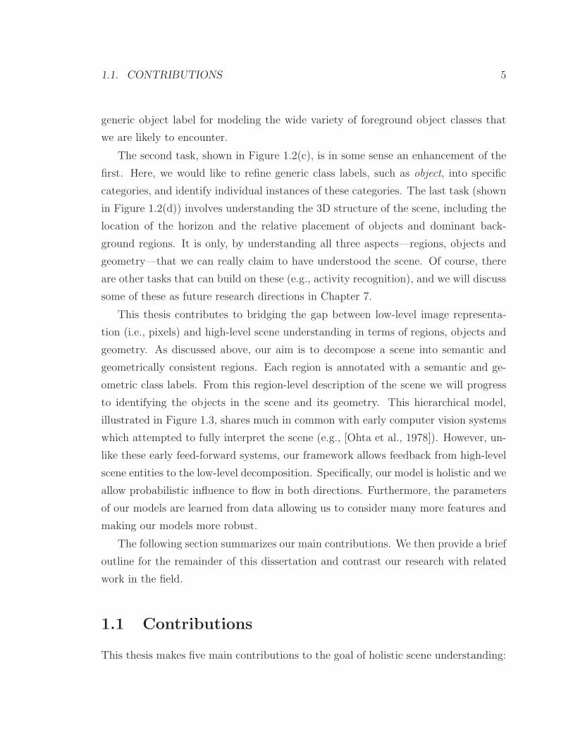
1.1 Contributions
This thesis makes five main contributions to the goal of holistic scene understanding:
6 CHAPTER 1. INTRODUCTION
Figure 1.3: Hierarchical model of a scene.
1. Unified energy model for image segmentation, multi-class labeling, and
object detection and outlining. We propose an energy function that links three
fundamental tasks for scene understanding. The first task, image segmentation, aims
to divide the scene into salient regions that are a consistent part of an object or
background surface. The second task, multi-class labeling, aims to annotate pixels
(or regions) with appropriate semantic and geometric class labels. The last task,
object detection and outlining, addresses the problem of recognizing and identifying
the boundary of complete objects, many of which will be composed of multiple fore-
ground regions (e.g., the face, torso and legs of a person). While previous works have
considered propagation of information from one task to another, our is the first to
incorporate these tasks into a unified model.
2. Introduction of regions as variables in our model. A key contribution of our
work is to allow the underlying region-based representation of a scene to change as
we reason about the scene. Many previous works apply an initial preprocessing step
where pixels in an image are grouped into superpixels, thereby reducing computational
complexity as well as providing a stable base on which to compute features. However,
ours is the first approach to integrate this segmentation component into the model
by introducing regions as variables which are to be inferred.

1.2. THESIS OUTLINE 7
3. Efficient inference. One of the major difficulties with holistic models of vision is
the significant burden placed on the inference procedure to deal with the interactions
between model components. We address this problem by developing an efficient
inference procedure that makes large moves in energy space. This approach allows
our algorithm to find good approximate solutions of the energy function.
4. Incorporation of semantics as an aid for 3D scene reconstruction. We
propose an approach to recovering the 3D layout of a scene that makes use of seman-
tic content. Specifically, we use predicted semantic labels and region boundaries as
context for depth reconstruction. Unlike previous approaches, this allows us to ex-
ploit class-related geometric priors and better model the relationship between region
appearance and depth.
5. Development of scene dataset and annotation tools. As part of the de-
velopment of the algorithms described in this thesis, we collected a large dataset of
outdoor scenes and developed software tools for annotating these scenes with semantic
and geometric information. The software tools allow us to leverage the Amazon Me-
chanical Turk (AMT) online workforce to obtain high-quality labeled images cheaply
and rapidly.
1.2 Thesis Outline
The remaining chapters of this thesis are summarized below:
Chapter 2: Background. This chapter includes the basic technical background and
notation needed to understand the remainder of the thesis. The chapter is divided
into two main sections. In the first section, we discuss the machine learning and
probabilistic modeling techniques used in our work. The second section provides a
review of image formation, standard image features, and state-of-the-art techniques
for high-level computer vision, in particular, object detection and multi-class image
labeling.

8 CHAPTER 1. INTRODUCTION
Chapter 3: Image datasets and dataset construction. In this chapter we dis-
cuss the various publicly available datasets used in the computer vision community
and highlight the ones used for evaluating our work. Many of the datasets are de-
veloped with a particular task in mind, and we discuss their suitability to the scene
understanding task. We then introduce a new dataset that includes both semantic
and geometric labels and describe an online annotation tool that we developed for
constructing this dataset.
Chapter 4: Scene decomposition: from pixels to regions. In this chapter we
present our model for decomposing a scene into semantic and geometrically consistent
regions. We describe our representation for the entities of the scene—pixels, regions,
and geometry—over which we wish to reason. We then present our unified energy
function for scoring different decompositions of a scene and describe methods for
learning and performing approximate inference on this energy function.
Chapter 5: Object detection and outlining: from regions to objects. Build-
ing on the scene decomposition framework of Chapter 4, we introduce the notion of
objects into our model. Here, our objective is to identify and outline known objects,
each of which can be composed of one or more foreground regions. We show how
our unified energy function can be extended to support this objective and discuss a
modification to our inference procedure that improves efficiency.
Chapter 6: Scene reconstruction: from semantics to geometry. In this
chapter, we discuss models for 3D reconstruction of a scene given a decomposition into
semantically labeled regions. We first show how a basic geometric reconstruction can
be produced by “popping up” vertical regions from a supporting ground plane. Next,
we discuss a model for metric reconstruction in which we perform depth perception
aided by our semantic understanding.
Chapter 7: Conclusions and future directions. We conclude the thesis with a
summary of our main contributions and discussion of future directions for improving
our work.
1.3. RELATED WORK 9
Appendix A: Implementation details. Here we discuss some implementation
details necessary for efficient feature computation and inference.
1.3 Related Work
Our work builds on recent advances in many areas of computer vision and machine
learning, for example, multi-class image labeling [He et al., 2004, Kumar and Hebert,
2005, Shotton et al., 2006], object detection and recognition [Torralba et al., 2004a,
Dalal and Triggs, 2005, Opelt et al., 2006a, Viola and Jones, 2004], and geometric
reasoning [Criminisi et al., 2000, Hoiem et al., 2007a, Saxena et al., 2008]. While these
works only attempt to interpret part of the scene, they all provide insights and con-
tribute results which we leverage. As we will discuss, we also share common features
with other works that attempt a more complete interpretation of the scene [Heitz
et al., 2008b, Hoiem et al., 2008a, Li et al., 2009].
Early Work in Scene Understanding. We begin with a discussion of some early
work in scene understanding. Researchers, inspired by the study of biological systems,
developed a computational theory of vision [Marr, 1982, Barrow and Tenenbaum,
1981] that supported a feed-forward model where low-level inputs are combined into
higher and higher level structures. One approach was to move from a primal sketch
of the scene, in which an image is decomposed into edges and regions, to a full
3D interpretation (including recognition of objects and their geometric arrangement
within the scene).
This ambitious full-scene approach to computer vision was demonstrated by a
number of early systems that attempted to combine bottom-up processing with
higher-level modeling. Such full scene interpretation systems included the segment
merging approach of Ohta et al. [1978], the VISIONS system of Hanson and Riseman
[1978], and the geometric primitives approach (ACRONYM) of Brooks [1983]. Unfor-
tunately, these early systems were brittle due to many issues, including hand-coding
of parameters and limited computational resources. Attempts at holistic scene un-
derstanding were soon abandoned in favor of more tractable tasks such as shape from
10 CHAPTER 1. INTRODUCTION
shading [Horn, 1989], edge detection [Canny, 1986], and recognition of specific object
categories, e.g., faces [Viola and Jones, 2001].
There were also many early attempts to solve subtasks in computer vision by
narrowing the range of inputs to the problem. Perhaps the most famous of these
is the work of Waltz [1975], which aims to automatically elicit the 3D structure of
a scene from line drawings. Waltz’s algorithm begins by extracting the corners and
junctions from the image, and then attempts to label these and the edges between
them to indicate geometry (e.g., concave, convex, occluding, etc.). From this labeling,
a 3D reconstruction of the scene could be produced. A key contribution of Waltz
[1975] was to enforce consistency in the labeling of edges and junctions, and the work
became the cornerstone for a large and important body of algorithms that solve so-
called constraint satisfaction problems (CSPs).1 However, clean line drawings are a
significant simplification of real-world scenes, and unfortunately, Waltz’s algorithm
was unable to meet to the challenges of natural scenes.
Many of the ideas developed in these early works are being revisited in con-
temporary research. What is remarkable is that, with improved machine learning
techniques, computational power, and availability of large amounts of data, the ideas
are producing fruitful results. That is, the early computer vision researchers had the
right insights, but not the right tools to make their ideas successful.
Multi-class Image Segmentation. Turning to more recent times, the problem of
multi-class image segmentation (or pixel labeling) has been successfully addressed by
a number of works [He et al., 2004, Shotton et al., 2006, Ladicky et al., 2009]. The
goal of these works is to label every pixel in the image with a single class label from
a fixed predefined set. Typically, these algorithms construct conditional Markov ran-
dom fields (CRFs) over the pixels (or small coherent regions called superpixels) with
local class-predictors, based on pixel appearance, and a pairwise smoothness term to
encourage neighboring pixels to take the same label. The works differ in the details
of the energy functions and the inference algorithms used. For example, Ladicky
et al. [2009], in addition to using very sophisticated features, take the innovative step
1Constraint satisfaction problems are closely related to the Markov random fields (MRFs) thatwe use in our work to enforce soft, rather than hard, constraints.

1.3. RELATED WORK 11
of encouraging label consistency over large contiguous regions (known as superpixel)
through the use of high-order energy terms. However, none of the works aim to sepa-
rate instances of the same object class. In these approaches a crowd of people will be
labeled as a single contiguous “person” region rather than delineating the individual
people.
Some novel works introduce 2D layout consistency between objects [Winn and
Shotton, 2006] or object shape [Winn and Jojic, 2005, Kumar et al., 2005, Yang et al.,
2007] in an attempt to segment out foreground objects. These, and other attempts at
figure-ground segmentation [Rother et al., 2004, Boykov and Jolly, 2001, Mortensen
and Barrett, 1998, Borenstein and Ullman, 2002, Leibe et al., 2004, Levin and Weiss,
2006, Winn et al., 2005], work well when objects have a distinct shape (or appearance)
and are well-framed (i.e., large and centered) within the image. However, many of
the scenes that we consider contain small objects—a domain not suited to these
approaches. Furthermore, these approaches do not attempt to label the background
regions which we require for context and geometry.
In addition to layout consistency and shape, some researchers have explored rela-
tive location and co-occurrence between regions [Rabinovich et al., 2007, Gould et al.,
2008, Lim et al., 2009]. For example, Rabinovich et al. [2007] learn the number of
times different object classes appear together in the same image, and use that in-
formation to constrain pixel labelings in novel images. Gould et al. [2008] explore
context-dependent relative location priors as a means of enforcing spatial arrange-
ment of classes. For example, the relative location priors model that cows tend to be
surrounded by grass (in 2D images). None of these works, however, take into account
the 3D arrangement of a scene and do not learn to enforce global consistency, such
as that “sky” needs to be above “ground”.
Liu et al. [2009] use a non-parametric approach to image labeling by warping a
novel image onto a large set of labeled images with similar appearance. The method
then copies the (warped) labels and combines them using a CRF model to obtain a
labeling for the novel image. This is a very effective approach since it scales easily
to a large number of classes. However, the method does not attempt to understand
the scene semantics. In particular, their method is unable to break the scene into

12 CHAPTER 1. INTRODUCTION
separate objects (e.g., a row of cars will be parsed as a single region) and cannot
capture combinations of classes not present in the training set. As a result, the
approach performs poorly on most foreground object classes.
The use of multiple different over-segmented images (i.e., superpixels) as a pre-
processing step is not new to computer vision. Russell et al. [2006], for example,
use multiple over-segmentations for finding objects in images, and many of the depth
reconstruction methods described below (e.g., [Hoiem et al., 2007a]) make use of over-
segmentations for computing feature statistics. In the context of multi-class image
segmentation, Kohli et al. [2008] specify a global objective which rewards solutions
in which an entire superpixel is labeled consistently. However, their energy function
is very restricted and does not, for example, capture the interaction between region
appearance and class label, nor does their energy function allow for label-dependent
pairwise preferences, such as foreground objects above road. Their approach was
extended in Ladicky et al. [2009] to handle the first of these deficiencies, but not
the second. Unlike all of these methods that use multiple over-segmented images,
our method uses multiple over-segmentations to build a dictionary of proposal moves
for optimizing a global energy function—the segments themselves are not used for
computing features nor do they appear explicitly in our objective.
Image Parsing. As an extension to multi-class image segmentation, there has also
been some recent work on image parsing [Tu et al., 2003, 2005, Han and Zhu, 2009].
Here, the aim is to decompose the image into a single hierarchical segmentation
describing the scene. Such a representation would allow, for example, a segmentation
that understands both car objects as a whole and wheels as parts of cars. These
methods point to promising future results. However, they are currently still in their
infancy and are, as yet, unable to explain the whole scene. For example, the work
of Tu et al. [2003, 2005] demonstrates effective segmentation of a scene into face and
text regions, but does not attempt to understand the remaining areas in the image.
Han and Zhu [2009] define a parse grammar for understanding man-made scenes
(e.g., buildings) and generate a top-down parse of the scene into primitives defined
by this grammar. Their approach shares many ideas with some early approaches

1.3. RELATED WORK 13
to scene understanding (e.g., [Ohta et al., 1978, Brooks, 1983]), but using modern
machine learning techniques. Currently, the system only works on highly structured
scenes consisting of mainly rectangular elements. Furthermore, Han and Zhu [2009]
focus on extracting scene geometry and make no attempt to understand the scene’s
semantics.
Object Detection. Object detection is one of the most heavily studied topics in
computer vision and much progress has been made in recent years [Viola and Jones,
2004, Brubaker et al., 2007, Fergus et al., 2003, Torralba et al., 2004a, Dalal and
Triggs, 2005, Opelt et al., 2006a, Fei-Fei et al., 2006, Felzenszwalb et al., 2010]. The
vast majority of works use localized cues extracted from within candidate object
bounding boxes to find and classify objects. The highly successful approach of Dalal
and Triggs [2005], for example, uses the orientation of edges extracted from overlap-
ping cells within the candidate bounding box to build up a descriptor for classifying
the object. The state-of-the-art work of Felzenszwalb et al. [2010] builds on this ap-
proach by extracting these same features at two resolutions, one for the whole object
and one for object parts (which are free to deviate slightly from their nominal posi-
tions within the bounding box for the whole object). All of these methods attempt to
understand the scene as a collection of independent objects and do not consider other
aspects of the scene (e.g., background regions). They do form incredible powerful
building blocks for holistic scene understanding, however, and we make extensive use
of the tools developed along this line of research in Chapter 5.
A number of researchers have suggested the importance of context in object detec-
tion [Divvala et al., 2009, Galleguillos and Belongie, 2008, Torralba et al., 2006]. The
empirical study of Divvala et al. [2009] showed that many different sources of context
can be leveraged to improve object detection performance, including scene level con-
text (i.e., certain objects are more likely to occur within certain scene types), object
size, object location, and spatial support. Some previous works have also made at-
tempts at incorporating contextual information for improving object detection [Fink
and Perona, 2003, Torralba et al., 2004b, Murphy et al., 2003, Heitz and Koller, 2008,
Tu, 2008]. However, the majority of these works incorporate feature-level context
14 CHAPTER 1. INTRODUCTION
(e.g., neighborhood appearance) rather than semantic or geometric context.
A notable exception is the work of Hoiem et al. [2006], which relates global scene
geometry (i.e., camera pose) to object size. This enforces consistency between the
height of detected objects, allowing some false positives to be rejected. The approach
requires a number of well detected objects to be present in the scene in order to get
a good estimate of camera pose. Moreover, in cluttered environments (e.g., urban
scenes) many “in-context” false positives will remain.
Other works attempt to integrate tasks such as object detection and multi-class
image segmentation into a single CRF model. However, these models either use a
different representation for object and non-object regions [Wojek and Schiele, 2008] or
rely on a pixel-level representation [Shotton et al., 2006]. The former does not enforce
label consistency between object bounding boxes and the underlying pixels while the
latter does not distinguish between adjacent objects of the same class. Recent work
by Yang et al. [2010] performs joint reasoning over objects and their segmentations
in a unified probabilistic model. However, they are only concerned with foreground
object segmentations and do not explain the full scene or its geometry.
Recent work by Gu et al. [2009] uses regions for object detection instead of the tra-
ditional sliding-window approach. However, unlike the method that we develop in this
thesis, they use a single over-segmentation of the image and make the strong assump-
tion that each segment represents a probabilistically recognizable object part. Our
method, on the other hand, assembles objects and background regions using segments
from multiple different over-segmentations. The multiple over-segmentations avoids
errors made by any one segmentation. Furthermore, we incorporate background re-
gions which allows us to eliminate large portions of the image thereby reducing the
number of component regions that need to be considered for each object.
Geometric Reasoning and 3D Structure. We can roughly partition methods
that attempt to explain the 3D structure of an entire scene into two groups: geo-
metric models and depth perception models. For indoor environments, Delage et al.
[2006] use an MRF for reconstructing the location of walls, ceilings, and floors using
geometric cues (such as long straight lines) derived from the scene. More recently,

1.3. RELATED WORK 15
Hedau et al. [2009] recover the spatial layout of cluttered rooms using similar geo-
metric cues. Both models make strong assumptions about the structure of indoor
environments (such as the “box” model of a room [Hedau et al., 2009]) and are not
suitable to the less structured outdoor scenes that we consider.
An early approach to outdoor scene reconstruction is the innovative work of Hoiem
et al. [2005b] who cast the problem as a multinomial classification problem similar
in spirit to the multi-class image labeling works discussed above. In their work, pix-
els are classified as either ground, sky, or vertical. A simple 3D model can then be
constructed by “popping up” vertical regions. The model was later improved [Hoiem
et al., 2007a] to incorporate a broader range of geometric subclasses (porous, solid,
left, center, right). These models make no attempt to estimate absolute depth. Fur-
thermore, many objects commonly found in everyday scenes (e.g., cars, trees, and
people) do not neatly fit into the broad classes they define. A car, for example,
consists of many angled surfaces that cannot be modeled as vertical.
It is interesting to note the connection between background semantic classes and
the geometric subclasses defined by Hoiem et al. [2007a]: trees are generally porous;
buildings are vertical; and road, grass and water are horizontal. Indeed, our own
scene decomposition model (discussed in Chapter 4) exploits the strong correlation
between geometry and semantics in outdoor scenes.
In related work, Hoiem et al. [2007b], attempt to infer occlusion boundaries within
images. The success of their approach hinges on the quality of the geometric cues
obtained from the pixel labeling model just discussed [Hoiem et al., 2007a]. By similar
construction to the pixel labeling work, a “pop up” of the scene can be generated.
An interesting feature of this work is that it makes use of the constraint satisfaction
algorithm of Waltz [1975] discussed previously.
A more semantically motivated approach to depth reconstruction was recently
adopted by Russell and Torralba [2009] who utilize detailed human-labeled segmen-
tations to infer the geometric class of regions (ground, standing, attached) and region
edges (support, occlusion, attachment). In their model, depth inference is done by
modeling support and attachment relationships relative to a ground plane. Currently,
their model relies on detailed human annotation of regions, and in particular, their

16 CHAPTER 1. INTRODUCTION
polygonal boundaries, within the scene.
Our depth estimation work (discussed in Chapter 6) is most heavily influenced by
the work of Saxena and colleagues [Saxena et al., 2008, 2005] who take a very different
approach to the task of 3D reconstruction. Instead of inferring geometric class labels,
they infer the absolute depth of the pixels in the image. However, unlike their ap-
proach, which completely ignores semantic context, our work makes use of semantic
information (i.e., region boundaries and class labels) to guide depth perception. This
has a number of advantages: First, we can use simpler features since depth perception
in our model is conditioned on semantic class and thus avoids the need for features
that correlate with depth across all classes. Second, we avoid the need for modeling
occlusions and folds since these can be easily obtained from the region boundaries and
associated semantic labels (sky is always occluded; ground plane classes “fold” into
foreground classes). Last, co-planarity and connectivity constraints can be imposed
differently within each semantic class. For example, a building is more likely to be
planar than a tree.
Holistic Scene Understanding. None of the above methods directly tackle the
problem of describing the entire scene and all restrict themselves to annotating either
semantic components or geometric components, but not both. A few recent works
have begun to re-explore the ideas of the early computer vision researchers and develop
holistic models for scene understanding [Heitz et al., 2008b, Hoiem et al., 2008a, Li
et al., 2009]. These works aim to leverage correlations between different aspects of a
scene to improve performance across the different tasks.
Heitz et al. [2008b] made one of the first attempts by combining scene catego-
rization, object detection, image segmentation, and depth information into a single
model. Significant improvements was demonstrated by propagating information from
one task to another through a cascade of repeated models. However, no consistency
was enforced in the final output generated by the cascade, and the lower layers simply
act to provide strong additional features to subsequent layers in the cascade.
In a similar attempt, Hoiem et al. [2008a] propose a system for integrating the
tasks of object recognition, surface orientation estimation, and occlusion boundary

1.4. PREVIOUSLY PUBLISHED WORK 17
detection. Like the model of Heitz et al. [2008b], their system is modular and leverages
state-of-the-art components. And similarly, consistency is not enforced in the final
output.
Li et al. [2009] also develop a holistic model of a scene that enforces label consis-
tency between tasks. In their work, classification, segmentation, and textual annota-
tion, are combined within a single model. Their model explains the whole scene, but
in order to make inference tractable, they do not model spatial constraints. Further-
more, their work makes no attempt to distinguish between multiple instances of the
same object category in the image.
The success of these contemporary holistic scene understanding models has been
a key motivation for our work. However, unlike these approaches, we desire a model
that produces a coherent labeling of the scene, identifies distinct object instances,
and interprets the scene geometry.
1.4 Previously Published Work
Much of the work described in this thesis has been previously published in conference
proceedings. In particular, our scene decomposition model and inference procedure
(described in Chapter 4), in which we decompose a scene into semantic and geomet-
rically consistent regions, was published in Gould et al. [2009b]. A brief discussion of
the dataset and image annotation pipeline using Amazon Mechanical Turk (AMT)
appears in this work. We provide a more complete description in Chapter 3.
An early version of the extension to our scene decomposition model for recogniz-
ing and outlining foreground objects (described in Chapter 5) was published in Gould
et al. [2009c]. However, experiments on the CCM dataset have not appeared previ-
ously. Finally, our model for reconstructing the 3D geometry of a scene from a se-
mantic decomposition (described in Chapter 6) first appeared in Gould et al. [2009b],
and was later expanded to include depth perception in Liu et al. [2010]. This thesis
further extends that work.

18 CHAPTER 1. INTRODUCTION

Chapter 2
Background
The work in this thesis is built on the foundations of two large fields of study—
computer vision (CV) and machine learning (ML). Indeed, these fields are now very
much integrated: Much of modern computer vision (at least, high-level computer
vision) incorporates machine learning techniques so that algorithms can make use of
data for training parameters rather than setting them manually, thereby accelerating
development and hopefully making the algorithms more. Likewise, many machine
learning techniques are motivated by problems arising in computer vision and then
applied more broadly. The purpose of this chapter is to provide a very brief introduc-
tion to these two fields. The chapter is not intended to be a comprehensive treatment
of either computer vision or machine learning. For an in depth coverage of the topics
covered in this chapter, the reader should consult one of the excellent textbooks on
machine learning (e.g., [Koller and Friedman, 2009, Duda et al., 2000, Bishop, 1996,
2007, Hastie et al., 2009]) or computer vision (e.g., [Forsyth and Ponce, 2002, Ma
et al., 2005, Hartley and Zisserman, 2004, Trucco and Verri, 1998]).
2.1 Machine Learning and Graphical Models
Machine learning is a large and diverse field concerned with the development of al-
gorithms that adapt themselves based on observed data. In this thesis we will be
19

20 CHAPTER 2. BACKGROUND
concerned with supervised learning, which deals with the problem of learning a map-
ping from features to outputs (i.e., labels or distributions over labels) given a set of
training exemplars. In our work, the features are represented by n-dimensional real-
valued vectors x ∈ Rn. The labels y can either be continuous, discrete, or structured
(i.e., vector-valued with dependencies between the outputs). We will use the nota-
tion y ∈ Y to denote that y can take its value from the discrete set Y. The machine
learning framework learns a classification (or regression) function f : Rn → Y or
probability distribution P (Y |X).
The supervised learning paradigm, typically, contains the following steps:
• Data collection and partitioning. Data instances are acquired and labeled.
The data is usually then split into training and testing sets.
• Feature extraction. Feature vectors x ∈ Rn are extracted from the data
instances.
• Parameter learning. A parametric model is selected and the parameters θ
learned with respect to an objective over the training set D = (x(i), y(i))Ni=1.
• Evaluation. The performance of the model is evaluated on the set of test in-
stances. The performance metric need not match the training objective (usually
due to the intractability of training with the true objective).
The above procedure is usually repeated with different folds of the data, that is,
different partitioning into training and testing sets to get a measure of the algorithm’s
sensitivity to changes in training/testing sets.
In the following section we will provide an overview of machine learning algorithms
for classification and regression. In Section 2.1.2 we describe probabilistic graphical
models that allow us to efficiently model probability distributions over structured
data (i.e., multi-valued output).
2.1.1 Classification and Regression
In this section we discuss regression (continuous-valued output spaces) and classifi-
cation (discrete-valued output spaces) models that we use in this thesis.
2.1. MACHINE LEARNING AND GRAPHICAL MODELS 21
Linear Regression
Regression aims to predict (or model) a continuous-valued target variable. The most
simple type of regression is linear regression. Here, we assume that our target variable
y ∈ R can be modeled as a linear combination of features, that is, y = θT x+ η where
η is some unknown random noise (usually assumed to be zero-mean Gaussian). The
parameters θ ∈ Rn are estimated by minimizing a cost function over the training set
D = (x(i), y(i))Ni=1. A very common cost function is the sum-of-squares residual,
giving rise to the optimization problem,
minimize (over θ)
N∑
i=1
(y(i) − θT x(i)
)2(2.1)
which can be solved in closed-form to give θ⋆ =(∑N
i=1 x(i)(x(i))T)−1 (∑N
i=1 y(i)x(i)
)
.
In our work on depth estimation, we will use a more robust cost function that is
less sensitive to outliers. Specifically, we solve the optimization problem,
minimize (over θ)N∑
i=1
h(y(i) − θT x(i);β
)(2.2)
where h(x;β) is the Huber penalty defined as
h(x;β) =
x2 for −β ≤ x ≤ β
β(2|x| − β) otherwise.(2.3)
The optimization problem in Equation 2.2 has no closed-form solution, but the ob-
jective function is convex and usually solved using a quasi-newton technique [Boyd
and Vandenberghe, 2004]. To prevent over-fitting, a regularization penalty on the
parameters, λr(θ), can be added to the objective, where λ ≥ 0 controls the strength
of the regularization, and r(θ) is the regularization function (or prior). A typical
choice for the regularization function is the ℓ2-regularizer, r(θ) = ‖θ‖22, which keeps
the problem convex.

22 CHAPTER 2. BACKGROUND
Logistic Regression Models
Multi-class logistic regression (sometimes called softmax regression) is a parametric
probability distribution often used for discriminative classification. The model defines
a probability distribution over a discrete random variable Y and observed features
x ∈ Rn as
P (Y = y |X = x;θ) =exp
(θT
y x)
∑
y′∈Y exp(θT
y′x) (2.4)
where θ ∈ Rn×|Y| are the parameters of the model.1 In our work, we will often use a
quadratic kernel function on the raw features by augmenting x with the product of
all pairs of features, i.e., x′ = (x1, . . . , xn, x21, . . . , xixj, . . . , x
2n), where for all pairwise
terms xixj we have j ≥ i. This allows more expressive models to be learned by
considering pairwise correlations between the features.
In general, we can replace the observed features x in Equation 2.4 with a joint
feature function over both features and labels, i.e., φ(y,x) ∈ Rm where φ : Y ×R
n →R
m. In this case the multi-class logistic model can be rewritten as
P (Y = y |X = x; θ) =exp
(θTφ(y,x)
)
∑
y′∈Y exp (θTφ(y,x))(2.5)
where θ ∈ Rm are the parameters of the model. In this form, the standard multi-class
logistic model (Equation 2.4) has joint feature function
φ(y,x) = (1y = 1x, . . . ,1y = Kx) (2.6)
for label set Y = 1, . . . ,K. Here, 1P is the indicator function (or Iverson bracket)
taking the value one if P is true, and zero otherwise. This joint feature representation
allows more general interactions between features and labels to be encoded, and will be
useful when we introduce conditional Markov random fields (CRFs) in Section 2.1.2.
The multi-class logistic regression model can be used as a discriminative classifier
1Note that this is an over-complete parameterization. Often the parameters for the last classlabel are fixed to zero, i.e., θ|Y| = 0n.

2.1. MACHINE LEARNING AND GRAPHICAL MODELS 23
by taking the most likely assignment to the output according to the model, i.e., y =
argmaxyP (y | x). In our work, however, we use the multi-class logistic as a component
within our CRF models for scoring local variable configurations.
Most often, the parameters of the multi-class logistic are learned according to a
maximum-likelihood objective (on the training set) with regularization on the param-
eters to control overfitting, i.e.,
maximize (over θ)∑N
i=1 log P(y(i) | x(i);θ
)− λr(θ) (2.7)
where λ ∈ R+ is the regularization constant and r(θ) is the regularization function
(or prior). As with linear regression, a typical choice for the regularization function
is the ℓ2-regularizer, r(θ) = ‖θ‖22. The objective in Equation 2.7 is concave (as long
as r(θ) is convex) admitting efficient computation of the optimal parameters.
Boosted Classifiers
Boosting [Freund and Schapire, 1995] is another popular approach to learning dis-
criminative classifiers. Here, many weak learners are combined into a single strong
classifier. The algorithm has many variants and we only describe the most basic
variant in this section. We will assume that our problem is a binary classification
problem with label space Y = −1, 1. Each weak learner constructs a classifier from
features to labels, i.e., ht : Rn → −1, 1. In our work, we will assume that the
weak learners are decision trees [Hastie et al., 2009]. The algorithm for learning the
strong classifier f : Rn → R is given in Algorithm 2.1. Classification is performed as
y = sign (f(x)). This algorithm can be shown to minimize the exponential training
loss [Friedman et al., 1998].
As mentioned, there are many variants of the boosting, including extensions to
multi-valued and continuous label spaces. In this thesis we use the GentleBoost [Fried-
man et al., 1998] variant of boosting (which sets αt = 1 in line 12 of Algorithm 2.1)
for learning pixel-wise semantic features.
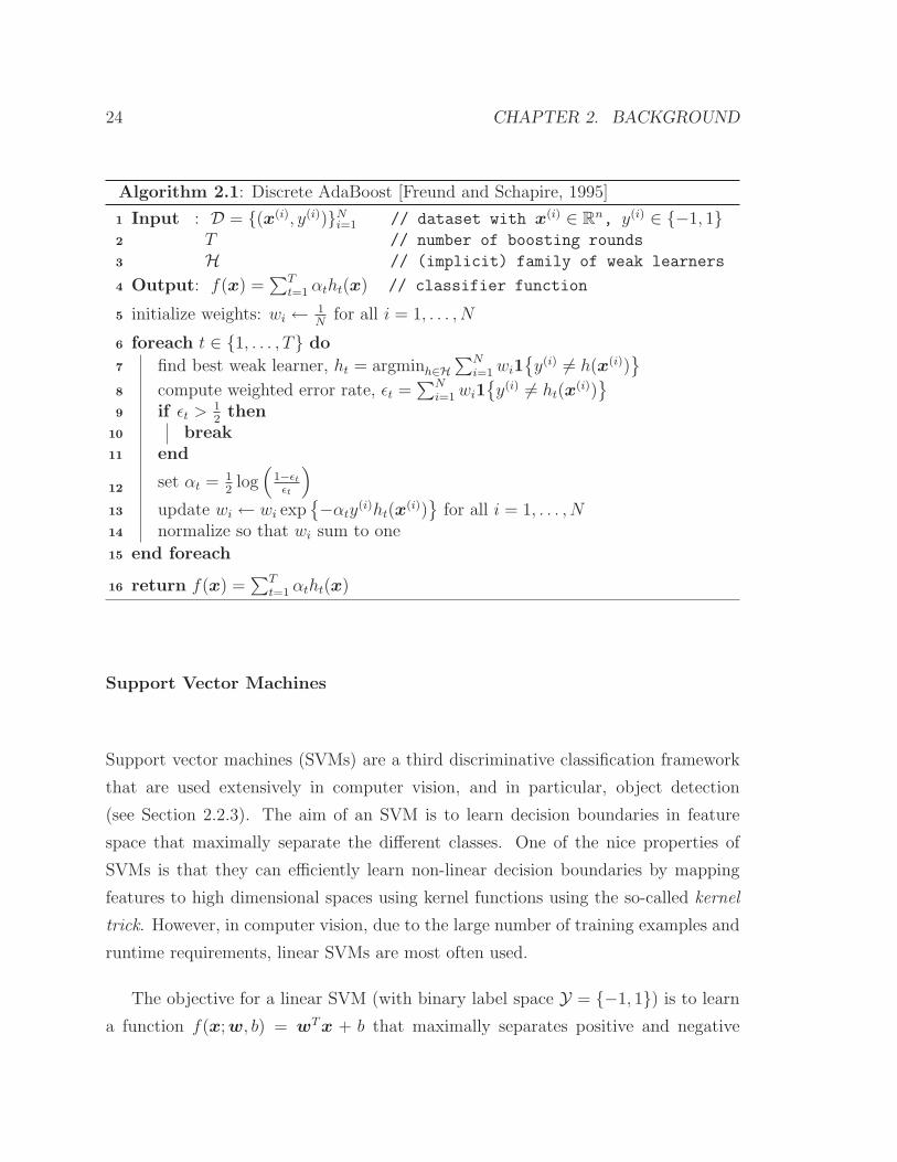
24 CHAPTER 2. BACKGROUND
Algorithm 2.1: Discrete AdaBoost [Freund and Schapire, 1995]
Input : D = (x(i), y(i))Ni=1 // dataset with x(i) ∈ Rn, y(i) ∈ −1, 11
T // number of boosting rounds2
H // (implicit) family of weak learners3
Output: f(x) =∑T
t=1 αtht(x) // classifier function4
initialize weights: wi ← 1N
for all i = 1, . . . , N5
foreach t ∈ 1, . . . , T do6
find best weak learner, ht = argminh∈H
∑N
i=1wi1y(i) 6= h(x(i))
7
compute weighted error rate, ǫt =∑N
i=1wi1y(i) 6= ht(x
(i))
8
if ǫt >12
then9
break10
end11
set αt = 12log(
1−ǫt
ǫt
)
12
update wi ← wi exp−αty
(i)ht(x(i))
for all i = 1, . . . , N13
normalize so that wi sum to one14
end foreach15
return f(x) =∑T
t=1 αtht(x)16
Support Vector Machines
Support vector machines (SVMs) are a third discriminative classification framework
that are used extensively in computer vision, and in particular, object detection
(see Section 2.2.3). The aim of an SVM is to learn decision boundaries in feature
space that maximally separate the different classes. One of the nice properties of
SVMs is that they can efficiently learn non-linear decision boundaries by mapping
features to high dimensional spaces using kernel functions using the so-called kernel
trick. However, in computer vision, due to the large number of training examples and
runtime requirements, linear SVMs are most often used.
The objective for a linear SVM (with binary label space Y = −1, 1) is to learn
a function f(x;w, b) = wT x + b that maximally separates positive and negative

2.1. MACHINE LEARNING AND GRAPHICAL MODELS 25
training examples. Specifically, the training objective is
minimize (over w, b, ξ) 12‖w‖2 + C
∑N
i=1 ξi
subject to y(i)(wT x(i) + b
)≥ 1− ξi, i = 1, . . . , N
ξi ≥ 0, i = 1, . . . , N
(2.8)
where C is a parameter that controls the trade-off between maximizing the margin
and separating the positive and negative examples (which may not always be linearly
separable).
The basic SVM framework can be extended for the structured prediction task,
where Y = Y1 × · · · × Yn is an output space over many interacting variables, but we
do not consider this extension when learning models in this thesis.
2.1.2 Probabilistic Graphical Models
Probabilistic graphical models [Koller and Friedman, 2009] are a powerful framework
that combines probability theory and graph theory for modeling probability distri-
butions over large structured output spaces. Two key benefits of graphical models
(over an explicit representation of the joint probability distribution) is that they can
be represented compactly and induce efficient algorithms for (approximate) inference
and learning. This is achieved by representing the probability distribution over a set
of random variables Y = (Y1, . . . , Yn) in a factored form:
P (Y1, . . . , Yn) =1
Z
∏
c∈C
Ψc(Y c) =1
Zexp
−∑
c∈C
ψc(Y c)
(2.9)
where C are a set of cliques in the graph and Z is the so-called partition function
that ensures that the probability distribution sums to one. The functions Ψc(Y c) are
called potential functions and define a local model over the subset of the variables
Y c ⊆ Y in the c-th clique.
There are many different flavors of graphical models and in this thesis we will
focus on models known as conditional Markov random fields.
26 CHAPTER 2. BACKGROUND
Conditional Markov Random Fields
Conditional Markov random fields (CRFs) are a type of probabilistic graphical model
originally introduced by Lafferty et al. [2001] in the context of natural language
processing, but now commonly used for many other problems, including computer
vision and computational biology. Concretely, a CRF defines a model over a finite
set of random variables Y = (Y1, . . . , Yn) and observed features X. In the context
of scene understanding, the observations X represent the image features extracted
from the image and the random variables Y represent the entities over which we
are reasoning (e.g., semantic labels for the pixels). Each random variable Yi can be
assigned a value from some (discrete) value space Yi, e.g., the semantic label for a
region can be sky, road, grass, etc. The joint assignment to all random variables
is denoted by y ∈ Y where Y ⊆ Y1 × · · · × Yn is the space of all possible joint
assignments. The general form of a CRF is then
P (Y = y |X = x) =1
Z(x)exp
−∑
c
ψc(yc;x)
(2.10)
where each term ψc(yc;x) is defined over a subset, or clique, of random variables
Y c ⊆ Y and yc ∈ Yc represents the corresponding assignment to these variables.
The terms are known as (log-space) clique potential or factors. Formally, we have
the potential ψc : Yc ×X → R defining a preference for assignments to the subset of
random variables Y c given the observations X. The sum over potential functions is
called the energy function and is denoted E (y;x) =∑
c ψc(yc;x). The term Z(x) is
a normalization constant (partition function) that ensures the probability distribution
sums to one, i.e.,
Z(x) =∑
y∈Y
exp −E (y;x) . (2.11)
A simple example of a pairwise CRF over four random variables is shown in
Figure 2.1(a). The graphical structure denotes direct dependencies between variables
by connecting them with an edge. In the example, random variable Y1 is dependent

2.1. MACHINE LEARNING AND GRAPHICAL MODELS 27
(a) Pairwise CRF (b) Factor graph representation
Figure 2.1: Example of a simple pairwise CRF over variables Y = (Y1, . . . , Y4). The modelincludes unary potentials for each variable ψi(Yi;Xi) and pairwise terms between adjacentvariables ψij(Yi, Yj) for (i, j) ∈ (1, 2), (2, 4), (4, 3), (3, 1). The factor graph representationshows which variables are involved in which terms. In general, the pairwise terms can alsobe conditioned on observed features.
on Y2 but independent of Y4 (given Y2 and Y3). Because the variables X are always
observed, the dependencies between them do not need to be modeled (giving rise to
a conditional distribution). The energy function for this example is
E(Y1, . . . , Y4;X1, . . . , X4) =4∑
i=1
ψi(Yi;Xi) +∑
(i,j)∈E
ψij(Yi, Yj) (2.12)
where E = (1, 2), (2, 4), (4, 3), (3, 1) is the set of edges. Note that, in general, the
pairwise terms can also be functions of observed features.
Another convenient graphical representation is the factor graph shown in Fig-
ure 2.1(b) for the same example CRF. This representation makes explicit the poten-
tial functions by defining a bipartite graph over variables and potentials. We will use
this representation when we describe inference below.
In this thesis, we will parameterize our potential functions as log-linear models.
That is, we will define ψc(yc;x, θc) = θTc φ(yc,x) where φ(yc,x) ∈ R
m is a fixed
joint feature function and θc ∈ Rm are learned parameters. Learning the parameters
of large CRF models is a difficult problem and many solutions have been suggested

28 CHAPTER 2. BACKGROUND
Algorithm 2.2: Iterated Conditional Modes (ICM) [Besag, 1986].
Input : C = ψc(Y c;X)Cc=1 // set of clique potentials1
x // observed features2
Output: y // approximate MAP solution3
initialize y to an arbitrary assignment4
repeat5
foreach Yi ∈ Y do6
set yi = argminyi
∑
c:Yi∈Ycψc(yc−i, yi;x)7
end foreach8
until no variables change9
return y10
(e.g., [Besag, 1975, Sutton and McCallum, 2005, Ganapathi et al., 2008, Tsochan-
taridis et al., 2004, Taskar et al., 2005]). We defer discussion of learning to the
appropriate place in later chapters.
Having learned the models, our main interest will be to infer the maximum a
posteriori (MAP) assignment to the random variables Y . This is equivalent to energy
minimization, i.e.,
argmaxy
P (y | x) = argminy
E(y;x). (2.13)
Note that an important property of MAP inference is that it does not require compu-
tation of the partition function Z(x), which would involve summing over all possible
joint assignments to y and is generally intractable. Nevertheless, for general graphs
MAP inference is still intractable and approximate approaches must be used.
The most simple approach to approximate MAP inference is to perform single
variable coordinate-descent in energy space. Specifically, the approach starts with
an arbitrary assignment to the random variables. Then, iterating until convergence,
each variable Yi is set, in turn, to the minimizing energy assignment conditioned on
the current assignment of all other variables y−i. This algorithm is known as iterated
conditional modes (ICM) [Besag, 1986], and is shown in Algorithm 2.2. Generalization
to larger steps where multiple variables are considered jointly is possible.

2.1. MACHINE LEARNING AND GRAPHICAL MODELS 29
A more sophisticated inference procedure is known as max-product belief prop-
agation and is based on the idea of message passing. Since we will be operating on
energy functions (i.e., in log-space), we present the equivalent min-sum variant of
the max-product algorithm. The algorithm proceeds by sending messages between
nodes (subsets of random variables, usually the cliques of the energy function) that
tell the receiving node how much it should modify its belief based on the current
belief of the sending node. The scope of a message is the set of variables in common
between the two nodes. We will describe the algorithm with respect to a factor graph
representation, but note that it generalizes to many other graphical representations.
As discussed, the nodes in a factor graph representation are variables Yi and
factors ψc(Y c;X). Messages are sent between variable nodes and factor nodes in
both directions. We denote these messages by mc→i(yi) and mi→c(yi) for the message
from factor c to variable i and from variable i to factor c, respectively. The belief of
a variable is the sum of all messages coming into that variable’s node, i.e.,
bi(yi) =∑
c:Yi∈Yc
mc→i(yi). (2.14)
Likewise, the belief for a factor is bc(yc) = ψc(yc;x) +∑
i:Yi∈Ycmi→c(yi), where we
have also added the clique potential into the belief. Note that the beliefs and messages
are multi-dimensional (i.e., bi : Yi → R, etc.) and the scope of the messages are a
subset of the scope of the beliefs. Summation is defined in a coordinate-wise fashion
where the smaller factors are expanded to the larger space. Algorithm 2.3 shows the
procedure for general factor addition.
The min-sum algorithm iteratively sends messages between nodes, updating each
node’s belief. Formally, we define a min-sum message from factor node c to variable
node i as
mc→i(yi) = minyc\yi
ψc(yc;x) +
∑
j:Yj∈Yc\Yi
mj→c(yj)
(2.15)
where the summation is over all incoming messages other than the one from variable

30 CHAPTER 2. BACKGROUND
Algorithm 2.3: Factor Addition
Input : ψa(Y a) // first addend factor over Y a1
ψb(Y b) // second addend factor over Y b2
Output: ψc(Y c) // output factor over Y c = Y a ∪ Y b3
set Y c = Y a ∪ Y b4
foreach yc ∈ Yc do5
set ya and yb to be the projection of yc onto Y a and Y b, respectively6
set ψc(yc)← ψa(ya) + ψb(yb)7
end foreach8
return ψc(Y c)9
node i. The message from variable node i to factor node c is similarly defined.
The min-sum algorithm is shown in Algorithm 2.4 for log-space potential func-
tions. The normalization in lines 8 and 12 are included for numerical stability and
do not affect the MAP assignment computed. For tree-structured graphs the max-
product algorithm can be shown to converge to the correct MAP solution. For ar-
bitrary graphs, the algorithm may not converge and if it does can give incorrect
results [Koller and Friedman, 2009]. Nevertheless, the algorithm is popular and em-
pirical results seem to suggest that it works well in practice.
There are many variants on message passing algorithms [Wainwright et al., 2005,
Kolmogorov, 2006, Heskes, 2006, Elidan et al., 2006, Globerson and Jaakkola, 2007],
all of which result in approximate solutions for large graphical models. In addition,
there are numerous other approaches to approximate energy minimization [Greig
et al., 1989, Boykov et al., 1999, Kolmogorov and Zabin, 2004, Kolmogorov and
Rother, 2007, Rother et al., 2007, Sontag et al., 2008, Komodakis et al., 2007, Gould
et al., 2009a] some of which provide strong guarantees. However, these either re-
quire a restricted form of energy function (e.g., submodular) or are computationally
intractable for the size of models that we consider in this thesis.

2.1. MACHINE LEARNING AND GRAPHICAL MODELS 31
Algorithm 2.4: Min-Sum Message Passing
Input : C = ψc(Y c;X)Cc=1 // set of clique potentials1
x // observed features2
Output: y // approximate MAP solution3
initialize messages: mc→i(yi) = 0 and mi→c(yi) = 0 for all c, Yi ∈ Y c4
repeat5
foreach c = 1, . . . , C and i such that Yi ∈ Y c do6
send message: mc→i(yi) = minyc\yi
ψc(yc;x) +∑
j 6=imj→c(yj)
7
normalize: mc→i(yi) = mc→i(yi)−maxymc→i(y)8
end foreach9
foreach i = 1, . . . , N and c such that Y c ∋ Yi do10
send message: mi→c(yi) =∑
c′ 6=cmc′→i(yi)11
normalize: mi→c(yi) = mi→c(yi)−maxymi→c(y)12
end foreach13
until no messages change or maximum iterations reached14
foreach Yi ∈ Y do15
set yi = argminy
∑
c:Yi∈Ycmc→i(y)16
end foreach17
return y18

32 CHAPTER 2. BACKGROUND
2.2 Computer Vision
Computer vision is an incredibly vast subject with many subfields. In this section we
provide a brief overview of the material needed for this thesis. We begin by reviewing
the process of image formation in which a 3D scene is transformed into the discrete 2D
image representation. Next, we discuss the computation of low-level image features
which provide the basis for high-level scene understanding. Last, we describe two
of the fundamental tasks in high-level computer vision—object detection and image
segmentation. These are the two main tasks that we would like to unite in this thesis.
2.2.1 Image Formation
An image I is represented in a computer as a rectangular array of intensity values
or color tuples (typically, red, blue and green). Each entry in the array, or pixel,
represents the color of some point (or small patch) in the real-world. Image formation
describes the (geometrical) process by which a real-world scene is projected onto the
2D imaging plane, and is based on the theory of projective geometry [Hartley and
Zisserman, 2004, Ma et al., 2005].
In the following, we will use (u, v) ∈ Z2 to denote 2D pixel coordinates in the
camera plane, and (x, y, z) ∈ R3 to denote real-world 3D coordinates. Typically,
the camera coordinate system will treat the top-left pixel in the image as (0, 0), and
we adopt this convention. While on the topic of coordinate systems, we distinguish
between two different 3D reference frames: the world coordinate system and the
camera coordinate system. The transformation from a point (xw, yw, zw) ∈ R3 in the
world coordinate system to a point (xc, yc, zc) ∈ R3 the camera coordinate system
involves a rigid body transform:
xc
yc
zc
= R
xw
yw
zw
+ t (2.16)
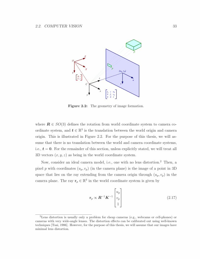
2.2. COMPUTER VISION 33
Figure 2.2: The geometry of image formation.
where R ∈ SO(3) defines the rotation from world coordinate system to camera co-
ordinate system, and t ∈ R3 is the translation between the world origin and camera
origin. This is illustrated in Figure 2.2. For the purpose of this thesis, we will as-
sume that there is no translation between the world and camera coordinate systems,
i.e., t = 0. For the remainder of this section, unless explicitly stated, we will treat all
3D vectors (x, y, z) as being in the world coordinate system.
Now, consider an ideal camera model, i.e., one with no lens distortion.2 Then, a
pixel p with coordinates (up, vp) (in the camera plane) is the image of a point in 3D
space that lies on the ray extending from the camera origin through (up, vp) in the
camera plane. The ray rp ∈ R3 in the world coordinate system is given by
rp ∝ R−1K−1
up
vp
1
(2.17)
2Lens distortion is usually only a problem for cheap cameras (e.g., webcams or cell-phones) orcameras with very wide-angle lenses. The distortion effects can be calibrated out using well-knowntechniques [Tsai, 1986]. However, for the purpose of this thesis, we will assume that our images haveminimal lens distortion.

34 CHAPTER 2. BACKGROUND
where K ∈ R3×3 is the camera matrix [Ma et al., 2005], which projects 3D points
onto the camera plane (see Figure 2.2). Unless otherwise specified, we will assume
that rp has been normalized (i.e., ‖rp‖2 = 1). Note, that any point that lies along
this ray will be projected onto the same image pixel and the pixel’s color or intensity
value will depend on the closest such point. For an ideal camera, the camera matrix
has the form
K =
fu γ u0
0 fv v0
0 0 1
(2.18)
where fu and fv are the (u- and v-scaled) focal lengths3 of the camera, and the
principal point (u0, v0) is the center pixel in the image. The parameter γ models
skewness between the x- and y-imaging axes and can be considered zero for most
practical purposes.
In this thesis, we will generally assume that the image was take with the camera’s
horizontal (x) axis parallel to the ground, and thus only model rotations about this
axis. A tile angle of θ then yields the rotation matrix
R =
1 0 0
0 cos θ sin θ
0 − sin θ cos θ
. (2.19)
Since pixels are discretized, and the recording of light intensity involves noisy
physical processes, the actual generation of an image of a real-world scene is signif-
icantly more complicated than described here. Nevertheless, the description above
provides us with a sufficiently accurate model for 3D reconstruction (as we shall see
in Chapter 6).
3The focal length can be understood geometrically as the distance between the camera centerand the imaging plane.

2.2. COMPUTER VISION 35
Figure 2.3: Convolution of an image with a filter. The value of an output pixel isdetermined by placing the filter kernel over the input image at the corresponding pixellocation. The value is then the dot-product between the reflected filter kernel and the inputimage.
2.2.2 Low Level Image Features
Representing an image by an array of three color components is useful for viewing
and for storage, but not very helpful for automatic scene understanding. For that
we need to extract image features that represent more salient features, such as edges
and textures. One of the first steps towards this higher-level representation is to
convolve the image with a number of different filters. These filters can be applied to
the image’s color channels or, more commonly, to a grayscale version of the image.
Convolution of an arbitrary size input image Ii with a (2w+ 1)× (2h+ 1) kernel
filter K to produce an output (response) image Io, denoted Io = Ii ∗K, is given by
Io(u, v) =w∑
i=−w
h∑
j=−h
Ii(u− i, v − j)K(i, j) (2.20)
This operation is depicted graphically in Figure 2.3. There are several strategies
for dealing with positions where the filter kernel extends beyond the boundary of
the image, including truncating the output image, zero-padding the input image, or
36 CHAPTER 2. BACKGROUND
replicating boundary pixel values. In our work, we adopt the latter approach.
One of the most simple filters is aimed at finding edges in an image by computing
discrete derivatives. The filter is often combined with a Gaussian smoothing filter to
reduce noise. The resulting Sobel filter (for computing vertical gradients) is
K =
−1 0 1
−2 0 2
−1 0 1
=
1
2
1
[
−1 0 1]
(2.21)
which, as can be seen, separates into a vertical smoothing filter and horizontal dif-
ference operator. Horizontal edges can be found by filtering with KT . The gradient
magnitude (or strength) is√I2
x + I2y where Iy and Ix are the vertically and horizon-
tally filtered images, respectively. Similarly, the orientation of the gradient at each
pixel is tan−1(Ix(u, v)/Iy(u, v)). Naively, thresholding the gradient magnitude is a
simple way to find edges but is likely to produce noisy results. Usually, to find better
edges, these Sobel operators are used as a preprocessing stage for a more sophisticated
algorithm, for example, the famous Canny edge detector [Canny, 1986].
Edges and small edge fragments are important features for finding region bound-
aries and identifying objects. However, committing to hard edges as a preprocessing
step often leads to poor performance. A better approach is to robustly describe the lo-
cal edge gradients around each pixel (or a sparse subset of pixels known as keypoints).
One of the most popular methods for describing such local gradient information is the
SIFT descriptor of Lowe [2004]. Briefly, the descriptor is constructed by considering
gradients in a neighborhood region around each pixel. The neighborhood is divided
into a 4× 4 array and each cell further subdivided into a 4× 4 subarray. Smoothed
gradient magnitudes for each cell in the subarrays are accumulated into a histogram
consisting of eight bins according to gradient orientation. These histograms are then
combined (by weighted-average) into histograms for the coarser 4×4 array cells. The
descriptor is rotated by the dominant orientation within the local neighborhood to
provide rotation invariance. The resulting descriptor contains 128 elements (16 his-
tograms, one for each coarse cell, and each histogram containing eight bins). Finally,
the descriptor is normalized to unit length to make it robust to affine changes to

2.2. COMPUTER VISION 37
Figure 2.4: The SIFT feature descriptor. For illustration, the figure shows a 2 × 2descriptor computed from an 8×8 subarray. The standard descriptor, however, is based ona 4× 4 array computed from a 16× 16 subarray. Image courtesy of Lowe [2004].
illumination. An illustration of the SIFT feature descriptor is shown in Figure 2.4.
Filter Banks
Other than the SIFT descriptor (and variants of it), another method for constructing
a better pixel-level image representation is to run a host of different filters over the
image. Per pixel image feature vectors are then constructed by assembling the re-
sponses from this filter bank. A very popular filter bank for multi-class pixel labeling
defines a set of seventeen filters [Shotton et al., 2006]. We will refer to this filter bank
as the texton filter bank. The filter bank is parameterized by a base scale κ.
The first three filters are Gaussian smoothing filters at scales κ, 2κ, and 4κ that
operate on each of the three image color channels. Instead of RGB, the image is first
converted to the more visually perceptive CIELab color space. The Gaussian filter
at scale σ is defined as
G(u, v) =1
2πσ2exp
(
−u2 + v2
2σ2
)
(2.22)
The remaining filters all operate on a grayscale version of the image. The next
four filters are x- and y-derivative-of-Gaussian (DoG) filters at scales 2κ and 4κ. The

38 CHAPTER 2. BACKGROUND
Figure 2.5: Illustration of the 17-dimensional “texton” filters used in multi-class imagesegmentation [Shotton et al., 2006]. Note that the filters operate in CIELab color space(RGB for the color components shown for illustrative purposes only).
x-derivative-of-Gaussian filter is defined by
Gx(u, v) =∂
∂uG(u, v) (2.23)
= − u
σ2r2G(u, v) (2.24)
where r2 = u2+v2
2σ2 . A similar equation exists for the y-derivative, Gy(u, v).
The last four filters are Laplacian-of-Gaussian (LoG) filters at scales κ, 2κ, 4κ,
and 8κ, defined by
LoG(u, v) = ∇2G(u, v) (2.25)
=1
πσ4(r2 − 1) exp(−r2) (2.26)
where ∇2 =(
∂2
∂x2 + ∂2
∂y2
)
is the Laplacian operator and r2 = u2+v2
2σ2 .
An illustration of the seventeen texton filters is shown in Figure 2.5. Response
images when applied to an example input image are shown in Figure 2.6. We use
these filters when building up region appearance features in our scene decomposition
model.
2.2.3 Sliding-Window Object Detection
Sliding-window object detection is a simple yet effective technique for simultaneous
localization and recognition of objects in images. The approach was popularized by
the highly successful work of Viola and Jones [2001, 2004], which aims to find faces
in images in real-time. Some forerunners to the Viola-Jones work also suggested the
sliding-window idea, e.g., [Papageorgiou et al., 1998], and it is now the dominant

2.2. COMPUTER VISION 39
Figure 2.6: Application of 17-dimensional “texton” filters to an image. The originalimage is shown in the top-left corner.
technique for object detection.
The approach involves scanning the image with a fixed-size rectangular window
and applying a classifier to the sub-image defined by the window. The classifier
extracts image features from within the window (sub-image) and returns the proba-
bility that the window tightly bounds an instance from a particular object category.
The process is repeated on successively scaled copies of the image so that objects
can be detected at any size. Figure 2.7 depicts this process. The (x, y)-location of
the window and scale σ of the image implicitly defines the bounding box, or set of
pixels, belonging to the candidate object B(x, y, σ) = (u, v) ⊆ I. Usually a post-
processing set of non-maximal neighborhood suppression is applied to the output set
of bounding boxes to remove overlapping detections of the same object.
Object detection is a very active area of research with new features, improved
classifier technologies, and better learning techniques being developed regularly. In
this thesis we build on two proven sliding-window detectors that vary in the features
and classification engine that they use.

40 CHAPTER 2. BACKGROUND
Figure 2.7: Sliding-window object detection. The image is scanned using a fixed-sizerectangular window and a classifier applied to the sub-image defined by the window at eachlocation. Scanning is repeated on successively down-sampled copies of the image so thatobjects can be detected at different scales.

2.2. COMPUTER VISION 41
Figure 2.8: Feature construction for HOG-based object detector. Image courtesy of Dalaland Triggs [2005].
Histogram of Oriented Gradients Detector
The histogram of oriented gradients (HOG) object detector of Dalal and Triggs [2005]
constructs features motivated by the SIFT descriptor of [Lowe, 2004]. Briefly, x- and
y-derivative filters are applied to the image window, and the orientation of the filter
responses quantized into discrete bins. A histogram over (quantized) orientations
is then constructed in overlapping cells on the detection window by summing the
gradient magnitudes within the cell. Finally, the feature vector is normalized, as was
done for the SIFT descriptor, to make it invariant to affine changes in illumination.
An illustration of the HOG feature construction is shown in Figure 2.8.
The detector learns a separate linear SVM classifier for each object category from
a training set of positive and negative examples (for that category). Robust per-
formance is achieved by running the learned detector over a set of training images
known to not contain the target object category. This produces a set of false positive
examples that are used in a subsequent training iteration to improve the detectors
performance. This step can be repeated, but usually produces very good results after
just one iteration. We incorporate the same strategy to mine for difficult negative
examples when we learn our region-based models.
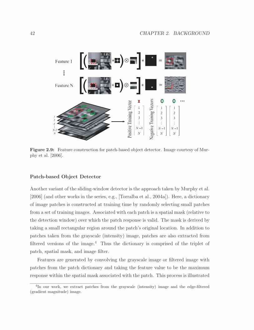
42 CHAPTER 2. BACKGROUND
Figure 2.9: Feature construction for patch-based object detector. Image courtesy of Mur-phy et al. [2006].
Patch-based Object Detector
Another variant of the sliding-window detector is the approach taken by Murphy et al.
[2006] (and other works in the series, e.g., [Torralba et al., 2004a]). Here, a dictionary
of image patches is constructed at training time by randomly selecting small patches
from a set of training images. Associated with each patch is a spatial mask (relative to
the detection window) over which the patch response is valid. The mask is derived by
taking a small rectangular region around the patch’s original location. In addition to
patches taken from the grayscale (intensity) image, patches are also extracted from
filtered versions of the image.4 Thus the dictionary is comprised of the triplet of
patch, spatial mask, and image filter.
Features are generated by convolving the grayscale image or filtered image with
patches from the patch dictionary and taking the feature value to be the maximum
response within the spatial mask associated with the patch. This process is illustrated
4In our work, we extract patches from the grayscale (intensity) image and the edge-filtered(gradient magnitude) image.

2.2. COMPUTER VISION 43
in Figure 2.9. Concretely, the feature value corresponding to the i-th patch is
fi = max(u,v)∈wi
|(Iσ ∗Ki)⊗ gi| (u, v) (2.27)
where Iσ is the image at scale σ, Ki is the filter kernel associated with the i-th patch,
gi is the image patch, wi is the spatial mask, and ⊗ is the normalized cross-correlation
operator.
Given the dictionary of patch features and a set of positive and negative training
images, the approach learns a gentle-boost classifier [Friedman et al., 1998] over two-
split decision stumps for each object category. The patch dictionary is constructed
by randomly selecting patches from the positive training examples. In our implemen-
tation, the patches vary in size from 4 × 4 pixels to half the image window, and we
fix the spatial mask wi to 7 × 7. We then train the object detectors in two stages
for improved efficiency: first we select all positive training examples and a subsample
of negative training examples at random, and train a boosted classifier for a fixed
number of rounds; next, we trim the patch dictionary to remove all patches not used
by this initial classifier; and finally, we retrain using all negative training examples to
obtain the final object detector. Like the HOG-based detector, the process is repeated
on negative examples mined by running the detector over a set of image known not
to contain the object of interest.
Evaluating Object Detector Performance
As discussed, the vast majority of object detection algorithms output bounding boxes
for candidate objects in the image. Associated with each bounding box is an ob-
ject class label and score (e.g., probability). Thus, the output of a (bounding box
based) object detection algorithm is a set of 3-tuples 〈Bi, Ci, si〉 where Bi denotes
the bounding box for the object candidate, Ci denotes its class label, and si denotes
its score. The quality of the object detection algorithm is evaluated by comparing
the detected objects with ground-truth object annotations on a hold-out (unseen
test) set of images. Of interest are the recall of the algorithm—measured as per-
centage of ground-truth objects detected by the algorithm—and the precision of the

44 CHAPTER 2. BACKGROUND
(a) Precision-recall curve (b) Area-of-overlap score
Figure 2.10: Measuring object detection performance. (a) shows a precision-recall curvein red. Performance is summarized by the average precision measured as the 11-pointinterpolated area under the curve. (b) shows calculation of the area-of-overlap score fordetermining correspondence between a ground truth objects Bg and a candidate detectionBd.
algorithm—measured as percentage of detections that are true objects.
The first step in evaluating performance is to decide on a threshold at which to
start considering candidate detections. In general, there will be a trade-off between
precision and recall: The more candidate detections we allow, the greater the chance
that we will detect all the objects in our dataset. However, for a good detector,
the higher we set the detection threshold (i.e., fewer detections), the greater the
chance that we will not see any false-positive detections. This trade-off is captured
by the precision-recall (PR) curve which plots precision against recall as we sweep
over detection thresholds.
The area under the PR curve provides a convenient measure of object detector
performance. It is common to smooth the curve by taking the 11-point average
precision defined by
AP =1
11
10∑
i=0
maxt
p(t) : r(t) ≥ i
10
(2.28)
where p(t) and r(t) are the precision and recall, respectively, at threshold t. Note
that there are a number of other metrics that can be used to measure object detector

2.2. COMPUTER VISION 45
quality, including maximum F1-score, recall at a fixed number of false detections per
image, etc. However, these will not be considered in this thesis.
We are now left with one final problem: How do we determine if a detection
returned by the algorithm corresponds to a ground-truth object? In general, detec-
tion windows will not perfectly align with ground-truth annotations, and so a mea-
sure of overlap is used to determine correspondence. Specifically, the area-of-overlap
score (also known as Jaccard coefficient or intersection-over-union score) measures the
amount of overlap between a detection candidate and a ground-truth object (with the
same class label) by dividing the area of their intersection by the area of their union,
i.e.,
AO(Bd,Bg) =|Bd ∩ Bg||Bd ∪ Bg|
(2.29)
where Bd is the set of pixels belonging to the candidate detection and Bg is the set of
pixels belonging to the ground-truth annotation. A threshold (typically, 0.5 or 0.2)
is then used to decide whether the detection corresponds to the ground-truth object
or not. Note that this notion of overlap can be extended beyond the bounding box
representation to arbitrary pixel sets.
A complication arises when multiple overlapping detections (or ground-truth ob-
jects) are present. In this case, we need to decide which of the overlapping objects
should correspond since each ground-truth object should be explained by at most
one detection. There are two common strategies used to solve this problem. The
first strategy is a greedy approach in which we first sort the candidate detections in
decreasing score and associate ground-truth objects to the overlapping detection with
the highest score.5 The second approach is to form a bipartite graph between the
detection candidates and ground-truth objects where an edge is placed if the area-
of-overlap exceeds some predefined threshold. Edges are weighted by detection score
and correspondences are then determined by finding the maximum matching.
In summary, for evaluation of object detection performance, detection candidates
5If a detection candidate has the choice between two ground-truth objects, it should take the onewith highest overlap score.

46 CHAPTER 2. BACKGROUND
and ground-truth objects are matched using three basic criteria:
• the detection label Ci must match the ground-truth label;
• the detection must have sufficient overlap with the ground-truth object; and
• at most one detection can be associated with a ground-truth object (that is, we
cannot count true-positives multiple times).
With the detection candidates and ground-truth objects matched we can compute
precision and recall values at various thresholds to produce a PR curve and calculate
average precision.
2.2.4 Image Segmentation
Image segmentation can be generally described as the task of partitioning or segment-
ing an entire image into distinct regions. In this section, we review three common
flavors of image segmentation.
Unsupervised Image Segmentation
Unsupervised image segmentation is a bottom-up procedure that aims to group pixels
into regions with similar appearance. The coarseness of the segmentation is deter-
mined by how similar we require the regions to be and can usually be controlled by
a parameter in the algorithm.
Figure 2.11 shows the output of three popular unsupervised segmentation algo-
rithms. The first algorithm, is a graph-based segmentation algorithm by Felzenszwalb
and Huttenlocher [2004]. Briefly, this algorithm creates a graph where the nodes are
pixels and edges connect nodes that are adjacent in the image (i.e., neighboring
pixels). Each edge is weighted by the Euclidean distance between the pixels’ color
vectors. We denote the weight for the edge between pixels p and q by wpq, where
wpq = ∞ if p and q are not adjacent. The algorithm begins by assigning each pixel
to its own region. It then greedily merges regions by considering the weight of edges

2.2. COMPUTER VISION 47
(a) Image (b) Graph-based (c) Mean-shift (d) N-cuts
Figure 2.11: Comparison of different unsupervised image segmentation algorithms. Typ-ical results from (b) the graph-based approach of Felzenszwalb and Huttenlocher [2004], (c)mean-shift segmentation algorithm of Comaniciu and Meer [2002], and (d) normalized-cutsmethod of Shi and Malik [2000]. In terms of runtime, (b) is the fastest and (d) is theslowest.
that span the regions. Specifically, the merge criterion for two regions Pi and Pj is
minp∈Pi,q∈Pj
wpq ≤ min
maxe∈E(mst(Pi))
we + τ(Pi), maxe∈E(mst(Pj))
we + τ(Pj)
(2.30)
where τ(P) = k|P|
is a thresholding function that rewards larger clusters (which may
have better estimates of their appearance), and mst (P) is the minimum spanning
tree over nodes in P . The algorithm is fast, only having to iterate once through all
the edges. However, it can produce irregularly shaped segments, sometimes with long
long tails (i.e., singly connected trails of pixels).
Another popular unsupervised segmentation algorithm is the mean-shift segmen-
tation algorithm of Comaniciu and Meer [2002]. Mean-shift segmentation treats pixels
in an image as 5-dimensional feature vectors (over color and location), and the aim
is estimate the modes of the distribution from which these the vectors (in a given
image) are drawn. This relies on a technique known as kernel density estimation,
which defines the distribution as
f(x) =1
Nhd
N∑
i=1
K
(x− x(i)
h
)
(2.31)
where x(i) are the feature vectors, K(ξ) is a kernel function, d is the dimensionality of
the feature space (i.e., d = 5 for mean-shift image segmentation), and the parameter

48 CHAPTER 2. BACKGROUND
Algorithm 2.5: Mean-shift Segmentation [Comaniciu and Meer, 2002].
Input : xp : p ∈ I // 5-dimensional pixel features1
(hs, hr) // spatial and color range bandwidths2
Output: Pr // segmented image (set of regions)3
foreach pixel p ∈ I do4
set zp = xp5
repeat6
update zp ←P
q∈IK′(zp−xq)xq
P
q∈IK′(zp−xq)
where K(ξ) is defined by Eq. 2.327
until convergence8
end foreach9
group all pixels with zp within neighborhood defined by spatial and range10
bandwidths (hs, hr) into a single region Preturn set of regions Pr11
h ∈ R+ controls the bandwidth of the kernel. For image segmentation the kernel
function is defined as
K(ξ) =C
h2sh
3r
exp
(
−1
2
∥∥∥∥
ξshs
∥∥∥∥
2)
exp
(
−1
2
∥∥∥∥
ξrhr
∥∥∥∥
2)
(2.32)
where hs and hr define the spatial and color range bandwidths, respectively.
The mean-shift algorithm is an iterative algorithm that, beginning at each pixel,
moves to the centroid of the pixels within its neighborhood (defined by the kernel
function). The algorithm iterates until it reaches a stationary point, i.e., a mode.
Segmentation is achieved by grouping all pixels that converge to the same stationary
point. The algorithm is summarized in Algorithm 2.5.
The final unsupervised image segmentation algorithm shown in Figure 2.11 is the
normalized-cuts algorithm. This approach defines a segmentation as a k-way cut
on a graph. Like the the graph-based approach of Felzenszwalb and Huttenlocher
[2004], normalized-cuts defines a graph over pixels in the image. However, here the
edge weights are defined by similarity (i.e., higher is more similar). The cost of any
segmentation is a function of the weights for all edges that are cut (i.e., whose adjacent

2.2. COMPUTER VISION 49
nodes belong to different segments). The key to the algorithm is the method by which
cuts are scored. A naive approach to scoring cuts simply sums over the weights of
the edges that are cut. However, this leads to pathological cases where a single
pixel is segmented from the rest of the image. The crucial insight in normalized-
cuts, is that scoring should take into account the size of the segments that are being
separated. We will skip the details of the actual algorithm, suffice to say that finding
the exact solution defined by the normalized-cuts objective is NP-complete and an
approximate solution is obtained by solving a generalized eigenvalue problem. This
makes the segmentation algorithm very expensive in both storage requirements and
running time.
Most unsupervised segmentation techniques, including all those discussed above,
incorporate a post-processing step that removes small regions by merging them with
adjacent regions.
In our work, we make use of unsupervised image segmentation algorithms to
generate multiple over-segmentations of an image. That is, segmentations in which
the regions are, hopefully, subregions of semantically coherent parts of the image. In
this case, the segments are often called superpixels. The multiple over-segmentations
are generated by varying the parameters (e.g., spatial and color range bandwidths)
of the segmentation algorithms.
Figure/Ground Segmentation
Sometimes we are just interested in segmenting a foreground object (figure) from the
rest of the image. This may be the case when a user provides some indication of which
areas are foreground and which are background, as in the case of interactive segmenta-
tion [Boykov and Jolly, 2001, Rother et al., 2004], or when an instance of a particular
object category is known to be within the image (and well-framed) [Kumar et al.,
2005, Borenstein and Ullman, 2002]. These works typically build appearance models
of the foreground object and surrounding background, and then perform a binary
graph-cut to separate foreground from background along high-contrast boundaries.
In this thesis, we are interested in scenes that contain multiple regions and objects
that we would like to segment, so we do not consider these methods further.

50 CHAPTER 2. BACKGROUND
Multi-Class Image Labeling
Unlike object recognition methods that aim to find a particular object, multi-class
image labeling methods are aimed at concurrent classification of all pixels in an image.
The pixels are classified into one of a predetermined set of labels, e.g., sky, grass, road,
etc., and the segmentation defined by the boundaries between regions having different
semantic labels.
Most multi-class labeling methods achieve their goal by taking into account lo-
cal (pixel or superpixel) appearance signals along with a preference for smoothness,
i.e., classifying visually-contiguous regions consistently. For multi-class image label-
ing, this is often achieved by constructing a conditional Markov random field (CRF)
over the image that encodes local and pairwise probabilistic preferences (e.g., [He
et al., 2004, Shotton et al., 2006]). For example, given a graph G = (V, E) defined
over the image, with nodes V representing pixels or regions and edges E encoding the
neighborhood structure, the CRF is defined as
E(Y ;X) =∑
i∈V
ψi(Yi;X) +∑
(i,j)∈E
ψij(Yi, Yj ;X) (2.33)
where X are features computed from the image (for example, texton filter responses).
An example CRF defined over superpixel regions is illustrated in Figure 2.12. Op-
timizing this energy function is then equivalent to finding the most probable image
labeling.
Performance of multi-class image labeling algorithms is often evaluated by mea-
suring per-pixel accuracy over a hold-out (test) data set. Results can either be micro-
averaged (favoring the larger classes) or macro-averaged (treating all classes with
equal weight). Specifically, for a K-class problem, with predicted labels yiNi=1 and
corresponding ground truth labels yiNi=1, these averages are computed as
Amicro =
∑N
i=1 1yi = yiN
(2.34)
Amacro =1
K
K∑
k=1
∑N
i=1 1(yi = yi) ∧ (yi = k)∑N
i=1 1yi = k(2.35)

2.3. CHAPTER SUMMARY 51
Figure 2.12: Illustration of a conditional Markov random field for multi-class imagelabeling. Highlighted is one of the random variables Yi and one of its neighbors Yj .
where 1P is one if P is true and zero otherwise. In our work, we use the micro-
averaged accuracies when reporting performance.
Like object detection, multi-class image labeling is a very active area of research
with improved techniques being published all the time. The majority of successful
techniques build on the ideas discussed above.
2.3 Chapter Summary
This chapter reviewed some important background material in machine learning and
computer vision. We make use of this material when developing and evaluating our
scene understanding algorithms in subsequent chapters of the thesis.

52 CHAPTER 2. BACKGROUND

Chapter 3
Image Datasets and Dataset
Construction
There have been three significant technological thrusts that have led to the recent
advances in high-level computer vision. First, there has been exponential growth in
raw computational power (both processor speed and system memory) necessary for
running computer vision algorithms. Second, efficient large-scale machine learning
techniques have been developed and low-level feature representations improved (both
of which were previously discussed in Chapter 2) resulting in more robust performance
on novel images. Last, the prevalence of digital cameras and online sharing of media
has resulted in the availability of large quantities of labeled data for training and
evaluation. In this chapter we describe a few of the standard datasets used by the
computer vision community. Our focus will be on datasets applicable to outdoor
scene understanding. We also introduce a new dataset for scene understanding and
describe its construction leveraging Amazon Mechanical Turk (AMT) for labeling.
Unlike previous datasets, this new dataset includes both semantic and geometric
annotations.
53

54 CHAPTER 3. IMAGE DATASETS AND DATASET CONSTRUCTION
3.1 Standard Image Datasets
Image datasets vary across many dimensions according to the purpose for which they
were originally designed. Annotations can vary from global image descriptions to
pixel-level details. For example, a global image description may include the scene
category (e.g., urban, rural, highway, coastal, etc.) or location (e.g., bedroom, bath-
room, kitchen, etc.). At the pixel-level, annotations may include detailed object
outlines or masks.
Datasets intended for object recognition and object detection usually provide
cropped images of objects, where each image is tagged with specific object cate-
gories. These datasets range from relatively small collections with only a few images
per object category, such as the popular Caltech-101 [Fei-Fei et al., 2004] or Caltech-
256 [Griffin et al., 2007] datasets, to “Internet-scale” datasets with millions of images
divided into thousands of object categories, e.g., ImageNet [Deng et al., 2009]. More
sophisticated datasets in this class may also provide bounding box annotations of
objects in the context of a larger scene (i.e., uncropped images) or object outlines,
which are provided either as an explicit set of points along the boundary or as a
segmentation mask. Ponce et al. [2006] give a detailed discussion of the issues in-
volved in constructing datasets for object detection. The authors highlight some
of the problems and artifacts present in the early datasets (e.g., Caltech-101 and
Caltech-256 [Fei-Fei et al., 2004, Griffin et al., 2007]) such as inadequate intra-class
variation (e.g., object pose). These issues are less prevalent in more recent datasets
(e.g., LabelMe [Russell et al., 2008] and PASCAL [Everingham et al., 2010]).
Unlike datasets for object detection, all segmentation and multi-class image la-
beling datasets provide annotations at the pixel level. The Berkeley Segmentation
Dataset [Martin et al., 2001] contains 300 images segmented by multiple human sub-
jects and is intended to provide a basis for developing segmentation and boundary
detection algorithms. The annotations provide information on region boundaries,
but do not provide any semantic information about the regions themselves. Other
datasets, intended for multi-class image labeling, annotate each pixel with a semantic

3.1. STANDARD IMAGE DATASETS 55
(or geometric) class (e.g., the 21-class MSRC dataset [Criminisi, 2004] and the Geo-
metric Context (GC) dataset [Hoiem et al., 2007a]). However, most of these datasets
do not distinguish between multiple instances of the same object class. For exam-
ple, two adjacent cars in an image will be labeled as a single “car” region. More
sophisticated datasets (such as the PASCAL VOC dataset [Everingham et al., 2010]
discussed later) provide both boundary information to separate instances of the same
class and semantic annotations.
Datasets also vary widely in quality. LabelMe [Russell et al., 2008] is a freely
available online dataset with user-supplied annotations. The dataset provides tools
for adding image sets and updating annotations. Little quality control is enforced,
however, resulting in a number of problems including inconsistent names for the same
object, poorly annotated object boundaries, and sparsely labeled images (e.g., only
one object outlined). Researchers typically select a subset of the images from the
LabelMe collection by applying ad hoc filtering rules.
At the other end of the spectrum, the Lotus Hill Research Institute (LHI) has
constructed a commercially available dataset [Yao et al., 2007] for image parsing.
The dataset contains over 600,000 images, which are labeled with accurate region
boundaries and annotated in a part-based hierarchy (e.g., entire cars are segmented
from the rest of the scene, and then each car is further segmented into individual
parts, such as wheels and doors). A subset of the dataset has recently been made
available to academic researchers at no cost.
Between the two extremes of LabelMe [Russell et al., 2008] and LHI [Yao et al.,
2007], the PASCAL Network of Excellence has released a well-annotated dataset as
part of an annual challenge aimed at advancing the state-of-the-art in object detection
techniques. The PASCAL Visual Object Classes (VOC) challenge [Everingham et al.,
2010], initiated in 2005, is run on a dataset of over 7,000 images of realistic scenes.
The dataset is split into training, validation and test, with the training and validation
annotations provided as part of the dataset. Annotations for the test images are
withheld by the organizers so that evaluation must be done by submitting algorithm
results to an online evaluation server. This prevents researchers from inadvertently
over-fitting their models to the test data.
56 CHAPTER 3. IMAGE DATASETS AND DATASET CONSTRUCTION
The PASCAL VOC dataset provides bounding box annotations for 20 object cat-
egories. A subset of the data is also annotated with pixel-level masks for the same
20 object categories. It is becoming the de facto standard for developing and testing
computer vision algorithms. Unfortunately, since the challenge is aimed at object
detection, many of the images (e.g., close-up shots or indoor scenes) and object cate-
gories (e.g., sofas, chairs, computer monitors) are not applicable to the work presented
in this thesis. Furthermore, the dataset does not provide geometric annotations.
To our knowledge, none of the publicly available datasets in the computer vision
community provide both semantic and geometric annotations on the same set of
images. This is problematic for models such as ours, which attempt to exploit the
interaction between semantic classes and scene structure (i.e., geometry). Thus, we
constructed our own dataset, the “Stanford Background Dataset”, formed by taking
images from existing standard datasets and annotating them with suitable semantic
and geometry information. Annotation was performed using Amazon Mechanical
Turk (AMT)—an online marketplace for simple inexpensive jobs. We describe this
dataset and the AMT labeling procedure in Section 3.2. In order to compare to
previously published results we also evaluate our methods on other existing datasets
where appropriate.
The datasets used in this thesis are:
• 21-Class MSRC Segmentation Dataset [Criminisi, 2004]. This dataset
provides pixel-level annotations for 21 different background and foreground ob-
ject categories on 591 images. The labeling is approximate with object bound-
aries tending to be very inaccurate. A further complication is the presence
of many unlabeled pixels (denoted as “void”), which are ignored during both
training and test. Nevertheless, this dataset is a popular dataset for evaluating
the performance of multi-class image labeling algorithms.
• Geometric Context [Hoiem et al., 2007a]. Similar to the multi-class image
labeling datasets for semantic object categories, this dataset provides pixel-level
geometric annotations, e.g., sky, horizontal, vertical, for 300 images of outdoor
scenes. The dataset does not annotate the location of the horizon in the images.
3.1. STANDARD IMAGE DATASETS 57
• Stanford Background Dataset [Gould et al., 2009b]. We constructed this
dataset for the purpose of evaluating the performance of our joint semantic and
geometric scene decomposition model (see Chapter 4). The dataset contains
715 images of urban and rural scenes assembled from a collection of existing
datasets: LabelMe [Russell et al., 2008], 21-class MSRC [Criminisi, 2004], PAS-
CAL VOC [Everingham et al., 2010], and Geometric Context (GC) [Hoiem
et al., 2007a]. The construction of this dataset is the subject of the next sec-
tion. To our knowledge, this is the first dataset to include both semantic and
geometric labels.
• MIT Street Scenes [Bileschi and Wolf, 2005]. This dataset contains a very
large collection of images of Boston street scenes. The images are annotated
with polygonal regions corresponding to a small set of background categories
as well as three foreground objects (cars, pedestrians and bicycles). Labeling is
only approximate and in our experiments we relabeled the background regions
using Amazon Mechanical Turk (see Section 3.2.1).
• CCM (DS1) Dataset [Heitz et al., 2008b]. This dataset is designed for
evaluating holistic scene understanding algorithms and is composed of 422
images of outdoor scenes from various existing datasets (including 21-class
MSRC [Criminisi, 2004], PASCAL VOC [Everingham et al., 2010] and La-
belMe [Russell et al., 2008]). While the source of the images for this dataset
overlaps with the Stanford Background Dataset, very few scenes appear in both
datasets. Each image is annotated with object bounding boxes, pixel semantic
classes, and high-level scene category (e.g., urban, rural, harbor). The dataset
includes six object categories (boat, car, cow, motorbike, person, and sheep) and
the same eight pixel-level semantic classes as the Stanford Background Dataset.
We use this dataset in Chapter 5 to evaluate our object detection performance.
• Make3d [Saxena et al., 2005, 2008]. This dataset is composed of 534
images of outdoor scenes with corresponding depth maps. The depth maps
were collected using a laser range finder with maximum range of 81 meters. One
of the limitations of this dataset is the lack of foreground objects due to the
58 CHAPTER 3. IMAGE DATASETS AND DATASET CONSTRUCTION
relatively long time required for the laser range finder to scan the scene during
data capture. We use this dataset in Chapter 6 for training and evaluating our
semantically-informed depth perception algorithms.
3.2 Stanford Background Dataset
The Stanford Background Dataset is a new dataset introduced as part of this work
for evaluating methods for geometric and semantic scene understanding. The dataset
contains 715 images chosen from existing public datasets, namely, LabelMe [Russell
et al., 2008], 21-class MSRC [Criminisi, 2004], PASCAL VOC [Everingham et al.,
2010], and Geometric Context (GC) [Hoiem et al., 2007a]. Our selection criteria were
for the images to be of outdoor scenes, have approximately 320× 240 pixels, contain
at least one foreground object, and have the horizon positioned within the image (it
need not be visible).
Ground truth labels for training and testing were obtained using Amazon Me-
chanical Turk (AMT), as discussed in Section 3.2.1 below. The dataset provides
eight semantic region labels: sky, tree, road, grass, water, building, mountain, and
foreground object ; and three geometric region labels: sky, horizontal (support), and
vertical. In addition, the location of the horizon is also provided. The quality of
our annotations (obtained using AMT) is extremely good and in many cases supe-
rior to those provided by the original datasets where available (see Figure 3.3 for a
comparison with MSRC).
3.2.1 Amazon Mechanical Turk
Amazon Mechanical Turk (AMT) (http://www.mturk.com/) is an online market-
place where requesters can post simple jobs for non-expert workers to complete.
Typical jobs—known as Human Intelligence Tasks (HITs)—involve completing on-
line surveys, giving feedback on website designs, writing textual descriptions or rec-
ommendations for products, transcribing text from audio recordings, etc. Workers
3.2. STANFORD BACKGROUND DATASET 59
are paid between one cent and a few dollars per task.1 Researchers in the machine
learning community have discovered AMT as a cheap source of supervised training
data [Sorokin and Forsyth, 2008, Snow et al., 2008]. For example, construction of
the ImageNet [Deng et al., 2009] dataset which contains over nine million images or-
ganized into a conceptual-semantic hierarchy (i.e., noun hierarchy) was only possible
thanks to the cheap online workforce and infrastructure provided by AMT.
In our work, we used AMT to acquire human-labeled ground truth region bound-
aries, semantic labels and geometric labels for our Stanford Background Dataset (first
introduced in Gould et al. [2009b]), and to relabel some existing datasets such as the
MIT Street Scenes [Bileschi and Wolf, 2005] dataset described above. We developed
an Adobe Flash application which allowed users to “paint” over an image with a color
indicating the category of the underlying pixel (or a unique color for each region in
the image). For example, the users were asked to paint grass as green, water as blue,
and buildings as red. A screenshot of our application is shown in Figure 3.1.
We configured our application for three different tasks per image:
• Region labeling: Here workers were instructed to label each region (i.e., object
or distinct background area) in the image with a different color. Specific exam-
ples were shown of adjacent objects “painted” in different colors. The workers
were asked to pay particular attention to accurate labeling of the boundary
between regions.
• Semantic labeling: In this task, the workers were asked to label each pixel
in the image with the color corresponding to one of eight semantic classes.
Pixels not belonging to one of the classes could be left unlabeled (i.e., white).
However, since our set of semantic classes covered most background regions
found in outdoor scenes, and included a generic foreground object label, the
vast majority of images were densely labeled.
• Geometry labeling: Similar to the semantic labeling task, in this task workers
were asked to label each pixel in the image with a color corresponding to one of
1A rule-of-thumb is for workers to be paid approximately $1.00 per hour of work.

60 CHAPTER 3. IMAGE DATASETS AND DATASET CONSTRUCTION
three course geometric classes. Slanted surfaces were to be assigned the label
(horizontal or vertical) closest to the true orientation.
The tasks were uploaded onto AMT with simple instructions to workers (see Fig-
ure 3.1) and examples of both good and bad quality annotations. Workers were paid
$0.10 per task per image. Thus, for under $250 we were able to label our entire
715-image dataset.2 Typical labels obtained from AMT are shown in Figure 3.2. As
can be seen, the quality of these labels is very good. In particular, when compared
to other datasets, our annotations provide a dense labeling of the image (i.e., every
pixel is assigned a class label) and the region boundaries are very close to the true
object boundaries. Figure 3.3 illustrates this on two example images from the 21-class
MSRC dataset [Criminisi, 2004].
We also developed back-end verification tools which, allowed us to quickly verify
the quality of the labels and approve or reject the work. Approximately 10% of the
jobs were rejected due to poor quality.3 Figure 3.4 shows examples of jobs that were
rejected. In some cases jobs were rejected because of egregious errors (such as the
first row in Figure 3.4), while others were due to the AMT worker misunderstanding
the labeling instructions. In all cases, the rejected images were re-submitted to AMT
and were usually labeled correctly the second time.
The back-end verification process, while streamlined, did require some manual ef-
fort on our part (albeit far less effort than had we chosen to label the images ourselves).
Some researchers have suggested that AMT can also be used in the verification stage
by having a separate set of jobs in which workers rate the quality of each labeling.
By providing known good and bad examples, having trusted workers, or getting the
same image rated multiple times, one could ensure the integrity of this verification
stage, and thus completely automate the labeling process.
Since labeling of the location of the horizon required little effort, for the 715 images
in our dataset, we elected to perform this annotation ourselves. However, this task
can easily be converted into an AMT job for future labeling of larger scale datasets.
2We uploaded our images in batches as we were familiarizing ourselves with the AMT systemand debugging our code. Typically, a batch of 100 images would get labeled overnight (i.e., in under12 hours).
3Rejected jobs do not get paid.

3.3. CHAPTER SUMMARY 61
3.3 Chapter Summary
Labeled training data is necessary for training the machine learning algorithms used
by computer vision researchers, and having standard high-quality datasets is essential
for evaluating and comparing the performance of these algorithms.
In this chapter we have provided a brief description of the standard datasets used
in the computer vision community and, in particular, for evaluating the methods
presented in this thesis. We discussed some of the problems with early datasets that
are slowly being corrected in newer (and larger) datasets. To support some of the
experiments that we wanted to run, we introduced a new dataset containing both
semantic and geometric labels. The labeling of this dataset was performed using
Amazon Mechanical Turk at a total cost of under $250.

62 CHAPTER 3. IMAGE DATASETS AND DATASET CONSTRUCTION
Figure 3.1: Screenshot of an Amazon Mechanical Turk HIT for labeling regions in animage. Our tool can be configured for labeling different tasks including regions (e.g., withmultiple distinct object instances), semantic classes (by pixel), and geometry.

3.3. CHAPTER SUMMARY 63
(a) Image (b) Regions (c) Semantics
Figure 3.2: Typical label quality obtained from AMT jobs. Column (a) shows the imagebeing labeled; column (b) shows the annotated regions (each color represents a uniqueregion); and column (c) shows the pixel semantic classes (see semantic legend).

64 CHAPTER 3. IMAGE DATASETS AND DATASET CONSTRUCTION
(a) Image (b) AMT Labels (c) MSRC Labels
Figure 3.3: Comparison of the label quality obtained from our AMT jobs versus the21-class MSRC [Criminisi, 2004] dataset. White indicates unlabeled (“void”) pixels thatare not considered during training or evaluation. The MRSC “cow” label (second row) hasbeen mapped to “foreground” for comparison with our semantic classes.

3.3. CHAPTER SUMMARY 65
(a) Image (b) Poor Labeling (c) Reworked Labels
Figure 3.4: Two examples of poorly labeled images obtained from a semantic labelingjob on Amazon Mechanical Turk (AMT). The first example (top row) shows correct regionboundaries, but incorrect semantic labels. The second example (bottom row) shows a linedrawing of the image, indicating a misunderstanding of the labeling instructions by theAMT worker. These images were resubmitted to AMT for subsequent annotation. In total,only about 10% of jobs required rework.

66 CHAPTER 3. IMAGE DATASETS AND DATASET CONSTRUCTION

Chapter 4
Scene Decomposition: From Pixels
to Regions
In this chapter, we introduce our scene decomposition model. We begin by describing
the various entities of the scene that we will reason about and formalize them in
terms of random variables in a probabilistic graphical model. We develop the model
up to the stage of scene decomposition, that is, breaking the image into semantic and
geometrically consistent regions, and leave the discussion of specific object identifica-
tion and outlining until Chapter 5. Our aim, therefore, is to be able to decompose a
scene into a number regions that are annotated with a class label from one of many
background class types or single foreground object class that will later (in Chapter 5)
be refined into specific object categories. In addition to annotating the regions with
semantic class labels, we will also assign coarse geometric labels to the regions and
predict the location of the horizon in the image.
This initial scene decomposition is an important step towards the goal of holistic
scene understanding since such an analysis gives a high-level understanding of the
overall structure of the scene, allowing us to derive a notion of relative object scale,
height above ground, and placement relative to dominant semantic categories such as
road, grass, water, buildings or sky. Unlike methods that deal only with multi-class
semantic labeling (e.g., [Shotton et al., 2006]) or only with geometric reconstruction
(e.g., [Hoiem et al., 2007a]), our approach reasons jointly about both aspects of the
67

68 CHAPTER 4. SCENE DECOMPOSITION
Figure 4.1: Example of a typical urban scene demonstrating that most background regionscan be easily recognized from local color and texture cues whereas foreground regions requirecomplex shape and appearance models.
scene, allowing us to avoid inconsistencies (such as vertical roads) and to utilize
contextual relationships to reduce false positive objects (such as those not supported
by a horizontal region).
Our decision to first concentrate on background semantic classes is not accidental.
Consider the various regions present in the typical urban scene shown in Figure 4.1.
Notice how the foreground classes (“things”)—such as cars and trucks—require com-
plex shape and appearance models, while background classes (“stuff”)—such as sky,
road and grass—can often be identified from simple texture and color cues. This ob-
servation is supported by our own experiments and results from many seminal works
in multi-class image labeling. For example, on the 7-class Corel dataset considered by
He et al. [2004] 93.7% of the background pixels are classified correctly compared to
82.1% for foreground. On the challenging 21-class MSRC dataset [Criminisi, 2004],
the difference is even more stark (e.g., 94.5% versus 63.1% for Shotton et al. [2006]
and 90.5% versus 68.3% for Ladicky et al. [2009]).1 Our hope, then, is that relatively
1We computed these performance metrics by grouping the multiple classes considered by eachof the works into background and foreground, and then averaging over the results provided in therespective publications.

69
simple models will allow us to characterize background and separate it from fore-
ground regions, which we can then recognize using more sophisticated methods. As
we will see, this is precisely the effect that results from running our decomposition
model.
A key aspect of our approach is the use of large, dynamically-defined regions as the
basic semantic unit. Most previous methods for doing this type of image decomposi-
tion use either individual pixels [Shotton et al., 2006] or predefined superpixels [Yang
et al., 2007, Gould et al., 2008]. Here, a superpixel is defined to be a connected
set of pixels having similar appearance. Each of these approaches has its trade-offs.
The use of individual pixels makes it difficult to utilize more global cues, including
both robust statistics about the appearance of larger regions, which can help average
out the random variations of individual pixels, and relationships between regions,
which are hard to “transmit” by using local interactions at the pixel level. The use
of superpixels partially addresses some of these concerns, but as superpixels are con-
structed in advance using simple bottom-up procedures based on local appearance,
their boundaries are often inconsistent with the true region boundaries, making an ac-
curate decomposition of the image impossible. Our approach dynamically associates
pixels to regions, allowing region boundaries to adjust so as to accurately capture the
true object boundaries. Moreover, our regions are also much larger than superpixels,
allowing us to derive global appearance properties for each region, including not only
color and texture, but even larger properties such as its general shape, aspect ratio,
and characteristics of its boundary.
Reasoning in our model requires that we infer both the pixel-to-region association
and the semantic and geometric labels for the regions. We address this challenge
using a hybrid inference approach. For the pixel-association task, we propose a novel
multiple-segmentation approach, in which different precomputed over-segmentations
are used to propose changes to the pixel-to-region associations. These proposed moves
take large steps in the energy space and hence help avoid local minima; however, they
are evaluated relative to our global energy function, ensuring that each step reduces
the energy, and hence improves the decomposition of the scene at hand. The region-
labeling task is addressed using global energy-minimization methods over the region

70 CHAPTER 4. SCENE DECOMPOSITION
space (conditioned on the current pixel-to-region assignments). This step is not too
expensive, since the number of regions is significantly lower than the number of pixels.
By performing the inference at this level, we also improve labeling accuracy because
the adjacency structure between these larger regions allows us to directly exploit
correlations between them (such as the fact that ground is below sky).
The parameters of our model are entirely learned from data. Recall that in our
model, we are learning to label entire segments, allowing us to exploit global region-
level characteristics. We obtain positive examples for region labels from a large train-
ing set, which we constructed using Amazon Mechanical Turk (AMT) as discussed
in Chapter 3. Negative examples are a bit trickier to acquire, as there are exponen-
tially many “non-regions,” most of which are obviously bad choices. Training with all
non-regions is clearly intractable, and training with a random subset would be mis-
leadingly easy for the learning algorithm. We therefore propose a novel closed-loop
training regime, where the algorithm runs inference on the training images given its
current model parameters, and mines for mistakes. These mistakes are then used as
negative examples for a subsequent parameter learning iteration. This focuses the
learning process on improving cases that are likely to occur in practice.
We now turn to describing the various entities in our model. Inference and learning
are described in Section 4.2.1 and Section 4.2.2, respectively. In Section 4.3 we apply
our method to the challenging Stanford Background Dataset (see Chapter 3) and show
that our approach produces multi-class segmentation and surface orientation results
that outperform state-of-the-art methods. We conclude the chapter in Section 4.4
with a summary of our model and discussion of the conclusions that can be drawn
from this work.
4.1 Scene Decomposition Model
Our goal is to decompose an image I into an unknown number (K) of geometrically
and semantically consistent regions by iteratively optimizing an energy function that
measures the quality of the solution at hand. Our model reasons about both pixels
and regions. Each pixel in the image p ∈ I belongs to exactly one region, which
4.1. SCENE DECOMPOSITION MODEL 71
is identified by the pixel’s region-association variable Rp ∈ 1, . . . ,K. Let the set
of pixels in region r be denoted by Pr = p : Rp = r. The size of the region
(i.e., number of pixels) is simply Nr = |Pr| =∑
p 1Rp = r. In our notation we
will always use subscripts p and q to denote pixels, and subscripts r and s to denote
regions. Double indices are used for pairwise terms between adjacent entities in the
scene (e.g., pq or rs).
Each pixel has a local appearance feature vector αp ∈ Rn (described in Sec-
tion 4.1.2 below). Associated with each region are: a semantic class label Sr, cur-
rently grass, mountain, water, sky, road, tree, building and foreground; a geometric
class label Gr, currently horizontal, vertical, and sky; and a region appearance Ar
that summarizes the appearance of the region as a whole.
The final component in our model is the horizon. We assume that the image was
taken by a camera with horizontal axis parallel to the ground. We therefore model
the location of the horizon as the row in the image corresponding to the horizon
vhz ∈ 1, . . . , height(I).Given an image I and model parameters θ, our unified energy function scores the
entire description of the scene: the pixel-to-region associations R; the region semantic
class labels S, geometries G, and appearances A; and the location of the horizon vhz:
E(R,S,G,A, vhz | I,θ) = ψhorizon(vhz) +∑
r
ψregionr (Sr, Gr, v
hz;Ar,Pr)
+∑
r,s
ψpairrs (Sr, Gr, Ss, Gs;Ar,Pr, As,Ps) +
∑
p,q
ψboundarypq (Rp, Rq;αp, αq). (4.1)
Each of the terms in the energy function captures a preference for assignments to
a subset of the variables in the model. Together they provide a global score for any
given scene decomposition (i.e., complete assignment to all the variables). We now
describe each of these terms.
4.1.1 Predicting Horizon Location
The ψhorizon term in our energy function (Equation 4.1) captures the a priori estimate
of the location of the horizon in the scene. In our model, it is implemented as a
72 CHAPTER 4. SCENE DECOMPOSITION
log-gaussian potential function
ψhorizon(vhz) = −ηhorizon logN (vhz;µ, σ2) (4.2)
with parameters µ and σ learned from labeled training images. Note that the horizon
variable vhz also appears in each of the ψregion terms so that during inference, its
optimal value will be determined by taking into consideration the preference from
both the ψhorizon and ψregion terms. The constant ηhorizon in Equation 4.2 weights the
contribution of this term relative to the other terms in the energy function.
It should be stressed that this term implements a simple prior on the location of
the horizon. A number of techniques have been proposed in the literature [Quan and
Mohr, 1989, Kosecka and Zhang, 2002, Hoiem et al., 2006] that attempt to estimate
the location of the horizon using more sophisticated approaches such as looking for
vanishing lines. We found that a reliable estimate of the horizon could be achieved on
our dataset by our simple log-gaussian prior and the inclusion of the horizon variable
in the region term. Thus, the additional complexity of these more sophisticated
methods was not warranted.
4.1.2 Characterizing Individual Region Appearance
For each pixel p in the image, we construct a local appearance descriptor vector
αp comprised of raw image features and discriminatively learned boosted features.
Our raw image features, which are computed in a small neighborhood of the pixel,
are identical to the 17-dimensional color and texture features described by Shotton
et al. [2006] (see Chapter 2). We augment these raw features with more processed
summaries that represent the “match” between the pixel’s local neighborhood and
each of the region labels. Specifically, for each (individual) semantic and geometric
label we learn a one-vs-all boosted classifier to predict the label given the raw image

4.1. SCENE DECOMPOSITION MODEL 73
Pixel Feature Description
Filter Responses (17) Color and texture filter responses describedin Shotton et al. [2006]
Boosted Classifier Scores (11) Log-odds ratio from one-vs-all boosted clas-sifiers trained to predict individual pixel se-mantic and geometric class labels from thepixel’s appearance and location, and the ap-pearance of pixels in a small neighborhoodaround it.
Table 4.1: Local pixel appearance features, αp.
features in a small neighborhood around the pixel.2 We then append the score (log-
odds ratio) from each boosted classifier to our pixel appearance feature vector αp.
Table 4.1 summarizes these features.
We infer the region appearance Ar by fitting a multi-variate Gaussian over the
appearance of pixels within the r-th region. That is, we set Ar =(µA
r ,ΣAr
)where
µAr ∈ R
n and ΣAr ∈ R
n×n are the maximum-likelihood Gaussian mean and covariance
parameters, respectively:
µAr =
1
Nr
∑
p∈Pr
αp (4.3)
ΣAr =
1
Nr
∑
p∈Pr
(αp − µA
r
) (αp − µA
r
)T(4.4)
These summary statistics give us a more robust estimate of the appearance of the
region than would be obtained by considering only small neighborhoods of the indi-
vidual pixels.
2In our experiments, we append to the pixel’s 17 “texton” features, the average and variance foreach feature over a 5 × 5-pixel window in 9 grid locations around the pixel and the image row togive a total of 324 features. We use the GentleBoost algorithm [Friedman et al., 1998] with 2-splitdecision stumps and train for 500 rounds. Our results appeared robust to the choice of parameters.

74 CHAPTER 4. SCENE DECOMPOSITION
4.1.3 Individual Region Potentials
To define the potentials that help infer the label of individual regions, we extract
features φr(Ar,Pr) ∈ Rn describing the region appearance and basic shape. These
features are summarized in Table 4.2. Our appearance features include the mean
and variance over the appearance of the pixels in the region as described above, and
the log-determinant of the covariance matrix over pixel appearances (i.e., log |ΣAr |) to
capture total variation in pixel appearance. We also include the average contrast at
the region boundary and region interior which gives a sense of the region’s internal
texture versus its surrounding. In addition to relating to semantic class—grass is
green; sky is blue—these appearance features provide a measure for the quality of
a region since well-formed regions will tend to have strong boundary contrast and
(depending on the class) little variation of interior appearance.
We also want to capture more global characteristics of our larger regions. For
example, we would like to capture the fact that buildings tend to be vertical with
many straight lines, trees tend to be green and textured, and grass tends to be green
and horizontal. Thus, we incorporate shape features that include normalized region
area, perimeter length, first- and second-order shape moments, and residual to a
robust line fit along the top and bottom boundary of the region.3 The latter features
capture the fact that buildings tend to have straight boundaries while trees tend to
be rough.
We also include the horizon variable in the region-specific potential, allowing us
to include features that measure the ratio of pixels in the region above and below
the horizon. These features give us a sense of the scale of the object and its global
position in the scene. For example, buildings are tall and tend to have more mass
above the horizon than below it; foreground objects are often close and will have most
3Specifically, let Pr be the set of pixels in the region and let B = (ui, vi) ⊆ Pr be the set
of pixels along its perimeter (boundary). Then the normalized region area is |Pr||I| ; the length of
the perimeter is simply |B|; the first- and second-order shape moments are µx = 1|Pr|
∑
(u,v)∈Pru
and σ2x = 1
|Pr|
∑
(u,v)∈Pr(u − µx)2 and similarly for y, and σ2
xy = 1|Pr|
∑
(u,v)∈Pr(u − µx)(v − µy);
and, finally, the residual along the top and bottom boundary of the region is computed by linearleast-squares regression to the subset of pixels in B that are the topmost and bottommost in theircolumns, respectively.

4.1. SCENE DECOMPOSITION MODEL 75
Region Feature Description
Appearance (57) Mean and standard deviation of the 17-dimensional fil-ter responses and boosted classifier score for each pixelin the region, and log-determinant of the appearancecovariance matrix ΣA
r .
Boundary Contrast (4) Measure of the contrast along the boundary of the regionrelative to its interior. They include the mean pixelwisecontrast along the boundary; the average boundary con-trast divided by the square-root of the region’s area; theaverage internal contrast; and the ratio of boundary con-trast to total (boundary plus internal) contrast.
Shape (19) Basic region shape such as size and extent (relative toimage dimensions), perimeter length, residual to linesfitted along the top and bottom boundary (as a measureof “straightness”), and first- and second-order shapemoments. They also include binary features indicatingwhether the region has been truncated by the edge, top,or bottom of the image.
Geometry (9) These features capture the relative location of the regionwith respect to the horizon vhz and include the percent-age of pixels in the region above and below the horizon;the spread of pixels about the horizon (i.e., mean dis-tance above and below the horizon).
Table 4.2: Summary of the features φr(Ar,Pr) used to describe regions in our model.

76 CHAPTER 4. SCENE DECOMPOSITION
of their mass below the horizon. Conversely, these potentials also allow us to capture
the strong positional correlation between the horizon and semantic classes such as
sky or ground, allowing us to use the same potential to place the horizon within the
image.
To put all of these features together, we learn a multi-class logistic classifier over
the joint assignment to semantic and geometric class labels Sr ×Gr with a quadratic
kernel over φr (see Section 4.2.2). The score for any assignment to the region variables
is then
ψregionr (Sr, Gr, v
hz;Ar,Pr) = −ηregionNr log σ(Sr ×Gr | φr(Ar,Pr), v
hz), (4.5)
where ηregion weights the importance of the region energy term relative to the other
terms in the energy function and σ(·) is the multi-class logistic function with learned
parameters. We scale the potential by the region size Nr so that our score gives more
weight to larger regions and is independent of the number of regions in the image.
4.1.4 Inter-Region Potentials
Our model contains two types of inter-region potentials. The first of these terms is
ψboundarypq , which is a standard contrast-dependent pairwise boundary potential [Shot-
ton et al., 2006]. Concretely, for two adjacent pixels p and q, we define
ψboundarypq (Rp, Rq;αp, αq) =
ηbndry exp−12β−1‖αp − αq‖2, if Rp 6= Rq
0 otherwise(4.6)
where β is an image-specific normalization constant set to the average contrast be-
tween all adjacent pixels in the image. Specifically, we have
β =1
|E|∑
(p,q)∈E
‖αp − αq‖2 (4.7)
where the summation is over all pairs of adjacent pixels in the image denoted by
the set E . In practice, we restrict αp and αq to the first three color components

4.1. SCENE DECOMPOSITION MODEL 77
(i.e., CIELab color coordinates) of the full pixel appearance feature vector. This
term penalizes adjacent regions that do not have an edge between them; it has the
effect of trying to merge adjacent regions that are not clearly demarcated. We note
that, since the penalty is accumulated over pairs of adjacent pixels, the region-level
penalty is proportional to the pixel-length of the boundary between the regions.
Our second inter-region potential, ψpair, models the affinity of two semantic or
geometric classes to appear adjacent to each other (as separate regions). Similar to the
within-region potentials, we extract features φrs(Ar,Pr, As,Ps) ∈ Rm for every pair
of adjacent regions r and s. We then learn independent multi-class logistic classifiers
for Sr × Ss and Gr ×Gs given these features. Note that these pairwise potentials are
asymmetric (e.g., exchanging Sr and Ss gives a different preference since, as we shall
see, the features include orientation information). The features φrs are intended to
capture contextual properties between regions, for example, the boundary between
building and sky tends to be straight and building is more likely to appear above a
foreground object than below it. To capture these properties, our features include
the difference between centroids of the two regions, the proportion of pixels along the
boundary in which region r is above/below region s, the length of the boundary, the
residual after fitting a straight line to the boundary pixels, and the orientation of this
line.4 In addition to these layout-based features, we include appearance difference
between the regions normalized by the total appearance variance within each region.
This captures signals such as foreground objects tend to contrast highly with other
regions, whereas background regions are more similar in appearance, such as adjacent
buildings in a city. The pairwise region features φrs are summarized in Table 4.3.
We normalize each pairwise potential by the sum of the number of pixels in each
region divided by the number of neighbors for the region:(
Nr
|nbr(r)|+ Ns
|nbr(s)|
)
. This
makes the total influence on a region independent of its number of neighbors while
still giving larger regions more weight. The final form of our second inter-region
4As for the region boundary features, the pairwise boundary terms are computed using a linearleast-squares fit to the boundary pixels. Specifically, let B = (ui, vi) be the set of pixels alongthe boundary between regions r and s. Then the length of the boundary is simply the number ofpixels |B|; the residual is computed as minθ
∑
(ui,vi)∈B ‖vi − θ1ui + θ0‖ (i.e., performing a linear
least-squares fit); and the orientation of this line is taken as θ1.

78 CHAPTER 4. SCENE DECOMPOSITION
potential is then
ψpairrs (Sr, Gr, Ss, Gs;Ar,Pr, As,Ps) = −ηpair
(Nr
|nbr(r)|+ Ns
|nbr(s)|
)
·(
log σ (Sr × Ss | φrs) + log σ (Gr ×Gs | φrs))
, (4.8)
where, as above, ηpair weights the pairwise region potential relative to the other terms
in the energy function, and σ(·) is the multi-class logistic function (with quadratic
kernel over the features φrs as was done for the individual region potentials in the
previous section).
Pairwise Feature Description
Centroid (2) Difference between the centroids of regions rand s (in normalized image coordinates).
Relative Position (2) Percentage of pixels along the boundary be-tween regions r and s for which (i) region ris above region s, and (ii) region r is belowregion s.
Boundary (3) Number of pixels along the boundary be-tween regions r and s, the residual after fit-ting a straight line to the boundary pixels,and the orientation of this line.
Appearance (28) The difference between the average appear-ance features of regions r and s normalizedby the standard deviation of the feature,
i.e., diag(σA
r + σAs
)−1(µA
r −µAs ) where σA
r isthe square-root of the diagonal of ΣA
r .
Table 4.3: Summary of the features φrs(Ar,Pr, As,Ps) used to describe the pairwiserelationship between two adjacent regions in our model.

4.2. INFERENCE AND LEARNING 79
4.2 Inference and Learning
4.2.1 Inference Algorithm
Exact inference in our decomposition model is clearly intractable. We therefore adopt
a two-stage hill climbing approach to approximately minimize the energy defined by
Equation 4.1. In the first stage, we modify the pixel-to-region association variables
by allowing a set of pixels to change the region to which they are assigned. Given the
new pixel assignments, we then jointly optimize the region and horizon variables in
the second stage. The global energy of the resulting configuration is then evaluated,
and the move is accepted only if this energy decreases, ensuring that our inference is
continuously improving a coherent global objective.
The proposal moves for region associations are drawn from a precomputed, image-
specific dictionary of image segments Ω, an example of which is shown in Figure 4.2.
We build the segments by computing a number of different over-segmentations of the
image. Here, we use the mean-shift algorithm [Comaniciu and Meer, 2002], but could
equally have used other approaches for generating over-segmentations (e.g., graph-
based clustering [Felzenszwalb and Huttenlocher, 2004] or normalized-cuts [Shi and
Malik, 2000]).5 We generate different over-segmentations by varying the spatial and
range bandwidth parameters and add all generated segments to the dictionary. This
produces a rich set of fine and coarse granularity proposal moves. We sort the moves
in the dictionary by the entropy of pixel appearance within each segment so that more
uniform segments are proposed first. In addition to moves proposed by the dictionary,
we also allow moves in which two adjacent regions are merged together. The set of
allowed pixel-to-region association proposal moves is thus: (i) pick a segment ω ∈ Ω
and assign all Rp for p ∈ ω to a new region; (ii) pick a segment ω ∈ Ω and assign all
Rp for p ∈ ω to one of the regions in its neighborhood; or (iii) pick two neighboring
regions r and s and merge them, that is, ∀Rp = s set Rp = r.
5Publicly available code exists for many of the over-segmentation algorithms. We used an imple-mentation of the mean-shift algorithm that can be downloaded from:http://www.caip.rutgers.edu/riul/research/~code/EDISON/index.html

80 CHAPTER 4. SCENE DECOMPOSITION
Figure 4.2: Example over-segmentation dictionary, Ω, for a given image generated byrunning mean-shift [Comaniciu and Meer, 2002] with three different parameter settings,(hr, hs) ∈ (6, 7), (6, 11), (6, 19). The figure shows the boundary of each segment overlayedon top of the original image. In our inference algorithm, each segment ω ∈ Ω defines a setof pixels-to-region association variables Rp : p ∈ ω that may be re-assigned to anotherregion.
We note that, in our current implementation, we do not allow regions to be discon-
nected, although such situations might occur in practice (for example, a bus whose
middle is occluded by a foreground tree). This is ensured during the proposal move by
reassigning region identifiers if the move results in a disconnected component. Since
checking for connected components has to be done after every proposal move, we have
developed fast techniques for performing this step (see Appendix A.2).
Our overall inference procedure is summarized in Algorithm 4.1. Briefly, we ini-
tialize our pixel-to-region association variables R using one of the over-segmentations
used to produce our dictionary, and greedily infer the remaining variables in the model
(S, G and vhz). We then cycle over proposal moves: Given our current associations
R, we select a proposal move and reassign pixels to form new regions. Next, we
update the appearance model Ar and features of any region that was affected by the
move. We maintain sufficient statistics over pixel appearance, making this step very
fast (see Appendix A.1). Keeping the pixel-to-region association variables and hori-
zon fixed, we run max-product belief propagation on the region class and geometry
variables. We then update the horizon vhz using a greedy minimization step condi-
tioned on the remaining variables.6 The new configuration is evaluated relative to
6We experimented with including vhz in the belief propagation inference but found that it changedvery little from one iteration to the next and was therefore more efficient to infer conditionally oncethe other variables were assigned.

4.2. INFERENCE AND LEARNING 81
Algorithm 4.1: Scene Decomposition Inference.
Input : I // image1
θ // model parameters2
Output: R,S,G, and vhz // scene decomposition3
generate over-segmentation dictionary Ω4
initialize Rp using one of the over-segmentations5
infer initial Sr, Gr and vhz variables6
compute energy of initial assignment and store in Emin7
repeat8
foreach proposal move ω do9
move pixels Rp : p ∈ ω ← r10
update region appearance A and features11
run inference over region variables (S,G) and horizon vhz12
compute total energy E of new assignments13
if (E < Emin) then14
accept move and set Emin = E15
else16
reject move17
end18
end foreach19
until convergence20
return R,S,G, and vhz21
our global energy function, and kept if it provides an improvement. The algorithm
iterates until convergence, i.e., none of the proposal moves result in a lower energy
assignment. In our experiments (Section 4.3) inference took between 30 seconds and
10 minutes to converge depending on image complexity (i.e., number of segments in
the dictionary Ω).
4.2.2 Learning Algorithm
We train our model using a labeled dataset where each image is segmented into regions
that are semantically and geometrically coherent. Thus, our ground truth specifies
both the region association for each pixel, Rp, and the semantic and geometric labels
for each region, Sr and Gr.

82 CHAPTER 4. SCENE DECOMPOSITION
We learn each term ψhorizon, ψregion and ψpair in our energy function separately,
using our labeled training data. Learning is done using a maximum likelihood objec-
tive with small ℓ2-regularization on the parameters (see Chapter 2 for details). We
then cross-validate the weights between the terms to maximize our pixelwise labeling
accuracy on a subset of our training data. Since only the relative weighting between
terms matter, we fixed ηregion to one.
For the horizon singleton term, we learn a Gaussian over the location of the horizon
in training images and set ψhorizon to be the log-likelihood of vhz given this model.
We normalize vhz by the image height to make this model resolution invariant. Our
learned Gaussian has a mean of approximately 0.5 and standard deviation of 0.15
(varying slightly across experiment folds). This suggests that the horizon in our
Stanford Background Dataset is quite well spread around the center of the image.
The within-region term, ψregion, and the between-region term, ψpair, are learned
using multi-class logistic regression. However, the training of the within-region term
involves an important subtlety. One of the main roles of this term is to help recognize
when a given collection of pixels is actually a coherent region—one corresponding
to a single semantic class and a single geometry. Although all of the regions in our
training set are coherent, many of the moves proposed during the course of inference
are not. For example, our algorithm may propose a move that merges together pixels
containing (horizontal) grass and pixels containing (vertical) trees. We want to train
our classifier to recognize invalid moves and penalize them. To penalize such moves,
we train our multi-class logistic regression classifier with an additional “invalid” label.
This label cannot be assigned to a candidate region during inference, and so if the
proposed region r appears incoherent, the “invalid” label will get high probability,
reducing the probability for all (valid) labels in Sr ×Gr. This induces a high energy
for the new proposed assignment, making the move likely to be rejected.
To train a discriminative classifier that distinguishes between coherent and inco-
herent regions, we need to provide it with negative (incoherent) training instances.
Here, we cannot simply collect arbitrary subsets of adjacent pixels that do not cor-
respond to coherent regions: Most arbitrary subsets of pixels are easily seen to be

4.3. EXPERIMENTS 83
incoherent, so that a discriminative model trained with such subsets as negative ex-
amples is unlikely to learn a meaningful decision boundary. Therefore, we use a novel
“closed-loop” learning procedure, where the algorithm trains on its own mistakes. We
begin by training our classifier where the negative examples are defined by merging
pairs of adjacent ground truth regions (which are not consistent with each other). We
then perform inference (on our training set) using this model. During each proposal
move we compare the outcome of inference against the ground truth annotations. We
append to our training set moves that were incorrectly accepted or rejected, or moves
that were accepted (resulted in lower energy) but produced an incorrect labeling of
the region variables. Here, to determine whether the algorithm has made a mistake,
we measure how consistent the regions are with respect to the ground annotations.
Specifically, we examine all regions affected by the move, and deem that a move should
be rejected if more than 25% of the pixel in a region do not overlap with the same
ground truth region (as the majority of the pixels). We deem that a move should be
accepted if it merges two regions that overlap with the same ground truth region. For
determining incorrect labeling of region variables, we take the true label for a region
to be the maximum occurring ground truth label over all pixels within the region.
We deem a region to be incorrectly labeled if the inferred label does not match this
label (calculated from ground truth). In this way, we can target the training of our
decision boundary on the more troublesome examples.
4.3 Experiments
We conduct experiments on the 715-image Stanford Background Dataset described
in Chapter 3. We perform 5-fold cross-validation with the dataset randomly split into
572 training images and 143 test images for each fold. For the semantic class we used
labels: sky, tree, road, grass, water, building, mountain, and foreground object ; and
for the geometry we used: sky, horizontal (support), and vertical.
We also compare a restricted version of our method on other datasets and compare
to published state-of-the-art results.

84 CHAPTER 4. SCENE DECOMPOSITION
Class Geometry
Pixel CRF (baseline) 74.3 (0.80) 89.1 (0.73)Region-based energy 76.4 (1.22) 91.0 (0.56)
Table 4.4: Multi-class image segmentation and surface orientation (geometry) accuracyon the Stanford Background Dataset. Standard deviation (over five folds) shown in paren-theses.
4.3.1 Baselines
To validate our method and provide strong baselines for comparison, we performed
experiments on independent multi-class image segmentation and geometry prediction
using standard pixelwise conditional Markov random field (CRF) models. Here, the
pixel class Sp (or surface geometry Gp) is predicted separately for each pixel p ∈ Igiven the pixel’s appearance αp (see Section 4.1.2). A contrast-dependent pairwise
smoothness term (similar to the ψboundary potential in our model) is added to encour-
age adjacent pixels to take the same value. The baseline models have the form
E(S | I) =∑
p
ψp(Sp;αp) + ηcontrast∑
p,q
ψpq(Sp, Sq;αp, αq) (4.9)
and similarly for E(G | I). In this model, each pixel can be thought of as belonging
to its own region. The parameters are learned as described above with ψp a multi-
class logistic over boosted appearance features and ψpq the boundary penalty. The
baseline results on the Stanford Background Dataset are shown in Table 4.4.
4.3.2 Region-based Approach
Multi-class image segmentation and surface orientation results from our region-based
approach are shown below the baseline results in Table 4.4. Our improvement of 2.1%
over baseline for multi-class segmentation and 1.9% for geometry is significant. In
particular, we observed an improvement over the baseline in each of our five folds.
Our horizon prediction was within an average of 6.9% (relative to image height) of
the true horizon.

4.3. EXPERIMENTS 85
In order to evaluate the quality of regions found by our scene decomposition
model, we computed the overlap score between our boundary predictions and the
hand-annotated region boundaries. To make this metric robust, we first dilate both
the predicted and ground truth boundaries by five pixels. We then compute the
overlap score by dividing the total number of overlapping pixels by half the total
number of (dilated) boundary pixels (ground truth and predicted). A score of one
indicates perfect overlap. We averaged 0.499 on this metric across the five folds,
indicating that on average we get about half of the semantic boundaries correct. For
comparison, using the between-class boundaries defined by the baseline semantic class
predictions gives a boundary overlap score of 0.454.
The boundary score result reflects our algorithm’s tendency to break regions into
multiple segments. For example, it tends to leave windows separated from buildings
and people’s torsos separated from their legs (as can be seen in Figure 4.3). This is
not surprising given the strong appearance difference between these different parts.
We will see in the next chapter that for foreground objects these types of errors can
be corrected the introduction of the object entities, comprised of multiple regions,
into our model.
Figure 4.3 shows four example scene decompositions illustrating typical results
from our method. Further good examples and some bad examples are shown in
Figures 4.4 and 4.5, respectively. Notice the high quality of the class and geometry
predictions particularly at the boundary between classes, and how our algorithm
deals well with both near and far objects. There are still many mistakes that we
would like to address in future work. For example, our algorithm is often confused
by strong shadows and reflections in water as can be seen in some of the examples
in Figure 4.5. We hope that with stronger geometric reasoning we can avoid this
problem. Also, without knowledge of foreground subclasses (which we will address
in the next chapter), our algorithm sometimes merges a person with a building or
confuses boat masts with buildings.

86 CHAPTER 4. SCENE DECOMPOSITION
Figure 4.3: Examples of typical scene decompositions produced by our method. Shownfor each image are regions colored by semantic class (top right), semantic class overlay(bottom left), and surface geometry with horizon (bottom right).
4.3.3 Comparison with Other Methods
We also compared our region-based approach with state-of-the-art techniques on the
21-class MSRC [Criminisi, 2004] and 3-class Geometric Context (GC) [Hoiem et al.,
2007a] datasets. To make our results directly comparable with published works, we
removed components from our model not available in the ground truth labels for the
respective datasets. That is, for MSRC we only use semantic class labels and for GC
we only use the (main) geometry labels. Neither model used horizon information.
Despite these restrictions, our region-based energy approach is still competitive with
state-of-the-art. Results are shown in Tables 4.5 and 4.6.

4.4. CHAPTER SUMMARY 87
Method Accuracy
TextonBoost [Shotton et al., 2006] 72.2Yang et al. [2007] 75.1Gould et al. [2008] 76.5Pixel CRF 75.3Region model 76.4
Table 4.5: Comparison with state-of-the-art 21-class MSRC results against our restrictedmodel. Table shows mean pixel accuracy over all semantic classes.
Method Accuracy
Hoiem et al. [2005a] 86.0Hoiem et al. [2007a] (pixel) 82.1Hoiem et al. [2007a] (superpixel) 88.1Pixel CRF 86.5Region model 86.9
Table 4.6: Comparison with state-of-the-art Geometric Context results against our re-stricted model. Table shows mean pixel accuracy over major geometric classes.
In work appearing simultaneously with ours, Ladicky et al. [2009] achieve a pixel-
wise score of 86.0% accuracy on the 21-class MSRC dataset. This impressive result
was achieved, in part, by the introduction of very strong pixel-level features—the
same used by many object detection algorithms—which better discriminate between
the many foreground object classes in the MSRC dataset. We would also expect to see
similar gains (for pixelwise accuracy on the MSRC dataset) by using these features.
However, recall that the goal of this chapter was to decompose the scene into regions,
with generic foreground class, and leave refinement of foreground objects to the next
chapter.
4.4 Chapter Summary
The contribution of this chapter has been the development of a model for decompos-
ing a scene into semantic and geometrically coherent regions. Our method combines

88 CHAPTER 4. SCENE DECOMPOSITION
reasoning over both pixels and regions through a unified energy function. In con-
trast to other multi-class image labeling approaches, our method incorporates regions
as variables to be inferred along with the class labels. However, this makes infer-
ence in our model significantly more challenging. We proposed a data-driven energy
minimization technique that effectively deals with this challenge. Our technique iter-
atively improves the current scene decomposition by proposing changes to the regions
and re-inferring the class labels and horizon location. Currently, convergence is slow,
taking up to 10 minutes per image. However, there may be a number of ways in which
this can be improved, such as more intelligent scheduling of the proposal moves or
making use of parallel hardware to produce multiple “good” partial solutions and
then merging them. A similar approach, known as fusion moves, has successfully
applied to energy minimization in low-level vision problems (e.g., stereo reconstruc-
tion) [Lempitsky et al., 2009b].
We showed how the parameters of our unified energy function could be learned
from data using a piecewise learning approach. The learning algorithm employed
a novel closed-loop procedure to mine for difficult negative examples when learn-
ing the parameters of the region term ψregion. This procedure is reminiscent of the
techniques used in the computer vision community to train object detectors [Tor-
ralba et al., 2004a, Dalal and Triggs, 2005, Felzenszwalb et al., 2010] and constraint
generation approaches used in the machine learning community when learning max-
margin classifiers for structured prediction [Tsochantaridis et al., 2004, Taskar et al.,
2005, Joachims et al., 2009]. The latter techniques are applicable to learning the
parameters in energy functions such as ours and may provide better models through
global parameter estimation (as opposed to our piecewise method). Unfortunately,
the methods rely on running inference a large number of times on each image (once
for each parameter update) which is currently expensive. However, with the speed
improvements to the energy minimization procedure such as the ones discussed above
and the incorporation of warm-starts, this would make an interesting direction to
pursue.
Our decomposition framework provides a basis on which many valuable extensions
can be layered. We will consider two very natural extensions in the remainder of
4.4. CHAPTER SUMMARY 89
this thesis. In the next chapter, we incorporate object-based reasoning into our
model, thereby allowing us to refine our generic foreground object class into subclasses
representing specific object categories. Then, in Chapter 6, we use the output of our
decomposition model to reason about the 3D structure of a scene and inform depth
estimation. The combination of these two extensions can be used, for example, to
understand the relative positions of objects in 3D-space and help infer the activities
of the scene or find inconspicuous, or otherwise difficult-to-detect, objects (e.g., a
soccer ball in a crowded football stadium).

90 CHAPTER 4. SCENE DECOMPOSITION
Figure 4.4: Representative results when our scene decomposition model does well. Eachcell shows original image (left), overlay of semantic class label (center), and surface geometry(right) for each image. Predicted location of horizon is shown on the geometry image. Bestviewed in color.

4.4. CHAPTER SUMMARY 91
Figure 4.5: Examples of where our scene decomposition algorithm makes mistakes, suchas mislabeling of road as water (top left), or confusing boat masts as buildings (bottomright). We also have difficulty with shadows and reflections. Best viewed in color.

92 CHAPTER 4. SCENE DECOMPOSITION

Chapter 5
Object Detection and Outlining:
From Regions to Objects
Object detection—the task of identifying and localizing objects in a novel image—is
one of the great challenges of computer vision, and has received continuous attention
since the birth of the field. As discussed in Chapter 2, the most common modern
approaches to object detection scan the image for candidate objects and provide a
score for each candidate. This is typified by the sliding-window object detection
approach [Viola and Jones, 2004, Torralba et al., 2004b, Dalal and Triggs, 2005,
Felzenszwalb et al., 2010], but is also true of most other detection schemes (such
as centroid-based methods [Leibe et al., 2004] or boundary edge methods [Ferrari
et al., 2008]). Many successful approaches for scoring object candidates combine
cues from inside the object boundary (local features) with cues from outside of the
object (contextual cues), e.g., [Heitz and Koller, 2008, Torralba et al., 2004b, Fink
and Perona, 2003]. Most often the contextual cues are a function of appearance
(e.g., “the area below the candidate window is gray and textured”) rather than a
function of scene semantics or geometry (e.g., “the area underneath the candidate
object is road”).
In almost all cases, the goal is to place a tight bounding box around the object of
interest. Despite its popularity, this bounding box representation has many problems.
For example, a bounding box includes many pixels within each candidate detection
93

94 CHAPTER 5. OBJECT DETECTION AND OUTLINING
window that are not part of the object itself. Furthermore, multiple overlapping
candidate detections contain many pixels in common. How these pixels should be
treated is ambiguous in such bounding box approaches, and usually left completely
unspecified. Ideally, we would like a method that uniquely identifies which pixels
in the image belong to which objects rather than lackadaisically returning a set of
bounding boxes with the claim that “the objects are somewhere in there.” Uniquely
identifying pixels is not only more elegant, but is also more likely to produce reliable
results since it encodes a bias of the true world (i.e., a visible pixel belongs to only
one object).1
Some notable exceptions to the standard bounding box approach attempt to pro-
duce object outlines or segmentation masks. These include the landmark-based model
of Heitz et al. [2008a], the implicit shape model of Leibe et al. [2004], the figure-ground
segmentation approach of Kumar et al. [2005], and the boundary fragment model of
Opelt et al. [2006b]. However, these approaches still do not attempt to understand
the scene holistically and as a result either leave the majority of the pixels in the
image unexplained, or fail to take into consideration important contextual cues.
In this chapter, we build on our scene decomposition model from Chapter 4 to
include the concept of objects. Our model has the flavor of some of the earliest works
in scene understanding [Barrow and Tenenbaum, 1981, Marr, 1982] as well as that of
more recent works that adopt a holistic approach to computer vision by combining the
output of multiple vision tasks [Heitz et al., 2008b, Hoiem et al., 2008a]. Specifically,
in this chapter, we develop an integrated region-based model that combines multi-class
image labeling with object detection. We propose a hierarchical model, allowing us
to reason simultaneously about pixels, regions and objects in the image, rather than
scanning arbitrary overlapping windows. As in the previous chapter, we associate
pixels with regions and label each region with a semantic class label from a fixed
set of background classes (currently sky, tree, road, grass, water, building, mountain)
1Uniquely associating a pixel with a single (visible) object is not strictly true for scenes containingtransparent objects. Some recent works (e.g., [Fritz et al., 2009]) have begun to consider the problemof detecting objects such as drinking glasses. However, dealing with transparent objects is still inits infancy and thus not considered in our work. When such techniques mature, the notion of pixelownership can easily be extended to multiple objects.
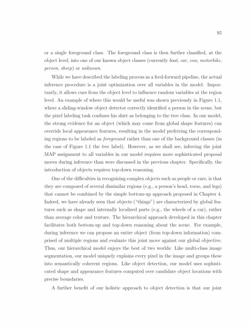
95
or a single foreground class. The foreground class is then further classified, at the
object level, into one of our known object classes (currently boat, car, cow, motorbike,
person, sheep) or unknown.
While we have described the labeling process as a feed-forward pipeline, the actual
inference procedure is a joint optimization over all variables in the model. Impor-
tantly, it allows cues from the object level to influence random variables at the region
level. An example of where this would be useful was shown previously in Figure 1.1,
where a sliding-window object detector correctly identified a person in the scene, but
the pixel labeling task confuses his shirt as belonging to the tree class. In our model,
the strong evidence for an object (which may come from global shape features) can
override local appearance features, resulting in the model preferring the correspond-
ing regions to be labeled as foreground rather than one of the background classes (in
the case of Figure 1.1 the tree label). However, as we shall see, inferring the joint
MAP assignment to all variables in our model requires more sophisticated proposal
moves during inference than were discussed in the previous chapter. Specifically, the
introduction of objects requires top-down reasoning.
One of the difficulties in recognizing complex objects such as people or cars, is that
they are composed of several dissimilar regions (e.g., a person’s head, torso, and legs)
that cannot be combined by the simple bottom-up approach proposed in Chapter 4.
Indeed, we have already seen that objects (“things”) are characterized by global fea-
tures such as shape and internally localized parts (e.g., the wheels of a car), rather
than average color and texture. The hierarchical approach developed in this chapter
facilitates both bottom-up and top-down reasoning about the scene. For example,
during inference we can propose an entire object (from top-down information) com-
prised of multiple regions and evaluate this joint move against our global objective.
Thus, our hierarchical model enjoys the best of two worlds: Like multi-class image
segmentation, our model uniquely explains every pixel in the image and groups these
into semantically coherent regions. Like object detection, our model uses sophisti-
cated shape and appearance features computed over candidate object locations with
precise boundaries.
A further benefit of our holistic approach to object detection is that our joint

96 CHAPTER 5. OBJECT DETECTION AND OUTLINING
Figure 5.1: Contextual information is critical for recognizing small objects. The car inthis image is less than 32× 32 pixels in size and would be difficult to recognize without thesurrounding context.
model over regions and objects allows contextual priors to be encoded through direct
semantic relationships (e.g., cars are usually found on roads, and boats are usually
found on water). These types of relationships are particularly important when ob-
jects are small. Consider, for example, the image in Figure 5.1. Here, a standard
sliding-window object detection algorithm that only considers local features would
have difficulty detecting the cars due to their small size—the largest car in the image
has fewer than 32 × 32 pixels. However, by making use of contextual information
such as proximity to the road and, perhaps, other car-like objects, as well as an
understanding of global scale, we as humans have no trouble identifying the cars.
5.1 Region-based Model for Object Detection
In this section, we present our joint object detection and scene segmentation model.
This model combines scene structure with region and object level semantics in a
coherent energy function. Unlike the previous chapter, which included both geometric
and semantic labels for each region, we restrict our attention here to just the semantic
labels. However, we still maintain the horizon in our model as it constrains on the
location of semantic classes and allows us to encode relative object size.

5.1. REGION-BASED MODEL FOR OBJECT DETECTION 97
5.1.1 Energy Function
Our model builds on the model from the previous chapter, which aims to decompose
a scene into a number (K) of semantically consistent regions. Recall that each pixel
p in the image I is assigned to exactly one region, identified by its region-association
variable Rp ∈ 1, . . . ,K. The r-th region is simply the set of pixels Pr whose region-
association variable equals r, i.e., Pr = p : Rp = r. As in the previous chapter,
we use p and q to denote pixels, and r and s to denote regions. In this chapter, we
introduce the index o to denote objects. Double subscripts indicate pairwise terms
between adjacent entities (e.g., or references the pairwise term between an object o
and a region r adjacent to it).
Regions, while visually coherent, may not encompass entire objects. Indeed, in
Chapter 4 we saw that foreground objects tend to be over-segmented into multiple
regions. We address this complication by allowing an object to be composed of many
regions rather than trying to force dissimilar regions to merge. The object to which
a region belongs is denoted by its object-association variable Or ∈ ∅, 1, . . . , N.Some regions, such as background, do not belong to any object, which we denote by
Or = ∅. Like regions, the set of pixels that comprise the o-th object is denoted by
Po =⋃
r:Or=o Pr. Currently, we do not allow a single region or object to be composed
of multiple disconnected components.
Random variables are associated with the various entities (pixels, regions, objects,
and horizon) in our model. Each pixel has a local appearance feature vector αp ∈ Rn.
Each region has an appearance variable Ar that summarizes the appearance of the
whole region, a semantic class label Sr (such as “road” or “foreground object”), and
an object-association variable Or. Each object, in turn, has an object class label Co
(such as “car” or “pedestrian”). As discussed in Chapter 4, our model also includes
the location of the horizon, which captures global geometry information. Recall,
we assume that the image was taken by a camera with horizontal axis parallel to
the ground and model the horizon vhz ∈ [0, 1] as the normalized row in the image
corresponding to its location. We quantize vhz into the same number of rows as the
image.
We combine the variables in our model into a single coherent energy function

98 CHAPTER 5. OBJECT DETECTION AND OUTLINING
Figure 5.2: An illustration of random variables defined by our joint object detection andscene decomposition model.
that captures the structure and semantics of the scene. The energy function includes
terms for modeling the location of the horizon, region label preferences, region bound-
ary quality, object labels, and contextual relationships between objects and regions.
These terms are described in detail below. The combined energy function has the
form:
E(R,S,O,C, vhz | I,θ) = ψhorizon(vhz) +∑
r
ψregr (Sr, v
hz)
+∑
r,s
ψbdryrs +
∑
o
ψobjo (Co, v
hz) +∑
o,r
ψctxtor (Co, Sr) (5.1)
where for notational clarity the subscripts on the individual energy terms indicate
that they are functions of the pixels (appearance and shape) belonging to the corre-
sponding regions or objects, i.e., ψregr is also a function of Pr, etc. It is assumed that
all terms are conditioned on the observed image I and learned model parameters θ.

5.1. REGION-BASED MODEL FOR OBJECT DETECTION 99
The summation over context terms includes all ordered pairs of adjacent objects and
regions, while the summation over boundary terms is over unordered pairs of regions.
An illustration of the variables in the energy function is shown in Figure 5.2.
The first three energy terms are adapted from the scene decomposition model
of Chapter 4. We briefly review them here:
Horizon term. The ψhorizon term captures the a priori location of the horizon in
the scene and, in our model, is implemented as a log-gaussian
ψhorizon(vhz) = −ηhorizon logN (vhz;µ, σ2) (5.2)
with parameters µ and σ learned from labeled training images.
Knowing the location of the horizon allows us to compute the world height of
an object in the scene. Using the derivation from Hoiem et al. [2008b], it can be
shown that the height yk of an object (or region) in the scene can be approximated
as yk ≈ h vt−vb
vhz−vbwhere h is the height of the camera origin above the ground, and
vt and vb are the row of the top-most and bottom-most pixels in the object/region,
respectively. In our current work, we assume that all images were taken from the
same height above the ground, allowing us to use vt−vb
vhz−vbas a feature in our region and
object terms.
Region term. The region term ψreg in our energy function captures the prefer-
ence for a region to be assigned different semantic labels (currently sky, tree, road,
grass, water, building, mountain, foreground). For convenience we include the vhz
variable in this term to provide information about scene structure. If a region is asso-
ciated with an object, then we constrain the assignment of its class label to foreground
(e.g., a “sky” region cannot be part of a “car” object).
More formally, letNr be the number of pixels in region r, i.e., Nr =∑
p 1Rp = r,and let φr (Ar,Pr) ∈ R
n denote the features for the r-th region (see Section 4.1.3).
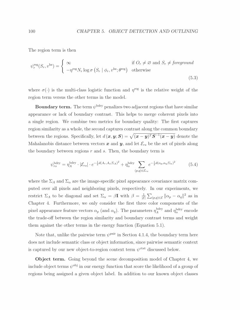
100 CHAPTER 5. OBJECT DETECTION AND OUTLINING
The region term is then
ψregr (Sr, v
hz) =
∞ if Or 6= ∅ and Sr 6= foreground
−ηregNr log σ(Sr | φr, v
hz; θreg)
otherwise
(5.3)
where σ(·) is the multi-class logistic function and ηreg is the relative weight of the
region term versus the other terms in the model.
Boundary term. The term ψbdry penalizes two adjacent regions that have similar
appearance or lack of boundary contrast. This helps to merge coherent pixels into
a single region. We combine two metrics for boundary quality: The first captures
region similarity as a whole, the second captures contrast along the common boundary
between the regions. Specifically, let d (x,y;S) =√
(x− y)T S−1(x− y) denote the
Mahalanobis distance between vectors x and y, and let Ers be the set of pixels along
the boundary between regions r and s. Then, the boundary term is
ψbdryrs = ηbdry
A · |Ers| · e−1
2d(Ar,As;ΣA)2 + ηbdry
α
∑
(p,q)∈Ers
e−1
2d(αp,αq;Σα)2 (5.4)
where the ΣA and Σα are the image-specific pixel appearance covariance matrix com-
puted over all pixels and neighboring pixels, respectively. In our experiments, we
restrict ΣA to be diagonal and set Σα = βI with β = 1|E|
∑
(p,q)∈E ‖αp − αq‖2 as in
Chapter 4. Furthermore, we only consider the first three color components of the
pixel appearance feature vectors αp (and αq). The parameters ηbdryA and ηbdry
α encode
the trade-off between the region similarity and boundary contrast terms and weight
them against the other terms in the energy function (Equation 5.1).
Note that, unlike the pairwise term ψpair in Section 4.1.4, the boundary term here
does not include semantic class or object information, since pairwise semantic context
is captured by our new object-to-region context term ψctxt discussed below.
Object term. Going beyond the scene decomposition model of Chapter 4, we
include object terms ψobj in our energy function that score the likelihood of a group of
regions being assigned a given object label. In addition to our known object classes

5.1. REGION-BASED MODEL FOR OBJECT DETECTION 101
(currently, boat, car, cow, motorbike, person, and sheep), an object (or foreground
region) can take the class label unknown. This unknown class includes objects not
currently explicitly modeled, such as trash cans, street signs, telegraph poles, traffic
cones, bicycles, etc. Similar to the region term, the object term is defined by a logistic
function that maps object-specific features φo
(Po, v
hz, I)∈ R
n to a probability for
each object class. We discuss the construction of these features in Section 5.1.2 below.
Instead of taking the log-likelihood from the logistic function and incorporating
it directly into our energy function, we first perform an important refinement that
acts to normalize this term against information already present in the region layer.
Specifically, since our region layer already identifies foreground regions, we would like
our energy to improve only when we recognize known object classes. We therefore
bias the object term to give zero contribution to the energy for the class unknown.2
Formally, we have
ψobjo (Co, v
hz) = −ηobjNo
(log σ
(Co | φo; θ
obj)− log σ
(unknown | φo; θ
obj))
(5.5)
where No =∑
r:Or=oNr is the number of pixels belonging to the object.
Context term. Intuitively, contextual information which relates objects to their
local background can improve object detection. For example, Heitz and Koller [2008]
showed that detection rates improve by relating “things” (objects) to “stuff” (back-
ground). Our model has a very natural way of encoding such relationships through
pairwise energy terms between objects Co and regions Sr. We do not encode contex-
tual relationships between region classes (i.e., Sr and Ss) although this could also be
done. However, most interesting contextual relationships exist between foreground
objects and their neighboring regions in the scene. Contextual relationships between
two adjacent foreground objects (i.e., Co and Cm) may be beneficial (e.g., people
found on bicycles), but are not considered in this work. Formally, the context term
2Technically, this allows the Or variable to take the value ∅ for unknown foreground regionswithout affecting the energy.

102 CHAPTER 5. OBJECT DETECTION AND OUTLINING
Context Feature Description
Relative Position (8) Orientation of the centroid of region r withrespect to the centroid of object o quantizedinto eight compass directions.
Table 5.1: Summary of the features φor(Po,Pr) used to describe the contextual pairwiserelationship between an object o and adjacent region r.
in the energy function is
ψctxtor (Co, Sr) = −ηctxt log σ
(Co × Sr | φor; θ
ctxt)
(5.6)
where φor (Po,Pr, I) ∈ Rn is a pairwise feature vector for object o and region r, σ(·)
is the multi-class logistic function, and ηctxt weights the strength of the context term
relative to other terms in the energy function. Our context features, summarized in
Table 5.1, simply capture the orientation of the region with respect to the object
allowing us to encode simple preferences such as “on top of”, “next to”, etc.
Since the pairwise context term is between objects and (background) regions it
grows linearly with the number of object classes. This has a distinct advantage over
including a pairwise term between all classes, which would result in quadratic growth.
5.1.2 Object Features
Performing well at object detection requires more than simple aggregated region ap-
pearance features. Indeed, the power of state-of-the-art object detectors comes from
their ability to model localized appearance and general shape characteristics of an
object class. Thus, in addition to raw appearance features (similar to our region-level
appearance features), we append to our object feature vector φo features derived from
such object detection models. We discuss two methods for adapting state-of-the-art
object detector machinery for this purpose.

5.1. REGION-BASED MODEL FOR OBJECT DETECTION 103
Black-box Object Detectors
In the first approach, we treat the object detector as a black-box that returns a score
per (rectangular) candidate window. However, recall that an object in our model
is defined by a contiguous set of pixels Po that can have an arbitrary shape, not
necessarily a rectangular window. In the black-box approach, we naively place a
bounding box (at the correct aspect ratio) around these pixels and classify the entire
contents of the box. To make classification more robust we search candidate windows
in a small neighborhood (defined over scale and position) around this bounding box,
and take as our feature the output of highest scoring window. Any state-of-the-
art object detection algorithm can be used in the black-box model allowing this
approach to easily take advantage of advances in object detection technology. In
our experiments, we test this approach using the HOG detector of Dalal and Triggs
[2005], which learns a linear support vector machine (SVM) classifier over feature
vectors constructed by computing histograms of gradient orientations in fixed-size
overlapping cells within the candidate window (see Chapter 2).
An important practical consideration is how to interface the black-box object
detector (for which we may only have an external executable) to our model. It appears
that we have a “chicken and egg” situation: Before running inference we do not know
which pixels belong to objects, however, we cannot run inference without computing
features over the objects. Since our inference procedure (discussed in Section 5.2.1
below) is proposal-move based, one solution is to make a call to the object detector
each time we propose a new object. However, this solution incurs significant overhead
resulting in a dramatic increase in running time.
A more pragmatic approach is to first run the (external) object detector over
the entire image to collect object detection candidate windows. This is the usual
operating mode of an object detector. We can then limit the location of objects in
the scene to the subset of windows returned by the external object detector. This, in
effect, forces ψobjo to take the value ∞ whenever Po does not sufficiently overlap with
a candidate detection. Note that we can tune the threshold of the object detector to
increase the number of detection candidates making it more likely that we cover all
true objects in the scene.

104 CHAPTER 5. OBJECT DETECTION AND OUTLINING
Integrated Object Detectors
Despite its simplicity, the black-box approach is somewhat unsatisfying in that many
of the pixels within the bounding box being evaluated are not actually part of the
object. For example, consider an L-shaped region. To a black-box approach, this is
indistinguishable from a full bounding box positioned tightly around the “L”.
A more elegant approach is to mask out all pixels not belonging to the object.
In our implementation, we use a soft mask that attenuates the intensity of pixels
outside of the object boundary as a function of their distance to the boundary (see
Figure 5.3). This has the dual advantage of preventing hard edge artifacts and being
less sensitive to small segmentation errors. Consider, for example, the true-positive
window for detecting cars shown in Figure 5.3(c). Here, with the correct region mask,
the effect of masking (either soft or hard) is not significant. However, in the case of
a false-positive window (e.g., Figure 5.3(h)), applying a hard mask introduces strong
edge artifacts that may cause the window to be incorrectly classified, whereas the soft
mask produces a region that is unlikely to be confused with a car.
The soft mask can be thought of as a matrix the same size as the window being
classified. It is generate by setting entries corresponding to the pixels in the object to
one, and all other entries to zero. (This gives the hard mask.) We then dilate the mask
by 7 pixels and apply a Gaussian smoothing filter with a radius of 15 pixels. This
ensures a gradual decay in pixel intensity beyond the object boundary. Finally, we
multiply the image color values by the soft mask to get the window for classification.
The soft mask is used at both training and test time to ensure consistency between
training and test examples.3
Many different object detectors can be adapted for this more integrated approach,
and in our experiments, we evaluate the approach using the patch-based approach of
Torralba et al. [2004a,b]. Here, features are extracted by matching small rectangu-
lar patches at fixed locations within the masked window and combining these weak
3At training time we have ground truth labels for pixels belonging to regions and can thereforegenerate the masks. It is also possible to use standard black-box training methods which do not haveaccess to pixel masks and still apply the trained classifier to masked regions during test. However,we did not evaluate performance under this regime.

5.1. REGION-BASED MODEL FOR OBJECT DETECTION 105
(c) true-positive window (h) false-positive window
(a) hard regionmask
(d) image withhard window
(e) edges withhard window
(i) image withhard window
(j) edges withhard window
(b) soft regionmask
(f) image withsoft window
(g) edges withsoft window
(k) image withsoft window
(l) edges withsoft window
Figure 5.3: Illustration of soft masks for proposed object regions. Using a hard regionmask is problematic since it introduces edge artifacts that can result in misclassification ofthe window. These artifacts are reduced when a soft mask is used.
responses using boosted decision trees. Object appearance and shape are captured
by matching the patches on both the original (intensity) image and the edge-filtered
image. A more complete description of this patch-based object detector is provided
in Section 2.2.3.
For both black-box and integrated approaches, we append the score (for each
object category) from the object detection classifiers—linear SVM for HOG-bases or
boosted decision trees for patch-based—to the object feature vector φo. Our object-
level features are summarized in Table 5.2.
Image Resolution
An important parameter for object detection is the base scale at which features are
extracted. Scale-invariance is usually achieved by successively down-sampling the
image. Below the base-scale, feature matching becomes inaccurate, so most detectors
will only find objects above some minimum size. Clearly there exists a trade-off

106 CHAPTER 5. OBJECT DETECTION AND OUTLINING
Object Feature Description
Appearance (51) Aggregated region appearance: Mean and standarddeviation of the 17-dimensional filter responses andboosted classifier score for each pixel in the object, andlog-determinant of the appearance covariance matrix ΣA
o
computed over all pixels in the object.
Boundary Contrast (4) Measure of the contrast along the boundary of the objectrelative to its interior.
Shape (19) Basic region shape such as size and extent (relative toimage dimensions), perimeter length and “straightness”,and first- and second-order shape moments. These fea-tures also include binary indicators capturing whetherthe region has been truncated by the edge, top, or bot-tom of the image.
Geometry (10) Like its region counterpart, these features capture therelative location of the object with respect to the horizonvhz and include the percentage of pixels in the objectabove and below the horizon; the spread of pixels aboutthe horizon (i.e., mean distance above and below thehorizon). We also add the term vt−vb
vhz−vbwhere vt and
vb are the topmost and bottom most row in the object,respectively. This captures the relative height of objectsin the scene.
Detector Score (1) Score from running trained object detector on the pix-els belonging to the object. The score can either bederived by running a black-box detector on a boundingbox covering the pixels in the object, or from an inte-grated object detector applied to a masked-window asshown in Figure 5.3.
Table 5.2: Summary of the features φo(Po, vhz, I) used to describe an object in our model.
The first five sets of features are extended variants of the region features described in theprevious chapter. The last feature is a powerful top-down feature that captures global cues(such as shape and localized appearance).
5.2. INFERENCE AND LEARNING 107
between the desire to detect small objects, feature quality, and computational cost.
To reduce the computational burden of running our full scene decomposition model
on high-resolution images while still being able to identify small objects, we employ a
multi-scale approach. In this approach, we run our scene decomposition algorithm on
a low-resolution (320×240) version of the scene, but extract features from the original
high-resolution version (if available in the dataset).4 That is, when we extract object-
detector features we map the object pixels Po onto the original image and extract our
features at the higher resolution.
5.2 Inference and Learning
In Section 4.2 we developed the inference and learning procedures for the basic scene
decomposition model. In this section we briefly review those methods and describe
the extensions necessitated by the inclusion of object variables into our model.
5.2.1 Inference
We use a modified version of the hill-climbing inference algorithm described in Chap-
ter 4, which uses multiple over-segmentations to propose large moves in the energy
space. An overview of this procedure is shown in Algorithm 5.1. As in Chapter 4, we
initialize the variables in our model by segmenting the image using an off-the-shelf
unsupervised segmentation algorithm (e.g., mean-shift [Comaniciu and Meer, 2002]).
We then run inference using a two-phased approach.
In the first phase, we want to build up a good set of initial regions before trying
to classify them as objects. Thus, we remove the object variables O and C, and
corresponding energy terms ψobj and ψctxt, from the model, and perform inference
over the reduced state space. In this phase, the algorithm behaves exactly as in the
previous chapter by iteratively proposing re-assignments of pixels to regions (variables
R) and recomputing the optimal (conditional) assignment to the remaining variables
(in this case, S and vhz). If the overall energy for the new configuration is lower, then
4In our experiments, high-resolution images were only available for the Street Scenes dataset.

108 CHAPTER 5. OBJECT DETECTION AND OUTLINING
the move is accepted, otherwise the previous configuration is restored and the algo-
rithm proposes a different move. The algorithm proceeds until no further reduction
in energy can be found after exhausting all proposal moves from a predefined set (see
Section 5.2.2).
In the second phase, we introduce object variables over all foreground regions.
Initially, the object class variable is set to unknown so that this operation does not
affect the overall energy. We then iteratively propose merges and splits of both
regions and objects (variables R and O) as well as top-down proposal moves (see
Section 5.2.2 below) to generate new regions from sliding-window object candidates
(again, affecting both R and O). After a move is proposed, we recompute the optimal
assignment to the remaining variables (S, C and vhz). As in the first phase, this
process repeats until the energy cannot be reduced by any of the proposal moves.
Since only part of the scene is changing during any iteration we only need to
recompute the features and energy terms for the entities affected by a move. However,
inference is still slow given the sophisticated features that need to be computed and
the large number of moves considered. To improve running time, we leave the context
terms ψctxt out of the model until the last iteration through the proposal moves. This
allows us to maximize each region term independently during each proposal step. We
then greedily update vhz after the region labels have been inferred. After introducing
the context term, we use max-product belief propagation to infer the optimal joint
assignment to S and C.
5.2.2 Proposal Moves
We now describe the set of pixel and region proposal moves considered by our al-
gorithm. These moves are relative to the current best scene decomposition and are
designed to take large steps in the energy space to avoid local minima. As discussed
above, each move is accepted if it results in a lower overall energy after inferring the
optimal assignment to the remaining variables.
The main set of pixel moves are described in Chapter 4 but briefly repeated here

5.2. INFERENCE AND LEARNING 109
Algorithm 5.1: Scene Decomposition with Objects Inference.
Input : I // image1
θ // model parameters2
Output: R,S,O,C, and vhz // scene decomposition3
// phase one:
generate over-segmentation dictionary Ω (see § 4.2.1)4
initialize variables R, S and vhz5
repeat6
foreach pixel proposal move do7
re-assign region-association variables R (see § 4.2.1)8
update region and boundary features φ9
run inference over region variables S and horizon vhz10
compute total energy E of new assignments11
if (E < Emin) then12
accept move and set Emin = E13
else14
reject move15
end16
end foreach17
until Emin does not change18
// phase two:
generate top-down object dictionary (see § 5.2.2)19
initialize variables O and C20
repeat21
foreach pixel or region proposal move do22
re-assign region-association R or object-association variables O23
update region, boundary and object features φ24
run inference over region and object variables (S,C) and horizon vhz25
compute total energy E of new assignments26
if (E < Emin) then27
accept move and set Emin = E28
else29
reject move30
end31
end foreach32
until Emin does not change33
return R,S,O,C, and vhz34

110 CHAPTER 5. OBJECT DETECTION AND OUTLINING
for completeness. The most basic move is to merge two adjacent regions. More so-
phisticated moves involve local re-assignment of pixels to neighboring regions. These
moves are proposed from a precomputed dictionary of image segments Ω. The dic-
tionary is generated by varying the parameters of an unsupervised over-segmentation
algorithm (in our case mean-shift [Comaniciu and Meer, 2002]) and adding each seg-
ment ω to the dictionary. During inference, these segments are used to propose a
re-assignment of all pixels in the segment to a neighboring region or creation of new
region. As shown in Chapter 4, these bottom-up proposal moves work well for back-
ground classes, but tend to result in over-segmentation of foreground objects that
have heterogeneous appearance. For example, one would not expect the wheels and
body of a car to be grouped together by a bottom-up approach.
An analogous set of moves can be used for merging two adjacent objects or assign-
ing regions to objects. For example, merging two adjacent objects o and s involves
re-assigning all regions r : Or = s to o, or creating a new object by assigning Or
to a new object for some region r. However, if an object is decomposed into multi-
ple regions, this bottom-up approach is problematic as multiple such moves may be
required to produce a complete object. When performed independently, these moves
are unlikely to improve the energy. We get around this difficulty by introducing a
new set of powerful top-down proposal moves based on object detection candidates.
Here, we use precomputed candidates from a sliding-window detector to propose new
foreground regions with corresponding object variable.5 In the case of the black-box
approach, described in Section 5.1.2, these are the only candidate objects that we
allow.
Directly proposing moves involving all pixels inside the bounding box obtained
from the sliding-window detector for the candidate object, is likely to result in an
increase in energy due to the introduction of artificial boundaries into the scene de-
composition. We implement two solutions to this problem. First, instead of proposing
a move over all pixels in the bounding box, we propose move that re-assign only the
pixels inside the set of segments (from our segment dictionary Ω) fully contained
within the bounding box. An illustration of this procedure is shown in Figure 5.4.
5In our experiments, we take as candidates the top twenty detections for each object category.
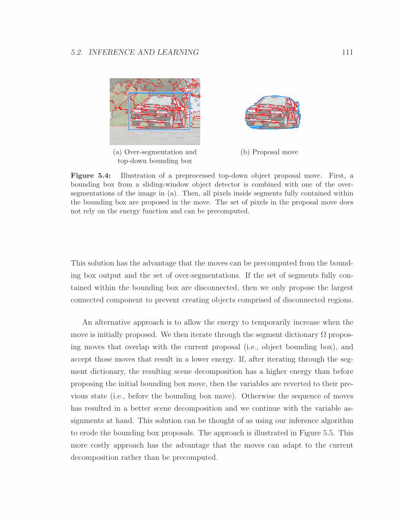
5.2. INFERENCE AND LEARNING 111
(a) Over-segmentation andtop-down bounding box
(b) Proposal move
Figure 5.4: Illustration of a preprocessed top-down object proposal move. First, abounding box from a sliding-window object detector is combined with one of the over-segmentations of the image in (a). Then, all pixels inside segments fully contained withinthe bounding box are proposed in the move. The set of pixels in the proposal move doesnot rely on the energy function and can be precomputed.
This solution has the advantage that the moves can be precomputed from the bound-
ing box output and the set of over-segmentations. If the set of segments fully con-
tained within the bounding box are disconnected, then we only propose the largest
connected component to prevent creating objects comprised of disconnected regions.
An alternative approach is to allow the energy to temporarily increase when the
move is initially proposed. We then iterate through the segment dictionary Ω propos-
ing moves that overlap with the current proposal (i.e., object bounding box), and
accept those moves that result in a lower energy. If, after iterating through the seg-
ment dictionary, the resulting scene decomposition has a higher energy than before
proposing the initial bounding box move, then the variables are reverted to their pre-
vious state (i.e., before the bounding box move). Otherwise the sequence of moves
has resulted in a better scene decomposition and we continue with the variable as-
signments at hand. This solution can be thought of as using our inference algorithm
to erode the bounding box proposals. The approach is illustrated in Figure 5.5. This
more costly approach has the advantage that the moves can adapt to the current
decomposition rather than be precomputed.

112 CHAPTER 5. OBJECT DETECTION AND OUTLINING
(a) Starting decomposition (b) Proposed bounding box (c) Final eroded move
Figure 5.5: Illustration of eroding a top-down bounding box move. The proposed bound-ing box move in (b) is likely to cause the energy to increase above the energy of startingdecomposition (a) due to the region boundary artifacts introduced by the move. After run-ning inference the bounding box is eroded resulting in lower energy scene decompositionin (c). Region boundaries are shown in black. Since the proposal move makes use of thecurrent scene decomposition and energy function, the set of pixels in the final eroded movecannot be predetermined.
5.2.3 Learning
Object detectors are learned separately using black-box training procedures and
their output provided as input features to the combined model (as discussed in Sec-
tion 5.1.2). Then, as in Chapter 4, we learn the parameters of our model from labeled
training data in a piecewise fashion. First, the individual terms are learned using an
ℓ2-regularized maximum-likelihood objective for the subset of variables within each
term. The relative weights (ηreg, ηobj, etc.) between the terms are learned through
cross-validation on a subset of the training data to optimize object detection perfor-
mance (as measured by area under the precision-recall curve).
For both the base object detectors and the parameters of the region and object
terms, we use a closed-loop learning technique where we first learn an initial set of
parameters from training data. We then run inference on our training set and record
mistakes made by the algorithm (false-positives for object detection and incorrect re-
gion proposal moves for the full algorithm as described in Section 4.2.2). We augment
the training data with these mistakes and re-train each term. This process gives a
significant improvement to the final results.
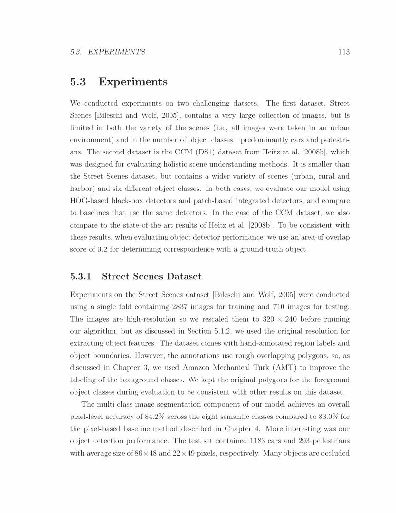
5.3. EXPERIMENTS 113
5.3 Experiments
We conducted experiments on two challenging datsets. The first dataset, Street
Scenes [Bileschi and Wolf, 2005], contains a very large collection of images, but is
limited in both the variety of the scenes (i.e., all images were taken in an urban
environment) and in the number of object classes—predominantly cars and pedestri-
ans. The second dataset is the CCM (DS1) dataset from Heitz et al. [2008b], which
was designed for evaluating holistic scene understanding methods. It is smaller than
the Street Scenes dataset, but contains a wider variety of scenes (urban, rural and
harbor) and six different object classes. In both cases, we evaluate our model using
HOG-based black-box detectors and patch-based integrated detectors, and compare
to baselines that use the same detectors. In the case of the CCM dataset, we also
compare to the state-of-the-art results of Heitz et al. [2008b]. To be consistent with
these results, when evaluating object detector performance, we use an area-of-overlap
score of 0.2 for determining correspondence with a ground-truth object.
5.3.1 Street Scenes Dataset
Experiments on the Street Scenes dataset [Bileschi and Wolf, 2005] were conducted
using a single fold containing 2837 images for training and 710 images for testing.
The images are high-resolution so we rescaled them to 320 × 240 before running
our algorithm, but as discussed in Section 5.1.2, we used the original resolution for
extracting object features. The dataset comes with hand-annotated region labels and
object boundaries. However, the annotations use rough overlapping polygons, so, as
discussed in Chapter 3, we used Amazon Mechanical Turk (AMT) to improve the
labeling of the background classes. We kept the original polygons for the foreground
object classes during evaluation to be consistent with other results on this dataset.
The multi-class image segmentation component of our model achieves an overall
pixel-level accuracy of 84.2% across the eight semantic classes compared to 83.0% for
the pixel-based baseline method described in Chapter 4. More interesting was our
object detection performance. The test set contained 1183 cars and 293 pedestrians
with average size of 86×48 and 22×49 pixels, respectively. Many objects are occluded
114 CHAPTER 5. OBJECT DETECTION AND OUTLINING
Patch-based HOG-based
Baseln. Unary Ctxt. Baseln. Unary Ctxt.
Car 0.40 0.55 0.56 0.35 0.58 0.57Pedestrian 0.15 0.22 0.21 0.37 0.35 0.35Mean 0.28 0.39 0.39 0.36 0.47 0.46
Table 5.3: Object detections results for the Street Scenes dataset [Bileschi and Wolf, 2005].Performance is measured by area under the precision-recall curve (average precision).
making this a very difficult dataset.
Since our algorithm produces MAP estimation for the scene we cannot simply
generate a precision-recall curve by varying the object classifier threshold as is usual
for reporting object detection results. Instead, we take the max-marginals for each
Co variable at convergence of our algorithm and sweep over thresholds for each object
class separately to generate a curve. An attractive aspect of this approach is that our
method does not have overlapping candidates and hence does not require arbitrary
post-processing such as non-maximal suppression of sliding-window detections.
Our results are summarized in Table 5.3. We include a comparison against two
baseline sliding-window approaches. For the patch-based detector, our method im-
proves over the baseline for both object categories. Our method also shows significant
improvement over the HOG baseline for car detection. Interestingly, for pedestrian
detection, our method shows only comparable performance to the HOG baseline.
However, this should not be surprising since the HOG detector was specifically engi-
neered for the task of pedestrian detection. Furthermore, as we discuss below, context
is not as helpful here due to the limited variety of scenes.
Complete precision-recall curves are shown in Figure 5.6 for both the patch-based
and HOG-based detectors. Notice that our method does not achieve 100% recall
(even at low precision) due to the curves being generated from the MAP assignment
in which pixels have already been grouped into regions. Unlike the baselines, this
forces only one candidate object per region. However, by trading off the strength
(and hence operating point) of the energy terms in our model it is possible to increase
the maximum recall for a given object class at the expense of precision.
Removing the pairwise context term does not have a significant effect on our

5.3. EXPERIMENTS 115
Patch-based
0 0.1 0.2 0.3 0.4 0.5 0.6 0.7 0.8 0.9 10
0.1
0.2
0.3
0.4
0.5
0.6
0.7
0.8
0.9
1
recall
pre
cis
ion
0 0.1 0.2 0.3 0.4 0.5 0.6 0.7 0.8 0.9 10
0.1
0.2
0.3
0.4
0.5
0.6
0.7
0.8
0.9
1
recall
pre
cis
ion
(a) Cars (b) Pedestrians
0 0.1 0.2 0.3 0.4 0.5 0.6 0.7 0.8 0.9 10
0.1
0.2
0.3
0.4
0.5
0.6
0.7
0.8
0.9
1
recall
pre
cis
ion
sliding−window
region−based
(c) Combined cars and pedestrians
HOG-based
0 0.1 0.2 0.3 0.4 0.5 0.6 0.7 0.8 0.9 10
0.1
0.2
0.3
0.4
0.5
0.6
0.7
0.8
0.9
1
recall
pre
cis
ion
0 0.1 0.2 0.3 0.4 0.5 0.6 0.7 0.8 0.9 10
0.1
0.2
0.3
0.4
0.5
0.6
0.7
0.8
0.9
1
recall
pre
cis
ion
(a) Cars (b) Pedestrians
0 0.1 0.2 0.3 0.4 0.5 0.6 0.7 0.8 0.9 10
0.1
0.2
0.3
0.4
0.5
0.6
0.7
0.8
0.9
1
recall
pre
cis
ion
sliding−window
region−based
(c) Combined cars and pedestrians
Figure 5.6: Object detection precision-recall curves for patch-based (left) and HOG-based(right) detectors on the Street Scenes dataset [Bileschi and Wolf, 2005]. Plots (a) and (b)show individual PR curves for each object; plot (c) shows combined curve.
results. This is due to the encoding of some context through the region term (e.g., the
relative position of the horizon) and the fact that all images were of urban scenes.
Hence most detections—both true and false—were supported by road regions and
surrounded by buildings. As we shall see, context does play an important role when
we consider the more varied scenes in the CCM dataset.
Example output for a typical image from our dataset is shown in Figure 5.7.
The example shows the original image, semantic overlay with object outlines, scene
decomposition (in terms of regions), and estimated horizon location. Notice how the
two foreground regions get grouped together into a single “car” object.
We also show a selection of qualitative object detection results in Figure 5.8. Here,
we only show the original image and semantic overlay for each example. Notice that
our algorithm is able to detect multiple (adjacent) objects per image. In some cases,
for example, the scene containing two cars in the first column and second row, the

116 CHAPTER 5. OBJECT DETECTION AND OUTLINING
Figure 5.7: Example output from our joint scene decomposition and object detection al-gorithm. Shown are: (a) the original image, (b) semantic overlay (including object outlines),(c) decomposition by region, and (d) estimated location of horizon.
algorithm incorrectly groups parts of one object with the adjacent object. However,
as can be seen in the other examples, we generally get very good boundaries for cars.
Pedestrians are much more difficult in this dataset, and their small size makes it hard
to obtain precise outlines even when correctly detected (e.g., bottom-right example
in Figure 5.8).
5.3.2 Cascaded Classification Models Dataset
Our second set of experiments were conducted on the more diverse, but smaller CCM
dataset [Heitz et al., 2008b]. Here we conducted five-fold cross-validation on the 422
images and report object detection results averaged across the five folds.
Again, we compare our approach to the HOG-based and patch-based baselines.
However, for the HOG-based baseline we use post-processed detection candidates from
the independent method of Heitz et al. [2008b] rather than directly from the Dalal and
Triggs [2005] detector. This produces a significantly stronger baseline. Aggregated
results from running our inference procedure on the five evaluation folds are shown
in Table 5.4. The table includes the number of instances, precision, and recall for each
object category individually and combined across all object categories (i.e., weighted
average). As can be seen, our model favors high precision at the expense of recall
for some of the more difficult object categories (e.g., pedestrians and boats). That
is, objects that get labeled by our inference procedure tend to be correct. However,

5.3. EXPERIMENTS 117
Figure 5.8: Qualitative object detection results for the Street Scenes dataset [Bileschiand Wolf, 2005]. Each example show original image (left) and overlay colored by semanticclass and detected objects (right).
many of the objects in the dataset are missed by our algorithm at this high-precision
operating point.
As discussed previously, there is a trade-off between precision and recall that can
be tuned by modifying the weight of the object terms in the energy function. For
example, setting the weight for one of the object terms very high will result in more
proposal moves being accepted for that object category, which, in turn, will result in
higher recall. Note, however, that unlike the standard sliding-window approach to
object detection, we do not allow overlapping detections and therefore may still not be
able to achieve 100% recall (for example, if a large high-scoring false-positive overlaps

118 CHAPTER 5. OBJECT DETECTION AND OUTLINING
Obj. Count Recall Precision
Boat 94 0.15 0.82Car 148 0.23 0.79Cow 127 0.37 0.92Motorbike 54 0.31 0.94Person 240 0.10 0.83Sheep 141 0.40 0.95Combined 804 0.24 0.87
Table 5.4: Precision and recall for each object category calculated on the MAP assign-ment, i.e., on objects detected after convergence of inference. Results were generated usingHOG-based detectors on the CCM dataset [Heitz et al., 2008b].
with a smaller true-positive detection). In these experiments we evaluate the trade-off
between precision and recall for each object category by generating precision-recall
curves based on scores obtained from the top-down proposal moves. These moves are
derived from the same set of bounding boxes that are used to generate the baseline
results. Specifically, after our inference algorithm converged, we iterated over each
top-down object candidate and performed a single max-product message passing step
between the object and its neighbors.6 The score for each move is determined from
the beliefs obtained from this single message passing step, and the precision-recall
curve plotted by thresholding on this score.
Our results are summarized, in terms of average precision, in Table 5.5 with full
precision-recall curves shown in Figure 5.9. The curves include the MAP operating
point of our algorithm (from Table 5.4) for the HOG-based object detection method.
For the integrated patch-based detectors, our method significantly improves over the
baseline for all six object classes. However, for the strong HOG-based approach
(with post-processed scores from Heitz et al. [2008b]), our approach improves over
the baseline for four of the six object classes, and is only marginally better than the
CCM results on average. We attribute this to the very strong baseline used, and as
we saw in the Street Scenes results, the fact that the HOG detector was specifically
engineered to work well on pedestrians, which is our weakest category.
6We do this rather than full inference for efficiency. Note, also, that since inference had convergedat this stage, none of the proposal moves can result in a decrease in energy.

5.3. EXPERIMENTS 119
Patch-based HOG-based
Baseln. Unary Ctxt. Indep. Unary Ctxt. CCM
Boat 0.19 0.40 0.45 0.31 0.52 0.53 0.48Car 0.23 0.40 0.45 0.55 0.47 0.52 0.58Cow 0.30 0.50 0.55 0.49 0.52 0.59 0.53Motorbike 0.20 0.49 0.58 0.57 0.70 0.70 0.65Person 0.20 0.28 0.29 0.53 0.36 0.39 0.55Sheep 0.19 0.53 0.55 0.39 0.53 0.57 0.45Mean 0.22 0.43 0.48 0.47 0.52 0.55 0.54
Table 5.5: Object detections results for the CCM dataset [Heitz et al., 2008b]. Per-formance is measured by area under the precision-recall curve (average precision). Theindependent and CCM results are taken from Heitz et al. [2008b].
There is a clear advantage in using contextual information in this dataset. This is
due to the strong correlation between objects and their environments: Boats are found
on water, cars on roads, and sheep on grass. The CCM framework (for the HOG-based
detector) also makes use of context by constructing auxiliary object features from
other computer vision tasks (multi-class image labeling and scene categorization).
However, our unified model allows tighter coupling of context and results in slightly
better performance. It also provides object outlines, which the other methods do not.
Some qualitative results are shown in Figure 5.10. The quality of the outlines is
outstanding and our method is even able to correctly detect difficult objects such as
the small car in the second row and the boat in the last row. Some outlines are not
perfect, for example the person walking her dog, and we miss one of the people in
the top-left image (a consequence of our model operating at high precision). Other—
more dramatic—failure modes are shown in Figure 5.11. These vary from missing
objects completely to producing incorrect object labels. Some failures come from
misclassification of unknown objects, portions of which may resemble known object
categories, such as the bus in Figure 5.11(g). Other errors are caused by incorrect
semantic labels at the region level. For example, our model does not handle reflections
and shadows well and is confused by them in the image of the car in Figure 5.11(h).
Here, the object term has difficulty overcoming the strong beliefs of the region terms.
In most cases, the failure modes could be corrected with stronger object models.

120 CHAPTER 5. OBJECT DETECTION AND OUTLINING
Patch-based
0 0.1 0.2 0.3 0.4 0.5 0.6 0.7 0.8 0.9 10
0.1
0.2
0.3
0.4
0.5
0.6
0.7
0.8
0.9
1
recall
pre
cis
ion
0 0.1 0.2 0.3 0.4 0.5 0.6 0.7 0.8 0.9 10
0.1
0.2
0.3
0.4
0.5
0.6
0.7
0.8
0.9
1
recall
pre
cis
ion
0 0.1 0.2 0.3 0.4 0.5 0.6 0.7 0.8 0.9 10
0.1
0.2
0.3
0.4
0.5
0.6
0.7
0.8
0.9
1
recall
pre
cis
ion
(a) Boats (b) Cars (c) Cows
0 0.1 0.2 0.3 0.4 0.5 0.6 0.7 0.8 0.9 10
0.1
0.2
0.3
0.4
0.5
0.6
0.7
0.8
0.9
1
recall
pre
cis
ion
0 0.1 0.2 0.3 0.4 0.5 0.6 0.7 0.8 0.9 10
0.1
0.2
0.3
0.4
0.5
0.6
0.7
0.8
0.9
1
recall
pre
cis
ion
0 0.1 0.2 0.3 0.4 0.5 0.6 0.7 0.8 0.9 10
0.1
0.2
0.3
0.4
0.5
0.6
0.7
0.8
0.9
1
recall
pre
cis
ion
(d) Motorbikes (e) People (f) Sheep
0 0.1 0.2 0.3 0.4 0.5 0.6 0.7 0.8 0.9 10
0.1
0.2
0.3
0.4
0.5
0.6
0.7
0.8
0.9
1
recall
pre
cis
ion
baseline
unary only
with context
(h) Combined objects
HOG-based
0 0.1 0.2 0.3 0.4 0.5 0.6 0.7 0.8 0.9 10
0.1
0.2
0.3
0.4
0.5
0.6
0.7
0.8
0.9
1
recall
pre
cis
ion
0 0.1 0.2 0.3 0.4 0.5 0.6 0.7 0.8 0.9 10
0.1
0.2
0.3
0.4
0.5
0.6
0.7
0.8
0.9
1
recall
pre
cis
ion
0 0.1 0.2 0.3 0.4 0.5 0.6 0.7 0.8 0.9 10
0.1
0.2
0.3
0.4
0.5
0.6
0.7
0.8
0.9
1
recall
pre
cis
ion
(a) Boats (b) Cars (c) Cows
0 0.1 0.2 0.3 0.4 0.5 0.6 0.7 0.8 0.9 10
0.1
0.2
0.3
0.4
0.5
0.6
0.7
0.8
0.9
1
recall
pre
cis
ion
0 0.1 0.2 0.3 0.4 0.5 0.6 0.7 0.8 0.9 10
0.1
0.2
0.3
0.4
0.5
0.6
0.7
0.8
0.9
1
recall
pre
cis
ion
0 0.1 0.2 0.3 0.4 0.5 0.6 0.7 0.8 0.9 10
0.1
0.2
0.3
0.4
0.5
0.6
0.7
0.8
0.9
1
recall
pre
cis
ion
(d) Motorbikes (e) People (f) Sheep
0 0.1 0.2 0.3 0.4 0.5 0.6 0.7 0.8 0.9 10
0.1
0.2
0.3
0.4
0.5
0.6
0.7
0.8
0.9
1
recall
pre
cis
ion
baseline (Heitz et al., 2008)unary only
with context
CCM (Heitz et al., 2008)MAP operating point
(g) Combined objects
Figure 5.9: Object detection precision-recall curves for patch-based (left) and HOG-based(right) detectors on the CCM dataset [Heitz et al., 2008b]. Plots (a)-(f) show individualPR curve for each object category; plot (g) shows combined curve. The HOG-based plotsinclude the operating point for the MAP assignment indicated by a diamond (⋄).
5.4 Chapter Summary
In this chapter, we have presented a hierarchical model for joint object detection
and image segmentation. Our model builds on the scene decomposition model of
the previous chapter and overcomes many of the problems associated with trying to
combine the related computer vision tasks of object detection and multi-class image
labeling. The main contribution of our model is that it explains every pixel and
enforces consistency between random variables from the different tasks. We achieve
this by representing the scene hierarchically, where pixels are associated with regions,

5.4. CHAPTER SUMMARY 121
and regions are associated with objects. A major benefit of this representation is that
it avoids ad hoc decisions inherent in sliding-window object detectors such as post-
processing to remove overlapping detection candidates. Furthermore, our model is
encapsulated in a modular energy function that can be easily analyzed and improved
as new computer vision technologies become available.
Our method is able to incorporate object features from existing state-of-the-art
object detector frameworks through two mechanisms: Either as external black-box
algorithms or tightly coupled within our inference procedure. The black-box approach
makes it very easy to adapt to the latest algorithms, but limits the object candidates
that we can consider. The integrated approach is not limited to predetermined object
candidates, but requires additional work in integrating the feature computation and
classification methods from the object detectors into our code.
The output of our model is a MAP estimate of the scene structure that includes
annotated regions and objects. We believe that this is the desired output of a scene
understanding algorithm (unless part of some larger pipeline) since it commits us to a
consistent interpretation of the scene. The implication, however, is that our algorithm
operates at a single point on the precision-recall curve. This makes comparison to
existing approaches for object detection difficult, since the standard performance
metric computes area under the precision-recall curve. To get around this difficulty,
we compared precision-recall curves based on scoring proposal moves (and also report
the single operating point from the MAP output).
Finally, we showed how the greedy inference procedure from Chapter 4 could be
extended with top-down proposal moves, which are better suited for finding objects.
The top-down moves were generated from preprocessing step that collected candidate
bounding boxes produced when running a sliding-window detector over the image.
There are many ways in which these bounding boxes can be used to propose object
moves, and we discussed two of them. In both approaches, the bounding box is
pruned in some way to obtain a better object outline. Other interesting approaches
along these lines, which we did not discuss, are to use image editing techniques from
the computer graphics community for cropping objects out of images, e.g., [Rother

122 CHAPTER 5. OBJECT DETECTION AND OUTLINING
et al., 2004, Lempitsky et al., 2009a]. These techniques could produce very good pro-
posal moves (at a small additional computational cost) when the candidate detections
correctly encompass an object.

5.4. CHAPTER SUMMARY 123
Figure 5.10: Qualitative object detection results for the CCM dataset [Heitz et al.,2008b]. Each example shows the original image (left) and overlay colored by semantic classand detected objects (right).

124 CHAPTER 5. OBJECT DETECTION AND OUTLINING
(a) Failed to detect some objects (b) Adjacent objects merged together
(c) Adjacent objects merged together (d) Incorrect object label
(e) Incorrect object boundary (f) Failed to erode proposal move
(g) Unknown bus object (h) Semantic labeling failure
Figure 5.11: Failure modes of our scene understanding algorithm. Each example showsthe original image (left) and overlay colored by semantic class and detected objects (right).For example, (a) shows two missed person detections; (d) shows a cow incorrectly classifiedas a sheep; and (h) shows the hood of a car incorrectly labeled as water.

Chapter 6
Scene Reconstruction: From
Semantics to Geometry
Recovering the 3D structure of a scene from a single image is a fundamental problem
in computer vision that has application in robotics, surveillance and general scene
understanding—if we can estimate scene structure then we can better understand
the scene by knowing the 3D relationships between the objects within it. However,
estimating structure from raw image features is extremely difficult since local appear-
ance is insufficient to resolve depth ambiguities (e.g., sky and water regions in an
image can have similar appearance but dramatically different geometric placement
within the scene). In this chapter, we demonstrate how semantic understanding of a
scene, such as that obtained from our region-based scene understanding framework,
can be used to better interpret the 3D structure of a scene, resulting in a complete
understanding of regions, objects and geometry.
Producing spatially plausible 3D reconstructions of a scene from monocular im-
ages annotated with geometric cues, such as horizon location, vanishing points, and
region/surface boundaries, is a well understood problem [Criminisi et al., 2000]. In
the first part of this chapter, we show how our region-based decomposition of the
scene provides such geometric cues automatically and can be used to generate novel
3D views of the scene. Our approach is very simple and obtains its power from our
region-based decomposition rather than sophisticated features tuned for the task.
125

126 CHAPTER 6. SCENE RECONSTRUCTION
Figure 6.1: Example output from our semantically-aware depth estimation model showinghow semantic class prediction (center) strongly informs depth perception (right). Semanticclasses are shown overlayed on image. Depth indicated by color map (red is more distant).
Nevertheless, the results from our approach are surprisingly good. Since our model
does not provide true depth estimates our goal here is to produce planar geometric
reconstructions of each region with accurate relative distances rather than absolute
distance. Given an estimate of the distance between any two points in the scene, our
3D reconstruction can then be scaled to the appropriate size.
Determining absolute (rather than relative) depths from monocular images is a
notoriously difficult task—even for humans—and has been the subject of much re-
cent work [Saxena et al., 2008, Hoiem et al., 2007a, Delage et al., 2006, Hoiem et al.,
2005a, Saxena et al., 2005]. In order to produce metric (i.e., depth-accurate) recon-
structions one needs information such as camera parameters (pose and focal length)
and estimates of real-world distances in addition to pure geometric cues such as region
boundaries. The main thrust of these recent works has been on how to extract this
additional information (either explicitly or implicitly) from raw image features such
as texture gradients or height of known objects. In the second part of this chapter,

127
we build on our intuition from the first and show how our reasoning about the se-
mantic content of a scene can be used as context for depth estimation. Figure 6.1
shows example output from our scene decomposition and depth estimation models.
It is clear that each of the semantic regions in the scene should be treated differently
when it comes to estimating depth.
The incorporation of semantic class knowledge allows us to do two things: First,
we can take advantage of class-related depth and geometry priors. For example, sky is
always at the farthest depth possible; grass and road form supporting ground planes
for other objects. Second, by conditioning on semantic class, we can better model
depth as a function of local pixel appearance. For example, uniformity of texture may
be a good indicator for the depth of a tree, but not useful when estimating the depth
of a building. Our model is therefore able to use much simpler image features than
previous approaches while still achieving state-of-the-art depth perception results.
We adopt a two-phase approach to depth estimation. In the first phase, we perform
a semantic decomposition of the scene using our region-based model from Chapter 4.
This provides us with a semantic label for each pixel as well as region boundary
information. As we have seen, the seven background semantic class labels (sky, tree,
road, grass, water, building, and mountain) cover a large portion of regions in outdoor
scenes, while the foreground class captures the eclectic set of foreground objects such
as cars, street signs, people, animals, etc., which “pop-up” from the ground plane. In
this chapter, we do not refine the foreground class into specific object categories.
In the second phase of our approach, we use the predicted semantic class labels
and region boundaries to inform our depth reconstruction model. Here, we first learn
a separate depth estimator for each semantic class. We incorporate these predictions
into a Markov random field (MRF) model that includes semantic-aware reconstruction
priors such as smoothness and orientation of different semantic classes, and builds on
the geometric intuition developed in the first part of the chapter. However, in the
new model, all the constraints are soft and are learned from data. In addition, we are
predicting true depths.
We compare our model to other published results on the Make3d dataset [Saxena
et al., 2005, 2008] for which ground truth depth data is publicly available. Our

128 CHAPTER 6. SCENE RECONSTRUCTION
experiments show that our model outperforms state-of-the-art approaches and yields
qualitatively excellent reconstructions.
6.1 Geometric Reconstruction
We start with a simple geometric model that allows us to generate novel 3D views of
a scene from the output of the scene decomposition model presented in Chapter 4.
Since our model does not provide true depth estimates, our goal here is to produce
planar geometric reconstructions of each region with accurate relative distances rather
than absolute distance. Later, in Section 6.2, we will develop a model that makes use
of semantic information for true depth estimation.
Recall that the output of our scene decomposition model is a set of regions, each
annotated with a semantic (and rough geometric) label. In addition, our model also
predicts the location of the horizon vhz. Our rules for reconstruction are simple: First,
we assume an ideal camera model with horizontal (x) axis parallel to the ground. We
fix the camera origin at 1.8m above the ground (i.e., y = 1.8). We then estimate the
yz-rotation of the camera from the location of the horizon (assumed to be at depth
∞) as
θ = tan−1
(vhz − v0
f
)
(6.1)
where v0 is half the image height and f is the focal length of the camera. This is
illustrated for the simple scene in Figure 6.2. The above formula can be verified
trivially from the geometry. Note that if the horizon is located at the image center,
i.e., vhz = v0, then the camera’s imaging plane will be perpendicular to the ground,
and when the horizon is above the image center, the image plane points downwards.
As discussed in Chapter 2, a pixel p with coordinates (up, vp) (in the camera plane)
is the image of a point in 3D space that lies on the ray extending from the camera
origin through (up, vp) in the camera plane. The ray rp in the world coordinate system

6.1. GEOMETRIC RECONSTRUCTION 129
Figure 6.2: Schematic illustrating geometric reconstruction of a simple scene.
is given by
rp ∝ R(θ)−1K−1
up
vp
1
(6.2)
where R(θ) ∈ SO(3) defines the transformation (rotation) from camera coordinate
system to world coordinate system, and K ∈ R3×3 is the camera matrix [Ma et al.,
2005].1 The actual 3D point in the world coordinate system is obtained by scaling
the ray by the distance to the point, i.e., (xp, yp, zp) = dprp.
Consider again the simple scene shown in Figure 6.2. The scene contains two
objects (a red box and a green box) resting on a ground plane. Since we can see the
point of contact between the red box and the ground, we can compute the distance
to the object by extending the ray rp from the camera origin through a pixel p at
the base of the object in the image plane until it intersects with the ground plane.
1In our model, we assume that there is no translation between the world coordinate system andthe camera coordinate system, implying that the images were taken from approximately the sameheight above the ground. Furthermore, as in Saxena et al. [2008] we assume a reasonable value forthe focal length (in our experiments we set fu = fv = 348 for a 240× 320 image).

130 CHAPTER 6. SCENE RECONSTRUCTION
Specifically, for a pixel p at the base of the red box we have, for the distance to the
pixel,
dp = −(
rTp e3
rTp e2
)
h (6.3)
where h is the height of the camera above the ground, and ei is the i-th canonical
vector (i.e., vector with i-th element one and the rest zero). Assuming that the red
box is vertical, this gives the distance to the object. That is, all pixels in the object
above this base pixel will be at the same depth.
The green box is more difficult since we cannot see the point at which the object
makes contact with the ground. It appears to be occluded by the red box. However,
it could also be either sitting on top of the red box, or at a point where we can see
the base over the top of the red box, but not the ground immediately below it. This
gives us a range of distances for the green box, and a reasonable guess (not having
any other information) would be to place the object half way between its minimum
and maximum possible depths.
Using these simple insights, we can make use of our scene decomposition to pro-
duce realistic geometric reconstructions: We process each region in the image depend-
ing on its semantic class. For ground plane regions (road, grass and water) we scale
the ray at each point to make the height zero (see Equation 6.3). We model each
vertical region (tree, building, mountain and foreground) as a planar surface whose
orientation and depth with respect to the camera are estimated by fitting a robust
line over the pixels along its boundary with the ground plane. This produced quali-
tatively good results despite the fact that not all of these pixels are actually adjacent
to the ground in 3D (such as the belly of the cow in Figure 6.3). We can then pop-up
these regions as we did for the red box in Figure 6.2.
When a region does not touch the ground (that is, it is occluded by another object),
we estimate its orientation using pixels on its bottom-most boundary. We then place
the region half way between the depth of the occluding object and maximum possible
depth (either the horizon or the point at which the ground plane would become
visible beyond the occluding object). The 3D location of each pixel p in the region

6.2. DEPTH ESTIMATION 131
Figure 6.3: Novel views of a scene with foreground objects generated by geometricreconstruction. Shown above each novel view are the semantic and geometric class overlaysfrom the model described in Chapter 4.
is determined by the intersection of the ray rp with this plane. The placement of the
green box in Figure 6.2 is an example of this type of reasoning. Finally, sky regions
are placed behind the last vertical region.2
Some example 3D views for scenes in our dataset are shown in Figure 6.3. These
examples show that semantic information together with an understanding of image
formation can lead to very good geometric reconstructions. In the following section
we go one step further and present a model that uses predicted semantic classes to
guide estimation of real-world distances.
6.2 Depth Estimation
The previous section showed how we could make use of the semantic labels and region
boundaries produced by our scene decomposition algorithm to generate plausible
geometric reconstructions of a scene. We will now turn our attention to the more
difficult task of depth estimation. Here, the goal is to predict the depth of each
2Technically, sky regions should be placed at the horizon, but since the horizon has infinite depth,we choose to render sky regions closer, so as to make them visible in our viewer.

132 CHAPTER 6. SCENE RECONSTRUCTION
pixel in the image rather than construct a geometric “pop up”. To be consistent
with other published works (e.g., [Saxena et al., 2008]), we use the term depth to
mean the distance from the camera origin to a point in the world coordinate system,
i.e.,√
x2 + y2 + z2. When referring to the distance into the scene (i.e., along the
z-coordinate) we will use the term z-value.
Our region-based scene decomposition model from Chapter 4 provides us with
the location of the horizon vhz in the scene, and a set of regions Pr. Each region
has a semantic class label Sr, and the region to which a pixel belongs is denoted
by its region-association variable Rp. In this section we will make use of both the
semantic labels for each pixel and geometric cues based on the region in which the
pixel belongs.
To demonstrate the importance of region-based semantics rather than just pix-
elwise semantics we also compare our results against semantics derived from the
pixelwise baseline developed in Chapter 4. Note, however, that any multi-class image
labeling method (e.g., [Shotton et al., 2006, He et al., 2004, Gould et al., 2009b])
could be used for this purpose. Here, we will define regions as connected components
with the same semantic class label (i.e., a region boundary exists between two pixels
of different semantic class).
We also require an estimate for the location of the horizon, which is not produced
by standard multi-class image labeling methods. When using the pixel baseline, we
adapt the ideas from Chapter 4 to generate an estimate from the (pixelwise) semantic
labeling itself. As in Chapter 4, we assume that the horizon vhz can be modeled as a
row within the image and define a prediction model as
E(vhz | I,S
)= − logN (vhz;µ, σ) +
∑
p
ψp(vhz;Sp) (6.4)
where N (vhz;µ, σ) is a normal distribution reflecting our prior estimate of the horizon
location and ψp(vhz;Sp) penalizes inconsistent relative location between the horizon
and pixels with given semantic class (e.g., ground plane pixels should be below the
horizon and sky pixels above). The location of the horizon is determined as the
minimizing assignment to vhz.
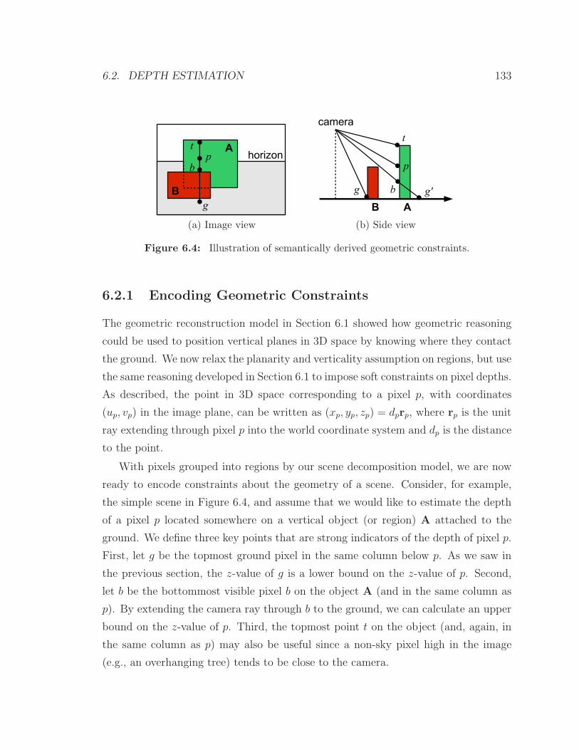
6.2. DEPTH ESTIMATION 133
(a) Image view (b) Side view
Figure 6.4: Illustration of semantically derived geometric constraints.
6.2.1 Encoding Geometric Constraints
The geometric reconstruction model in Section 6.1 showed how geometric reasoning
could be used to position vertical planes in 3D space by knowing where they contact
the ground. We now relax the planarity and verticality assumption on regions, but use
the same reasoning developed in Section 6.1 to impose soft constraints on pixel depths.
As described, the point in 3D space corresponding to a pixel p, with coordinates
(up, vp) in the image plane, can be written as (xp, yp, zp) = dprp, where rp is the unit
ray extending through pixel p into the world coordinate system and dp is the distance
to the point.
With pixels grouped into regions by our scene decomposition model, we are now
ready to encode constraints about the geometry of a scene. Consider, for example,
the simple scene in Figure 6.4, and assume that we would like to estimate the depth
of a pixel p located somewhere on a vertical object (or region) A attached to the
ground. We define three key points that are strong indicators of the depth of pixel p.
First, let g be the topmost ground pixel in the same column below p. As we saw in
the previous section, the z-value of g is a lower bound on the z-value of p. Second,
let b be the bottommost visible pixel b on the object A (and in the same column as
p). By extending the camera ray through b to the ground, we can calculate an upper
bound on the z-value of p. Third, the topmost point t on the object (and, again, in
the same column as p) may also be useful since a non-sky pixel high in the image
(e.g., an overhanging tree) tends to be close to the camera.

134 CHAPTER 6. SCENE RECONSTRUCTION
Simple geometric reasoning allows us to encode the first two constraints as
dg
(
rTg e3
rTp e3
)
≤ dp ≤ dg
(
rTg e2
rTb e2
)(
rTb e3
rTp e3
)
(6.5)
where dp and dg are the distances to the points p and g, respectively, and ei is the
i-th canonical vector (i.e., vector with i-th element one and the rest zero). The point
dg
(r
Tg e2
rTb
e2
)
rb is the point at which the ray through b touches the ground plane, and
is denoted by g′ in Figure 6.4. The third constraint can be similarly encoded as
dtrTt e3 ≈ dpr
Tp e3.
In the following sections we show how these constraints are incorporated as fea-
tures and potential terms in our depth perception MRF model.
6.2.2 Features and Pointwise Depth Estimation
Our goal is to predict the depth to every pixel in the image. We begin by construct-
ing a descriptor fp ∈ Rn for each pixel, which includes local appearance features
and global geometry features derived from our semantic understanding of the scene.
Standard depth perception models utilize the fact that the local appearance of a pixel
changes with depth and attempt to learn a function that describes this relationship.
However, this relationship depends strongly on the semantic class (e.g., a distant tree
will appear less textured than a nearby one, but this is not necessarily so for more
uniform classes such as building or road). Furthermore, the distance of some classes
is tightly constrained by the class itself (e.g., sky). Accordingly, we learn a different
local depth predictor for each semantic class.
Motivated by the desire to more accurately model the depth of nearby objects and
the fact that relative depth is more appropriate for scene understanding, we learn a
model to predict log-depth rather than depth itself. We thus estimate pointwise
log-depth as a linear function of the pixel features (given the pixel’s semantic class),
log dp = θTSpfp (6.6)
where dp is the pointwise estimated depth for pixel p, Sp is its semantic class label

6.2. DEPTH ESTIMATION 135
(a) sky (b) tree (c) road (d) grass
(e) water (f) building (g) mountain (h) foreground obj.
Figure 6.5: Smoothed per-pixel log-depth prior for each semantic class calculated on theMake3d dataset [Saxena et al., 2005]. Images are shifted so that the horizon appears atthe center. Colors indicate distance (red is further away and blue is closer). The classes“water” and “mountain” had very few samples and so are close to the global log-depth prior(not shown).
predicted from our scene decomposition model, fp ∈ Rn is a local feature vector,
and θss∈S are the learned parameters of the model—one parameter vector for each
semantic class label.
Our basic pixel appearance features are the 17 raw filter responses used in the
semantic model and also the log of these features. We also include the (u, v) coor-
dinates of the pixel and an a priori estimated log-depth for a pixel with coordinates
(u, v) and semantic label Sp. These are all adjusted to a consistent coordinate system
(i.e., shifted so that the horizon lies at the center row of the image). The prior log-
depth is learned, for each semantic class, by averaging the log-depth at a particular
(u, v)-pixel location over the set of training images. Since not all semantic class labels
appear at all pixel locations, we smooth the priors with a global log-depth prior (the
average log-depth over all the classes at the particular location). We also enforce
symmetry about the vertical axis by averaging with a mirror-image of the prior.
136 CHAPTER 6. SCENE RECONSTRUCTION
Figure 6.5 illustrates these priors for the eight semantic classes in our model. It is
interesting to note the differences between the semantic classes. A tree pixel towards
the top of the image, for example, is likely to be closer than a tree pixel near the
horizon (center of the image). More important, any pixel within a tree region that
extends towards the top of the image, is likely to be closer than a pixel in a tree
region that does not extend much beyond the horizon. This supports the observation
made in Section 6.2.1 that the location of the topmost pixel in a region may be a
more useful (a priori) indicator for region depth than an arbitrary pixel within the
region.
We encode additional geometric constraints as features by examining the three key
pixels discussed in Section 6.2.1. For each of these pixels (bottommost and topmost
pixel within the same region Rp and topmost ground pixel, all in the same column as
p), we use the pixel’s prior log-depth to calculate a depth estimate for p (assuming
that most objects are roughly vertical) and include this estimate as a feature. We also
include the (horizon-adjusted) vertical coordinate of these pixels as features. Note
that, unlike Section 6.1, our verticality assumption is not a hard constraint, but rather
a soft one that can be overridden by the strength of other features.
As discussed previously, these key pixels are motivated by the observation that
most foreground objects are vertical and therefore pixels on the object within the
same column are likely to be at the same depth. Furthermore, the topmost ground
plane pixel constrains the minimum depth of the object, and a non-sky pixel high in
the image is likely to be closer than one lower in the image. By including these as
features, we allow our model to learn the strength of these a priori constraints.
Finally, we add the square of each feature, allowing us to model quadratic corre-
lations between feature values and depth.
We learn the parameters of the model θss∈S by linear regression on the log-
depths from a set of training images (see Section 2.1). For numerical stability, we
first normalize each feature to zero mean and unit variance. We also include a small
regularization term.

6.2. DEPTH ESTIMATION 137
6.2.3 MRF Model for Depth Reconstruction
The pointwise depth estimation provided by Equation 6.6 is somewhat noisy and can
be improved by including priors that constrain the structure of the scene. We develop
a continuous pixelwise Markov random field (MRF) model to encode such priors. The
priors constrain the depth relationships between two or more pixels, weighted by the
contrast between the pixels to allow for depth discontinuities at strong boundaries.
Our MRF model incorporates terms for encoding three preferences. First, we
would like our predicted depths to be close to the pointwise depth estimates derived
above. Second, we would like to constrain regions to be roughly planar. This amounts
to adding a potential term over three consecutive pixels (in the same row or column)
that prefers co-linearity. Third, we encode semantically-derived depth constraints
which penalize vertical surfaces from deviating from geometrically plausible depths
(as described in Section 6.2.1). Formally, we define the energy function over pixel
depths D as
E (D | I,S) =∑
p
ψp(dp)
︸ ︷︷ ︸
data term
+∑
pqr
ψpqr(dp, dq, dr)
︸ ︷︷ ︸
smoothness
+∑
p
ψpg(dp, dg) +∑
p
ψpb(dp, dg) +∑
p
ψpt(dp, dt)
︸ ︷︷ ︸
geometry (see §6.2.1)
(6.7)
where the data term, ψp, attempts to match the depth for each pixel dp to the
pointwise estimate dp, and ψpqr represents the co-linearity prior. The terms ψpg, ψpb
and ψpt represent the geometry constraints described in Section 6.2.1. Recall that
the pixel indices g, b and t are determined from p and the region to which it belongs,
i.e., they are functions of p.
The data term in our model is given by
ψp(dp) = h(dp − dp;β) (6.8)
where h(x;β) is the Huber penalty, which takes the value x2 for −β ≤ x ≤ β and

138 CHAPTER 6. SCENE RECONSTRUCTION
g g’
ψpg
+ ψpb
Figure 6.6: Graph showing the effect of using the Huber penalty for constraining thedepth range for a pixel p to be between two reference depths g and g′.
β(2|x| − β) otherwise. We choose the Huber penalty because it is more robust to
outliers than the more commonly used ℓ2-penalty and, unlike the robust ℓ1-penalty, is
continuously differentiable (which simplifies inference). In our model, we set β = 10−3.
Our smoothness prior encodes a preference for co-linearity of adjacent pixels within
uniform regions. Assuming pixels p, q, and r are three consecutive pixels (in any row
or column), we have
ψpqr = λsmooth · √γpqγqr · h(2dq − dp − dr;β) (6.9)
where the smoothness penalty is weighted by a contrast-dependent term and the prior
strength λsmooth. Here, γpq = exp (−c−1‖αp − αq‖2) measures the contrast between
two adjacent pixels, where αp and αq are the CIELab color vectors for pixels p and q,
respectively, and c is the mean square-difference over all adjacent pixels in the image.
Note that this is the same pixel-wise contrast term used by the scene decomposition
model of Chapter 4. We choose the prior strength by cross-validation on a set of
training images.
The soft geometry constraints ψpg, ψpt and ψpb model our prior belief that certain

6.3. EXPERIMENTS 139
semantic classes are vertically oriented (e.g., buildings, trees and foreground objects).
Here, we impose the soft constraint that a pixel within such a region should be
the same depth as other pixels above and below it in the region (i.e., by linking to
the topmost and bottommost pixels in the region), and be between the nearest and
farthest ground plane points g and g′ defined in Section 6.2.1. The constraints are
encoded using Huber penalties. For example, the latter constraint can be encoded as
h
(
dp − dg
(
rTg e3
rTp e3
)
;β
)
+ h
(
dp − dg
(
rTg e2
rTb e2
)(
rTb e3
rTp e3
)
;β
)
. (6.10)
Figure 6.6 provides a visualization of this term, clearly showing that the sum of the
two Huber penalties has the desired effect by putting a preference on p lying between
g and g′. In our energy function, we multiply each term by a semantic-specific prior
weight λgs, λ
ts, λ
bss∈S . The final form of each term is
ψpg(dp, dg) = λgSph
(
dp − dg
(
rTg e3
rTp e3
)
;β
)
(6.11)
ψpt(dp, dt) = λtSph
(
dp − dt
(
rTt e3
rTp e3
)
;β
)
(6.12)
ψpb(dp, dg) = λbSph
(
dp − dg
(
rTg e2
rTb e2
)(
rTb e3
rTp e3
)
;β
)
. (6.13)
These weights λgs, λ
ts, λ
bss∈S are learned by cross-validation on the training images.
Our Markov random field formulation in Equation 6.7 defines a convex objective,
which we solve using the L-BFGS algorithm [Nocedal, 1980, Liu and Nocedal, 1989] to
obtain a depth prediction for every pixel in the image. In our experiments, inference
takes about 2 minutes per image (of size 240× 320).
6.3 Experiments
We tested our depth estimation mode by running experiments on the publicly avail-
able Make3d dataset from Saxena et al. [2005]. The dataset consists of 534 images

140 CHAPTER 6. SCENE RECONSTRUCTION
with corresponding depth maps and is divided into 400 training and 134 testing im-
ages. We use Amazon Mechanical Turk (see Chapter 3) to hand-annotate the images
with semantic class labels. The 400 training images were used for learning the pa-
rameters of the semantic and depth models. All images were resized to 240 × 320
before running our algorithm.
We report results on the 134 test images. Since the maximum range of the sensor
used to collect ground truth measurements was 81m, we truncate our depth predic-
tions to the range [0, 81]. Table 6.1 shows our results compared against previous
published results. As is standard on this dataset, we compare both the average log-
error and average relative error, defined as
| log10 gp − log10 dp| and|gp − dp|
gp
, (6.14)
respectively, where gp is the ground truth depth for pixel p. We also compare our
results to our own baseline implementation which does not use any semantic infor-
mation.
Method log10 Rel.
SCN [Saxena et al., 2005]† 0.198 0.530HEH [Hoiem et al., 2005a]† 0.320 1.423Pointwise MRF [Saxena et al., 2008]† 0.149 0.458PP-MRF [Saxena et al., 2008]† 0.187 0.370Baseline (no semantics) 0.208 0.469Pixelwise semantics 0.149 0.375Region-based semantics 0.145 0.372† Results reported in Saxena et al. [2008].
Table 6.1: Quantitative results comparing variants of our “semantic-aware” approach withstrong baselines and other state-of-the-art methods. Baseline models do not use semanticclass information.
We compare three variants of our model. The Baseline variant does not include
any semantic information so provides a measure on how well our raw features predict
depth. The second variant, Pixelwise semantics, includes semantic information,
but not region information. As discussed above, this model derives region boundaries
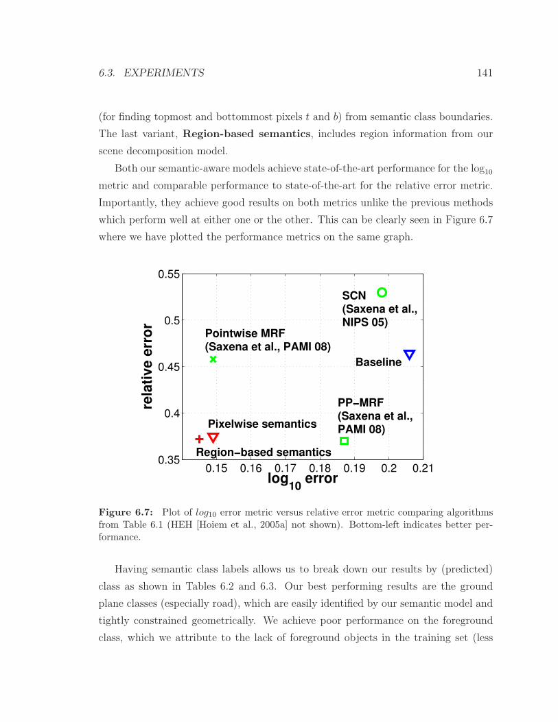
6.3. EXPERIMENTS 141
(for finding topmost and bottommost pixels t and b) from semantic class boundaries.
The last variant, Region-based semantics, includes region information from our
scene decomposition model.
Both our semantic-aware models achieve state-of-the-art performance for the log10
metric and comparable performance to state-of-the-art for the relative error metric.
Importantly, they achieve good results on both metrics unlike the previous methods
which perform well at either one or the other. This can be clearly seen in Figure 6.7
where we have plotted the performance metrics on the same graph.
0.15 0.16 0.17 0.18 0.19 0.2 0.210.35
0.4
0.45
0.5
0.55
log10
error
rela
tiv
e e
rro
r
SCN(Saxena et al.,NIPS 05)
Baseline
Pointwise MRF(Saxena et al., PAMI 08)
PP−MRF(Saxena et al.,PAMI 08)
Region−based semantics
Pixelwise semantics
Figure 6.7: Plot of log10 error metric versus relative error metric comparing algorithmsfrom Table 6.1 (HEH [Hoiem et al., 2005a] not shown). Bottom-left indicates better per-formance.
Having semantic class labels allows us to break down our results by (predicted)
class as shown in Tables 6.2 and 6.3. Our best performing results are the ground
plane classes (especially road), which are easily identified by our semantic model and
tightly constrained geometrically. We achieve poor performance on the foreground
class, which we attribute to the lack of foreground objects in the training set (less

142 CHAPTER 6. SCENE RECONSTRUCTION
log10 Error
All Pixels Correct Incorrect Baseline
Sky 0.155 0.118 0.304 0.434Tree 0.207 0.208 0.197 0.232Road 0.058 0.052 0.141 0.079Grass 0.098 0.084 0.140 0.139Water 0.089 - 0.089 0.167Building 0.189 0.178 0.241 0.288Mountain 0.353 - 0.353 0.270Foreground 0.223 0.318 0.209 0.245All Classes 0.145 0.133 0.207 0.208
Table 6.2: Quantitative results by predicted semantic class (log10 error).
Relative Error
All Pixels Correct Incorrect Baseline
Sky 0.612 0.492 1.095 0.678Tree 0.504 0.517 0.423 0.587Road 0.132 0.111 0.402 0.202Grass 0.233 0.198 0.337 0.273Water 0.222 - 0.222 0.473Building 0.442 0.360 0.826 0.665Mountain 0.860 - 0.860 0.387Foreground 0.584 1.657 0.424 0.609All Classes 0.372 0.334 0.567 0.469
Table 6.3: Quantitative results by predicted semantic class (relative error).
than 1% of the pixels). Likewise, the small number of water and mountain pixels
limit the conclusions we can draw from these classes.
Unexpectedly, we also perform poorly on sky pixels which are easy to predict and
should always be positioned at the maximum depth. This is due, in part, to errors in
the ground truth measurements (caused by sensor misalignment) and the occasional
misclassification of the reflective surfaces of buildings as sky by our semantic model.
Note that the nature of the relative error metric is to magnify these mistakes since the
ground truth measurement in these cases is always closer than the maximum depth.
Given our heavy reliance on inferred semantic evidence at the depth estimation
stage, it is also important to consider the robustness of our approach to errors in
6.4. CHAPTER SUMMARY 143
the semantic labeling. Quantitatively, about 16% of pixels were classified with the
wrong semantic class. Tables 6.2 and 6.3 include results calculated on the subset
of pixels that were either correctly or incorrectly classified. As expected, the depth
estimation accuracy is better on correctly classified pixels than those misclassified.
Surprisingly, the depth estimation accuracy over the incorrect pixels was comparable
to the baseline model (0.207 versus 0.208 for log10 error and 0.567 versus 0.469 for
relative error) showing that the depth-estimation stage of our approach is able to
partially overcome mistakes made in the semantic classification stage.
Finally, we show some qualitative results in Figure 6.8 and example 3D recon-
structions in Figure 6.9. The results show that we correctly model co-planarity of the
ground plane and building surfaces. Notice our accurate prediction of the sky (which
is sometimes penalized by misalignment in the ground truth, e.g., the example in the
bottom row). Our algorithm also makes mistakes, such as positioning the building
too close in the second row and missing the ledge in the foreground (a mistake that
many humans would also make). We also miss some low contrast objects such as the
post in the example at the top of the figure. However, in general, we produce very
accurate results.
6.4 Chapter Summary
In this chapter we presented two models for 3D reconstruction of the scene. Both
models make heavy use of predicted semantic information. The first model used
basic geometric reasoning over the region output of our scene decomposition model
to produce 3D “pop ups” of the scene. The second model predicts real-world depths
guided by the semantic labels for each pixel. The inclusion of semantic information
allowed us to model appearance and geometry constraints that were not possible in
previous works (e.g., [Saxena et al., 2008]).
Our depth estimation models did not make use of refined foreground object infor-
mation which, as other researchers have also noted [Saxena et al., 2008, Hoiem et al.,
2007a], could provide strong constraints on 3D distances. For example, knowing the
distribution over object sizes (in a particular category, say, people), puts a constraint
144 CHAPTER 6. SCENE RECONSTRUCTION
on distances within the scene. Unfortunately, the lack of ground truth training data
containing foreground objects complicates their inclusion into the model. We note
that Saxena et al. [2008] demonstrates the use of detected objects for encoding (ver-
tical) orientation priors, much like our use of foreground semantics. However, they
do not make use of object size.
A possible solution is to use manufacturer’s specifications (or anatomical statis-
tics, in the case of animals) to estimate distributions over object sizes. These could
then be encoded as soft constraints in the model like many of our other terms. It
remains to be able to learn the relative strength of these terms which will depend on
their interactions with other energy terms and on the quality of the object detectors.
Weakly supervised data containing foreground objects, and with a few pairwise dis-
tances hand-annotated (per image) may be sufficient for this purpose. Alternatively,
synthetic data (e.g., extracting ground truth depth from ray-traced scenes) may be
employed, or a combination of synthetic and weakly labeled images used. These
approaches present interesting directions for future work.
Objects can be used in other ways, too. Our depth estimation model (and those
in previous works) make a strong assumption about the focal length of the camera,
which is necessary for computing the orientation of rays rp extending through the
camera plane into the scene. A natural extension, of this work, is to remove this
assumption and infer the focal length from features in the image. One possibility
is to make use of foreground objects for this purpose. However, purely scaling for
the height of an object is not sufficient, since there remains a scaling ambiguity that
object height alone does not address: Is the object twice as large because it is half the
distance to the camera, or because the camera has half the focal length? To answer
this question, an algorithm would need to extract z-value distances, for example,
between objects (or landmarks) at different depths, in addition to object width and
height parallel to the imaging plane.
Finally, this chapter has addressed the problem of using predicted semantic infor-
mation to guide 3D reconstruction as a two-stage process. An interesting question,
partially addressed in Chapter 4 and also in some other works on holistic scene un-
derstanding (e.g., [Heitz et al., 2008b]), is whether we can go in the other direction.

6.4. CHAPTER SUMMARY 145
That is, how can we use 3D constraints and, in particular, depth estimates derived
from image features to guide semantic understanding? One of the most compelling
directions for future research, as we shall discuss in Chapter 7, is the joint inference
over these aspects of the scene in a single unified model.

146 CHAPTER 6. SCENE RECONSTRUCTION
Figure 6.8: Qualitative depth estimation results on the Make3d dataset [Saxena et al.,2005]. Shown (from left to right) are the image, semantic overlay, ground truth depthmeasurements, and our predicted depth estimates. The legends shows semantic color labelsand depth scale.

6.4. CHAPTER SUMMARY 147
Figure 6.9: Novel 3D views of different scenes generated from our semantically-awaredepth reconstruction model.

148 CHAPTER 6. SCENE RECONSTRUCTION
Chapter 7
Conclusions and Future Directions
Our work has focused on understanding three main aspects of a scene—regions, ob-
jects, and geometry. We have done so using a holistic model that enforces consistency
and allows information to propagate between these different aspects of a scene. In
this final chapter, we summarize our model and discuss its contributions. We then
present some open problems and challenges for future research.
7.1 Summary
In this dissertation, we tackled the problem of holistic scene understanding. We pre-
sented a unified model for understanding scenes in terms of their dominant regions,
objects, and geometry. These three aspects of the scene are key to higher-level in-
terpretation. The most important feature of our model is that it is holistic. That is,
we jointly reason over the three scene aspects rather than treat them as independent
tasks. This enforces consistency in our representation and hence interpretation of the
scene. In addition, the introduction of regions as variables in our model means that
we are not committing to early bottom-up segmentation decisions that may result in
degraded performance.
In Chapter 4 we introduced the first components of our model for decomposing
a scene into semantic and geometrically consistent regions. Entities in the scene
(pixels, regions and geometry) were encoded as random variables in a conditional
149

150 CHAPTER 7. CONCLUSIONS AND FUTURE DIRECTIONS
Markov random field (CRF) model, which allows for preferences of assignments to
subsets of variables to be specified. We showed how these preferences could be learned
from labeled training data. Exact inference in our model is intractable so we proposed
a move-making approach that performs very well in practice.
When decomposing the scene into regions, we focused on a number of background
classes that are typically found in outdoor scenes. These were easily characterized
by local color and texture information. We also included a (single) foreground object
class label. Foreground objects are harder to characterize in terms of local features and
we found that many objects, while separated from the background, were themselves
segmented into multiple regions. For example, people tended to be divided into head,
torso, and legs, and cars into wheels and body.
We extended our model in Chapter 5 to incorporate the notion of objects. This
involved the refinement of (one or more) foreground regions into specific object cate-
gories. Random variables representing objects and their corresponding energy terms
were introduced into the model. The energy terms scored how likely a proposed
object was to be one of the known object categories. Other energy terms encoded
contextual preferences between objects and their neighboring regions (e.g., cars are
found on roads; boats are found on water). An important benefit of our holistic model
was that we were able to provide a precise (pixel-level) boundary for objects rather
than the standard bounding box representation. However, we were still able to take
advantage of strengths of bounding box approaches in proposing top-down moves that
suggested candidate locations for objects. Each move was then evaluated against our
unified energy function ensuring that we were optimizing a consistent objective.
In the final technical chapter, Chapter 6, we showed how simple geometric rea-
soning applied to our region-based decomposition of a scene could lead to plausible
3D planar reconstructions. Building on this geometric reasoning, we then developed
a continuous CRF model that incorporated semantic labels and region boundary in-
formation to guide depth prediction in outdoor scenes. This model outperformed
current state-of-the-art approaches on the task of depth estimation from monocular
images.

7.2. OPEN PROBLEMS AND FUTURE DIRECTIONS 151
7.2 Open Problems and Future Directions
Our work has made some progress towards the long-term goal of scene understanding.
However, there are still many questions left unanswered and plenty more work to be
done. This section discusses some of the limitations of our current approach and
suggests a number of possible directions for building on our work.
7.2.1 Learning from Multiple Sources
As discussed in Chapter 3, the availability of high-quality datasets in computer vision
is becoming more prevalent. However, there are still a significant number of object
categories and scene types that are not represented in existing datasets. Furthermore,
for some computer vision tasks, data is still difficult to collect. For example, one of
the limitations of the depth estimation model was that it required image-aligned
ground truth depth measurements for training. This is difficult to acquire, especially
for distant and moving objects.
In addition, many existing datasets are labeled for a specific task in mind. In order
to leverage these valuable resources (as opposed to relabeling all the images every time
we wish to consider a new task), it will be beneficial to develop approaches that can
learn from multiple disjoint sources. Our existing framework does this to a limited
extent. For example, the object detectors are learned from a separate set of cropped
images and later integrated into the larger scene model. However, a more integrated
approach that allows disjoint training sources at all levels of the algorithm is still
needed.
An exciting direction for future work that addresses these limitations is to extend
our framework to make use of large corpora of partially labeled data, synthetic train-
ing data, and video sequences. This has the potential to fill the gap and provide depth
information (e.g., from ray-traced synthetic scenes) and segmentation cues (e.g., by
extracting motion cues from video). As discussed in previous chapters, the use of
max-margin learning algorithms for structured prediction are a promising direction
for training our models, and extensions that allow for latent variables (e.g., [Yu and
Joachims, 2009]) make training with partially labeled data feasible.

152 CHAPTER 7. CONCLUSIONS AND FUTURE DIRECTIONS
7.2.2 Structure and Occlusion
Our current work has focused on understanding images of outdoor scenes, in par-
ticular, urban, rural and harbor. However, there are many other scenes types with
markedly different geometric structure that we would like to understand. For exam-
ple, indoor scenes present a very different challenge to outdoor scenes.
Even more interesting are scenes with considerably different scales. For example,
understanding the difference between a close-up of a person’s face or a zoomed-in view
of some workspace versus an entire urban landscape. Our current model makes strong
assumptions about the scene structure, and in these scenarios those assumptions are
clearly violated. Instead of relying on global geometry, understanding close-up images
requires local geometric reasoning similar to the early work of inferring geometry from
line drawings [Waltz, 1975] or structure from shading [Horn, 1989].
Other than scale, one of the most important cues that we can derive from scene
structure is knowing the relative location of objects and thus be able to reason about
occlusion. Presently, occlusion reasoning is absent from our model. An interesting
research direction is in developing models that make better use of our geometric un-
derstanding of a scene to determine what parts of an object (candidate) are occluded
and taking that information into account. For example, if a person is standing be-
hind a car so that their legs are occluded, then the object term in our energy function
should not look for visual evidence of legs. Likewise, if we have no evidence that an
object is occluded, then the object term should penalize missing features.
Occlusion modeling can be extended to take into account transparent objects
(which would require allowing a pixel to be associated with two different objects).
For example, a person looking out of a glass window. This becomes important when
we start trying to understand the activities in a scene, as we discuss below. For
example, the question “is there a person inside the car?” can only be answered if we
can see a person through the car’s windows or windshield.
Finally, as discussed in Chapter 6, our current model performs depth estimation
after decomposing the scene into regions. While we were able to produce state-of-
the-art results for depth estimation, it did not allow us to make use of this depth
information when decomposing the scene or identifying objects (other than implicit

7.2. OPEN PROBLEMS AND FUTURE DIRECTIONS 153
cues from the location of the horizon and region configuration). Developing a model
that jointly optimizes over depth prediction and scene decomposition poses significant
challenges, but would allow stronger coupling between these aspects of the scene.
7.2.3 Expanding the Object Classes
Our approach currently only recognizes objects from a small set of categories. The
region layer handles this by allowing regions to be annotated with a generic foreground
object class label. However, at the object layer we would like to be able to identify
many thousands of object types. Scaling to this magnitude is a significant challenge
in many respects. First, we would need to collect labeled training instances for
each object class. Second, the object energy term would now have many competing
hypotheses (due to the increased label space). Intuitively, this increases the chance of
false positives. Last, as the number of object classes increases, the similarity between
object categories complicates training and evaluation. For example, is mistaking a
car for a truck as bad an error as mistaking a car for a horse?
Regarding the first challenge, an important limitation of our current approach
is its reliance on a large amount of hand-labeled training data. As discussed in
Section 7.2.1 above, extending our framework to make use of diverse data sets is a
viable solution to this problem.
An interesting direction for addressing the second challenge is to develop model-
free methods for object labeling within a higher-level model of scene structure. For
example, object candidates can be matched to a large dictionary of labeled samples.
The matched instances then need to be coherently placed within the scene using the
region and geometry aspects of the model. An advantage of this approach is that it
is an open universe allowing new object instances and categories to be incrementally
added without changing the underlying model. It also presents exciting opportunities
for active learning paradigms and object discovery.
The last challenge gets at the heart of the scene understanding problem. As
discussed in the introduction, the real goal is to enable autonomous agents to interpret
scenes so as to provide a description, answer questions, or perform some action. Thus,

154 CHAPTER 7. CONCLUSIONS AND FUTURE DIRECTIONS
it is the final application that determines the quality of the scene understanding
framework. For example, a safety system in an autonomous vehicle need not worry
about confusing a car with a horse, so long as it avoids an accident. Alternatively, a
content retrieval system may wish to have high precision so that when a user searches
for images of horses, the system does not return cars. The next two sections deal
with two different subtleties raised by this challenge.
7.2.4 Hierarchical Decomposition
Currently, our model decomposes a scene over a very shallow hierarchy. We associate
pixels to regions, and regions to objects. However, many objects that we are interested
in are made up of different parts (such as the wheels of a car), which are not captured
in our model. Decomposing the scene over a deeper hierarchy, also known as image
parsing will present three key advantages.
First, in describing or answering questions about a scene, we may need to know
about object parts and poses (e.g., answering the question “does the car have a flat
tire?” requires that know how to decompose a car into parts, and what a flat tire looks
like independent of the general appearance of cars). As we discuss in the following
section, this can be achieved if we already have a hierarchical decomposition rather
than as a post-processing step where the relevant information may not be readily
available.
The second benefit of a hierarchical decomposition is that it addresses some of
the issues raised above in expanding the set of recognizable object categories. For
example, learning models of common parts and attributes, and sharing these learned
models between objects may allow us to learn better object models (especially when
training data is scarce).
Last, the hierarchical approach may present some opportunities for accelerating
inference when the number of object categories grows large. For example, by elim-
inating unlikely object hypotheses while building up our understanding of a scene
(e.g., all objects that do not have wheels), the value space of object variables can be
significantly pruned.

7.3. CONCLUSION 155
7.2.5 Activity Recognition
In claiming to have understood a scene, we have developed a model that can recognize
objects, annotate background regions, and reconstruct coarse geometry. However,
this is not enough to really be able to describe what the scene is about. Complete
scene understanding also requires the ability to reason about the activities that are
happening within the scene. This opens up a whole new thrust of research into how
to make use of our region-based understanding to infer the actions behind the scene.
We expect that by building on our decomposition of the scene into regions and
object, many activities can be readily identified by making use of the 3D relationships
between interacting objects and their parts. As discussed above, this requires a
hierarchical decomposition so the we can identify relevant parts. For example, a
person kneeling down next to the wheel of a car is possibly changing a flat tire, and
a cow with its head down next to a trough is probably drinking water.
7.3 Conclusion
This thesis has explored the problem of holistic scene understanding by integrating
the tasks of segmentation, multi-class image labeling, object detection, and depth
reconstruction into a single unified model. However, as discussed in the previous
section, there is still much work to be done on improving these methods and exciting
directions in which they can be extended. We hope that our work can provide the
foundations on which further research can stand.

156 CHAPTER 7. CONCLUSIONS AND FUTURE DIRECTIONS

Appendix A
Implementation Details
Inference in our region-based models, as discussed in Chapter 4 and Chapter 5, in-
volves repeated execution of two expensive operations—computing region features and
checking for connectedness of the regions. Specifically, every time a proposal move
is made it changes the pixel-to-region associations and these two operations must be
performed. They become the computational bottleneck during inference, so to achieve
good runtime performance they need to be optimized. In this section we present some
implementation details that describe the data structures and algorithms that enable
fast execution of region feature calculation and connected component finding.
We will assume that the inference algorithm is running on a W -by-H image I. A
pixel p ∈ I is indexed by its (u, v) coordinates in the image plane, with u ∈ 1, . . . ,Wand v ∈ 1, . . . , H, and we store our pixel-to-region association variables in an integer
matrix R ∈ ZH×W so that Rvu indicates the region to which pixel (u, v) belongs.1
The set of pixels belonging to region r is then Pr = (u, v) | Rvu = r. Likewise, we
will assume that any feature computed at the pixel level, specifically, the αp’s, are
arranged in feature matrices F (1), . . . , F (n) ∈ RH×W where the element F
(i)vu stores the
i-th component of feature vector αp for pixel (u, v).2 This is illustrated in Figure A.1.
1Note that matrices are indexed in row-major order, i.e., the v coordinate first and the u coor-dinate second. To avoid confusion in dealing with image indexing and matrix indexing, we will useparentheses for column-major indexing and subscripts for row-major indexing, so that Rvu = R(u, v).
2Arranging the storage of these matrices so that F(1)vu , . . . , F
(n)vu are contiguous in memory will
result in better cache locality and thus faster execution.
157
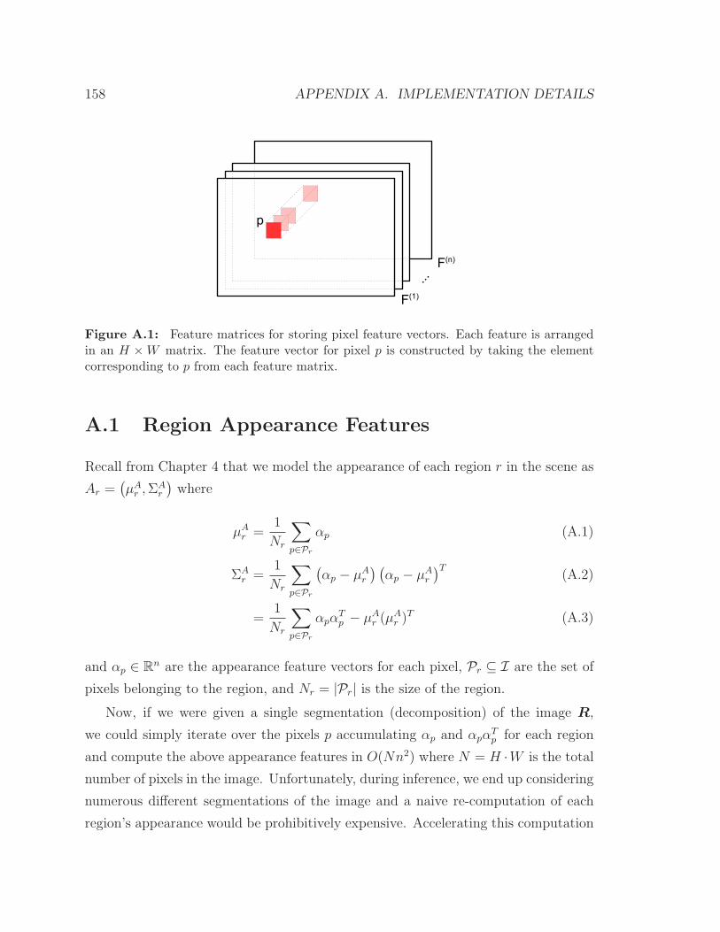
158 APPENDIX A. IMPLEMENTATION DETAILS
Figure A.1: Feature matrices for storing pixel feature vectors. Each feature is arrangedin an H ×W matrix. The feature vector for pixel p is constructed by taking the elementcorresponding to p from each feature matrix.
A.1 Region Appearance Features
Recall from Chapter 4 that we model the appearance of each region r in the scene as
Ar =(µA
r ,ΣAr
)where
µAr =
1
Nr
∑
p∈Pr
αp (A.1)
ΣAr =
1
Nr
∑
p∈Pr
(αp − µA
r
) (αp − µA
r
)T(A.2)
=1
Nr
∑
p∈Pr
αpαTp − µA
r (µAr )T (A.3)
and αp ∈ Rn are the appearance feature vectors for each pixel, Pr ⊆ I are the set of
pixels belonging to the region, and Nr = |Pr| is the size of the region.
Now, if we were given a single segmentation (decomposition) of the image R,
we could simply iterate over the pixels p accumulating αp and αpαTp for each region
and compute the above appearance features in O(Nn2) where N = H ·W is the total
number of pixels in the image. Unfortunately, during inference, we end up considering
numerous different segmentations of the image and a naive re-computation of each
region’s appearance would be prohibitively expensive. Accelerating this computation

A.1. REGION APPEARANCE FEATURES 159
warrants some upfront work to organize the feature values in a more convenient form.
As we shall see, one such convenient form is to precompute integrals along each row
of the feature matrix. However, before describing these row integrals we begin by
discussing the more familiar integral images.
Integral images were first introduced by Crow [1984] and now used extensively in
computer vision. The integral image for a feature matrix F (i), which we denote by
F(i)int is an (H + 1)× (W + 1) matrix whose (u, v)-th entry contains the the sum of all
entries in F (i) above and to the left of pixel (u, v), i.e.,
F(i)int (u, v) =
∑
u′<u,v′<v
F (i)(u′, v′). (A.4)
The integral image can be computed in a single pass through the feature matrix, and
once computed can be used to find the sum of feature values within any rectangular
region in the image in constant time. Consider, for example, the rectangle ABCD
in Figure A.2(a). It is straightforward to see that the sum of features within this
rectangle can be calculated as
∑
uA≤u<uDvA≤v<vD
F (i)(u, v) = F(i)int (uA, vA) + F
(i)int (uD, vD)− F (i)
int (uB, vB)− F (i)int (uC , vC). (A.5)
The idea of integral images can be readily extended to squared integral images for
computing the sum over features squared, and even adapted to compute integrals
over rectangular regions rotated by 45.
Unfortunately, for non-rectangular regions, integral images fail to be beneficial.
For arbitrary shaped regions some work has been done in extending Green’s Theorem
(which relates the double integral over a closed surface to the line integral around its
contour) to the discrete domain [Tang, 1982, Yang and Albregtsen, 1996]. However,
these approaches require the boundary of each region to be traversed (and therefore
computed and stored explicitly). We elect to use a simpler approach that shares ideas
developed in Kumar et al. [2004] for accelerating similar computations in their work.
Our approach has the added advantage of being applicable to the case of computing

160 APPENDIX A. IMPLEMENTATION DETAILS
(a) Integral image (b) Row integral
Figure A.2: Integral images and row integrals. Integral images are useful for efficientlycomputing the sum of feature values within a rectangular region, but fail to be of use onarbitrary shaped regions.
features over all regions in the image in a single pass.
We define the row integral F(i)r-int to be an H × (W + 1) matrix whose (u, v)-th
entry contains the the sum of all entries in F (i) to the left of pixel (u, v), i.e.,
F(i)r-int(u, v) =
∑
u′<u
F (i)(u′, v). (A.6)
Like the integral image, the row integrals can be computed in a single pass through
the feature matrix. Similarly, we can define the squared row integral as
F(i,j)sq-r-int(u, v) =
∑
u′<u
F (i)(u′, v) · F (j)(u′, v). (A.7)
With these row integrals precomputed, we can now compute the region appearance
features in O(N+Bn2) time using Algorithm A.1. Here B is the number of boundary
pixels (transitions) between regions.3 Note that usually we have B ≪ N . In addition,
the algorithm can be modified to include an explicit check for the special-case of single
pixel transitions and resort to using the feature matrices directly in this case (saving
3The boundary pixels include pixels at the left and right image boundaries. In cases where regionsare likely to wrap around the edge of the image (e.g., a large contiguous sky region), a raster scan
integral as opposed to row integrals may provide additional speedup.
A.2. CHECKING FOR CONNECTED COMPONENTS 161
an overhead of n2 + n operations).
The computational gains can be understood by considering the example region in
Figure A.2(b). For the line indicated, a naive approach would require summing over
all shaded pixels. However, using our integral rows we can compute the sum over the
two connected shaded area using four operations (per feature value), e.g.,
F(i)r-int(uB, v)− F (i)
r-int(uA, v) + F(i)r-int(uD, v)− F (i)
r-int(uC , v) (A.8)
for the i-th feature. Note that in Algorithm A.1 we use the notation(
F(i)r-int(u, v)
)n
i=1
and(
F(i)sq-r-int(u, v)
)n
i=1,jto represent the n-vector and n× n matrix formed by taking
the corresponding entries of F(i)r-int(u, v) and F
(i,j)sq-r-int(u, v), respectively.
While the algorithm has been described for calculating the aggregate features
for an entire image, we can further improve performance by maintaining sufficient
statistics over each region. Then whenever a move is proposed, we only need to adjust
the sufficient statistics by iterating over the modified pixels, resulting in dramatically
faster computation.
A.2 Checking for Connected Components
In Chapter 4 we noted that currently, our method for scene decomposition requires
that the regions be connected components. We now make precise our definition of
connected component and describe an algorithm which efficiently checks for connect-
edness. We begin by defining the neighborhood of a pixel:
Definition A.2.1: The neighborhood of pixel p is a set of pixels N (p) is such that
p /∈ N (p) and if pixel q ∈ N (p) then p ∈ N (q). We will use N (P) to denote the
neighborhood of a set of pixels P , i.e., N (P) =⋃
p∈P N (p).
Of interest to us will be 4-connected and 8-connected neighborhoods. These are
illustrated in Figure A.3 and formalized by the following definitions:
Definition A.2.2: The 4-connected neighborhood of pixel p = (u, v) is the set of
pixels N4(p) = (u− 1, v), (u, v − 1), (u, v + 1), (u+ 1, v). Similarly, the 8-connected

162 APPENDIX A. IMPLEMENTATION DETAILS
(a) 4-connected neighborhood (b) 8-connected neighborhood
Figure A.3: 4-connected and 8-connected neighborhoods.
neighborhood of pixel p = (u, v) is the set of pixels N8(p) = (u − 1, v − 1), (u −1, v), (u− 1, v + 1), (u, v − 1), (u, v + 1), (u+ 1, v − 1), (u+ 1, v), (u+ 1, v + 1).
We are now ready to define a connected component. Recall that a region r contains
the set of pixels Pr. The following definition encapsulates what it means for region r
to be connected.
Definition A.2.3: Two pixels p and q, both in region r, are connected with respect
to some neighborhood N if there exists a set of pixels i1, . . . , in ⊆ Pr such that
i1 = p, in = q, and for all k < n, ik ∈ N (ik+1). Region r is a connected component if
∀(p, q) ∈ Pr ×Pr, p and q are connected.
The most naive approach to determining whether a region is connected or not is
to perform a breadth-first or depth-first search over neighboring pixels. Specifically,
starting from any pixel p ∈ Pr we place all neighbors q ∈ N (p) ∩ Pr into a queue.
Then, while the queue is not empty, we pop an element p′ from the queue and, if p′
has not been visited previously, add all of its neighbors q′ ∈ N (p′)∩Pr to the queue.
The set of visited pixels forms a connected component, and if all pixels in Pr were
visited, then the region is a connected. If the region is not connected, then we can
break it into connected components, by iteratively finding a pixel in the region that
has not yet been visited and applying the above algorithm.
While the above approach to finding connected components is linear in the size of
the image, it suffers from needing to maintain a queue data structure and having to

A.2. CHECKING FOR CONNECTED COMPONENTS 163
examine the entire neighborhood of each pixel. Instead of this approach, we propose
a method that groups connected components along rows in the image and makes
use of a disjoint sets (or union-find) data structure [Cormen et al., 2001] to merge
connected groups. Other researchers (e.g., [Strandh and Lapeyre, 2004]) have found
performance gains using similar approaches.
Our method is presented in Algorithm A.2. Briefly, we iterate through the image
from top-left to bottom-right maintaining disjoint sets of pixels. At each pixel p, we
examine the pixel’s region-association variable Rp to determine whether it belongs to
the same region as the previous pixel in the same row. If so, we add the pixel to the
same set as the previous pixel. Otherwise, we start a new set P = p. In addition
to maintaining the set of (sets of) pixels, we also maintain a list of edges between
neighboring sets. Again, at each pixel p, we examine the pixels in the row above (that
are also within the pixel’s neighborhood). For each of these pixels q, if q belongs to
the same region as p we add edge between the set containing p and the set containing
q. Finally (in Line 25 of Algorithm A.2), we merge all pixel sets with an edge between
them (using union and find operations on the disjoint sets data structure [Cormen
et al., 2001]).
The above algorithm, in addition to not having to search the full neighborhood of
each pixel (since we only ever examine the pixel to the left and the row above), allows
us to re-use calculations when proposing moves. Like the algorithm for computing
region appearance, by caching the connected row segments V and the neighborhood
set E (and some housekeeping data), Algorithm A.2 can be modified to operate on
the set of pixels modified by a move resulting significant performance gains.
We have presented the algorithms for updating region appearance and finding
connected components as two separate stages. However, the astute reader will have
noticed that both algorithms iterate through the image performing operations on con-
nected row segments. By maintaining a data structure over connected row segments,
we can iterate over modified pixels once and perform both computations quickly.

164 APPENDIX A. IMPLEMENTATION DETAILS
Algorithm A.1: Compute Region Features.
Input : R // region association variables1
F (i)r-intni=1 // row integrals2
F (i,j)sq-r-intni,j=1 // squared row integrals3
Output: A // region appearance variables4
initialize Nr = 0, µAr = 0n×1 and ΣA
r = 0n×n for each region r5
for v = 1, . . . , H do6
set s = R(u, v)7
for u = 1, . . . ,W do8
set r = R(u, v)9
Nr ← Nr + 110
if r 6= s then11
µAr ← µA
r −(
F(i)r-int(u, v)
)n
i=1and ΣA
r ← ΣAr −
(
F(i,j)sq-r-int(u, v)
)n
i,j=112
µAs ← µA
s +(
F(i)r-int(u, v)
)n
i=1and ΣA
s ← ΣAs +
(
F(i,j)sq-r-int(u, v)
)n
i,j=113
s← r14
end15
end16
µAs ← µA
s +(F (i)(W + 1, v)
)n
i=1and ΣA
s ← ΣAs +
(
F(i,j)sq-r-int(W + 1, v)
)n
i,j=117
end18
foreach region r do19
set µAr ← 1
NrµA
r20
set ΣAr ← 1
NrΣA
r − µAr (µA
r )T21
end foreach22
return Ar = (µAr ,Σ
Ar )23

A.2. CHECKING FOR CONNECTED COMPONENTS 165
Algorithm A.2: Find Connected Components.
Input : R // region association variables1
N // neighborhood operator (e.g., N4 or N8)2
Output: C // set of connected components3
initialize V = ∅ and E = ∅4
for v = 1, . . . , H do5
initialize active pixel set P to (1, v)6
for u = 2, . . . ,W do7
if R(u, v) = R(u− 1, v) then8
P ← P ∪ (u, v)9
end10
if R(u, v) 6= R(u− 1, v) or u = W then11
add to P to V12
foreach (u′, v′) ∈ N (P) such that v′ = v − 1 do13
if R(u′, v′) = R(u− 1, v) then14
let P ′ be the pixel set containing (u′, v′)15
add edge (P ,P ′) to E16
end17
end foreach18
if u 6= W then19
re-initialize active pixel set P = (u, v)20
end21
end22
end23
end24
C = union(V, E)25
return C26

166 APPENDIX A. IMPLEMENTATION DETAILS

Bibliography
H. Barrow and J. Tenenbaum. Computational vision. Proc. of the IEEE, pages
572–295, 1981.
J. Besag. Statistical analysis of non-lattice data. The Statistician, pages 179–195,
1975.
J. Besag. On the statistical analysis of dirty pictures. Journal of the Royal Statistical
Society Series B, 48:259–302, 1986.
S. Bileschi and L. Wolf. A unified system for object detection, texture recognition,
and context analysis based on the standard model feature set. In Proc. of the
British Machine Vision Conference (BMVC), 2005.
C. M. Bishop. Neural Networks for Pattern Recognition. Oxford University Press,
1996.
C. M. Bishop. Pattern Recognition and Machine Learning. Springer, 2007.
E. Borenstein and S. Ullman. Class-specific, top-down segmentation. In Proc. of the
European Conference on Computer Vision (ECCV), 2002.
S. P. Boyd and L. Vandenberghe. Convex Optimization. Cambridge, 2004.
Y. Boykov, O. Veksler, and R. Zabih. Fast approximate energy minimization via
graph cuts. In Proc. of the International Conference on Computer Vision (ICCV),
1999.
167
168 BIBLIOGRAPHY
Y. Y. Boykov and M.-P. Jolly. Interactive graph cuts for optimal boundary and region
segmentation of objects in n-d images. In Proc. of the International Conference on
Computer Vision (ICCV), 2001.
R. Brooks. Model-based 3-D interpretations of 2-D images. IEEE Trans. on Pattern
Analysis and Machine Intelligence (PAMI), pages 140–150, 1983.
S. C. Brubaker, J. Wu, J. Sun, M. D. Mullin, and J. M. Rehg. On the design of
cascades of boosted ensembles for face detection. International Journal of Computer
Vision (IJCV), 2007.
J. Canny. A computational approach to edge detection. IEEE Trans. on Pattern
Analysis and Machine Intelligence (PAMI), pages 679–714, 1986.
D. Comaniciu and P. Meer. Mean shift: A robust approach toward feature space
analysis. IEEE Trans. on Pattern Analysis and Machine Intelligence (PAMI), 24:
603–619, 2002.
T. H. Cormen, C. E. Leiserson, R. L. Rivest, and C. Stein. Introduction to Algorithms.
MIT Press and McGraw-Hill, 2001.
A. Criminisi. Microsoft research cambridge (MSRC) object recogni-
tion image database (version 2.0), 2004. Available for download from
http://research.microsoft.com/vision/cambridge/recognition.
A. Criminisi, I. Reid, and A. Zisserman. Single view metrology. International Journal
of Computer Vision (IJCV), 2000.
F. Crow. Summed-area tables for texture mapping. In Proc. of the International
Conference on Computer Graphics and Interactive Techniques (SIGGRAPH), pages
207–212, 1984.
N. Dalal and B. Triggs. Histograms of oriented gradients for human detection.
In Proc. of the IEEE Conference of Computer Vision and Pattern Recognition
(CVPR), 2005.

BIBLIOGRAPHY 169
E. Delage, H. Lee, and A. Y. Ng. A dynamic Bayesian network model for autonomous
3D reconstruction from a single indoor image. In Proc. of the IEEE Conference on
Computer Vision and Pattern Recognition (CVPR), 2006.
J. Deng, W. Dong, R. Socher, L.-J. Li, K. Li, and L. Fei-Fei. ImageNet: A large-scale
hierarchical image database. In Proc. of the IEEE Conference on Computer Vision
and Pattern Recognition (CVPR), 2009.
S. K. Divvala, D. Hoiem, J. H. Hays, A. A. Efros, and M. Hebert. An empirical study
of context in object detection. In Proc. of the IEEE Conference on Computer
Vision and Pattern Recognition (CVPR), 2009.
R. O. Duda, P. E. Hart, and D. G. Stork. Pattern Classification. Wiley-Interscience,
2000.
G. Elidan, I. McGraw, and D. Koller. Residual belief propagation: Informed schedul-
ing for asynchronous message passing. In Proc. of the Uncertainty in Artificial
Intelligence (UAI), 2006.
M. Everingham, L. Van Gool, C. K. I. Williams, J. Winn, and A. Zisserman. The
PASCAL Visual Object Classes Challenge 2010 (VOC2010) Results, 2010.
L. Fei-Fei, R. Fergus, and P. Perona. Learning generative visual models from few train-
ing examples: an incremental Bayesian approach tested on 101 object categories.
In Proc. of the IEEE Conference of Computer Vision and Pattern Recognition
(CVPR), 2004.
L. Fei-Fei, R. Fergus, and P. Perona. One-shot learning of object categories. In IEEE
Trans. on Pattern Analysis and Machine Intelligence (PAMI), 2006.
P. Felzenszwalb, R. B. Girshick, D. McAllester, and D. Ramanan. Object detection
with discriminatively trained part based models. IEEE Trans. on Pattern Analysis
and Machine Intelligence (PAMI), 2010.
P. F. Felzenszwalb and D. P. Huttenlocher. Efficient graph-based image segmentation.
International Journal of Computer Vision (IJCV), 2004.
170 BIBLIOGRAPHY
R. Fergus, P. Perona, and A. Zisserman. Object class recognition by unsupervised
scale-invariant learning. In Proc. of the IEEE Conference of Computer Vision and
Pattern Recognition (CVPR), 2003.
V. Ferrari, L. Fevrier, F. Jurie, and C. Schmid. Groups of adjacent contour segments
for object detection. IEEE Trans. on Pattern Analysis and Machine Intelligence
(PAMI), 2008.
M. Fink and P. Perona. Mutual boosting for contextual inference. In Advances in
Neural Information Processing Systems (NIPS), 2003.
D. A. Forsyth and J. Ponce. Computer Vision: A Modern Approach. Prentice Hall,
2002.
Y. Freund and R. Schapire. A decision-theoretic generalization of on-line learning and
an application to boosting. In Proc. of the European Conference on Computational
Learning Theory (ECCLT), pages 23–37, 1995.
J. Friedman, T. Hastie, and R. Tibshirani. Additive logistic regression. Technical
report, Stanford, 1998.
M. Fritz, M. Black, G. Bradski, and T. Darrell. An additive latent feature model
for transparent object recognition. In Advances in Neural Information Processing
Systems (NIPS), 2009.
C. Galleguillos and S. Belongie. Context based object categorization: A critical
survey. Technical Report CS2008-0928, UCSD, 2008.
V. Ganapathi, D. Vickrey, J. Duchi, and D. Koller. Constrained approximate maxi-
mum entropy learning. In Proc. of the Uncertainty in Artificial Intelligence (UAI),
2008.
A. Globerson and T. Jaakkola. Fixing max-product: Convergent message passing
algorithms for MAP LP-relaxations. In Advances in Neural Information Processing
Systems (NIPS), 2007.

BIBLIOGRAPHY 171
S. Gould, J. Rodgers, D. Cohen, G. Elidan, and D. Koller. Multi-class segmentation
with relative location prior. International Journal of Computer Vision (IJCV),
2008.
S. Gould, F. Amat, and D. Koller. Alphabet SOUP: A framework for approximate
energy minimization. In Proc. of the IEEE Conference on Computer Vision and
Pattern Recognition (CVPR), 2009a.
S. Gould, R. Fulton, and D. Koller. Decomposing a scene into geometric and seman-
tically consistent regions. In Proc. of the International Conference on Computer
Vision (ICCV), 2009b.
S. Gould, T. Gao, and D. Koller. Region-based segmentation and object detection.
In Advances in Neural Information Processing Systems (NIPS), 2009c.
D. M. Greig, B. T. Porteous, and A. H. Seheult. Exact maximum a posteriori esti-
mation for binary images. Journal of the Royal Statistical Society, 51(2):271–279,
1989.
G. Griffin, A. Holub, and P. Perona. Caltech-256 object category dataset. Technical
report, California Institute of Technology, 2007.
C. Gu, J. J. Lim, P. Arbelaez, and J. Malik. Recognition using regions. In Proc. of
the IEEE Conference on Computer Vision and Pattern Recognition (CVPR), 2009.
F. Han and S.-C. Zhu. Bottom-up/top-down image parsing with attribute grammar.
IEEE Trans. on Pattern Analysis and Machine Intelligence (PAMI), 2009.
A. R. Hanson and E. M. Riseman. VISIONS: A computer system for interpreting
scenes. In Computer Vision Systems, pages 303–333, 1978.
R. I. Hartley and A. Zisserman. Multiple View Geometry in Computer Vision. Cam-
bridge University Press, 2004.
T. Hastie, R. Tibshirani, and J. Friedman. The Elements of Statistical Learning:
Data Mining, Inference, and Prediction. Springer, 2009.

172 BIBLIOGRAPHY
X. He, R. Zemel, and M. Carreira-Perpinan. Multiscale conditional random fields for
image labeling. In Proc. of the IEEE Conference on Computer Vision and Pattern
Recognition (CVPR), 2004.
V. Hedau, D. Hoiem, and D. Forsyth. Recovering the spatial layout of cluttered rooms.
In Proc. of the International Conference on Computer Vision (ICCV), 2009.
G. Heitz and D. Koller. Learning spatial context: Using stuff to find things. In
Proc. of the European Conference on Computer Vision (ECCV), 2008.
G. Heitz, G. Elidan, B. Packer, and D. Koller. Shape-based object localization for
descriptive classification. In Advances in Neural Information Processing Systems
(NIPS), 2008a.
G. Heitz, S. Gould, A. Saxena, and D. Koller. Cascaded classification models: Com-
bining models for holistic scene understanding. In Advances in Neural Information
Processing Systems (NIPS), 2008b.
T. Heskes. Convexity arguments for efficient minimization of the Bethe and Kikuchi
free energies. Journal of Artificial Intelligence Research (JAIR), 26:153–190, 2006.
D. Hoiem, A. A. Efros, and M. Hebert. Geometric context from a single image. In
Proc. of the International Conference on Computer Vision (ICCV), 2005a.
D. Hoiem, A. A. Efros, and M. Hebert. Automatic photo pop-up. In Proc. of the
International Conference on Computer Graphics and Interactive Techniques (SIG-
GRAPH), 2005b.
D. Hoiem, A. A. Efros, and M. Hebert. Putting objects in perspective. In Proc. of
the IEEE Conference of Computer Vision and Pattern Recognition (CVPR), 2006.
D. Hoiem, A. A. Efros, and M. Hebert. Recovering surface layout from an image.
International Journal of Computer Vision (IJCV), 2007a.
D. Hoiem, A. N. Stein, A. A. Efros, and M. Hebert. Recovering occlusion boundaries
from a single image. In Proc. of the International Conference on Computer Vision
(ICCV), 2007b.

BIBLIOGRAPHY 173
D. Hoiem, A. A. Efros, and M. Hebert. Closing the loop on scene interpretation.
In Proc. of the IEEE Conference on Computer Vision and Pattern Recognition
(CVPR), 2008a.
D. Hoiem, A. A. Efros, and M. Hebert. Putting objects in perspective. International
Journal of Computer Vision (IJCV), 2008b.
B. K. P. Horn. Obtaining shape from shading information, pages 123–171. 1989.
T. Joachims, T. Finley, and C.-N. J. Yu. Cutting-plane training of structural SVMs.
Machine Learning, 77(1):27–59, 2009.
E. Klingbeil, B. Carpenter, O. Russakovsky, and A. Y. Ng. Autonomous operation
of novel elevators for robot navigation. In Proc. of the International Conference on
Robotics and Automation (ICRA), 2010.
P. Kohli, L. Ladicky, and P. Torr. Robust higher order potentials for enforcing label
consistency. In Proc. of the IEEE Conference on Computer Vision and Pattern
Recognition (CVPR), 2008.
D. Koller and N. Friedman. Probabilistic Graphical Models: Principles and Tech-
niques. MIT Press, 2009.
V. Kolmogorov. Convergent tree-reweighted message passing for energy minimization.
IEEE Trans. on Pattern Analysis and Machine Intelligence (PAMI), 2006.
V. Kolmogorov and C. Rother. Minimizing nonsubmodular functions with graph
cuts—A review. IEEE Trans. on Pattern Analysis and Machine Intelligence
(PAMI), 2007.
V. Kolmogorov and R. Zabin. What energy functions can be minimized via graph
cuts? IEEE Trans. on Pattern Analysis and Machine Intelligence (PAMI), 2004.
N. Komodakis, N. Paragios, and G. Tziritas. MRF optimization via dual decom-
position: Message-passing revisited. In Proc. of the International Conference on
Computer Vision (ICCV), 2007.

174 BIBLIOGRAPHY
J. Kosecka and W. Zhang. Video compass. In Proc. of the European Conference on
Computer Vision (ECCV), 2002.
M. P. Kumar, P. H. S. Torr, and A. Zisserman. Extending pictorial structures for
object recognition. In Proc. of the British Machine Vision Conference (BMVC),
pages 789–798, 2004.
M. P. Kumar, P. H. S. Torr, and A. Zisserman. OBJ CUT. In Proc. of the IEEE
Conference on Computer Vision and Pattern Recognition (CVPR), 2005.
S. Kumar and M. Hebert. A hierarchical field framework for unified context-
based classification. In Proc. of the International Conference on Computer Vision
(ICCV), 2005.
L. Ladicky, C. Russell, P. Kohli, and P. Torr. Associative hierarchical CRFs for object
class image segmentation. In Proc. of the International Conference on Computer
Vision (ICCV), 2009.
J. D. Lafferty, A. McCallum, and F. C. N. Pereira. Conditional random fields: Prob-
abilistic models for segmenting and labeling sequence data. In Proc. of the Inter-
national Conference on Machine Learning (ICML), 2001.
B. Leibe, A. Leonardis, and B. Schiele. Combined object categorization and seg-
mentation with an implicit shape model. In Proc. of the European Conference on
Computer Vision (ECCV), 2004.
V. Lempitsky, P. Kohli, C. Rother, and T. Sharp. Image segmentation with a
bounding box prior. In Proc. of the International Conference on Computer Vi-
sion (ICCV), 2009a.
V. Lempitsky, C. Rother, S. Roth, and A. Blake. Fusion moves for markov random
field optimization. Technical report, Microsoft Research, 2009b.
A. Levin and Y. Weiss. Learning to combine bottom-up and top-down segmentation.
In Proc. of the European Conference on Computer Vision (ECCV), 2006.

BIBLIOGRAPHY 175
M. S. Lew, N. Sebe, C. Djeraba, and R. Jain. Content-based multimedia information
retrieval: State of the art and challenges. ACM Trans. on Multimedia Computing,
Communications, and Applications (TOMCCAP), 2(1):1–19, 2006.
L.-J. Li, G. Wang, and L. Fei-Fei. OPTIMOL: automatic object picture collection via
incremental model learning. In Proc. of the IEEE Conference on Computer Vision
and Pattern Recognition (CVPR), 2007.
L.-J. Li, R. Socher, and L. Fei-Fei. Towards total scene understanding: Classification,
annotation and segmentation in an automatic framework. In Proc. of the IEEE
Conference of Computer Vision and Pattern Recognition (CVPR), 2009.
J. Lim, P. Arbelaez, C. Gu, and J. Malik. Context by region ancestry. In Proc. of
the International Conference on Computer Vision (ICCV), 2009.
B. Liu, S. Gould, and D. Koller. Single image depth estimation from predicted
semantic labels. In Proc. of the IEEE Conference on Computer Vision and Pattern
Recognition (CVPR), 2010.
C. Liu, J. Yuen, and A. Torralba. Nonparametric scene parsing: Label transfer via
dense scene alignment. In Proc. of the IEEE Conference on Computer Vision and
Pattern Recognition (CVPR), 2009.
D. Liu and J. Nocedal. On the limited memory method for large scale optimization.
In Math. Prog. B, volume 45, pages 503–528, 1989.
D. G. Lowe. Distinctive image features from scale-invariant keypoints. International
Journal of Computer Vision (IJCV), 2004.
Y. Ma, S. Soatto, J. Kosecka, and S. Sastry. An Invitation to 3-D Vision. Springer,
2005.
D. Marr. Vision. W.H. Freeman and Company, 1982.
D. Martin, C. Fowlkes, D. Tal, and J. Malik. A database of human segmented natural
images and its application to evaluating segmentation algorithms and measuring

176 BIBLIOGRAPHY
ecological statistics. In Proc. of the International Conference on Computer Vision
(ICCV), 2001.
D. Mirota, R. H. Taylor, M. Ishii, and G. D. Hager. Direct endoscopic video reg-
istration for sinus surgery. In Medical Imaging 2009: Visualization, Image-guided
Procedures and Modeling. Proceedings of the SPIE, 2009.
E. N. Mortensen and W. A. Barrett. Interactive segmentation with intelligent scissors.
In GMIP, 1998.
K. P. Murphy, A. Torralba, and W. T. Freeman. Using the forest to see the tree: a
graphical model relating features, objects and the scenes. In Advances in Neural
Information Processing Systems (NIPS), 2003.
K. P. Murphy, A. Torralba, D. Eaton, and W. T. Freeman. Object detection and
localization using local and global features. In J. Ponce, M. Hebert, C. Schmid,
and A. Zisserman, editors, Toward Category-Level Object Recognition, Cambridge,
MA, 2006. MIT Press.
P. Newman, D. Cole, and K. Ho. Outdoor SLAM using visual appearance and laser
ranging. In Proc. of the International Conference on Robotics and Automation
(ICRA), 2006.
J. Nocedal. Updating quasi-newton matrices with limited storage. In Mathematics
of Computation, volume 35, pages 773–782, 1980.
Y. Ohta, T. Kanade, and T. Sakai. An analysis system for scenes containing objects
with substructures. In Proc. of the International Joint Conference on Pattern
Recognition (IJCPR), pages 752–754, 1978.
A. Opelt, A. Pinz, and A. Zisserman. Incremental learning of object detectors using
a visual shape alphabet. In Proc. of the IEEE Conference of Computer Vision and
Pattern Recognition (CVPR), 2006a.
A. Opelt, A. Pinz, and A. Zisserman. A boundary-fragment-model for object detec-
tion. In Proc. of the European Conference on Computer Vision (ECCV), 2006b.

BIBLIOGRAPHY 177
C. P. Papageorgiou, M. Oren, and T. Poggio. A general framework for object de-
tection. In Proc. of the International Conference on Computer Vision (ICCV),
1998.
J. Ponce, T. Berg, M. Everingham, D. Forsyth, M. Hebert, S. Lazebnik, M. Marszalek,
C. Schmid, B. Russell, A. Torralba, C. Williams, J. Zhang, and A. Zisserman.
Dataset issues in object recognition. Toward Category-Level Object Recognition,
pages 29–48, 2006.
L. Quan and R. Mohr. Determining perspective structures using hierarchical hough
transform. Pattern Recognition Letters, 9:279–286, May 1989.
M. Quigley, S. Batra, S. Gould, E. Klingbeil, Q. V. Le, A. Wellman, and A. Y. Ng.
High-accuracy 3D sensing for mobile manipulation: Improving object detection and
door opening. In Proc. of the International Conference on Robotics and Automation
(ICRA), 2009.
A. Rabinovich, A. Vedaldi, C. Galleguillos, E. Wiewiora, and S. Belongie. Objects
in context. In Proc. of the International Conference on Computer Vision (ICCV),
2007.
C. Rother, V. Kolmogorov, and A. Blake. Grabcut: Interactive foreground extraction
using iterated graph cuts. In Proc. of the International Conference on Computer
Graphics and Interactive Techniques (SIGGRAPH), 2004.
C. Rother, V. Kolmogorov, V. Lempitsky, and M. Szummer. Optimizing binary MRFs
via extended roof duality. In Proc. of the IEEE Conference of Computer Vision
and Pattern Recognition (CVPR), 2007.
B. C. Russell and A. Torralba. Building a database of 3D scenes from user annotations.
In Proc. of the IEEE Conference on Computer Vision and Pattern Recognition
(CVPR), 2009.
B. C. Russell, A. A. Efros, J. Sivic, W. T. Freeman, and A. Zisserman. Using multiple
segmentations to discover objects and their extent in image collections. In Proc. of
the IEEE Conference of Computer Vision and Pattern Recognition (CVPR), 2006.

178 BIBLIOGRAPHY
B. C. Russell, A. B. Torralba, K. P. Murphy, and W. T. Freeman. LabelMe: A
database and web-based tool for image annotation. International Journal of Com-
puter Vision (IJCV), 77(1-3):157–173, 2008.
S. Russell and P. Norvig. Artificial Intelligence: A Modern Approach. Prentice Hall,
2002.
A. Saxena, S. H. Chung, and A. Y. Ng. Learning depth from single monocular images.
In Advances in Neural Information Processing Systems (NIPS), 2005.
A. Saxena, L. Wong, M. Quigley, and A. Y. Ng. A vision-based system for grasping
novel objects in cluttered environments. In International Symposium on Robotics
Research (ISRR), 2007.
A. Saxena, M. Sun, and A. Y. Ng. Learning 3-D scene structure from a single still
image. In IEEE Trans. on Pattern Analysis and Machine Intelligence (PAMI),
2008.
J. Shi and J. Malik. Normalized cuts and image segmentation. IEEE Trans. on
Pattern Analysis and Machine Intelligence (PAMI), 2000.
J. Shotton, J. Winn, C. Rother, and A. Criminisi. TextonBoost: Joint appearance,
shape and context modeling for multi-class object recognition and segmentation.
In Proc. of the European Conference on Computer Vision (ECCV), 2006.
R. Snow, B. O’Connor, D. Jurafsky, and A. Y. Ng. Cheap and fast—but is it good?
evaluating non-expert annotations for natural language tasks. In Proc. of Empirical
Methods in Natural Language Processing (EMNLP), 2008.
D. Sontag, T. Meltzer, A. Globerson, T. Jaakkola, and Y. Weiss. Tightening LP relax-
ations for MAP using message passing. In Proc. of the Conference on Uncertainty
in Artificial Intelligence (UAI), 2008.
A. Sorokin and D. Forsyth. Utility data annotation with Amazon Mechanical Turk.
In the First IEEE Workshop on Internet Vision CVPR, 2008.
BIBLIOGRAPHY 179
R. Strandh and J.-O. Lapeyre. An efficient union-find algorithm for extracting the
connected components of a large-sized image. Technical report, Laboratoire Bor-
delais de Recherche en Informatique, 2004.
C. Sutton and A. McCallum. Piecewise training of undirected models. In Proc. of
the Uncertainty in Artificial Intelligence (UAI), 2005.
G. Y. Tang. A discrete version of green’s theorem. IEEE Trans. on Pattern Analysis
and Machine Intelligence (PAMI), 1982.
B. Taskar, V. Chatalbashev, D. Koller, and C. Guestrin. Learning structured predic-
tion models: A large margin approach. In Proc. of the International Conference
on Machine Learning (ICML), 2005.
D. Thirde, M. Borg, J. Ferryman, F. Fusier, V. Valentin, F. Bremond, and M. Thon-
nat. A real-time scene understanding system for airport apron monitoring. In
Proc. of the International Conference on Computer Vision Systems (ICCVS), 2006.
A. Torralba, K. P. Murphy, and W. T. Freeman. Sharing features: efficient boosting
procedures for multiclass object detection. In Proc. of the IEEE Conference of
Computer Vision and Pattern Recognition (CVPR), 2004a.
A. Torralba, K. P. Murphy, and W. T. Freeman. Contextual models for object detec-
tion using boosted random fields. In Advances in Neural Information Processing
Systems (NIPS), 2004b.
A. Torralba, A. Oliva, M. S. Castelhano, and J. M. Henderson. Contextual guidance
of eye movements and attention in real-world scenes: the role of global features in
object search. Psychol Rev, 113(4):766–786, October 2006.
E. Trucco and A. Verri. Introductory Techniques for 3-D Computer Vision. Prentice
Hall, 1998.
R. Y. Tsai. An efficient and accurate camera calibration technique for 3D machine vi-
sion. In Proc. of the IEEE Conference on Computer Vision and Pattern Recognition
(CVPR), pages 364–374, 1986.

180 BIBLIOGRAPHY
I. Tsochantaridis, T. Hofmann, T. Joachims, and Y. Altun. Support vector learning
for interdependent and structured output spaces. In Proc. of the International
Conference on Machine Learning (ICML), 2004.
Z. Tu. Auto-context and its application to high-level vision tasks. In Proc. of the
IEEE Conference on Computer Vision and Pattern Recognition (CVPR), 2008.
Z. Tu, X. Chen, A. L. Yuille, and S.-C. Zhu. Image parsing: Unifying segmentation,
detection, and recognition. In Proc. of the International Conference on Computer
Vision (ICCV), 2003.
Z. Tu, X. Chen, A. L. Yuille, and S.-C. Zhu. Image parsing: unifying segmentation,
detection and recognition. International Journal of Computer Vision (IJCV), 2005.
P. Viola and M. Jones. Robust real-time object detection. International Journal of
Computer Vision (IJCV), 2001.
P. Viola and M. Jones. Robust real-time face detection. International Journal of
Computer Vision (IJCV), 57(2):137–154, 2004.
M. Wainwright, T. Jaakkola, and A. Willsky. MAP estimation via agreement on trees:
message-passing and linear programming. IEEE Trans. on Info. Theory, 2005.
D. Waltz. Understanding line drawings of scenes with shadows. In The Psychology
of Computer Vision. McGraw-Hill, 1975.
J. Winn and N. Jojic. LOCUS: Learning object classes with unsupervised segmenta-
tion. In Proc. of the International Conference on Computer Vision (ICCV), 2005.
J. Winn and J. Shotton. The layout consistent random field for recognizing and seg-
menting partially occluded objects. In Proc. of the IEEE Conference on Computer
Vision and Pattern Recognition (CVPR), 2006.
J. Winn, A. Criminisi, and T. Minka. Object categorization by learned universal
visual dictionary. In Proc. of the International Conference on Computer Vision
(ICCV), 2005.

BIBLIOGRAPHY 181
C. Wojek and B. Schiele. A dynamic conditional random field model for joint labeling
of object and scene classes. In Proc. of the European Conference on Computer
Vision (ECCV), 2008.
L. Yang and F. Albregtsen. Fast and exact computation of cartesian geometric mo-
ments using discrete green’s theorem. Pattern Recognition, 29:1061–1073, July
1996.
L. Yang, P. Meer, and D. J. Foran. Multiple class segmentation using a unified
framework over mean-shift patches. In Proc. of the IEEE Conference of Computer
Vision and Pattern Recognition (CVPR), 2007.
Y. Yang, S. Hallman, D. Ramanan, and C. Fowlkes. Layered object detection for
multi-class segmentation. In Proc. of the IEEE Conference on Computer Vision
and Pattern Recognition (CVPR), 2010.
B. Yao, X. Yang, and S.-C. Zhu. Introduction to a large scale general purpose
groundtruth dataset: methodology, annotation tool, and benchmarks. In Interna-
tional Workshop on Energy Minimization Methods in Computer Vision and Pattern
Recognition (EMMCVPR), 2007.
C.-N. Yu and T. Joachims. Learning structural SVMs with latent variables. In Proc. of
the International Conference on Machine Learning (ICML), 2009.


![Probabilistic Signed Distance Function for On-the-fly Scene …openaccess.thecvf.com/content_ECCV_2018/papers/Wei_Dong... · 2018-08-28 · nal mesh models; [14,24,6] incorporates](https://static.fdocuments.net/doc/165x107/5e69f0521df916456043936c/probabilistic-signed-distance-function-for-on-the-fly-scene-2018-08-28-nal-mesh.jpg)