PROBABILISTIC EVALUATION OF THE SEISMIC PERFORMANCE OF A CONCRETE HIGHWAY BRIDGE IN QUEENSLAND

M. G. Sfahani1,*, Hong Guan1, Xinzheng Lu2, Yew-Chaye Loo1 1Griffith School of Engineering, Griffith University Gold Coast Campus, QLD 4222, Australia,

*Email:m.ghalamisfahani@griffith.edu.au 2 Department of Civil Engineering, Tsinghua University, Beijing 100084, PR China.

ABSTRACT Being intraplate, the Australian continent has shown low seismicity in its recorded history. However, Australia has been acknowledged as not completely free from seismic hazard. Performance-based earthquake engineering (PBEE) methodology has been widely developed during the past two decades, and has become a key approach for seismic analysis and design. Yet such an approach has not been implemented in Australian structural codes. Therefore, further research is required to develop a domestic approach for Australian applications. In this study, the seismic capacity of a concrete highway bridge is evaluated through a probabilistic method. For this purpose, an analytical model of a typical highway bridge in Queensland was built in OpenSees. The important seismic responses to be considered include the curvature ductility of columns, and the deformations in bearings and abutments. The main uncertainties are related to the source and ground motion models for potential Australian earthquakes. A set of synthetic intraplate ground motions, which was provided by the GeoscienceAustralian, is anticipated to be used in the generation of future probabilistic ground motion maps for Australia, and is presently used for nonlinear incremental dynamic analyses (IDA). The results of this study in the form of seismic capacity limit-states can be further employed for developing performance-based seismic design and/or seismic risk and fragility analyses of Queensland highway bridges. KEYWORDS Performance-based earthquake engineering (PBEE), analytical modelling, intraplate ground motion model, synthetic accelerograms, incremental dynamic analyses (IDA), seismic capacity. INTRODUCTION Earthquakes have always had undesirable influences on infrastructure, human life, economy and communities. Considering the high randomness of return period and shaking intensity of earthquakes, they remain one of the most unpredictable natural hazards. In response to this, the extensive research on performance-based approaches in structural engineering during the last two decades has brought about the invention of performance-based earthquake engineering (PBEE) methods. However, as discussed by Cornell and Krawinkler (2000), it should not be forgotten that PBEE methods are not essentially developed for predicting structural performance or estimating seismic losses; they are established to ultimately contribute to the effective reduction of seismic losses and improvement of structural safety. A key, and the preliminary, step in PBEE is identification and assessment of the seismic hazard at the site of interest as well as the selection of appropriate suits of ground motion records which are relevant to the geological region. The Australian continent is generally identified as intraplate with very low seismic activities. Despite the wide and large area, the Atlas of Seismic Hazard Maps of Australia (Leonard et al.2013) shows a uniform hazard level across the continent. Large-magnitude earthquakes are very rare and only a few strong ground motions have been recorded in Australia. The most destructive earthquake which has raised the public attention toward seismic hazards in the short recorded seismic history of Australia was the 1989 Newcastle Earthquake with only 5.6 magnitudes on the Richter scale (Geoscience Australian.d.). However, there is no clear record of the response spectra and ground motion time-histories of this earthquake and preceding strong ground motions due to the prohibitive logistics and cost of taking measurements over such a large area. Under these circumstances, estimation of the consequences of probable seismic events to structures and infrastructures in Australia is unclear and would be beneficial for adoption of state or federal seismic risk mitigation plans.

238

Seismic performance assessment is particularly important for bridge infrastructure management and maintenance in order for transportation networks to continue functioning during post-earthquake operations. Highway bridges, such as the one shown in Figure 1, are usually constructed by using a number of typical bridge components. It has been shown that all major contributing bridge components should be accounted in the adequate evaluation of seismic performance, in which neglecting to account for some of these components can result in a misestimation of the bridges’ overall seismic performance (Nielson andDesRoches 2007). In view of this, the multi-span simply supported (MSSS) concrete girder bridge is a common class in Australia. A detailed review of the concrete bridges in the Queensland bridge inventory shows that the “concrete box girder bridges have been used extensively on or over freeways in Queensland” (Bridge InspectionManual 2004, p. 2.23).

Figure 1 Picture of typical highway bridge

In this paper the seismic performance of a typical MSSS concrete box girder highway bridge was studied. For this purpose, a three-dimensional analytical model of the bridge system was created, which encompasses all the bridge major components. It is noteworthy to mention that this analytical model was developed for generalised MSSS concrete box girder bridges and not for a specific bridge. Nonlinear dynamic analysis was applied to simulate the earthquake loads over the analytical model. As described above, it is difficult to find appropriate strong ground motion records in Australia to be used for dynamic analysis. Therefore, a ground motion prediction (GMP) model, which was developed for the generation of probabilistic ground motion maps for Australia (Somerville et al. 2009), was employed as the source of probable Australian earthquakes. By using this GMP model, a suit of synthetic seismic accelerograms were generated and applied for performing nonlinear transient dynamic analyses over the analytical model. The seismic performance and overall seismic capacity of the bridge were then investigated through incremental dynamic analyses (IDA), (Vamvatsikos and Cornell 2002),by developing IDA curves. METHODOLOGY

Analytical Modelling of MSSS Highway Bridges The highway bridge model, which was used in this study, has a high degree of accuracy by modelling the various bridge components. These components are classified into three major categories as the superstructure, substructure and linking elements. The first category which is known as superstructure consists of bridge girders, deck slabs and parapets. The substructure consisting of abutments, piers, headstocks, footings and piles provides support to the superstructure. Finally, there are the bearings as the linking elements which are installed to tie the superstructure to the substructure. In addition to representing a lower degree of accuracy, a common question which arises in deterministic two-dimensional bridge modellings is which dimension is dominant under seismic loads i.e. longitudinal or latitudinal.Relying on two-dimensional bridge modelling is highly probable, as movements one direction will dominatea deterministic setting, while responses to movements in the other direction may still make a significant contribution in a probabilistic setting (Nielson2005).Therefore, three-dimensional bridge modellingisperformedin this study. The bridge model which is used for numerical simulation could be developed through a complex finite element modelling containing a very large number of degrees-of-freedom. However, such a model would be computationally very expensive when a full-scale three-dimensional model is considered. Therefore, a simplified analytical modelling is utilised which allows for more economical analysis time when a large number of simulations are required.The analytical bridge model was established in the OpenSees analysis software developed by the Pacific Earthquake Engineering Research (PEER) Centre

239

(McKenna and Feneves2005). The modelling was performed consistent with Nielson’s (2005) findings on typical bridge properties and modelling assumptions. An example of the modelling method is shown in Figure 2. The bridge superstructure consists of four symmetric spans where the mid-spans are 22m long and end-spans are shorter by half. The superstructure is supported by two seat-type pile abutments at its two ends and three multi-column piersin the middle which are supported by footings and pile capsat the columns bases. The bearing system is provided by an elastomeric rubber pad and two steel dowels under box girders endover the headstocks. Normally, the superstructure does not dominate the overall seismic response of a concrete highway bridge system because composite deck sections are much stiffer than other bridge components.This means that the concrete box girders and slab behave like rigid elements and are expected to remain linearly elastic under seismic loads. Therefore, the superstructureis modelled using elastic beam-column elements by calculating the section properties of each span. The columns and headstock of the piers are however modelled by displacement-beam-column elements to reflect the nonlinearities in steel and concrete materials and P-Δ effects. The translational and rotational deformations of the foundations at columns bases, including the footing and pile caps, are also modelled by linear force-displacement and moment-curvature materials, respectively. The analytical model of the bridge bearings consists of an elastic material with no hardening ratio as of the elastomeric rubber pad, in parallel with a hysteretic material which represents the behaviour of the two steel dowels (Choi 2002). The difference between fixed and expansion bearings, due to expansion washers, is reflected by adding an initial gap to the hysteretic steel dowel material.

Figure 2 Three-dimensional analytical model of a MSSS concrete box girder highway bridge

There are three types of seismic resistancesin the abutments (Nielson 2005). In the longitudinal passive direction, this resistance is partially provided by the piles and partially by the soil and is modelled by hysteretic pile and soil materials in parallel.While in the transverse and longitudinal active directions the soil contribution is neglected. Poundings of deck spans under seismic loads, either together or to abutments, may lead to debonding of the bridge superstructure from its substructure. Therefore, an impact element is used in the form of an initial gap, which represents the expansion joints between the deck spans, followed by a bilinear spring working in compression (Muthukumarand DesRoches2006). Seismic Hazard Source Model and Ground Motion Records For seismic performance assessment of civil structures and infrastructure in a specific area, it is particularly important to have a representative suit of ground motion time-histories recorded from earthquake sources at the

240

area. Since strong ground motions records for Australia do not exist, GMP models can be used instead. The GMP model which is used in this study was developed by Somerville et al. (2009) and was considered by Geoscience Australian for generation of future probabilistic ground motion maps for. Figure 3 shows calculated response spectrum of an artificial earthquake with magnitude 6 MW on Richter scale and hypocentral distance of 7.8 km using this GMP model. Seismic response spectra calculated from GMP models often represent geometric mean of two horizontal orthogonal components. However, considering three-dimensional modelling of the bridge, the issue of three-dimensional analysis needs to be addressed. Therefore, using the method outlined in Baker and Cornell (2005), two orthogonal components response spectra were simulated for the calculated geometric mean response spectrum.

Figure 3 Seismic Response Spectrum based on GMP Model for Non-Cratonic Australia (Somerville et al. 2009) The seismic hazard level at the area of interest could be evaluated from the Atlas of Seismic Hazard Maps of Australia (Leonard et al.2013). Nevertheless, for the sake of this study, the Worldwide Seismic Design Tool (Seismic Design Maps & Tools 2011) was utilised which is an online GIS-based application for approximation of Maximum Considered Earthquake (MCE) at a geographical region. Using this tool, the mapped values of MCE for the city of Brisbanewere estimated as SS= 0.32g and S1= 0.15g,where SS and S1 are 5% damp spectral accelerations(Sa)at the first mode periods (T1) of 0.2 and 1.0 seconds, respectively. These values were estimated for rock site classes, with the shear wave velocity (Vs) ranging from 750 to 1,500 (m/s), and they increase in soft soil. Since no earthquake by moment magnitude higher than 6 MW has yet been recorded in Queensland (Geoscience Australia n.d.), this value was kept constant (equal to 6) for the generation of synthetic ground motions. Instead, for ground motion generation,Near-Field andFar-Field approacheswereadoptedto account for the issue of an unknown earthquake source. The synthetic accelerograms were then created using appropriate software (Seismosoft, 2002). Nonlinear Transient Analysis This research adopts nonlinear transient (time-history) analysis to simulate the earthquake loads acting on the analytical bridge model. As said before, the sources of nonlinearity were the nonlinear materials and bridge components behaviors. The ground motions were applied at the nodes representing the pile caps and abutments, in which the main horizontal component was acting along the longitudinal direction and the orthogonal component was applied along the transverse direction. The time-history analyses were performed by a time step of 0.05s which was half of the synthetic accelerograms’ time step. Nevertheless, where required the analysis time step was decreased until numerical convergence was achieved. Moreover, the dynamic analyses were conducted using 5% Rayleigh damping. The damping coefficient was calculated deterministically such that the 5% damping occurs in the first two modes of vibration for the bridge analytical model, as calculated by the eigenvalueanalysis. Incremental dynamic analysis (IDA), (Vamvatsikos and Cornell 2002), was performed to investigate the seismic performance and loading capacity of the highway bridge. For this purpose each single ground motion record should be scaled up and down to form different ground shaking levels. Therefore, the Near-Field synthetic accelerograms were scaled by factors of 0.2, 0.4, 0.6, 0.8, 1.0, 1.5 and 2.0. This resulted in seven component responses, at different levels of spectral acceleration, by each Near-Field ground motion. Consequently, an IDA

0

0.2

0.4

0.6

0.8

1

1.2

0.04 0.4 4

Spec

tral

Acc

eler

atio

n (g

)

Period (s)

Main Horizontal Component Geometric Mean Orthogonal Horizontal Component

241

curve was constructed using each Near-Field ground motion which demonstrates the bridge’s decaying under increasing ground shaking level. However, no scale factor was considered for the far-field records since they are in scale based upon the epicentral distance, and therefore only a single IDA curve was constructed by using the Far-Field ground motions. According to Vamvatsikos and Cornell (2002), the seismic capacity performance level is reached on the IDA curve where the local tangent reaches 20% of the elastic slope. RESULTS AND DISCUSSIONS

Synthetic Accelerograms The source of ground shaking was assumed to be an artificial shallow earthquake at the focal depth of 6 km by a moment magnitude 6 MW on Richter scale. Two sets of synthetic ground motions were created: a set of synthetic accelerograms generated at sites located 5 km from the surface projection of the rupture surface (Joyner-Boore distance), referred to as the “Near-Field” record set; and a set of synthetic accelerograms generated at sites with equal to or greater than 10 km Joyner-Boore distance. Figure 4(a) shows the response spectra of the Near-field set in a semi-logarithmic space. Note that the bold continuous line represents the response spectrum calculated based upon an intra-plate regime by using the GMP model proposed by Somerville et al. (2009) and the non-continuous lines represent the response spectra of the accelerograms generated in this study.

Figure 4Seismic response spectra; a) Near-Field ground motions; b) Far-Field ground motions

There were 8 synthetic accelerograms in the Near-field set. These accelerograms were generated for generic rock with Vs = 760 (m/s). Figure 5 shows the time-history of the main horizontal component of the generated Near-Field accelerograms. The Near-Field set encompasses ground motions with both strong pulses, referred to as the “NF-Pulse”, as well as ground motions without such pulses, referred to as the “NF-No Pulse”. The peak ground acceleration (PGA) in this set was 0.57g and duration of all of these records was constant by 4.36 seconds. Further information about the synthetic accelerograms is illustrated in Table 1.

Figure 5Synthetic Near-Field accelerograms.

As of the Far-Field ground motions, 10 synthetic accelerograms were generated at the Joyner-Boore distances of 10, 20, 30, 40, 50, 60, 70, 80, 90 and 100 km. The seismic response spectra of these ground motions at the distances of 10 and 100 km are shown in Figure 4 (b). Again the continuous line outlines the response spectra calculated by the GMP model and the dash-lines represent those of created artificial earthquakes. This time both

0 0.1 0.2 0.3 0.4 0.5 0.6 0.7 0.8

0.04 0.4 4

Spec

tral

Acc

eler

atio

n (g

)

Period (s)

1.E-3

1.E-2

1.E-1

1.E+0

0.04 0.4 4

Spec

tral

Acc

eler

atio

n (g

)

Period (s)

-0.6

-0.4

-0.2

0

0.2

0.4

0.6

0 0.5 1 1.5 2 2.5 3 3.5 4 4.5

Spec

tral

Acc

eler

atio

n (g

)

Time (s)

(a) (b)

100 km

10 km

242

axes are in logarithmic scale to illustrate the differences of spectral acceleration values between the response spectra clearly. Further information about the Far-Field synthetic accelerograms, as well as the Near-Field accelerograms, was summarised in Table 1. As can be seen, while the Joyner-Boore distance is increased for the Far-Field accelerograms, the PGA is decreased and the time- history duration is also increased.

Table 1Summary of synthetic accelerograms information

Acc. No. Mean Error (%) Coeff. of Variation (%) PGA (g) PGV (cm/s) Pulse Duration (s) Distance (km) Near-Field Ground Motions

1 8.07 18.84 0.46 32.574 Yes 4.365 5 2 9.01 17.42 0.552 26.276 Yes 4.365 5 3 9.04 19.00 0.428 24.478 No 4.365 5 4 9.19 19.15 0.411 29.376 Yes 4.365 5 5 9.84 18.76 0.387 22.203 No 4.365 5 6 8.7 17.43 0.427 18.849 No 4.365 5 7 9.85 18.36 0.572 20.227 Yes 4.365 5 8 9.36 20.01 0.476 25.902 No 4.365 5

Far-Field Ground Motions 1 9.75 16.57 0.376 24.586 N/A 4.585 10 2 8.43 19.97 0.225 13.064 N/A 5.584 20 3 8.06 19.27 0.139 8.488 N/A 6.583 30 4 6.70 20.31 0.098 6.557 N/A 7.582 40 5 9.87 17.62 0.076 3.808 N/A 8.585 50 6 9.38 17.94 0.066 3.225 N/A 9.584 60 7 9.38 18.87 0.053 3.004 N/A 10.584 70 8 8.84 19.33 0.044 2.349 N/A 11.583 80 9 9.49 19.18 0.038 2.132 N/A 12.583 90 10 9.43 20.03 0.030 1.962 N/A 13.582 100

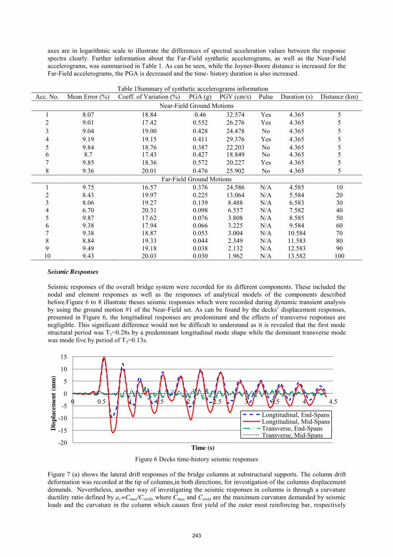
Seismic Responses Seismic responses of the overall bridge system were recorded for its different components. These included the nodal and element responses as well as the responses of analytical models of the components described before.Figure 6 to 8 illustrate theses seismic responses which were recorded during dynamic transient analysis by using the ground motion #1 of the Near-Field set. As can be found by the decks’ displacement responses, presented in Figure 6, the longitudinal responses are predominant and the effects of transverse responses are negligible. This significant difference would not be difficult to understand as it is revealed that the first mode structural period was T1=0.28s by a predominant longitudinal mode shape while the dominant transverse mode was mode five by period of T5=0.13s.

Figure 6 Decks time-history seismic responses

Figure 7 (a) shows the lateral drift responses of the bridge columns at substructural supports. The column drift deformation was recorded at the tip of columns,in both directions, for investigation of the columns displacement demands. Nevertheless, another way of investigating the seismic responses in columns is through a curvature ductility ratio defined by μc=Cmax/Cyield, where Cmax and Cyield are the maximum curvature demanded by seismic loads and the curvature in the column which causes first yield of the outer most reinforcing bar, respectively

-20

-15

-10

-5

0

5

10

15

0 0.5 1 1.5 2 2.5 3 3.5 4 4.5

Disp

lace

men

t (m

m)

Time (s)

Longtitudinal, End-Spans Longtitudinal, Mid-Spans Transverse, End-Spans Transverse, Mid-Spans

243

(Nielson 2005). Therefore, in addition to the columns drift, the columns’ seismic responses were recorded in terms of Moment-Curvatureat the columns’ base, as shown in Figure 7 (b).The seismic responses of the analytical models of the bridge components are shown in Figure 8. As it is understood, the portion of pile resistance in transverse direction is minor while it is quite significant in the longitudinal active direction.Comparing the seismic responses of the four elements presented in this figure with the decks’ deformation responses in Figure 6, it is evident that most of thedisplacement in longitudinal directionisdemanded by deformation in the abutment piles.This happened while the passive soil resistance still showed linear responses.The response of the impact element, presented in Figure 8 (b), indicates that the initial gap in impact elements (expansion gap between adjacent decks) was not closed under seismic loads. A similar trend is observed both in the fixed and expansion bearings’ responses, as illustrated by Figures 8 (a) and (b) as not many hysteric loops were recorded by these elements. This would be due to the large stiffness of elastomeric pads which have been assigned to the bearing elements.

Figure 7 Columns seismic responses: a) drift deformation and b) moment-curvature hysteretic loops

-3E-3

-2E-3

-1E-3

0E+0

1E-3

2E-3

3E-3

0 0.5 1 1.5 2 2.5 3 3.5 4 4.5

Col

umn

Dri

ft

Time (s)

Mid-Col_Long Mid-Col_Trans End-Col_Long End-Col_Trans -6E+5

-4E+5

-2E+5

0E+0

2E+5

4E+5

6E+5

-2E-6 -1E-6 0E+0 1E-6 2E-6

Mom

ent (

N.m

m)

Curvature (1/mm)

Mid-Col_Long Mid-Col_Trans End-Col_Long End-Col_Trans

(a) (b)

244

Figure 8 Nonlinear seismic responses of the analytical model: a) abutment, b) impact, c) fixed bearing and d) expansion bearing elements.

Probabilistic Seismic Demand Analysis Among the recorded seismic responses, the columns’curvature ductility (μc), longitudinal deformations in the fixed and expansion bearings, and active and passive deformations in the abutments were nominated as the seismic demand parameters for performance assessment of the bridge system, since they have been reported to be determinant in evaluating the seismic capacity of highway bridges (Nielson andDesRoches 2007). Figures 9 (a) to9 (e) show the developed IDA curves for these bridge components.

-2E+5

-1E+5

-5E+4

0E+0

5E+4

1E+5

2E+5

-10 0 10 20 30

Forc

e (N

)

Deformation (mm)

Longitudinal Transverse

-1

-0.8

-0.6

-0.4

-0.2

0

-6 -4 -2 0

Forc

e (N

)

Deformation (mm)

Impact Element

-2E+5

-2E+5

-1E+5

-5E+4

0E+0

5E+4

1E+5

-6 -4 -2 0 2

Forc

e (N

)

Deformation (mm)

Longitudinal Transverse

-2E+5

-1E+5

-5E+4

0E+0

5E+4

1E+5

2E+5

-2 0 2 4 6 8

Forc

e (N

)

Deformation (mm)

Longitudinal Transverse

(a) (b) (c)

245

Figure 9 Developed IDA forsignificant bridge components; a) column, b) fixed bearing, c) expansion bearing, d)

abutment in active direction and e) abutment in passive active direction

Except the fixed bearing, which demonstrates a severe hardening, the other components show a softening or a slight hardening behaviour. This happened while the deformations demanded in the fixed bearing were much smaller than the deformations demanded in the expansion bearings. The reason for this behaviour could be the large initial gap, due to expansion washers, assigned to the expansion bearings which permitted larger deformations while the absence of such a gap in the fixed bearings resulted in the yielding of steel dowels. As understood from Figure 9 (d), the abutment piles had the main contribution in the bridge’s deflections under seismic forces. This was mainly due to the quantities which were assigned to the element properties of different bridge components. As mention previously, the bridge analytical model developed for this study represented a generalised highway bridge. Therefore, this contribution may be different in other cases or other concrete

0

0.2

0.4

0.6

0.8

1

1.2

1.4

0 0.2 0.4 0.6 0.8 1 1.2

Spec

tral

Acc

eler

atio

n (g

)

Ductility Ratio (μc)

NF1

NF2

NF3

NF4

NF5

NF6

NF7

NF8

FF

0

0.2

0.4

0.6

0.8

1

1.2

1.4

0 2 4 6 8 10

Spec

tral

Acc

eler

atio

n (g

)

Deformation (mm)

0

0.2

0.4

0.6

0.8

1

1.2

1.4

0 10 20 30 40

Spec

tral

Acc

eler

atio

n (g

)

Deformation (mm)

0 0.2 0.4 0.6 0.8

1 1.2 1.4

0 20 40 60 80

Spec

tral

Acc

eler

atio

n (g

)

Deformation (mm)

0 0.2 0.4 0.6 0.8

1 1.2 1.4

0 2 4 6 8 10

Spec

tral

Acc

eler

atio

n (g

)

Deformation (mm)

(a)

(b) (c)

(d) (e)

246

bridges. In addition, for further investigation of the bridge seismic performance, a stripe analysis (Jalayer2003) was performed over the IDA column ductility responses, as shown in Figure 10.Then, the well-accepted power model distribution suggested by Cornel et al. (2002) was used to establish a relation between the spectral accelerations (analyses inputs) and the columns’ ductility (seismic demands). This was performed using the median seismic demand values of the Near-Field results and original Far-Field seismic responses.

Figure 10 Stripe analysis of the IDA analysis results by using the column ductility responses

The obtained equations, shown in Figure 10, can be used to predict the columnductility seismic responses of a highway bridge demanded by arbitrary shaking intensities. Note that these power models are valid for Near-Field and Far-Field earthquakes with maximum PGA of 0.9g and 0.48g, respectively. Using these equations, it is possible to evaluate the seismic performance of bridge components under different design earthquake levels. For example, taking the evaluated MCE for short-period structures in the city of Brisbane (SS=0.32g) into consideration, the demanded column ductility by the Near-Field and Far-Field seismic events are estimated as 27.72% and 34.54%, respectively. In addition, these power model distributions can be used to predict highway bridge column performancein various seismic hazard levels, as suggested by the probabilistic earthquake maps. Nevertheless, the most significant use of such distributions is in finding closed-form solutionsfor seismic fragility analysis of bridge components or an overall bridge system.This would provide an appropriate insightfor seismic vulnerability and risk assessment of Australian bridges through developing bridge fragility curves. Development of such curves for selected bridges would profit the bridge asset managers and stakeholders and the regulatory authorities in the adoption of state or national plans for mitigating future seismic hazards. This last pointis the ultimateobjective of performance-based earthquake and structural engineering. CONCLUSION A studyhas been presented herein for the seismic performance assessment of a MSSS concrete box-girder highway bridge by creating an analytical model in OpenSees software. A suit of synthetic ground motions was created, based on a GMP model, to properly simulate the circumstances of Australian earthquakes. It is noteworthy to mention that these strong ground motions will bevery beneficial for further seismic studies relevant to Australia.IDA analyses were also performed over the analytical model to investigate the bridge seismic responses. The probabilistic seismic performance of the bridge columns was obtained through a stripe analysis over the IDA responses and by fitting the well-accepted power model to the median values. This model can be used further to develop the seismic fragility curve of bridge columns. ACKNOWLEDGMENTS The authors gratefully acknowledge the support provided by Queensland Department of Transport and Main Roads (TMR).TMR, throughDr. Ross Pritchard,playedanimportantroleinprovidingthenecessary information. In addition,the authors would like to acknowledge the vital support of Dr. Bryant Nielson, Professor Paul Somerville and Associate Professor Jack Baker to this study.

0

0.2

0.4

0.6

0.8

1

0 0.2 0.4 0.6 0.8 1 1.2

Spec

tral

Acc

eler

atio

n (g

)

Column Ductility Ratio (μc)

Striped Values_Near-Field Median Values_Near-Field Far-Field Values

μc= 1.0073Sa1.1322Near

-Field

μc= 0.9807 Sa0.9159Far-Field

247

REFERENCES Baker, J.W., Cornell, C.A., (2006). “Which spectral acceleration are you using?”,Earthquake Spectra, 22 (2),

293-312. Choi, E. (2002). “Seismic Analysis and Retrofit of Mid-America Bridges”, PhD Thesis, Georgia Institute of

Technology, GA, USA. Cornell, C.A., Jalayer, F., Hamburger, R.O. and Foutch, D.A. (2002).“Probabilistic Basis for 2000 Sac Federal

Emergency Management Agency Steel Moment Frame Guidelines”,Journal of Structural Engineering, 128(4), 526-533.

Cornell, C.A. and Krawinkler, H. (2000). “Progress and Challenges in Seismic Performance Assessment”, PEER Center News, pp. 1-3.

Geoscience Australia.(n.d.). “Historic Events - Earthquakes”, Retrieved from http://www.ga.gov.au/scientific-topics/hazards/earthquake/basics/historic

Jalayer, F. (2003). “Direct Probabilistic Seismic Analysis: Implementing Non-Linear Dynamic Assessments”,PhD Thesis, Stanford University, CA, USA.

Leonard, M., Burbidge, D. and Edwards, M. (2013). “Atlas of seismic hazard maps of Australia: seismic hazard maps, hazard curves and hazard spectra”, Record 2013/41. Geoscience Australia: Canberra.

McKenna, F. and Feneves, G. L. (2005). “Open System for Earthquake Engineering Simulation”, Pacific Earthquake Engineering Research Centre, Version 1.6.2.

Muthukumar, S., and DesRoches, R. (2006).“A Hertz Contact Model with Non-linear Damping for Pounding Simulation.”Earthquake Engineering and Structural Dynamics, 35(7), 811-828.

Nielson, B. G. (2005). “Analytical Fragility Curves for Highway Bridges in Moderate Seismic Zones”, PhD Thesis, Georgia Institute of Technology, GA, USA.

Nielson, B. G. and DesRoches, R. (2007), “Seismic fragility methodology for highway bridges using a component level approach”, Earthquake Engineering & Structural Dynamics, 36(6) 823–839.

Queensland Department of Main Roads, Road System and Engineering., (2004). “BridgeInspectionManual” (Registration Number 80.640).Brisbane, Australia.

Seismic Design Maps & Tools: Worldwide Seismic Design Tool (Beta), (2011)., Retrieved from http://geohazards.usgs.gov/designmaps/ww/

Seismosoft: Eathquake Engineering Software Solutions, (2002). , Retrieved from http://www.seismosoft.com/ Somerville P., Graves R., Collins N., Song S.G. and Ni S., (2009). “Source and Ground Motion Models for

Australian Earthquakes”, Geoscience Australia: Canberra. Vamvatsikos, D. and Cornell, C. A., (2002), “Incremental dynamic analysis”, Earthquake Engineering &

Structural Dynamics, 31(3) 491–514.

248